Thermal stratification in raw sewage stabilization ponds

Item Type text; Thesis-Reproduction (electronic)

Authors Pisano, William C.

Publisher The University of Arizona.

Rights Copyright © is held by the author. Digital access to this materialis made possible by the University Libraries, University of Arizona.Further transmission, reproduction or presentation (such aspublic display or performance) of protected items is prohibitedexcept with permission of the author.

Download date 24/05/2018 15:25:45

Link to Item http://hdl.handle.net/10150/319693

THERMAL STRATIFICATION IN RAW SEWAGE STABILIZATION PONDS

byWilliam Chauncey Pisano

A Thesis Submitted to the Faculty of theDEPARTMENT OF CIVIL ENGINEERING

In Partial Fulfillment of the Requirements For the Degree ofMASTER OF SCIENCE

In the Graduate CollegeTHE UNIVERSITY OF ARIZONA

1964

STATEMENT BY AUTHOR

This thesis has been submitted in partial ful­fillment of requirements for an advanced degree at The University of Arizona and is deposited in the University Library to be made available to borrowers under rules of the Library.

Brief quotations from this thesis are allowable without special^ permission, provided that accurate acknowledgment *bf source is made. Requests for permis­sion- for- extended quotation from or reproduction of this manuscript in whole or in part may be granted by the head of the major department or the Dean of the Graduate College when in his judgment the proposed use of the material is in the interests of scholarship. In all other instances, however, permission must be obtain­ed from the author.

SIGNED: [ iL f j L w v i

APPROVAL BY THESIS DIRECTOR This thesis has been approved on the date shown below:

Quentin M. Mees Professor of Civil Engineering

ACKNOWLEDGEMENTS

The author is deeply indebted to Quentin M . Mees, "Professor d'f Civil Engineering, for his encouragement and assistance in the preparation of this thesis. To Doctors Emmet M . Laursen and Simon Ince an expression of apprecia­tion is also given for their suggestions.

Gratitude is extended to Pima County Sanitary Dis­trict No. 1 for making available the facilities at which the study was conducted. To the Department of Civil Engineering the author expresses his appreciation for their cooperation in making available the necessary laboratory facilities.

Appreciation is also extended to two fellow colleagues, Clinton E . Parker and Robert B. Conklin II, for their ideas and physical assistance. A lasting debt of thanks is extend­ed ;to Lynn Wilcox who faithfully gave up his time to man the oars .

ill

TABLE OF CONTENTS

PageINTRODUCTION. . . . . . . . . . . . . . . . . . . . . 1

l.T General Discussion . . . . . . . . . . . . . 11.2 Stabilization Pond Characteristics . . .... . 21.3 Purpose' and Scope of Thesis. . . . . . . . . 3,1.4 Location of Stabilization Pond . . . . . . . 51.5 Description of Installation. . . . . . . . . 5

CONCEPTS -AND DEFINITIONS. ' . . . . . 8

2.1 Detention Time . . . . . . . . . . . . . . . 82.2 Specific Weight. . . . . . . . . .......... 82.3 Causes of Stratification . . . . . . . . . . 92.4 Seasonal Change in Thermal Stratification. . 132.5 Influent and Effluent Considerations . . . . 152.6 Wind Effects . . . . . . . . . . . 172.7 Thermal Effect of Mixing . . . . . . . . . . 212.8 Stability of Stratification. ........... 222.9 Air Diffusion. ............... 232 .10 Coliform Bacteria. . . . . . . . . . . . . . 25

PREVIOUS INVESTIFATIONS . ............ .(. .............. 283.1 Short-Circuiting in Stabilization Ponds. . . 28. . 3.1.1 Previous Pond Study . . . . . . . . . 293.2 Retention of Pathogens . . . . . ......... 333.3 Wind Effects . . . . . . . . . . . . . . . . 343.4 Detection of Short-Circuiting Using

Coliform Bacteria. . . . . . . . . . . . 353.5 Air Diffusion Considerations . . . . . . . . 37

3.5.1 Applications of Air Diffusors . . . . 393.5.1.1 Pneumatic Breakwaters. . . . 393.5.1.2 Prevention of Salt-Water

Intrusion. . . . . ... .• 393.5.1.3 Ice Prevention . . . . . . . 403.5.1.4 Aeration of Oxidation Ponds. 40

3.5.2 Design Criteria for a DiffusionSystem. . . . . . . . . ........ 42

METHODOLOGY . . . . . . . . . . . . . . . . . . . . . 434.1 Selection of Coliform Sampling Equipment . . 43

4.1.1 Description of ABC Sampler andVac Ampules . . . . . . . . . . . 43

iv

VTABLE OF CONTENTS— Continued •

•Page4.1.1.1 Operation of. Sampler. . . . 44

4.1.2 Selection of Identifying Technique . . 444.1.2.1 Description of Millipore

Filter Technique. . . . . 444.1.2.2 General Notes on Procedure. . 46 ■

4.2 Temperature Measuring Equipment .......... 474.2.1 Thermistor - Bridge Assembly . 474.2.2 Other Temperature Measuring

Equipment. . . . . . . . . . . . . . 514.3 Selection of a Tracer Study Procedure . . . . 51

4.3.1 Instrumentation. 53.4.3.2 Selection of a Tracer Dye. . . . . . . 53

4.3.2.1 Temperature Varience ofElio dam ine B . . . . . . . 54

4.3.2.2 Method of Application . . . . 554.3 .2 .3 Density Effects of Dye

Solutions. ................ 574.3.3 Location of Sampling Platforms . . . . 58

4 .3 .'3.1 Construction of SamplingPlatforms . . . . . . . . 58

4.3 .3.2 Sampling Technique. . . . . . 604.4 Aeration Equipment......... 60

4.4.1 Tubing . • ..624.4.2 Alignment of Holes .................. 624.4.3 Placement of Tubing. . . . . . . . . . 624.4.4 Mechanical Equipment ............ 64

PRESENTATION OF DATA . . . . . . . . . . . . . . . . 6 6

5.1 Coliform Bacteria1 Studies . . . . . . . . . . 6 65.1.1 Observations, August 1, 1963 . . . . . 6 65.1.2 Observations", August 2, 1963 . .. . . , 6 65.1.3 Observations, November 1, 1963 . . . . 69

5.2 Temperature Measurements. . . . . . . . . . . 695.2.1 Measurements, October 3, 1963..... 745.2.2 Measurements, October 5, 1963. . . . . 745.2.3 Measurements, November 1, 1963 . . . . 765.2.4 Influent Area Study, February 20,

19 C5 4 ° . . . e o o e . . . . , a . 7 55.2.5 .Influent Area Study, March 12, 1964. .. 76

5.3 Tracer Studies. . . . . . . . . . . . . . . . SO5.3.1 Tracer Study, October 5, 1963. . . . . 815.3.2 Tracer Study, November 20, 1963. . . . 84 .5.3.3 Effluent Study, November 20, .1963. . . 84

• viTABLE OF CONTENTS— -Continued

Page5.3.4 -Aeration-Tracer Study, November 22,

1 9 6 3 . . . . . . . . . . . . . . . 875.3.5 Aeration-Tracer Study on February 21,

1964e e o e e e e e e o e . e e . 94DISCUSSION OF RESULTS . . . . . . . . . . . . . . . . 100

6.1 Coliform Bacteria. . . . . . ... . . . . . . . 1006.1.1 Coliform Density in Effluent

Study, August 1, 1963 . . . . . . 1006.1.2 Vertical Coliform Density Profiles,

August 9, 1963. . . . . . . . . . 1016.1.3 Coliform Study, November 1, 1963. . . 102

6.2 Temperature Measurements . . . . . . . . . . 1026.2.1 Temperature Measurements, October 3,

1963. . . . . . . . . . . . . . . 1026.2.2 Influent Area Measurements. . . . . . 103

6.3 Tracer Studies . 1036.3.1 Tracer Study, October 5, 1963 . . . . 1036.3.2 Tracer Study, November X, 1963. , . . 1046.3.3 Effluent Study, November 20, 1963 . . 105

6.4 Aeration-Tracer Studies. . . . . . . . . . . 1056.4.1 Aeration-Tracer Study, November 22,

1963. ........ 1056.4.2 Aeration-Tracer Study, February 21,

1964 .......... 107CONCLUSIONS & RECOMMENDATIONS . . . . . . . . . . . . 110

7.1 General Conclusions. . . . . . . . . . . . . 1107.2 Recommendations. . . . . . . . . . . . . . . Ill7.3 Suggestions for Future Study . . . . . . . . 112

APPENDIX. . . . . . . . . . . . . . . . . . . . . . . . 114

LIST OF ILLUSTRATIONS

Figure Page1.1 Schematic Diagram of Stabilization Lagoon

Process I . . . . . . . . . . . . . . . . . . . . 41.2 ■ Stabilization Lagoon. Site. . . . . . . . . . . . 6

2.1 Change in Specific Weight with Temperatureand Salinity . . . . . . . . . . . . . . . . 10

2.2 Effect of Solar Radiation and Wind Action onTemperature - Depth Relationship . . . . . . 11

2.3 . Seasonal Variations of Temperature Gradients . . 142.4 Climatogical Data, Tucson, Arizona, 1962-f 1^63 . . 162.5 Possible Paths of Influent Movement, . . . . . . 182.6 Wind Effects 202.7 Diagram for Calculating Stability. . . . . . . . 242.8 Qualitative Pattern of Surface Currents

Produced by Air Bubbles. . . . . . . . . . . 263.1 Average Hourly DO, pH, and Temperature Values

6/11/62 - 7/30/62. . . . . . . . . . . . . 303.2 Flow Patterns, August 10, 1962 Tracer Study. . . 323.3 Typical Hinde Installation .......... 414.1 . ABC Sampler (left) and Millipore Filter

Apparatus .............. 454.2 Wiring Diagram of Temperature Measuring

Apparatus.......... 484.3 Calibration Curve for Thermister-Bridge

Assembly . . . . . . . . . . 504.4 Temperature Measuring Equipment. Foxboro

Portable Indicator (right) . . . . . . . . . 52

v i i

viiiLIST OF ILLUSTRATIONS--Continued

Figure Page4.5 Fluorometer Calibration Curves. . . . . .. . . . 564.6 Sampling Platforms .........- ............. . 594.7 Diffusion Piping Arrangements . . . . . . . . . 614.8 Alignment Rod Attachment. « '. '.V . .' . . . . . 634.9 Compressor and Instrumentation. . . . . . . . . 655.1 Coliform, Ambient and Surface Temperatures

vs. Time at the Effluent Structure. . . . . 675.2 Coliform Profile, Station 3, 1030,

August 9, 1963 705.3 Coliform Profile, Station 9, 1030

August 9, 1963. . . . . . . . . . . . . . . 715.4 Coliform Profile, Station 9, 1600

Aug. 9, 1963. . . . . . . . . . . . . . . . 725.5 Coliform Profile, Er, 1330, Nov. 1, 1963. . . . 735.6 Temperature Measurements, Oct. 3, 1963. . . . . 755.7 Temperature Profile, Station 3, Oct. 5, 1963. . 775.8 Temperature Measurements, Nov. 1, 1963. . . . . 785.9 Temperature Measurements in the 'influent

Area, February 20, 1964 . . . . . . . . . . 795.10 Temperature Measurements in the Influent

Area, March 12, 1964. . . . . . . . . . . 815.11 Visible Dye Movements, Oct. 5, 1963 . . . . . . 825.12 Dye Profiles at Sampling Platforms - E4

and Effluent, Oct. 5, 1963. . . . . . . . . 835.13 Visible Dye Movements, Nov. 1, 1963 . . . . . . 855.14 Dye Profiles at Sampling Platform E%,

Nov. 1, 1963. . . . . . . . . . . . . . . . 8 6

LIST OF ILLUSTRATIONS— Continuedix

Figure ' Page5.15 Visible Dye Movement, Nov. 20, 1963. . . . . . . 8 85.16 Tracer Study, Nov. 20, 1963. . . . . . . . . . . 895.17 Visual Dye Movements. Aeration-Tracer Study,

Nov. 23, 1963. . . . . . . . . . . . . . . . 915.18 Dye Movements, Aeration-Tracer Study,

Nov. 23, 1963. . . . . . . . . . . . . . . . 925.19 Dye Movements, Aeration-Tracer Study,

' Nov. 23, 1963 . . . . . . . . . . . . . . . . 935.20 Tracer Dye Profiles at Sampling Platforms

Ei - E4 and Effluent, Oct. 5, 1963 . . . . . 955.21 Dye Movements, Aeration-Tracer Study

Feb. 21, 1 9 6 4 . . . . . . . . . . . . . . . . 965.22 Subsurface Dye Movements, Aeration-Tracer

Study, Feb. 21, 1964 . . . . . . . . . . . . 975.23 Tracer Dye Profiles at Sampling Platforms

Ef - E4 and Effluent, Feb. 21, 1964. . . . . 99

ABSTRACT

A raw sewage stabilization pond located near Tucson, Arizona, owned and operated by the Pima County Sanitary District No. 1 was.used during a seven month study to deter­mine whether or not thermal stratification would appreciably effect detention time.

Since time is required for oxidation of putrescible wastes and for elimination of water-borne pathogens that may enter the basin, detention time is one of the more important process controls. It is known that Entamoeba histolytica, causative agent of amebic dysentery, can.remain viable in sewage, for at least six days and therefore must be retained a longer period of time to insure complete elimination.

Using temperature profiles, bacterial distributions, and velocity profiles, flow-through times of 2 to 6 hours were found to exist during the autumn and winter seasons.

Mixing by air diffusion was investigated using velocity profiles as the basis for evaluation. Two geometric configurations of perforated plastic tubing were used to create relatively small mixing cells. Aeration rates of 0.05 and 0.25'cubic feet per minute per foot of aeration tubing were found to be unsatisfactory for mixing the stratified flow. '

x

Chapter 1

INTRODUCTION

101 General DiscussionIt was once said by G* Mo Fair (1) that a sewage

treatment plant is like a river wound up into a very small place. All.the biophysical.factors which act on putrescible wastes in a stream are also at work in conventional sewage treatment. Stabilization lagoons, which epitomize rivers, are becoming more widely used in lieu of the conventional units and provide the same purifying processes for far less cost. This is especially true in the Southwest where land costs are low.

In general, the effectiveness of these ponds is controlled by parameters such as the imposed biological loading, the detention time, the amount of sunlight, the temperature of the ambient atmosphere, and a host of others. It is generally agreed that a hot sunny climate is most conducive to optimum stabilization of wastes. However, this may not be entirely true, Temperature stratification, re­sulting from extreme ambient temperatures, may be most unde­sirable . Severe short-circuiting caused by temperature- V induced density currents may drastically limit the success of a pond.. . ..

- ' .2 Although exceptions exist, experience has shown

that stabilization ponds can produce a well-treated effluent. Effluents are. generally odorless, low in biological oxygen demand, and reductions in bacteria are for the most part very high. They are generally high in fertilizer value and may be benefically used in the irrigation of non-edible crops. Effluents have been used for construction purposes and for the development of recreation areas (2). Simple disposal into streams and lakes is common.

Whatever the use or method of disposal, some of the effluent will be eventually, re-used by people. In the South­west where existing water supplies are being rapidly depleted, direct recycle of waste-water takes' on :a more significant aspect. Since the stabilization pond is.a complete treatment plant wound up in one confined body of water, any change in a major parameter may change the entire picture.

1.2 Stabilization Pond CharacteristicsThe Arizona State Health- -Department has set the

following requirements for stabilization ponds; 1 ) total ■detention tAme, should be at least 2 0 days; 2 ) imposed bio­logical loading should not exceed 50 pounds per acre of surface area per day; 3) depths should be 3 to 5 feet; and 4 ) inlets should be center-placed.

Stabilization of putrescible organic wastes is accomplished by aerobic and anaerobic decomposition. The

stabilization process is schematically illustrated by Figure 1.1. Oxygen in the aerobic reach is supplied by the photosynthesis of algae and by atmospheric mixing. This algal-laden upper zone, rich in dissolved oxygen content, rapidly decomposes wastes and oxidizes odorous gases. The bottom benthal zone is generally characterized by a deficit in oxygen'. In this layer the slower and less complete anaerobic decomposition takes place. Vast quantities of ammonia, carbon dioxide, methane, and products of incomplete oxidation are released from these deposits.

1.3. Purpose and Sbope of ThesisTo render a waste chemically stable and free of

dangerous organisms at the lowest possible cost is good sanitation practice. To assess the true worth of any unit, all of its capabilities must be known to the fullest extent possible. Evaluation of operational parameters is of special public health significance when direct reuse of the waste is not remote.

Since time is required for ecosystems to develop, to assimilate food, and to finally reduce each other, deten­tion time in a stabilization pond is one of the more impor­tant process controls. A study of this .parameter on a prototype scale would be of fundamental interest to both the medical and engineering professions. It was with this ob­jective in mind that a study of the effect of thermal

Wind Sun

Lagoon Surface

CO AerobicAlgae

Raw SewageBacteria(settleable

solids)

AnaerobicBcnthal Deposits

Bacteria

FIGURE 1.1.Schematic Diagram of

Stabilization Lagoon Process

5stratification on detention time was initiated. Parameters to be evaluated included temperature profiles, bacterial distributions, and velocity profiles. In addition, air diffusion as a mixing-agent was to be investigated using velocity profiles as the basis for evaluation.

1.4. Location of Stabilization PondThe basin studied in this thesis is located six

miles Northwest of the city limits of Tucson, Arizona, pond is owned and operated by the Sanitary District No. of Pima County, Arizona, which uses stabilization ponds treat waste-water that cannot be treated by the City of Tucson's sewage.treatment plant.

1.5. Description of InstallationTwo ponds are operated in series with an inflow of

about 300,000 gallons per day of domestic sewage. They have a combined surface area of 3.8 acres, average about 5 feet in depth, and are rectangular in shape. Figure 1,2 shows the general arrangement. In this study all investigations were conducted on the primary pond.

The inlet to the primary pond is located 30 feet south of the top of the north bank and 60 feet west of the centerline of the east dike. . Another inlet symmetric to the first on the west side of the pond was plugged throughout the entire project. The outlet of the primary pond is a surface overflow pipe located at the southeast corner.

The1

to

PrimaryO

Station 3

OStation 6

o o o o;A ° Ei4 station 9 1

Effluent

Secondary

j

4-

Flume Manhole

A

N

Dike Slope Depth o*

Primary Area 2.0 Acres Secondary Area 1.8 Acres

FIGURE 1.2 STABILIZATION LAGOON SITE

Stations 3, 6 , and 9, shown on Figure 1.2, are steel pipes driven into the bottom of the basin and were used in this project as sampling locations. They are located at the centerline third points in the pond. Sam­pling platforms through are also shown. See section4.3.3 for their location and application.

Chapter 2

CONCEPTS AND DEFINITIONS

2.1. Detention TimeFor purposes of this study the definition of

detention time has been qualified. It.is defined as the time required for the first unit volume of fluid/to pass through the ..basin, under consideration .

Many factors influence this parameter. The proper­ties of the fluid which passes through the basin, atmos­pheric conditions, geometry of the basin, and inlet and outlet configurations are but some of these factors. Perhaps most significant and most basic of these influences are the fluid properties and wind movement.

■2.2. Specific WeightThe specific weight of a fluid is the weight con­

tained in a unit volume. Water is a unique fluid in that the density reaches a maximum at 40C and becomes lighter asthe temperature either decreases to 0°C or increases beyond o4 C . As the temperature increases the decrease in specific weight per unit degree change becomes larger. Dissolved and suspended solids also influence the specific weight. However, these changes are generally small in comparison' with thermal changes for most waters. ..

- 8 - . ' ' "

9Figure 2.1 illustrates that at lower temperatures

anomalies can easily occur with small changes is salinity. However, as the temperature rises, salinity effects become secondary, that is, the weight change from 20°C to 25°C is 5 times the change due to a salinity increase or decrease of 2 0 0 mg/1 .

2.3. . Causes of StratificationWhen the temperature of a body of water changes with

depth, neglecting salinity changes, this body is said to be thermally stratified. Excluding inflow at varying tempera­tures, solar radiation, air-water surface conductance, terrestrial heat, and condensation are the possible sources' of heat for a lake. The most significant of these for most waters is solar radiation.

A portion of solar radiation reaching the earth’s .surface will be partially reflected upward and # portion will be absorbed by the uppermost layers of a lake. The heat-producing infrared and longer wavelenghts will be rapidly attenuated and converted to heat. Portions of the shorter wavelenghts, that is, the blue,blue-green, etc, will also be absorbed depending upon the dissolved solid content (this factor generally determines the color of the water). This phenomena is illustrated by curve A in Figure 2 .2 .

Change

in Specific Weight #/ft.

Salinity mg/110

0 200 400 600 800 1000

co

.25

.20

15Temperature

10

Salinity05

10 15 20Temperature °C FIGURE 2.1

25 30

Change in Specific Weight with Temperature and Salinity

BA. Solar Radiation only

A B. Effect of Wind on A.

TEMPERATURE

FIGURE 2.2Effect of Solar Radiation and Wind Action

On Tempcrature-Depth Relationship (1.)

■ : . -12 Heat absorbed by the surface is distributed into the

lower reaches by the mixing action of the wind. Whenever a wind blows over a lake, it exerts a shearing stress at the ■ air-water interface, in consequence of which the water is accelerated. This movement of water will result in the piling of water in one- part of the basin and a lowering of the surface in another part. The slope so developed will cause a gradient current to start flowing, and the system will come to equilibrium when the transport due to the wind is balanced by a return transport due to the gradient cur­rent (3). Currents may travel at or below the surface depending upon the topography of the shore line and the orientation of the wind fetch. Turbulence and corresponding vertical and horizontal intermixing of heat gradually deepens the warm layers. Extent of mixing will depend upon the mag­nitude of the wind and the temperature change with depth. Curve B in.Figure 2,2 shows this effect.

The upper circulating zone is called - the epilimnion. Temperatures are relatively higher and variations are slight in this zone. The region of rapid temperature decrease or transition is classified as the thermocline« In the lower portion of a lake, a quiescent body termed the hypolimnion exists .

132.4. Seasonal Change in Thermal Stratification

Interplay of temperature, density, and wind during the different seasons of the year produce a characteristic pattern for thermal stratification of lakes. Figure 2.3 shows a series of characteristic gradients for waters in the middle latitudes of the temperate zone.

During the winter water just below a frozen lake is at 0°C with a bottom temperature around 4°C, the temperature of maximum density. The water is in comparatively stable equilibrium and is inversely stratified (thermally).

As the ice breaks up in the spring, water at the surface warms up and sinks. Instability caused by diurnal flucuations in temperature and aided by wind results in vertical circulation. This becomes more pronounced when the temperature of the water throughout the vertical is practically uniform and close to the temperature of maximum density. This is the condition of spring circulation.

During the summer the surface water becomes progres­sively warmer. Lighter water overlies denser water, and, as the temperature differences increase, circulation is confined more and more to the upper layers. A second period of stable equilibrium is established and the water becomes directly stratified. '

With the coming of autumn convective currents are set up as the surface cools and sinks. Instability takes

Winter

Stagnation

14

• H+->

TEMPERATURE

FIGURE 2.3Seasonal Variations of Temperature Gradients

' , 15place once again, The region which was previously warm slowly sinks into the depths. When the temperature gradient becomes vertical the entire basin is easily put into circu­lation. With a drop in surface temperature to 0°G,and a quiescent period, the lake will freeze.

The above description would have to be modified for a shallow lake located at a relatively low altitude which endures a high diurnal temperature change as would be found in the Tucson basin. With some qualifications, the seasonal variations indicated in Figure 2.3 may take place in the course of a day. Water rarely freezes in the winter and would probably reach a minimum of 6°C. Extreme daily ambient temperature flucuation experienced by the Tucson Valley are " illustrated in Figure 2.4. Warm days during the winter are not the exception. Sharp stratification may occur on a hot quiescent day in December with the corresponding partial overturn during the night. During the summer months the ambient diurnal temperature change may produce a well defined themocline during .the day while cooling at night causes severe overturn due to the shallowness of the lake and the vast density change in the higher temperature range.

2.5. Influent and Effluent ConsiderationsThe path of a parcel of water entering a basin is

dependent upon its density and the density of the fluid in the basin. In general, four paths of movement are possible:

Possible

Sunshine

Percent

Temp

erat

ure

16

120

Maximum100

40

M inimuin20

July Aug. Oct.Sept. Nov. Dec . AprilMarchFeb JuneMayJan .

1962 19G3

100 T7T80

60

20

July Sept. Oct.Aug. Nov. Dec AprilMarch JuneFeb MayJanFIGURE 2 .4

Climatogical Data Tucson, Arizona

1962-1963

171) if its density is lighter than that of the entire basin, it will float and move over the surface; 2) if its density can be matched, flow will occur in the region of greatesttemperature-density gradient the thermocline; 3) if itsdensity is greater than any layer, underflow will occur;4) if its density is the same at every level in the pond, a uniform movement will take place. Figure 2.3 shows the possibilities where inflow occurs near the bottom. In view of the above statements, vertical placement of the effluent pipe is of prime importance in retaining the fluid as long as possible. Draw-off should be at the bottom for the first two cases, at the top for the third, and anywhere for the fourth. The basin in this study had a surface overflow pipe .

2.6. Wind EffectsIt has been mentioned that wind is the prime factor

which distributes heat throughout the depths in a lake. Mixing the volume of the influent with the contents of thetpond also results. Oxygen replenishment through continual interfacial exchange is another benefit of wind movement. However, wind may have some adverse effects. Gradientcurrents may be accentuated to some extent. The time requir­ed to throughly mix the contents of the influent with thatof the pond and the rate of surface movement may not be thes ame.

Depth

Surface Flow Thermocline Flow

Under Flow Uniform Flow

Dashed line representsthe temperature profile

FIGURE 2.5 Possible Paths of Influent Movement

19In the previous section mention; was made of the

four possible paths of movement. Figure 2.6 shows how the wind can influence these movements.

In the first case, if the wind is in the directionof flow the gradient current will be accentuated (A). Sur­face draw-off aggravates the situation. If the wind opposes the direction of flow, either an undercurrent (B) or surface current in the direction of flow (C) will occur depending upon the orientation of the wind fetch and duration of wind.

When the incoming flow passes through the thermo- cline, as in the second case, wind opposing the direction of flow will hasten its movement (D^). The opposite is true for wind in the direction of flow (Dg)•

Underflow movement itself will generate a secondary circulation in the upper layers of the basin (E). The effect of wind on evaporative cooling may influence the convective displacement of the lower fluids upwards. This would also be true of the second case.

In the fourth case the currents generated by thewind can pass unhindered to all depths and the contents of the pond will be in continual motion (F). Rapid mixing of the influent with the entire contents of the pond may be undesirable in that portions of the flow undergoing treat­ment will immediately leave the pond.

(A) Wind in direction of surface movement

(C) Wind at a skew to basin for surface flow

(E) Underflow

(B) Wind opposes surface movement

(1)

(D) Wind with (1) against thermocline movement

Uniformly mixed

FIGURE 2-6Wind Effects

21It is interesting to note that the fourth case, with

or without wind, is generally the assumed condition for de­sign purposes. Where stabilization ponds are concerned, no consideration is ever given to the path of movement an in­fluent may take in a naturally stratified fluid.

It should be noted at this point that if density differences are caused by temperature only, salinity being constant, distinction between a warm buoyant unit volume of fluid just entering the basin and a detained volume experienc­ing the effects of solar radiation and wind action would be extremely difficult.

2.7. Thermal Effect of MixingMixing a column of water whose density varies with

depth such that it will become one of uniform density requires that physical work be exerted. Wind movement, mechanical paddles, and air diffusers are some of the sources that could supply this energy. The work required to mix a layer of water with another depends on the density difference between the two. It has been shown that temperature can signifi­cantly influence the density. Consequently, different amounts of energy must be expended to deliver heat into the depths. Birge (3) compares the work that must be supplied by the wind (or by any mechanical agent) in mixing layers of different temperatures by use of the' thermal resistance unit. A thermal resistance unit is defined as the ratio of

2 2

the work required to mix a cubic meter of water with a temperature gradient of 1°C to the work required to mix a 1°C difference at 4°C. Quantitatively expressed,

Thermal Resistance Unit <*=Density - Density

upper level lower level0,00008

Birge’s formula may be modified- to compare any temperature -density difference to any specified base con­ditions , Referring to Figure 2.1, the work required to mix a 5°C differential at 25°C would be approximately twice that required at 12°C. A sharp thermocline existing in warm waters may result in a considerable increase in the resistance to mixing.

The action of wind generates turbulence which in turn propagates heat, material, and momentum exchange. Material exchange or mixing the contents of a reactant within a reaction basin is of paramount importance if the desired reactions are to be attained,

2.8. Stability of Stratification.Schmidt (4) determined the expenditure of energy

necessary to upset an existing stratification or to bring it to a state where the whole water mass would have taken on the mean temperature by mixing. Considering a situation where a thermocline occurred, the center of gravity of this

23stratified body of water would be lower than if no strati­fication existed. Stability would be defined as the work required to raise the center of gravity an amount corres­ponding to its displacement downward from its original position. This is equivalent to lifting the weight of the basin a distance equal to the difference between the two centers of gravity.

Assuming that a basin had perpendicular walls and that an abrupt change in temperature existed between two layers of uniform temperature, stability would be expressed as:

S - (D2 - D^) (2h - z) z/2

Refer to Figure 2.7 for definition of terms.If 300,000 gallons per day of water at 2u°C flowed

into a basin of water 000 feet long and 180 feet wide at a temperature of 20°C, then 8,000 foot-pounds per day would have to be expended over the entire basin by some means to insure the elimination of a temperature-density varia­tion. Wind, convective cooling, and/or some other mixing device would have to supply this energy.

2.9. Air DiffusionAir diffusion provides a means of mixing stratified

flow. This mixing of the thermal strata would theoretically increase detention time.

I2r _ _ J

(A)

Stratification Mixed

(B)

4z/2

D. D

t - temperature D - Densityh - Depth to center of gravity of (B)” Center of gravity

z - Depth at which temperature changes

FIGURE 2.7 Diagram for Calculating Stability

25Releasing compressed air near the bottom of a body

of water defines the term "air diffusion"„ As air bubbles rise they impart a drag to the adjacent water particles resulting in an upward motion of an air-water mixture.When this: mixture reaches the surface, the air escapes, while the flow of water branches into two horizontal cur:-,..,. rents. Figure 2.8 indicates the qualitative flow patterns induced by the bubbling system.

2.10. Coliform BacteriaThe complete treatment of sewage encompasses both

the reduction of nuisance-causing putrescible wastes and the destruction of pathogenic organisms.

Knowledge of the rate of reduction of possible pathogens is desirable in the evaluation of a treatment pro­cess. With a stabilization pond, this takes on a deeper significance because of the absence of secondary units. Possibility of escape because of the result of stratifica­tion is not remote. Direct detection of disease-causing bacteria, protozoans, and viruses is most difficult and at times impossible. This is due to the extremely low density at which they occur, the complex laboratory techniques which must be employed, and the time required for positive identi­fication of these organisms. Fortunately, an indirect and-

VerticalVelocity

ProfileCurrent Velocity Profile

Streamline

AirSource

FIGURE 2.8Qualitative Pattern of Surface

Currents Produced by Air Bubbles

27simple means of indicating the possible presence of these pathogens is available. The Coliform bacteria group is used as an indicator.

The Coliform group is common to the, digestive - tract, is found in extremely large numbers in human feces, and is relatively easy to detect by routine procedures, This group is defined as aerobic and facultative anaerobic gram-negative nonspore-forming bacilli which ferment lactose with gas pro­duction within 48 hours at 35°C'(6). Two methods used in the enumeration of these organisms are the Most Probable Number (MPN) fermentation tube technique and the Membrane Filter(MF) differentiation media method. ’

8 10Human feces normally contain 10 to 10 coliform bacteria per gram. Domestic sewage contains, on the average, 0.5 million organisms per milliliter. Nearly all feces con­tain coliform organisms while only relatively small portion (2-20%) contribute pathogenic organisms (7). Thus domestic sewage could contain approximately 10,000 times as many coliforms as viruses. Enteric viruses, are the causative agents of infectious hepatitis, meningitisand poliomyelitis.

Coliform and virus populations in sewage are both subject to destruction due to the physical and biological forces which are employed in the treatment of sewage. Con­sequently, measuring.the reduction of coliform bacteria in a unit process will give some indication of the fate suffered by pathogens if they were present.

Chapter 3

PREVIOUS INVESTIGATIONS

3.1. Short-circuiting in Stabilization PondsA review of the literature revealed that very few

tracer studies have been conducted on stabilization ponds. Perhaps reflection on the lack of interest in this area might be summed up by a statement made by E. F . Gloyna (8) on this problem, "Due to the existence of long detention periods and corresponding low flow-through velocities . (in comparison with sedimentation velocities), short-circuiting is no p r o b l e m H i s statement is true if stabilization ponds are to function solely as sedimentation basins follow­ed by supplementary treatment. However, a stabilization pond is a complete treatment process. Elimination of patho­gens must be considered as one of . the primary functions of this process.

E. C . Trivoglou (9) conducted a tracer study on a partially frozen oxidation pond in South Dakota using radio­active isotopes . He found, as might have - been expected, that the warm sewage flowed in a stratified layer just be­neath the surface of the ice.

Merz, Merrell, and -Stone (10) conducted tracer studies on a pond in the Mohave Desert in 1957. The pond

—28 —

29was nine feet deep and exhibited stratification expected in a region with a hot ambient atmosphere. Using a fluorescein dye solution whose temperature matched that of the influent and no detection instrumentation, it was concluded that the inflow was mixed with the contents of the pond when the dye was no longer visible. Studies were conducted in both the presence and absence of wind movement. In all cases the dye disappeared in the immediate influent area of the basin.

3.1.1. Previous Pond StudySince 1960, Professor Quentin M. Mees and the Sani­

tary Engineering staff at the University of Arizona have conducted extensive operational studies on the oxidation pond used in this investigation. Contents of this- section were abstracted from a report entitled, ”Survival of Patho­gens in Sewage Stabilization Ponds’1. (11).

Figure 3.1 presents the average composite hourly values for temperature, dissolved oxygen, and pH recorded for top. and bottom samples accumulated at Stations 3 j 6, and 9 during seven sampling periods of 24 hours each. Average temperature of the raw sewage flowing into the pond is also presented. It should be significant to note that the temper­ature differential of the pond reached a maximum value of 4.5 C during the afternoon hours while the average influent temperatures were lower than the surface temperatures.Further examination of Figure 3.1 indicates that the

30

Top

Bottom

TopRaw

Bottom

Top

Bottom

12

10

8

64

20

30

29

28

27

26

25

24

23

8.58.6

8.0 57 .6

7 .01200 1500 1800 2100 2400 0300 0600 0900 1200

TimeFIGURE 3.1

Average Hourly DO, pH, and Temperature Values 6/11/62 - 7/30/62

Dissolved Oxygen

(ppm) Temperature

31corresponding differentials existed during the same time period for dissolved oxygen and pH. Observed simultaneous reductions in the three differentials would seem to indicate that convective mixing resulting from temperature changes could account, at least in part, for the reduction in dissolved oxygen and pH differentials recorded.

A tracer study conducted on August 10, 1962 seemed to substantiate this observation. Water soluble fluorescein dye was introduced into the pond at 1620. It first appeared at the surface at 1627 over the inlet structure. The visi­ble dye was dissipated within a short period by an 8-10 mile per hour wind blowing from the Northwest. Approximately 2-1/4 hours later, at 1830, all composite samples taken at Stations 3, 6, and 9 were positive. Surface samples taken at the same points were negative. - Composite samples.taken near the effluent pipe were negative until 2105, or approxi­mately 4 hours after the dye was introduced into the pond.All surface samples accumulated throughout the pond continued to be negative at this time. Beginning at 1930, surface samples near the effluent pipe were taken at half-hour inter­vals. Sampling results continued to be negative until 2245, only 6-1/2 hours after the dye had been introduced. Figure 3.2 shows the possible flow pattern.

The average pond temperatures taken at the sampling points were 31°C at the top and 27°C at the bottom. The

Wind

CoolingTemp.

Influent

FIGURE 3.2 Flow Patterns

August 10, 1962 Tracer Study

33temperature of the influent was not recorded. It should not be substantially different than the trend indicated in Figure 3.1. Ambient temperatures at 1600 and 2400 were 40°C and 28°C respectively. These temperatures were ob­tained from the weather station at the Tucson municipal airport.

Three observations should be noted from this study:1) The extreme change in the diurnal ambient temperature caused a marked water temperature gradient during the day and strong convectional mixing at night. 2) Mixing action of the wind was present. 3) Severe short-circuiting existed.

It must be concluded from this study that short- circuiting can be a serious problem and definitely deserves attention.

3.2. Retention of PathogensA stabilization pond, being a complete treatement

process, must be able to eliminate any pathogens that may enter. Two pathogens of interest which are found in raw sewage are Taenia saginata (beef tapeworm) and Entamoeba histolytica (a parasitic intestinal protozoan)-— the causa­tive agent of amoebic dysentery. The colifora index is not a reliable indicator of the presence of E. histolytica. (12). Other indicators must therefore be used to evaluate

34the efficiency of a unit in removing this organism. Settling rates and consequently detention times may be considered indicators of physical removal.

Several investigators have observed the failure in removing E. histolytica cysts with conventional treatment. Cram (13) found no evidence for settling of cysts at a depth of 6.5 and 26 inches in storage tanks after a period : of three hours. Chang (14) calculated that it would take about 6 hours for cysts to settle through 6.5 inches of water at 25 to 28°C.

Taenia saginata eggs are several times larger than amoeba cysts, and therefore their rate of settling would be greater. Newton (15) observed settling rates for T . saginata eggs and concluded that the slowest rate for 17% of the eggs was at 0.15 to 0.3 inches per minute. The rates were deter­mined in 18” columns of raw sewage.

Since the average depth of the pond is about 5 feet, using the settling rate for amoebic cysts calculated by Chang, a detention time of approximately 2 days would be re­quired to settle all the cysts. The detention time required to settle all of the tapeworm eggs, using Nqwton*s datum of 0.15 inches per minute, would be about 6.5 hours.

3.3. Wind Effects. Many investigators have worked on the problem of

determining how fast the surface of a body of water will

' ' 35move due to wind action. The general consensus is that surface velocities will be about one to three percent of the wind velocity.

Langmuir (16), on Lake George, found that the wind drift had a velocity of about 2% of the wind. On Lake Erie, Olson (17) obtained a mean wind factor of about 2 percent. Keulegan (18) concluded from an experimental tank that if the Reynold’s Number of the basin was greater than 2000, then the. wind factor would be a constant value of 3.3 percent. Using a range of 1-3 percent of the wind velocity, a 5 mile per hour wind can induce a surface current with a velocity of 4-12 feet per minute. Under such conditions, 500 feet could easily be traversed in about 2 hours.

In the design of stabilization ponds, it is common practice to orient the pond site to the prevailing wind direction. The Dakotas report in 1957 (19) concluded that the beneficial effects of the wind should be utilized by locating the pond for maximum exposure to the prevailing winds. »

3.4. Detection of Short-Circuiting Using Coliform BacteriaIt was anticipated in this project that measuring

coliform bacteria distributions at different levels in the pond might detect the presence of short-circuiting strata.-If it is assumed that coliform reduction with depth is uniform, then information obtained would be meaningful.

36In a treatment facility of this nature 98-99% re­

moval is the general rule. Why this reduction takes place, the investigators cannot agree. Caldwell (20) has found that the efficiency of ponds in removing coliform bacteria is due to the production of toxic substances by certain algal species. Neel (21) has observed that during periods of prolific algal growth marked reductions have occurred.Towne (22) contends that reduction in bacterial numbers at different seasons were not appreciably different despite large variations in the algae content. He concludes that extreme competition, for the limited supply of nutrients is responsible for their die-off. Oswald (23) has found that no specific anti-coliform activity could be credited to algae in the cultures he tested. He concluded that the environment in ponds is antagonistic to the bacteria» Smallhorst (24) agreed with the latter two in that long storage with settling and extreme competition was responsible. The germicidal effect of sunlight is generally recognized by all as a contributing factor.

Reduction in a vertical profile at any point of measurement in a pond is therefore an open question. It has been shown in Figure 1.1 that two entirely different environ­ments exist within a pond. It is known that bacterial metabo­lism is more rapid and more complete in an aerobic ecosystem than in a anaerobic one. Definitive investigations in this area are practically non-existent. '

' 37Extensive top and bottom sampling was performed in

the Dakotasf study (19). Measurements were made using the fermentation tube method. Nothing decisive could be con­cluded from this work because of the wide variations in­herent in the MPN equation, used to interpret the fermentation tube data.

However, it would seem reasonable to assume that any drastic increase occurring within a particular reach, such as the upper aerobic portion, will indicate movement of untreat­ed strata.

3.5. Air Diffusion ConsiderationsThe basic flow patterns produced by the diffusion of

air in water have been discussed in section 2.9.In the discussion of ..stability, mention was made that

work must be exerted to break a given thermal stratification. In the layman’s language, this simply means that mixing and heat exchange must take place. Baines (25) reported that in a water depth of 5.5 feet using an air discharge of 1 cubic foot per minute, an upward movement of 120 cubic feet of water was observed. He found that all available data leads to relationship of the form:

Discharge - 3/2water . Water Depth -------:----- is proportional, to.-- ------------—y,.

Discharge Dischargeair ' air

. . 38He concluded that further work in this area was necessary to render the above equation useful.

In Figure 2.8, a surface current is shown. When the aiir -water mixture reaches the surface, its movement is converted into a surface current. This velocity should decrease inversely from the source = Baines (25) and Straub (26) confirm this phenomena.

Taylor (27) derived the following expression for this current using the.analogy that exists between vertical currents produced by releasing bubbles of air at a constant rate from a point or line source and the convective currents produced by releasing heat in air:

1/3U - 1.9(gq)where U is the maximum velocity of the water jet

q is the air discharge per unit length of diffusion

g is the acceleration of gravity

If the streamlines shown is Figure 2.S' were connected, ■ a large scale circulation induced by the air bubbles should occur. The flow velocities are small everywhere except in the vicinity of the diffusion tubes. These velocities are not zero and thus the zone of influence cannot be clearly defined but tends to include, the whole body of water.

. 393.5.1. Applications of Air Diffusers

3.5.1.1. Pneumatic BreakwatersAir diffusers have been employed as breakwaters

for a number of years. Waves are reduced in height by a combination of the turbulence of the air-water mixture and the movement of the newly created opposing current which causes the premature breaking of the waves. (26)(28)(29).

3.5.1.2. Prevention of Salt Water IntrusionIn rivers subject to salt water intrusion bubbles

of air from perforated pipes on the river bottom have been observed to create an upward flow of salt water and thus a mixing between the upper outgoing fresh water and the salt water layer, when the upward flow exceeds the salt water intrusion, the salt water will be unable to penetrate the bubble curtain (30).

Abraham and Burgh (31) correlated the potential and kinetic energy exchange of the movement of a salt water layer to the energy supplied by an air diffusor. The air discharge requirement to prevent a certain percentage of intrusion was related to the density difference and the depth of fluid by the following relationship:

1/2 - 1/2 n «= -. 86F + 0.185F n ■= % of prevented salt

water intrusion1/31/2 °*40(qag) qa - discharge of free air

F ■ ------------ per unit area,ii j ^ _ depth of water

Q - mass density of water

3.5.1.3. Ice PreventionDiffusors have been extensively used in the cold

climates to melt ice in lakes. Advantage is taken of the density anomaly that exists at 4°C. Water from the bottom is brought to the surface by the air movement. The amountof ice melted is related to the heat capacity of the lowerlevels. (32)(33)(34)

3.3.1.4. Aeration of Oxidation PondsHinde Engineering Company have developed the Air-

Aqua Oxidation system for stabilization pond usage. (35). Aeration tubes are serpentined at 10-20 foot centers across the entire length of a pond. Air is supplied a little above hydrostatic pressure at the rate of one cfm per 100 feet of tubing. Air escapes through die-shaped check valves placed on 1-1/2 inch centers.

This system was developed to transfer additional oxygen to organically overloaded ponds. Five times the normal biological loading was successfully treated at one particular installation. Figure 3.3 shows a schematic of a typical Hinde installation.

Aeration tubing

Blower

Plan View

Aeration tubingVertical View

FIGURE 3.3 Typical Hinde Installation

423,5.2. Design Criteria for. Air Diffusion Systems

Spacing of orifices, size of orifices, air discharge rate, and discharge pressure have been established as the four elements to consider in the design of a bubbler system.

Spacing has been related to the area of influence of a single air jet. Taylor (27) reported that the entrain­ed zone was a wedge of half angle tan"""*" 0.28. Baines (25) observed a total included angle of 12°. Using Taylor’s value in a water depth of 5 feet with a spacing of 1 foot, 50% overlap would occur. Adjacent cones would contact each other at the surface with Baine’s value. No overlap would occur.

Observations have shown that the discharge rate is fixed by the pressure at the orifice and the orifice size. Investigators in the ice prevention field have used orifice sizes ranging from 0.03 to 0.25 inches (36). These same investigators have used air discharge rates per orifice of 0.01 to 1.0 cfm. These rates were applied at pressures of 2-10 pounds per square inch above hydrostatic pressures to overcome frictional loses.

Chapter 4

METHODOLOGY

4.1. Selection of Coliform Sampling EquipmentMany of the existing devices used to obtain water

samples at different depths in lakes and ponds operate on a principle of displacement of air for water. In the limit­ed pond depth of five feet, the amount of turbulence gen­erated was thought to be enough to disturb the anticipated thin lens of stratified flow. Any apparatus of this nature had to be ruled out.

Other devices commonly used are tubes with messenger- activated stoppers on both ends. In this study it was abso­lutely necessary to obtain representative samples. Conse­quently, this type of an operation could'not be used.

In an effort to provide the imposed sampling require­ments , an ABC sampler and VacAmpules manufactured by the Hytech Corporation of San Diego, California was chosen to obtain sterile samples at various depths in the pond.

4.1.1. Description of ABC Sampler and VacAmpulesThe sampler is a hollow metal tube with a cocking

and striking arm fitted on a spring-loaded sear located at the top of the tube. The VacAmpule is a glass tube evacuated of air, drawn to a fine tip at one end, and sterilized.

-43-

444.1.1 J. Operation of Sampler

An ampule was seated in the metal tube, with the trigger-mechanism cocked, and lowered on a measuring cable to the required depth. A lead messenger activated the sear, thus breaking the fine point and drawing in the sample.Very little air is displaced because of the vacuum in the tube. The apparatus is located on the left in Figure 4.1.

The throw bn the striking arm had to be lowered to allow a larger cross-sectional break on the tube. This was necessary because of the tendency for bacteria to accumulate on solid particles. ■

4.1.2. Selection of Identifying TechniqueThe Millipore filter procedure was used in this study

to determine coliform densities. This method was chosen inlieu of the conventional decimal-dilution fermentation for the following reasons: 1 ) it is two to four times faster;2 ) the sample used is larger and hence more representative; and, 3) it provides for a direct and less variable enumera­tion of the actual density rather than a statistical estimate.

4.1.2.1. Description of the Millipore Filter TechniqueThe Millipore Filter membrane is a .thin, porous

sheet material which contains capillary pores of extremely uniform size (.45 microns), small enough to prevent thepassage of bacteria. . By filtering, a sample of diluted sewage

FIGURE 4.1ABC Sampler (left) and

Millipore Filter Apparatus

. • 46through a filter disc, see Figure 4.1, all bacteria present in the sample are retained directly on the surface. Each organism thus retained on the disc may then develop into a bacterial colony using nutrient liquid Endo broth from a saturated absorbent pad. The disc and pad are incubated in a pre-sterilized container. Incubation requires about 16-20hours at approximately body temperature (35°C) . In the •presence of a differential type nutrient medium such as Endo broth, the resulting colonies exhibit a golden metallic sheen and are easily identified.

Since each visible colony indicates the original presence of a single organism, a count of the coliform colonies will indicate the total number of coliform bacteria originally contained in the sewage sample.

4.1.2.2. General Notes on ProcedureIn bacterial plate counts it is generally desirable

to have between 30 and 300 colonies on a plate. It was observed in this study that competition among the bacteriafor food reduced the size and amount of distinguishingsheen of the coliform colonies when counts exceeded 150. Adjusting the food dosage was not an effective control be­cause of the unknown total counts of,bacteria. Adding slightly too much media flooded the discs and partial ab­sence of growth was noted. It was found that 1.55 ml of

47Endo broth was sufficient to satisfy the needs of the non- coliform bacteria and still fully develop the sheen on 150 colifora colonies.

In general, the cut and try method of dilution was the best solution. Dilutions of the effluent of the primary pond ranged from 1/500 to 1/1 0 , 0 0 0 using a 50 ml sample. Dilutions of one to a million of the raw influent sewage was sufficient to insure reasonable counts.

The need for sterilization' of all equipment and dilution water was found to be.imperative. This was especial­ly true where high dilutions were required.

In the colony count, it was found that air-drying the plates for at least eight hours reduced the moisture on the surface of the,coloniesThis reduced the amount of reflected light off the non-coliform colonies and increased the accuracy of the. count since the identifying sheen may cover the entire colony, or may appear only in the center.

4.2. Temperature Measuring Equipment

4.2.1. Theraister-Bridge AssemblyDuring the early phases of the project a thermister-

bridge assembly was. fabricated. It consisted of a thermister With a low current-drawing bridge which was necessary to eliminate thermal creep in the instrumentation. Figure 4.2 is a schematic wiring diagram of the system.

© © ^ ‘B2

R 1 & R 2 " 1 0 k 1 %R3 - lk 1 0 turnsR4 - 5k 1%V1 - VTVMT - TherniisterA - D.C.-A.C. AlternatorB 1 - 4.5V battery

- 12V battery

FIGURE 4.2 Wiring Diagram of Temperature

Measuring Apparatus

"• 49When a voltage unbalance in the two arms R and R

is generated by a temperature change sensed by the thermis­tor, the bridge is manually rebalanced by adjusting the potentiometer Rg till' the voltage in is zero. Thecharacteristics of the thermister used in this project were

*such that V1 balance using R0 could only be made at 9.i. OOtemperature of 42 C. This temperature was higher than theanticipated range to be encountered in this project.

Keeping R^ at a constant value of 500 ohms, thethermister Tn was calibrated against the unbalanced voltage lof using a temperature bath. Figure 4.3 shows the cali­bration curve of temperature vs. residual voltage.

Through a proper choice of scales the voltage on the Vacuum Tube Volt Meter was readable to 0.04 volts and inter­polated to half that amount. Thus the temperature >coiiM be

Oread to 1.0 C-g- and estimated to a half degree. A Sargent recorder was available and with the anticipated range of temperatures, readability could have been made to 0 .1°C.The.use of the recorder was negated for it involved pontoon- ihg cables from the recorder on shore to the thermister set­up.

The thermister response time was about one minute.It was.attached to a water-tight co-axial cable and enclosed in a protective glass tube. During initial attempts to collect temperature data, the apparatus proved to be

Voltage

50

1.2 _

0.8

0.6

0.433°C27 2925 31

Temperature °C

FIGURE 4.3Calibration Curve

for Thermister-bridgc Assembly

51.Icumbersome and awkward when fitted into the boat with other

required equipment.

4.2.2. Other Temperature Measuring EquipmentAs a replacement for the thermister-bridge apparatus,

a Fox boro Portable Indicator, Model ,7125, , was substituted throughout the remainder of the project. The temperature measured by this instrument could be read directly to 0 .5°F. This unit was more compact and easier to operate. Figure 4.4 shows both devices.

4.3. Selection of a Tracer Study ProcedureTwo basic analytical techniques of photometry are

utilized in making tracer studies, fluorometry and colori­metry. In this study fluorometry was chosen because of the large liquid volume involved as well as the high and variable concentrations of absorbing substances such as algal cells and suspended organic matter in the sewage. Extremely large quantities of dye would have been needed for a colorimetric approach.

The presence of.fluorescing solutes can be quanti­tatively detected by measuring its fluorescence upon excita­tion with an external light source. In general, fluorescence intensity of dilute.solutions is greater than the corres­ponding absorbance due to color. This permits detection of fluorescing substances at lower concentrations with

FIGURE 4.4Temperature Measuring Apparatus

Foxboro Portable Indicator (right)

53

fluororaetrie techniques than is possible with colorimetric methods.

4.3.1. InstrumentationAll quantitative fluorescence measurements were

made with a G . K . Turner Associates, Model 111 Fluorometer, with an automatic servo-balancing system. Since maximum fluorescence intensity occurs at a longer wavelength than absorbance for any one fluorescing substance, the intensity of the fluorescence can be seperated from the excitation spectra by two distinct color filter systems. The primary filter on the external light source side of the sample passes only that spectra shorter than the fluorescent wave­lengths, while the secondary filter passes only the desired fluorescence spectra. The primary and secondary filters were Turner #110-832 and 110-833 respectively. The fluoro­meter is equipped with a shutter containing four different sized apertures located on the light path between the light source and the primary filters. The setting 1Ox was used throughout the project.

4.3.2. Selection of Tracer DyeThe tracer used was Rhodamime B . This dye was

chosen over two other commonly used tracer dyes, Pontacyl Pink and Fluorescein.

. Fluorescein could not be used in this project be­cause of the nature of interfering substances found in sewage.- Suspended and dissolved solids in water have been . found to fluoresce in the same near-ultraviolet region (510 milliiaicrbns) as that required for fluorescein (37) . Rhodamine B and Pontacyl Pink absorb at 550 and 560 milli­microns and fluoresce at maximum intensity at 565 and 578 millimicrons respectively. The long wavelength of the exciting light also reduces the absorption and scattering caused by dissolved and suspended solids.

The fluorescence spectrum of a suspension of algae (Chlorella) , reported- by Rabinowitch (38) , indicated a rapid increase in fluorescence from about 660 millimicrons'to a peak at 680 millimicrons. Since the secondary filters for both Rhodamine B and Pomtacyl Pink transmit a slight amount of fluorescing light up to. a maximum of 700 millimicrons, a small portion of the algal fluorescent spectrum would be recorded.

Since both dyes exhibited similar characteristics, Pontacyl Pink was eliminated because of its excessive cost.

4.3.2.1. Temperature Variance of.Rhodamine BThe most significant environmental influence on the

fluorescence of Rhodamine B is temperature. Feuerstein (37)reports' the following relationship:

n(tg-t) ■

55

Fg is the fluorescence at some standard temperature tg , F is the fluorescence at some other temperature :tf and n is a con­stant for a specific tracer„ An empirical value of -0.027 was reported for n for Rhddamine B , Figure 4.5 represents calibration curves of fluorescence intensity vs. concentra­tion with temperature as the third parameter. These curves were developed for this study and include values resulting from a composite surface sample of the pond water taken during an algal bloom. It was found in this project that n 63 ~ 0 .026 .

To eliminate any interference effects during the tracer studies, a composite pond sample was used as a blank in the machine instead of distilled water. Fluores­cence was measured at 3G°C throughout the project. Tempera-

oture control was maintained within 0.5 G* with a constant temperature water bath.

4 .3 .2 .2 . Method of ApplicationSolutions of water-soluble dye (2% soluble by weight)

containing 1600 mg/ 1 were made with water of about the same temperature (2°C+) as that of the influent sewage. In the initial phase, sufficient dye was introduced to give the volume of water preceding the sampling platforms (see section 4.3.3) a concentration of 5 parts per billion, In the four subsequent sampling periods an amount equivalent to 1 0 parts per billion was added.. This, imparted to the entire basin

Shutter

Opening

lOx

Fluoromety Units

5 6

100

50

20 C

30 C

10

5

Rhod oiiine B with distilled waterRhodamine B with pond water

10 50 1001 5Concentration of Rhodamine B

(ppb)FIGURE 4.5

Fluorometer Calibration Curves

57concentrations of 3.75 and 7.5 parts per billion respective­ly . These concentrations were chosen in view of the calibra­tion and range of the instrument and the anticipated flow patterns.

The dye was introduced into a manhole about 450 feet from the pond influent structure. It passed through an open flume at which depths and velocities were observed.

i ■4.3 .2.3 . Density Effects of Dye Solutions

During the tracer study described in section 5.3.3, the volume of flow into which the concentrated dye solution was introduced was determined. Samples were taken in the flume as the wave of dye passed through„ Using a spectro­photometer with a wavelength setting of 450 millimicrons (setting for Turbidity) , a flow curve with a time- base was established. This curve is shown in-Figure A.I. Using the flow rate at time of injection, the quantity of dye injected, and the time base of the dye wave, about 70 mg/ 1 was added to the influent flow. Referring to Figure 2.1,this represents a negative buoyancy 1/llth the positive

o obuoyancy caused by a thermal change from 20 C to 25 C. Thus the density change caused by the amount of dye added was insignificant.

The specific gravity of the sewage into which the dye was to be added and a sample of sewage containing dye taken

' ' 58;from the immediate influent area in the pond during a simu­lated test run were the same.

4.3.3. ’.Location of Sampling PlatformsApproximately 365 feet south of the influent struc­

ture four sampling platforms were placed perpendicular to the axis of flow on 36 foot centers . See Figure 1,2. This location was chosen to insure stabilized flow from the in­fluent pipe. It was anticipated that the location would also-be far enough from the effluent -structure to allow strata to re-assume their original characteristics when dis­turbed by rowing in the sampling reach,

4.3.3.1. Construction of Sampling PlatformsEach platform was 8 feet in height and was construct­

ed of three steel rods braced with triangular sections. The stands were driven through the benthal sludge into the pond bottom for about 3 feet depending upon the water depth and the stability achieved. Water depth on the west side of the pond exceeded that on the east side by approximately 9 inches as a result of localized pumping for construction purposes.

Glass sampling tubes 5/16 inch in diameter were attached to the stands as indicated in Figure 4.6 . Each tube terminated in a 90° bend 9 inches from the end. The 9 inch sections were directed upstream and were located at 6 inch intervals in the vertical beginning 6 inches below the surface of the water, 7 or 8 tubes were needed depending

FIGURE 4.6 Sampling Platforms

60upon water depth. The bends were incorporated into the sampling device in order to minimize local flow distrubances.

4.3",3.2. Sampling TechniqueFollowing introduction of dye into the basin, its

progress was generally followed visually for about a third of the length of the pond. Sampling was begun when the dye was estimated to have travelled to the sampling platforms.

Samples were taken with a 100-ml syringe attached to the upper end of the glass sampling tubes. A volume of sample at a particular depth was first wasted into a con­tainer in the boat. A second volume was taken and placed into bottles with numbered caps. The syringe was then cleaned from another container of water and again its con­tents were wasted. The operation went smoothly and isrecommended for future work.

•

4.4. Aeration EquipmentIt was anticipated that aeration with diffusion

tubing in the influent area might break up the stratified flow and thereby increase detention time,. Two tubing loca­tion geometries were constructed. The first was a single tube across the entire width of the pond several feet down­stream from the influent pipe. The second was a formed circle around the influent pipe. See Figure 4.7.

61

PlanView Aeration

tubing Influent PipeEffluen

Blow-off ValveAlignment Poles Source

05-

AerationTubingT-t /2Vertical

View

Driving Rod Influent Pipe

AlignmentRod

Wooden FrameAeration TubingBlow-off Valve

planView

VerticalView

TTTTTTTTTTT77TTT

FIGURE 4.7 Diffusion Piping Arrangements

6 2

4.4.1. TubingOne-half inch I.D. commercial plastic tubing used

in domestic irrigation systems was used in this project.The tubing was perforated one foot on centers with holes0.04 inches in diameter. The holes were made with ahigh-speed drill and considerable reaming. Efforts to perforate the tubing with an electric needle proved un­satisfactory .

Plastic fittings were used for connections. They posed a real breakage problem due to their brittleness.In any future work steel fittings are recommended.

4.4.2. Alignment of. HolesTwo steel sleeves with rods welded on them were

fastened to the tubing. Figure 4.8 illustrates the attach­ment . The sleeves aligned the holes so that air flow was directly upwards. Alignment was an important consideration due to the nature of the sludge deposits.

4.4.3. Placement of TubingIn the first part of the study, the tubing was

attached to wooden boards which were driven to an elevation such that the tubing was approximately 1 to 1 -1 / 2 feet off the pond bottom. The exact bottom was difficult to deter­mine because of the bulky nature of the sludge. The tubing

Alignment Sleeve

—r

?

_____________________ 'D

11

FIGURE 4.8 Alignment Rod Attachment

■ ' 04was placed about 35 feet from the top of the north bank or about 5 feet south of the influent pipe. See Figure 4.7.A.'

In the next endeavor a 15 foot diameter circle was constructed. About 48 feet of tubing along with two align­ing rods were fastened on a frame constructed of 2 - 2 x 2

redwood boards. Refer to Figure 4.7.B.The frame was floated, driven in place, and position­

ed such that the influent pipe was near the center of the circle and the tubing was about a foot above the sludge.

4.4.4. Mechanical EquipmentA Worthington "Blue Brute" compressor owned by the

Sanitary District was used throughout the study. Figure 4.9 shows the compressor and the piping manifold. A blow-off was provided to surge out the pond water that had seeped into the pipe. The wet-flow meter shown in Figure 4.9 proved to be inadequate for the flows used. A simulated pressure-drop experiment was later conducted to determine the rates of flow.

65

FIGURE 4.9 Compressor and Instrumentation

Chapter 5

PRESENTATION OF DATA

5.1. CoHform Bacteria StudiesThe first attempt at detecting short-circuiting

was performed with coliform bacteria counts. In this early phase of the project neither temperature measuring equipment nor the tracer-dye techniques had been perfected.

5.1.1. Observations, August 1, 1963On August 1, an effort was made to confirm the re-

suits of an earlier tracer study (section 3.1.1) which was conducted on August 10, 1962. The earlier study seemed to indicate that dye passed through the pond somewhere below the suface, quite possibly in the thermocline. It surfaced as the result of convective mixing caused by a drop in the ambient temperature.

Coliform counts were made using samples of the waste leaving the primary pond. Ambient air and effluent tempera­tures were also noted, Figure 5.1 presents these data.

5.1.2. Observations, August 9, 1963In an attempt to elicit more light on the previous

study, vertical coliform distributions were next investi­gated .

—66 —

Coliform Density, Co

loni

es/m

.

67

25 33

20 Surface 31

15 29

10 Coliform 27

5 25Ambient

Sunset23

1700 1800 1900 2000 2100 2200Time

FIGURE 5.1Coliform, Ambient, and Surface Temperatures

vs Time at the Effluent StructureAugust 1, 1963

Temperature

68During the month of August, the Tucson basin was

beset by a number of summer rains. On the morning of August 6 , sampling had just begun when a slight rain started. Within a period of minutes the entire pond turned over, and heavy benthal, deposits were visible over the entire pond surface. A rain guage on the site recorded only 0.02 inches of rain. From this incident it was concluded that at least two days of clear hot weather be allowed before sampling was continued.

As a result of intermittent rains, August 9th was the only day in 'August on which additional sampling could be performed. Two sampling operations were conducted, the first at 1030 and the second at 1600. Ambient temperatures were 34°C and 38°C respectively. Slight winds observed during the morning changed to very strong Northeasterly winds during the afternoon operation.

During the morning no visible algae were present on the surface of the pond. A thin concentrated lens of algae about 1/8" thick was present at a water depth of four inches . In the afternoon a marked algal bloom was observed extending from the north bank to about 20 feet south of station 9.A sharp line of demarcation was visible and the remaining portion of the pond extending to the effluent structure was pinkish-brown in color.

6 9

At 1030 the influent and effluent temperatures were 29°C and 30°C respectively. Differential samples were taken at stations 3 and 9. Figure 5.2 and 5.3 show the result.

At 1600 sampling began at station 9. Surface water temperature was 37.6°C at this location and at the effluent. The influent temperature remained the same. A very sharp thermocline was noted at 1’4" at station 9 and at 2'3"100 feet south of this location. Figure 5.4 represents the distribution.

Samples could not be taken of the effluent during the later turnover period because of the limiting time required for initiating analysis procedures for the bacteriological samples.

5.1.3. Observations, November 1, 1963Coliform counts were conducted in conjunction with

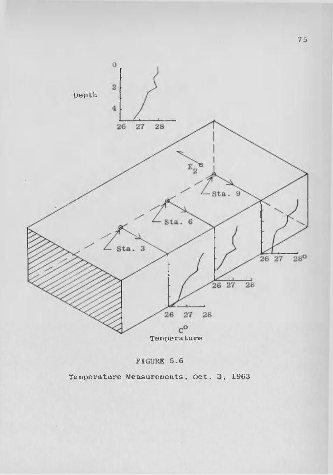
a tracer study (section 5.3.2) and vertical temperature measurements (section 5.2.3) made on November 1. The sampling location was 72 feet west of station 9 at sampling platform . Vertical distribution is shown inFigure 5.5.

5.2. Temperature MeasurementsRepresentative temperature profiles were difficult

to obtain. Many small channels of different temperatures had been observed during the construction of the sampling

Depth

70

Water surface0

I1

2 *

3 1

4*

25 30 35 40 45 50—3Coliform Density, Colonies/ml xlO"

FIGURE 5.2Coliform Profile, Station 3, 1030, Aug. 9, 1963

Depth

71

Water Surface0

V

2 *

3’

4 *

5*20 30 403525 45

Coliform Density, Colonies/ml xl0-3

FIGUhE 5.3Coliform Profile, Station 9, 1030

August 9, 1963

Depth

Water Surface0

Thermocline

2 *30* NW Effluent

3 *

4*

5*10 155 20 3025

—3Coliform Density, Colonies/ml xlO-

FIGURE 5.4Coliform Profile, Station 9, 1600, Aug. 9, 1963

Depth

V -

2 * -

4* -

5’ I—30

Water Surface

35 40 45 50 55Coliform Density Colonies/ml xlO™*

FIGURE 5.5Coliform Profile, E1, 1330, Nov. 1, 1963

74.platforms for the tracer study. Verification of this phe­nomena was achieved by drifting in the boat with the temper­ature probe located at a fixed position. Variations, although small, were almost always noted, especially at the influent end of the pond. This observation was further substantiated in the tracer studies where the dye patterns, when visible, exhibited extremely random movement.

5.2.1. Measurements, October 3, 1963As a result of operational difficulties during the

early weeks of September, the primary pond was taken out of service, Temperature measurements were continued as a matter of record, and sharp and well-defined thermoclines were observed (see Figure A-2). On September 20th, the flow was again resumed. It took about a week for flow equilibrium to develop because of the previous evaporative losses.

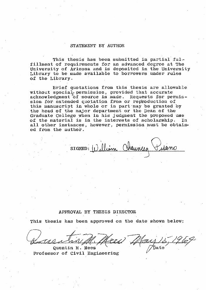
On October 3rd, measurements throughout the pond were made. The influent temperature was 29.5°C, and strong winds were noted from the Southeast. The time of measure­ment was between 1500 and 1600. Figure 5 .6 represents the temperature profiles along the length of the pond.

5.2.2. Measurements, October 5, 1963 ' . .Temperature measurements were made in conjunction

with a tracer study (section 5.3.1) on October 5. The weather was cloudy and wind movement was slight. Influent

75

Depth

Temperature

FIGURE 5.6 Temperature Measurements, Oct. 3, 1963

76and effluent temperatures were 29.5°C and 23°C respectively. Figure 5.7 shows the temperature profile taken at station 3.

5.2.3. Measurements, November 1, 1963Temperature measurements, coliform density deter­

minations, (section 5.1.3), and a tracer study (section 5.3.2) were conducted on this day. The weather was generally overcast and Southeasterly winds were generally mild. In­fluent and effluent temperatures were 26.8°C and 2Q°C respec­tively. Measurements at each station were taken with the Foxboro Portable Indicator and are presented in Figure 5.8.

5.2.4. Influent Area Study, February 20, 1964A study of the temperature variations in the

immediate influent area was made on February 20. The weather was clear and extremely gusty winds blowing from the South­east precluded extensive sampling. The influent temperature was 16°C at the flume. Figure 5.9 shows a plan view of the profile locations- as well as the corresponding vertical pro­files . It was noted that the influent was clearly boiling to the surface.

5.2.5. Influent Area Study, March 12, 1964Further investigation of the influent area was con­

ducted on March 12th. The influent temperature at the flumewas 17,5°C. Gusty winds were blowing from the Northwest.

Depth

77

Water Surface0

V

3’

4’

28 3024 26 3222Temperature °C

FIGURE 5.7 Temperature Profile

Station 3, Oct. 5., 1963

78

Sta. 6

Sta. 3

Temperature C

FIGURE 5.8 Temperature Measurements

Nov. 1, 1963

Depth

tInfluent

Plan ViewWind

0

1

2

3Vertical View

414139 1210 11 oTemperature C

FIGURE 5.9Temperature Measurements in

the Influent Area, Feb. 20, 1964

soFigure 5.10 again shows plan view location and profiles,Dye was injected into the flume and a sample of pond water was taken just as the dye came into view. Its.temperature was 16.2°C . •

5.3. Tracer Studies

5.3.1. Tracer Study, October 5, 1963The first dye study was made on October, 5. (See

section 5.2.2 for related temperature measurements.)At 1218 sufficient dye to provide a concentration

of 5 ppb, in that portion of the basin preceding the sampling stations, was introduced into the flume. At 1220 the dye first appeared at the surface of the pond in two distinct patterns. Figure 5.11 represents the two dye movements."A" was observed to move faster than "B” and passed station 3 at 1235. Its surface velocity was about 6.5 feet per minute. Visibility was reduced by dilution midway between stations 3 and 6 . MB" moved to the west side and then rapidly disappeared.

Figure 5.12 depicts the dye profiles obtained at the sampling platforms approximately 350 feet south of the influent. The time required for the first trace of dye to reach the effluent structure was 2 hours. Recovery at the effluent is also shown.

Depth

81

WindInfluent Pipe

Plan View

0

1

Profile View2

3

418°C8 10 12 14 16

o;Temperature C

FIGURE 5.10Temperature Measurements in the Influent Area,

March 12, 1964

North

Sta. 6

no longer visible

Sta. 3

6 ,5f/win

- disappears

Influent

FIGURE 5.11

Visible Dye Movements, Oct. 5, 1963

$3 /

4 - l x

1700

Samples

laao

i5“ -

tn ^Platforms •d_J\FMFIGURE 5.>1

' lleii- atng Platforms

*• Ea andr-'xTl-

845.3.2. Tracer Study, November 1, 1963

In conjunction with the temperature measurements (section 5.2.3), a second tracer study was conducted on November 1. In view of the previous work, differential sampling was performed only at the most easterly platform,

. It was anticipated that reduced sampling would minimize the mixing due to rowing. At 1442 the dye was placed in the upstream manhole. The flow rate at this time was 0.178 million gallons per day. The theoretical detention time of this basin for this flow would be about 18 days.

Figure 5.13 shows the general patterns of visible dye movements . The dye passed station 3 at 1510.. This represents a surface velocity of about 4 feet per minute. Mild Southeasterly winds were observed at this time.

Improper estimation of the arrival time at the sampling station led to a partial pickup of the wave of dye. No positive samples were taken at the effluent; how­ever, it was estimated from the time required to reach the sampling platform that dye would pass through the basin in 4-1/2 hours. Figure 5.14 represents the data obtained in this study.

5.3.3. Effluent Study on November 20, 1963An effort to determine the relative percentage of

dye passing through the basin as time progressed was made on November 20. Dye was introduced into the basin at 0955.

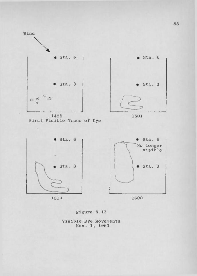
\• Sta. 6 e Sta. 6

• Sta. 3 • Sta. 3

o _ r~ " '-/o

1458 1501First Visible Trace of Dye

• Sta.

• Sta.

1510

No longer visible

Sta. 3

1600

Figure 5.13Visible Dye Movements

Nov. 1, 1963

86

V

2 *

3 f

4*

5*100 5

ppb 1830 1840

1 *

2 *

3*

4’

51100 5 1050

1850 1900

FIGURE 5.14Dye Profiles at

Sampling Platform , Nov. 1, 1963

87

The influent and effluent temperatures were 24°C and 13°C respectively. At the time of injection the wind was blow­ing very strong from the Southeast. The flow rate into the pond was 0.134 mgd. Figure 5.15 shows the visible dye movements.

Sampling began at the effluent at 1553 and continued to 2240. Figure 5.16 represents dye recovery, wind movements, surface water movements, and samples taken from other loca­tions in the pond. The peak of wind movement, occuring at 1930) represents severe gustiness which caused large quanti­ties of debris to be blown in from a near-by land fill.

Assuming that inflow equalled outflow, only 1% of the total quantity of dye injected was accounted for during the sampling period. On the following morning heavy absorption of dye by floatable solids was noticed at the Northwest corner of the pond. The bank was stained about 4 inches above the water level.

5.3.4. Aeration-Tracer Study, November 22, 1963On November 22, the first corrective measures were

initiated. The compressor was started at 1500 and was operated through the night and the following day. This procedure was adopted to insure equilibrium of the flow currents described in section 3.3.

Air was supplied to the diffusion tubing at 9 cubic • feet per minute, 5 psig, and 140°F. This imparted an

Wind

11/min .

Influent

Figure 5.15 Visible Dye Movement

Nov. 20, 1963

Tracer

Dye

10 _ 89

01500 1700 1900 2100 2300

Time of Sampling at the EffluentS . Dyke

1 2 ppb 1 2 ppb1902

Sta. 6

1905

Sta. 3

19ppb 1 2 ppb 17-17301730 1902 13-1905

N . Dyke Samples at other locations

Time Wind Directior Magnitude095015501700183019302 1 0 02 2 0 0

South East South East NoneSouth East South South None

5-10 mph 5-10 mph2-5 mph 15-20 mph 5-10 mph

Wind Direction and Estimated Magnitudes

15’min_

Wind

Surface Movement at 1600

FIGURE 5.16 Tracer Study, Nov. 20, 1963

90average volume of 0.05 cfm at the above stated conditions to each foot of pond width. Sufficient pressure could not be maintained in the last 30 feet of tubing due to excessive losses . A split-feed flow might have eliminated this problem.

At 1325 on November 23 dye was injected into theupstream manhole. Influent and effluent temperatures were23°C and 13°C respectively; the flow rate at this time was 0.156 mgd; and the wind was blowing very strong from the Southeast. Ambient temperature was about 48°F and reached a low of 39°F during the later sampling operation.

Figure 5.17 shows the general development of the visible dye movements. The wind effect should be noted in Figure 5.18. This photograph, taken from the east dike, corresponds to sketch (c) of Figure 5.17. It should also be noted that aeration in this area was the heaviest, beingclose to the source. Where the aeration was sufficient, aclear unmistakable .barrier was formed . Figure *5.19, -corres­ponding to sketch (d) was taken from the north bank at the centerline of the pond. Little visual effect was noted on the most westerly 30 feet because of the insufficient aeration. However, the quantity passing through this reach Was small in comparison to the movement on the east side of the pond. The dye was not visible beyond station 3 within an hour.

91Wind

e Sta. 3

Diffusion Piping

(a) (b)

# Sta. 3

(c)

# Sta, 3

(d)

FIGURE 5.17 Visual Dye Movements

Aeration - Tracer Study - Nov. 23, 1963

FIGURE 5.18Dye Movements

Aeration-Tracer Study Nov. 23, 1963

FIGURE 5.19Dye Movements

Aeration-Tracer Study Nov. 23, 1963

94Figure 5.20 shows the dye profiles at the sampling

platforms and at the effluent structure. Complete traverse coverage was not attempted in an effort to minimize mixing due to rowing. The first trace of the dye at the effluent was recovered in 5-1/2 hours. The theoretical detention time for the flow rate mentioned above was about 2 0 days.

5.3.5. Aeration-Tracer Study on February 21, 1964On February 21, the second aeration-tracer study

was conducted. Compressor operation was begun, and 12 CFM of air was delivered at 14 psig and 140°F. Air was supplied to the 15 foot diameter circle at a rate of 0.25 CFM for each peripherial foot. -

At 1404 the dye was introduced into the upstream manhole. The temperature of the influent was 18°C , (See section 5.2.4 for temperature measurements in the influent area) and flow into the pond was 0.288 mgd. This corres­ponds to a detention period of 10-1/2 days. Slight wind movement was noted from a Northwesterly direction.

The dye moved radially from the aeration circle somewhere beneath the surface, and the major portion of the dye was observed to/move down the centerline of the pond. Figure 5.21 represents the condition three minutes after the dye was first observed. Figure 5.22, showing the subsurface; movement just beyond the aeration circle was

m>Fi rTPTR “.

w4 m

dm

ipe+-

FIGURE 5.21Dye Movements

Aeration-Tracer Study Feb. 21, 1964

FIGURE 5.22Subsurface Dye Movements Aeration-Tracer Study

Feb. 21, 1964

98

taken two minutes later„ The dye passed station 3 at 1419. Its velocity was approximately 10 feet per minute.

Dye profiles taken at the sampling stations and at the effluent are shown in Figure 5.23. The time for first positive recovery at the effluent was about 5-1/4 hours.

:v J "

1>

: - : : > 14luent 3amp

1910 x !>r(-

1505

r>ftX"

1510i M 1620

0ORB 5v23e Prof

I -XI > J X

xkf' ^"Xl X

|S -' X: r<4 <s+X k c x ^ x i^ ':

Chapter 6

Discussion of Results

6.1 Coliform Bacteria

6.1.1. Coliform Density in Effluent Study, August 1, 1963 The results of the effluent study (section 5.1)

appear to confirm the 1962 tracer study (section 3.1.1); however, in view of investigations by others, this may not be the case. When the higher counts were noted, it should be observed that (1 ), ambient temperature had cooled the surface of the pond (see Figure 5.1) thereby causing convectional mixing, and (2 ), the sun had set and photo- cynthesis had ceased, production of speculated coliform-toxic substances by the algae may have reduced the counts

' Iin the upper layers during the hours of sunlight. (2 0 )(2 1 ). If this were the case, then the increase observed was possibly a natural incident occuring in diurnal fashion.This would not eliminate the possible existence of high- count stratified layers, since there is substantial evidence that these toxins may not exist. (22)(23)(24). Furthermore, if they do exist, their effect and production rates during the respiration period are not known.

—100 —

101Until more definitive criteria are established as

to the primary cause of colifonn die-off, this study, al­though interesting, must be regarded as inconclusive evidence of short-circuiting.

6.1.2. Vertical Coliform Density Profiles, August 9, 1963The data from Figures 5.2 and 5.3 when averaged and

combined with effluent density data shown in the appendix produce an interesting plot on log-log paper. The resulting straight line shown in Figure A.3 would seem to indicate that the die-off rate assumes a constant value. Because of the highly variable nature of the microbial world, more data would be needed to substantiate this observation.

Comparison of the relative densities of Figures 5.3 and 5 *4 seems to provide supporting evidence for the presence of algae-produced toxins. Assuming that a turnover period had taken place, diluting the 2.4 foot level with the top two feet, in Figure 5.4, a density of approximately 17,000 colonies/ml would result. This would approximate the increase observed at the turnover period during the effluent study.

It should be noted that the surface temperature was about 38°C and that a sharp thermocline existed. The temper­ature of the incoming flow during this project and during

otwo years of previous investigations was 31 C . A tracerstudy''would .have :-decided .'the- question. .Unfortunately the tracer technique had not been perfected at this time

6.1.3. Coliform Study, November 1, 1963The profile shown in Figure 5.5 would seem to provide

conclusive evidence of short-circuiting. Comparison of the overall densities of Figure 5,4 and Figure 5.5 should be noted. Algal cells were present in the pond at this time. Temperature measurements (section 5.2.3) and a tracer study (section 5.3.2) confirm these results,

6 .2 Temperature Measurements

6 .2.1. Temperature Measurements, October 3, 1963Temperature measurements made on October 3 indicated

that stratification had taken place. The existence of thiscondition is supported by the profiles at station 6 andsampling platform Eg, Figure 5.6. An increase in temperatureexisted at approximately the two foot level in both cases.Temperatures at E were about a degree warmer than those2observed at station 6 . Five conditions should be emphasized in connection with this series of measurements: 1 ) thetemperature of the influent was 29.7°C; 2) a small vertical temperature differential existed; 3) the pond was generally cooler than the influent; 4) . a strong wind was blowing from the Southeast; 5) an increase in temperature was noted at the two foot level. The later condition deserves further consideration. Its existence would suggest that the pond acted as a heat sink for the influent sewage, causing it to

103

lose its initial "temperature-density" identity. As it cool­ed, selection of a "salinity-temperature-density" level was made where it moved by a natural current gradient or possi­bly as the result of accentuation or control by wind action.

It should be noted that at Eg the surface tempera­ture was the same as the temperature at the two foot level. The existence of stratified flow was therefore unquestion­able; however, movement at two elevations was possible. Identification of the liquid flowing at either level by means of temperature measurements would be precluded, It is conceivable that the lower level could have resulted from an undercurrent movement caused by the wind and have originated as a surface layer warmed by solar radiation.

6,2.2. Influent Area MeasurementsFigures 5.9 and 5.10 show the rapid cooling of the

sewage within a few feet of the influent pipe. Curve (c), Figure 5.10 indicates the development of a warm strata below the surface. The wind effect in both cases should be noted.

6 .3. Tracer Studies. )

6.3.1. Tracer Study, October 5, 1963Temperature measurements and dye concentrat ion ob­

servations on October 5 conclusively proved the existence of severe short-circuiting. No winds were present during

104the sampling operation, and.sewage appeared to move across the surface by means of a surface gradient. Figure.5.7 shows a well-defined temperature stratification with sur­face temperature approaching that of the influent sewage.The dye profiles of Figure 5.12 show-the stratified upper layers with predominant movement on the east side. This verified visual observations shown in Figure 5,11.

It should be emphatically noted that the first recovery of dye was noted at the effluent in two hours. No flow measurements were made at this time. Assuming the maximum rate observed in this project, 0.288 mgd (section 5.3.3), the theoretical detention time would have been about 10.6 days. This means that the actual detention time was approximately l/125th of the theoretical detention time.

6.3.2. ■ Tracer Study, November 1,. 1963The second tracer study conducted on November 1 con­

firmed the October 5th results. Figure 5.14 shows the dye recovery at the sampling p l a t f o r m . , 3-1/2 hours, after the dye was introduced into the pond. Temperature measurements shown in Figure 5.8 establish the presence of warm upper layers. Coliform counts, Figure 5.5, taken at the same location definitely show the movement of potentially danger­ous untreated sewage. Again, careful note should be made, of the'effects of a slight wind blowing from the Southeast.

1056.3.3. Effluent Study, November 20, 1963

The effluent study on November 20 conclusively estab­lished the validity of the two previous studies. The dra­matic effect of wind action on surface movement is shown in Figure 5.16. Surface velocities of 15 feet per minute were observed during a heavy wind. A unit volume of incoming sewage could traverse the entire length of the pond in slightly over thirty minutes. At this rate the basin would perform only as a poorly-designed sedimentation basin.

6.4. Aeration-Tracer Studies

6,4.1. Aeration-Tracer Study, November 22, 1963The profiles shown in Figure 5.20 indicate that the

aeration system only partially mixed the stratified upper layers. The last sampling operation at 2400 showed that a uniform concentration throughout'the depths had been attain­ed . In section 3.3 it was noted that the region of influence of the aeration system would tend to increase with time Although this would seem to indicate that the last readings revealed a more efficient mixing, it must be emphasized that the compressor had been operating for about a day prior to the introduction of dye. Equilibrium should have been reached, If this were true, then the final readings showed the minor portion of the dye that had been effected by the aeration. Only a second wave of dye would answer this question. v

1 0 6

Flow measurements during this sampling period indi­cated a theoretical detention time of approximately 19 days. Since the time of first recovery at the effluent (5-1/2 hours) compared with the previously noted times, no sig­nificant increase in detention time can be attributed to the aeration system.

Two observations may be drawn from this experiment:1 ) insufficient mixing of the stratified flow occured; 2 ) the supposed mixing action of the wind was actually detri­mental to the air-induced mixing action.

Baines (25) contends that mixing by aeration should be rather effective. His relationship shown in section 3.3 indicates that the amount of entrained water should be pro­portional to the square, root of the air-flow rate. This is the extent of quantitative criteria available for this type of a problem,

Using Abraham and Burgh’s equation shown in section3.4.1.2, and assuming a condition where underflow strata exist, an air-flow rate of 0 . 1 2 cfm/foot would be needed to mix a stratified layer whose density differed by 4 x lO-^ grams/ml from that of the pond water. This was about twice the quantity of air supplied in this study. In the subse­quent experiment with the circular aeration system, 0.25 cfm/foot was used.

1076.4.2. Aeration-Tracer Study, February 21, 1964

The tracer profiles of the second aeration study shown in Figure 5.23 present an anomaly. Before aeration had begun the influent was clearly visible boiling to the surface. This same observation .was made one day earlier when temperature measurements were conducted in the influent area (section 5.2.4). However, after the dye was introduced, it was visually observed moving somewhere beneath the sur­face. An initial strong movement at the two foot level was detected at the sampling platforms. Consideration of two facts might explain this phenomena: 1 ) no algae had beenpresent in the pond for about two months; 2 ) at the lower- - temperatures the thermal effect on density is slight. The sewage, although warmer, may have been denser than the fluid in the pond. Examination of drawing (c), Figure 5.9 shows some indication of this possibility. Potential support of this explanation is also evidenced in an earlier study by Mees (11), when it was found that the total solids content of the influent raw.sewage was approximately 50 mg/ 1 greater than that of the heavily algal laden pond water which in­corporated a potential slight negative buoyancy into the system.

No movement can be attributed to wind action because, of its absence. , The aeration system, as in the first case, failed to mix the stratified flow. Again, an insufficient quantity of air may have been the problem.

108Using Schmidt’s notion of stability described in

section 2.8, an opposite view might be taken. Using the volume of flow per day and the influent and pond temperature (assuming the density of the influent remained constant), the amount of work that would have to be exerted in one day to thoroughly mix the warm stratified sewage would have been 1 0 , 0 0 0 foot-pounds for the conditions existing during the first aeration study. Because of the unknown water depth-salinity variations that existed during the second aeration study, calculation of work required for mixing the observed strata would be impossible. However, this value should not be substantially different from the amount needed for the first study.

The energy exerted by the aeration system might be calculated in the following manner:

.e « qhgrlE: energy in ft-#/min.q: flow rate expressed as efm/ft of aeration tubingh: depth of waterr: density of water§ • acceleration of gravity1 : length of aeration tubing

In the first study 2800 ft-#/ minute was exerted on the water by the aeration system. In the second case, 2900 ft-#/minute was supplied. The notion of an efficiency of energy transfer must be considered. Direct equation of the energy needed and that exerted is not possible. Evaluation

109of a thermal mixing rate is a thermodynamics problem and is beyond the scope of this thesis. However, assuming a very small efficiency of energy transfer, it would.seem reason­able to conclude that the energy supplied far exceeded the energy required for adequate mixing.

Perhaps consideration of the method of energy dis­persal rather than the quantity of energy exerted might ex­plain the, .observed failures. In both cases aeration was only attempted in the influent area of the pond. Had a num­ber of aeration lines been placed throughout the length of the pond, the results might have been different. A continu­ing breakup of any type of stratification would seem to be highly desirable. A number of cells would have definitely retarded the effect of wind movement.

Chapter 7

CONCLUSIONS AND■RECOMMENDATIONS.

7.1 General ConclusionsIt was found in this project that severe short-

Icircuiting existed during the winter and autumn seasons . For the summer months insufficient data precluded a similar con­clusion.

For the detention periods observed, sedimentation and digestion of settleable solids would take place; however, removal of dissolved and suspended solids along with accept­able bacterial reductions would be questionable.

Natural stratification aided by wind action was responsible for the rapid movement of the generally buoyant raw sewage. It must be carefully noted that wind need not be present for short-circuiting to exist. However, wind may drastically accentuate the rate of movement initiated by existing temperature-density differentials. Benefits of oxygen replenishment and influent mixing by wind action must be balanced against the additional impetus for movement. Little would be accomplished when a waste is placed in a favorable environment for only a small fraction of the time needed to accomplish the desired treatment.

The installation under study is a very ineffective means for eliminating certain pathogens that may enter the basin. This conclusion is based upon consideration of the following three facts: 1 ) E . histolytica, causative agentof amebic dysentery, can remain viable in raw sewage for 6

days at 25°C (39); 2) two days are required to completely settle cysts through a water depth of 5 feet at 25°C (see section 3.2); 3) for the particular time of year investi­gated, detention times ranging from 1/12 to 1/4 day were found to exist. If a waste containing this organism entered this treatment unit or any other similar type of installa­tion experiencing short-circuiting, the fluid leaving the basin would be potentially dangerous.

The use of air diffusion as a means pf mixing the stratified flow was found to be unsatisfactory for the par­ticular geometric configurations used.

7,2. RecommendationsFrom the observations made in this study, the follow­

ing items.are presented for consideration in the design of geometrically similar stabilization ponds:

1) Influent flow should be introduced into the basin through a number of hydraulically balanced inlets. Ideally, flow should be introduced along the entire transverse dimension. Efficient dispersal and rapid elimination of

112possible density variations should be the keynote to inlet design.

2) Effluent piping should be constructed with maximum flexibility for selective draw-off, A thorough understand­ing of seasonal variations of water movement in a lake ora pond should be fundamental.

3) Orientation of a pond site should be perpendicular to the direction of the prevailing wind. Construction of windbreaks may be desirable.

4) Equalization of influent temperatures should be practiced when feasible. This may take the form of recycling portions of the treated waste with the raw sewage in an ef­fort to minimize possible temperature-density differentials.

7.3, Suggestions for Future StudyThe author believes the following areas are worthy

of additional investigation:1) Determination of the cause for colifonn bacteria

die-off within the various environments that exist within a stabilization pond.

2) Different shaped basins should be studied in an effort to utilize the design volume more effectively. It was observed in this project that utilization of the influ­ent portion of the pond by the incoming sewage was poor.

1133) Placing aeration tubes parallel to the axis of flow

as a means of mixing a basin should be investigated. From this configuration it is conceivable that a spiral motion would result. This type of a flow pattern has been success­fully used for a number of years in the activated sludge, process .

4) In any future tracer studies conducted on either a prototype or model basin, continual dye application and long­term effluent monitoring is strongly recommended.

APPENDIX

Absorbance

114

.3

.2

1

.0

.9

8

I--Time Base -~*i7

6

5 Last visible trace of

First visible trace of dye

4

30 2 4 6 8 1 0

Time (minutes) of Sampling at the Flume

FIGURE A .1Establishment of

Time Base for Dye Injection Nov. 20, 1963

115

0*

2 ’

3*

4’

5*28 29 30 31 32 33 34

Temperature °C

FIGURE A.2Temperature Profile, Station 9, 1600

September 16, 1963

116

100

50 Station 3>»i

Station 9

Effluent

5010510Process time (days)

FIGURE A.3Coliform Bacteria Reductions as a

Function of Process Time, 1030, August 1, 1963

LI ST->©B:SBEFEBENCES

1.

2 .

3.

A.

■5.

6 .

7 .

8.

9.

10.

11.

12.

Fair, G. F . and Geyer, J . C ., Water Supply and Waste Disposal, 1st Ed., John Wiley and Sons, Inc.,New York, 1954.

United States Public Health Service, The Santee Recreation Project, U . S. Dept, of HE & W,Ban Francisco, California, 1963.

Hutchison, G . E ., A Treatise on limnology, 1st Ed.,John Wiley and~Sohs7 I he'I", ' 'New York” 1957 ,

Birge, E . A ., "The Work of Wind in Warming a Lake," Transactions of Wisconsin';Academy of Sciences, .Arts, and Letters, 24:363 (T9i'4T ' ■

Ruttner, F ., Fundamentals of Limnology, 2nd Ed., University of Toronto Press, Canada, 1953.

Standard Methods for the Examination of Water and Wastewater, American Public Health Association, American Water Works Association, and Water Control Feration, 10th Ed., Waverly Press, Baltimore, 1955.

Kelly, S., Winsser, I., and Winkelstein, W ., Poliomyetis. and other Enteric Viruses in Sewage, American Journal of Public Health, 47:72-77, 1957.

Glfsyna, E . F . and Hermann, E . R., "Waste Stabilization Ponds," Journal of Sewage and Industrial Wastes, 30:973, T95F: :

Tsivoglou, E . C ., "Field Use of a Radiotracer in Sewage Oxidation Pond,” Journal of Sewage and Industrial Wastes,28:120, 1955!

Mery, R. C ., Merrell, J. C., and Stone R ., "Investiga­tion of Primary Lagoon Treatment," Journal of Sewage and Industrial Wastes, 29:117^ 1957.

Mees, Q . M ., "Survival of Pathogens in Sewage Stabiliza­tion Ponds," Unpublished.

Offutt, A. C ., Poole, B. A., and Fassnacht, G. G.,"A Water-Borne Outbreak of Amoesiasis," American Journal of Public Health, 45:486, 1955.

—117 —

11813.

14.

15.

16.

17 .

18.

19.

20.

21 .

22.

23 .

24.

Cram, E. B ., "Effect of Various Treatment Processes on Survival of Heliminth Ova and Protozoan - Cysts in Sewage, " Sewage Works Journal, 15:1119, 1943.

Chang, S. L ., "Sedimentation in Water and the Specific Gravity of Cysts of Entamoeba histolytica," American Journal of Hygiene, 49:186, T9451 -

Newton, W. L ., "Observations of the Effects of Various Sewage Treatment Processes upon Eggs of Taenia saginata," American Journal of Hygiene, 49:166, 1949.

Tangmuir, I., "Surface Motion of Water Induced by Wind," Science 87:119-123, 1938.

Olsen, F . C., "The Currents of Western Lake," Abstraction from Thesis, Ohio State University, 62:419-424, 1952.

Kenlegan, G. H . ,. "Wind Tides in Spall Closed Channels,"Journal of Resources for Natidital Bureau of Standards, 46:358-331, 1951. ~ : '

U. S. Department of Health, Education, and Welfare. A joint report with the North and South Dakota Departments of Health. Stabilization Ponds in the Dakotas, 1957.

Caldwell, A. C ., "Sewage Oxidation Ponds - Performance, Operation, and Design," Sewage Works Journal,18:433, 1946. ~ "

Neel, J . K . and Hopkins, G. H., "Experimental Lagooning of Raw Sewage," Sewage and Industrial Waste Journal, 28:1326 ,' 1956. ..'; '' ; “

• Towne, W .'W ., Bartsch, A. F ., and Davis, W . H ., "RawSewage Stabilization Ponds in the Dakotas," Sewage and Industrial Wastes Journal, 29:377, 1957.

Oswald, W. S. and Gotaas, H. B ., "Photosynthesis inSewage Treatment," Journal of Sanitary Engineering Division, American Society ofCivil Engineers, BT:'6867T93F:------ : : “

Smallhorst, D . F ., Walton, B . N ., and Meyers, J., The Design and Application of Oxidation Ponds,” Public Works, 84, 12:89, 1953.

11925.

26.

27 .

28.

29.

30.

■31.

32.

33 .

34.

35.

36.

Baines, W . D ., "On the flow of Water by a RisingColumn of Air Bubbles, Proceedings of the Interna­tional Association for Hydraulic Researchj 8 th Congress , 2:7-1), 1959.

Straub, L . G ., Bowers, C . E ., and Tarapore, Z .S ., Experimental Studies of Pneumatic and Hydraulic Breakwaters, St. Anthony Falls Hydraulic Laboratory, Technical Paper No. 25, Series B , 1959.

Taylor, Sir Geoffry,- "Action of Surface Currents Used as a Breakwater," Proceedings of the Royal Society of London, Series IT, 231:468, 1955.

Green, J ., "Pneumatic Breakwaters to Protect Dredges," Journal of Waterways and Harbors Division, American Society of Civil Engineers, 87:67, 1961.

Evans, J. T ., "Pneumatic and Similar Breakwaters," Proceedings of the Royal Society of London,Series A, 231:457-466, 1955. -

Larson, I., Pneumatic Barrier Against Salt Water Intrusion," Journal of Waterways and Harbors, American Society "of Civil Engineers, 86:49, 1960.

Abraham, G. and Burgh, P.v.d., Reduction of Salt Water Intrusion Through Locks by Pneumatic Barriers,Delft Hydraulics Laboratory, Pbuiication Ko. 28,1962.

Williams, G. P., "A Study of Winter-Water Temperatures and Ice Prevention by Air Bubbling," The Engineering Journal, 44,3:79-84, 1961.

Vallentyne, J. R ., "Principles of Modern Limnology," American Scientist, 45, 3:218-244, 1957.

Brewer, M , C ., "The Thermal Regime of an Artie Lake," American Geophysical Union, Transactions, 39, ^7S-58'4; 19" 5 8 .----■------

Hurwitz E .,"Conversion to an Aerated Lagoons Extends Pond’s Life," journal of Water and Sewage Works,1963, . ' " ' “ “ 1 ~

Proceedings of the Symposium on Air Bubbling, Ottawa,' National Research Council of Canada, Associate

Committee on Soil and Snow Mechanics, Technical Memorandum No.-70, 1961.

12037. Feuerstein, D . L . and Selleck, R. E . ’’Tracers for

Dispersion Measurements in Surface Waters Journal of the Sanitary Engineering Division, American "Society of CiviT Engineers, 39, SA4,:5,loos. ; ; ; 1

38. Rabinowitch, E. I., Photosynthesis, Vol. 2, Part 1.Interscience Pbulishers, Inc., New York, 1951.

39. Chang, S. L, ’’Survival Of Cysts of Entamoeba histolytica in Human Feces under low Temperature Conditions,

- American Journal of Hygiene, 61:103-120, 1955.