Embed Size (px)
Citation preview

Thermal persistence in E. coli and
the heat shock response
Jonathan Kang
Thesis advisor: Prof. Daniel Weinreich
Second reader: Prof. David Rand
Ecology and Evolutionary Biology
A thesis submitted in partial fulfillment
of the requirements for the degree
of Bachelor of Science with Honors
in Applied Mathematics – Biology
at Brown University
April 2012

TABLE OF CONTENTS
Abstract 1 Introduction 1 Persistence: An overview 1
The mechanism behind antibiotic persistence 5
The connection to thermal persistence 8
The heat shock response: An overview 10
The rpoH gene and the synthesis and regulation of σ32 11
The relationship between thermal persistence and the heat shock response 14
Materials and methods 16 Experimental protocol 16
Analysis of data 21
Results 24 Preliminary experiments 24
Main experiments 25
Model selection using AIC 27
Estimation of parameter values 28
Incubation time and the size of colonies 29
Heritability of the persister phenotype 32 Discussion 34 The rate of death of KY1429 over a relatively high temperature range 34
The choice of temperatures for both strains 35
Interpretation of the AICc values 37
Comparison of the various estimated parameters between both strains 39
The value of p for both strains 39
The slower growth of colonies in samples under prolonged thermal stress 41
Future directions 42 Are thermal persisters and antibiotic persisters the same subset of cells? 42
How are persisters related to viable but non‐culturable cells? 43
Acknowledgements 45 References 46

1
ABSTRACT
Persistence is a phenomenon whereby a genetically uniform population of bacteria, when
subjected to some form of stress, shows a biphasic death curve. The majority of the
population dies at a certain exponential rate, while some small fraction dies at some slower
exponential rate. Persistence is not genetic on basis, as when a cell that is identified as a
persister is regrown, it still exhibits the same characteristic biphasic death curve. The bulk
of the current literature investigates persistence in response to antibiotic stress. Previous
work in the Weinreich Lab has demonstrated that bacteria can persist against heat as well.
This project studies a potential mechanism for persistence: the bacterial heat shock
response. Two E. coli strains: a mutant with the gene that is responsible for activating the
heat shock response non‐functioning, and its direct ancestor, were subjected to thermal
stress treatments. It was found that the mutant strain still exhibited a biphasic death curve
under thermal stress, even as it lacks the mechanism to activate the heat shock response.
These findings confirm that the phenomenon of bacterial persistence is independent of the
heat shock response.
INTRODUCTION
Persistence: An overview
Bacterial persistence is a phenomenon first discovered in the 1940s, when it was observed
that the complete sterilization of a bacterial culture using antibiotics was not easily

2
attainable (Bigger, 1944). The term ‘persisters’ was coined by Bigger himself, and he used it
to describe the minute fraction of the original bacterial population which had managed to
survive the antibiotic treatment. In present terms, bacterial persistence can be described as
the condition whereby some proportion of a genetically uniform microbial population
survives exposure to a stress factor, such as an antibiotic or heat treatment (Balaban et al.,
2004). Quantitatively, persistence can be characterized by the presence of two differing rates
of cell death upon the introduction of the stress factor. The vast majority of the cells in the
population would die at a certain exponential rate, while the remaining small percentage of
the cells would die at some much slower rate. A characteristic persister death curve is
shown in Figure 1.
Figure 1 (Gefen & Balaban, 2009): An archetypal biphasic persister death curve in response to ampicillin.
The first portion of the curve represents the exponential death rate of the non‐
persister cells, and the second portion of the curve represents the slower death rate of the

3
persister cells, which in this example make up approximately 1 in 102 of the total bacterial
population. The result is a biphasic death curve that is typical of persistence. It should be
noted that presence of two separate phases is a consequence of the fact that the death rate of
the persisters manifests itself in the curve only when the non‐persisters, which die at the
faster rate, have decreased to suitably low numbers. The biphasic curve is not the result of
persister death temporally lagging behind non‐persister death, despite the fact that such an
interpretation would be consistent with the death curve as presented. Persisters do in fact
start to get killed, albeit at a slower rate, upon initial introduction of the antibiotic. The
reason why this fails to register on the overall death curve until much later is due to the
small number of persisters in relation to entire bacterial population.
It may be worthwhile at this point to recognize persistence as a phenomenon that is
distinct from two others that are commonly observed in bacteria, namely, resistance and
tolerance. A comparison of the death curves that are indicative of each mechanism is given
in Figure 2. Antibiotic resistance in bacteria is a genetically acquired trait and can thus be
passed on to subsequent generations. However, it has been demonstrated that persistence
in not heritable (Keren et al., 2004). When a sample of antibiotic persister cells that had been
washed and inoculated in a fresh medium was used to start another antibiotic assay, a
biphasic death curve was still observed. This result conflicts with what one would expect if
persistence were heritable, in which case the new death curve would be monophasic, with
the entire regrown population dying at the slower rate. Comparing the persistence and
resistance death curves, both share a common initial portion where the slopes are identical.

4
This death rate can be taken to be that of the “wild‐type” bacteria, which have the dual
property being cells that have yet to acquire resistance, as well as being non‐persisters.
Figure 2 (Gefen & Balaban, 2009): Comparison of the death curves demonstrated by
different mechanisms in response to the introduction of an antibiotic. The first antibiotic
treatment (first purple region) is followed by a period of regrowth without antibiotics
(white region) and a second exposure to antibiotics (second purple region).
It is also possible to distinguish persistence from bacterial tolerance. Tolerance can
be described as the condition by which a bacterial population’s sensitivity towards some
specific stress factor is reduced. For example, if a strain of bacteria is tolerant with respect to
ampicillin, then a larger dosage of the antibiotic is required to achieve the same killing
effect as compared to a non‐tolerant strain. Equivalently, for the same dosage of ampicillin,
the tolerant strain is killed at a much slower rate as compared to the “wild‐type”. This can
be seen in Figure 2, where the tolerance death curve is much less steep as compared to the
initial portion of both the resistance and persistence curves. Finally, an additional point to
note is that the tolerance death curve fails to exhibit the biphasic pattern that is
characteristic of persistence.
5
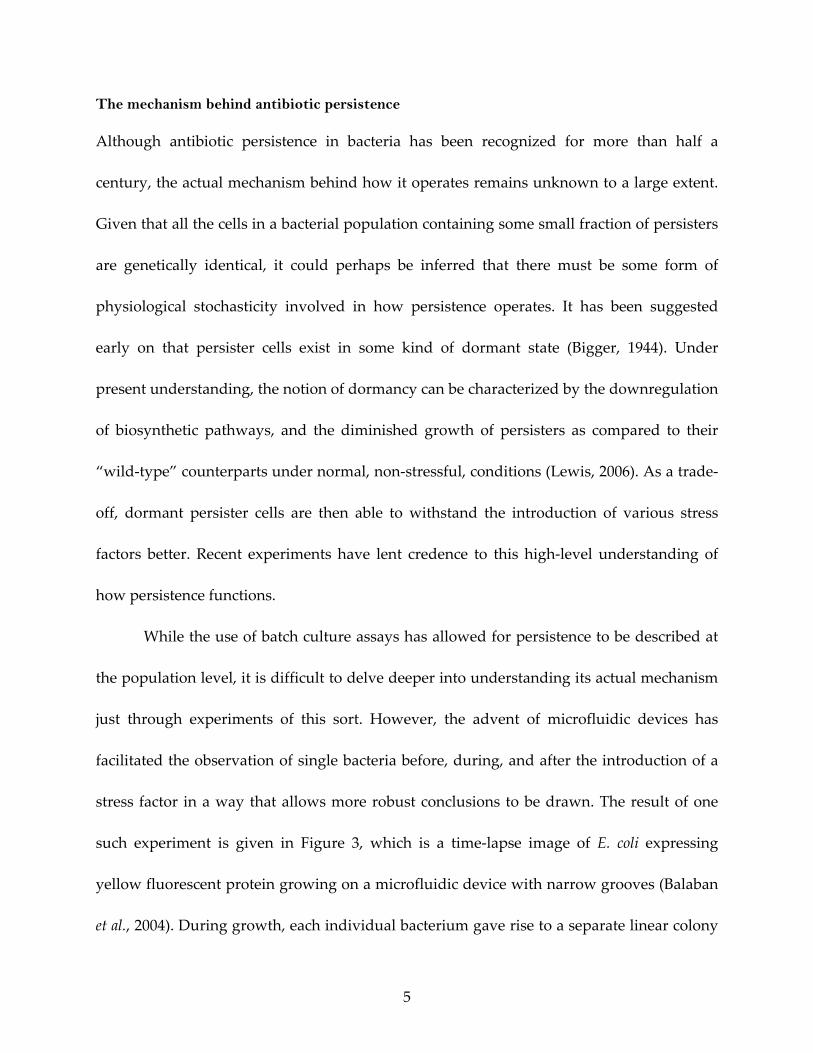
The mechanism behind antibiotic persistence
Although antibiotic persistence in bacteria has been recognized for more than half a
century, the actual mechanism behind how it operates remains unknown to a large extent.
Given that all the cells in a bacterial population containing some small fraction of persisters
are genetically identical, it could perhaps be inferred that there must be some form of
physiological stochasticity involved in how persistence operates. It has been suggested
early on that persister cells exist in some kind of dormant state (Bigger, 1944). Under
present understanding, the notion of dormancy can be characterized by the downregulation
of biosynthetic pathways, and the diminished growth of persisters as compared to their
“wild‐type” counterparts under normal, non‐stressful, conditions (Lewis, 2006). As a trade‐
off, dormant persister cells are then able to withstand the introduction of various stress
factors better. Recent experiments have lent credence to this high‐level understanding of
how persistence functions.
While the use of batch culture assays has allowed for persistence to be described at
the population level, it is difficult to delve deeper into understanding its actual mechanism
just through experiments of this sort. However, the advent of microfluidic devices has
facilitated the observation of single bacteria before, during, and after the introduction of a
stress factor in a way that allows more robust conclusions to be drawn. The result of one
such experiment is given in Figure 3, which is a time‐lapse image of E. coli expressing
yellow fluorescent protein growing on a microfluidic device with narrow grooves (Balaban
et al., 2004). During growth, each individual bacterium gave rise to a separate linear colony

6
which lengthens over time, as can be seen in the first three panels of Figure 3. When an
antibiotic (ampicillin, in this case) was introduced, most of the cells were killed, as is
evident in the fourth panel. Only a single cell, indicated by the red arrow and presently
identified as a persister, managed to survive the ampicillin treatment. When the persister
cell is traced back to the first three panels, it is clear from the weaker fluorescence that it
had experienced a lack of growth under normal conditions in the growth medium, during
which most of the other cells were actively dividing. However, after the ampicillin had been
cleared and a fresh batch of growth medium was introduced, the persister cell appears to
have left its previous state of dormancy and resumed normal growth, as can be observed in
the final two panels of Figure 3.
Figure 3 (Balaban et al., 2004): Time‐lapse experiment of bacteria expressing yellow
fluorescent protein. Times are indicated at the top of each panel in hours and minutes.
This experiment demonstrates the stochastic nature of the process by which bacteria
cells enter and leave a state of persistence. The authors conclude that the phenomenon of
persistence is associated with the heterogeneity in the growth rates of individual cells

7
within the entire bacterial population. This can be attributed to the fact that cells with
reduced growth rates will be less sensitive to antibiotics that target the cellular replication
machinery. Ampicillin, which belongs to a class of antibiotics known as β‐lactams,
functions in precisely such a manner. β‐lactams act by inhibiting the synthesis of the
peptidoglycan layer of bacterial cell walls, causing dividing cells to shed their cell walls and
fail to divide, forming instead fragile spheroplasts that are vulnerable to lysis (Fisher et al.,
2005). Dormant, non‐dividing, cells would therefore be less susceptible to ampicillin’s mode
of action, conferring them a lower death rate in its presence, and ultimately manifesting as
observable persistence.
The question then becomes how is such a stochastic transformation into and out of a
dormant state achieved. One possible approach to this problem is to perform a knockout
screen to determine if the loss of any one specific gene results in the absence of antibiotic
persisters in that particular mutant population. It was found that several different genes
might be implicated in the generation of antibiotic persisters, thus painting a picture that is
considerably more complicated than if the trait were monogenic (Lewis, 2010).
Furthermore, the screen did not produce any single mutant that completely lacked
persisters, suggesting some degree of redundancy in the mechanism for their formation
(Hansen et al., 2008). Among the genes that were identified, the majority of them are global
regulators such as DnaKJ, HupAB, IhfAB and DksA. A list of the candidate persister genes
and their pathways of action is given in Figure 4. The fact that many of these genes are
global regulators is yet another aspect of redundancy, as a global regulator can

8
simultaneously affect the expression of many different persister genes, which would all
contribute to the presence or absence of the persister phenotype (Lewis, 2010).
Figure 4 (Lewis, 2010): The various redundant candidate pathways of antibiotic persister
formation.
The connection to thermal persistence
Previous literature, as well as prior work performed in the Weinreich Lab, has
demonstrated that in addition to antibiotic stress, bacteria do persist against thermal stress
as well (Humpheson et al., 1998). Figure 5 shows the results of two sets of experiments, in
which a population of bacteria of the E. coli C strain were challenged with ampicillin and
heat respectively. A biphasic curve was observed in both cases, suggesting persistence
being in effect. One specific point to note is the time scale on the horizontal axis, which is in
hours in the case of the ampicillin assay, and minutes in the case of the heat assay. The
difference in the rate of death can be attributed to the inherent disparity in how stressful
each particular treatment is to the population. In this case, as it usually is in general, the
heat treatment eliminates the bacteria more quickly than the ampicillin treatment does.

9
Figure 5: Death curves exhibiting persistence under both antibiotic and thermal stress. The
former is due to previous work by Robin Zelman, and the latter is due to previous work by
Nicole Damari and Ayoosh Pareek.
A natural question to ask at this point is if antibiotic and thermal persistence operate
under similar mechanisms. Looking at Figure 5 again, when one traces the point at which a
death curve transitions into the second, slower, phase back to the vertical axis, that
particular value can be taken to represent the proportion of the bacterial population that are
persisters. There are then significantly more antibiotic persisters in this population than
there are thermal persisters, which would not have been the case if their modes of action
were identical. This naturally prompts one to question how thermal persistence functions,
and in what ways it differs from antibiotic persistence.
Incidentally, the DnaKJ regulator, which was found to be implicated in the
generation of antibiotic persisters, are also molecular chaperones that constitute part of a
cellular machinery for the repair of heat‐induced protein damage (Schröder et al., 1993).

10
Apart from that, DnaK and DnaJ also belong to a class of proteins known as the heat shock
proteins, which are a group of roughly twenty proteins which have their syntheses induced
by a temperature upshift. This induction of the heat shock proteins in known as the heat
shock response. The fact that the DnaKJ regulator is involved in both antibiotic persistence
and the heat shock response should prompt one to consider the arguably more obvious link
between thermal persistence and the heat shock response. This connection is strengthened
by the fact, as will be seen in the next section, that the time scale at which the heat shock
response operates (2 to 4 minutes) is comparable to that of thermal persistence (Connolly et
al., 1999).
The heat shock response: An overview
Although named as such, the heat shock response is not just triggered as a reaction to
elevated temperatures. It is also brought on by a large variety of stress conditions, including
the presence of metabolically harmful substances, as well as oxidizing conditions (Arsène et
al., 2000). In E. coli, a temperature upshift from 30 to 42°C causes a rapid, up to 15‐fold
induction in the synthesis of the various heat shock proteins, which is then followed by a
period of adaptation where the rate of heat shock protein synthesis decreases such that a
new steady state is achieved (Bukau, 1993). The major heat shock proteins are molecular
chaperones and proteases. DnaK and DnaJ, together with GrpE, constitute one of the two
major chaperone systems in E. coli, with the other being the GroE chaperone system, which
is made out of yet another set of heat shock proteins. These chaperone systems are
considered important because they make up 15‐20% of the total protein in E. coli at 46°C,

11
indicating the major role they play in cell survival in conditions of temperature stress
(Georgopoulos et al., 1994). Molecular chaperones are vital in ensuring the correct folding
and assembly of proteins. Presumably, such a function becomes even more important at
higher temperatures, as proteins become increasingly unstable and are unable to correctly
form their proper, functional structures.
The heat shock response in E. coli is positively regulated at the transcriptional level
by the σ32 protein, which is the product of the rpoH gene, and is also the heat shock
promoter‐specific subunit of RNA polymerase (Gross, 1996). σ32 is required for both the
induced expression, as well as the uninduced, basal expression of the various heat shock
genes. The cellular concentration of σ32 is extremely low under steady state conditions (10‐
30 copies per cell at 30°C), and is the limiting factor for the transcription of heat shock genes
(Craig & Gross, 1991). The heat shock response comes about as the consequence of a rapid
increase in σ32 levels, leading to an upsurge in heat shock gene transcription and the
production of heat shock proteins. Regulation of the heat shock response through the
variation of σ32 levels in the cell is a fairly rapid process, and thus allows for E. coli to
respond quickly to sudden occurrences of stress.
The rpoH gene and the synthesis and regulation of σ32
As previously described, the σ32 protein is a product of the rpoH gene. The regulation of
rpoH transcription is complex, and has only a minor effect on the amount of σ32 that is
eventually synthesized. On the other hand, the stress‐dependent changes in σ32 levels

12
appear to be much more dependent on the changing rates of translation of rpoH mRNA.
rpoH translation is repressed under steady state conditions, which accounts for the low
cellular concentration of σ32 when circumstances are favorable. However, 2 to 4 minutes
after a temperature upshift from 30 to 42°C, a corresponding 12‐fold increase in the level of
translation occurs. When the stress factor is removed, translation is once again repressed
during the shut off phase of the heat shock response, until a new steady state is reached
(Connolly et al., 1999). This system of rpoH translation control is mediated biochemically
through distinct mechanisms involving three cis‐acting elements of the rpoH coding
sequence (Nagai et al., 1991).
Apart from transcriptional and translational elements, variations in σ32 levels are
also affected by the stability of the protein itself (Connolly et al., 1999). During steady state
growth, σ32 has an extremely short half‐life of less than 1 minute. Upon a temperature
upshift from 30 to 42°C, σ32 becomes transiently stabilized at least 8‐fold, up to the point
when the heat shock response begins to get shut off. A protease that is responsible for σ32
degradation is the ATP‐dependent zinc‐metalloprotease, FtsH. FtsH is an integral
cytoplasmic membrane protein, and has an active site which shares a high sequence
homology with the conserved family of AAA (ATPases Associated with diverse cellular
Activities) proteins. The degradation of σ32 by FtsH is evidenced by the fact that in the
absence FtsH, σ32 is completely stabilized in vivo, with a half‐life of 2 hours (Tatsuta et al.,
1998). Figure 6 gives a schematic representation of the E. coli heat shock regulon, involving
the various control processes that have just been described.

13
Figure 6 (Arsène et al., 2000): The E. coli heat shock regulon, representing the biochemical
mechanisms behind the control of the heat shock response.
In addition, there is also evidence to suggest that some form of feedback inhibition is
at work in the regulation of σ32 levels. Specifically, DnaK and DnaJ, which were previously
described as heat shock proteins whose production is regulated by σ32, have the
supplementary role of regulating the activity of σ32 and preventing even more heat shock
proteins from being generated when they are not needed. This aids in the establishment of
appropriate heat shock protein levels after cells have recovered from stress treatment, and
also helps maintain the homeostasis of heat shock gene expression. The fact that σ32 activity
can be modulated in such a manner is due in part to the reversible association of DnaK and
DnaJ to σ32, which inhibits heat shock gene transcription activity (Buchberger et al., 1999).
Regulation models have proposed that the induction of the heat shock response by σ32 after
stress treatment relies of the sequestration of DnaK and DnaJ through their binding to the

14
misfolded proteins that have accumulated as a result of the treatment. Once such proteins
have either been refolded or degraded, DnaK and DnaJ become unbounded, and can then
bind to σ32 and aid in the shutting down of the heat shock response (Craig & Gross, 1991).
The relationship between thermal persistence and the heat shock response
Bacterial persistence and the heat shock response appear, at least initially, to be distinct
processes that operate independently of each other. Although they are both mechanisms
that facilitate self‐preservation when bacteria undergo stressful conditions, their seemingly
differing modes of action do not lend credence to the suggestion that the persistence can be
explained by the heat shock response. While persistence has been traditionally studied in
the context of antibiotic stress, past results from the Weinreich Lab have indicated that
persistence does in fact also manifest itself under conditions of thermal stress, albeit, as seen
previously, on a different time scale. Going back to the question raised earlier, it would be
interesting to see if any connections can be drawn between thermal persistence and the heat
shock response. In the broadest sense, the issue then is if the action of the rpoH gene and σ32
protein, which is responsible for the production of heat shock proteins and the initiation of
the heat shock response, is also ultimately the cause of thermal persistence observed.
There are several reasons why this hypothesis deserves further study. First, it is clear
that the heat shock mechanism as mediated by the rpoH gene and σ32 protein constitutes a
complex regulatory framework, with controls at the transcriptional and translational levels,
as well as factors such as protein stability and feedback inhibition all playing a part in the
fine regulation of the process. It should also be noted that apart from DnaK and DnaJ,

15
under conditions of stress, σ32 also induces the expression of many other heat shock genes.
It is thus not inconceivable that persistence can arise as a consequence of the action of some
specific component within the totality of a complicated system such as this. A further point
to make in this regard is that persistence has been shown to exist under at least two
different stress conditions (antibiotics and heat). Since the heat shock response is also
activated as a reaction to a wide variety of unfavorable circumstances, there is basis to
conjecture that both phenomena could be connected.
On top of general theoretical considerations regarding the complexity of the heat
shock response, there are also reasons borne out by actual experimentation to consider
persistence and the heat shock response as being related processes. As pointed out earlier, a
knockout screen that was performed to identify the genes that are ultimately responsible for
the persister phenotype points to the DnaKJ system, among others, as being a possible
candidate. Since DnaK and DnaJ constitute an integral part of the heat shock response
pathway, there is then reason for studying the relationship between both systems in closer
detail. Finally, results of previous experiments conducted in the Weinreich Lab have
indicated that the time taken for the bacteria death curve to switch to the slower second
phase when subjected to thermal stress is in the neighborhood of 4 minutes, which is to an
approximation the point in time when the heat shock response gets activated. Based on
these observations, a series of experiments was conducted to further explore the effect that
the activation of the heat shock response has on thermal persistence.

16
MATERIALS AND METHODS
Experimental protocol
The aim of these experiments is to find out how bacteria which lack the ability to initiate the
heat shock response react to conditions of thermal stress. Specifically, the question to be
asked is if such bacteria still exhibit the biphasic death curve that is characteristic of
persistence. To this end, two strains of bacteria were obtained from the Coli Genetic Stock
Center (CGSC) at Yale University. The KY1429 strain (CGSC#: 6934) is a heat‐sensitive
strain with a mutation in the rpoH gene, which is, as mentioned previously, the gene
responsible for producing the σ32 protein, which in turn regulates the transcription of a
variety of heat shock genes. This strain is then lacking the heat shock response. As a control,
the direct ancestor of KY1429, the MC4100 strain (CGSC#: 6152), was also obtained from
CGSC. This strain does not have a mutation in the rpoH gene, and is therefore able to
activate the heat shock response. The outcome of the thermal stress experiments on KY1429
will be compared to the same set of experiments on MC4100 so as to ensure that any
difference in results is due solely to the lack of a functioning rpoH gene in KY1429.
The experimental protocol is for the most part identical for both strains. However, as
KY1429 is heat‐sensitive, all steps involving incubation were performed at 25°C, as opposed
to 37°C for MC4100, which is the standard for most other strains of E. coli. In each run of the
experiment, a single colony of bacteria was incubated overnight in some volume of Difco
LB Broth Lennox, which varied according to how much culture was actually needed for a
particular run. Initial testing had indicated that there is no appreciable difference between

17
using cells in stationary phase as opposed to cells in exponential phase. This is in contrast to
an antibiotic assay, where cells in exponential phase, presumably because they are actively
dividing, are much more susceptible to the effects of the antibiotic as opposed to cells in
stationary phase. This is yet another reason to suspect a difference in the mechanisms
responsible for antibiotic and heat persistence. Therefore, in this protocol, the overnight
culture is not diluted and grown back up to exponential phase before being used for the
experiment.
However, because the initial killing phase thermal stress treatment eliminates a large
proportion of the bacteria present at the beginning of the experiment, using just the
overnight culture would fail to provide the full resolution of the death curves’ dynamics. By
the time the curve transitions into the subsequent, slower, phase, there would be too few
bacteria remaining to provide an accurate count. Thus, there is an additional step in the
protocol to obtain a higher concentration of bacteria. To accomplish this, the overnight
culture was placed in 50ml centrifuge tubes and centrifuged at 4000 rpm and 4°C for 20
minutes. When this was completed, the supernatant was discarded and the pellet
resuspended with 0.5ml of LB. 100μl of this concentrated culture was then dispensed into
PCR tubes. Completing this process increases cell concentration by about 100‐fold.
As a starting point, preliminary experiments were conducted over a range of
temperatures (54.8°C to 61.2°C) in order to get a general idea of what the death curves of
both strains look like within the range. The outcomes of these experiments are shown in
Figures 7a and 7b. Based on these results, the main experiments were performed, for

18
purposes of data collection, at 56.5°C and 58.5°C for KY1429 and MC4100 respectively. A
PCR machine was utilized to attain conditions of thermal stress, with the temperature of the
lid set to 85°C and the temperature of the block set initially to 20°C. The PCR tubes
containing the concentrated cells were then loaded onto the machine and the block ramped
up to the required temperature, a process that took about 10 seconds. Once the requisite
temperature was reached, timing began and the first sample (t = 0) was removed from the
PCR machine and immediately placed on ice. Subsequent samples were each removed from
the machine at one‐minute intervals, for a total duration of 15 minutes.
Figure 7a: Death curves for MC4100 over a range of temperatures.

19
Figure 7b: Death curves for KY1429 over a range of temperatures.
The next part of the protocol consists in trying to determine the number of colony
forming units (CFUs) per ml left in the culture after each specific duration of thermal stress.
Due to the fact that the culture in the PCR tube may contain a high concentration of cells, it
cannot be plated directly on a LB agar plate and still produce a countable number of
colonies. In addition, it is difficult to determine a priori the exact order of dilution that must
be performed in order for a sample that is plated to be countable. To address these
problems, a method known as spot‐titering was used. Wells in a 96‐well plate were filled
with 180μl of LB, and 20μl of the post‐experimental culture in the PCR tubes were each
placed into one of the wells, thus making a ten‐fold dilution. Following this, successive ten‐
fold dilutions were obtained by pipetting 20μl of liquid from each of those wells into a new
set of wells with 180μl of LB. This process of serial dilutions was repeated a total of nine
times. This process was facilitated by the use of a 12‐channel multichannel pipette.
20
10μl of liquid in each of the wells was then spot‐titered on a LB agar plate. Together,
they represent the full range of dilutions for each time point. The plates that contain
MC4100 samples were incubated at 37°C overnight, while those that contain KY1429
samples were incubated at 25°C for about 36 hours. These represent the minimum
incubation times, which in reality ended up being much longer as a result of circumstances
that will be described in the results section. After incubation, the colonies that have formed
on the plates are scored. For each time point, the spot where the colonies first become
countable is counted, and that number can be extrapolated to determine the original
concentration of cells in CFUs/ml.
In the initial conception of this experiment, based on the results of spot‐titering,
suitable dilutions from each time point would be plated on full plates to obtain more
accurate counts. This could only be done at least one day after the thermal stress part of the
protocol had been completed, and the samples were stored at 4°C during the intervening
period. However, it was found that plating from the day‐old samples did not produce
viable colonies. Therefore, for the actual collection of data in the main experiment, 100μl of
two appropriate dilutions (or 50μl if plating directly from the post‐experimental culture)
from each time point were plated on full plates immediately after the cells had undergone
heat treatment. The specific dilutions chosen were informed by previous spot‐titering
results. The data were then plotted onto a graph, with the x‐axis being the time exposed to
thermal stress in minutes, and the y‐axis being CFUs/ml on a logarithmic scale.

21
Analysis of data
Three replicates of the experiment were performed for each of the two strains. Due to the
fact that each replicate began with a different bacteria count, the raw data, originally given
in CFUs/ml, was first converted into percentage survival before it was analyzed. This
ensures that the data across the replicates are comparable. The first step of the analysis
consisted of applying a simple linear model to the data points, which was done using
MATLAB. The two parameters being estimated are α, the slope; and β, the y‐intercept of
the line. There is also a residual sum of squares (RSS) value associated with this regression,
which is a measure of the discrepancy between the data and the estimation model. A small
RSS value indicates a tight fit of the model to the data. This simple model serves as a
baseline to which the more complicated biphasic model can be compared against.
The second step of the analysis involved applying a biphasic model to the same set
of data points. Under this model, there are five parameters being estimated: α1 and β1, the
slope and y‐intercept of the line representing the initial, exponential, death rate; α2 and β2,
the slope and y‐intercept of the line representing the subsequent, slower, death rate; and γ,
the point in time when the first phase transitions into the second phase. A multi‐phase
linear regression was applied to fit the model to the data. What this eventually amounted to
was dividing the set of points into two segments, and fitting a simple linear model to each
segment.
Although this regression method seems to be no qualitatively different from a
simple linear regression, the presence of the γ variable renders this problem non‐linear.

22
This is due to the fact that the biphasic curve, in its entirety, is non‐differentiable at the
point of transition between the two phases. Therefore, a simple expansion upon the method
used to find a simple linear regression fit is insufficient for this purpose, and an analytic
method of solution was eschewed for a computational one. A MATLAB script has been
written for this purpose by Andy Ganse from the Applied Physics Laboratory at the
University of Washington, and was downloaded from http://staff.washington.edu/
aganse/mpregression/mpregression.html. It returns the maximum likelihood estimated fit
to the data based on a biphasic model. As with the case of fitting a simple linear model,
there is also a RSS value that is associated with this multi‐phase linear regression.
In order to show evidence of persistence in both the KY1429 and MC4100 strains, the
goodness of fit of the biphasic model needs to be compared with that of the linear model. If
the former fits the data better than the latter, then there is support for the conclusion that
there is in fact persistence. If not, a simple log‐linear death rate would then be the preferred
explanation for the observed data. Usually, when comparing models with the same number
of parameters, say, for example, two linear models, the RSS value would, by itself, be
sufficient to determine which model has the best fit. However, in this case, a model with
five parameters is being compared to a model with two parameters, with the additional
complication of the former being non‐linear. Generally, the more parameters some
particular models appeals to, the better the resulting fit will be. Yet, overfitting, which is the
situation whereby more parameters than strictly necessary are invoked by virtue of the

23
model choice, should be avoided. To accomplish this, there needs to be some sort of penalty
that comes with the use of additional parameters.
As a tool for model selection that takes into account both the goodness of fit and the
number of parameters, the Akaike Information Criterion (AIC) can be applied (Akaike,
1974). In its most general form,
AIC 2lnL 2k , (1)
where L is the maximum likelihood of the estimated model and k is the number of
parameters in the model. If the model is a good fit to the data, then the value of L would be
high. Therefore, models with low AIC values are favored over models with higher ones.
The AIC calculation can be performed for a set of models, and the one with the lowest AIC
value is deemed the most supported. The exact application of AIC to the data collected for
this project, involving the use of RSS values to calculate the likelihoods of the models, as
well as the application of a bias adjustment for small samples, is deferred until the results
section.
There are some general comments that can be made about how using AIC as a
means for model selection differs from traditional hypothesis testing, where a null
hypothesis is rejected (or not) in favor of an alternative hypothesis based on some
significance value that is calculated. AIC does not provide information about how well a
model fits the data in an absolute sense, in the way that hypothesis testing using p‐values
does. Instead, AIC compares how good different models within a set are relative to one
another. This necessarily means that models that are not present in the set are not taken into

24
account. For example, for the purposes of this project, since a triphasic model is not being
considered, AIC does not say anything about how good it is in comparison to the linear and
biphasic models. A further implication is that AIC will pick one model as estimated to be
the “best”, even if none of the models are good in the absolute sense (Burnham &
Anderson, 2002). Therefore, there should be some prior, well‐founded rationale in the
selection of the set of models. In this case, the linear model was picked because it represents
the result that should be expected if the lack of the heat shock response does indeed ablate
persistence, and the biphasic model was chosen precisely because it is how one would
observe for persistence.
RESULTS
Preliminary experiments
To identify the most suitable temperatures at which the main experiments should be
conducted, two preliminary experiments, one each for KY1429 and MC4100, were
performed, applying essentially the same protocol. Eight temperature points between
54.8°C to 61.2°C were used, and thermal stress was only applied for 7 minutes, due to space
limitations in the PCR machine. The results for MC4100 and KY1429 were given in Figures
7a and 7b respectively.
It is clear that temperature does have a significant effect on the steepness of the slope
in the initial, exponential, phase, as well as on the point in time when the death curve
transits into the subsequent, slower, phase. However, in some cases, the transition is not

25
apparent due to limitations on the resolution of spot‐titering. In addition, for most of the
curves, the slope of the subsequent phase is not readily observable, as the preliminary
experiments were terminated after just 7 minutes. As a result, no robust conclusions can be
drawn about how the steepnesses of the second phase slopes extend beyond 7 minutes.
It is also obvious that there are differences between how the collection of death
curves look in the case of MC4100 in contrast to KY1429. On a general level, MC4100
appears to withstand the thermal stress treatment better than KY1429, with shallower
slopes in the initial phase when comparing across the same temperatures. Presumably, this
is due to KY1429 lacking the rpoH gene, as that is the only genetic difference between both
strains. However, there is a case to be made that this difference as observed is actually
smaller than expected. A more detailed explanation as to why this is so follows in the
discussion section.
Ultimately, the purpose of the preliminary experiments is to help with the
identification of suitable temperatures at which the main experiments could be run. After
observing the shape of the death curves across the temperature range, 58.5°C and 56.5°C
were selected for MC4100 and KY1429 respectively. There were several considerations that
went into this decision, which will be examined in greater depth in the discussion section.
Main experiments
To ensure the robustness of the data, three replicates were performed for each strain. In
order for the results across the replicates to be comparable, the CFUs/ml value at each time
point was divided by the CFUs/ml value at t = 0 to obtain the percentage survival. Also, the

26
duration of the thermal stress treatment was extended to 15 minutes. The results for
MC4100 (at 58.5°C) and KY1429 (at 56.5°C) are given in Figures 8a and 8b respectively. In
addition, the average percentage survival for each time point across all three replicates at
each was calculated, and both biphasic and linear death curves are fitted to the set of
average points, using the techniques that were previously discussed in the materials and
methods section.
Figure 8a: Death curves across three replicates for MC4100 at 58.5°C, and the average of the
replicates. Both biphasic and linear models are fitted using the average set of points.

27
Figure 8b: Death curves across three replicates for KY1429 at 56.5°C, and the average of the replicates. Both biphasic and linear models are fitted using the average set of points.
Model selection using AIC
In the materials and methods section, a general sketch of how AIC works was given. Here,
the specifics of how this statistical approach is applied to both models under consideration
are presented. First, recall that in its most general form,
AIC 2lnL 2k , (1)
where L is the maximum likelihood of the estimated model and k is the number of
parameters in the model. Furthermore, if one assumes that all models within the set have
normally distributed errors with a constant variance, then
AIC n ln(RSS
n) 2k , (2)
where n is the total number of sample points and RSS is the residual sum of squares value
for a particular model. RSS/n is the maximum likelihood estimator for σ2, the population

28
variance (Burnham & Anderson, 2002). In both the linear and biphasic models, the RSS
values can be easily obtained. Hence, for the analysis, AIC will be calculated will be
calculated with Equation 2. An important point to note is that because σ2 is estimated, the
value of k must account for an extra parameter.
Finally, because the sample sizes in this case are small, a second‐order information
criterion known as AICc should be applied to reduce the bias associated with the existence
of too many parameters in relation to the sizes of the samples (Sugiura, 1978). The
application of this correction results in the equation
AICc AIC 2k(k 1)
n k 1. (3)
The usage of AICc is recommended over when the ratio n/k is small (< 40). If n/k is
sufficiently large, the difference between AIC and AICc will diminish and they will both
tend to produce values that are relatively similar (Burnham & Anderson, 2002).
Estimation of parameter values
As previously discussed, the linear model contains two parameters: α and β, corresponding
to the slope and y‐intercept of the line respectively. The biphasic model contains five
parameters: α1 and β1, the slope and y‐intercept of the line representing the initial,
exponential, death rate; α2 and β2, the slope and y‐intercept of the line representing the
subsequent, slower, death rate; and γ, the point in time when the first phase transitions into
the second phase. The parameter estimates under both models, as well as the n, k, RSS and
AICc values of the experiments with MC4100 and KY1429, are given in Table 1. Also given

29
is p, the y‐value at which the curve transitions into the second phase, which is thus also the
estimated fraction of persisters within the population.
MC4100 KY1429
n 15 16
biphasic
model
k 6 6
α1 –1.1828 –1.1881
log(β1) 0.18742 0.43737
α2 –0.36371 –0.31471
log(β2) –4.1836 –3.9700
γ 5.3364 5.0446
log(p) –6.1245 –5.5582
RSS 0.42876 0.58538
AICc –30.824 –31.596
Δ 0 0
e–Δ/2 1 1
w ~1 ~1
linear
model
k 3 3
α –0.63893 –0.55560
log(β) –1.3277 –1.3319
RSS 10.392 12.835
AICc 2.6761 4.4726
Δ 33.500 36.070
e–Δ/2 5.3168 x 10⁻⁸ 1.4709 x 10⁻⁸
w ~0 ~0
Table 1: Estimated parameter values for both sets of experiments.
As mentioned, models with the lowest AIC values are deemed to be the most
supported. The discussion section will cover the exact mathematical interpretation of these
AICc values, which involves the calculation of Δ, e–Δ/2 and w, as shown in Table 1.
Incubation time and the size of colonies
In the materials and methods section, there was a reference to the minimum incubation
time for bacterial colonies that had been plated from the post‐experimental culture (or

30
dilutions of it) to be visible on a LB agar plate. This was stated to be overnight at 37°C for
MC4100, and 36 hours at 25°C for KY1429. The former represents the typical incubation
temperature and duration for the vast majority of E. coli strains. For the latter, a lower
temperature is required due to the heat‐sensitive nature of KY1429. Consequently, the
incubation time is extended because the reduced temperature negatively impacts on the
rate of growth as well.
In this project, it was found that these incubation times were sufficient for some, but
not all, of the plated samples to form visible colonies. More specifically, samples which
were subjected to shorter durations of thermal stress tended to grow on the plate much
better than those that were exposed to the heat treatment for a longer time. As a result, only
the plates from the earlier time points had visible colonies by the end of the minimum
incubation times. An additional 24 hours of incubation was required for colonies to be
visible on the plates from the later time points. Figure 9 shows how plates containing
MC4100 samples from two different time points (t = 0 and 12) look after overnight
incubation, and after incubation for a subsequent 24 hours following that.

31
Figure 9: Plates with samples of MC4100 from t = 0, (a) after overnight incubation and (b) after being incubated for another day. (c & d) Same respective incubation times, but with
samples from t = 12.
It should be noted that over the additional 24 hours of incubation, the colonies from
the t = 0 plate grew larger, but no new colonies appeared. Thus, overnight incubation
would have sufficed for purposes of making an accurate colony count. However, since the
extended incubation does in fact matter for plates from the later time points, all counting
was deferred until the very end.

32
Heritability of the persister phenotype
It was previously mentioned that antibiotic persistence was found not to be heritable (Keren
et al., 2004). A biphasic death curve was still observed when antibiotic persister cells were
reinoculated into fresh media, and an antibiotic assay was conducted using this culture. In
this project an analogous experiment was performed for both MC4100 and KY1429. A first
set of experiments was conducted using the exact protocol as described in the materials and
methods section. A thermally persistent colony was then picked from the t = 12 spot, placed
in fresh LB, and incubated. Following that, a subsequent set of experiments was carried out,
again using the same protocol. The comparative results for MC4100 and KY1429 are shown
in Figures 10a and 10b respectively. The biphasic model was fitted to the data points of the
initial culture to once again confirm persistence. The parameter estimates and n values for
this are presented in Table 2. Since these runs are qualitatively no different from those that
were conducted as part of the main experiment, the fitting of the linear model and the
exercise of comparing the relative success of both models is dispensed with. On the other
hand, both the linear and biphasic models were fitted to data points from the reinoculated
culture to determine if persistence is still observable under this different set of experimental
circumstances. In this case, the parameter estimates, n, k, RSS and AICc values are
presented in Table 3.

33
Figure 10a: Death curves for the initial and reinoculated cultures of MC4100 at 58.5°C, with
the biphasic model fitted to the points from the former, and both linear and biphasic
models fitted to the points from the latter.
Figure 10b: Death curves for the initial and reinoculated cultures of KY1429 at 56.5°C, with
the biphasic model fitted to the points from the former, and both linear and biphasic
models fitted to the points from the latter.

34
MC4100 KY1429
n 14 15
biphasic
model
k 6 6
α1 –1.0283 –1.0398
log(β1) –0.011683 0.17860
α2 –0.20894 –0.27580
log(β2) –5.1189 –3.5814
γ 6.2335 4.9214
log(p) –6.4214 –4.9387
Table 2: Estimated parameter values with the initial cultures of both MC4100 and KY1429.
MC4100 KY1429
n 15 13
biphasic
model
k 6 6
α1 –0.86621 –1.2764
log(β1) –0.039717 0.10855
α2 –0.31670 –0.36847
log(β2) –3.5754 –3.6633
γ 6.4342 4.1542
log(p) –5.6131 –5.1940
RSS 0.51556 1.3287
AICc –28.058 –3.6496
Δ 0 0
e–Δ/2 1 1
w ~1 0.98898
linear
model
k 3 3
α –0.56037 –0.61448
log(β) –0.98907 –1.5263
RSS 5.6417 10.068
AICc –6.4862 5.3442
Δ 21.572 8.9938
e–Δ/2 2.0687 x 10⁻⁵ 0.011144
w ~0 0.011021
Table 3: Estimated parameter values for the experiments using reinoculated cultures of
both MC4100 and KY1429.
It is clear that the reinoculated cultures still exhibit a biphasic death curve upon
thermal stress, thus confirming that thermal persistence is indeed non‐heritable. This
35
observation is validated by the AICc values calculated for both linear and biphasic models.
Again, the discussion section will cover the mathematical interpretation of these values.
DISCUSSION
The rate of death of KY1429 over a relatively high temperature range
Before getting into a discussion of the data from the main experiments, there are some
interesting things that can be said about the results of the preliminary experiments. One
relevant observation to make is how the death rate of KY1429 compares with that of
MC4100 over the temperature range of 54.8°C to 61.2°C. It can be argued that the difference
between both sets of death curves is smaller than what one might expect it to be. Very
roughly speaking, the death curve of KY1429 at a particular temperature is similar to the
death curve of MC4100 at a temperature that is just 2°C higher. This is at least mildly
surprising, given that KY1429 has a mutation in the rpoH gene and lacks a functional σ32
protein. These results seem to suggest that a strain with a complete inability to activate the
heat shock response is holding up almost as well as a strain whose heat shock response is
fully functional.
This observation is compounded by the fact that KY1429 shows extremely poor
growth when spread on a LB agar plate and incubated at 37°C, which is the optimum
temperature for incubating MC4100. The question then is why a difference that is this
significant is not translated to the case where both strains are subjected to thermal stress in
the range of 54.8°C to 61.2°C. One possible explanation is that the efficacy of the heat shock

36
response is diminished once a certain threshold temperature is exceeded, to the extent that
even a strain that is able to activate it would not fare much better than a strain that is not.
The literature on the heat shock response cited earlier only recorded a temperature upshift
up to 42°C, and the range that this project is experimenting at clearly surpasses that.
Conceptually, as the temperature gets higher, there must be a point beyond which the heat
shock response is unable to keep up. The smaller‐than‐expected difference between the
death curves of MC4100 and KY1429 as has been observed might be the result of such an
effect.
The choice of temperatures for both strains
As mentioned previously, based on the results of the preliminary experiments, the main
experiments were conducted at 58.5°C and 56.5°C for MC4100 and KY1429 respectively. In
making such a choice, the primary aim was to get the death curves for both strains to be as
similar to each other as possible so that the estimated parameters can be, to the extent that is
allowed, directly comparable. Although the ideal situation is for the experiments to be
carried out on both strains at exactly the same temperature, the result of that would be both
death curves having significantly different shapes. In fact, the initial expectation was that
the experiments for MC4100 and KY1429 would have to be conducted at a temperature
difference in the neighborhood of 37°C – 25°C = 12°C, which is much greater than the
eventual 2°C separation. It is the smaller‐than‐anticipated disparity in the death curves of
both strains across this temperature range that negates the need for the respective
experiments to be performed at largely disparate temperatures.

37
A few factors were considered in making the final determination of which
temperatures to run both sets of experiments at. First, the choice of 15 minutes as the
experimental time frame was informed by how the various death curves turned out in the
preliminary experiments. Ideally, persistence should be observable over this duration
which the thermal stress procedure lasts for. Graphically, this translates into both phases of
the curve being clearly visible and differentiated, with an obvious point in time where the
initial, exponential, phase transitions into the subsequent, slower, phase. If the temperature
is set too low, the change in phase might only occur in the advanced stages of the
experiment, thus rendering the second phase with fewer data points than is ideal. Even
worse, the transition might not even occur at all within the 15 minutes, thus producing a
curve with only a single phase. Therefore, the temperatures selected should be suitably
high to avoid this.
The second consideration has to do with constraints on the degree of resolution due
to the experimental techniques used in obtaining bacterial counts. Spot‐titering offers a
lowest discernable magnitude of 103 CFUs/ml, while plating directly from the post‐
experimental culture can increase that to 102 CFUs/ml. This has direct implications for the
situation whereby the cells, due to excessive thermal stress, are killed too quickly such that
they all effectively die before persistence can be observed. Although there might be some
minute fraction of bacteria that can still persist in the face of overwhelmingly high
temperatures, there is no way of accounting for them given the limits on count resolution.
Thus, the temperatures chosen should be low enough in order for the transition into the

38
subsequent, slower, phase to occur at a bacterial concentration that can still be detected by
the experimental methods. It is for these reasons that, based on the preliminary
experiments, the main experiments were conducted for MC4100 and KY1429 at 58.5°C and
56.5°C respectively.
Interpretation of the AICc values
Previous discussion has introduced the notion that when comparing between models, the
one with the smaller AIC value is considered the most supported. Thus, it can be concluded
that the biphasic model is a better choice over the linear model for describing the death
curves of both MC4100 and KY1429. The question then is how such a general description of
probability can be converted into a value of relative likelihood.
To do this, first calculate the difference in the AICc values, Δ, between a particular
model and the model with the lowest AICc value. Then, determine e–Δ/2, which turns out to
be proportional to the likelihood of the model given the data (Burnham & Anderson, 2002).
Finally, the Akaike weights, w, can be obtained simply by normalizing across all
likelihoods. The results of these calculations were presented in Tables 1 and 2.
The value of w can be interpreted as the weight of the evidence for a particular
model being the best for the situation at hand, given that one of the models in the set under
consideration must be the best model (Burnham & Anderson, 2002). In this case, there are
only two models under consideration, and in both the MC4100 and KY1429 experiments,
the biphasic model is favored to a virtual certainty. Therefore, it can be said that persistence
does indeed manifest itself under thermal stress for both strains. Most importantly, the lack

39
of the rpoH gene, and as a result the heat shock response, in KY1429 did not cause it to fail
to exhibit persistence. Thus, the hypothesis that the heat shock response is responsible, at
least to some non‐negligible degree, for thermal persistence is refuted. This is the main
finding at the conclusion of this series of experiments.
With respect to the experiments conducted to determine the heritability of the
thermal persister phenotype, the biphasic model is still largely favored with the use of
reinoculated cultures – in MC4100 once again to a near certainty, and in KY1429 to a very
high percentage of 0.98898. If thermal persistence were heritable, it should then be expected
that a culture grown out of a persistent colony should have a linear death curve with a
slope that is comparable to that of the second, slower, phase in the original biphasic curve.
However, this has not been observed. Instead, the evidence suggests that subjecting a
reinoculated culture to thermal stress produces a biphasic death curve as well. This strongly
points to the non‐heritability of heat persistence.
Comparison of the various estimated parameters between both strains
The results of the experiments have produced a set of estimated α1, α2, β1, β2 and γ values
for the biphasic death curve of MC4100 and KY1429. Although the logical next step is to try
to compare these values between both strains, the fact that the experiments for each of them
were ran at a different temperature necessarily complicates any attempts at doing so. Based
on a superficial examination, the values of α1 (–1.1828 for MC4100 and –1.1181 for KY1429)
and α2 (–0.36371 for MC4100 and –0.31471 for KY1429) appear to be somewhat similar. One
may then be inclined to conclude that both the initial, exponential, death rate and the

40
subsequent, slower, death rate are roughly the same in MC4100 and KY1429. However, it
should be mentioned that these values look comparable in part because they were
engineered to be such through the choice of temperatures to run each set of experiments at,
which in turn was based on considerations outlined previously. As is evident from the
preliminary experiments, a whole range of death rates is possible depending on the
intensity of the thermal stress applied. Thus, caution must be exercised when trying to
directly compare the estimated values of the parameters. At the very least, this series of
experiments should be replicated at the same temperature before any firm conclusions are
drawn. Nonetheless, the preliminary experiments tentatively suggest that the differences
under such an experimental setup would be more pronounced.
The value of p for both strains
The value of p represents the proportion of the total bacterial population that can be
classified as persisters. Nominally, the working assumption is that this number is constant
within a particular strain. At higher temperatures, the first phase of the death curve is likely
to be steeper, and the transition to the second phase occurs much sooner. A situation that is
analogous to this was also observed in previous antibiotic assays conducted in the
Weinreich Lab, with higher ampicillin concentrations accelerating the initial death rate.
Despite this, the value of p at which the transition occurs should, at least if the supposition
is true, be constant across the range of temperatures. This is borne out, albeit in an
imprecise way, by the preliminary experiment on MC4100: the death curves at the three
highest temperatures make the transition to the second phase at, to an approximation, the

41
same value of p, despite differences in the steepness of the first phase and the time of
transition.
Therefore, if the value of p is constant within a strain, it can then be informative to
compare values between strains. From the results of the main experiments, p for MC4100
was found to be 5.3168 x 10⁻⁷, and p for KY1429 was found to be 2.7657 x 10⁻⁶. It is difficult
to perform statistics on these values, due to the non‐linear nature of biphasic curve fitting.
Nevertheless, they seem to be inconsistent with a previous finding that knockout strains
with mutations in the genes that code of DnaK and DnaJ show a considerable decrease
(more than 10‐fold) in the number of persisters when subjected to various antibiotic
treatments (Hansen et al., 2008). One possible explanation for this is that because the specific
genes that were mutated are different, both sets of results may not be directly comparable.
In addition, the fact that the antibiotic stress was applied in the cited experiment as
opposed to thermal stress in this one may have contributed to the discrepancy as well.
The slower growth of colonies in samples under prolonged thermal stress
In the results section, it was noted that LB agar plates containing samples that have been
exposed to the heat treatment for longer periods of time had to be incubated for longer than
is typical before the colonies grew to a size that was visible. There are a few possible
explanations for why this might be so. First, it could simply be that cells that underwent
prolonged exposure to heat are “injured”, and thus take a longer time to replicate. This

42
seems to be most straightforward reason that can account for the slower growth that was
observed.
Another possible explanation, one that bears more directly on this project, is that the
cells remaining at the later time points, because they are persisters, have the characteristic
of slower growth under normal, non‐stressful conditions. One caveat, coming from
antibiotic persistence, is that cells enter and leave a state of persistence in a stochastic
manner, and it is unknown if cells are able remain in the dormant state long enough for
growth to be affected to such an extent.
FUTURE DIRECTIONS
Are thermal persisters and antibiotic persisters the same subset of cells?
Traditionally, persistence in bacteria has been studied in the context of antibiotic stress. This
project has demonstrated that bacteria do show persistence towards heat as well. The
natural question to then ask is if the thermal persisters represent the same subset of the
bacterial population as the antibiotic persisters. Given the incomplete understanding of the
actual mechanism underlying persistence, in addition to the fact that the results of this
project suggests that the heat shock response is not, at least entirely, responsible for
persistence, it appears that this question has the potential of being resolved in either
direction.
One interesting point to note is the difference between the proportion of antibiotic
persisters and the proportion of thermal persisters within a population. The literature
43
indicates that an estimated 1 in 104 to 105 cells are persistent towards antibiotics (Balaban et
al., 2004). This is substantiated by the antibiotic death curve with E coli. C in Figure 5.
However, looking at the death curves from this project, thermal persisters only make up
approximately 1 in 106 cells within the bacterial population, which is comparable to the
value obtained in the thermal death curve with E coli. C in Figure 5. Thus, antibiotic
persisters are about 10 to 100 times more frequent than thermal persisters. This suggests
that both groups are not precisely the same subset of cells. It could be that all thermal
persisters are antibiotic persisters but not vice‐versa, or it could also be that both groups are
entirely disjoint. Investigating this in greater detail could perhaps lead to more insights
about how persistence manifests itself differently in response to various stress conditions,
and if a single underlying mechanism is sufficient to explain persistence in its unique forms.
A conceptually simple experiment that could be performed to explore this issue
further is to subject cells to antibiotic and thermal stress simultaneously to see how the
death curve in that case looks like. If persistence is still observed, then there is a case to be
made for the hypothesis that there is some overlap between the subsets of the population
that are thermal and antibiotic persisters. This is because only cells that can persist against
both forms of stress can persist in such an experimental setup. Otherwise, if none of the
cells persist, it would then indicate that the antibiotics persisters have succumbed to the
heat, while the thermal persisters have succumbed to the antibiotics. In that case, separate
mechanisms may be required to explain both phenomena.
44
However, practically speaking, such an experimental setup could prove to be
technically challenging to devise, due to the fact that antibiotics often lose their
effectiveness at high temperatures. A great deal of preliminary testing would probably need
to be invoked to find the right antibiotics and ranges of temperatures to carry out this
experiment with.
How are persisters related to viable but non-culturable cells?
Growth and division form the foundation of standard microbiological methods that test for
the existence of viable bacteria. Under such regimes, viability is equated with culturability.
Culturability is in turn defined by the ability of a single cell to produce a population that is
discernable on, say, an LB agar plate (Bogosian & Bourneuf, 2001). It has been proposed
that bacteria subjected to prolonged stress may enter a long‐term survival state in which
they are not detectable by culturability tests. These bacteria are termed viable but non‐
culturable (VBNC). In this model, under conditions of stress, the total cell count remains
constant. What actually changes is the culturable cell count, which decreases as the non‐
culturable cell count increases. Conventionally, these non‐culturable cells are treated as
dead. However, if one accepts the VBNC hypothesis, then these cells are not dead, but are
simply unable to give rise to a discernable population at that current point in time (Barer et
al., 1993).
The challenge then for proponents of the VBNC hypothesis is to propose non‐culture
based methods to test for viability, as well as to have some way of restoring culturability to
non‐culturable cells so as to show that they were viable to begin with. On the former,

45
methods such as membrane potential probes and flow cytometry, as well as staining and
microscopy, can be used to score viability without relying on culturability as a measure
(Barer & Harwood, 1999). On the latter, it is conjectured the presence of culturable cells may
be required for the production of factors that trigger resuscitation in VBNC cells. In certain
cases, other factors a temperature upshift have also been shown to restore culturability to
VBNC cells (Whitesides & Oliver, 1997).
The VBNC state in bacteria could then potentially be considered one particular
manifestation of dormancy. It would be interesting to see if any potential connections could
be drawn between VBNC cells and persisters, which are dormant in the sense that they
exhibit slower growth rates as compared to their “wild‐type” counterparts, as can be seen
in Figure 3. Any conjectured links would be far from straightforward, because if it were the
case that persister cells are really just VBNC, then the fact that they are culturable on a LB
agar plate without any intervening procedure to restore culturability would need to be
explained. Nevertheless, a potential first step could be to test cells that have been identified
as persisters, through some of the methods described above, for VBNC characteristics.
ACKNOWLEDGEMENTS
I would like to first and foremost thank my thesis advisor Prof. Dan Weinreich for his time,
patience and enthusiasm in helping me navigate through this project, as well as for his all
too apt advice to “love your data”.

46
Thanks also to Prof. David Rand, for generously agreeing to serve as the second
reader for this thesis, and also for the opportunity to teach evolution to my fellow Brown
students. It was, along with this project, one of the highlights of my senior year.
Thanks to Nicole Damari and Ayoosh Pareek, my predecessors to the bacterial
persistence project, for kindly showing me the ropes when I was new to the lab.
Thanks also to Chris Baker, Fei Cai, Noah Rose, Tony Thaweethai, Matt Weisberg,
and everyone else in the Weinreich Lab, for always being so generous with their help,
encouragement, food, and company.
This research was supported in part by Brown University’s Undergraduate Teaching
and Research Awards (UTRA).
Finally, my utmost gratitude to my parents, for being so incredibly supportive of my
plans in life, even as they take me far away from home.
REFERENCES
Akaike, H. (1974). A new look at the statistical model identification. IEEE Trans Autom
Control, 19(6), 716‐723.
Arsène, F., Tomoyasu, T., & Bukau, B. (2000). The heat shock response of Escherichia coli. Int
J Food Microbiol, 55(1‐3), 3‐9.
Balaban, N. Q., Merrin, J., Chait, R., Kowalik, L., & Leibler, S. (2004). Bacterial persistence as
a phenotypic switch. Science, 305(5690), 1622‐1625.
Barer, M. R., Gribbon, L. T., Harwood, C. R., & Nwoguh, C. E. (1993). The viable but non‐
culturable hypothesis and medical bacteriology. Rev Med Microbiol, 4(4), 183‐191.

47
Barer, M. R., & Harwood, C. R. (1999). Bacterial viability and culturability. Adv Microb
Physiol, 41, 93‐137.
Bigger, J. W. (1944). Treatment of staphylococcal infections with penicillin by intermittent
sterilisation. Lancet, 244(6320), 497‐500.
Bogosian, G., & Bourneuf, E. V. (2001). A matter of bacterial life and death. EMBO Rep, 2(9),
770‐774.
Buchberger, A., Reinstein, J., & Bukau, B. (1999). The DnaK chaperone system: mechanism
and comparison with other Hsp70 systems. In B. Bukau (Ed.), Molecular Chaperones and
Folding Catalysts: Regulation, Cellular Function and Mechanisms (pp. 663‐692).
Bukau, B. (1993). Regulation of the Escherichia coli heat shock response. Mol Microbiol, 9(4),
671‐680.
Burnham, K. P., & Anderson, D. R. (2002). Information and likelihood theory: a basis for
model selection and inference. In Model Selection and Multimodel Inference: A Practical
Information‐Theoretic Approach (pp. 49‐97).
Connolly, L., Yura, T., & Gross, C. A. (1999). Autoregulation of the heat shock response in
prokaryotes. In B. Bukau (Ed.), Molecular Chaperones and Folding Catalysts: Regulation,
Cellular Function and Mechanisms (pp. 13‐38).
Craig, E. A., & Gross, C. A. (1991). Is Hsp70 the cellular thermometer? Trends Biochem Sci,
16, 135‐140.
Fisher, J. F., Meroueh, S. O., & Mobashery, S. (2005). Bacterial resistance to β‐lactam
antibiotics: compelling opportunism, compelling opportunity. Chem Rev, 105(2), 395‐424.
Gefen, O., & Balaban, N. Q. (2009). The importance of being persistent: heterogeneity of
bacterial populations under antibiotic stress. FEMS Microbiol Rev, 33(4), 704‐717.
Georgopoulos, C., Liberek, K., Zylicz, M., & Ang, D. (1994). Properties of the heat shock
proteins of Escherichia coli and the autoregulation of the heat shock response. In R. I.
Morimoto, A. Tissières, & C. Georgopoulos (Eds.), The Biology of Heat Shock Proteins and
Molecular Chaperones (pp. 209‐249).
Gross, C. A. (1996). Function and regulation of the heat shock proteins. In F. C. Neidhardt
(Ed.), Escherichia coli and Salmonella (pp. 1382‐1399).

48
Hansen, S., Lewis, K., & Vulić, M. (2008). Role of global regulators and nucleotide
metabolism in antibiotic tolerance in Escherichia coli. Antimicrob Agents Chemother, 52(8),
2718‐2726.
Humpheson, L., Adams, M. R., Anderson, W. A., & Cole, M. B. (1998). Biphasic Thermal
Inactivation Kinetics in Salmonella enteritidis PT4. Appl Environ Microbiol, 64(2), 459‐464.
Keren, I., Kaldalu, N., Spoering, A., Wang, Y., & Lewis, K. (2004). Persister cells and
tolerance to antimicrobials. FEMS Microbiol Lett, 230(1), 13‐18.
Lewis, K. (2007). Persister cells, dormancy and infectious disease. Nature Rev Microbiol, 5(1),
48‐56.
Lewis, K. (2010). Persister cells. Annu Rev Microbiol, 64, 357‐372.
Nagai, H., Yuzawa, H., & Yura, T. (1991). Interplay of two cis‐acting mRNA regions in
translational control of σ32 synthesis during the heat shock response of Escherichia coli.
PNAS, 88(23), 10515‐10519.
Schröder, H., Langer, T., Hartl, F. U., & Bukau, B. (1993). DnaK, DnaJ and GrpE form a
cellular chaperone machinery capable of repairing heat‐induced protein damage. EMBO J,
12(11), 4137‐4144.
Sugiura, N. (1978). Further analysts of the data by Akaike’s information criterion and the
finite corrections. Commun Stat – Theory Methods, 7(1), 13‐26.
Tatsuta, T., Tomoyasu, T., Bukau, B., Kitagawa, M., Mori, H., Karata, K., & Ogura, T. (1998).
Heat shock regulation in the ftsH null mutant of Escherichia coli: dissection of stability and
activity control mechanisms of σ32 in vivo. Mol Micrbiol, 30(3), 583‐593.
Whitesides, M. D., & Oliver, J. D. (1997). Resuscitation of Vibrio vulnificus from the viable
but non‐culturable state. Appl Environ Microbiol, 63(3), 1002‐1005.