Thermal dimensioning of the deep repository

Svensk Kärnbränslehantering ABSwedish Nuclear Fueland Waste Management CoBox 5864SE-102 40 Stockholm SwedenTel 08-459 84 00

+46 8 459 84 00Fax 08-661 57 19

+46 8 661 57 19

Technical Report

TR-03-09

Thermal dimensioning of thedeep repository

Influence of canister spacing, canisterpower, rock thermal properties andnearfield design on the maximumcanister surface temperature

Harald Hökmark, Billy Fälth

Clay Technology AB

December 2003

This report concerns a study which was conducted for SKB. The conclusionsand viewpoints presented in the report are those of the authors and do notnecessarily coincide with those of the client.

A pdf version of this document can be downloaded from www.skb.se

Thermal dimensioning of thedeep repository

Influence of canister spacing, canisterpower, rock thermal properties andnearfield design on the maximumcanister surface temperature

Harald Hökmark, Billy Fälth

Clay Technology AB

December 2003

Abstract

The report addresses the problem of the minimum spacing required between neighbouring canisters in the deep repository. That spacing is calculated for a number of assumptions regarding the conditions that govern the temperature in the nearfield and at the surfaces of the canisters. The spacing criterion is that the temperature at the canister surfaces must not exceed 100ºC .The results are given in the form of nomographic charts, such that it is in principle possible to determine the spacing as soon as site data, i.e. the initial undisturbed rock temperature and the host rock heat transport properties, are available.

Results of canister spacing calculations are given for the KBS-3V concept as well as for the KBS-3H concept. A combination of numerical and analytical methods is used for the KBS-3H calculations, while the KBS-3V calculations are purely analytical. Both methods are described in detail.

Open gaps are assigned equivalent heat conductivities, calculated such that the conduction across the gaps will include also the heat transferred by radiation. The equivalent heat conductivities are based on the emissivities of the different gap surfaces. For the canister copper surface, the emissivity is determined by back-calculation of temperatures measured in the Prototype experiment at Äspö HRL.

The size of the different gaps and the emissivity values are of great importance for the results and will be investigated further in the future.

4

Förord

Rapporten behandlar problemet med det minsta inbördes avstånd som erfordras mellan två kapslar i djupförvaret. Detta avstånd beräknas för ett antal olika antaganden beträffande de förhållanden som bestämmer temperaturen i närfältet och på kapselytorna.

Avståndskriteriet är att temperaturen på kapselytorna inte får överstiga 100 °C. Resultaten ges i form av nomogram, utformade så att man i princip kan bestämma kapselavståndet så snart platsdata, dvs den ursprungliga ostörda bergtemperaturen och bergets värmetransportegenskaper, finns tillgängliga.

Resultat från kapselavståndsberäkningar ges både för KBS-3V konceptet och för KBS-3H konceptet. En kombination av numeriska och analytiska metoder används för KBS-3H, medan KBS-3V beräkningarna är helt analytiska. Båda metoderna beskrivs i detalj.

Öppna spalter tillskrivs ekvivalenta spaltvärmeledningstal som beräknas så att vämeledningen över spalterna inkluderar också den strålningsöverförda värmen. De ekvivalenta värmeledningstalen baseras på emissiviteten hos de olika spaltytorna. För kapselns kopparyta bestäms emissiviten genom att bakåträkna från temperatur-uppgifter från prototypförvaret i Äspö HRL.

Antaganden om spalter och emissiviteter påverkar kraftigt resultaten av beräkningarna och de kommer därför att följas upp under den fortsatta projekteringen av djupförvaret.

5

Summary

The maximum temperature at the surfaces of the waste canisters in the deep repository must not exceed 100°C. This is a design criterion that determines the thermal dimensioning of the deep repository. The power of the canisters at the time of deposition, the power decay, the thermal properties of the engineered barrier, the occurrence of voids or gaps, the orientation of the canisters, the rock thermal properties, the initial undisturbed rock temperature at the repository site and the repository layout are factors that control the temperature on the canister surfaces.

In the present report, relations among these parameters are given for a large number of cases and combinations. The canister spacing has a direct impact on the rock volume required to accommodate the repository. Therefore the influence of the canister spacing is presented in particular detail in a large number of nomographic charts. The results, i.e. the canister surface temperatures, are obtained by use of analytical methods for the vertical deposition concept KBS-3V, and by use of a combination of numerical and analytical methods for the horizontal deposition concept KBS-3H.

For the present-day reference canister power, 1700 W, the canister spacing at the Forsmark site, for instance, needs to be about 6.3 m for KBS-3V. For KBS-3H, it needs to be 7.4 m or 8.0 m, depending on whether it can be assumed that the space between the steel cylinder and the rock wall will be air-filled or water-filled at the time of maximum canister temperature some ten or twenty years after deposition. A general and fair comparison between the two concepts appears, however, to be complicated, since differences in the way gaps and voids are accounted for overshadow effects of canister orientation and of details in the nearfield design.

The spacing determinations are based on results of direct temperature calculations with subsequent addition of temperature margins. One 10°C margin is intended to cover effects of uncertainties, in particular in the determination of rock thermal properties. An additional 10°C margin is intended to cover effects of air-filled gaps around canisters in dry deposition holes and dry tunnel sections. However, taking new data from the prototype repository into account, the gap margin appears to be insufficient, at least for KBS-3V. The prototype repository results suggest that the radiant heat transfer across air-filled canister-bentonite gaps is not as efficient as assumed in previous work. Back-calculating the heat emissivity of the copper surfaces gives a value less than half the one used previously. The consequence of this is that the canister spacing for a KBS-3V repository in Forsmark may need to be increased by between one and three meters, depending on if the margin needs to be increased by 5°C or 10°C.

A general conclusion is that the temperature drop is a sufficiently important issue that it is worthwhile to find techniques to reduce it, for instance by reducing the gap width from 10 mm to 5 mm for KBS-3V, such that a small and reliable gap margin can be established.

The initial power and the initial undisturbed rock temperature are important factors, but should be possible to set or determine without much uncertainty. Effects of possible uncertainties in rock conductivity data and bentonite conductivity data are small in relation to effects of gaps and gap uncertainties.

7

Contents

1 Introduction and background 9 1.1 General 9 1.2 KBS-3V 9 1.3 KBS-3H 10 1.4 Scope of study 11

2 Canister power 13 2.1 General 13 2.2 Fuel age and residual power 13

3 Analytical solution 17 3.1 General 17 3.2 Rock wall temperature 17

3.2.1 Point source solution 17 3.2.2 Line source solution 17 3.2.3 Compound line source 18 3.2.4 Repository 20

3.3 Canister surface temperature 21

4 Heat transfer across air-filled gaps 25 4.1 General 25 4.2 Radiant heat exchange between two opposing gap surfaces 25 4.3 Radiation/conduction ratio 27 4.4 Application to the different KBS-3H gaps 29

4.4.1 Canister/bentonite gap 29 4.4.2 Bentonite/steel gap 30 4.4.3 Steel/rock gap 30 4.4.4 Gap width 31

4.5 Summary 32

5 KBS-3V: analytical solution – results 35 5.1 General 35 5.2 Canister surface temperature development 36

5.2.1 General 36 5.2.2 Rock heat capacity uncertainty effects 37 5.2.3 Bentonite conductivity uncertainty effects 38

5.3 Maximum canister surface temperatures 39

6 KBS-3H: numerical/analytical model 45 6.1 General 45 6.2 Numerical model description 45

6.2.1 Geometry 45 6.2.2 Boundary and initial conditions 46 6.2.3 Tunnel interior conditions 47 6.2.4 Material data 48

8

6.3 Result examples 48 6.3.1 General 48 6.3.2 Temperature evolution 49 6.3.3 Temperature versus radius 50 6.3.4 Temperature margins 50

7 KBS-3H: effects of off-centre geometry 51 7.1 General 51 7.2 Eccentric model 51

7.2.1 Geometry 51 7.2.2 Boundary conditions 53 7.2.3 Material data 53

7.3 Concentric model 55 7.3.1 Geometry 55 7.3.2 Boundary conditions 55 7.3.3 Material data 55

7.4 Result examples 55

8 KBS-3H: result summary 57

9 Verification 63 9.1 Tunnel scale 63 9.2 Canister scale 64

10 Comparison of concepts 67

11 Site application 71

12 Discussion and conclusions 73 12.1 Relevance of the results 73

12.1.1 Canister position and repository size 73 12.1.2 Deposition sequence 74 12.1.3 Tunnel spacing 74

12.2 Model uncertainties 76 12.2.1 Non-uniform slots 76 12.2.2 Convection 76 12.2.3 Radiation 76 12.2.4 Bentonite thermal conductivity 77 12.2.5 Rock heat capacity 77 12.2.6 Rock thermal conductivity 77

12.3 Margins and thresholds 79 12.3.1 Data uncertainty margin 79 12.3.2 Gap margin 79

12.4 Conclusions 80

References 81

9

1 Introduction and background

1.1 General

The deep repository will contain thousands of heat-generating canisters. A design maximum temperature of 100°C has been prescribed for the canister surfaces. In order to keep the canister surface temperatures below that limit, the spacing between nearby canisters cannot be arbitrarily small. That spacing must on the other hand be kept at a minimum in order to limit the extension of the repository such that it can be accommodated within the given rock volume. This means that it is necessary to derive reliable relations that show how the canister surface temperature depends on the canister power, on the thermal resistance between canister and rock, on the canister spacing and on the rock thermal properties. This issue is relevant for KBS-3H as well as for KBS-3V.

1.2 KBS-3V

For the vertical deposition concept KBS-3V, the nearfield design is conceptually simple, as shown in Figure 1-1. The canisters are fitted in vertical deposition holes with a diameter of 1.75 m. The 0.35 m annular space between canister and rock wall is filled with bentonite. At the time of deposition there will be an approximately 5–10 mm wide gap between canister and bentonite, and a 30–50 mm annular clearance between bentonite and rock. In the Prototype test at Äspö HRL, the inner gap was 10 mm and the outer gap 50 mm but the intention is to reduce these gaps as much as possible. The outer slots may be filled with bentonite pellets, and have thermal properties that are similar to those of the bentonite. The inner slots will remain open for different periods of time, depending on the speed of bentonite hydration and swelling. The temperature in the rock, for instance at the point shown in Figure 1-1, depends on the canister power, the repository layout (i.e. the canister spacing and the tunnel spacing), the rock thermal properties and the initial undisturbed rock temperature, while the conditions in the interior of the deposition hole (bentonite saturation, occurrence of slots) have a very minor influence. The temperature at the surface of the canisters depends on all parameters.

10

Figure 1-1. Schematics of a part of a KBS-3V tunnel.

1.3 KBS-3H

For the horizontal deposition concept KBS-3H, the tunnel diameter is an additional design parameter. For the design considered at present (October 2003), this parameter has been fixed at a value of 1.85 m. The canisters are identical to those of KBS-3V. The canisters will be fitted together with bentonite envelopes in cylindrical steel containers which will be kept centred in the tunnel by use of support devices. The steel containers will have an outer diameter of 1.765 m outer diameter, which means that there will be a 42.5 mm annular space between the container and the rock wall. The steel cylinders will be perforated to allow for saturation of the bentonite through water uptake in liquid or vapour form from the steel/rock space. Between the steel containers there will be bentonite distance blocks. The length of these blocks is the design element that will be used to set the canister spacing at the selected value. The presence of a high-conductivity material, i.e. the steel, and the annular steel/rock space will influence the way heat is transferred from the individual canisters to the nearfield rock. For the thermal development of the canister and the buffer, these conditions (and the canister orientation) are the main differences between KBS-3H and KBS-3V.

In addition to the annular space between steel cylinders and rock wall there will be clearances between the canister and the bentonite, and between the bentonite and the steel cylinder. For the design being considered now, these clearances, or slots, will have an average width of 5 mm. This gives a total internal slot width of 10 mm, which is the value assumed to apply for the canister/bentonite slot in the KBS-3V concept. As far as these slots are concerned, the difference between the KBS-3V concept and the KBS-3H concept is that the 5 mm slot between bentonite and cylinder will close and disappear very soon, provided that there is some access to water in liquid or vapour form. For the 5 mm gap between canister and bentonite, the same conditions apply as for the 10 mm gap in the KBS-3V concept, i.e. the gap will not close until a substantial fraction of the bentonite has been almost completely saturated. Figure 1-2 shows the geometry of a KBS-3H tunnel schematically.

11

Figure 1-2. Schematics of part of a KBS-3H tunnel.

1.4 Scope of study

In the present report, the maximum canister surface temperature is calculated for a sufficiently large number of cases to allow for derivation of reliable relations between maximum canister surface temperature and canister spacing for different assumptions regarding canister power, rock thermal properties, etc. These relations are given as nomographic charts for KBS-3V as well as for KBS-3H.

The approach is to use, as far as possible, analytical solutions to allow for fast calculations and a dense case coverage. For KBS-3V, the results are based only on analytical solutions. For KBS-3H, the results are obtained using combinations of analytical and numerical solutions.

Figure 1-3 shows part of a KBS-3V repository. The analytical solution is based on superposition of temperature fields generated by a number of time-dependent line sources and point sources. The solution gives the temperature at a point in the wall of a central deposition hole at canister mid-height. Based on that rock wall temperature, the temperatures in the interior of the deposition hole are then obtained using steady-state heat flux expressions.

Figure 1-4 shows a part of a KBS-3H repository. Because of the more complex heat transfer conditions around the canisters, a numerical model is used to calculate the temperature contribution from the local tunnel, i.e. the tunnel under study. Because of axial symmetry around the individual tunnels, this can be done quite easily. The contributions from all other tunnels are then calculated using the same line source solution as for the KBS-3V case and superposed on the numerically calculated local tunnel temperature field.

12

Figure 1-3. Principles of KBS-3V thermal analysis.

Figure 1-4. Principles of KBS-3H thermal analysis.

The analytical expressions used here are based on textbook solutions of the temperature development around time-dependent line heat sources, and on the hypothesis that heat transport in crystalline rocks is mainly a question of linear heat conduction. This allows for use of the law superposition, which makes it possible to include the total effects of any number of canisters fast and easily.

13

2 Canister power

2.1 General

The thermal evolution of the repository depends strongly on the power characteristics of the heat-generating canisters. There are two items to consider: the power at the time of deposition and the decay rate.

2.2 Fuel age and residual power

The residual power of one individual canister assembled from fuel elements of the same age can be expressed as a sum of exponentials:

∑=

−=7

1

)/exp()0()(i

ii ttaPtP (2-1)

where P(0) is the canister power at the time of deposition and ti are time constants. Here, the ti values are arbitrarily chosen between 20 years and 20,000 years. Since t is time after deposition, the coefficients ai take on different values for fuel of different ages, as shown in Table 2-1 for two age assumptions: 30 years and 40 years. The coefficients ai were determined by fitting Equation 2-1 to data given for the SKB reference fuel SVEA 96 with a burnup of 38MWd/kgU /SKB, 1999/.

Figure 2-1 shows the two exponential power expressions along with corresponding SKB power data.

Table 2-1. Time constants and coefficients of exponential power expression.

i ti [years] ai [-] (30 years) ai [-] (40 years)

1 20 0.070 0.049

2 50 0.713 0.696

3 200 –0.051 –0.059

4 500 0.231 0.271

5 2000 0.024 0.027

6 5000 –0.009 –0.010

7 20000 0.022 0.026

For 30 year old fuel P(0) = 1837.3 W.

For 40 year old fuel P(0) = 1545.3 W.

14

0

200

400

600

800

1000

1200

1400

1600

1800

2000

1 10 100 1000 10000

Time after deposition [years]

Can

iste

r p

ow

er [

W]

SVEA 96, 30 years old, exponential fit

SVEA 96, 40 years old, exponential fit

SVEA 96, 30 years old, SKB Data

SVEA 96, 40 years old, SKB Data

Figure 2-1. SKB canister power data and corresponding exponential power functions.

Equation 2-1 contains seven exponentials and is valid for 20,000 years and more. To analyse the first few hundred years, two or three exponentials would be sufficient, since the contribution from radio-nuclides with long half-life will be relatively unimportant.

To analyze just the first 40 years, even one exponential is sufficient. In the numerical model used to represent the local tunnel in the KBS-3H analyses here (cf Chapter 6), a one-exponent expression is used. Figure 2-2 shows the one-exponent functions compared with the full expressions.

In the repository, the individual canisters may have to be composed from fuel elements of different age and different burnup in order to arrive at a target initial power P(0). For the presently conducted planning work, the target power is 1700 W/canister.

Because of the mixed-age composition, the coefficients of the decay function will not be well-defined parameters for any canister. Figure 2-3, left, shows the decay for 30 and 40 year old fuel. Some 40 years after deposition, the heat output from 30 year old fuel has decreased 5% more than the output from 40 year old fuel. The maximum temperature at the canister surface will be reached some 20 years after deposition, depending on design and layout details. At that time, the difference in decay is less than 2.5% (Figure 2-2, right). The time-average during the first 20 years after deposition is about 1.25%. This means that the error in calculated maximum canister surface temperature that may follow from assuming a decay rate that is relevant of 30 year old fuel for fuel that is in reality 40 years old is about 1.0°C at maximum (taking 80°C as an approximate value of the increase of the canister surface temperature).

15

SVEA 96 fuel

400

600

800

1000

1200

1400

1600

1800

2000

0 20 40 60 80 100 120 140 160

Time after deposition [yr]

Po

we

r/c

an

iste

r [W

]30 years, SKB data

30 years, full exponential fit

30 years, one exponential

40 years, SKB data

40 years, full exponential fit

40 years, one exponential

Figure 2-2. Comparison between one-exponential power expression, valid for about 40 years, and expressions according to Table 2-1.

SR 97 fuel decay

0,5

0,55

0,6

0,65

0,7

0,75

0,8

0,85

0,9

0,95

1

0 10 20 30 40 50

Time [years]

No

rmal

ized

po

wer

30 years

40 years

SR 97 fuel decay

0,95

0,96

0,97

0,98

0,99

1

0 10 20 30 40 50

Time [years]

Dec

ay r

atio

30y/40y ratio

Figure 2-3. Left: decay functions for 30 year old and 40 year old fuel. Right: decay function ratio showing that the difference between the decay schemes after 20 years is sufficiently small that any of the schemes can be used with sufficient accuracy for canisters with fuel of any age within the 30–40 year range.

16

Depending on the above, canister power assumptions are given without explicit reference to fuel age throughout this report, although the functions above have been used to represent the power-time relation. The following power assumptions are considered in the following chapters:

• 1837 W/canister with decay rate for 30 year old fuel (Table 2-1).

• 1700 W/canister with decay rate interpolated from the 30 and 40 year rates.

• 1625 W/canister with decay rate interpolated from the 30 and 40 year rates.

• 1545 W/canister with decay rate for 40 year old fuel (Table 2-1).

17

3 Analytical solution

3.1 General

For a point at the canister mid-height surface, the temperature Tcan(t) is given by

inirwcan TtTtTtT +∆+= )()()( (3-1)

where Tini is the initial, undisturbed rock temperature, Trw(t) the temperature increase at the wall of the deposition hole (KBS-3V) or deposition tunnel (KBS-3H), and ∆T(t) the temperature offset between the rock wall and the canister surface. The rock wall temperature Trw(t) is the most demanding component to determine because it depends on the deposition geometry (i.e. canister shape, canister spacing, tunnel spacing), on the rock thermal properties and on the canister power. The temperature offset ∆T(t) depends only on the heat flux across the canister-rock space and on the heat transport properties within that space.

3.2 Rock wall temperature

3.2.1 Point source solution

Equation 3-2 gives the temperature T(r,t) at a point a distance r from a point source with time-dependent power Q(t) /Claesson, 1996/.

( ) ( )td

tta

r

tt

tQ

actrT

t

′⎟⎟⎠

⎞⎜⎜⎝

⎛

′−−

′−⋅

⋅⋅⋅⋅= ∫

0

2

33 )(4exp

)(

4

1),(

πρ

(3-2)

Time t is in seconds and a =λ/(ρc) is the thermal diffusivity. Equation 3-2 can be used to approximate the temperature contribution from one individual canister of power Q(t). At small distances, however, the canister geometry becomes important and the point source representation too inaccurate.

3.2.2 Line source solution

Equation 3-3 gives the temperature T(r,z,t) at a point outside a line source of length 2H and with time-dependant unit length power u(t). Here, r is the radial distance to the line source and z is the height above (or below) line source mid-height. Equation 3-3 is obtained by integrating the textbook point source solution (Equation 3-2) along a line such that u(t) = Q(t)/2H.

( ) ( )∫ ∫−

′′⎟⎟⎠

⎞⎜⎜⎝

⎛

′−

′−+−

′−⋅

⋅⋅⋅⋅=

t H

H

tdzdtta

zzr

tt

tu

actzrT

0

22

33 )(4

)(exp

)(

4

1),,(

πρ

(3-3)

18

In addition to representing individual canisters, Equation 3-3 can be used to represent a 1D array of equally distributed canisters, i.e. a deposition tunnel, provided that the distance r to the tunnel is large compared to the distance between the individual canisters.

Equation 3-3 gives a better approximation of the contribution of one individual canister than Equation 3-2. However, at very small distances, for instance at the rock wall, also the line source representation is too inaccurate, because it does not account well for the conditions in and around the top and bottom of a real, non-zero diameter canister.

3.2.3 Compound line source

General The heat output from a real, non-zero diameter canister is not uniformly distributed over the length of the canister:

• In the end sections, there is more canister surface per unit length than in the mid-section.

• Because of the more efficient cooling of the edges (where the thermal flux divergence is at maximum /Ikonen, 2003/, there will be internal heat transport from the mid-section towards the end sections.

Because of the above, the single line source representation will overestimate the rock wall temperature at canister mid-height. Figure 3-1 shows a way of combining two line sources with unit length power u1(t) and –u3(t), respectively, to represent one canister.

A numerical model of a real canister must be used to find a relevant power distribution, i.e. values of u1 and u3, and of the height of the negative source. Here, results from Flac2D thermal analyses of a single canister model were used to calibrate these parameters.

Figure 3-1. Compound line source representation of a real canister.

19

Calibration of compound source parameters A Flac2D axis-symmetric model of one single KBS-3V canister was analysed thermally. The initial thermal output was set at 1837 W, and the corresponding decay scheme described in Chapter 2 was used. Figure 3-2 shows the temperature at the rock/bentonite interface along with corresponding results obtained by use of the single line source solution and the compound line source solution. The length of the negative source was set at 4.41 m, which gives 0.2125 m end-sections. The end-section/mid-section power ratio u1/u2 is 3.15. The Flac2D results and the compound line source results agree within about 0.2°C while the simple source solution over-predicts the temperature by about 2.3°C.

The temperature at the rock/bentonite interface is shown also with inclusion of the contribution from the six closest neighbour canisters for the case of 6.0 m canister spacing. The agreement between the compound source solution and the Flac2D solutions is again very close, within 0.2°C.

Temperature increase at rock/bentonite interface

0

10

20

30

40

50

60

0 1 2 3 4 5 6 7

Time [years]

Tem

per

atu

re in

crea

se [

°C]

1 canister, FLAC

1 Compound line source

1 Simple line source

7 canisters, FLAC

7 Compound line sources

7 Simple line sources

Rock density = 2600 kg/m3Rock conductivity = 3.0 W/mKRock spec heat = 800 J/kgKCanister spacing = 6 m

hist4years_30waste.xls

Figure 3-2. Comparison between numerically and analytically determined temperatures at the wall of a KBS-3V deposition hole.

20

Surface heat flux The Flac2D model was also used to find the canister surface heat flux. The steady-state flux recorded in the model after 4 years was back-calculated to time zero.

For the 1837 W/canister power option, the flux is 95.7 W/m2 at the time of deposition. Had the power output been uniformly distributed over the canister surface area, the flux would be 104 W/m2. This means that the mid-height heat flux is about 92% of the mean surface flux. This percentage applies for all power cases.

Effects of gaps If there is an air-filled gap between the canister and the bentonite blocks, the pattern of heat transfer will be influenced, with increased flux in the end-sections. To reproduce the effects of this in the analytical solution, the compound source parameters should be recalibrated using results from a Flac2D model that is modified to include gaps. Results from such gap models show that the effect is a mid-height flux reduction of about 3% if the effective gap conductivity is 0.04 W/(mK). In reality, the gap conductivity is probably a little larger (cf Chapter 4), which means that the effect is smaller. In the following analyses, the effects of gaps on the heat flux pattern are conservatively ignored.

3.2.4 Repository

Figure 3-3 and Figure 3-4 show schematic images of the heat source combinations used here to represent the repository. The canister being analyzed and the two closest neighbouring canisters are represented by compound sources as described above. The other canisters are represented individually by single canister line or point sources, or collectively as tunnel line sources.

Figure 3-3. Schematics of repository heat sources. Detail of region around the canister being analyzed.

21

Figure 3-4. Same as Figure 3-3, but horizontal deposition.

For KBS-3H, the analytical solution is not as accurate as it is for KBS-3V, in particular if the canister spacing is small. To improve the accuracy of the analytical solution for KBS-3H, it would be necessary to apply slightly different compound source parameters and different heat flux corrections for different canister spacing assumptions. In Posiva’s thermal analysis of the KBS-3H repository, that approach was used: the analytical solution included a spacing-dependent heat flux correction /Ikonen, 2003/. In the present study, KBS-3H results obtained by use of the analytical solution (based on the principle shown in Figure 3-4), are given for completeness and for comparison in Chapter 10. Otherwise, all KBS-3H results presented here were obtained using a combination of numerical and analytical solutions (cf Figure 1-4).

3.3 Canister surface temperature

At canister mid-height, the heat transport from the canister surface to the rock wall is almost purely radial. This is because the canister height (or length) is large compared with the thickness of the annular space between canister surface and rock wall.

The heat storage capacity of the material between the canister surface and the rock wall is sufficiently small that steady-state transport conditions prevail within the buffer a few days after deposition, i.e. heat leaves the buffer at the same rate at which it is generated in the canister.

The above means that the temperature offset ∆T between the canister surface and the rock wall (cf Equation 3-1) can be calculated using Equation 3-4 below:

)/ln()(

)( 121)(

RRRtq

tTeffb

⋅⋅=∆λ

(3-4)

22

where

q(t) is the canister surface mid-height radial heat flux, [W/m2]

λb(eff) is the effective heat conductivity of the space between rock wall and canister, [W/(mK)]

R1 is the canister radius, [m]

R2 is the deposition hole radius (KBS-3V) or the tunnel radius (KBS-3H), [m]

The heat flux q(t) will obey the same decay law as the canister power P(t) (cf Section 2.2). For the KBS-3V concept, the heat flux from the local canister is a very good approximation of q(t). For KBS-3H, there will be some interference from neighbouring canisters. This is one of the reasons why the simple analytical solution used here does not work equally well for KBS-3H as for KBS-3V.

R1 and R2 will have fixed values. The effective conductivity λb(eff) will depend on the degree of buffer saturation and on the general conditions in the space between canister and rock wall, i.e. it will be different for KBS3V and KBS-3H.

For KBS-3V, the value of λb(eff) is usually approximated with the actual bentonite thermal conductivity. This may overestimate the effective conductivity λb(eff), because of the gaps that may exist for some time after deposition if water uptake, hydration and swelling are delayed due to insufficient supply of water from the host rock.

For KBS-3H, the value of λb(eff) is influenced by several gaps and by the steel container.

The actual bentonite conductivity will exhibit both temporal and spatial variations. However, the effective value will lie within a rather narrow range, meaning that bounding estimates may be sufficient. In this report, two values are tried:

• λ = 1.0 W/(mK), which corresponds to the effective bentonite conductivity used in previous thermal calculations /Ageskog and Jansson, 1999/. Ageskog and Jansson considered four concentric cylindrical shells with conductivities ranging from 0.9 W/(mK) for the inner parts to 1.15 W/(mK) for the outer parts.

• λ = 1.1 W/(mK), which is (approximately) the bentonite block thermal conductivity in the unsaturated state at the time of deposition.

Figure 3-6 shows experimentally determined values as function of the degree of saturation. According to the results of the laboratory-scale determinations, fully saturated bentonite will have conductivity values of about 1.2 W/(mK).

The experimental data indicate that the conductivity is not very sensitive to changes in saturation, at least not in the high-saturation range. The saturation must drop below about 65% to bring the conductivity below 1.0 W/(mK).

23

0

0,2

0,4

0,6

0,8

1

1,2

1,4

0 0,1 0,2 0,3 0,4 0,5 0,6 0,7 0,8 0,9 1

Sr

λ, [

W/(

mK

)]

e=0.44

e=0,65

e=0.8

e=1.35

e=1.45

Figure 3-6. Heat conductivity of MX80 bentonite as function of the degree of saturation. The legend gives the void ratio. From /Börgesson et al, 1994/.

25

4 Heat transfer across air-filled gaps

4.1 General

Three cylindrical gaps may exist in the KBS-3H tunnel interior: Between canister and bentonite, between bentonite and steel cylinder and between cylinder and rock. In the reference design the width of these gaps is 5 mm, 5 mm and 42.5 mm, respectively. In reality the width of two inner gaps will not be uniform, but vary from 0 mm in the bottom section to 10 mm in the top section. The outer gap will be approximately uniform around the periphery because of support devices attached to the bottom of the steel cylinder.

For KBS-3V, there will be two gaps in the interior of the deposition holes initially. In the calculations, the gap between canister and bentonite is assumed to be 10 mm wide and the gap between bentonite and rock about 50 mm. The outer gap will be filled with bentonite pellets and have better heat transfer properties than the 42.5 mm gap between steel and rock in the KBS-3H concept.

If the saturation of the bentonite buffer is significantly delayed because of insufficient supply of water from the rock, the gaps will continue to exist and disturb the heat dissipation, leading to higher canister temperatures.

Heat transfer across the gaps will take place by conduction, radiation and convection. In a previous study /Bjurström, 1997/, the effects of convection were concluded to be too minor (because of the small, 10 mm gap width considered in that study) and uncertain to take into account. For the KBS-3H concept this conclusion probably still holds true, at least for the two 5 mm gaps. For the 42.5 mm gap between steel cylinder and rock there is a possibility that convection may contribute, at least in the crown section where the thermal gradient will point upwards. Quantifying or even setting bounds to the magnitude of that contribution is, however, a very complicated procedure which is beyond the scope of this study. The possible effects of convection are therefore conservatively ignored in the following, meaning that gap heat transfer is assumed to take place by radiation and conduction only.

4.2 Radiant heat exchange between two opposing

gap surfaces

The radiant heat flux qr from a non-reflecting, perfectly absorbing surface of absolute temperature T is given by Stefan-Bolzmans law:

4Tqr ⋅= σ (4-1)

where σ is Stefan-Bolzmans constant: σ = 5.6697e–8 W/(m2K4).

26

Equation 4-1 applies for ideal blackbody radiation. For actual physical surfaces the heat output is controlled by the surface emissivity e:

4Teqr ⋅⋅= σ (4-2)

The fraction of incident heat radiation that is absorbed by the surface is the absorptivity a. For grey surfaces, the adsorptivity a and the emissivity e are equal, even if the radiation wavelength distribution is not in equilibrium with the surface temperature.

The net radiant heat exchange between two grey surfaces with areas A1 and A2 having absolute temperatures T1 and T2, respectively, is given by the following expression which is based on Stefan-Bolzmanns law:

)()( 42

41212

42

4112112 TTFATTFAQ −⋅⋅⋅≡−⋅⋅⋅= σσ (4-3)

Here F12 and F21 are factors that account for the geometrical arrangement and the properties of the two surfaces /Cheriminisoff, 1986/.

For non-refractory surfaces the F factor can be evaluated from:

⎟⎟⎠

⎞⎜⎜⎝

⎛−⋅+⎟⎟

⎠

⎞⎜⎜⎝

⎛−+

=1

11

11

1

22

1

112

12

eA

A

eF

F (4-4)

where 12F is a view factor and e1 and e2 are the emissivities of the two surfaces /Cheriminisoff, 1986/. If the surfaces are equally large, parallel and directly opposed with a small gap/area ratio, then the view factor is approximately 1 /Hottel, 1954/ and the F factors become:

2121

212112 eeee

eeFF

⋅−+⋅

== (4-5)

Equation 4-5 is valid also for coaxial cylindrical grey surfaces, provided that the gap is small compared to the axial length and the radius /Bird et al, 2002/. The net radiant heat flux qr between the two surfaces is then given by (Equation 4-3 and Equation 4-5):

)( 42

41

2121

21 TTeeee

eeqr −⋅⋅

⋅−+⋅

= σ (4-6)

Equation 4-6 can also be derived by direct use of Equation 4-2 for the two surfaces by superimposing the flux from infinitely many reflections in both directions, observing that the reflexivity is (1–e) for a grey surface with emissivity e. The equation is applied in practical building engineering /Gaffner, 1983/.

Equation 4-6 can be written:

)()( 22

2121

2121

21 TTTTTeeee

eeqr +⋅+⋅∆⋅⋅

⋅−+⋅

= σ (4-7)

27

where ∆T is the temperature difference T1–T2. If ∆T is small compared to T2, the radiant flux qr varies almost linearly with ∆T. This is the case for the KBS-3H gaps: the temperatures are on the order of 350 K and the temperature differences on the order of 10 K. Putting T1=T2 in Equation 4-7 gives an underestimate of not more than about 5%. This means that the heat flux across the gaps can be written as:

32

2121

21 4TTeeee

eeqr ⋅∆⋅⋅

⋅−+⋅

= σ (4-8)

4.3 Radiation/conduction ratio

The conductive heat flux between two coaxial cylindrical surfaces at temperatures T1 and T2, respectively, is given by the textbook expression:

⎟⎠⎞

⎜⎝⎛ +

⋅

−⋅=

r

drr

TTqc

ln

)( 21λ

(4-9)

where λ is the gap thermal conductivity, d is the gap width and r is the radius of the inner cylinder.

By use of Equation 4-8 and Equation 4-9, the conduction/radiation ratio for heat transfer across a gap between two parallel, opposing surfaces can be obtained (provided that the gap width is small compared to the surface areas and provided that the temperature difference is small compared to the temperature level). The ratio is:

( )( ) 3

221

2121

4ln Teer

drr

eeee

q

q

r

c

⋅⋅⋅⋅⎟⎠⎞

⎜⎝⎛ +

⋅

⋅−+⋅=

σ

λ

(4-10)

Heat transport takes place by simultaneous conduction and radiation, i.e. the total net heat flux is qc+qr. By use of Equation 4-10, the radiation fraction of that total net flux can be calculated. Equation 4-10 does not include ∆T or T1, which means that the conduction/radiation ratio can be calculated directly without iterations. Provided that ∆T is small compared to T2 the error will be small. To reduce the error further it is possible to use the full expression (Equation 4-7) rather than Equation 4-8, which means that guess values of ∆T or T1 must be provided.

Figure 4-1 illustrates a cylindrical gap schematically, and the significance of the different parameters in Equation 4-10. The hot air conductivity λ can be set at 0.3 W/(mK) as shown in the mid-part of the figure. The T2 temperature is in the range of 330K–360K for the KBS-3H gaps. The actual figure will depend on the gap considered (canister/bentonite, bentonite/steel, or steel/rock), on the canister power and on the thermal properties of bentonite and rock. The right part of Figure 4-1 shows the sensitivity of the ratio given by Equation 4-10 to errors in T2 input. Obviously, approximate values of T2 are sufficient to keep the error within a few percent.

28

0,02

0,022

0,024

0,026

0,028

0,03

0,032

0,034

0 20 40 60 80 100 120Temp [°C]

Air

co

nd

uc

tiv

ity

[W

/mK

]

-15

-10

-5

0

5

10

15

20

325 335 345 355 365T2 [K]

Err

or

esti

mat

e [%

]

52 62 72 82 92T2 [°C]

Figure 4-1. Left: schematics of gap between two cylindrical surfaces. Middle: air conductivity as function of temperature. Right: sensitivity of conduction/radiation ratio to errors in T2 input. Note that T2 is a measure of the general temperature level.

When applying Equation 4-10, the crucial point is to find relevant values of e1 and e2. In particular the emissivity of the canister surface is difficult to estimate, because the status of the copper surface may, potentially, vary from “polished” (e = 0.023 /Cheremissinof, 1986/) to “calorized“ (e = 0.26 /CRC, 1973/), “oxidized” (e =0.6 /CRC, 1973/) to “new” (e = 0.63 /Ageskog and Jansson, 1999/). For the other surfaces (bentonite, rough steel and rock) the emissivity is about 0.8 or larger according to all sources.

Figure 4-2 shows, as an example, the radiation fraction for the 42.5 mm gap between the steel container and the rock wall in the KBS-3H concept as a function of steel emissivity e1 for a few assumptions regarding the rock wall temperature T2 and the rock wall emissivity e2.

29

Cylinder diameter = 1765 mm; steel/rock gap = 42.5 mm

Relevant value

0,00

0,25

0,50

0,75

1,00

0 0,1 0,2 0,3 0,4 0,5 0,6 0,7 0,8 0,9 1

Steel cylinder surface emissivity

Rad

tia

tio

n f

rac

tio

n o

f h

ea

t fl

ux

Rock emissivity = 0.8, Rock wall temperature = 70 degr




Figure 4-2. Radiation fraction of heat transfer across 42 mm air gap calculated by use of Equation 4-10. For the KBS-3H steel/rock gap, about 90% of the heat transfer is radiation. This high figure is a result of the high emissivity (0.8) assumed for steel and rock. In reality the emissivity of the perforated steel cylinder is probably even larger, but the shape of the curves shows that a higher value would not change the result (90%) in any significant way.

4.4 Application to the different KBS-3H gaps

Numerical codes do not usually contain any logic for explicit handling of radiant heat transfer. By use of the formulas above it is possible to calculate an effective, or equivalent, conductivity for the different gaps, such that the combined effects of conduction and radiation are included in the conductive flux.

4.4.1 Canister/bentonite gap

Figure 4-3 shows the effective conductivity of the gap between canister and bentonite as a function of the copper surface emissivity. To reduce the error caused by approximating T1 with T2 in Equation 4-7, two gap guesses are made (i.e. values of T1 are explicitly included). The two curves agree closely which verifies that the guess error is very minor. The emissivity e2 of the bentonite surface can be set at 0.8 without much uncertainty. The emissivity e1 of the copper surface is however uncertain, which is illustrated by the different possible choices shown along the horizontal axis. Ageskog and Jansson used the high value corresponding to “new” copper /Ageskog and Jansson, 1999/. Bjurström suggested the much lower value 0.2 /Bjurström, 1997/. The appropriate value is difficult to decide upon because it will depend on how the canister was handled during emplacement and on the effects of chemical process during the first years after emplacement.

30

Canister diameter = 1050 mm; canister/buffer gap = 5 mm

Selected value

Cop

per

, po

lish

ed

Co

ppe

r, c

alor

ized

Co

ppe

r o

xid

eiz

ed

Co

ppe

r, "

ne

w"

0,00

0,01

0,02

0,03

0,04

0,05

0,06

0,07

0,08

0,09

0 0,1 0,2 0,3 0,4 0,5 0,6 0,7 0,8 0,9 1

Canister surface emmissivity

Eff

ecti

ve a

ir g

ap c

on

du

ctiv

ity

[W

/mK

] buffer emissivity = 0.8, buffer temp = 80 degr;gap guess = 30 degr

buffer emissivity = 0.8, buffer temp = 80 degr;gap guess = 10 degr

Figure 4-3. Effective air gap conductivity for the 5 mm KBS-3H canister-bentonite gap. The value (0.045 W/(mK)) selected here is based on a back-calculated value of the copper emissivity. The two guess values tried for ∆T give very similar results, which supports the validity of the approximations made here.

One possibility is to use data from hole 3 in the Prototype repository at Äspö HRL /Goudarzi and Börgesson, 2003/. In this hole, the water ingress and the saturation rate are slow (October 2003) which means that the canister/bentonite gap is still open. Measurements performed at heater mid-height show that the temperature difference, T1–T2, is about 15K. Since the power and the heat flux are known, the effective conductivity for the 10 mm air gap can be back-calculated and used to estimate the emissivity of the copper surface. This gives e = 0.3. Applying this value to the KBS-3H 5 mm canister/bentonite gap gives an effective conductivity of 0.045 W/(mK).

4.4.2 Bentonite/steel gap

Figure 4-4 shows the effective conductivity of the 5 mm gap between bentonite and steel container. As opposed to the canister/bentonite gap, there is not much uncertainty about the emissivities. A relevant value of the effective conductivity is 0.06 W/(mK).

4.4.3 Steel/rock gap

Figure 4-5 shows the effective conductivity of the 42.5 mm steel/rock gap. Here, for illustration, two assumptions of rock wall temperature T2 are tried and two assumptions of the rock wall emissivity e2. Reasonable values of T2 and e2 are 70°C and 0.8, respectively. The emissivity e1 of the perforated steel surface is probably at least 0.8, which gives an effective conductivity of 0.3 W/(mK).

31

Outer bentonite block diameter = 1735 mm; bentonite/steel gap = 5 mm

Relevant value

Ste

el p

late

. ro

ugh

Roc

k, b

ento

nite

Iron

, rus

ted

0,00

0,01

0,02

0,03

0,04

0,05

0,06

0,07

0,08

0,09

0 0,1 0,2 0,3 0,4 0,5 0,6 0,7 0,8 0,9 1

Bentonite surface emissivity

Eff

ecti

ve

air

ga

p c

on

du

ctiv

ity

[W/m

K] Steel emissivity = 0.8, steel temp = 70 degr, gap

guess 20 degr.

Steel emissivity = 0.8, steel temp = 70 degr; gapguess = 10 degr

Figure 4-4. Effective conductivity of bentonite/steel gap. The two guess values of ∆T give very similar results.

Cylinder diameter = 1765 mm; steel/rock gap = 42.5 mm

Relevant value

Ste

el p

late

, rou

gh

Wat

er

Roc

k, b

ento

nite

Iron

, ru

sted

Air0,00

0,05

0,10

0,15

0,20

0,25

0,30

0,35

0,40

0 0,1 0,2 0,3 0,4 0,5 0,6 0,7 0,8 0,9 1

Steel cylinder surface emissivity

Eff

ecti

ve a

ir g

ap c

on

du

cti

vit

y [W

/mK

]





Figure 4-5. Effective conductivity of bentonite/steel gap. Note that the effective conductivity is one order of magnitude larger than the hot air conductivity.

4.4.4 Gap width

Given the temperature levels expected at the different gaps, and given the emissivities of the different surfaces, the effective gap conductivies are approximately linear functions of the gap widths. Figure 4-6 shows the effective conductivity of the two inner slots. The relations hold only if the temperature gap ∆T is small compared to the temperature level T2. For the gaps in the interior of a KBS-3H tunnel or a KBS-3V deposition hole, this condition is met with sufficient accuracy.

32

0

0,02

0,04

0,06

0,08

0,1

0,12

0,14

0,16

0 0,002 0,004 0,006 0,008 0,01 0,012 0,014 0,016 0,018

Gap width [m]

Eff

ecti

ve c

on

du

ctiv

ity

[W/m

K]

Canister/bentonite gap

Bentonite/steel gap

Figure 4-6. Effective gap conductivity as function of gap width.

4.5 Summary

The findings are summarized in Table 4-1 below. The effective conductivities have been translated into approximate maximum temperature offset estimates for the assumption of a 1700 W initial canister power. The estimate regards the conditions about 6 years after deposition, i.e. when the power has decreased by about 10% (cf Figure 2-3). Two copper surface emissivity values are tried: the value back-calculated by use of the HRL prototype temperature measurement for hole 3 /Goudarzi and Börgesson, 2003/ (i.e. e = 0.3), and the value assumed in previous studies (e = 0.63).

Table 4-1 shows that the two inner air-filled gaps in the KBS-3H concept can give offsets between 11°C and 13°C together. For KBS-3V, the inner gap gives a corresponding offset between 9°C and 13°C.

These figures suggest that the approach used in previous KBS-3V work, i.e. to account for the gaps by adding a schematic 10°C margin to the calculated canister temperature is not conservative for the present reference design with a 10 mm initial canister-bentonite distance. If that distance is reduced to the KBS-3H design value (5 mm), the 10°C margin will still be relevant. At present, there is no final evaluation of the Prototype repository results. However, the indications of a high temperature drop across the canister-bentonite space in the particular deposition hole used as reference and example here, i.e. the dry hole number 3, seem to be supported by preliminary results from the recently installed holes number 5 and number 6 /Goudarzi and Börgesson, 2004/. The results from these deposition holes indicate that the copper emissivity may be even lower than the back-calculated value used here (eCu = 0.30). This may mean the approximate offsets indicated with (*) in the table should be increased by two or three degrees.

33

Table 4-1. Estimate of gap effects.

Gap Width Effective gap conductivity. (Two emissivity assumptions for the copper surface)

Approximative maximum temperature offset (air-filled gaps)

KBS-3H, canister-bentonite

5 mm 0.045 W/(mK) (eCu = 0.30)

0.060 W/(mK) (eCu = 0.63)

9°C (*)

7°C

KBS-3H, bentonite-steel 5 mm 0.06 W/(mK) 4°C

KBS-3H, steel-rock 42.5 mm 0.30 W/(mK) 6°C

KBS-3V, canister-bentonite

10 mm 0.06 W/(mK) (eCu = 0.30)

0.09 W/(mK) (eCu = 0.63)

13°C (*)

9°C

In the following chapters, KBS-3V analyses are performed without accounting for gaps. The use of the results for repository dimensioning estimates requires that an appropriate gap margin be specified.

KBS-3H analyses are performed with as well as without account of gaps. The outer gap is explicitly accounted for in most models. For models in which the 5 mm canister-bentonite gap is included, the low emissivity equivalent conductivity value (0.045 W/(mK)) is used.

35

5 KBS-3V: analytical solution – results

5.1 General

All results found in this chapter were obtained using the analytical solution presented in Chapter 3.

For all cases considered here, the initial undisturbed rock temperature has been set at 15°C and the tunnel spacing at 40 m. The effect of a possible air gap between bentonite and canister surfaces is not included.

Four initial power assumptions are made:

• 1837 W/canister.




The 1837 W and 1545 W initial canister power assumptions are linked to the two decay schemes described in Chapter 2, while the two intermediate power options are based on interpolated schemes. Details in the decay function are not important for this study.

The 1625 W/canister case has been used as reference in previous thermal studies /Ageskog and Jansson, 1999/ and has been included here to allow for comparisons. The 1700 W/canister option is the present-day reference case.

Two bentonite conductivity assumptions are made:

• 1.0 W/(mK) and

• 1.1 W/(mK).

The 1.0 W/(mK) assumption corresponds approximately to the one used by /Ageskog and Jansson, 1999/. The higher value, 1.1 W/(mK), is the conductivity of the bentonite blocks at the time of deposition, provided that the initial saturation is about 80%. At full saturation the bentonite conductivity is about 1.2 W/(mK), which means that both values above are on the conservative side.

All results are compared with two threshold temperatures: 80°C and 90°C. The design surface temperature is 100°C. The 80°C threshold temperature is the one used in previous analyses /Ageskog and Jansson, 1999/ to

• account for a 10°C temperature offset across a possible air-filled gap between bentonite and canister surface (cf Chapter 4),

• allow for a 10°C data uncertainty margin (rock conductivity, rock heat capacity, bentonite conductivity).

36

Results are presented in two ways below:

• 80 years of temperature development at canister mid-height for a small number of cases. These results show at what time after deposition the maximum temperature will be found.

• The maximum temperature as function of spacing and rock conductivity for a large number of cases.

The maximum temperature plots may be the most useful ones. These nomographic charts can be used for direct estimates of the required canister spacing by finding the appropriate intersection with the selected threshold line, e.g. 80°C. If the initial undisturbed rock temperature is higher or lower than 15°C, the threshold lines or the curves must be offset accordingly.

5.2 Canister surface temperature development

5.2.1 General

Figure 5-1 shows maximum canister surface temperatures for a few assumptions regarding rock thermal conductivity and canister spacing for the case of 1545 W initial canister power. Figure 5-2 shows corresponding results for the case of 1837 W/canister. In both figures, the bentonite conductivity is 1.1 W/(mK) and the initial undisturbed rock temperature 15°C.

The two figures show that the maximum temperature is reached after between 15 and 30 years.

Vertical deposition, 1545 W/canister, bentonite conductivity 1.1 W/mK

50

55

60

65

70

75

80

85

90

95

100

0,1 1 10 100

Time [years]

Can

iste

r m

id-h

eig

ht

su

rfac

e t

emp

erat

ure

[°

C] 5.5 m; 2.4 W/mK

6.0 m; 2.4 W/mK

7.0 m ; 2.4 W/mK

5.5 m; 3.6 W/mK

6.0 m; 3.6 W/mK

7.0 m; 3.6 W/mK

Initial rock temperature 15 degr.,Rock heat capacity 2.08 MJ/(m^3*K)

Figure 5-1. Temperature development at the canister surface. The initial undisturbed rock temperature is 15°C.

37


60

65

70

75

80

85

90

95

100

105

110

0,1 1 10 100

Time [years]

Ca

nis

ter

mid

-hei

gh

t s

urf

ace

tem

per

atu

re

[°C

] 5.5 m; 2.4 W/mK

6.0 m; 2.4 W/mK

7.0 m; 2.4 W/mK

5.5 m; 3.6 W/mK

6.0 m; 3.6 W/mK

7.0 m; 3.6 W/mK

Initial rock temperature 15 degr.,Rock heat capacity 2.08 MJ/(m^3*K)

Figure 5-2. Temperature development at the canister surface.

5.2.2 Rock heat capacity uncertainty effects

Figure 5-3 illustrates possible effects of data uncertainties regarding rock specific heat and rock density for one arbitrarily selected case. These parameters determine the rock heat capacity. For the results presented here, the rock specific heat has been set at 800 J/kgK, and the rock density at 2600 kg/m3. None of these parameters vary within wide ranges for Swedish rock types. Two additional assumptions are tried for comparison in Figure 5-3:

• High capacity: c = 850 J/kgK and ρ = 2700 kg/m3, giving 2.30 MJ/(m3K).

• Low capacity: c = 750 J/kgK and ρ = 2500 kg/m3, giving 1.88 MJ/(m3K).

The low capacity case is conservative. All rock types found in Äspö HRL, for instance, have higher heat capacities /Sunderg, 1991/. The capacities assumed in /Ageskog and Jansson, 1999/ range between 2.00 MJ/(m3K) (Aberg) and 2.30 MJ/(m3K) (Ceberg). Figure 5-3 shows, however, that effects of variations within that range are very small.

38

Vertical deposition, 1837 W/canisterar, bentonite conductivity 1.1 W/mK

60

65

70

75

80

85

90

95

100

105

110

0,1 1 10 100

Time [years]

Ca

nis

ter

mid

-hei

gh

t s

urf

ace

tem

per

atu

re

[°C

]

7.0 m ; 2.8 W/mK, 2.30 MJ/(m^3K)

7.0 m ; 2.8 W/mK, 1.88 MJ/(m^3K)

7.0 m; 2.8 W/mK, 2.08 MJ/(m^3K)

Initial rock temperature 15 degr.

Figure 5-3. Heat storage capacity uncertainty effects. Base case assumption (2.08 MJ(/m3K), solid line) and upper and lower bounds (dotted lines).

5.2.3 Bentonite conductivity uncertainty effects

Figure 5-4 illustrates possible effects of bentonite conductivity uncertainties. Four values are considered: 1.3 W/(mK), 1.1 W/(mK), 1.0 W/(mK) and 0.9 W/(mK).

1.3 W/(mK) corresponds to full saturation and 1.1 W/(mK) to the bentonite block conductivity at the time of deposition. 1.0 W/(mK) is the value assumed in /Ageskog and Jansson, 1999/. The worst case value (0.9 W/(mK)) must be considered to be very conservative. It is difficult to decide whether such a low value is a real possibility or not. Maybe a statistical variation in block properties combined with dry rock conditions can give this result.

39

Vertical deposition, 1837 W/canister

60

65

70

75

80

85

90

95

100

105

110

0,1 1 10 100

Time [years]

Can

iste

r m

id-h

eig

ht

su

rfa

ce t

emp

era

ture

[°

C]

7,0 m; 2.8 W/mK; 0.9 W/mK

7.0 m; 2.8 W/mK; 1.0 W/mK

7.0 m; 2.8 W/mK: 1.1 W/mK

7,0 m; 2.8 W/mK; 1.3 W/mK

Initial rock temperature 15 degr, Rock heat capacity 2.08 MJ/(m^3*K)

Figure 5-4. Bentonite conductivity uncertainty effects. Base case assumptions (solid lines) and upper and lower bounds (dotted lines).

5.3 Maximum canister surface temperatures

Figures 5-5 through 5-12 (Table 5-1) show the maximum canister surface temperature as function of canister spacing for a number of power and bentonite conductivity combinations. In all figures, the range of rock thermal conductivity is 2.4–3.6 W/(mK). The initial, undisturbed rock temperature is 15°C in all cases.

It can be observed that the case of 7.5 m spacing, 1.0 W/(mK) bentonite conductivity, 2,8 W/(mK) rock conductivity is the one also assumed for the Aberg site in /Ageskog and Jansson, 1999/. The result found here for an initial undisturbed rock temperature of 15°C is 77.6°C (Figure 5-7), and can be compared with corresponding Aberg result (79°C) for an initial rock temperature of 16°C. In the chart, the Aberg result is adjusted to 78°C to account for the difference in initial temperature. There are two idealizations in the analytical method that will give slight underestimates:

The rock heat conductivity is approximated to be temperature-independent, while the Aberg calculation was performed using a temperature-conductivity law that reduces the conductivity by a few percent.

The rock is approximated to be homogeneous, while the Aberg calculation was performed with account of the backfilled deposition tunnel 5 m above canister mid-height.

At the time of maximum canister surface temperature, the rock temperature has increased by about 30–40°C close to the deposition hole, according to the Aberg analysis. Above and below the plane of the canisters, the temperature increase is less. The impact of this on the effective rock heat conductivity is difficult to estimate, but the reduction is certainly less than 3%, applying the temperature-conductivity

40

law used in the Aberg study (–0.10% per °C). This gives an effective rock heat conductivity which is smaller than 2.83 W/(mK) (set value) but larger than 2.75 W/(mK) (3% general reduction).

The volume occupied by the backfilled tunnel makes out a small fraction of the heated nearfield, perhaps 4% counting on the high side. The effect of the tunnel may correspond to a 0.05 W/(mK) reduction of the effective rock heat conductivity (cf Chapter 12).

The estimates above suggest that the 0.5°C difference between the Aberg result and corresponding result obtained analytically in this study (cf Figure 5-9) is within the small ranges given by the model idealizations.

Table 5-1. Maximum temperature diagrams – overview.

Figure nr. Canister power at the time of deposition

Bentonite conductivity

5-5, 5-6 1837 W 1.0 W/(mK) and 1.1 W/(mK), respectively





70

75

80

85

90

95

100

105

110

5 6 7 8 9 10 11 12

Canister spacing [m]

Max

can

iste

r su

rfac

e te

mp

erat

ure

[°C

]

2,4

2,6

2,8

3

3,2

3,4

3,6

Rock initial temperature 15 degr.Rock heat capacity 2.08 MJ/(m^3*K)

Figure 5-5. The legend gives rock conductivities in W/(mK).

41


70

75

80

85

90

95

100

105

110

5 6 7 8 9 10 11 12


Max

can

iste

r su

rfac

e te

mp

erat

ure

[°C

]

2,4

2,6

2,8

3

3,2

3,4

3,6




70

75

80

85

90

95

100

105

110

5 6 7 8 9 10 11 12


Max

can

iste

r su

rfac

e te

mp

erat

ure

[°C

]

2,4

2,6

2,8

3

3,2

3,4

3,6



42


70

75

80

85

90

95

100

105

110

5 6 7 8 9 10 11 12


Max

can

iste

r su

rfac

e te

mp

erat

ure

[°C

]

2,4

2,6

2,8

3

3,2

3,4

3,6




65

70

75

80

85

90

95

100

105

5 5,5 6 6,5 7 7,5 8 8,5 9 9,5


Max

can

iste

r su

rfac

e te

mp

erat

ure

[°C

]

2,4

2,6

2,8

3

3,2

3,4

3,6

Aberg, 2.83 W/mK

Figure 5-9. The legend gives rock conductivities in W/(mK). The Aberg result is from /Ageskog and Jansson, 1999/.

43


65

70

75

80

85

90

95

100

105

5 5,5 6 6,5 7 7,5 8 8,5 9 9,5


Max

can

iste

r su

rfac

e te

mp

erat

ure

[°C

]

2,4

2,6

2,8

3

3,2

3,4

3,6



Vertical deposition, 1545 W/canister, bentonite conductvity 1.0 W/mK

60

65

70

75

80

85

90

95

100

5 5,5 6 6,5 7 7,5 8 8,5 9 9,5


Max

can

iste

r su

rfac

e te

mp

erat

ure

[°C

]

2,4

2,6

2,8

3

3,2

3,4

3,6

Rock initial temperature 15 degr. Rock heat capacity 2.08 MJ/(m^3*K)


44


60

65

70

75

80

85

90

95

100

5 5,5 6 6,5 7 7,5 8 8,5 9 9,5


Max

can

iste

r su

rfac

e te

mp

erat

ure

[°C

]

2,4

2,6

2,8

3

3,2

3,4

3,6

Rock initial temperature 15 degr. Rock heat capacity 2.08 MJ/(m^3*K)


45

6 KBS-3H: numerical/analytical model

6.1 General

The results presented in this chapter were obtained by superimposing results from analytical solutions on results from numerical calculations (cf Figure 1-4). The numerical solution gives the temperature contribution from the local tunnel, while the analytical solution gives the contribution from the rest of the repository.

The analytical solution used here is based on the same line source expression as in the previous chapter. In all cases analysed here, the distance between neighbouring tunnels was set at 40 m, and all tunnels, distant and nearby, were assumed to have the same thermal load as the local tunnel.

The numerical local tunnel calculations were carried out with Code_Bright, version 2.2 /CIMNE, 2000/. Code_Bright is a finite element code for thermo-hydro-mechanical analyses in geological media, developed at UPC in Barcelona. Here only the thermal logic was used.

A large number of models were analysed using different assumptions regarding initial power, rock thermal properties, bentonite thermal properties, canister spacing and tunnel interior conditions.

6.2 Numerical model description

6.2.1 Geometry

The geometry of the 2D axi-symmetric models is shown in Figure 6-1. Because of symmetry, only half of the canister height (or length) and half of the distance block were explicitly modelled. The symmetry implies that the effects were those of an infinitely long tunnel. For the time range considered here (<100 years) this is of no importance. To prevent the heat pulse from reaching the radial model boundary, the model had to have a considerable radial extension, which was set at 160 m. This distance allowed for simulation of 40 years of heat generation, which is sufficient to capture the temperature maximum.

The dimensions in the model were in accordance with the SKB drawings KBS-3H 001 and KBS-3H 002. Slot 1 (canister-bentonite) and slot 2 (bentonite-steel container) were both set to 5 mm. Slot 3 (steel container-rock) was set to 42.5 mm. All slots were set to be uniform around the circumference. No slots were assumed between distance block and rock wall or between cylinder and distance blocks. The canister dimensions were the same as in the KBS-3V concept. The thickness of the end parts of the steel container was set to 40 mm and its envelope thickness to 10 mm. The tunnel diameter was 1850 mm.

To study the effects of changing the canister spacing, different values of the half-length h of the distance blocks were used. Six canister distances were considered: 6.5, 7.5, 8.5, 9.5, 10.5 and 12 m.

46

Heat distributed at canister inside surface

Symmetry planes

Bentonite

x

y

Steel container

Slot 1

Symmetry axis

Copper

Rock

Slot 3Slot 2

[m]

Figure 6-1. Geometry of the axi-symmetric Code_Bright model. Parametric studies were performed by variation of h (canister spacing), rock thermal properties, initial power and by using different assumptions regarding tunnel interior conditions.

6.2.2 Boundary and initial conditions

The heat generation was applied as a uniformly distributed heat load at the inner surface of the copper canister. Four different power assumptions were tried. The heat generation was modelled as:

teePP λ−= 0 , (6-1)

where P0 is the canister heat power at the time of deposition, t is time and λe is a time constant. This expression is sufficient to fit decay data well the first 40 years after deposition. To capture the decay for longer periods of time, more exponentials would have to be added. Values of P0 and λe used here are given in table 6-1.

Table 6-1. Parameter values used in heat generation expression.

P0 [W] λe [s–1]

1837 5.07 × 10–10

1625, 1700 4.85 × 10–10

1545 4.75 × 10–10

47

All boundaries were adiabatic. This means that effects of all canisters in the local tunnel were accounted for automatically. The heat load from other tunnels was not included in the Code_Bright model. This contribution was determined by use of analytical expressions and superimposed on the Code_Bright results as shown in Figure 1-4. The initial undisturbed rock temperature was set at 15ºC.

6.2.3 Tunnel interior conditions

The Code_Bright simulations were performed using five different sets of assumptions regarding conditions in the tunnel interior. These assumptions are presented in Table 6-2 below.

Case a is the most conservative one, and applies only if practically no water at all is supplied to the bentonite during the first years after deposition.

Cases b, c and d are similar in the following respect: the two inner slots are disregarded (i.e. bentonite-filled). This is the usual approach used in most previous work. To handle the possibility that the inner gaps have not closed (or have not closed completely) a few years after deposition, a schematic gap margin is usually applied in order to estimate the temperature at the canister surface. In Case d, the bentonite thermal conductivity is set at 1.1 W/(mK) as opposed to 1.0 W/(mK) for all other cases. Of the cases considered here, this makes Case d the least conservative one. Even less conservative but still reasonable cases are however possible, e.g. with fully saturated bentonite in all slots.

Case e is judged to be conservative/realistic because the slot (or gap) between the bentonite block and the steel container will be the first one to disappear. Only small amounts of water are needed to initiate saturation and swelling of the outermost parts of the bentonite blocks. Note that it is not necessary for the gap between rock and steel container to be water-filled: because of its high suction potential, the bentonite material will take up water in vapour form. This will reduce the relative humidity in the space between rock and steel and promote further vaporisation of liquid water.

Table 6-2. Case description.

Case Slot 1 (Between canister and bentonite)

Slot 2 (Between bentonite and steel container)

Slot 3 (Between steel container and rock)

Bentonite conductivity

W/(mK)

Comment

a) Air-filled Air Air-filled 1.0 Worst case

b) Bentonite Bentonite Air-filled 1.0

c) Bentonite Bentonite Water-filled 1.0

d) Bentonite Bentonite Water-filled 1.1 Best case

e) Air-filled Bentonite Air-filled 1.0 Conservative/realistic

48

6.2.4 Material data

In Table 6-3, the properties of the materials in the model are presented.

The value of the envelope conductivity was set lower than the value for pure steel, since this part of the container is perforated. It was assumed here that the swelling bentonite would fill out the perforation within a relatively short time after deposition and then contribute to the heat conduction. This is of very little importance to the results.

The effective conductivity of air was determined according the description given in the previous chapter. Because of the different radiation/conduction ratios, the effective conductivity takes on different values in different gaps (cf Chapter 4).

6.3 Result examples

6.3.1 General

In this section, some result examples are presented. The results regard the total temperature, i.e. the contribution from the local tunnel (Code_Bright result), the contribution from rest of the repository (analytically calculated) and the initial undisturbed rock temperature (15°C).

Table 6-3. Material properties.

Material λ [W/(m K)] ρ [kg/m3] c [J/(kg K)]

Bentonite

- Case a, b, c, e - Case d

1.0

1.1

2000

2000

2500

2500

Copper 390 8930 390

Steel

-Container end -Container envelope

45

27

7800

5000

460

1000

Rock

-four different values used

2.4, 2.8, 3.2, 3.6

2600

800

Slot 1 (air-filled) 0.045 1.3 1000

Slot 2 (air-filled) 0.06 1.3 1000

Slot 3 (air-filled) 0.3 1.3 1000

Water 0.6 1000 4180

49

6.3.2 Temperature evolution

Temperature evolutions for 1837 W/canister, canister spacing 7.5 m and rock thermal conductivity 2.8 W/(mK) are shown in Figure 6-2. The different cases correspond to the different tunnel interior conditions presented in Table 6-2.

A general observation that can be made is that if the thermal resistance is low in the deposition tunnel, the temperature maximum will not only be lower, but also appear later.

A comparison between the b-case and the e-case gives useful information. The only difference between the two cases is that the inner slot between canister and bentonite is air-filled in the e-case, but bentonite-filled in the b-case. The 7.5°C difference in maximum temperature found between the two cases is due to this difference, and is a measure of the effects of a remaining air-filled canister/bentonite gap.

A similar comparison can be made between the a-case and the e-case. The difference between the two cases is that the gap between bentonite and steel cylinder is air-filled in the a-case and bentonite-filled (i.e. closed) in the e-case. All other gaps are air-filled for both cases. The difference in maximum temperature is 3.5°C. Slot 2 is the first one to get closed when the buffer is provided with water. Thus, if the deposition tunnel is completely dry, the maximum temperature will be 3–4 degrees higher than if there is only a relatively small amount of water.

1837 W/canister , 7.5 m canister spacing, rock conductivity 2.8 W/mK

60

65

70

75

80

85

90

95

100

105

0 5 10 15 20 25 30 35 40 45

years

max

can

iste

r te

mp

erat

ure

[ºC

]

a-case

b-case

c-case

d-case

e-case

Figure 6-2. Temperature evolution for different tunnel interior conditions.

50

6.3.3 Temperature versus radius

Figure 6-3 shows temperature versus radius at canister mid-length for the a-, b- and e-cases. This snapshot was taken at the time of maximum temperature. The effect of the air-filled slots in the a-case is clearly shown, as well as for the e-case. The temperature offsets caused by the air-filled gaps are consistent with max temperature differences found between the different cases in the previous section. Slot 1 gives a contribution of 7.5°C and slot 2 gives 3.5°C.

6.3.4 Temperature margins

If the two inner gaps, i.e. the 5 mm gap between canister and bentonite and the 5 mm gap between bentonite and steel container are not explicitly accounted for in a calculation, such as in the b-, c- and d-cases, a relevant schematic margin would be 7.5+3.5=11°C for the case of 1837 W initial canister power. The temperature offsets scale with the initial power which means that margin should be about 10°C for the cases of 1625 and 1700 W/canister and 9°C for the case of 1545 W/canister.

For practical purposes, a general schematic gap margin of 10°C is sufficiently accurate. Note that the offsets calculated here are a little lower than those estimated in Chapter 4. This is because the numerically modeled heat fluxes are not purely radial and because the steel container redistributes some of the heat flow.

1837 W/canister , 7.5 m canister spacing, rock conductivity 2.8 W/mK

60

65

70

75

80

85

90

95

100

105

0,520 0,570 0,620 0,670 0,720 0,770 0,820 0,870 0,920

radius [m]

tem

per

atu

re [

ºC]

a-case

b-case

e-case

Figure 6-3. Temperature versus radius at the time of maximum temperature.

51

7 KBS-3H: effects of off-centre geometry

7.1 General

In the previous chapter, an axi-symmetric numerical model was described. This model was used to obtain a large number of results for different combinations of initial power, rock thermal properties, bentonite thermal properties, canister spacing and tunnel interior conditions. Since this model was axi-symmetric, all gaps were automatically assumed to be of uniform width around the circumference. In the real case, the canister/bentonite slot and the bentonite/steel container slot will have zero width in the bottom region. In the top region, these slots will have approximately double widths compared to the average uniform value assumed in the axi-symmetric model. The outer slot between steel container and rock will be almost equal around the circumference since the steel container will rest on supports at the tunnel floor.

The eccentricity will give a better cooling of the canister because of the pure heat conduction across the lower parts of the two inner slots. To examine the influence of the eccentricity on the canister temperature, three plane 2-D models were analysed: two eccentric models with slightly different assumptions regarding the contact area in the bottom region and, for comparison, a corresponding concentric model.

7.2 Eccentric model

7.2.1 Geometry

The eccentric geometry is shown in Figure 7-1. The model plane is a vertical cut with vertical symmetry through the tunnel at canister mid-length. The diameters of the canister, bentonite block and tunnel were all in accordance with the geometry of the axi-symmetric model described in the previous chapter. A surrounding 2 m radius cylindrical rock volume was included.

The eccentricity in Figure 7-1 is exaggerated. In the real case, slot 1 and slot 2 will fade out and have an infinitely small width at their lower ends. Arbitrarily small distances are not possible to represent in a finite element mesh. Instead the contact was modelled as a contact layer with fixed height and width as shown in the close-up parts of Figure 7-1. The height w of the layer was set at 1 mm, which gives a maximum air gap width of 9 mm in the top region for both slots. To study the importance of the contact widths b1 and b2, two sets of assumptions were tried. The values of b1 and b2 are given in Table 7-1. In Case 1, very conservative (i.e. small) contact widths were chosen, whereas the Case 2 values probably are more realistic.

52

b) c)

Rock

CanisterSlot 1Slot 2

Slot 3

Heat distributed at canister inside surface

Seel container

Support

Symmetry plane

x

y

Boundary with controlled temperature

a)

Figure 7-1. Two-dimensional eccentric model. a) shows overall geometry. b) and c) show close-ups of the bottom contacts.

53

Table 7-1. Values of contact widths.

b1 [mm] B2 [mm]

Case 1 40 40

Case 2 220 400

Slot 3 was assumed to be of equal width around the circumference. The supports between steel container and rock wall were modelled as a continuous rail along the length of steel container. The rail width was set at 60 mm to give an effective unit length contact area that complies with the design specifications.

7.2.2 Boundary conditions

The heat load was applied uniformly to the inner surface of the canister as a heat flux and as prescribed rock temperature to the outer boundary.

The radial heat flux qor(t) at the canister outer surface (canister mid-length) was obtained from one selected axi-symmetric model. The selected model was the one with a canister power of 1837 W, a rock thermal conductivity of 2.8 W/(mK), a canister spacing of 7.5 m and with all slots being air-filled (a case). This flux was normalized to the canister inner surface through:

)(475.0

525.0)()( tqtq

R

Rtq oror

i

oir ==

(7-1)

where Ro and Ri are the outer and inner canister radii, respectively. The flux qir(t) was applied uniformly at the inner boundary of the plane 2-D models.

The temperature histories T(t) at canister mid-length and at a radius of 2 m were obtained from the same axi-symmetric model and applied as boundary condition at the outer boundary of the plane 2D models.

7.2.3 Material data

The material data is presented in Table 7-2. For the bentonite, the canister, the steel and the rock, the values are the same as in the corresponding axi-symmetric model. The effective heat conductivity of the air-filled slots is sensitive to the slot widths (cf Figure 4-6). Therefore slot 1 and slot 2 were divided in four sectors as shown in Figure 7-2. The sectors were given heat conductivity values corresponding to their mean widths.

54

Table 7-2. Material data used in two-dimensional eccentric model.

Material λ [W/(m K)] ρ [kg/m3] c [J/(kg K)]

Bentonite 1.0 2000 2500

Copper 390 8930 390

Steel container envelope 27 5000 1000

Rock 2.8 2600 800

Slot 1

-a1 -a2 -a3 -a4

5.51·10–2

4.95·10–2

3.96·10–2

3.39·10–2

1.3

1.3

1.3

1.3

1000

1000

1000

1000

Slot 2

-a5 -a6 -a7 -a8

8.53·10–2

7.29·10–2

5.12·10–2

3.86·10–2

1.3

1.3

1.3

1.3

1000

1000

1000

1000

Slot 3 0.3 1.3 1000

Slot 1

Slot 2

a1

a2

a5

a6

a3

a4a7

a8

Figure 7-2. Division of slot 1 and slot 2 in sectors with different heat conductivity values.

55

7.3 Concentric model

7.3.1 Geometry

The geometry of the concentric model was essentially the same as that of the eccentric model described in the previous section. The difference is that slot 1 and slot 2 have uniform widths around the circumference. Their widths were set to 5 mm.

7.3.2 Boundary conditions

The boundary conditions were the same as in the eccentric models.

7.3.3 Material data

The material data were the same as in the eccentric models, but with two exceptions. The heat conductivities around the circumference in slot 1 and slot 2 were set to 0.045 and 0.06 W/(mK) respectively – the values used in the axi-symmetric a-case models.

7.4 Result examples

In this section the results from the different two-dimensional models are presented and compared. Comparison is also made with the axi-symmetric model from which the boundary conditions were derived. In Figure 7-3, the temperature evolutions at canister surface obtained from the plane 2-D models and from the axi-symmetric model are shown. The undisturbed rock temperature and the contribution from other tunnels are not included, since this is not needed for the comparison. Superimposing that contribution would push the temperature maximum forwards by a couple of years, but not change the outcome of the comparison.

The axi-symmetric model gives a max temperature that is about 2.5°C lower than the plane 2D concentric model. In the plane models there is no loss of heat in the out-of-plane (i.e. axial) direction which gives a general temperature excess in comparison with the axi-symmetric model. However, fair comparisons between axi-symmetric and plane models are difficult because there is no way of defining consistent boundary conditions.

An upper bound estimate of the effect of eccentricity is found by comparing the concentric and the eccentric plane 2D models. The difference in maximum temperature is about 2°C. The temperatures found in the two eccentric models are approximately equal to those of the axi-symmetric model.

The two different eccentric models give approximately equal temperatures. The temperature difference is only 0.4 degrees, which is negligible.

A conclusion that can bee drawn from these results is that the axi-symmetric analysis gives a good estimation of the maximum canister temperature. Since the effects of eccentricity are not taken into account in that model, the axi-symmetric representation is conservative. However, the eccentricity appears to give a small effect: 2°C at maximum.

56

Canister surface temperature

60

65

70

75

80

85

90

0 5 10 15 20 25 30 35 40 45

years

tem

per

atu

re [

ºC]

concentric

eccentric, case 1

eccentric, case 2

axi-symmetric

Figure 7-3. Temperature history for concentric, eccentric and axi-symmetric models. The results do not include the initial undisturbed rock temperature or the contribution from other tunnels.

57

8 KBS-3H: result summary

In this chapter, the results from the axi-symmetric models are presented as maximum canister surface temperature as function of canister spacing for a number of cases according to Table 8-1. Rock thermal conductivity values range between 2.4 W/(mK) and 3.6 W/(mK).

The results given here for the 1700 W/canister case are not based on explicit calculations. Instead, the results obtained from the 1625 W/canister were up-scaled. This means that the decay scheme use for the 1625 W/canister case (cf Table 6-1) was applied to the 1700 W/canister case.

The canister design temperature is 100°C. In all figures, two threshold temperature levels, 80°C and 90°, are included. The 80°C threshold corresponds to a 10°C margin to allow for data uncertainties and an additional 10°C margin to account for effects of the two inner gaps. This level has been used in previous KBS-3V canister spacing studies /Ageskog and Jansson, 1999/. The 90°C threshold is added here for comparison, in case it will be possible to reduce gap effects or data uncertainty effects.

Table 8-1. Results presentation overview.

Fig nr Case Initial power

[W/canister]

Bentonite conductivity [W/(mK)]

Comment

8-1 b, c 1837 1.0 Result examples from case a, d and e added

8-2 d 1837 1.1

8-3 b,c 1700 1.0 Result examples from case a, d and e added

8-4 d 1700 1.1


8-6 d 1625 1.1


8-8 d 1545 1.1

58

Some comments to the results are given below:

• In the b-, c- and d-cases, the two inner gaps are not explicitly modelled. In Chapter 6 it was shown that the 10°C gap margin is relevant for KBS-3H. Therefore the 80°C threshold is a relevant temperature reference for these cases.

• Applying the 80°C threshold to the b-case in Figure 8-1, and assuming the rock thermal conductivity to be 2.8 W/(mK), gives a minimum canister spacing of more than 12.5 m. If the same rock conductivity and tunnel interior conditions are assumed for 1625 W/canister case (Figure 8-3), the minimum canister spacing will be about 8.5 m. This 4 m difference points to the importance of the initial power.

• There is no complete set of results for the e-case, i.e. the case with a closed bentonite/steel gap but with all other gaps being air-filled. This case appears to be a conservative one (because it does not require more than about 0.1 litres inflow per day into the approximately 5 m long tunnel section taken up by each individual canister during the first six or seven years before the temperature maximum is reached). The b-case covers this case automatically: accounting explicitly for the inner gap gives an additional 7.5°C in maximum temperature compared to the b-case, (Figure 6-2) but then the threshold temperature must be adjusted accordingly, i.e. to be 87.5°C.

• The results show the benefit of not having to consider a very dry tunnel. For the c-case (with water-filled steel/rock space), the minimum canister spacing is found to be 10.5 m as opposed to 12.5 m for the corresponding b-case (1837 W/canister, 2.8 W/(mK) rock conductivity). In reality, the minimum spacing is even smaller, because it is not possible to have a water-filled steel/rock space and an air-filled bentonite/steel gap. Therefore, for the c-case, the threshold should be adjusted for the 3.5°C temperature offset associated with that gap. This would mean a threshold of 83.5°C (instead of 80°C) and a minimum canister spacing of about 9 m (instead of 10.5 m).

• To reduce the minimum canister spacing from 12.5 m (air-filled steel/rock space as in the e-case) to 9 m (water-filled steel/rock space as in the c-case) requires an inflow into the tunnel that is about one order of magnitude larger, i.e. about 1 litre/day into the 5 m tunnel section.

59

KBS-3H, 1837 W/canister, a-, b-, c-, d- and e-cases

2.8, a-case

2.8, d-case

2.8, e-case

70

75

80

85

90

95

100

105

110

6 6,5 7 7,5 8 8,5 9 9,5 10 10,5 11 11,5 12 12,5


Max

can

iste

r te

mp

erat

ure

[ºC

]2.8, a-case

2.4, b-case

2.8, b-case

3.2, b-case

3.6, b-case

2.4, c-case

2.8, c-case

3.2, c-case

3.6, c-case

2.8, d-case

2.8, e-case

Figure 8-1. Max canister temperature as a function of canister spacing. The legend gives rock thermal conductivity in W/(mK).

KBS-3H, 1837 W/canister, d-case

65

70

75

80

85

90

95

100

105

6 6,5 7 7,5 8 8,5 9 9,5 10 10,5 11 11,5 12 12,5


Max

can

iste

r te

mp

erat

ure

[ºC

]

2,4

2,8

3,2

3,6


60


2.8, d-case

2.8, a-case

2.8, e-case

65

70

75

80

85

90

95

100

105

6 6,5 7 7,5 8 8,5 9 9,5 10 10,5 11 11,5 12 12,5


Max

can

iste

r te

mp

erat

ure

[ºC

]

2.8, a-case

2.4, b-case

2.8, b-case

3.2, b-case

3.6, b-case

2.4, c-case

2.8, c-case

3.2, c-case

3.6, c-case

2.8, d-case

2.8, e-case



60

65

70

75

80

85

90

95

100

6 6,5 7 7,5 8 8,5 9 9,5 10 10,5 11 11,5 12 12,5


Max

ca

nis

ter

tem

pe

ratu

re [

ºC] 2,4

2,8

3,2

3,6


61


2.8, d-case

2.8, a-case

2.8, e-case

65

70

75

80

85

90

95

100

6 6,5 7 7,5 8 8,5 9 9,5 10 10,5 11 11,5 12 12,5


Max

can

iste

r te

mp

erat

ure

[ºC

]2.8, a-case

2.4, b-case

2.8, b-case

3.2, b-case

3.6, b-case

2.4, c-case

2.8, c-case

3.2, c-case

3.6, c-case

2.8, d-case

2.8, e-case



60

65

70

75

80

85

90

95

6 6,5 7 7,5 8 8,5 9 9,5 10 10,5 11 11,5 12 12,5


Max

can

iste

r te

mp

erat

ure

[ºC

] 2,4

2,8

3,2

3,6


62


2.8, d-case

2.8, e-case

2.8, a-case

60

65

70

75

80

85

90

95

6 6,5 7 7,5 8 8,5 9 9,5 10 10,5 11 11,5 12 12,5


Max

can

iste

r te

mp

erat

ure

[ºC

]

2.8, a-case

2.4, b-case

2.8, b-case

3.2, b-case

3.6, b-case

2.4, c-case

2.8, c-case

3.2, c-case

3.6, c-case

2.8, d-case

2.8, e-case



60

65

70

75

80

85

90

95

6 6,5 7 7,5 8 8,5 9 9,5 10 10,5 11 11,5 12 12,5


Max

can

iste

r te

mp

erat

ure

[ºC

]

2,4

2,8

3,2

3,6


63

9 Verification

9.1 Tunnel scale

The results presented here for the two concepts were obtained either by use of a purely analytical solution (KBS-3V) or by use of a combination of an analytical and a numerical solution (KBS-3H). For both analyses, the same time-dependent tunnel line source solution was used to represent the contribution from nearby and distant tunnels. Figure 9-1 shows the repository represented by tunnel line sources only. For a point located 10 m above the plane of the canisters, the temperature does not depend on details of the geometry, e.g. the canister orientation or the canisters shape. To calculate the temperature at that point, the line source representation is sufficiently detailed. Figure 9-2 shows an example of result obtained by use of the line source representation, compared with corresponding result obtained by use of an independent analytical solution derived by /Claesson and Probert, 1996/. The two results agree within tenths of degrees. This verifies the validity of the approach used in this report, and that the closed-form expressions have been evaluated with relevant parameter values.

Figure 9-1. Central part of KBS3 repository. To calculate the temperature at a point at 10 m vertical distance from the heat-generating canisters, the individual canisters do not need to be explicitly modelled, not even those in the closest tunnel.

64

0

5

10

15

20

25

30

35

0 50 100 150 200

Time [years]

Tem

pe

ratu

re i

nc

rea

se [

°C]

Claesson-Proberts formula

Superposition of tunnel line sources

-1837 W/canister -10 m above the canister plane of a central tunnel -Tunnel spacing 40 m -Canister spacing 7.5 m -Rock conductivity 2.8 W/mK, -Rock heat capacity 2.08 MJ/(m^3*K)

Figure 9-2. Temperature calculated by superposition of fields generated by numerous time-dependent line sources as shown in Figure 10-1, compared with corresponding result obtained by use of an independent solution.

9.2 Canister scale

For points close to the canisters, the independent solution used in the previous section cannot be used for results verification /Hökmark and Claesson, 2001/.

The calculation performed with Flac2D, however, (cf Figure 3-2) shows that the KBS-3V results could be brought in very good agreement with numerically calculated results by calibration of physically relevant model parameters. Further verification is provided in Figure 5-7 (comparison with maximum canister temperature calculated with the ANSYS code).

For KBS-3H the analytical solutions is not as accurate as it is for KBS-3V. The idealizations upon which the analytical solution is based are not fully valid. This is the reason why a numerical Code_Bright model was used to calculate the contribution from the local tunnel. Figure 9-3 shows a comparison of maximum temperatures obtained from one of the numerical/analytical models described in Chapter 5 and corresponding purely analytical results. The analytical solution underestimates the temperature for small values of the canister spacing by about 1.5°C. Given the known oversimplifications of the analytical model, the agreement is sufficient to be considered a verification of the numerical/analytical model.

65

KBS-3H, 1837 W/canister; b-case numerical and analytical results

70

75

80

85

90

95

100

105

6 6,5 7 7,5 8 8,5 9 9,5 10 10,5 11 11,5 12 12,5


Max

can

site

r su

rfac

e te

mp

erat

ure

[°C

]2,4 ; b-case, analytical 2.8 ; b-case, analytical

3.2 ; b-case, analytical 3.6 ; b-case, analytical

2.4 ; b-case, C_B 2.8 ; b-case, C_B

3.2 ; b-case, C_B 3.6 ; b-case, C_B

Analytic_3

Figure 9-3. Comparison between analytical/numerical results (dotted lines) and purely analytical results (full lines).

67

10 Comparison of concepts

One of the objectives of this study is to find out in what way and how much thermal differences between KBS-3V and KBS-3H may affect the rock volume needed to accommodate the repository. The key parameter is the minimum canister spacing required to keep the canister surface temperature below the design value of 100°C. In Figure 10-1 and Figure 10-2 direct comparison between KBS-3V and KBS-3H are made.

One KBS-3V case is picked for the comparison:

• The deposition holes are 1.75 m in diameter.

• The bentonite conductivity is 1.0 W/(mK).

• There are no gaps.

Two of the KBS-3H cases described in the previous sections are used for the comparison: The c-case and the b-case. Both cases are based on the following:

• The tunnel is 1.85 m in diameter.

• The bentonite conductivity is 1.0 W/(mK).

• There are no inner gaps, but there is an outer 42.5 mm gap between the steel container and the tunnel wall. This gap is air-filled (case b) or water-filled (case c).

The power and the rock properties are identical for the compared cases.

It is not obvious which comparison that is the most relevant one. For instance, the vertical model does not include any slot between bentonite and rock wall, while both horizontal models do. There are the following aspects to consider:

• In the KBS-3H case b-model, the outer space between steel cylinder and rock is explicitly modelled and air-filled, while the corresponding KBS-3V slot is assumed to be closed.

• In the KBS-3H case c-model, the outer space between steel cylinder and rock is explicitly modelled and water-filled, while the corresponding KBS-3V slot is assumed to be closed.

Taking the 2.8 W/(mK) rock conductivity as an example, the diagrams show that the KBS-3H concept requires between 17% (Figure 10-2) and 35% (Figure 10-13) more tunnel length than the KBS-3V concept. The comparison may not be fully fair because the outer slot is ignored in the KBS-3V model. There are the following justifications:

• If the KBS-3V outer slot will be filled with bentonite pellets at the time of deposition, the gap heat transfer properties will be better than those of corresponding KBS-3H gaps.

• Because of the connection with the permeable backfill, the KBS-3V bentonite/rock slots will be water-filled and closed faster than corresponding KBS-3H slots.

68

1837 W/canister; KBS-3H (b-case) and KBS-3V (analytical)

70

75

80

85

90

95

100

105

6 6,5 7 7,5 8 8,5 9 9,5 10 10,5 11 11,5 12 12,5


Max

can

site

r su

rfac

e te

mp

erat

ure

[°C

]

2.4, Code_Bright, b-case



3.6,Code_Bright, b-case

2.4, analytical, vertical




Analytic2

Figure 10-1. Comparison between KBS-3H (b-case), and KBS-3V. If the rock conductivity is 2.8 W/(mK), then the minimum canister spacing is about 12.5 m for the horizontal concept and about 9 m for the vertical concept (intersections with 80°C threshold line).

1837 W/canister; KBS-3H (c-case) and KBS-3V (analytical)

70

75

80

85

90

95

100

105

6 6,5 7 7,5 8 8,5 9 9,5 10 10,5 11 11,5 12 12,5


Max

can

site

r su

rfac

e te

mp

erat

ure

[°C

]

2.4, Code_Bright, c-case








Analytic2

Figure 10-2. Comparison between KBS-3H (c-case) and KBS-3V. If the rock conductivity is 2.8 W/(mK), then the minimum canister spacing is about 10.8 m for the horizontal concept and about 9.2 m for the vertical concept (intersections with 80°C threshold line).

69

The differences between the KBS-3H and KBS-3V results are due not only to the way the outer gaps are accounted for. Figure 10-3 shows a comparison between horizontal and vertical deposition for the hypothetical case of a 1.75 m diameter KBS-3H tunnel without gaps or steel container. The horizontal canister orientation itself generates a temperature excess of about 1.5°C. The reason is that there is less vertical distribution of the heat generation than there is for KBS-3V.

Figure 10-4 shows the influence of the tunnel diameter. Increasing the tunnel diameter from 1.75 m to the reference diameter 1.85 m gives a temperature addition of about 1.5°C.

KBS-3H / KBS-3V comparison, 1837 W/canister, bentonite conductivity = 1.1 W/mK

70

75

80

85

90

95

100

105

110

5 5,5 6 6,5 7 7,5 8 8,5 9 9,5


Ma

x c

an

iste

r s

urf

ace

tem

per

atu

re [

°C]

2,4

2,8

3,4

2,4

2,8

3,4

h175.xls

Figure 10-3. Analytically calculated maximum temperatures. Solid lines are for KBS-3H, dotted lines for KBS-3V. For the KBS-3H results, the gaps and the steel container were ignored.

70

7 m canister spacing, 2.8 W/mK rock conductivity

68

70

72

74

76

78

80

82

84

86

88

90

92

1,7 1,75 1,8 1,85 1,9 1,95 2 2,05

Tunnel diameter [m]

Max

can

iste

r su

rfac

e te

mp

era

ture

[°C

]

1837 W/canister, 1.0 W/mK






h200.xls

Figure 10-4. Influence of tunnel diameter. Effects of gaps and steel container are not included.

71

11 Site application

All results presented in previous chapters were derived for general use. The nomo-graphic charts can, in principle, be used to find the required canister spacing, either directly or by use of interpolation, as soon as site data are available and decisions regarding canister power and the use of safety margins are at hand. Here a more direct application to the Forsmark site is made. The following preliminary site data are used:

• The rock thermal conductivity is 3.0 W/(mK).

• The rock heat capacity is 2.08 MJ/(m3K).

• The initial undisturbed rock temperature is 12°C.

The following general data are used:

• The reference canister power at the time of deposition is 1700 W.

• The bentonite thermal conductivity is 1.0 W/(mK).

For gaps the following approach is used:

• The 10 mm gap between canister and bentonite (KBS-3V) is not explicitly accounted for.

• The 5 mm gaps between canister and bentonite, and between bentonite and steel (KBS-3H) are not accounted for.

• The 42.5 mm gap between steel and rock (KBS-3H) is explicitly included in the thermal analysis. There are two versions: the gap is air-filled (b) or waterfilled (c).

The results show that KBS-3V would require a canister spacing of about 6.35 m. The KBS-3H concept would require 7.3 m or 7.95 m depending on whether it should be assumed that there will be water or air in the steel/rock space.

In the Forsmark site case, KBS-3H requires 16% (water-filled outer slot) or 26% (air-filled outer slot) more total tunnel length than KBS-3V, provided that the 80°C threshold will be sufficient also for KBS-3V. If the gap margin needs to be increased for KBS-3V, the comparison will be different. Figure 11-2 shows the importance of the margins for the Forsmark site case.

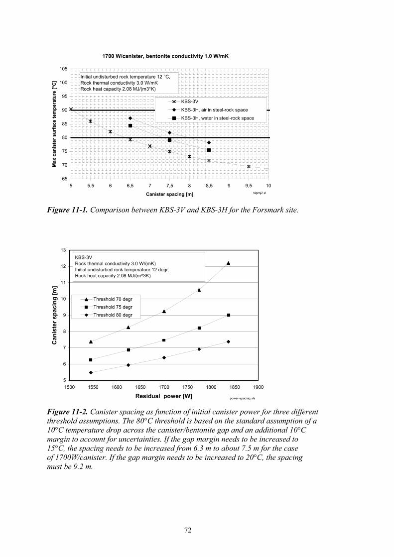
72

1700 W/canister, bentonite conductivity 1.0 W/mK

65

70

75

80

85

90

95

100

105

5 5,5 6 6,5 7 7,5 8 8,5 9 9,5 10


Max

can

iste

r s

urf

ace

tem

per

atu

re [

°C]

KBS-3V

KBS-3H, air in steel-rock space

KBS-3H, water in steel-rock space

Initial undisturbed rock temperature 12 °C,Rock thermal conductivity 3.0 W/mKRock heat capacity 2.08 MJ/(m3*K)

t4proj2.xl

Figure 11-1. Comparison between KBS-3V and KBS-3H for the Forsmark site.

5

6

7

8

9

10

11

12

13

1500 1550 1600 1650 1700 1750 1800 1850 1900

Residual power [W]

Can

iste

r sp

acin

g [

m]

Threshold 70 degr

Threshold 75 degr

Threshold 80 degr

KBS-3V Rock thermal conductivity 3.0 W/(mK) Initial undisturbed rock temperature 12 degr. Rock heat capacity 2.08 MJ/(m^3K)

power-spacing.xls

Figure 11-2. Canister spacing as function of initial canister power for three different threshold assumptions. The 80°C threshold is based on the standard assumption of a 10°C temperature drop across the canister/bentonite gap and an additional 10°C margin to account for uncertainties. If the gap margin needs to be increased to 15°C, the spacing needs to be increased from 6.3 m to about 7.5 m for the case of 1700W/canister. If the gap margin needs to be increased to 20°C, the spacing must be 9.2 m.

73

12 Discussion and conclusions

12.1 Relevance of the results

12.1.1 Canister position and repository size

All results in this report refer to a canister in the central parts of the repository. For the time-ranges considered here, about 10 or 20 years after deposition, all canisters that are not located in the outermost tunnels can be regarded as being in the central parts. Figure 12-1 illustrates this. The maximum temperatures for a central canister, a corner canister and a canister at the edge of the repository are compared with the temperature of one separate canister.

Figure 12-2 shows that the repository size is of small importance for the maximum temperature. To bring the maximum temperature down by one or two degrees, the size of the repository must be reduced to include less that 200 canisters.

Figure 12-1 and figure 12-2 together show that the maximum temperature results in this report are relevant for a very large majority of the canisters also if the repository should be split in a number of sub-repositories.

KBS-3V; 1837 W/canister; canister spacing 8m rock conductivity 2.8 W/mK; bentonite conductivity 1.1 W/mK

0

10

20

30

40

50

60

70

80

0 10 20 30 40 50 60 70 80

Time [years]

Can

iste

r su

rfac

e te

mp

erat

ure

[°C

]

Central canister

Corner canister

Edge canister

One single canister

h175.xl

Figure 12-1. Canister surface temperatures for a number of assumptions regarding the canister position within the repository area.

74

0

10

20

30

40

50

60

0,1 1 10 100 1000 10000

Time [years]

Tem

per

atu

re i

ncr

ease

[°C

]

Infinite4000 canisters, Base Caseone halfone 9thone 25th

Figure 12-2. Central canister. Rock wall temperature increase for a number of repository size assumptions. From /Hökmark and Claesson, 2001/. The canister power is 1545 W. The canister spacing is 6 m and the tunnel spacing 40 m.

12.1.2 Deposition sequence

All results presented here were obtained assuming all canisters to be deposited simultaneously. The analytical solution derived by /Claesson and Probert, 1996/ has been used to examine the significance of this assumption /Hökmark and Claesson, 2001/. In that study, the deposition was made in steps, each step including 3 tunnels and with 5 years between the steps. No difference was found compared to simultaneous deposition of all canisters. Figure 12-3 shows results obtained by use of the analytical solution described in Chapter 3. Temperatures at the canister surface are shown for two cases: simultaneous deposition of all canisters and deposition tunnel by tunnel with 2 years between tunnels. Canisters within the individual tunnels were deposited simultaneously. The maximum difference, 0.2°C, is found after 4 years, while the difference at the time of temperature maximum is much less. If the canisters had been deposited individually in the calculation, for instance one canister a weak, there would be differences soon after deposition, but not on a year time-scale.

12.1.3 Tunnel spacing

The reference tunnel spacing is 40 m. This value has been used throughout in this report. Figure 12-4 shows the contribution from other tunnels than the local one for different tunnel spacing assumptions. The maximum canister surface temperature will be reached some 10 or 20 years after deposition. Reducing the tunnel spacing from 40 m to 25 m, for instance, would mean an increase of that temperature by between 8°C and 12°C for the 1700 W/canister case. Figure 12-5 shows a direct comparison for a case with a power of 1837 W/canister. The maximum canister temperature will increase by about 11°C if the tunnel spacing is reduced from 40 m to 25 m.

75

70

72

74

76

78

80

82

0 10 20 30 40 50 60 70 80 90

Time [years]

Can

iste

r su

rfac

e te

mp

erat

ure

[°C

]

Deposition tunnel by tunnel with 2 years between tunnels

Simultaneous deposition of all canisters

KBS-3V, 1837 W/canisterSpacing 8 mRock heat conductivity 2.8 W/mKInital temp 15 degrRock heat capacity 2.08 MJ/m^3KBentonite conductivity 1.1 W/mK

sequencetest.xls

Figure 12-3. Deposition distributed over time compared with simultaneous deposition of all canisters. For an individual canister, the difference is of no importance.

Contribution from other tunnels

0

5

10

15

20

25

30

35

40

45

50

0 20 40 60 80 100

Time [years]

Te

mp

era

ture

inc

reas

e [

°C]

20253035404550

Canister power 1700 WCanister spacing 7 m,Rock conductivity 3.0 W/mK,Rock heat capacity 2.08 MJ/m^3K

Contribution from other tunnels

0

5

10

15

20

25

30

20 25 30 35 40 45 50

Tunnel spacing [m]

Tem

pae

rtu

re i

ncr

ease

[°C

]

10 years

20 years

Canister power 1700 W,Rock heat conductivity 3 W/mKRock heat capacity 2.08 MJ/m^3KCanister spacing 7 m

tunspace.xls

Figure 12-4. Temperature contribution from other tunnels than the local one.

76

0

10

20

30

40

50

60

70

80

90

100

0 10 20 30 40 50 60 70 80 90

Time [years]

Can

iste

r su

rfac

e t

em

pe

ratu

re [

°C]

40 m 25 m

KBS-3V, 1837 W/canisterSpacing 8 mRock heat conductivity 2.8 W/mKInital temp 15 degrRock heat capacity 2.08 MJ/m^3KBentonite conductivity 1.1 W/mK

sequencetest.xl

Figure 12-5. Maximum canister temperature for two tunnel spacing assumptions.

12.2 Model uncertainties

12.2.1 Non-uniform slots

For KBS-3H, the canister is not centred in tunnel. The effects of this could not be captured by the axially symmetric analytical and numerical models. Comparisons made between a perfectly centred model and a model in which the canister rests on the bentonite and the bentonite on the steel cylinder gave a difference of 2°C at maximum. This value is an upper bound estimate, obtained from plane 2-D models that will exaggerate the difference. Disregarding effects of the geometry not being centric may mean an error of about 1°C and is conservative.

12.2.2 Convection

All calculations were conducted without regard to any possible effects of convection in air-filled slots. This approach has been used in all previous analyses and is justified by the small slot widths /Bjurström, 1997/. In the KBS-3H concept, the two inner slots have even smaller widths (5 mm) than the one considered in the KBS-3V concept (10 mm). Disregarding convection for the outer 42.5 mm slot is conservative, but the possible effects of convection on the results are difficult to estimate. The effects should be small because the air-filled outer slot does not mean more than about 3.5°C of temperature excess even without convection effects, as found from Figure 6-2 by comparing the b- and c-cases.

12.2.3 Radiation

The main source of uncertainty is the temperature offset at the canister/bentonite interface.

77

For KBS-3H, that offset will be about 7.5°C if the slot air-filled, as found from Figure 6-2 by comparing the b- and e-cases. This offset is sensitive to the assumptions made regarding the copper surface heat emissivity. The value used here, e = 0.3, is more conservative than the value e = 0.63 used in previous studies /Ageskog and Hansson, 1999/ and was obtained by back-calculation of experimental results from the Prototype repository in Äspö HRL. Theoretically, if the canister surface emissivity is that of polished copper, the gap effective conductivity would be about 0.03 W/(mK) (cf Figure 4-3) instead of 0.045 W/(mK), and the temperature offset would amount to 11°C.

For KBS-3V, similar estimates can be made. The canister-bentonite temperature offset may be about 17°C if the preliminary results of the recently installed canisters in the Prototype repository /Goudarzi and Börgesson, 2004/ are translated to 1700 W/canister and reduced by 10% to account for the power reduction between deposition and the time of maximum temperature.

12.2.4 Bentonite thermal conductivity

Effects of over-predicting the bentonite thermal conductivity are small, perhaps about 2°C. This was demonstrated for KBS-3V in Chapter 5 (cf Figure 5-4). In addition, Figure 3-6 shows that a significant desaturation would be required to bring the bentonite thermal conductivity below 0.9 W/(mK).

12.2.5 Rock heat capacity

Effects of over-predicting the rock heat capacity are very small, perhaps about 1°C (cf Figure 5-3).

12.2.6 Rock thermal conductivity

In all analyses presented here, heat transfer in the rock has been assumed to take place by linear heat conduction in a homogeneous medium. In reality, there may be some non-linearity and some convection. In the KBS-3V concept, the backfilled tunnel will give some inhomogeneity.

The nomographic charts (cf Chapters 5 and 8) show that it takes an error of about 0.5 W/(mK) to give an error of 5°C in maximum canister surface temperature. Below, effects of non-linearities and effects of the backfilled tunnel are shown to be much smaller. Effects of spatial variations in host rock properties may be more important, but are not included here. In principle it would however be possible to use combinations of analytical and numerical methods to investigate effects of typical variations on different scales.

Convection and non-linearity Due to the low porosity and low permeability of crystalline rocks, effects of convection can be disregarded /Thunvik and Braester, 1980/.

78

The conductivity of most crystalline rocks is reduced by 10% to 15% when heated from 20°C to 100°C /Kukkonen and Lindberg, 1995/. Sundberg suggested a 0.1% reduction per °C /Sundberg, 1991/. At the time of temperature maximum, the rock temperature increase is about 50°C at the hottest rock point (cf Figure 3-2) and much less few decimeters away. Ten meters above the plane of the canisters, the increase is about 20°C after 20 years (cf Figure 9-2). As an estimate, the average effective rock conductivity may have been reduced by 3% at the time of maximum temperature, i.e. by about 0.1 W/(mK).

These observations support the assumption made here and in most work dealing with the thermal evolution of the repository host rock, i.e. that heat transfer in crystalline rocks is largely a question of linear heat conduction.

Effects of the back-filled tunnel in KBS-3V Figure 12-6 shows the KBS-3V near-field on different scales. They light-grey areas indicate nearfield rock volumes. The backfill conductivity is set at 1.5 W/(mK) and the rock conductivity at 2.8 W/(mK). The nearfield volume fraction occupied by the tunnel is about 4% in the left part of the figure and 2.5% in the right part. The arithmetic and geometric near-field conductivity is 2.75 W/(mK) and 2.73 W/(mK), respectively, counting the volume shown in the left part of the figure as being involved in the heat transfer. For the volume shown to the right, corresponding estimates are 2.77 W/(mK) and 2.76 W/(mK), respectively.

The two examples are simplistic but show that the effects of the backfilled tunnel are small as far as possible influences on the effective rock thermal conductivity are concerned. The effect corresponds to about 0.05 W/(mK).

Figure 12-6. Nearfield volumes used for effective rock conductivity estimates.

79

12.3 Margins and thresholds

12.3.1 Data uncertainty margin

Material data uncertainties do not differ much between KBS-3V and KBS-3H. Effects of errors in bentonite thermal conductivity values, rock heat capacity values and rock thermal conductivity values do not seem to add up to the 10°C margin. As far as these parameters are concerned, the 10°C margin is well on the conservative side.

The ranges of possible errors in canister power and in the initial undisturbed rock temperature are difficult to estimate. In principle, it should be possible to assume that there will be no error of any significance in the determination of these parameters.

12.3.2 Gap margin

The 80°C threshold has been used throughout here. For the KBS-3H concept, the 10°C gap margin covers the effects of the two inner 5 mm gaps well (cf Chapter 6, section 6.3.4), assuming the copper emissivity to be 0.3. For the KBS-3V concept, the inner gap may give a larger offset using the same copper emissivity value (cf Table 4-1). Figure 12-7 shows results presented in previous chapters, but now compared with other thresholds.

For KBS-3H, there are two thresholds: one for the case of an air-filled steel/rock space (b-case) and one for water-filled steel/rock space (c-case). The c-case threshold has been moved up by 3.5°C. This corresponds to the effects of the gap between bentonite and steel, which cannot remain open if there is water in the steel/rock space. For KBS-3V, the threshold has been moved down by 5°C to account for a 15°C offset across the canister/bentonite gap.

1837 W/canister, rock conductivity = 2.8 W/(mK)

KBS-3V

KBS-3H, water in steel/rock space

KBS-3H, air insteel/rock space

70

75

80

85

90

95

100

6 6,5 7 7,5 8 8,5 9 9,5 10 10,5 11 11,5 12 12,5 13


Ma

x c

ans

iter

su

rfac

e t

emp

erat

ure

[°C

]




Analytic_2.xls

Initial rock temperature 15 degrRock heat capacity 2.08 MJ/(m^3K)Bentonite conductivity 1.0 W/(mK)

Figure 12-7. Intersections of spacing/temperature curves with modified thresholds.

80

12.4 Conclusions

The nomographic charts presented here are based on verified calculation schemes and allow, in principle, for direct determination of the canister spacing required to meet the design temperature criterion. The schemes allow for fast and efficient analyses, such that a dense coverage of cases can be obtained.

An important feature of the nomographic charts is that the slopes of the spacing/ temperature curves vary systematically in the range between about 0.2 m/°C and about 0.7m/°C.

The determination of margins is a key issue. For systems that give high temperatures (low conductivity rocks) with gentle slopes of the spacing/temperature curves close to the threshold intersection, smaller margins would bring the required spacing down significantly.

The major uncertainty in the use of the nomographic charts is the application of proper gap margins. The temperature offset between canister surface and bentonite, in particular, is difficult to predict. For KBS-3H, the 10°C margin seems to be sufficient. For KBS-3V, this is not necessarily the case. The calculated temperature offsets for KBS-3H turned out to be smaller than the estimated ones, whereas results from field experiments suggest that this will not be the case for KBS-3V.

If it were possible to treat the canisters such that the copper surface emissivity can be raised to 0.6 or higher, then the 10°C margin would be sufficient also for the KBS-3V concept. Similarly, if it were possible to refine the emplacement technique, such that the initial clearance between canister and bentonite blocks could be reduced from 10 mm to 5 mm, the 10°C would be sufficient.

The nomographic charts are well adapted for examining the importance of different site specific conditions and of canister power for a given concept. Comparison between concepts requires additional assumptions, for instance regarding the gaps. If the outer KBS-3H gap can be assumed to be water-filled and the KBS-3V canister/bentonite gap must be assumed to be 15°C, then the KBS-3H concept will require less total tunnel length than KBS-3V.

The initial power is important. Raising the power from 1545 W/canister to 1837 W/canister means that the spacing must be increased by about 5 m for a high-temperature case (KBS-3H, b-case, 2.8 W/(mK)). For a low-temperature case (KBS-3V, 3.2 W/(mK)) the extra spacing would be 1.6 m.

The initial temperature is important independently of concept comparisons. Here, the initial undisturbed rock temperature was set at 15°C as reference. An initial temperature of 12°C (as in the Forsmark site application) would be equivalent to moving all thresholds up by 3°C, meaning spacing savings of between 0.6 m and 2 m.

81

References

Ageskog L, Jansson P, 1999. Heat propagation in and around the deep repository. Thermal calculations applied to three hypothetical sites: Aberg, Beberg and Ceberg. SKB TR-99-02. Svensk Kärnbränslehantering AB.

Bird R B, Stewart E W, Lightfoot E N, 2002. Transport Phenomena. John Wiley and sons, NY.

Bjurström H, 1997. Värmeöverföring i en spalt. SKB AR D-97-07. Svensk Kärnbränslehantering AB.

Börgesson L, Fredriksson A, Johannesson L-E, 1994. Heat conductivity of buffer materials. SKB TR-94-29. Svensk Kärnbränslehantering AB.

Cheremisinoff N P, 1986. Fundamentals of Momentum and Heat Transfer. In: Handbook of Heat and Mass Transfer, Vol 1: Heat Transfer Options. Gulf Publishing Company, Houston, Texas.

CIMNE, 2000. CODE_BRIGHT. A 3-D program for thermo-hydro-mechanical analysis in geological media. Departamento de Ingeneria del Terreno; Cartigrafica y Geofisica, UPC, Barcelona.

Claesson J, 1996. Partial differential equations – technical applications. Depts.of Mathematical Physics and Building Physics, Lund University of Technology, Lund.

Claesson J, Probert T, 1996. Temperature field due to time-dependent heart sources in a large rectangular grid. SKB TR-96-12. Svensk Kärnbränslehantering AB.

CRC, 1973. Handbook of Chemistry and Physics. The Chemical Rubber CO, Cleveland, Ohio.

Gaffner D, 1983. Strålning. In Bygghandboken. Liber, Stockholm.

Goudarzi R, Börgesson L, 2003. Prototype Repository. Sensors data report, Report nr: 6. SKB IPR-03-30. Svensk Kärnbränslehantering AB.

Goudarzi R, Börgesson L, 2004. Prototype Repository. Sensors data report, Report nr: 8. Svensk Kärnbränslehantering AB. In preparation.

Hottel C H, 1954. Chapter 3 in Heat transmission, 3rd ed, McGraw-Hill, NY.

Hökmark H, Claesson J, 2001. Use of an analytical solution for calculating temperatures in repository host rock. Proceedings of the 6th international workshop on key issues in waste isolation research. Accepted for Engineering Geology.

Ikonen K, 2003. Thermal analyses of a KBS-3H type repository. Posiva 2003-11, Posiva, Helsinki.

Kukkonen I, Lindberg A, 1995. Thermal conductivity of rocks at the TVO investigation sites Olkiluoto, Romuvara and Kievetty. Report YJT-95-08, Nuclear Waste Commission of Finnish Power Companies, Helsinki.

82

Sundberg J, 1991. Thermal properties of the rocks at Äspö Island. SKB HRL Progress Report 25-91-09

SKB, 1999. Deep repository for spent nuclear fuel. SR 97 Post-closure safety, Main Report Volume I. SKB TR-99-06, Svensk Kärnbränslehantering AB.

Thunvik R, Braester C, 1980. Hydrothermal conditions around a radioactive waste repository. SKBF/KBS TR 80-19, Svensk Kärnbränslehantering AB.

ISSN 1404-0344CM Digitaltryck AB, Bromma, 2004

Documents

Thermal dimensioning of the deep repository