THERMAL CONVECTION IN THE INTERIOR OF THE EARTH

1935 Dec. Thermal Convection in the Interior of the Earth 343

thing in this case. There are alternative possible identifications of S from Strasbourg to Kew, covering the doubtful region. Stonyhurst and Edin- burgh show a small but sharp movement that may be sP.

The very large movement after S on 1926 June 26 appeared at first to be the surface waves, but it is not of the usual type. The indirect S at Uccle is recognized by the entry of a longer period, with little change of amplitude ; the movement identified as S, is very large on the horizontal components. This merges into the train, the period becoming longer instead of shorter as in the early stages of the surface waves of normal earthquakes. It ends abruptly at 17m 188 without the previous rise to a large amplitude that we expect for a minimum group-velocity, and is followed by a much smaller coda.

1929 February I shows small surface waves. It happens that most of the records also show the Atlantic earthquake of Feburary 2, which was one of those used by Bullen and me. It also has rather small surface waves, and Fr. Rowland mentioned to me that he had suspected deep focus for it also. In this case, however, the P residuals do not show focal depth, nor is S early up to 60°, so that the depth seems to be normal.

Uccle on 1926 June 26 shows a very small early P , with a larger P after it, the later giving an insignificant residual. On previous occasions I have interpreted such a phenomenon as due to a small primitive P followed by a larger sP, but this explanation is not available here because the primitive P movement is certainly large. There is evidence, however, of a weak motion a few seconds ahead of the main P, whatever its interpretation may be.

THERMAL CONVECTION I N THE INTERIOR OF THE EARTH

Chaim L. Pekeris, D S c . (Communicated by Dr. Harold Jeffreys)

(Received 1935 December 12)

Abstract.-The paper deals with thermal convection in the shell of the earth, caused by various assumed zonal temperature perturbations. One temperature perturbation here treated is that due to the difference in the temperature distribution under a continental crust made up of 10 km. of granite on top of 20 km. of basaltic material and a sub-oceanic crust consisting of 25 km. of basalt. The kinematic viscosity v was assumed to be 3 x 1021, as estimated recently by N. A. Haskell from a study of the uplift of Fennoscandia after the ice load. It is found that when g , Y , p and a, the coefficient of volume expansion, are constant, the velocities and their gradients are proportional to the amplitude of the temperature perturbation and to (uglv), while the stresses are independent of the viscosity. The velocities are found to be of the order of I cm./year. The shearing stress exerted by the convective substratum on the crust is of the order of 10' dyn./cm.2, while the normal stresses are about 10 times larger. The

Dow

nloaded from https://academ

ic.oup.com/gsm

nras/article/3/8/343/642312 by guest on 30 Decem

ber 2021

344 Dr. Chaim L. Pekeris, 3, 8

crust is pushed upwards under the warmer (continental) regions and pulled downwards under colder (oceanic) regions. The maximum stress-difference occurs at the bottom of the crust over the centre of the oceans or continents. The surface inequalities are nearly compensated.

I. Introduction.-Thermal convection presents a problem in hydrodynamics coupled with a problem in heat conduction. Being, usually, of a turbulent character, it has defied, along with nearly all other problems in turbulent flow of real fluids, all attempts at a theoretical interpretation. In fact, it would prove an embarrassing task at present to teach the Stokes of 1851 the theory of turbulent flow. The essential difficulty arises from the non-linear character of the forces due to the convective transport of momen- tum. When, however, the motion is slow, the convective forces become negligibly small in comparison with the viscous forces, and the problem is then manageable. Such a case arises in the initial laminar convection in an horizontal layer of fluid heated from below, as in the experiments of BCnard, Low and Brunt and Sir G. Walker and his students.* It appears from the theoretical investigations of Lord Rayleigh and Jeffreys t that when the temperature is uniform over the upper and lower horizontal boundaries, there exists a critical vertical temperature gradient below which any convection will be damped out by viscosity. This gradient /3 depends on the properties of the material and the thickness h of the layer in the following manner :--I

A=- g 4 h 4 kv ’

where X is a non-dimensional constant of the order of a thousand, g-the constant of gravity, a-the coefficient of volume expansion, k-the coefficient of thermometric conductivity and v-the kinematic viscosity. Difficulties due to convection arise in all measurements of thermal conductivity of liquids and gases.§ There, convection is usually minimized by either narrowing

* H. Bknard, Rwuegenerule des Sciences, xii, 1261, 1309 (1900) ; Ann. d. Chemie et de Physique, xxii, 62, 1901. A. R. Low and D. Brunt, Nature, 115, 299, 1925. G. Walker, Science Progress, 29, 385, 1935.

t Rayleigh, Phil. Mug., 32, 529, 1916 ; H. Jeffreys, ibid., 2, 833, 1926 ; Proc. Roy. SOC., 118, 195, 1926 ; Proc. Cumb. Phil. SOC., 26, 170, 1930.

1 Jeffreys uses approximate methods for the determination of 1. In the case of two conducting rigid boundaries and an assumed dependence of the velocities on x and y of the form sin Ix . sin my I find that 1 is a solution of the following equation :-

sin hu sin hu, sin hu3 u1 u2 US .L( I - cos hu, cos hug) = ei*13- ( I - cos hul cos hua) + e- - x ( I - cos hug cos hu,),

where

and UI =(a2 - a)*, i l g = ( U S + ei43S)8, u3 = (a2 + e 4 ~ / ~ 6 ) 4 ,

ua =h2(la +ma), da = A d .

For u = 3 , 6=25.15 and 1=1768, in satisfactory agreement with Jeffreys’s value of 1726.

Q P. W. Bridgman, The Physics of High Pressure, p. 309, 1931 ; H. S. Gregory, Proc. Roy. SOC., 149, 35, 1935.

Dow


ic.oup.com/gsm


ber 2021


the space occupied by the fluid or, in the case of gases, by rarefaction. Even then there is still some residual convection and it is in this connection that the theory of slow thermal convection was initiated in 1879 by A. Oberbeck.* He studied the convection arising in a gas which is contained between two concentric spheres, the inner sphere being maintained at a higher temperature than the outer. Such an apparatus was used by Kundt and Warburg for measurements of thermal conductivity. He found that when the coefficient of volume expansion and the temperature gradient are small (slow convection), the laminar convection takes place in meridional planes, as shown in the accompanying figure.t

Furthermore, convection will exist, in diminishing amounts, under any temperature gradient, however small. The reason for the non-existence of a

FIG I .-Stream lines in a fluid contained between concentric spheres, the inner having the higher temperature. (After Oberbeck.)

critical temperature gradient is clearly the non-coincidence of the direction of the temperature gradient with the direction of gravity. Similar results would be obtained in the case of a horizontal layer of fluid heated from below if the temperature on either the upper or lower surface is made horizontally non-uniform. The pattern of flow would correspond to the

* A. Oberbeck, Ann. d. Physik, 7 , 271, 1879. This reference I obtained from a paper on the same subject by R. W. Babcock, Phys. Rev., 35, 1008, 1930.

Oberbeck integrates his equations stepwise. A simpler procedure is as follows :-

Let u = -, v =z then it follows that, if the divergence of the velocity is zero,

w = _- -- It can then easily be shown that vef =o, of which the appropriate

solution is f = -! +A + Alr + A2rz + Asis +A4+. The A's can then be determined to

fit the boundary conditions. In a later paper (Ann. d. Physik, 11,489,1880), Ober- beck introduces the function f, but he does not arrive at vef =o.

t In Oberbeck's work and in the present discussion it is assumed that the density of the convective fluid depends on the temperature but not on the pressure. The latter effect can approximately be taken care of by using the potential instead of the actual temperature. It is to be noted that the horizontal gradients of the actual and the potential temperatures are nearly equal.

a?f axaz ayaz9

ay a 2 f

a x 2 ay2. A r

Dow


ic.oup.com/gsm


ber 2021


pattern of the perturbing temperature : the liquid would rise over regions which are maintained above the mean temperature of the surface and it would sink over the relatively colder regions. On the other hand, a fluid entrapped between a gravitating hot sphere and a colder crust will not flow when the temperature gradient is below a certain critical value, provided the direction of the temperature gradient coincides with the direction of gravity.* However, when a zonal temperature perturbation is maintained at the bottom of the crust, it will be shown later that convection will be initiated even though originally the density in the fluid increases with depth.

2. On the Possibility of Thermal Convection in the Interior of the Earth.- In the following we shall discuss the possibility of thermal convection in the range of depths of a few tens of kilometres (the crust) to 2900 km. (the boundary of the core). This problem has been discussed extensively by geophysicists and geologists,-/- but it appears that the only thing upon which they can be said to agree at present is the desirability of making a quantitative study of it. For thermal convection to exist two circumstances are essential : there must be a temperature perturbation which is not com- pletely destroyed by the ensuing circulation and the material must not have any great strength. As for the temperature perturbation, one usually thinks of the temperature gradient which has persisted since solidification at depths greater than a few hundred kilometres and which is due to the increase of melting-point with pressure.1 Jeffreys finds that in a layer 2500 km. thick and with a temperature gradient of IO C. per km. the viscosity required to stop convection is of order I O ~ ~ , a value above the current estimates of the viscosity of the shell. A more effective thermal perturbation is the zonal variation of the temperature in the substratum caused by the non-uniform heating of the crust. The circulation generated by it is ultimately reinforced by any radial superadiabatic temperature gradient which existed originally, so that by this approach to the problem we are actually not neglecting spontaneous convection. The mean temperature of the ground decreases in continental regions from the equator to pole by about 60°.11 This surface temperature variation, being independent of the time, penetrates to great depths. Another source of differential heating is that due to the lack or

* This fact has been pointed out by F. A. V. Meinesz, K . Akad. Amst. Proc., 37, 37, 1934 ; Gravity Expeditions at Sea, 2, 53, 1934. When a critical temperature gradient exists, the differential equations determining the velocities are homogeneous ; in the other case the equations are non-homogeneous, the right-hand side containing the term of the original temperature distribution whose gradient does not coincide with the direction of gravity.

t A. Holmes, Wash. Acad. Sci. Joum., 23, 169, 1933, and the literature cited there ; R. A. Daly, Igneous Racks and the Depths of the Earth, p. 226, 1933 ; Jeffreys, Geogr. Journ., 78, 451, 1931 ; Earthquakes and Mountains, p. 168, 1935 ; F. A. V. Meinesz, loc. cit.

1 L. H. Adams, Journ. Wash. Acad. Sci., 14, 459, 1924; Jeffreys, The Earth, p. 138 ; M.N.R.A.S., Geophys. Suppl., 3, 6, 1932.

5 The Earth, p. 140 ; M.N.R.A.S., Geophys. Suppl., 3, 60, 1932. 1 ) W. Koppen, Die Klimate der Erde, p. 42,1923. The temperature in the oceans

below 2 km. is uniformly around 2' C. Some latitudinal temperature gradient must have existed within the earth even before solidification.

Dow


ic.oup.com/gsm


ber 2021


thinness of the granitic layer over oceans. Taking the mean depth of the Pacific to be 5 km. below the mean continental level and assuming the crust under the Pacific to consist of 25 km. of basalt as against the continental crust made up of 10 km. of granite on top of 20 km. of basalt, I computed the temperature distribution in the substratum.* On comparing this with the temperature distribution computed by Jeffreys for the continental substratum, I find that at the bottom of the crust the temperature difference is about 200° C., and that it decreases with depth d in the substratum in the exponential form e-0*0046d, where d is measured in kilometres. This exponential is represented by curve Ia in fig. 2. It should be remarked here that only the order of magnitude of the quantities involved is significant for the following discussion.

As for the strength of the asthenosphere, opinions differ widely. Holmes, Daly and others think that for periods of the geological time-scale the per- manent strength of the asthenosphere is nil. On the other hand, Jeffreys infers from the anomalies of gravity that the strength of the asthenosphere is between 4 x 10' to xoS dynes/cm.2. Further support for this view he finds in the excessive distortion of the figure of the mo0n.t Admitting this, let us estimate the minimum temperature perturbation necessary to overcome this strength. Consider a sphere in the substratum of a radius R equal to 1000 km., and let it be maintained at a temperature T above its surroundings. The non-hydrostatic force is approximately (ugp T x volume)

* Jeffreys has shown (Gerl. Beitr. z. Geoph., 18, I , 1927) that if a layer of thickness H generating heat at a rate A cal./c.c./sec. bounds an infinite half-space of the same thermal conductivity k and if the initial T =S +mx and it is kept zero at x =o, the temperature distribution at a later time t is given by

Using Jeffreys's value of 0.004 for k for basalt and his value of 0.36 x 1 0 - l ~ for A, we have

(AH2/zk) =(0.36 x 10-'~)(6~25 x 1ol2)/(2 x 0.004) = 2 8 1 O C. Now, since the temperature of the ocean bottom is at least as low as the mean surface temperature of the continents, we should write (x -5 ) for x , if we wish to compare our results with Jeffreys's equation (34) on p. 1 5 3 of The Earth. Hence, with

m=3O/km., S=14ooo, T = 1 3 8 5 + 3 x - 1 1 2 0 I -Erf - ( (:;:>I* It must be remarked that the age of the earth of 1.6 x 10' years adopted by Jeffreys should now be increased to at least 2 x 10' years, but this modification will not appreciably alter the results, since the cooling depends on dL More serious are his values of radioactive heat generation, which are now believed to be too high. Thus, from Urry's summary (Proc. Amer. Acad. Arts and Sn'., 68, 142) I find that the heat generation per C.C. per sec. in basaltic and granitic material is 0.11 and 0.52 in units of 1 0 - l ~ cal., as against Jeffreys's values (quoted from Holmes) of 0.36 and 1.3. Prof. R. Evans informs me that his latest values are 0.13 and 0.61. Although the rates of heat generation in granite and basalt are in a higher ratio with the last two authors than with Jeffreys, the smaller absolute values will diminish the above computed temperature contrast between sub-continental and sub-oceanic regions, but will not change its order of magnitude.

t The Earth, p. 227.

Dow


ic.oup.com/gsm


ber 2021

348 Dr. Chaim L. Pekeris, 3 , 8

’(2 x 10-5 x 103 x 3.3T x volume) =o.o7T x volume. The shear stress at the surface is then about (0.07T volume/area) E 0.07TR =7 x 108T dynes/cm.2. Clearly a temperature contrast of a few tens of degrees is sufficient to overcome the above-mentioned strength of the asthenosphere and to start horizontal flow.* One could perhaps also argue that convection will be initiated in a medium of finite strength if the potential stresses which will arise from the velocity gradients will be above the strength. We shall see later that this requirement is approximately met in all the cases considered. While it would appear from the above discussion that convection currents in the shell of the earth are not an impossibility, it is not our purpose here to attempt to establish their existence. We shall in the following assume that the shell is a plastic fluid possessing a finite coefficient of viscosity, and shall investigate the nature of the circulation which is caused by a given zonal temperature perturbation in it. We shall first find the distribution of velocities and stresses within the shell by assuming that the crust is rigid and that the core cannot sustain any shearing stress. Next we shall find the distortion of the crust due to the reaction of the convective substratum on it and to the thermal expansion caused by the assumed temperature perturbation. We shall also compute the gravity anomalies at the new geoid level.

3 . The Theory of Laminar Thermal Convection.-Let us adopt a system of polar co-ordinates with the origin at the centre of the earth and a polar axis which does not necessarily coincide with the axis of rotation. We shall assume for simplicity that the initial temperature does not depend on the azimuthal angle (longitude), so that it is a function of r and 8 only. We also neglect the ellipticity of the earth. The motion will then take place, except for a negligible effect of the deflecting force of the earth’s rotation, in meridional planes and the velocity vector will have only two components, the radial u and the zonal v. If we neglect quadratic terms in the velocities, the equations of steady motion are : t

* The matter will flow in the direction of the smaller stress. Jeffreys (M.N.R.A.S., Geophys. Suppl., 3, 59, 1932) concludes that, according to his earlier estimates of the amount of cooling in the crust, the degree of distortion in the cooled region is about 25 times greater than in rocks when on the verge of crushing. He therefore concludes that the material will yield and flow horizontally.

t A. B. Basset, Hydrodynamics, 11, 243. The problem was originally solved in the case R(r) constant, in Cartesian co-ordinates. The components of velocity can then be written as

and f is found to satisfy the differential equation vOf =F(r, z) where F depends on the given temperature perturbation.

Dow


ic.oup.com/gsm


ber 2021


where s stands for the divergence of the velocity. The density will be assumed to vary as p =R(r)(I - aT), where a is the coefficient of volume expansion, assumed constant, T the temperature and R(r) is a non- increasing function of r, representing the effect of pressure on the mean density distribution. From the equation of continuity we have

The temperature satisfies the equation (on neglecting the effect of pressure variation on the density)

P denoting the rate of heat generation by radioactive materials. The time variation has been included in order to allow for the cooling since solidification, an epoch which is greater than the epoch during which a steady convective circulation is established. Let T = To(r, 8, t) + aTl(r, e) + a2T2 + . . ., To being, obviously, a solution of (4) when a =o, hence when no convection exists :

m

paT0/at = k v T 0 + P, T, = t) + 2 Tn(r, t)p,(cos e). 1

Further, for the relatively short time intervals to be considered we may neglect the time-variation of the T ’ S . With Oberbeck, we assume

u = a241 + a%, + . . ., v = av1 + a2v2 + . . . :. s =as,+ a%,+. . . Also, let

m m a m

v1 = C$,(r)-P,(cos O), p , = Cn,(r)P,(cos e), and s1 = Ca,(r)P,(cos 1 ae 1 1

Remembering that - I - a (sin 6%) = - n(n + I)P,, we have sin 8 a0

a, = ( I/rz)d/dr(r2+,) - n(n + I)$,/r,

A + (+I+, - (I/r)n(n + I)$, + (@@A = 0.

and from the a term in (3)

We now substitute in ( 2 ) and, using the identity

we obtain an expression for p , in terms of the velocities :

( 5 )

Dow


ic.oup.com/gsm


ber 2021

3 50 DY. Chaim L. Pekeris, 3, 8

At this point we introduce the assumption that p =constant * and substitute (6) in ( I ) , obtaining after some cancellations the differential equation

=gR(T)Tn, (7)

which together with ( 5 ) determines $, and 4,. mined from the velocities :

The stresses are then deter-

and similarly for P + + ~ . The stresses p , and p,, are identically zero. Equations (7) and ( 5 ) lead to a non-homogeneous differential equation of the fourth order for either +,, or $,. The complementary function of the solution of this equation consists of four simple powers of Y multiplied by arbitrary constants, which can be determined to fit the boundary conditions at the two spherical boundaries. At a rigid surface (the crust) u and w must vanish, while at the boundary of the core u and p , vanish. Finally, T,, the perturbation in temperature caused by the convection, clearly satisfies the equation pc(uz+:%) = kV2 TI.

Again, to be exact, one should include in (8) the thermal effects of changes in pressure.

We shall now discuss the solutions of the above system of equations for a few given types of temperature perturbations (T,), as described in Table I.

(a) R(r) =po =constant, v =p/po =constant.

By ( 5 ) 4 , + ( 2 / ~ ) + ~ = ( ~ / r ) n ( n + I)$ , , with which we eliminate $, from (7), obtaining

[~/n(n + I ) ] ( Y ~ & + 8r6, + 124,) - 24, - (4/r)& - ( 2 / ~ ~ ) + ~ + (1/r2)n(n + I ) + ,

For n = I this equation becomes

while for n = 2 it is

= (g /+n. (9)

( 1 0 )

( 1 0 ’ )

Yi& + SY& + 841 - (8/~)$1 =2(g/Y)T1,

y2&. + 8 ~ 4 2 - (24/y)d2 + (24/y2)W2 = 6(g /v )~*

= Iooe-kb+kr[I - ( I / ~ Y ) ] / [ I - ( ~ / k b ) ] . E = Iooe-kb(g/v) . [I - (1/M)]- l .

* A variable p, especially when in the form of a power of r, could be handled in the following analysis. t See entries in Table I.

Dow


ic.oup.com/gsm


ber 2021

351 1935 Dec. Thermal Convection in the Interior of the Earth

c-3 c-1 2Eekr(k2 k +'> 2rS 2r k6 21 2r2 2r3 ' $ 1 = + 1 + K 4 1 ) = --+-+c++c2r2+- (12)

r4

6 ~ - 3 zEe",( k4 k3 3k2 6k 6 [ r 4 - 7 - 6c2r+- k6 --+-+--- 2 21 2r2 13 +-)I. r4 ('4) p,, = p cos e - -

If in the above formulae we use 1000 km. for the unit of length (so that b, for example, has the numerical value of 6-34), then the c's have the following values :- C-3 = 175148F) C-1 = - 9778.26F) c =2817*96F, C , = - 348156F, where F = Ioog . {vkSb3[1 - ( 1/kb)]}-', uF having a dimension of a velocity. If we evaluate F in c.g.s. units and use 1000 km. as a length unit in (11) and ( 1 2 ) and multiply by a, the velocities will be obtained in cm./sec., while the stresses obtained from (13) and (14) will be in units of 10-8 dynes/cm.2.

II. T~ = 100(b3/rS)(t6 - d) . ( 6 5 - d) -1 . E = 100b3(g/v) . (b6 -

c-3 c-1 a61nr a5

21.9 2r $~=- -+++c++c~Y~+E

12rS 7a6 aslnr)], - 6c2r + E - - - -+ - ( 35 6r2 r2 /

c - ~ = - 25.9107E, c - ~ = - 241910E, C =77.56973, c2 = - 0.9041zqE,

where, as before, the unit of length is 1000 km. The velocities being proportional to aEr4, we have to multiply the values obtained from ( I S ) and (16) by u x 10l6 to obtain velocities in c.g.s. units, while the values from (17) and (18) have to be multiplied by a x IO~. This applies also to all the following cases.

111. 72 = 133.3(b3/r3)(r6 -a6) . (b6 -a6)-'. E _= 133 .3b3(g/v) . (b6 -a6)-'.

Dow


ic.oup.com/gsm


ber 2021

352 Dr. Chaim L. Pekeris,

c-4 =93*5988E, c - ~ = 168.409E, c1 =9.896643, c3 = - 0449201E. Equations (IS), (20), (21) and (22), with different values for b and a, apply also to cases V and VI. The corresponding constants have the following values :-

V. c - ~ = - 6846.843, c-, = 2948.65E, c1 = 23.78743, c3 = - 0.566629E. VI. C-4 = - 7749*54E, C-2 =3010-27E, c1 =23*4917E, c3 = - 0.563096E. (b) R(r) =po(b2/r2).

ds =(I/r)n(n+ I)$~, v =vo(r2/b2)

[I/.(. + 1)](r2& + 6r& + ws) - 2& - (2/r)&+ ( I/r2)n(n + I)& =(gbz/vor2)T,. (23) When n =2, (23) becomes

riT2 + 6r& - 642 - ( 12/r)d2 + (36/r2)+, = 6(gb2/uor2)~2. (24) IV. T~ = 133.3(bs/r3)(r6 - as) . (b6 - u6)-l. E = 133.3b3(g/v) . (b6 - a5)-l,

c-3 c-, ra 42 = + - + c2r2 + c3r3 + 6Eb21nr

$ -1 + - - 3 - 2 + 1 + - c- c- c r2 ~ ~ 7 . 3 + Eb21nr( - - r2 - c ) + E b 2 ( -$+$), p,,=psin28 2r4 r3 ( 5 ,or.) (4:+2)]

2 - & 2 2r3 3r2 2 , I0 109

2c2r - 3c3r2 + Eb%r 32 - 9a6 + Eb2 9 gC-3 3c-2

10c-3 z~c - , cgr2 - Eb21nr(z) - Eb2( + 31, p,, =t9.[ - - - - - 1"' 3r3

c - ~ = 1989.56, c - ~ = - 2507.14, c, = 12.8253, c3 = 1.58896. The stream lines, which in this case of steady motion are also trajectories,

are found from the equations :

dr rde -- dr rde u v ' G- ap;

dt=-=-

*sw Let R(r) = constant, n = I, $1 = +rdl +

:. r2+* = A/cos 8 sin2 8.

The A's are constant along a stream line, but differ from one stream line to another. Knowing that the stream lines are normal to the radius vector

Dow


ic.oup.com/gsm


ber 2021


at 0 =90° and 6 = 5 4 7 O for n = I and n = 2 respectively, one can easily trace a group of stream lines, once the functions and r242 are computed for various values of r. Finally, the absolute value of the difference of the principal stresses I SP I is given by [(Pee - PrJ2 + (2Pre)2]*. At the upper surface of the shell (r =b) Pe, =P,, so that I SP I = I 2P,@ I . At 0 =o, I SP, I is given by the following expressions in the respective cases :-

4. The Elastic and Thermal Distortion of the Crust. Gravity Anomalies.- In the preceding section the upper boundary of the convective shell was assumed to be spherical. Actually the crust becomes slightly distorted from its original spherical shape on account of the normal and tangential stresses which are exerted at its inner surface as well as on account of the thermal expansion caused by the original temperature perturbation. To be exact we should have applied the boundary conditions for the flow at the new surface, but since this surface differs from the spherical by only a few km. at the most, and since it is seen from Table I1 that the change of the velocities and stresses within such a distance is small, it is evident that the flow will not be appreciably altered. We can thus treat the problems of the flow in the shell and of the distortion of the crust independently. The general nature of the distortion of the crust can be seen at once. Over the rising current it will be pushed upwards and it will be pulled downwards over the sinking currents. Since the thickness of the crust is small in comparison with the radius of the earth, the rise will be such that the weight of the matter of the shell which is introduced above the original surface over a rising current nearly equals the applied normal force. The actual rise will be slightly less on account of the horizontal drag, which is, however, relatively small, as seen from Table 11. The radial pressure and azimuthal tension form a favourable arrangement for large stress-differences, which, it will be shown, are at a maximum at the bottom of the crust and over the centre of the rising or sinking currents. The thermal expansion superimposes a radial extension of the crust which is about three times the linear extension that would result from the given temperature perturbation. The rise of the outer surface is thus slightly increased, while the rise of the lower surface is diminished. The introduction of lateral compression tends to diminish the original stress-differences.

The equations of equilibrium of an homogeneous elastic medium subject to thermal stresses and to forces applied at the boundaries are : *

where A is the divergence of the displacement, a the coefficient of volume expansion, and T the perturbation in the temperature. These equations can be solved by putting

~~ ~

* Jeffreys, M.N.R.A.S., Geoph. Suppl., 3, 59, 1932.

Dow


ic.oup.com/gsm


ber 2021

3 54 Dr. Chaim L. Pekm's, 31 8

with

and (A + 2p)V24 = (A + $p)aT,

aAl (A + p)- + pv2wi = 0. ax,

It is found that because of the special type of the forces applied at the

, the appropriate solution of (28) can

be built up from the types * nA + (3n + 1)p

(n + 3 P + (n + 5)P' (u, w, w ) = r(? a ")-, + a,(x, y, x)wn, a, = - 2 .ax' ay' ax

where w, and 4, are spherical solid harmonics of degree n. If we use polar co-ordinates and denote by u and w the radial and zonal ( 8 ) components of the displacement, we have for a solution of (25)

Here A, B, C, D are arbitrary constants and

(33) A(n+1)+p(3n+2) A(n - 2) +p(n - 4) ' f in= -2

which is obtained from the expression for a, by putting (-n - I) for n. Under the assumption A=p, which is nearly true for the material of the crust, the expressions for the stresses are

2D + 2C(n - I)rn-2 -

* Love, Elasticity, p. 250, 1934.

Dow


ic.oup.com/gsm


ber 2021

1935 Dec.

~ = ~ + - . - + - - - a ~ = - - a ~ + - - + - - + 2 av 2~ 5 1 0 2 a24 2 a 4

P r a e r 3 9 r2 ae2 r ar

Thermal Convection in the Interior of the Earth 355

+%{ 2Arn +++ 2B 2Crn-2 + + a,(5 + n)] + a e 2

The absolute value of the difference of principal stresses [ 6P I is given by

The boundary conditions are : I 6P I = [(Pee - P,,)' + (2P,e)2]1'2. (37)

a t r = b Prr = -gpu, Pro =o, (38) at r = b + H PTT, =Fo +&o - P ~ O , Preo = Go. (39) Here b is the inner radius of the crust, Fo and Go the values of the normal and zonal stresses due to the convection ; the quantities without subscripts refer to the outer surface of the crust, while the quantities with the subscript zero refer to the inner surface. It should be noted that P,, and Fare positive for tensional stresses.

Referring now to equation (27), we see that if T is of the form T(r)P,, a solution for 4 can be found which is of the form F(r) - P,. The variation of u and P , with 0 will then be similar to that of the temperature perturbation.

v and Pro vary as -, while Pee has, except for the case n = I , a composite

variation. It is clear that equations (38) and (39) form four independent equations for the determination of the constants A , B, C and D, even in the case n = I .

The anomalies in gravity are due to two effects working in opposite directions. Considering the subcontinental region, we have a positive contribution to gravity* due to the rise of the upper surface of the crust and, to a smaller degree, due to the rise of the boundaries between the crust and shell and between the shell and core, at each of which there is an increase in density. There is also a negative contribution to gravity on account of the lower density of the subcontinental matter caused by the assumed temperature perturbati0n.t Let the boundaries of the crust and of the core be represented by

r=c+uP, , r o = b + u Z 2 , rl=a+u,P2, c = b + H , (40) where the subscript I refers to the boundary of the core. Then the perturbation of the potential outside the earth is

crust is zero.

at geoid level vanishes since it is given by

t The elastic dilatation causes a change in density p' given by - pA', where p is the density of the crust and A' is defined by (26) and is given by the second term in (32). Since p' is nearly constant within the crust, the resulting gravity anomaly, which in our examples is negative, is given by o.6g(Hp'/pc)P2.

ap, ae

* The gravity anomaly due to a first order harmonic in the distortion of the The external potential @ being of the form A/P, the gravity anomaly

a 2 ( - a7, - ; b e

Dow


ic.oup.com/gsm


ber 2021

356 Dr. Chaim L. Pekeris,

Y =-b 4*f uc4 + (po - p)b4uo + (p l - po)a4ul]Pz. 5r3

Within the crust the above expression for the potential is to be modified

by changing the term -pu-P, 4*f c4 into 4rf -pu-Pz. r2 The gradient of the potential 5 y3 5 c - -

thus changes on crossing the outer boundary by 4rfpuP2, which is the appropriate boundary condition. If the density is assumed to be of the form p =R(r)(I - aT), with

T = To(r) + T(r)P,, then the perturbation of the potential 0 due to the thermal expansion satisfies the equation

In case I11 of the preceding section, R(r) = p o =constant 3-3 ; V2@ =4rfR(r)a~(r)P,. (43)

within the shell and is zero within the core. We shall assume the same form for T(r) within the crust, since at a depth of about 5 km., where the temperature of the ocean bottom is uniformly about 2 O C., the subcontinental temperature is, with an assumed geothermal gradient of about 30' C. per km., around 150' C. We shall also use the same value of 3.3 for p , and shall later apply a correction to take account of the smaller density of the crust (2.7). A solution of (43), valid within the shell and crust is

@ = (44)

where B and C are arbitrary constants. Within the core the solution is

4rfAr2P,, while outside the earth it is 4mfD. - On imposing the conditions r3

of the continuity of the potential and its derivative at the boundary of the core and at the surface of the earth, we obtain four equations for the solution of the four unknown constants. In particular

c2 a5 a7 B = c= --. I 0 15C3' ' 4

The perturbation of gravity at geoid level, which is obtained from

is given then by

where p denotes mean density of the earth.

Dow


ic.oup.com/gsm


ber 2021


equation

Its solution is

The perturbation of gravity at geoid level is now given by

the term in brackets being due to the distortion of the crust. The above are the appropriate gravity anomalies for a crust of density 3-3. Since the actual density is about 2.7, we have to add the attraction of a layer of matter of density p’ = 4 3 . 3 - 2.7)TP2 and of the thickness of the crust. The correction is given by o.6g(Hp’/pc)P2 which, with T = 1 3 3 - 3 , amounts to 0.8mgal for a thickness of 30 km. and is proportionately greater for a thicker crust.

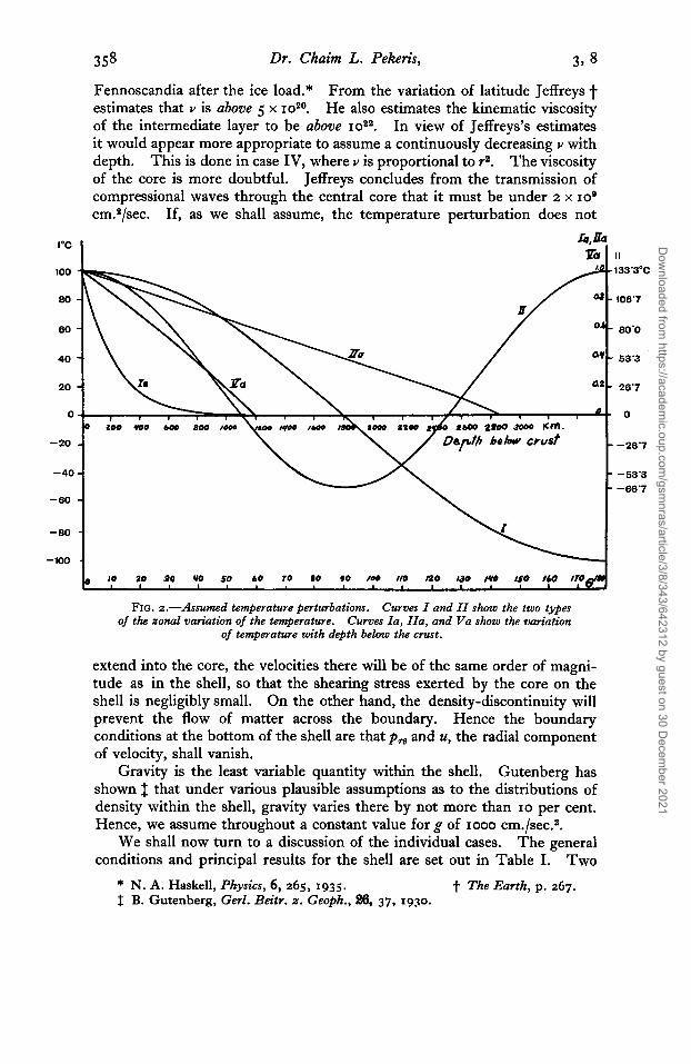
5. Some Cases of Thermal Convection in the Earth.-We shall now discuss six cases of thermal flow in the earth, so chosen as to exhibit the effect of variations in the type of temperature perturbation, the distribution of density and viscosity and the thickness of the convective region. Before doing this we shall recall some of the assumptions introduced in the calculations and some general results of the preceding theoretical discussion. We have assumed the density within the shell to be given by p =R(r)(I - aT) , where R(r) is either a constant or increases with depth as (1/r2). The latter assumption rather exaggerates the increase of mean density with depth on account of compression. a was assumed constant; the assumed expression for T consists of a term depending only on the radius and a zonal perturbation of the form T(r)P,, 2(cos 0). We have also assumed constant values for g and for the coefficient of viscosity p. Further, we have neglected terms in a2 in the velocities and stresses, as well as the effect of the deflecting force of the earth‘s rotation. The last two assumptions can be shown to be valid for the extremely slow circulation in the shell. It is found that under the above assumptions the velocities are proportional to (TUg/V) where v denotes the kinematic viscosity-the ordinary viscosity divided by the density. The values of the velocities are thus quite sensitive to the adopted value for v. The stresses, on the other hand, being proportional to p and to the gradients of the velocity are independent of v. Hence more weight is to be attached to our results concerning the magnitude of stresses within shell and crust, the distortion of the crust and the gravity anomalies, than upon the numerical values of the velocities. We have adopted a value of 3 x 1021 cm.2/sec. for v, as recently estimated by N. A. Haskell from a study of the uplift of

Dow


ic.oup.com/gsm


ber 2021


Fennoscandia after the ice load.* From the variation of latitude Jeffreys t estimates that v is above 5 x 1020. He also estimates the kinematic viscosity of the intermediate layer to be above 1 0 ~ ~ . In view of Jeffreys's estimates it would appear more appropriate to assume a continuously decreasing v with depth. The viscosity of the core is more doubtful. Jeffreys concludes from the transmission of compressional waves through the central core that it must be under z x 1o9 cm.2/sec. If, as we shall assume, the temperature perturbation does not

This is done in case IV, where v is proportional to r2.

k J a Pi I II

100

80

80

40

20

0

-20

-40 - - -53'3 - -88'7

-80 -

-80 - -100 .

10 zo aa yo so bo T O 80 90 lob ti0 iao 130 two ISO 160 I T O ~ 1 1 1 I I , I 1 I ,

FIG. 2.-Assumed temperature perturbations. Curves I and 11 show the two types Curves l a , IIa, and V a show the variation of the zonal variation of the temperature.

of temperature with depth below the crust.

extend into the core, the velocities there will be of the same order of magnitude as in the shell, so that the shearing stress exerted by the core on the shell is negligibly small. On the other hand, the density-discontinuity will prevent the flow of matter across the boundary. Hence the boundary conditions at the bottom of the shell are that p , and u, the radial component of velocity, shall vanish.

Gutenberg has shown 1 that under various plausible assumptions as to the distributions of density within the shell, gravity varies there by not more than 10 per cent. Hence, we assume throughout a constant value for g of 1000 cm./sec.z.

The general conditions and principal results for the shell are set out in Table I. Two

Gravity is the least variable quantity within the shell.

We shall now turn to a discussion of the individual cases.

* N. A. Haskell, Physics, 6, 265, 1935. 1 B. Gutenberg, Gerl. Beitr. z. Geoph., 26, 37, 1930.

t The Earth, p. 267.

Dow


ic.oup.com/gsm


ber 2021


types of zonal temperature variation are assumed, one varying like cos 0, the other like P, (cos 8) =(3)(3 COS, 8 - I). These are shown respectively by curves I and I1 in fig. 2. If we care to think of warmer regions as subcontinental and of colder regions as sub-oceanic, then the distribution of

t FIG. 3.--Stream lines in a convective shell under a crust made up of a hemispherical

The assumed temperature perturbation corre- The velocities are indicated, to scale, by the

The crust is 30 km. thick and is

continent and a hemispherical ocean. sponds to curves I and l a in fig. I. arrows at the places whne they are radial and zonal.

drawn to scale.

continents and oceans in the above two types will be as indicated in figs. 3 and 4 respectively.* The ratio of the amplitude of the temperature perturbation in the interior to its value at the surface is shown by curves Ia, IIa and Va, for cases I , I1 to IV, and V and VI respectively. The stream

Clearly the * The ocean of fig. 3 can be considered as representing the Pacific. axis of the figure does not have to coincide with the axis of rotation.

Dow


ic.oup.com/gsm


ber 2021


lines in figs. 3 and 4 were drawn for cases I and I11 respectively, but these two types of circulation are characteristic for the cos 0 and P,(cos 0) distributions of temperature. The detailed distribution of velocities and stresses is shown in Table 11. These are seen to have their smallest values in case I,

FIG. +--Stream lines under a crust ma& up of two polar continents and an equatorial The temperature perturbation corresponds to curves 11 and IIa of fig. I . The ocean.

thickness of the crust is 20 km. and is drawn to scale.

where the temperature perturbation penetrates least into the interior. Cases V and VI are next in order of magnitude. Together, they show the effect of a density discontinuity at 1200 km. depth. Since the lower half of the shell will be dragged into convection by the thermally perturbed upper half, its effect on the latter will be intermediate between that of rigid and free boundary-the conditions of V and VI respectively. In case I11 we see the effect of greater penetration of the temperature perturbation into the

Dow


ic.oup.com/gsm


ber 2021


interior, such as would apply for the latitudinal temperature variations over continental regions. In comparison, case I1 shows that an attenuation of the zonal variation in the temperature inhibits convection, a result which is rather surprising, since one usually associates the flow of higher harmonic types with greater losses of energy by internal friction. We shall, however, see later that the frictional losses are altogether out of proportion to the existing kinetic energy, so that the above criterion is ineffective, at least for the low harmonics. Case IV shows the effect of a continuously increasing density. The reason for the greater intensity of convection is the fact that with an assumed constant coefficient of ordinary viscosity the kinematic viscosity decreases with depth. Now, as mentioned above, one essential result of the theory is that when a, g, p and v are constant, the velocities and their derivatives are directly proportional to (mglv), where T denotes the amplitude of the temperature perturbation. Since, in IV v decreases at the bottom of the shell to about one-third of its value at the top, we should expect the intensity of convection to be greater than that in I11 by a factor of about 2.

Generally, p,, is greater than pro by a factor of about 10, especially so in the upper half of the convective region. The sign of p,, is such that warmer (continental) regions of the crust are pushed upwards by the convective substratum, while colder regions (oceanic) are pulled downwards. The corresponding reaction on the core is in the opposite direction. The absolute value of the difference between the principal stresses I6P 1 varies with 8 and r. At the upper surface of the shell it equals I2P,e I . The radial distribution of I 6P I at 8 =o is shown in Table I1 by the columns marked lap,, I in cases I, I11 and IV. These stress differences are of the order of magnitude of the strength which Jeffreys imputed to the asthenosphere. The tangential stresses pTe are about 104 times greater than the shearing stress due to the equatorial attraction *-the largest of the forces hitherto suggested for the supposed drift of the continents and the wandering of the poles.

The results for the distortion of the crust and the gravity anomalies are shown in Tables I11 and IV for the Pl and P, types of temperature dis- turbance. It is seen that as we go from the bottom to the top of the crust the displacements and Po, vary least, P,, diminishes slightly, while Pro drops to zero. Doubling the thickness of the crust does not change u and P,, appreciably, while v, Po0 and SP are. reduced by about a half. The maximum stress difference always occurs at the bottom of the crust in the region of maximum amplitude of the temperature perturbation. In the Pl case, P,, and Pee vanish at the equator. SP at the surface vanishes there, while at the bottom of the crust it has the small value of P,,. If failure of the crust is to occur, it is thus more likely to happen at the centre of the continents or the oceans than at their boundaries. This is true, to a less degree, for the P, case.

The gravity anomalies in the P, case are, with the exception of case IV, positive over continents and negative over oceans. The inequalities are

* The Earth, p. 301.

Dow


ic.oup.com/gsm


ber 2021


nearly compensated,* since the anomalies due to the assumed temperature perturbation in the core are -120P2 and -150P2 for cases I11 and IV respectively. These values should be compared with the fields of positive isostatic anomalies ( + 3omgaZ) observed by Minesz over 0ceans.t The observed values could be brought about by a less penetrating temperature perturbation such as was assumed in case I.

Finally, we shall discuss briefly the energy transformations in the convective shell. If we neglect the work done by the shell in maintaining the circulation in the core, we have ]: for the rate of energy dissipation by internal friction

+ where v is the velocity vector and integration is carried over the volume of the shell. For n = I

+ 1 a u 1 a

r a6 r ar curlv =-----(rv)=sinO

I have computed a few values of curl; for case I1 and I find that they are of the order of 10-16, as was to be expected, since the velocities (10-') change by IOO per cent. in a distance of about IO* cm. and curlv is proportional to the velocity gradients. Hence the rate of energy dissipation per C.C. is

P + about 1oa2 x I O - ~ O = I O - ~ ergslsec. The kinetic energy per C.C. is - v 2: 10-l~ 2

ergs. If the thermal forces should vanish, the energy would therefore decrease to (I/e) of its value in about 10-'I seconds, a result which is not surprising in view of the enormous viscosity of the material.

The major part of this work was done at the Massachusetts Institute of Technology, where I received the advice and encouragement of Professor L. B. Slichter. In the later stages I benefited from the criticisms of Dr. H. Jeffreys.

due to the inequalities. the error is small.

t LOC. cit. $ H. Lamb, Hydrodynamics, 6th ed., p. 581, 1932.

+

It is a pleasure to acknowledge my indebtedness to them.

* In computing the distortion of the crust, we neglected the gravitational forces Since, however, the inequalities are nearly compensated,

Dow


ic.oup.com/gsm


ber 2021

-

-

- 1 I1

[I1 IV V V

I -

Max

i- m

um

Abs

olut

e V

alue

of

Y

Out

er

Rad

iu

b

-

I000

km. -

6-34

6.

34

6.35

6.

34

6.35

6.

35 -

Max

i- m

um

Abs

olut

c V

alue

of

0

Inne

r hd

ius

I000

km* I A

ssum

ed T

empe

ratu

re P

ertu

rbat

ion

O c.

10

' dy

n./c

m.a

TABLE

I

10'

dyn.

/cm

.

R(r

) in

p =

R(Y

) x (I

-an

0.06

14

2.63

9.

47

14.8

0.

142

0.25

3

Bou

ndar

y C

ondi

tions

: V

anis

hing

Qua

ntiti

es

0.16

6 8.

38

14.8

0.53

4 1

-10

19.7

cm./y

ear

cm./y

eai

0.37

7 5.

27

9-87

16

-0

1-55

2

-01

13'9

73

.6

96.4

38.0

42

'9

132

Dow


ic.oup.com/gsm


ber 2021

I000 km.

v/si

n 8

6-35

6.34

6-30

6.20

6-10

5'90

5.70

5.50

5.40

5-30

5.20

5.15

5

.00

480

460

4.40

4.20

4.00

3.80

3.60

3.50

3.47

p+e/

sin 8

u/co

s 8

cm./y

ear

0

0.000283

0.00753

0.0191

0.0312

0.0420

0.0467

0.05

08

0.0543

0.0558

0.0592

0.0614

0.0607

0.0570

0.0502

0.00297

0.0403

0-0274

0.00277

0

0.0116

v/si

n 8

cm ./y

ear

0

0.0429

0.115

0.150

0.162

0.135

0.0938

0.0717

0.0495

0.0169

- 0.0142

- 0.0524

- 0.0861

-0.1

15

-0.138

-0.154

-0.164

-0.166

-0.163

-0.162

0.0277

I

plel

sin

8

lo7

dy

n./c

m.*

- 0.377

-0.167

- 0.0793

0.0482

0.06

08

0.0630

0.0636

0.0632

0.0627

0.0604

0.0561

0.0

5 I

0

0.0449

0.0380

0-0204

0~00890

0.002 I 7

- 0.303

0.0122

0.0299

0

TA

BL

E

I1

I1

107

dyn.

/cm

.a

- '3.9

- 11.6

- 7.26

- 4.52

- 1.67

- 0.511

- 0.0388

0.0788

0. I54

0.203

0.255

0.279

0.292

0.301

0.310

0.318

0.327

0.337

0.342

0.343

0.220

I @o

I

107

dyn.

/cm

.*

0

0.0134

0-0370

0.0415

0.0597

0.0567

0.0481

0.0427

0.0369

0.0307

0.0275

0.0176

0-0107

0.0256

0.0406

0.0556

0.0701

0.0892

0.0908

0.0037

0.0833

u/co

s 8

cm./y

ear

0

0.00417

0.0488

0. I37

0.419

0.799

I '23

1 -45

1-67

1.87

1-97

2.23

2.61

2.63

2.60

2.39

I -98

1.38

0.593

0- I 42

0

cm./y

ear

I dG.71m

.P

0

0.643

2.04

3-15

457

5-08

482

444

3.93

3-30

2.94

1.75

- 0.0565

- 1.98

- 3.88

- 5-61

- 7.03

- 8-00

- 8.38

- 8-30

- 8-24

- 5.27

- 4.91

- 404

- 3.23

- 1.75

- 0.475

0.601

I -06

I -48

1.84

2.43

2-81

3-00

2.99

2.76

2.32

I .65

0.735

0.180

2.01

0

prrl

cos

8

I o7

dyn.

/cm

.a

- 73.6

-71.1

- 64.8

- 58-8

- 47.4

- 36.9

- 27.1

- 22.6

- 18.2

- 14.1

- 12.1

- 6-35

6.75

0.590

12.1

16-7

20.4

23-3

25.1

25.6

25.7

Dow


ic.oup.com/gsm


ber 2021

I

1000 km.

6-35

6.34

6-30

6-20

6.10

5-90

5-70

5-50

5 *40

5.30

5-2

0

5-15

5.

00

480

4.60

4.40

4.20

4.00

3.80

3-60

3.50

3 *47

o/si

n 20

TA

BL

E

II-~

ontd

.

pre/

sin

20

UlP,

cm./y

ear

0

0.0245

0.556

0.210

I .63

3.04

4.61

6-17

7.25

8.16

9.06

9.47

9.3 1

8.5 I

7.03

487

2-09

0.499

0

v/si

n 20

cm./y

ear

0

1.51

408

6-09

8.58

9.33

8.66

6.88

5.0

0

2.78

-

0.5

10

- 3.94

- 7-25

- 12-6

- 14.2

- 14.8

- 14.7

- 14.6

- 10.2

111

@*/

sin

20

I o7

dyn.

/cm

a

- 9.87

- 8.98

- 7.30

- 5.74

- 3.00

- 0.733

1.10

2.5

2

3.33

3.93

4.43

4.60

404

3.33

2-33

1-03

0.2

5 I

4.46

0

PrdP

z

I o7

d yn

./cm

.8

- 96.4

- 84.5

- 76.9

- 62.3

-48.8

- 36.2

- 92.4

- 246

- 16.5

- 8.87

0.51

5 9.02

16.6

23.4

31.9

3343

37.3

38.5

38.8

I 6PO

I

107

dyn.

1cm

.t

0

0.90

2-5

2

3-89

5-94

7-10

7.44

7-01

6.24

5.12

3.12

0.65

5.30

2.2

0

8-49

11.6

I4 3

15.4

15.7

4Pa

cm./y

ear

0

0.0253

0.296

0.831

2-53

4.79

7.32

8.58

9.82

11.0

11.5

13.0

143

14.8

14'4

13.0

10.5

7-03

2-90

0.873

0

IV

dyn.

/cm

.z

I 1°'

cm./y

ear

0 I a98

6.36

9.96

15.0

17.4

17.2

17.0

15.9

I45

13.6

10.6

5.80

0.401

-

5.15

- 10.4

- 14.9

- 18.2

- 19.7

- 19.5

- 19.5

- 16.0

- 15.0

- 12.8

- 10.7

- 6.75

- 3.32

- 0.355

0.952

2.14

3.22

3-71

5.01

6.32

7.12

7.40

7.10

6-17

4'52

2.07

0.512

0

Plrl

P,

107

dyn.

/cm

.a

~

- 13

2 - 129

- 113

- 97.6

- 81.9

- 66.3

- 58.5

- 50.6

- 42.8

- 38.9

- 27.2

- 11.8

- I21 3 4.4

18.2

32.1

44.8

55.6

63.4

65.6

66.1

I spo

I

I o7

dyn.

/cm

.'

0

1.18

3.88

6.21

9-81

12.0

12.9

12.8

12.5

11.8

11.3

9-60

6.68

2.35

2-34

7.38

I 2.4

16-8

20.8

20

. I

21.1

Dow


ic.oup.com/gsm


ber 2021

TA

BL

E

II-c

ontd

.

cm./y

ear

6.35

6.34

6.30

6-20

6.10

5-90

5-70

5.50

5 -40

5'30

5.2

0

5.15

10

7 d

yn./c

m.%

0

0-00360

0.0271

0.0618

0.126

0.142

0.0993

0.0633

0.0279

0.00371

0

0

0.215

0.468

0.529

0.274

- 0.178

- 0.504

- 0.534

- 0.435

-0.187

0

- 1-55

- 1.16

- 0.490

0.0237

0.618

0.684

0.283

- 0.0689

- 0.508

- 1-02

- 1.30

107 d

yn./c

m.*

- 38.0

- 33.7

- 25.7

- 18.2

- 5-

32

486

12.1

14.6

16.3

17.1

17.1

cm./y

ear

0

0.00466

0.0366

0.0866

0. I94

0.253

0.230

0.184

0.0421

0. I20

0

VI

v/si

n 20

cm./y

ear

0

0.284

0.651

0.792

0.586

0.0232

- 0.592

- 0

.840

- 1.01

- 1.1

0 -

1.10

&@

/sin

20

107 d

yn./c

m.8

- 2-01

- 1-57

- 0

.80

2

-0.184

0.641

0.970

0.704

0.460

0.163

0.879

0

107 dy

n./c

m.¶

~

- 42'9

- 38.7

- 30.6

- 23.2

- 10.4

- 0.169

7.16

9.69

11.4

12.3

12.4

Dow


ic.oup.com/gsm


ber 2021

TA

BL

E

111

Ela

stic

Dis

tort

ion

of C

rust

and

Gra

vity

Ano

mal

ies

due

to a

Fir

st O

rder

Zon

al T

empe

ratu

re P

ertu

rbat

ion

6P-.

sg -

107 dy

n./c

m.*

-

89.9

o

50.0

o

Rem

arks

The

rmal

dis

tort

ion

of c

rust

neg

lect

ed.

to7

dyn.

/cm

.*

- 1

1.5

- 1

1.5

107 dy

n./c

m.*

107 dy

n./c

m.*

107 dy

n./c

m.P

107 dy

n./c

m.e

10

7 d

yn./c

m.

- 10

.6

- 0.

377

0

79.3

79

.3

- 1

0.5

- 0.3

77

0

39.5

39

.4

vo

ain 2

8

km.

18.2

8.76

5.60

9.22

20.3

7.65

v --

sin

2t

km.

--

--

18.3

8.87

5.72

9.41

20.4

7.80

107 dy

n./c

m.8

107 dy

n./c

m.=

429P

a +5

74 C

OS

28

230P

a +27

6 co

s 28

r77P

s + 1

76 co

s 28

255P

s +29

1 co

s 28

429p

a +5

75 CO

S 28

229P

a +27

8 co

s 28

163P

, + 17

8 co

s 28

254P

, +29

3 co

s 28

3q

Ps +

638c

osz8

j6.8

Pp +

241

cos

28

322P

s+63

9cos

28

53.6

Pp +

24

2 c

os 2

8

V

S3

-I-1-1- km

. -

2.76

I

'25

km.1 km.

I km. I km

.

-1-I-I-

TA

BL

E

IV

Ela

stic

Dis

tort

ion

of C

rust

and

Gra

vity

Ano

mal

ies

due

to a

Sec

ond

Ord

er Z

onal

Tem

pera

ture

Per

turb

atio

n .

-

-

-

I11

I11

I11 IV

I11

I11 -

I pee

Pe

e, A

e si

n 28

R

emar

ks

km. km.

o7 d

yn./c

m.:

o7 dy

n./c

m.

o7 dy

n./c

m

o7 dy

n./c

m.

o7 dy

n./c

m.

1083

585

434

656

1041

378

2.78

2.77

2.75

3.72

2.76

2.71

2.64

2-61

2.58

3-45

2.66

2.63

- 69.

8

-69.

1

-68.

3

-91.

4

- 70'

3

- 69

.7

- 9.

87

- 9.

87

- 9.

87

- 16.

0

- 94

7

- 9.

87

-80.

1

-80.

1

-80.

1

-110

-80.

1

- 80.

4

The

rmal

di

stor

tion

of c

rust

ne

glec

ted

The

rmal

di

stor

tion

of c

rust

in

clud

ed.

I I

Dow


ic.oup.com/gsm


ber 2021

Documents

THERMAL CONVECTION IN THE INTERIOR OF THE EARTH