THERMAL CHARACTERISTICS AND THE DIFFERENTIAL EMISSION MEASURE DISTRIBUTIONDURING A B8.3 FLARE ON 2009 JULY 4

Arun Kumar Awasthi1, Barbara Sylwester2, Janusz Sylwester2, and Rajmal Jain31 Astronomical Institute, University of Wroclaw, Wroclaw, Poland; arun.awasthi.87@gmail.com, awasthi@astro.uni.wroc.pl

2 Solar Physics Division, Space Research Centre, Polish Academy of Sciences, Wroclaw, Poland3 Kadi Sarva Vishwavidyalaya, Gandhinagar, Gujarat, India

Received 2015 December 18; accepted 2016 April 6; published 2016 May 31

ABSTRACT

We investigate the evolution of the differential emission measure distribution (DEM[T]) in various phases of aB8.3 flare which occurred on 2009 July 04. We analyze the soft X-ray (SXR) emission in the 1.6–8.0 keV range,recorded collectively by the Solar Photometer in X-rays (SphinX; Polish) and the Solar X-ray Spectrometer(Indian) instruments. We conduct a comparative investigation of the best-fit DEM[T] distributions derived byemploying various inversion schemes, namely, single Gaussian, power-law functions and a Withbroe–Sylwester(W–S) maximum likelihood algorithm. In addition, the SXR spectrum in three different energy bands, that is,1.6–5.0 keV (low), 5.0–8.0 keV (high), and 1.6–8.0 keV (combined), is analyzed to determine the dependence ofthe best-fit DEM[T] distribution on the selection of the energy interval. The evolution of the DEM[T] distribution,derived using a W–S algorithm, reveals multi-thermal plasma during the rise to the maximum phase of the flare,and isothermal plasma in the post-maximum phase of the flare. The thermal energy content is estimated byconsidering the flare plasma to be (1) isothermal and (2) multi-thermal in nature. We find that the energy contentduring the flare, estimated using the multi-thermal approach, is in good agreement with that derived using theisothermal assumption, except during the flare maximum. Furthermore, the (multi-) thermal energy estimated whileemploying the low-energy band of the SXR spectrum results in higher values than that derived from the combinedenergy band. On the contrary, the analysis of the high-energy band of the SXR spectrum leads to lower thermalenergy than that estimated from the combined energy band.

Key words: plasmas – radiation mechanisms: thermal – Sun: corona – Sun: flares – Sun: X-rays, gamma rays –techniques: spectroscopic

1. INTRODUCTION

Solar flares are some of the most energetic phenomenaoccurring in the atmosphere of our Sun, typically releasing1027–1032 erg of energy in ∼103 s. This immense energyrelease is understood to be powered by magnetic energy via theprocess of magnetic reconnection (Shibata 1999; Jain et al.2011a; Choudhary et al. 2013; Aschwanden et al. 2014;Dalmasse et al. 2015). A typical M-class solar flare can beobserved across almost the entire electromagnetic spectrum(Benz 2008; Fletcher et al. 2011). Therefore, various energyrelease processes occurring at various heights in the solaratmosphere can be probed by the investigation of the observedmulti-wavelength flare emission.

X-ray emission during solar flares mainly originates from thecorona and upper chromosphere. Moreover, the X-ray emissionrecorded during a flare can serve as the best probe for studyingvarious thermal and non-thermal plasma processes (Li et al.2005; Saint-Hilaire & Benz 2005; Jain et al. 2008; Awasthiet al. 2014). Low-energy X-ray emission (<10 keV), alsoknown as soft X-ray (SXR) emission, is understood to originatein the process of free–free, free-bound, and bound-boundemission due to the collision of charged particles (mostlyelectrons) with a thermal (Maxwell–Boltzmann) distribution.On the other hand, high-energy X-ray emission (hard X-rays) isknown to be produced as a consequence of the thick-targetbremsstrahlung of a non-thermal electron beam with the denseplasma in the chromosphere (Brown 1971; Kulinová et al.2011). Moreover, SXR emission during a flare is understood tobe produced by multi-thermal plasma (Aschwanden 2007; Jainet al. 2011b; Sylwester et al. 2014; Aschwanden et al. 2015b).

The study of the thermal characteristics of the flare plasma isperformed through the inversion of the observed X-ray spectrumby postulating an empirical functional form of the differentialemission measure (EM) distribution (DEM[T]). Although DEM[T] plays a key role in deriving the thermal characteristics, and inturn the energetics of the flare plasma, it is less accurately knowndue to the fact that the inversion of the observed radiation needsto be performed, which is a very ill-posed problem (Craig &Brown 1976). Moreover, several DEM[T] schemes whichpostulate a certain functional dependence of DEM on T, namely,single Gaussian, bi-Gaussian, power-law, etc., have beenproposed (see Aschwanden et al. 2015b for exhaustive list ofschemes). Furthermore, a Withbroe–Sylwester (W–S) maximumlikelihood DEM inversion algorithm has been established bySylwester et al. (1980) where the functional form of DEM[T] isnot defined a priori. In this regard, a comparative survey of theaforementioned DEM schemes in the form of the derivedthermal characteristics of the flare plasma is very necessaryprovided that the application of various inversion schemesresults in similar outcomes. In addition, an inevitable restrictionwhen deriving the complete thermal characteristics of the flareplasma is the availability of observations from differentinstruments in certain specific energy bands. Thermal emissioncan be best studied by measuring the X-ray spectrum in typicallythe 1–12 keV energy band. Observations in this energy bandwith high spectral and temporal cadence are very difficult toachieve from a single instrument due to the huge difference influx during a flare across the energy band.Therefore, we examine the temperature dependence of the

DEM from the analysis of multi-instrument data for a B8.3

The Astrophysical Journal, 823:126 (14pp), 2016 June 1 doi:10.3847/0004-637X/823/2/126© 2016. The American Astronomical Society. All rights reserved.

1

flare which occurred on 2009 July 04. As the flare selected forthe analysis is the only common event between SolarPhotometer in X-rays (SphinX; a Polish instrument) and theSolar X-ray spectrometer (SOXS; an Indian instrument), thecombined data set provides a unique opportunity for exhaustivestudy of the complete thermal characteristics of a small flare.Both of the instruments make use of Si PIN detectors forobserving the solar atmosphere in the X-ray waveband.Section 2 presents the observations used for the present studyalong with the specifications of the respective instruments. InSection 3, we present the study of the DEM[T] distributionderived by employing different inversion schemes and itsdependence on the selection of the energy band of the inputSXR spectrum. In Section 4, the thermal energetics of the flare,estimated from the parameters derived from various schemes,are presented. Section 5 is comprised of the summary andconclusions.

2. OBSERVATIONS

We investigate a B8.3 intensity class flare which occurred on2009 July 04 in active region AR11024. AR11024 appeared onthe disk on 2009 July 3 and rotated off the disk on 2009 July15. More than 500 flares or small brightenings have beenobserved by the SphinX mission for the SXR light curve duringthat time. Figure 1 shows the temporal evolution of the X-rayemission recorded by SphinX during this period.

The SOL2009-07-04T04:37 flare, selected for the presentstudy, is the only event observed by both the SphinX andSOXS missions because SOXS usually observed the Sun inX-rays for only 2–3 hr a day. We analyze the X-ray spectra inthe 1.6–5.0 keV and 5.0–8.0 keV energy bands, recorded fromthe SphinX and SOXS missions, respectively. We brieflydiscuss the data and the respective instruments’ specificationsas follows.

2.1. SphinX Mission

We analyze X-ray spectra in the 1.6–5.0 keV band (hereafterlow-energy band) from the SphinX instrument (Gburek et al.2011, 2013; Sylwester et al. 2012). SphinX, a spectro-photometer designed to observe the solar corona in SXRs,was flown on board the Russian CORONAS-PHOTON satelliteon 2009 January 30. SphinX employed three Si PIN diodedetectors to record X-rays in the energy range ∼1.2–15.0 keV.The temporal and spectral cadence of the SphinX observationsare as good as 6 μs and 0.4 keV, respectively. Detailedinformation regarding the observations, the procedure forcalibration, and the data warehouse may be obtained fromGburek et al. (2013) and from the SphinX instrumenthomepage.4

2.2. SOXS Mission

X-ray spectra in the 5.0–8.0 keV band (hereafter high-energyband) during the flare were obtained by the SOXS instrument(Jain et al. 2005, 2008). SOXS employed two semiconductordevices, namely, a silicon (Si) PIN detector for recording X-rayobservations in the energy range 4–25 keV and a CadmiumZinc Telluride (CZT) detector for that in the energy range4–56 keV. The energy resolution of the Si detector is ∼0.8 keVwhile that for CZT detector is ∼1.7 keV. The temporal cadenceof the observations obtained from both detectors is 3 s duringthe quiet and gradual phase of the flare. However, an on boardautomated algorithm allowed the observations to be recordedwith a 100 ms cadence during the rise to the peak phase of theflare. The data obtained during the entire observing period(2003 May–2011 April) of the SOXS mission and the analysisprocedures are available on the instrument homepage.5 In thepresent study, we employ the observations obtained from the Si

Figure 1. X-ray light curve of the solar corona, dominated by the emission from the single active region AR11024 with the flaring emission on top as seen by SphinX.Flare SOL2009-07-04T04:37, selected for the present study, is shown by an arrow.

4 http://156.17.94.1/sphinx_l1_catalogue/SphinX_cat_main.html5 https://www.prl.res.in/~soxs-data/

2

The Astrophysical Journal, 823:126 (14pp), 2016 June 1 Awasthi et al.

detector because it has better energy resolution and sensitivitycompared to the CZT detector.

The left panel of Figure 2 presents the evolution of the X-rayemission as observed by the SphinX (top row) and SOXS(bottom row) missions during the flare in various energy bandsplotted with different colors. The intensity curves shown inblack and red represent the X-ray emission recorded by SphinXin 1.6–3.0 keV and 3.0–5.0 keV, respectively. Furthermore,X-ray emission in 5.0–7.0 keV and 7.0–8.0 keV, drawn in blueand green, respectively, are obtained from SOXS.

It may be noted from the Figure 2 that SOXS receives higherbackground than that seen by SphinX. On the contrary, acomparison of the count rates recorded by SphinX and SOXSin the 4–6 keV range, that is, the energy band commonlycovered by both instruments, revealed that SOXS observationsare lower by a factor of ∼2.5. This may be attributed to thesystematic difference of the sensitivities between the twoinstruments. Mrozek et al. (2012) reported higher flux in theSphinX 3–8 keV energy band compared to the observationsobtained in the same energy range from the RHESSI mission bya factor varying in the range 2–6 keV. On the other hand, acomparison of the SOXS and RHESSI observations in the6–12 keV energy band was performed by Caspi & Lin (2010)which resulted in the agreement of the spectra obtained from

both instruments within 5%–10%. In this study, we preparedcombined data by applying the previously noted “empiricalnormalization factor” in the records obtained from SOXS. Onthe other hand, we consider the flux recorded by SphinX to bethe true flux because this is the only instrument available toobserve X-ray emission at energies less than 4 keV during theflare. Therefore, the difference in inter-instrument sensitivity,and hence normalization factor, in this energy range cannot beestablished. However, in order to study the effect of thisapproximation, we have also carried out an investigation of theDEM distribution by applying the inverse normalization factorto the SphinX records while retaining the original SOXScounts. We discuss the effect of both of the noted cases on thethermal energy estimates as presented in Section 4.

2.3. Geostationary Operational EnvironmentalSatellite (GOES)

GOES refers to a series of satellites dedicated to observingX-ray emission from the Sun as a star in two wavelength bands,namely, 1.0–8.0Å and 0.5–4.0Å. The right column of Figure 2shows the background subtracted flux in the 1.0–8.0Å and0.5–4.0Å bands plotted in black and red, respectively. We treatthe observations averaged during 04:20–04:25 UT as back-ground. The temperature and EM estimated from the flux-ratio

Figure 2. Left panel: temporal evolution of the X-ray count rate in 1.6–3.0 keV and 3.0–5.0 keV obtained from SphinX (top row) and that in 5.0–7.0 keV and7.0–8.0 keV as recorded by SOXS (bottom row). Right panel: GOES flux in 1.0–8.0 Å and 0.5–4.0 Å (top row), temperature (middle row), and emission measure(bottom row).

3

The Astrophysical Journal, 823:126 (14pp), 2016 June 1 Awasthi et al.

technique adopted for GOES data are also plotted in the middleand bottom rows of the right panel in Figure 2, respectively. Itmay be noted that the temperature is found to vary in the range7–12MK while the EM varies in the range (0.003–0.08)´ -10 cm49 3. We use these T and EM estimates to calculate thethermal energy during the flare (see Section 4).

2.4. Morphology of the Flare in ExtremeUltraviolet (EUV) Emission

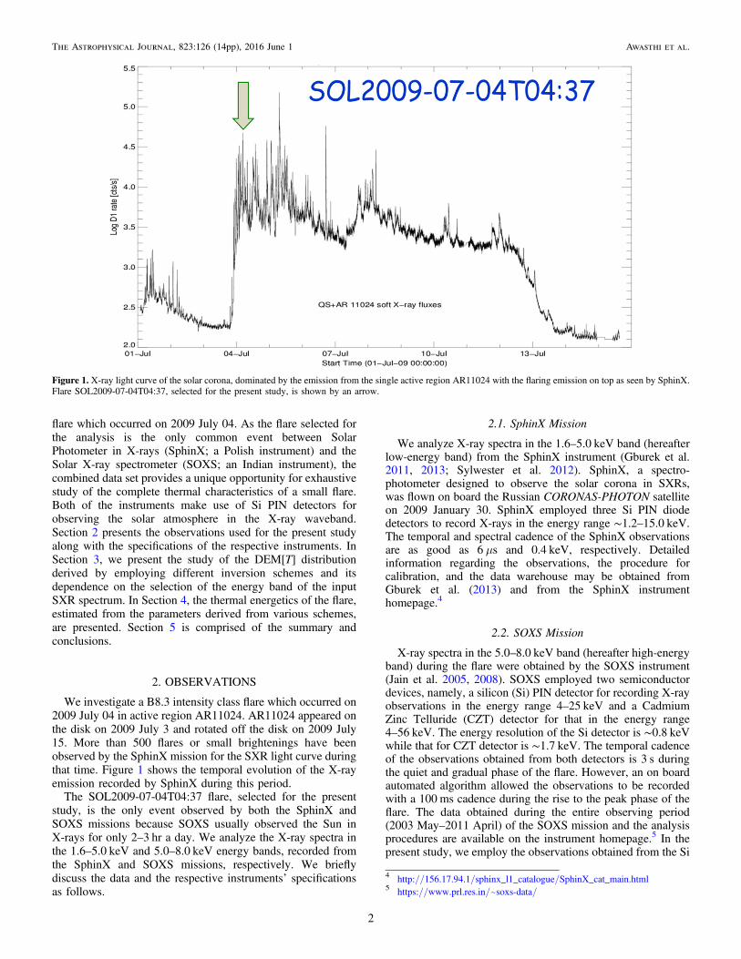
The temporal and morphological evolution of the flaringregion is studied using observations obtained from the EUVImaging Telescope (EIT; Delaboudinière et al. 1995) on boardthe Solar and Heliospheric Observatory (SOHO). Moreover,images in the 171, 284, and 304Å wavelengths, recorded bythe STEREO twin satellites, are also processed. In Figure 3, wepresent the morphological evolution of the flaring region in 171and 304Å during the flare as obtained from STEREO-A and B.

From the time sequence of the EUV images presented inFigure 3, we note that although the flare event considered is asmall B8.3 intensity class flare, it is associated with aneruption. The study of the eruption is outside of the scope ofthis paper. We estimate the volume of the emitting region fromthe EUV images to derive the thermal energetics of the flare aspresented in Section 4.

3. DEM[T] DISTRIBUTION FROM THE APPLICATION OFVARIOUS INVERSION SCHEMES

In order to study the thermal characteristics of the flareplasma, we conduct an exhaustive investigation of theevolution of the DEM[T] relationship employing the X-rayspectra observed from SphinX and SOXS. We explore thedependence of the DEM[T] distribution, which is derived byemploying various inversion schemes to the SXR spectra in

various energy bands, namely, 1.6–5.0 keV (low energy),5.0–8.0 keV (high energy), and 1.6–8.0 keV (hereafter com-bined energy). This study aims to understand the dependenceof the best-fit DEM[T] representing a selective part of the SXRemission, which in turn presents the consequence of therestrictions posed by the co-temporal observations recorded inseparate energy bands from different instruments, namely,SphinX and SOXS. In this study, we employ DEM inversionschemes which postulate the (1) single Gaussian and (2) power-law functional relationship of DEM to T. In addition, we alsoemploy (3) a well-established W–S maximum likelihoodinversion algorithm which is independent of a priori assump-tion of a functional form of DEM[T]. In the following, wepresent the thermal characteristics of X-ray emission during theflare as derived by applying the inversion schemes notedabove.

3.1. DEM Varying as a Single-Gaussian Functionover Temperature

We investigate the best-fit DEM[T] distributions, which wereobtained by employing the scheme of single Gaussianfunctional dependence of DEM on T, on the observed SXRspectrum in the low-, high-, and combined-energy bands.However, first, we also employ this DEM scheme to asynthesized model multi-thermal spectrum. Below, we discussthe two previously mentioned cases.

3.1.1. DEM[T] Distribution of a SynthesizedModel Multi-thermal Spectrum

We synthesize multi-thermal photon spectra using the modelphoton flux arrays corresponding to the isothermal plasma inthe temperature range 1–23MK with a temperature bin of

Tlog = 0.1 MK. The isothermal photon spectrum at specific

Figure 3. Time sequences of images in 171 Å (top row) and 304 Å (bottom row) obtained by the STEREO twin satellites during the flare. The images in the first twocolumns correspond to the side view of the flare obtained from STEREO-A, while those in the other two columns present the line-of-sight view of the flare as seen fromSTEREO-B.

4

The Astrophysical Journal, 823:126 (14pp), 2016 June 1 Awasthi et al.

temperature and EM is calculated using the isothermal model(f_vth.pro) available in the SPectral EXecutive package withinSolar Soft Ware. We derive EM values corresponding to atemperature from the EM model of Dere & Cook (1979), whichis also available in the CHIANTI atomic database (Landi et al.2012; Del Zanna et al. 2015). In addition, we consider theabundance to be 0.1 times the coronal abundance available inthe CHIANTI distribution. Next, the multi-thermal photonspectrum is derived by the weighted sum of the isothermalspectra in following manner:

å==

F w F T EM, . 1k T

T

k k kMT

min

max

( ) ( )

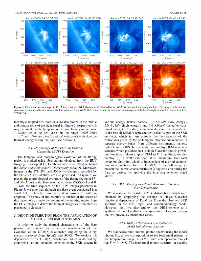
Here, F T EM,k k( ) is the isothermal photon flux and is shown bythe gray (dotted) plots in Figure 4, while the multi-thermal flux(FMT) synthesized in this manner is over-plotted in red.Furthermore, wk is the weight factor which is assumed to be anormalized Gaussian function of temperature with maximum atT = 5.6 MK and FWHM of ∼5MK, as shown in panel (d) ofFigure 5. Such integration allows for a more realistic scheme ofsynthesizing the theoretical multi-thermal spectra compared tothat adopted in Aschwanden (2007) and Jain et al. (2011b).They use a direct sum of the isothermal fluxes with equalweight, in which the synthesized multi-thermal photonspectrum is dominated by the contribution from the isothermalspectrum corresponding to the peak temperature.

Next, we forward fit the synthesized multi-thermal spectrumusing DEM varying as a single Gaussian function of T. Theform of the DEM[T] is considered as

⎛⎝⎜

⎞⎠⎟s

µ- -

TT T

DEM explog log

2, 2

p2

2[ ]

( )( )

where Tp is the temperature at the peak of DEM [T] while σ isthe Gaussian width. By iteratively varying the independentvariables of Equation (2), namely, Tp, σ, etc., a photon fluxbest-fit to the input synthesized multi-thermal photon spectra isderived. It is to be noted that the minimum and maximumtemperature values for deriving the DEM[T] are fixed to

0.087 keV (1MK) and 8.5 keV (100MK), respectively. Thebest fit is assessed by estimating the reduced c2 in each step ofthe iteration, which converges to a small value. Following thisprocedure, we derive the best-fit parameters for the synthesizedmulti-thermal photon spectrum in the low- and high-energybands. Next, we apply a similar procedure to derive the best-fitparameters for the input photon spectrum in the combinedenergy band. Panels (a), (b), and (c) of Figure 5 show thesynthesized input multi-thermal photon spectrum (gray) over-laid by the best-fit model flux drawn in black, blue, and red forthe low-, high-, and combined-energy bands, respectively. Inaddition, normalized residuals are also plotted in the respectivepanels. Moreover, panel (d) presents the DEM evolutioncorresponding to the best-fit model photon spectra.Based on the aforementioned analysis presented in Figure 5,

we find that the best-fit flux derived for the input photonspectrum in the low-energy band (panel (a)) does not provide agood fit (overestimation) to the higher-energy part of thespectrum. On the other hand, the best-fit flux obtained for thehigh-energy band (panel (b)) does not completely follow(underestimates) the low-energy part of the spectrum. Thistrend is clearly represented by the normalized residuals, plottedin the respective panels. Panel (d) of Figure 5 shows DEM[T]for the best-fit model photon flux estimated for the input photonspectrum corresponding to the low-, high-, and combined-energy ranges. This enabled us to perform a comparative studyof the DEM[T] dependence on the input energy bandsselection. We note that the best-fit DEM[T] curves for thelow- and high-energy bands yield high peak values of DEM(DEMp) = 1.72 × 1049 - -cm MK3 1; however, at lowtemperatures, Tp = 7.8 MK for the former (low-energy band)case and relatively lower DEMp = 1.66 × 1049 - -cm MK3 1 athigher Tp = 8.2MK for the latter case. Moreover, moderateDEMp at Tp best fits the input spectra of the combinedenergy band.

3.1.2. DEM[T] Distribution Derived from ObservedX-Ray Emission During the Flare

We analyze X-ray emission in the low-energy (1.6–5.0 keV)and high-energy (5.0–8.0 keV) bands obtained from SphinXand SOXS, respectively, during the flare. In this regard, weprepare a time series of the spectra by integrating the observedX-ray emission into 120 s time intervals during the periods04:27–04:33 UT and 04:38–05:00 UT, which correspond to therise and decay phases of the flare, respectively. On the otherhand, better count statistics during the period 04:33–04:38 UT,which correspond to the impulsive phase of the flare, enabledus to integrate the observation in 60 s time intervals. The timesequence of the spectra obtained in such a way serves as theinput to the inversion scheme.We forward fit the observed SXR spectrum in the low-,

high-, and combined-energy bands using a model photon fluxwhich is derived using the inversion scheme employing asingle Gaussian functional dependence of the DEM on T (seeEquation (2)). Panel (a) of Figure 6 presents the observed countrate in the low-energy band (black color) during the period04:36–04:37 UT, which corresponds to the maximum of theimpulsive phase of the flare. Similarly, the X-ray emission inhigh-energy band (blue color) is analyzed, as shown in panel(b) of the Figure 6, for the aforementioned time interval. Panel(c) presents the analysis of the combined energy band data

Figure 4. Spectra plotted in gray (dotted) represent the isothermal photon fluxcorresponding to the temperature range 1–23 MK with an interval of log T =0.1 MK. The plot drawn in red represents the integrated (multi-thermal)photon flux.

5

The Astrophysical Journal, 823:126 (14pp), 2016 June 1 Awasthi et al.

(from SphinX and SOXS) for the time intervals in a mannersimilar to panels (a) and (b). Best-fit model count rates areover-plotted in red in the respective panels and the derivedvalues are also shown. Panel (d) presents the DEM[T]distribution corresponding to the best-fit model obtained forSXR spectra of the different energy bands.

From Figure 6, it may be noted that the DEMp estimatedfrom spectral fitting of the low-, high-, and combined-energyband data are 1.40, 0.15, and 0.38 (́ - -10 cm MK49 3 1),respectively. On the other hand, Tp is estimated to be 6.37,8.93, and 7.57MK, respectively. It may be noted that the trendof the best-fit parameters, namely, DEMp and Tp, for threecases of input energy bands is in good agreement with thatrevealed by the study of model multi-thermal spectrumemploying the same inversion scheme as presented in theprevious section.

3.2. DEM Varying as a Power-law Function of T

We derive the DEM[T] distribution for the X-ray spectracorresponding to various energy bands, similar to the analysisin the previous section, however, with a different functionaldependence of DEM on T. In this multi-thermal model, DEM isapproximated to be varying with T in the form of a power law

and can be expressed as

⎜ ⎟⎛⎝

⎞⎠µg

TT

DEM2

. 3( ) ( )

Next, employing this DEM scheme, we forward fit theobserved flare X-ray spectrum in the low-energy band obtainedfrom SphinX (black color) as shown in panel (a) of Figure 7.During the iterative procedure for obtaining the best-fit model,the low-temperature value is fixed to 0.5 keV (5.8 MK), whilethe maximum temperature is determined as one of the outputs.All of the spectra during the various time intervals of the flareare analyzed, however, here we present only the results fromthe observations during 04:36–04:37 UT, which are the sameas those presented in the previous section. X-ray emission inthe high-energy band obtained from SOXS (blue color) ispresented in panel (b) of Figure 7. Next, we also fit theobserved X-ray spectrum in the combined energy band asshown in panel (c). The best-fit models are over-plotted by redlines in the respective plots. The parameters of the best fit,namely, Tmax, DEM (at T = 2 keV), and the power-law index(γ), are also shown in the respective plots. Panel (d) shows thederived DEM[T] curves corresponding to the best-fit modelsobtained for different energy ranges.

Figure 5. Panels (a), (b), and (c) correspond to the model photon spectrum (gray) overlaid by best-fit model flux for the 1.6–5.0 keV, 5.0–8.0 keV, and 1.6–8.0 keVenergy bands, respectively. Normalized residuals are also plotted in the bottom row of all the respective panels. The disagreement of the best-fit curves for the higherand lower parts of the spectrum may be noted. Panel (d) presents the DEM[T] corresponding to the best-fit photon flux for all three energy bands. The normalizedweight (wk), employed in Equation (1), is also shown as a gray plot. The dotted lines in panels (a) and (b) at 5.0 keV represent the boundary of the energy rangeconsidered for the spectral fit.

6

The Astrophysical Journal, 823:126 (14pp), 2016 June 1 Awasthi et al.

In Figure 7, it may be noted that at the peak of the impulsivephase of the flare, the Tmax estimated from the observationrecorded by SphinX, SOXS, and combined observations is23.33, 19.58, and 18.47MK, respectively. It may be noted thatthe Tmax and DEM values estimated in such a way follow thesame trend as that which resulted from the previous DEMscheme. Moreover, the negative power-law index (γ) of thebest-fit DEM[T] distribution corresponding to the SXRspectrum in the low-, high-, and combined-energy bands isestimated to be 5.46, 4.45, and 4.17, respectively. The lessnegative (steeper) value of “γ” for the high- and combined-energy cases suggest an enhanced contribution of high-temperature plasma compared to that obtained from theanalysis of SXR emission in the low-energy band only.

3.3. W–S Maximum Likelihood DEM Inversion Algorithm

We employ a W–S maximum likelihood DEM inversionalgorithm (Sylwester et al. 1980; Kepa et al. 2006, 2008) to theX-ray spectra observed during the flare. The W–S algorithm isa Bayesian numerical technique which employs a maximumlikelihood approach in which the DEM distribution in one stepof iteration “j” ( TDEMj [ ]) is estimated from that derived in the

preceding iteration ( - TDEMj 1[ ]), and by employing a correc-tion factor (ci) as well as a weight factor (wi) in the form givenbelow:

åå

= -=

=

T Tc w T

w TDEM DEM

.. 4j j

i

ki i

i

ki

11

1

[ ] [ ]( )

( )( )

Here, the correction factor, ci, is estimated from the ratio of theobserved flux with the calculated flux, which is derived usingthe previous DEM distribution form, and can be expressedmathematically as

=cF

F, 5i

i

i

obs,

cal,( )

where F ical, is the calculated model flux obtained by

ò==

¥F f T T dTDEM . 6i

ji jcal,

0( ) ( ) ( )

Here, fi(T) is the theoretical emission function for energy “i”and is derived using the CHIANTI package (Del Zanna et al.

Figure 6. Panels (a), (b), and (c) present the observed spectrum integrated during the maximum phase from SphinX (black) and SOXS (blue) as well as combined data,respectively. Respective best-fit model for the single Gaussian approach is over-plotted in red. Panel (d) presents the derived DEM[T] curves corresponding to thebest-fit model for the different energy bands.

7

The Astrophysical Journal, 823:126 (14pp), 2016 June 1 Awasthi et al.

2015). The weight factor wi is estimated as

⎡⎣⎢

⎤⎦⎥d

=

´-

+

ò

ò=

¥

=

¥w T f T T dT

F F

DEM

1 . 7

i i j

f T T dT

f T T dT

i i

i

a

DEM

DEM

obs, cal,

j i j

j i j

0

02

( ) ( ) ( )

∣ ∣ ( )

( ) ( )

[ ( ) ( )]

Here, di is the uncertainty corresponding to the observations forenergy “i” and “a” is termed as the speed convergenceparameter.

We apply the previously noted W–S DEM inversionalgorithm to the X-ray spectra obtained from the SphinX andSOXS missions during the flare to obtain the best-fit photonflux and the corresponding DEM[T] distribution. Coronalabundances from the CHIANTI atomic database have beenadopted while calculating the theoretical dependence ofspectral shapes. The top and middle rows of Figure 8 presentthe results of the application of the W–S algorithm to the X-rayemission measured by SphinX and SOXS, respectively, duringthe period 04:27:30–05:00:00 UT, covering the entire flareduration. Moreover, the bottom panel of Figure 8 shows thesame, however, here corresponding to the combined data set.The left panel shows the DEM[T] distributions obtained from

the best-fit model (red) for the observations, which is shown inthe right column.From the application of the W–S scheme, as shown in

Figure 8, we find the peak temperature (Tp) = 10.0, 9.5, and10.0MK, and the total EM log(EM) = 47.42, 47.17, and 47.41(cm−3), corresponding to the SphinX, SOXS and combinedenergy band data, respectively. This suggests that the trend ofthe parameters obtained with the W–S scheme for the threecases of the input energy bands is in agreement with thatobtained from the previous schemes.The previously mentiond analysis is made for the spectra

obtained by integrating the emission over the whole flareduration. Next, we derive the temporal evolution of the DEM[T] distribution during various phases of the flare by applyingthe W–S algorithm to the X-ray emission observed duringvarious time intervals of the flare, as presented in Figure 9. Theleft panels of Figure 9 show the temporal evolution of the best-fit DEM[T] distribution derived over various time intervals ofthe flare, while the respective right panels show the observedX-ray spectra in the combined energy band (1.6–5.0 and5.0–8.0 keV, observed by SphinX and SOXS) overlaid by thebest-fit model (red).From Figure 9, it may be noted that the best-fit DEM[T]

curve, which is obtained from the analysis of the X-ray

Figure 7. Panels (a) and (b) show the observed count fluxes measured by SphinX (black) and SOXS (blue) during the period 04:36–04:37 UT, respectively. Panel (c)shows the combined X-ray spectra in 1.6–8.0 keV for the time interval, same as in panels (a) and (b). The red curve, over-plotted on the respective panels, representsthe best-fit model count flux derived by employing the power-law DEM[T] scheme. Panel (d) presents the derived DEM[T] distribution corresponding to the best-fitmodel count flux for different energy ranges.

8

The Astrophysical Journal, 823:126 (14pp), 2016 June 1 Awasthi et al.

emission measured during the flare onset time(04:27:30–04:29:45 UT), can be well approximated by a singleGaussian function of T with a width of ∼1MK. Moreover, thepeak temperature (Tp) is estimated to be 5.62MK. On thecontrary, the best-fit DEM[T] curve obtained by analyzing thespectra during 04:31–04:34 UT, which corresponds to the risephase of the flare, resembles the double-peak Gaussian withincreased widths (in comparison to that during the flare onset)of ∼1.5 MK. Moreover, Tp is estimated to vary in the range of6.3–14.1 MK. This reveals the signature of the contribution ofhigh-temperature plasma in this phase in addition to the low-

temperature component, which was present during the flareonset. Furthermore, the DEM[T] derived for the spectraobtained during 04:32–05:00 UT, corresponding to the peakof the impulsive phase and decay phase of the flare, resulted ina single -peak Gaussian nature, however, with peak tempera-ture varying in the range ∼13.0–5.5MK.It is intriguing to note that the best-fit DEM[T] distribution,

obtained by integrating the emission in the whole flareduration, as shown in Figure 8, can be well approximated asbeing isothermal in nature. On the contrary, the temporalevolution of the DEM[T] distribution over various phases of

Figure 8. Left column presents the DEM[T] curves related to the best-fit model flux (red), which are derived by employing the W–S procedure to the observed X-rayemission in 1.6–5.0 keV (black) recorded by SphinX (top), 5.0–8.0 keV (blue) obtained from SOXS (middle), and 1.6–8.0 keV from SphinX and SOXS (bottom). Theobserved X-ray spectrum has been integrated for the time range 04:27:30–05:00:00 UT, which covers the entire flare duration.

9

The Astrophysical Journal, 823:126 (14pp), 2016 June 1 Awasthi et al.

Figure 9. Temporal evolution of best-fit DEM[T] distribution (left column) derived using the W–S procedure from the SXR emission (right column) recorded invarious phases of the flare. Observed X-ray spectra in 1.6–8.0 keV (1.6–5.0 and 5.0–8.0 keV, observed by SphinX and SOXS are plotted in black and blue,respectively) and the corresponding best-fit model is overlaid in red.

10

The Astrophysical Journal, 823:126 (14pp), 2016 June 1 Awasthi et al.

the flare suggests the presence of multi-thermal plasma duringthe rise phase of the flare. This apparent inconsistency may beexplained by the fact that if the X-ray spectrum is integrated forthe whole flare duration, then it is dominated by the emission atthe peak of the impulsive phase. Now, it may be noted that thebest-fit DEM[T], which is derived for the spectrum during04:36:00–04:38:30 UT (corresponding to the peak of theimpulsive phase, see Figure 9), is isothermal in nature.

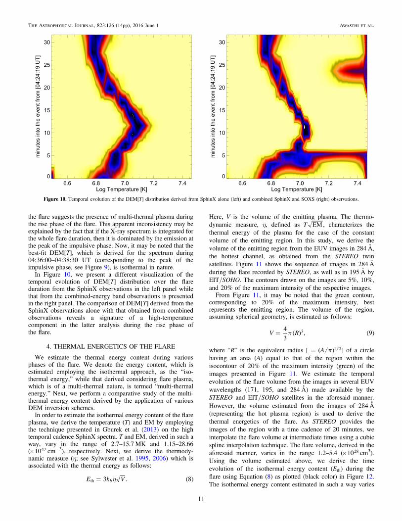
In Figure 10, we present a different visualization of thetemporal evolution of DEM[T] distribution over the flareduration from the SphinX observations in the left panel whilethat from the combined-energy band observations is presentedin the right panel. The comparison of DEM[T] derived from theSphinX observations alone with that obtained from combinedobservations reveals a signature of a high-temperaturecomponent in the latter analysis during the rise phase ofthe flare.

4. THERMAL ENERGETICS OF THE FLARE

We estimate the thermal energy content during variousphases of the flare. We denote the energy content, which isestimated employing the isothermal approach, as the “iso-thermal energy,” while that derived considering flare plasma,which is of a multi-thermal nature, is termed “multi-thermalenergy.” Next, we perform a comparative study of the multi-thermal energy content derived by the application of variousDEM inversion schemes.

In order to estimate the isothermal energy content of the flareplasma, we derive the temperature (T) and EM by employingthe technique presented in Gburek et al. (2013) on the hightemporal cadence SphinX spectra. T and EM, derived in such away, vary in the range of 2.7–15.7 MK and 1.15–28.66(́ 1047 cm−3), respectively. Next, we derive the thermody-namic measure (η; see Sylwester et al. 1995, 2006) which isassociated with the thermal energy as follows:

h=E k V3 . 8bth ( )

Here, V is the volume of the emitting plasma. The thermo-dynamic measure, η, defined as T EM , characterizes thethermal energy of the plasma for the case of the constantvolume of the emitting region. In this study, we derive thevolume of the emitting region from the EUV images in 284Å,the hottest channel, as obtained from the STEREO twinsatellites. Figure 11 shows the sequence of images in 284Åduring the flare recorded by STEREO, as well as in 195Å byEIT/SOHO. The contours drawn on the images are 5%, 10%,and 20% of the maximum intensity of the respective images.From Figure 11, it may be noted that the green contour,

corresponding to 20% of the maximum intensity, bestrepresents the emitting region. The volume of the region,assuming spherical geometry, is estimated as follows:

p=V R4

3, 93( ) ( )

where “R” is the equivalent radius [ = pA 1 2( ) ] of a circlehaving an area (A) equal to that of the region within theisocontour of 20% of the maximum intensity (green) of theimages presented in Figure 11. We estimate the temporalevolution of the flare volume from the images in several EUVwavelengths (171, 195, and 284Å) made available by theSTEREO and EIT/SOHO satellites in the aforesaid manner.However, the volume estimated from the images of 284Å(representing the hot plasma region) is used to derive thethermal energetics of the flare. As STEREO provides theimages of the region with a time cadence of 20 minutes, weinterpolate the flare volume at intermediate times using a cubicspline interpolation technique. The flare volume, derived in theaforesaid manner, varies in the range 1.2–5.4 (́ 1028 cm3).Using the volume estimated above, we derive the timeevolution of the isothermal energy content (Eth) during theflare using Equation (8) as plotted (black color) in Figure 12.The isothermal energy content estimated in such a way varies

Figure 10. Temporal evolution of the DEM[T] distribution derived from SphinX alone (left) and combined SphinX and SOXS (right) observations.

11

The Astrophysical Journal, 823:126 (14pp), 2016 June 1 Awasthi et al.

in the range (2–9) ´ 1029 erg. In a similar fashion, we alsoestimate the isothermal energy content employing the T andEM derived from the GOES observations (see Figure 2). Thusthe isothermal energy, as derived from the GOES observations,is found to vary in the range (1.5–6.5)´ 1029 erg during theflare, which is shown by the yellow plot in Figure 12.

The estimate of the source size may contain various kinds ofuncertainties, knowledge of which is crucial when investigate-ing as they subsequently propagate to the thermal energyestimates. As the EUV source sizes are used with the DEM[T]distribution (derived from X-ray observations) while estimatingthe thermal energy content, a disagreement between thecotemporal source sizes within the EUV and X-ray wavebandsmay become a major contributor to the uncertainty. Unfortu-nately, imaging mode observations in the X-ray waveband arenot available for this flare, and hence EUV images have been

used in this study for source size estimation. Although the284Å filter provides the peak temperature response (at∼2MK), maximum among the other EUV wavelengthsavailable from STEREO satellites, it is still quite far from flareplasma temperatures in which X-ray emission is obtained. Inthis regard, we estimate the co-temporal X-ray and EUV sourcesizes of 13 flares of intensity class B1.1—C1.0 which occurredduring 2009 July 04–06 in active region AR11024. It may benoted that SOL2009-07-04T04:37, the flare considered in ourpresent study, is also produced from the same active region. Inthis statistical investigation, we have used X-ray imagesobtained from HINODE/XRT and EUV images from theSTEREO twin satellites in 195Å. The source size in both theaforementioned wavelengths is estimated by employing thesame approach as discussed previously. The comparativeinvestigation has revealed that the source sizes estimated fromthe X-ray images are systematically smaller than those derivedfrom the EUV images, whereas the ratio varies in the range of1.1–9.0 with a median value of 6. Next, imaging an asymmetricflaring region with instruments that observe the Sun fromdifferent angles, e.g., the observation of AR11024 with theSTEREO-A and B satellites (Figure 3), may contribute toadditional uncertainty in the source size estimation. In view ofthis, we have also made a comparison of the EUV source sizesestimated from 195Å images obtained from the STEREO-Aand B satellites for our 13 flares. This study revealed that theorthogonal view of the flaring region systematically results in alarger source size by a factor varying in the range of 1.2–1.5than that calculated from the images with an on-disk view. Asthe uncertainty in the source size, which arises due to thedifference in EUV and X-ray source sizes, is larger than thanthat which occurred due to observing the region from differentangles, the latter may be neglected while calculating theuncertainties in the thermal energy estimates. Thus, inconclusion, considering that the EUV source sizes are system-atically larger than the X-ray sources by a factor of 6, thevolume derived from the same suffers from an overestimate bya factor of 4. Employing the error propagation scheme, theapplication of the noted uncertainty in the volume estimatesmay result in an overestimate of the thermal energy content(Equation (9)) by a factor of ∼2. We show the aforementioneduncertainty in the isothermal energy estimate in the form of theassociated filled area (light red) in Figure 12.

Figure 11. Images in 284 Å during the flare, obtained by STEREO-A and B as shown in the left and middle panels, respectively. The right panel shows the imageobtained during the flare at 195 Å from EIT/SOHO. The contours overlaid on the images correspond to 5% (red), 10% (blue), and 20% (green) of the maximumintensity regions.

Figure 12. Temporal evolution of the isothermal and multi-thermal energycontent during the flare. Isothermal energy, estimated from SphinX observa-tions, is plotted in black (smoothed in red), while that derived from GOESobservations in shown in yellow. Multi-thermal energy, derived by applyingthe W–S algorithm to the SphinX and SOXS combined data is shown as theblue histogram. The uncertainty in the estimation of the isothermal energycontent is shown by the filled area (light red) while the same corresponding tothe multi-thermal energy content is shown in the form of error bars (blue).

12

The Astrophysical Journal, 823:126 (14pp), 2016 June 1 Awasthi et al.

Next, we estimate the multi-thermal energy content of theflare with the help of the DEM[T] distribution, derived from theW–S inversion scheme, as per the following equation(Sylwester et al. 2014; Aschwanden et al. 2015b):

å=E k V T3 DEM . 10Bk

k kth1 2 1 2 ( )

The multi-thermal energy content derived in such a mannervaries in the range of (1–7) ´ 1029 erg as plotted by the bluehistogram in Figure 12. In the estimation of multi-thermalenergetics, we have employed the combined data set preparedfrom the X-ray emission in the 1.6–5.0 keV range as obtainedfrom SphinX, and in the 5.0–8.0 keV range (with theapplication of a normalization factor of “2.5”) from SOXS(see Section 3). It may be argued that this normalizationscheme is biased. In this regard, we made a parallel case studyin which the best-fit DEM[T] distribution is derived using acombined data set which, however, is prepared by applying theinverse normalization factor to the SphinX observations whileconsidering SOXS observations to be true. This investigationresulted in DEM values which are systematically lower by afactor of 2.5 compared to those estimated in the previous case.On the other hand, the best-fit plasma temperature valuesremain unchanged (also see Mrozek et al. 2012). Therefore,considering the fact that the DEM values in the former case arelarger by the noted factor, i.e., 2.5, the resulting multi-thermalenergy content was overestimated by a factor of 4 (Equa-tion (10)). In this calculation, we have also included theuncertainty in the volume estimation obtained previously. InFigure 12, we show the uncertainty in the multi-thermal energyestimates (blue) with the low error bars.

The comparison of the isothermal and multi-thermal energycontent for this flare (Figure 12) revealed that multi-thermalenergy matches well with the isothermal energy during the riseand decay phases of the flare. However, during the maximumof the impulsive phase, we note minor disagreement in the formof lower values of multi-thermal energy in comparison to theisothermal energy.

Next, we derive the multi-thermal energy from the best-fitDEM[T] distribution, obtained by employing various DEMschemes to the observed SXR spectrum in the 1.6–5.0 keV(low-energy), 5.0–8.0 keV (high-energy), and 1.6–8.0 keV(combined energy) bands during the peak of impulsive phaseof the flare (04:36:00–04:38:30 UT). The multi-thermal energyfor the low-energy band SXR emission is estimated to be 177,225, and 4.1 ´1029 erg corresponding to the the singleGaussian, power-law, and W–S DEM schemes, respectively.On the other hand, the energy content derived by employingthe aforesaid DEM schemes to the high-energy band SXR isdetermined to be 64, 65, and 1.5 ´1029 erg, respectively.Furthermore, the multi-thermal energy is 85, 91, and 4.4´1029 erg when applying the aforesaid DEM schemes to thecombined energy band SXR, respectively. By comparing theabove mentioned energy estimates, we note that the flareenergetics, estimated from the parameters derived only fromthe spectral inversion of the low-energy band of the SXRspectrum leads to higher values than that obtained fromcombined energy band case. On the other hand, the multi-thermal energies, which resulted from applying various DEMschemes to the high-energy part of SXR spectrum, areestimated to be lower than those obtained from combined-energy band SXR spectrum. This trend is consistently noted inthe energetics estimated by employing all of the

aforementioned DEM schemes. On the contrary, we find thatthe best-fit DEM[T] distribution, obtained using the DEMschemes which postulate either the single Gaussian or power-law functional dependence of DEM, leads to the overestimationof the multi-thermal energy by approximately one order incomparison to that estimated from W–S algorithm.

5. SUMMARY AND CONCLUSIONS

We investigate the thermal characteristics of the flare plasmaby analyzing X-ray emission in the energy band 1.6–8.0 keVobserved during the SOL2009-07-04T04:37 flare, which is theonly common event observed by both the SphinX and SOXSinstruments. We derive the evolution of the best-fit DEM[T]distribution during the flare by employing various DEMinversion algorithms. In addition, we have also studied thedependence of the best-fit DEM[T] corresponding to variousinput energy bands within the SXR emission. The followingare the key points of our study.

1. The best-fit DEM[T] distribution for the low-(1.6–5.0 keV), high- (5.0–8.0 keV), and combined-energybands (1.6–8.0 keV) of the X-ray emission during theflare resulted in higher values of DEMp, however, at lowTp for the low-energy band in comparison to therelatively lower values of DEMp at higher Tp obtainedby analyzing the high-energy band of the SXR.

2. We derive the time evolution of the DEM[T] distributionduring various phases of the flare by employing a W–Smaximum likelihood DEM inversion algorithm toindividual as well as combined observations from SphinXand SOXS during the flare. The results are summarized asfollows.a. The best-fit DEM[ T] distribution corresponding to the

X-ray emission during the flare onset can be wellrepresented by a single Gaussian function with a widthof ∼1MK, which suggests the flare plasma to beisothermal in nature during this phase.

b. Analysis of X-ray emission during the rise to the peakof the impulsive phase of the flare revealed thepresence of multi-thermal plasma as the correspondingbest-fit DEM[ T] curves show a double Gaussian formwith widths of ∼1.5MK.

c. The temporal evolution of the best-fit DEM[ T]distribution corresponding to the post-maximumphase of the flare can be well represented by a singleGaussian function, however, with the peak tempera-ture varying in the range ∼13.0–5.5 MK.

3. Isothermal and multi-thermal energy content is estimatedduring the flare. We find that the multi-thermal energyestimates are in close agreement with the isothermalenergy values, except during the peak of the impulsivephase of the flare where isothermal energy is estimated tobe larger than the multi-thermal energy content.

4. Multi-thermal energy is determined from the best-fitDEM[T] distribution resulting from the application ofvarious inversion schemes to the X-ray emissionmeasured during the peak of the impulsive phase of theflare. We find that the energy content estimated from theparameters derived only from spectral inversion of thelow-energy band (1.6–5.0 keV) of the SXR spectrumresult in larger values than obtained from the analysis ofthe SXR emission in combined energy band. On the

13

The Astrophysical Journal, 823:126 (14pp), 2016 June 1 Awasthi et al.

contrary, the same derived from only the high-energyband of SXR spectrum leads to lower estimates whencomparing with the energy values calculated fromcombined energy band analysis. This trend is consistentlyresulted in the thermal energetics determined from all theDEM schemes. This suggests that the observations ofSXR emission during a flare in the combined-energyband with high temporal and energy cadence is veryimportant to derive the complete thermal energetics ofthe flare.

5. The best-fit DEM[T] distribution obtained for the DEMschemes, which postulate either a single Gaussian orpower-law functional form of the DEM-Tcurve, lead toan estimation of the thermal energy content which ismuch higher, by approximately one order, than thatestimated from the W–S scheme. This can be understoodby the fact that the width of the best-fit DEM[T]distribution, obtained by employing a single-Gaussianapproach (see Figure 6) is larger than that resulting fromthe application of the W–S scheme (Figure 9). It may benoted that this disagreement between various DEMinversion schemes, and hence thermal energy estimates,can have a significant impact in the context of coronalheating from low-intensity class (micro- and nano-)flares. However, as X-ray emission covers only the high-temperature corona, recent studies focussing coronalheating energized by small intensity flares also combinemulti-wavelength observations with the X-ray emissionduring flares (Testa et al. 2014). Moreover, severaladvanced schemes of DEM inversion, namely, “DEM_-manual” (Schmelz & Winebarger 2015), “EM Lociapproach” (Cirtain et al. 2007), a combination ofGaussian and power-law functional form of DEM(Guennou et al. 2013; Aschwanden et al. 2015a), etc.,have also been employed in deriving thermal character-istics of EM during small intensity class flares. Therefore,in the future, we plan to extrapolate the application of theW–S DEM inversion scheme to the combined EUV andX-ray observations during small flares in order to conducta comparative survey of the thermal energy contentderived by the W–S method and other DEM inversionschemes.

This research has been supported by the Polish NCN grant2011/01/B/ST9/05861 and from the European CommissionsSeventh Framework Programme under grant agreement No.284461 (eHEROES project). Moreover, the research leading tothese results has received funding from the EuropeanCommunitys Seventh Framework Programme (FP7/2007-

2013) under grant agreement No. 606862 (F-CHROMA).The authors also acknowledge the open data policy of theSphinX, SOXS, SOHO, HINODE, and STEREO missions.SAO/ADS abstract service is duly acknowledged for providingthe up-to-date and well-organized bibliography. Additionally,the Coyote’s IDL programming support is acknowledged. Theauthors also thank the anonymous referee for constructivecomments which improved the manuscript.

REFERENCES

Aschwanden, M. J. 2007, ApJ, 661, 1242Aschwanden, M. J., Boerner, P., Caspi, A., et al. 2015a, SoPh, 290, 2733Aschwanden, M. J., Boerner, P., Ryan, D., et al. 2015b, ApJ, 802, 53Aschwanden, M. J., Xu, Y., & Jing, J. 2014, ApJ, 797, 50Awasthi, A. K., Jain, R., Gadhiya, P. D., et al. 2014, MNRAS, 437, 2249Benz, A. O. 2008, LRSP, 5, 1Brown, J. C. 1971, SoPh, 18, 489Caspi, A., & Lin, R. P. 2010, ApJL, 725, L161Choudhary, D. P., Gosain, S., Gopalswamy, N., et al. 2013, AdSpR, 52, 1561Cirtain, J. W., Del Zanna, G., DeLuca, E. E., et al. 2007, ApJ, 655, 598Craig, I. J. D., & Brown, J. C. 1976, A&A, 49, 239Dalmasse, K., Chandra, R., Schmieder, B., & Aulanier, G. 2015, A&A,

574, A37Delaboudinière, J.-P., Artzner, G. E., Brunaud, J., et al. 1995, SoPh, 162, 291Del Zanna, G., Dere, K. P., Young, P. R., Landi, E., & Mason, H. E. 2015,

A&A, 582, A56Dere, K. P., & Cook, J. W. 1979, ApJ, 229, 772Fletcher, L., Dennis, B. R., Hudson, H. S., et al. 2011, SSRv, 159, 19Gburek, S., Sylwester, J., Kowalinski, M., et al. 2011, SoSyR, 45, 189Gburek, S., Sylwester, J., Kowalinski, M., et al. 2013, SoPh, 283, 631Guennou, C., Auchère, F., Klimchuk, J. A., Bocchialini, K., & Parenti, S. 2013,

ApJ, 774, 31Jain, R., Aggarwal, M., & Sharma, R. 2008, JApA, 29, 125Jain, R., Awasthi, A. K., Chandel, B., et al. 2011a, SoPh, 271, 57Jain, R., Awasthi, A. K., Rajpurohit, A. S., & Aschwanden, M. J. 2011b, SoPh,

270, 137Jain, R., Dave, H., Shah, A. B., et al. 2005, SoPh, 227, 89Kepa, A., Sylwester, B., Siarkowski, M., & Sylwester, J. 2008, AdSpR,

42, 828Kepa, A., Sylwester, J., Sylwester, B., Siarkowski, M., & Stepanov, A. I. 2006,

SoSyR, 40, 294Kulinová, A., Kašparová, J., Dzifčáková, E., et al. 2011, A&A, 533, A81Landi, E., Del Zanna, G., Young, P. R., Dere, K. P., & Mason, H. E. 2012,

ApJ, 744, 99Li, H., Berlicki, A., & Schmieder, B. 2005, A&A, 438, 325Mrozek, T., Gburek, S., Siarkowski, M., et al. 2012, CEAB, 36, 71Saint-Hilaire, P., & Benz, A. O. 2005, A&A, 435, 743Schmelz, J. T., & Winebarger, A. R. 2015, RSPTA, 373, 20140257Shibata, K. 1999, Ap&SS, 264, 129Sylwester, B., Sylwester, J., Kepa, A., et al. 2006, SoSyR, 40, 125Sylwester, B., Sylwester, J., Phillips, K. J. H., Kȩpa, A., & Mrozek, T. 2014,

ApJ, 787, 122Sylwester, J., Garcia, H. A., & Sylwester, B. 1995, A&A, 293, 577Sylwester, J., Kowalinski, M., Gburek, S., et al. 2012, ApJ, 751, 111Sylwester, J., Schrijver, J., & Mewe, R. 1980, SoPh, 67, 285Testa, P., De Pontieu, B., Allred, J., et al. 2014, Sci, 346, 1255724

14

The Astrophysical Journal, 823:126 (14pp), 2016 June 1 Awasthi et al.