THEORY OF THIN PLATES AND SHELLS

Mr. Gude Ramakrishna Associate Profesor

by

Outline

2

The concepts of Space Curves, surfaces, shell co-ordinates, boundary conditions.

The governing equation for a rectangular plate, Navier solution for simply- supported rectangular plate under various loadings.

Analyze , understand axi- symmetric loading, governing differential equation in polar co-ordinates.

The cylindrical and conical shells, application to pipes and pressure vessels. and understand the membrane theory of cylindrical.

UNIT-I

INTRODUCTION

•

Thin shells as structural elements occupy a leadershipposition in engineering and, in particular, in civil,mechanical, architectural, aeronautical, and marineengineering.

• Examples of shell structures in civil and architecturalengineering are large-span roofs, liquid-retainingstructures and water tanks, containment shells of nuclearpower plants, and

SHELLS IN ENGINEERING STRUCTURES

• concrete arch domes. In mechanical engineering, shell formsare used in piping systems, turbine disks, and pressurevessels technology. Aircrafts, missiles, rockets, ships, andsubmarines are examples of the use of shells in aeronauticaland marine engineering.

• Another application of shell engineering is in the field ofbiomechanics: shells are found in various biological forms,such as the eye and the skull, and plant and animal shapes.This is only a small list of shell forms in engineering andnature.

• Strategic cost management is understood in different ways in literature. Cooper and Slag Mulder argued that strategic cost management is “the application of cost management techniques so that they simultaneously improve the strategic position of a firm and reduce costs”.

• A hospital redesigns its patient admission procedure so it becomes more efficient and easier for patients. The hospital will become known for its easy admission procedure so more people will come to that hospital if the patient has a choice.

ADVANTAGES

• In addition to these mechanical advantages, shell structuresenjoy the unique position of having extremely high aestheticvalue in various architectural designs.

• Shell structures support applied external forcesefficiently by virtue of their geometrical form, i.e., spatialcurvatures; as a result, shells are much stronger and stifferthan other structural forms

BUSINESS STRATEGY & STRATEGIC COST MANAGEMENTExamples

We now formulate some definitions and principles in shell

theory. The term shell is applied to bodies bounded by twocurved surfaces, where the distance between the surfaces issmall in comparison with other body dimensions fig shownbelow

GENERAL DEFINITIONS AND FUNDAMENTALS OF SHELLS

The locus of points that lie at equal distances from these twocurved surfaces defines the middle surface of the shell. Thelength of the segment, which is perpendicular to the curvedsurfaces, is called the thickness of the shell and is denoted by h.

The geometry of a shell is entirely defined by specifying theform of the middle surface and thickness of the shell at eachpoint. In this book we consider mainly shells of a constantthickness. Shells have all the characteristics of plates, along withan additional one – curvature.

The curvature could be chosen as the primary classifier of ashell because a shell’s behavior under an applied loading isprimarily governed by curvature .

Depending on the curvature of the surface, shells aredivided into cylindrical (noncircular and circular), conical,spherical, ellipsoidal, paraboloidal, toroidal, and hyperbolicparaboloidal shells. Owing to the curvature of the surface,shells are more complicated than flat plates because theirbending cannot, in general, be separated from theirstretching.

On the other hand, a plate may be considered as a speciallimiting case of a shell that has no curvature; consequently,shells are sometimes referred to as curved plates. This is thebasis for the adoption of methods from the theory of plates,discussed in Part I, into the theory of shells.

There are two different classes of shells: thick shells and thinshells. A shell is called thin if the maximum value of the ratio h=R(where R is the radius of curvature of the middle surface) can beneglected in comparison with unity. For an engineering accuracy,a shell may be regarded as thin if [1] the following condition issatisfied:

Max (h/ R) <or=1/20

Hence, shells for which this inequality is violated are referredto as thick shells. For a large number of practical applications,the thickness of shells lies in the range

(1/1000) <or=(h/R)<or=1/20

The most common shell theories are those based onlinear elasticity concepts. Linear shell theories predictadequately stresses and deformations for shells exhibitingsmall elastic deformations; i.e., deformations for which it isassumed that the equilibrium equation conditions fordeformed shell surfaces are the same as if they were notdeformed, and Hooke’s law applies.

For the purpose of analysis, a shell may be consideredas a three-dimensional body, and the methods of thetheory of linear elasticity may then be applied.

THE LINEAR SHELL THEORIES

However, a calculation based on these methods willgenerally be very difficult and complicated. In the theory ofshells, an alternative simplified method is thereforeemployed. According to this method and adapting somehypotheses the 3D problem of shell equilibrium andstraining may be reduced to the analysis of its middlesurface only, i.e. the given shell, as discussed earlier as a thinplate, may be regarded as some 2D body.

In the development of thin shell theories,simplification is accomplished by reducing the shellproblems to the study of deformations of the middlesurface.

Shell theories of varying degrees of accuracy were derived,depending on the degree to which the elasticity equations weresimplified. The approximations necessary for the development ofan adequate theory of shells have been the subject ofconsiderable discussions among investigators in the field. Wepresent below a brief outline of elastic shell.

A second class of thin elastic shells, which is commonlyreferred to as higher order approximation, has also beendeveloped. To this grouping it is possible to assign all linear shelltheories in which one or another of the Kirchhoff–Lovehypotheses are suspended. First, we consider somerepresentative theories in which the thinness assumption isdelayed in derivation while the rest of the postulates are

The membrane stress condition is an ideal state at which a

designer should aim. It should be noted that structuralmaterials are generally far more efficient in an extensionalrather in a flexural mode because:

1. Strength properties of all materials can be usedcompletely in tension (or compression), since all fibers overthe cross section are equally strained and load-carryingcapacity may simultaneously reach the limit for the wholesection of the component.

2. The membrane stresses are always less than thecorresponding bending

A surface can be defined as a locus of points whoseposition vector, r, directed from the origin 0 of the globalcoordinate system, OXYZ, is a function of two independentparameters α and β

COORDINATE SYSTEM OF THE SURFACE

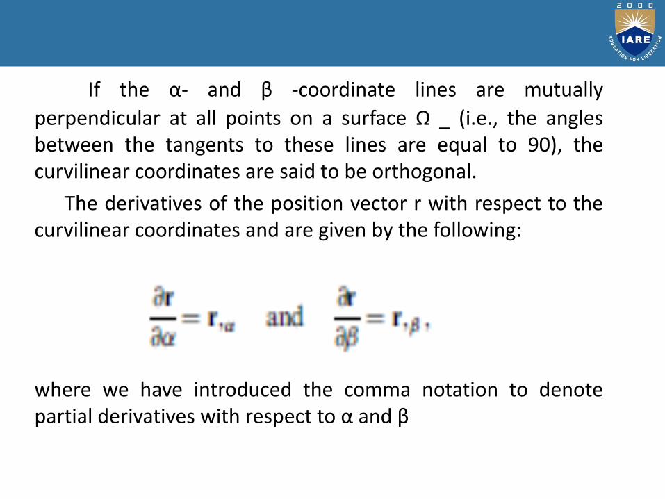
If the α- and β -coordinate lines are mutually

perpendicular at all points on a surface Ω _ (i.e., the anglesbetween the tangents to these lines are equal to 90), thecurvilinear coordinates are said to be orthogonal.

The derivatives of the position vector r with respect to thecurvilinear coordinates and are given by the following:

where we have introduced the comma notation to denotepartial derivatives with respect to α and β

Assume that the elastic body shown in Fig. below is supportedin such a way that rigid body displacements (translations androtations) are prevented. Thus, this body deforms under theaction of external forces and each of its points has small elasticdisplacements. For example, a point M had the coordinates x; y,and z in initial unreformed state. After deformation, this pointmoved into position M0and its coordinates became the following

where u, v, and w are projections of the displacementvector of point M, vector MM0, on the coordinate axes x, y andz. In the general case, u, v, and w are functions of x, y, and z.

STRAINS AND DISPLACEMENTS

Again, consider an infinitesimal element in the form ofparallelepiped enclosing point of interest M. Assuming that adeformation of this parallelepiped is small, we can represent it inthe form of the six simplest deformations shown in Fig. a,b,c,d.define the elongation (or contraction) of edges of theparallelepiped in the direction of the coordinate axes and can bedefined as

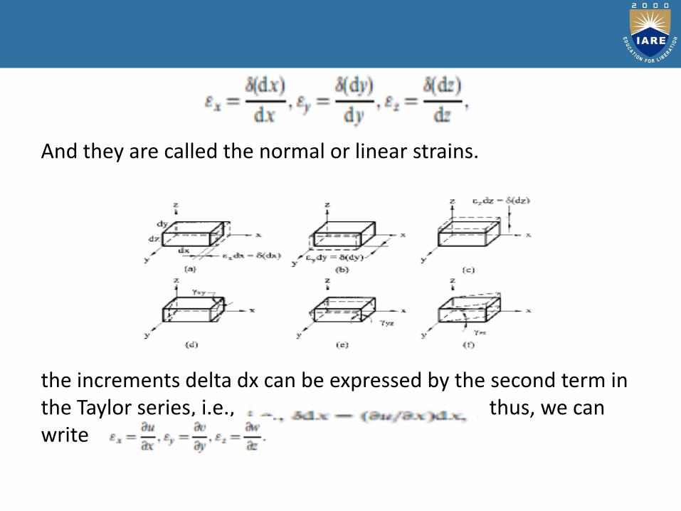
And they are called the normal or linear strains.

the increments delta dx can be expressed by the second term in the Taylor series, i.e., thus, we can write

Since we have confined ourselves to the case of very smalldeformations, we may omit the quantities in thedenominator of the last expression, as being negligibly smallcompared with unity. Finally, we obtain

Similarly, we can obtain _xz and _yz. Thus, the shear

strains are given by

Similar to the stress tensor at a given point, we can define a strain tensor as

It is evident that the strain tensor is also symmetric because of

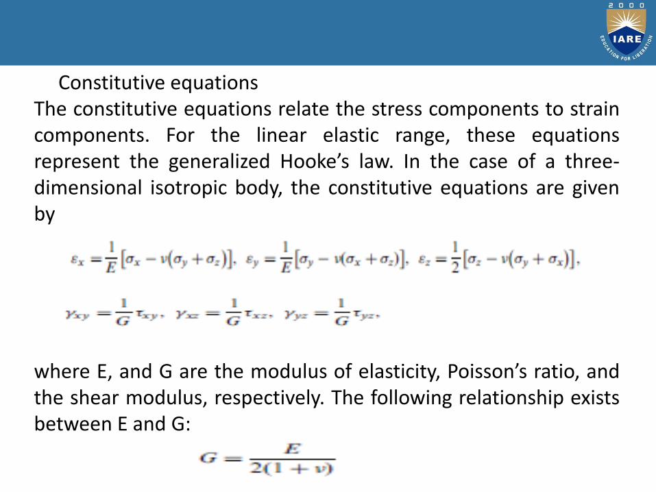
Constitutive equationsThe constitutive equations relate the stress components to straincomponents. For the linear elastic range, these equationsrepresent the generalized Hooke’s law. In the case of a three-dimensional isotropic body, the constitutive equations are givenby

where E, and G are the modulus of elasticity, Poisson’s ratio, andthe shear modulus, respectively. The following relationship existsbetween E and G:

The stress components introduced previously must satisfythe following differential equations of equilibrium:

where Fx; Fy; and Fz are the body forces (e.g., gravitational,magnetic forces). In deriving these equations, the reciprocity ofthe shear stresses, Eqs , has been used.

EQUILIBRIUM EQUATIONS

UNIT – II

STATIC ANALYSIS OF PLATES

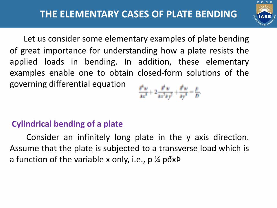
Let us consider some elementary examples of plate bending

of great importance for understanding how a plate resists theapplied loads in bending. In addition, these elementaryexamples enable one to obtain closed-form solutions of thegoverning differential equation

Cylindrical bending of a plate

Consider an infinitely long plate in the y axis direction.Assume that the plate is subjected to a transverse load which isa function of the variable x only, i.e., p ¼ pðxÞ

THE ELEMENTARY CASES OF PLATE BENDING

In this case all the strips of a unit width parallel to the x axis andisolated from the plate will bend identically. The plate as a whole isfound to be bent over the cylindrical surface w ¼ wðxÞ. Setting allthe derivatives with respect to y equal zero in Eq

we obtain the following equation for the deflection:

An integration of Eq. should present no problems. Let, for example,p ¼ p0xa, then the general solution of Eq. is of the following form:

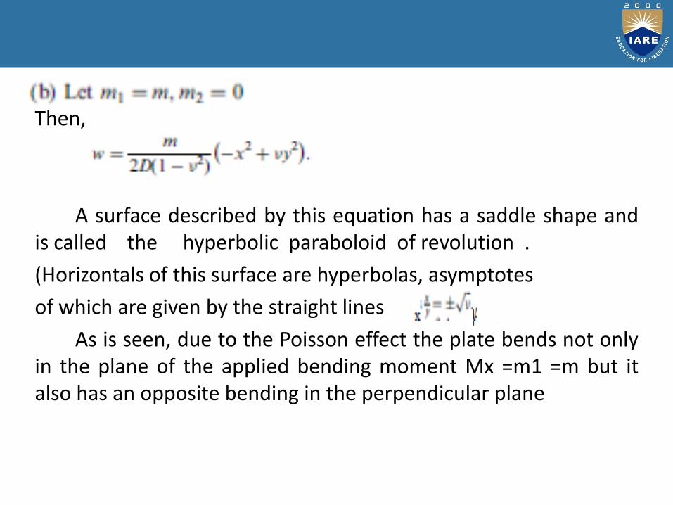
Then,

A surface described by this equation has a saddle shape andis called the hyperbolic paraboloid of revolution .

(Horizontals of this surface are hyperbolas, asymptotes

of which are given by the straight lines

As is seen, due to the Poisson effect the plate bends not onlyin the plane of the applied bending moment Mx =m1 =m but italso has an opposite bending in the perpendicular plane

Then

Thus, a part of the plate isolated from the whole plate andequally inclined to the x and y axes will be loaded along itsboundary by uniform twisting moments of intensity m. Hence,this part of the plate is subjected to pure twisting

Let us replace the twisting moments by the effective shearforces Vα rotating these moments through 90. Along the wholesides of the isolated part we obtain Vα=0, but at the cornerpoints the concentrated forces S ¼ 2m are applied. Thus, for themodel of Kirchhoff’s plate, an application of self-balancedconcentrated forces at corners of a rectangular plate produces adeformation of pure torsion because over the whole surface ofthe plate

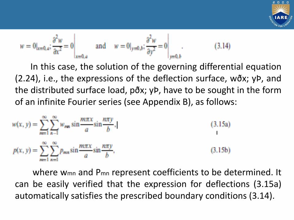
In this case, the solution of the governing differential equation(2.24), i.e., the expressions of the deflection surface, wðx; yÞ, andthe distributed surface load, pðx; yÞ, have to be sought in the formof an infinite Fourier series (see Appendix B), as follows:

where wmn and Pmn represent coefficients to be determined. Itcan be easily verified that the expression for deflections (3.15a)automatically satisfies the prescribed boundary conditions (3.14).

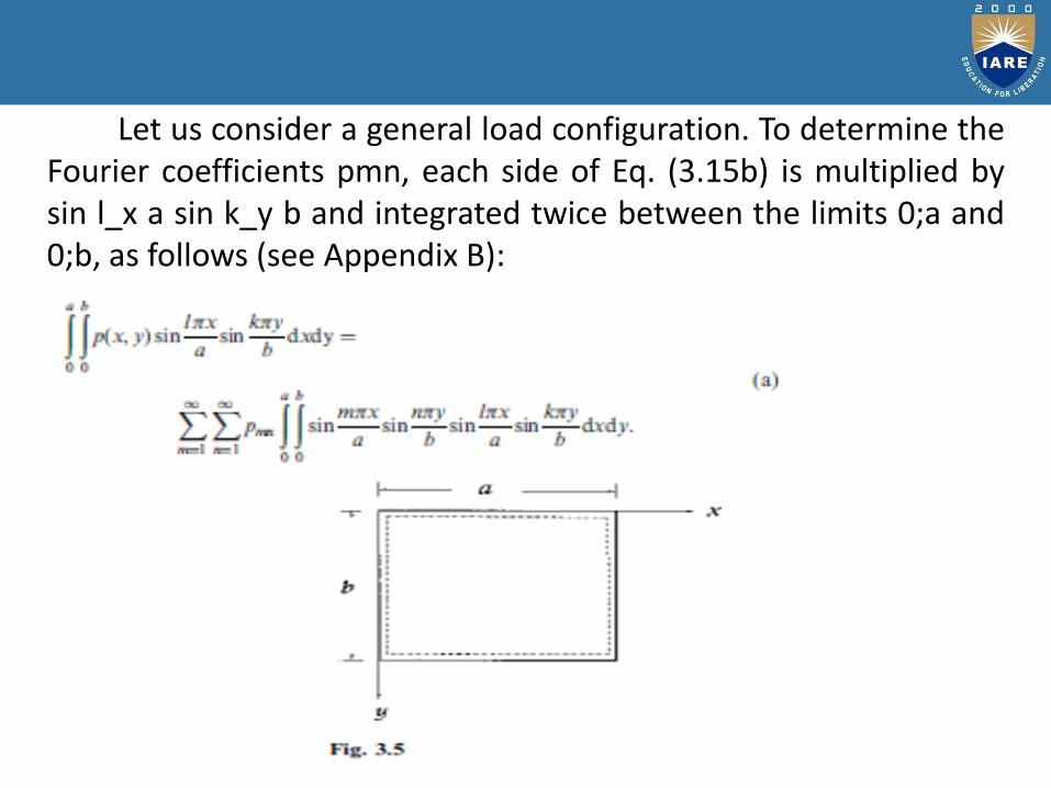
Let us consider a general load configuration. To determine theFourier coefficients pmn, each side of Eq. (3.15b) is multiplied bysin l_x a sin k_y b and integrated twice between the limits 0;a and0;b, as follows (see Appendix B):

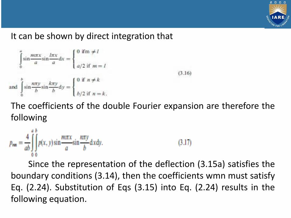
It can be shown by direct integration that

The coefficients of the double Fourier expansion are therefore thefollowing

Since the representation of the deflection (3.15a) satisfies theboundary conditions (3.14), then the coefficients wmn must satisfyEq. (2.24). Substitution of Eqs (3.15) into Eq. (2.24) results in thefollowing equation.

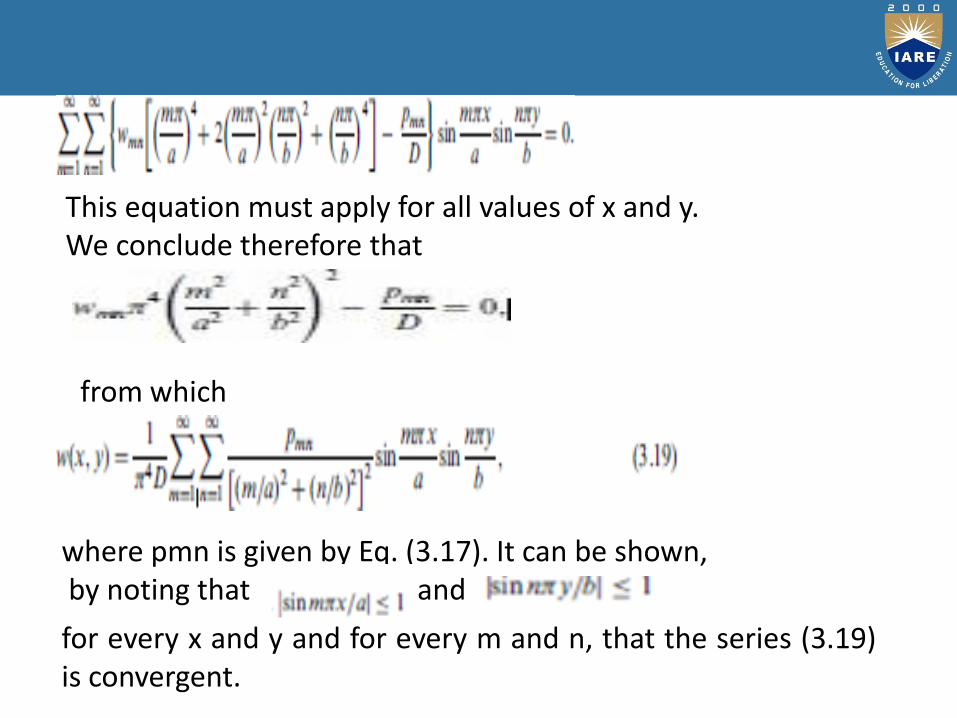
This equation must apply for all values of x and y.We conclude therefore that

from which

where pmn is given by Eq. (3.17). It can be shown,by noting that and

for every x and y and for every m and n, that the series (3.19)is convergent.

Since the stress resultants and couples are obtained fromthe second and third derivatives of the deflection wðx; yÞ, theconvergence of the infinite series expressions of the internalforces and moments is less rapid, especially in the vicinity of theplate edges. This slow convergence is also accompanied bysome loss of accuracy in the process of calculation. The accuracyof solutions and the convergence of series expressions of stressresultants and couples can be improved by considering moreterms in the expansions and by using a special technique for animprovement of the convergence of Fourier’s series.

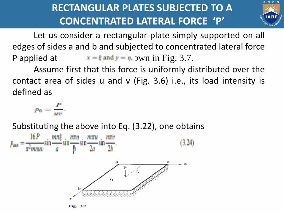
Let us consider a rectangular plate simply supported on alledges of sides a and b and subjected to concentrated lateral forceP applied at as shown in Fig. 3.7.

Assume first that this force is uniformly distributed over thecontact area of sides u and v (Fig. 3.6) i.e., its load intensity isdefined as

Substituting the above into Eq. (3.22), one obtains

RECTANGULAR PLATES SUBJECTED TO A CONCENTRATED LATERAL FORCE ‘P’

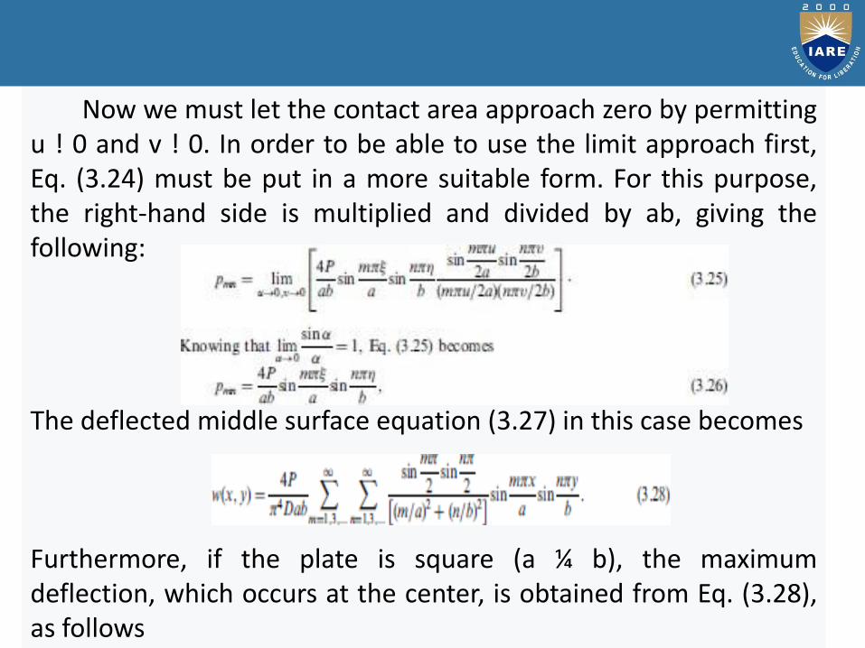
Now we must let the contact area approach zero by permittingu ! 0 and v ! 0. In order to be able to use the limit approach first,Eq. (3.24) must be put in a more suitable form. For this purpose,the right-hand side is multiplied and divided by ab, giving thefollowing:

The deflected middle surface equation (3.27) in this case becomes

Furthermore, if the plate is square (a ¼ b), the maximumdeflection, which occurs at the center, is obtained from Eq. (3.28),as follows

Retaining the first nine terms of this serieswe obtain

The ‘‘exact’’ value is and the error is thus 1.5% [3].This very simple Navier’s solution, Eq. (3.28), converges

sufficiently rapidly for calculating the deflections. However, it isunsuitable for calculating the bending moments and stressesbecause the series for the second derivatives andobtained by differentiating the series (3.28) converge extremelyslowly. These series for bending moment, and consequently forstresses as well as for the shear forces, diverge directly at a pointof application of a concentrated force, called a singular point.

In the preceding sections it was shown that the calculation ofbending moments and shear forces using Navier’s solution is notvery satisfactory because of slow convergence of the series.

In 1900 Levy developed a method for solving rectangularplate bending problems with simply supported two oppositeedges and with arbitrary conditions of supports on the tworemaining opposite edges using single Fourier series [8]. Thismethod is more practical because it is easier to perform numericalcalculations for single series that for double series and it is alsoapplicable to plates with various boundary conditions.

Levy suggested the solution of Eq. (2.24) be expressed interms of complementary , wh ; and particular, wp , parts, each ofwhich consists of a single Fourier series where unknown functionsare determined from the prescribed boundary conditions. Thus,the solution is expressed as follows:

LEVY’S SOLUTION (SINGLE SERIES SOLUTION)

Consider a plate with opposite edges, x ¼ 0 and x ¼ a, simplysupported, and two remaining opposite edges, y ¼ 0 and y ¼ b,which may have arbitrary supports.

The boundary conditions on the simply supported edges are

As mentioned earlier, the second boundary condition can bereduced to the following form:

The complementary solution is taken to be

where fmðyÞ is a function of y only; wh also satisfies the simplysupported boundary conditions (3.41). Substituting (3.42) into thefollowing homogeneous differential equation

Gives

which is satisfied when the bracketed term is equal to zero. Thus,

The solution of this ordinary differential equation can be expressed as

Substituting the above into Eq. (3.44), gives the followingcharacteristic equation

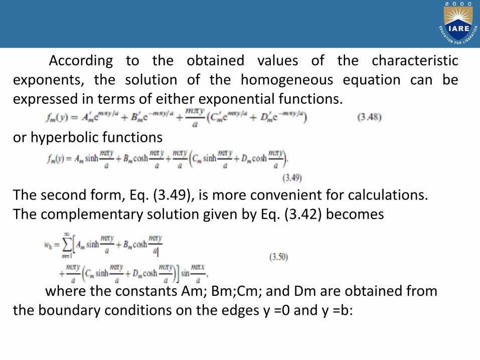
According to the obtained values of the characteristicexponents, the solution of the homogeneous equation can beexpressed in terms of either exponential functions.

or hyperbolic functions

The second form, Eq. (3.49), is more convenient for calculations.The complementary solution given by Eq. (3.42) becomes

where the constants Am; Bm;Cm; and Dm are obtained from the boundary conditions on the edges y =0 and y =b:

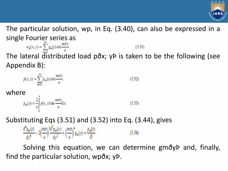
The particular solution, wp, in Eq. (3.40), can also be expressed in asingle Fourier series as

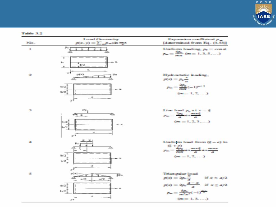
The lateral distributed load pðx; yÞ is taken to be the following (seeAppendix B):

where

Substituting Eqs (3.51) and (3.52) into Eq. (3.44), gives

Solving this equation, we can determine gmðyÞ and, finally,find the particular solution, wpðx; yÞ.

CONTINUOUS PLATES

When a uniform plate extends over a support and has morethan one span along its length or width, it is termed continuous.Such plates are of considerable practical interest. Continuousplates are externally statically indeterminate members (note that aplate itself is also internally statically indeterminate). So, the well-known methods developed in structural mechanics can be used forthe analysis of continuous plates.

In this section, we consider the force method which iscommonly used for the analysis of statically indeterminatesystems. According to this method, the continuous plate issubdivided into individual, simple-span panels betweenintermediate supports by removing all redundant restraints. It canbe established, for example, by introducing some fictitious hingesabove the intermediate supports.

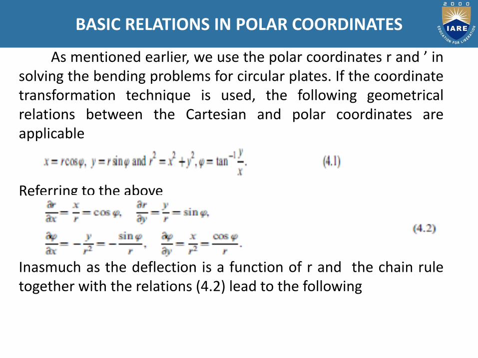
As mentioned earlier, we use the polar coordinates r and ’ insolving the bending problems for circular plates. If the coordinatetransformation technique is used, the following geometricalrelations between the Cartesian and polar coordinates areapplicable

Referring to the above

Inasmuch as the deflection is a function of r and the chain ruletogether with the relations (4.2) lead to the following

BASIC RELATIONS IN POLAR COORDINATES

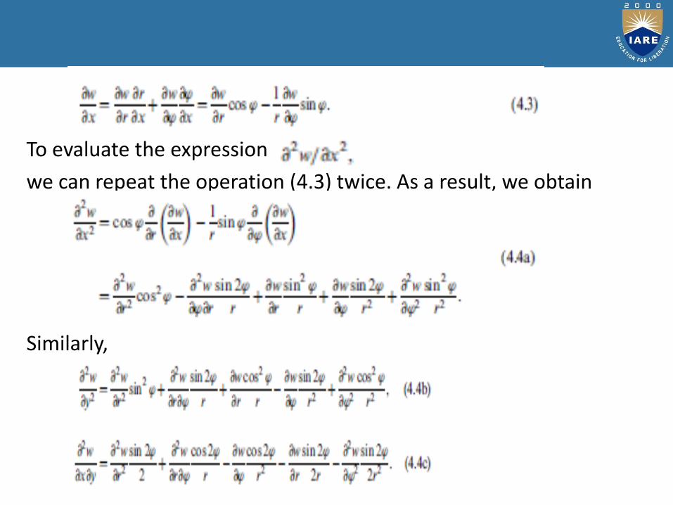
To evaluate the expression

we can repeat the operation (4.3) twice. As a result, we obtain

Similarly,

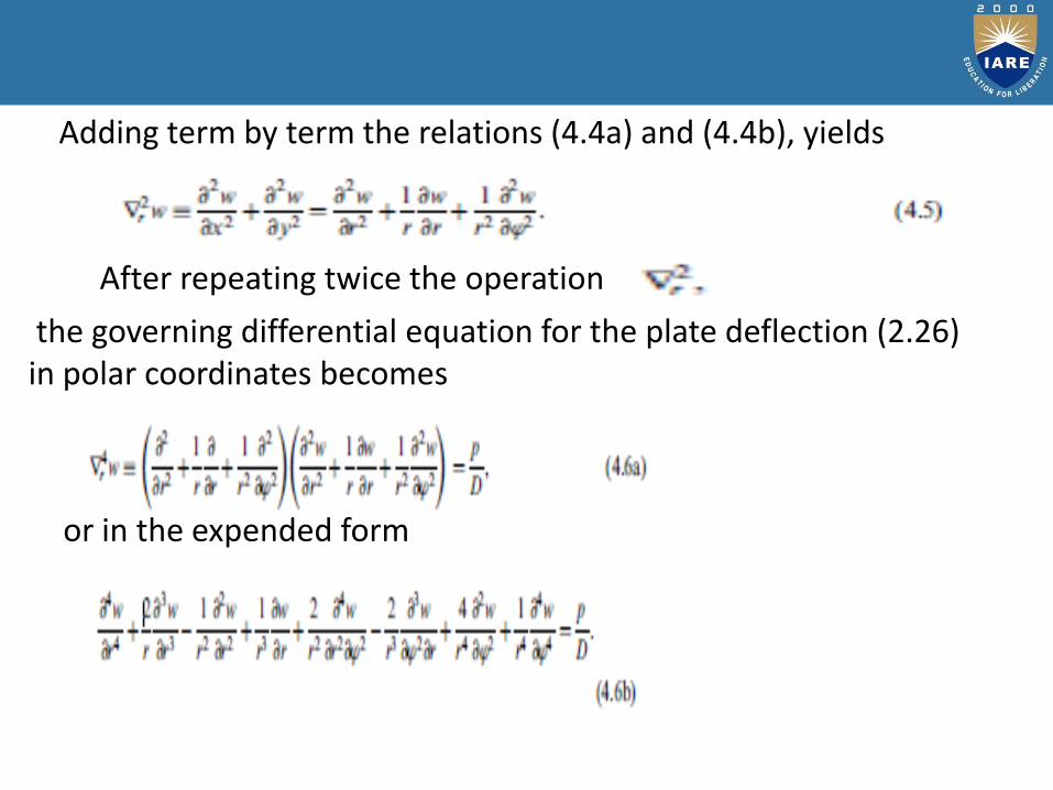
Adding term by term the relations (4.4a) and (4.4b), yields

After repeating twice the operation

the governing differential equation for the plate deflection (2.26)in polar coordinates becomes

or in the expended form

Let us set up the relationships between moments and

curvatures. Consider now the state of moment and shear force on an

infinitesimal element of thickness h, described in polar coordinates,

as shown in Fig. 4.1b. Note that, to simplify the derivations, the x

axis is taken in the direction of the radius r, at ’ ¼ 0 (Fig. 4.1b).

Then, the radialMr, tangential Mt, twisting Mrt moments, and the

vertical shear forces Qr;Qt will have the same values as the

moments Mx;My; and Mxy, and shears Qx;Qy at the same point in

the plate. Thus, transforming the expressions for moments (2.13)

and shear forces (2.27) into polar coordinates, we can write the

following:

Similarly, the formulas for the plane stress components

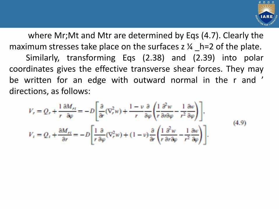
where Mr;Mt and Mtr are determined by Eqs (4.7). Clearly themaximum stresses take place on the surfaces z ¼ _h=2 of the plate.

Similarly, transforming Eqs (2.38) and (2.39) into polarcoordinates gives the effective transverse shear forces. They maybe written for an edge with outward normal in the r and ’directions, as follows:

UNIT – IV

STATIC ANALYSIS OF SHELLS: MEMBRANE THEORY OF SHELLS

We define here some of the surfaces that are commonlyused for shell structures in engineering practice. There areseveral possible classifications of these surfaces. One suchclassification, associated with the Gaussian curvature, wasdiscussed in Sec. 11.6. Following Ref. [4], we now discuss othercategories of shell surfaces associated with their shape andgeometric develop ability.

Classification based on geometric form(a) Surfaces of revolution

(b) Surfaces of translation(c) Ruled surfaces

CLASSIFICATION OF SHELL SURFACES

(a) Surfaces of revolution (Fig. 11.9)

As mentioned previously, surfaces of revolution aregenerated by rotating a plane curve, called the meridian, about anaxis that is not necessarily intersecting the meridian. Circularcylinders, cones, spherical or elliptical domes, hyperboloids ofrevolution, and toroids (see Fig. 11.9) are some examples ofsurfaces of revolution. It can be seen that for the circular cylinderand cone (Fig. 11.9a and b), the meridian is a straight line, andhence, k1 ¼ 0, which gives _¼ 0. These are shells of zero

Gaussian curvature. For ellipsoids and paraboloids ofrevolution and spheres (Fig. 11.9c, d, and e), both the principalcurvatures are in the same direction and, thus, these surfaces havea positive Gaussian curvature (_ > 0).

Classification based on geometric form

(b) Surfaces of translation (Fig. 11.10)

A surface of translation is defined as the surface generated bykeeping a plane curve parallel to its initial plane as we move italong another plane curve. The two planes containing the twocurves are at right angles to each other. An elliptic paraboloid isshown in Fig. 11.10 as an example of such a type of surfaces. It isobtained by translation of a parabola on another parabola; bothparabolas have their curvatures in the same direction. Therefore,this shell has a positive Gaussian curvature. For this surfacesections x ¼ constant and y ¼ constant are parabolas, whereas asection z ¼ constant represents an ellipse: hence its name,‘‘elliptic paraboloid.’’

(c) Ruled surfaces (Fig. 11.11)

Ruled surfaces are obtained by the translation of straightlines over two end curves (Fig. 11.11). The straight lines are notnecessarily at right angles to the planes containing the endcurves. The frustum of a cone can thus be considered as a ruledsurface, since it can be generated by translation of a straight line(the generator) over two curves at its ends. It is also, of course,a shell of revolution. The hyperboloid of revolution of one sheet,shown in Fig. 11.11a, represents another example of ruledsurfaces. It can be generated also by the translation of a straightline over two circles at its ends. Figure 11.11b shows a surfacegenerated by a translation of a straight line on a circular curve atone end and on a straight line at the other end. Such surfacesare referred to as conoids. Both surfaces shown in Fig. 11.11have negative Gaussian curvatures. 11.7.2 Classification basedon shell curvature

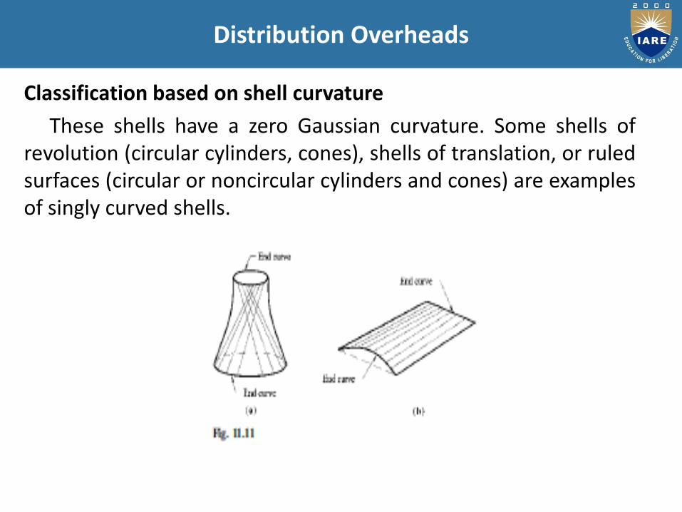
Classification based on shell curvature

These shells have a zero Gaussian curvature. Some shells ofrevolution (circular cylinders, cones), shells of translation, or ruledsurfaces (circular or noncircular cylinders and cones) are examplesof singly curved shells.

Distribution Overheads

(b) Doubly curved shells of positive Gaussian curvature

Some shells of revolution (circular domes, ellipsoids andparaboloids of revolution) and shells of translation and ruledsurfaces (elliptic paraboloids, paraboloids of revolution) can beassigned to this category of surfaces.

(c) Doubly curved shells of negative Gaussian curvature

This category of surfaces consists of some shells of revolution(hyperboloids of revolution of one sheet) and shells of translationor ruled surfaces (paraboloids,conoids, hyperboloids of revolutionof one sheet).It is seen from this classification that the same typeof shell may appear in more than one category.

(a) Developable surfaces

Developable surfaces are defined as surfaces that can be‘‘developed’’ into a plane form without cutting and/or stretching theirmiddle surface. All singly curved surfaces are examples ofdevelopable surfaces.

(b) Non-developable surfaces

A non-developable surface is a surface that has to be cut and/orstretched in order to be developed into a planar form. Surfaces withdouble curvature are usually non developable. The classification ofshell surfaces into developable and non-developable has a certainmechanical meaning. From a physical point of view, shells with non-developable surfaces require more external energy to be deformedthan do developable shells, i.e., to collapse into a plane form. Hence,one may conclude that non-developable shells are, in general,stronger and more stable than the corresponding developable.

CLASSIFICATION BASED ONGEOMETRICAL DEVELOP ABILITY

It is shown in the next chapter that the governing equations and

relations of the general theory of thin shells are formulated interms of the Lame´ parameters A and B as well as of the principalcurvatures _1 ¼ 1=R1 and _2 ¼ 1=R2. In the general case of shellshaving an arbitrary geometry of the middle surface, thecoefficients of the first and second quadratic forms and theprincipal curvatures are some functions of the curvilinearcoordinates. We determine the Lame´ parameters for some shellgeometries that are commonly encountered in engineeringpractice

SPECIALIZATION OF SHELL GEOMETRY

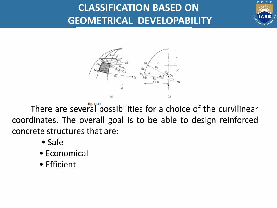
The shells of revolution were discussed in Secs 11.2 and 11.7.As for the curvilinear coordinate lines and , the meridians andparallels may be chosen: they are the lines of principal curvaturesand form an orthogonal mesh on the shell middle surface. Figure11.12a shows a surface of revolution where R1 is the principalradius of the meridian, R2 is the principal radius of the parallelcircle (as shown in Sec.11.2, R2 is the distance along a normal tothe meridional curve drawn from a point of interest to the axis ofrevolution of the surface), and r is the radius of the parallel circle.

Shells of revolution

CLASSIFICATION BASED ONGEOMETRICAL DEVELOPABILITY

There are several possibilities for a choice of the curvilinearcoordinates. The overall goal is to be able to design reinforcedconcrete structures that are:

• Safe• Economical• Efficient

Reinforced concrete is one of the principal buildingmaterials used in engineered structures because:

• Low cost

• Weathering and fire resistance

• Good compressive strength

• Formability

• Identify the regions where the beam shall be designed as aflanged and where it will be rectangular in normal slab beamconstruction,

• Define the effective and actual widths of flanged beams,

• State the requirements so that the slab part is effectivelycoupled with the flanged beam,

• Write the expressions of effective widths of T and L-beamsboth for continuous and isolated cases,

• Derive the expressions of C, T and Mu for four different casesdepending on the location of the neutral axis and depth of theflange.

Roofs and decks are mostly cast monolithic from the bottomof the beam to the top of the slab. Such rectangular beamshaving slab on top are different from others having either no slab(bracings of elevated tanks, lintels etc.) or having disconnectedslabs as in some pre-cast systems (Figs. 5.10.1 a, b and c). Due tomonolithic casting, beams and a part of the slab act together.Under the action of positive bending moment, i.e., between thesupports of a continuous beam, the slab, up to a certain length.

Width greater than the width of the beam, forms the toppart of the beam. Such beams having slab on top of therectangular rib are designated as the flanged beams - either T orL type depending on whether the slab is on both sides or on oneside of the beam (Figs. 5.10.2 a to e) . Over the supports of acontinuous beam, the bending moment is negative and the slab,therefore, is in tension while a part of the rectangular beam (rib)is in compression.

The governing equations of the membrane theory can beobtained directly from the equations of the general theory of thinshells derived in Chapter 12. For this purpose, it is assumed that,in view of the smallness of the changes of curvature and twist, the

moment terms in the equations of equilibrium for a shell elementare unimportant, although in principle the shell may resist theexternal loads in bending. Note that neglecting the moments leadsto neglecting the normal shear forces. Thus, for the membranetheory of thin shells, we can assume that

M1 = M2 = H = Q1 = Q2 = 0, (13:3)

Introducing Eq. (13.3) into Eqs below

THE FUNDAMENTAL EQUATIONS OF THE MEMBRANETHEORY OF THIN SHELLS

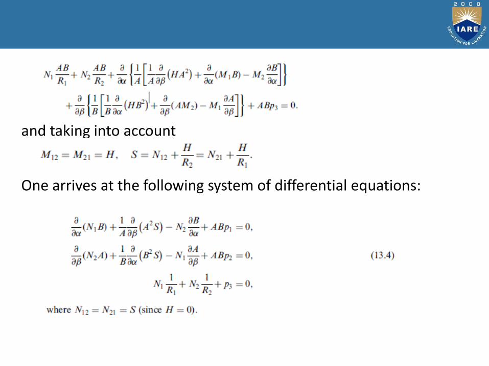
and taking into account

One arrives at the following system of differential equations:

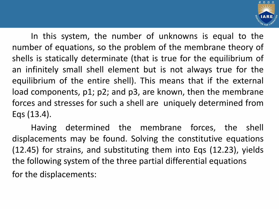
In this system, the number of unknowns is equal to thenumber of equations, so the problem of the membrane theory ofshells is statically determinate (that is true for the equilibrium ofan infinitely small shell element but is not always true for theequilibrium of the entire shell). This means that if the externalload components, p1; p2; and p3, are known, then the membraneforces and stresses for such a shell are uniquely determined fromEqs (13.4).

Having determined the membrane forces, the shelldisplacements may be found. Solving the constitutive equations(12.45) for strains, and substituting them into Eqs (12.23), yieldsthe following system of the three partial differential equations

for the displacements:

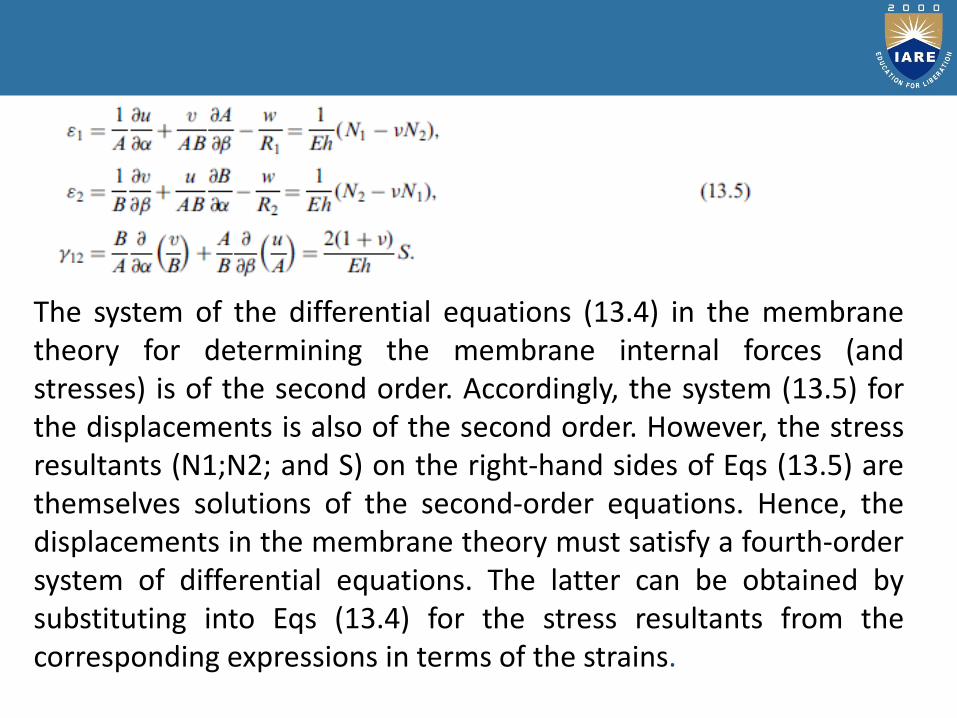
The system of the differential equations (13.4) in the membranetheory for determining the membrane internal forces (andstresses) is of the second order. Accordingly, the system (13.5) forthe displacements is also of the second order. However, the stressresultants (N1;N2; and S) on the right-hand sides of Eqs (13.5) arethemselves solutions of the second-order equations. Hence, thedisplacements in the membrane theory must satisfy a fourth-ordersystem of differential equations. The latter can be obtained bysubstituting into Eqs (13.4) for the stress resultants from thecorresponding expressions in terms of the strains.

The mathematical formulation of the theory of membraneshells is completed by adding appropriate boundary conditions. Inthe membrane theory, it follows from the above that only twoboundary conditions may be specified on each edge of the shell. Ifthe boundary conditions are given in terms of the stress resultants,

then only the membrane (or in-plane) forces (N1;N2; and S) arespecified on edges of the shell. If the boundary conditions areformulated in terms of displacements, then only displacementcomponents that are tangent to the middle surface, i.e., u and v,

must be prescribed on the shell boundary. In the membranetheory it is impossible to specify the edge displacements w andslopes #, since their assignment may result in the appearance ofthe corresponding boundary transverse shear forces and bending

moments. This is in a conflict with the general postulates of themembrane theory of thin shells introduced above.

Consider a particular case of a shell described by a surface of

revolution (Fig. 11.12).The mid surface of such a shell of revolution,as mentioned in Sec. 11.8, is generated by rotating a meridian curveabout an axis lying in the plane of this curve (the Z axis).

The geometry of shells of revolution is addressed in Sec. 11.8.There it is mentioned that meridians and parallel circles can bechosen as the curvilinear coordinate lines for such a shell becausethey are lines of curvature, and form an orthogonal mesh on its midsurface. Let us locate a point on the middle surface by the sphericalcoordinates and ’ (see Sec. 11.8), where is the circumferentialangle characterizing a position of a point along the parallel circle,whereas the angle ’ is the meridional angle, defining a position ofthat point along the meridian. The latter represents the anglebetween the normal to the middle surface and the shell axis (Fig.11.12a).

THE MEMBRANE THEORY OF SHELLS OF REVOLUTION

As before, R1;R2 are the principal radii of curvature of themeridian and parallel circle, respectively, and r is the radius of theparallel circle. The Lame´

parameters for shells of revolution in the above-mentioned sphericalcoordinate system are given by Eqs (11.39). Notice that, due to thesymmetry of shells of revolution about the Z axis, these parametersare functions of ’ only and do not depend upon �. Referring to Fig.11.12a and b, we can obtain by inspection the following relations:

Substituting for A and B from Eqs (11.39) into the system ofdifferential equations (13.4) and taking into account the relations(13.6), yields

The last equation in the above system is known as the Laplace equation. Note that the membrane forces N1;N2; and S are, in a general case of loading, some functions of

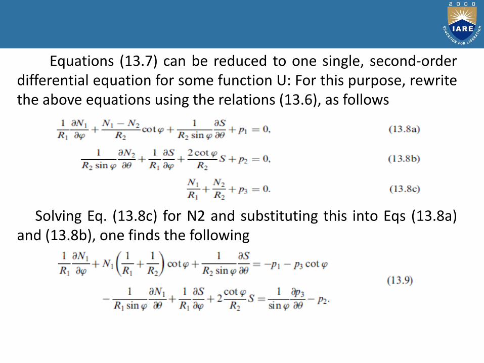
Equations (13.7) can be reduced to one single, second-orderdifferential equation for some function U: For this purpose, rewritethe above equations using the relations (13.6), as follows

Solving Eq. (13.8c) for N2 and substituting this into Eqs (13.8a)and (13.8b), one finds the following

We introduce new variables, U and V instead of N1 and S, asfollows:

Substituting the above into Eqs (13.9), we obtain, after somesimple transformations, the following system of equations:

Differentiating then the first equation (13.11) with respect to ’ and the second one with respect to , and subtracting the second equation from the first, we obtain the following second-order differential equation for U:

The kinematic equations for displacements of shells ofrevolution in spherical coordinates are

Now transform the above kinematic equations. Introducing thefunctions

and making subsequent transformations associated with anelimination of deflection w and then , the system of equations

(Eqs., 13.16) may be reduced to one second order differentialequation for the unknown function . In the operator form, thisequation has the

Form

and the operator L is given by Eq. (13.15). Thus, the governingdifferential equations for determining the membrane forces, Eq.(13.14), and displacements, Eq. (13.18), have an identical form.These equations can be solved by using the well-known method ofseparation of variables.

Let us assume that the shell of revolution is subjected toloading that is symmetrical about the shell axis, i.e., the Z axis. Aself-weight of a shell and a uniformly distributed snow load areexamples of such a type of loading. In this case, the governingdifferential equations of the membrane theory of shells ofrevolution will be simplified considerably. All the derivatives withrespect to will vanish because a given load, and hence all themembrane forces and displacements, does not change in thecircumferential direction. The externally applied loads per unit areaof the middle surface are represented at any point by thecomponents p1 and p3 acting in the directions of the y and z axes ofthe local coordinate system at the above point respectively, wherethe y axis points in the tangent direction along the meridian and thez axis is a normal to the middle surface at that point (Fig. 13.1).

SYMMETRICALLY LOADED SHELLS OF REVOLUTION

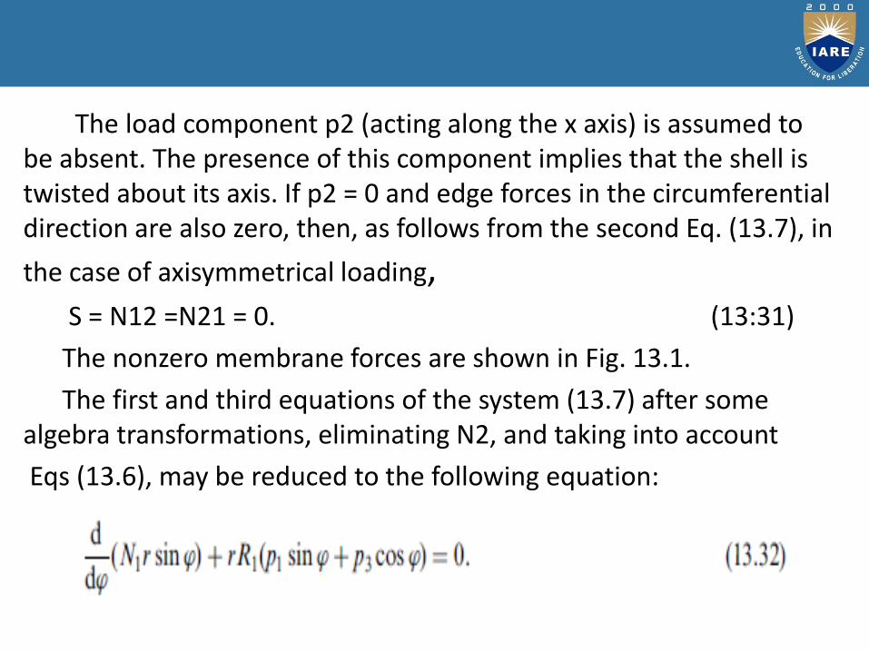
The load component p2 (acting along the x axis) is assumed to be absent. The presence of this component implies that the shell is twisted about its axis. If p2 = 0 and edge forces in the circumferential direction are also zero, then, as follows from the second Eq. (13.7), in

the case of axisymmetrical loading,S = N12 =N21 = 0. (13:31)

The nonzero membrane forces are shown in Fig. 13.1.

The first and third equations of the system (13.7) after some algebra transformations, eliminating N2, and taking into account

Eqs (13.6), may be reduced to the following equation:

UNIT – V

SHELLS OF REVOLUTION: WITH BENDING RESISTANCEE

As mentioned, shells of revolution belong to a highly generalclass of shells frequently used in engineering. One representativeof this class, cylindrical shells, was considered in Chapter 15, andwe will not dwell on these shells. The shell types analyzed in thischapter are subclasses of shells of revolution having non-zeroGaussian curvature. As mentioned in Sec. 11.7, such shells havenon-developable surfaces. Hence, they are stronger, stiffer, andmore stable than shells with zero Gaussian curvature. These shellsare frequently used to cover the roofs of sport halls and largeliquid storage tanks. The containment shield structures of nuclearpower plants also have dome-like roofs. Various pressure vesselsare either completely composed of a single rotational shell orhave shells of revolution at their end caps. Conical shells with zeroGaussian curvature are also representative of this class of shells:they are used to cover liquid storage tanks and the nose cones ofmissiles and rockets.

INTRODUCTION

In the membrane analysis of shells of revolution considered inearlier chapters, we saw that the membrane theory alone cannotaccommodate all the loads, support conditions, and geometries inactual shells. Thus, in a general case, shells of revolution experienceboth stretching and bending to resist an applied loading, whichdistinguishes significantly the bending of shells from the elementarybehavior of plates.

However, the character of bending deformation may bedifferent. If a shell of revolution is subjected to a concentrated force(Fig. 16.1a), bending exerts a crucial effect on its strength, because,in this case, the bending deformation increases with a growth of theforces until the load-carrying capacity of the shell structure isexhausted. In places of junction of a shell with its supports (Fig.16.1b) or other structural members (shell of another geometry, ringbeam, etc.), or in places of jump change in the radii of curvature (Fig.16.1c), the bending has another character; here, bending.

propagates only if it is needed to eliminate the discrepancies

between the membrane displacements or to satisfy theconditions of statics. If a shell material is ductile, the bendingdeformations of the latter type are usually decreased and do notpractically influence the load-carrying capacity of shell structures.If the material of the shell is brittle, the bending deformationsremain proportional to the applied loads until failure and canresult in a significant decrease in the strength of the shellstructure. In this chapter we consider the bending theory ofshells of revolution. It should be noted that the solutions of thegoverning differential equations involve many difficulties for ageneral shell of revolution, and therefore, we solve theseequations for some particular shell geometries and loadconfigurations that are frequently used in engineering practice.

Dead loads are those that are constant in magnitude andfixed in location throughout the lifetime of the structure suchas: floor fill, finish floor, and plastered ceiling for buildings andwearing surface, sidewalks, and curbing for bridges

Live Loads

Live loads are those that are either fully or partially in placeor not present at all, may also change in location; the minimumlive loads for which the floors and roof of a building should bedesigned are usually specified in building code that governs at thesite of construction (see Table1 - “Minimum Design Loads forBuildings and Other Structure.”)

Environmental Loads

Environmental Loads consist of wind, earthquake, and snowloads. such as wind, earthquake, and snow loads.

Serviceability

Serviceability requires that

• Deflections be adequately small. • Cracks if any be kept to atolerable limits. • Vibrations be minimized

We present below the governing differential equations ofthe moment theory of shells of revolution of an arbitrary shape.As curvilinear coordinates and of a point on the shell middlesurface, it is convenient to take the spherical coordinates,introducedin Sec. 11.8, and used in the membrane theory ofshells of revolution in Chapters 13and 14. Thus, we take ¼ ’ and¼ . As before, the angle ’ defines the location ofa point along themeridian, whereas characterizes the location of a point alongthe parallel circle (see Fig. 11.12). Let R1 and R2 be the principalradii of curvature of the meridian and parallel circle,respectively. Obviously, R1 and R2 will be functions of ’ only, i.e.,R1 ¼ R1ð’Þ and R2 ¼ R2ð’Þ. The Lame´ parameters in this caseare determined by the following formulas (see Sec.11.8):

GOVERNING EQUATIONS

The Codazzi and Gauss conditions are given by Eqs (11.41).

Let us consider the kinematic relations of the momenttheory of shells of revolution. Displacement components of themiddle surface along the given coordinate axes are u (in themeridional direction), v (in the circumferential direction), and w(in the normal direction to the middle surface). The strain–displacement relations (12.23) and (12.24) of the general shelltheory – taking into account Eqs (16.1) and (11.41) – take thefollowing form for shells of revolution:

Network models have three main advantages over linear

programming:

1.They can be solved very quickly. Problems whose linearprogram would have 1000 rows and 30,000 columns can besolved in a matter of seconds. This allows network models to beused in many applications (such as real-time decision making)for which linear programming would be inappropriate.

2. They have naturally integer solutions. By recognizing that aproblem can be formulated as a network program, it is possibleto solve special types of integer programs without resorting tothe ineffective and time consuming integer programmingalgorithms.

3.They are intuitive. Network models provide a language fortalking about problems that is much more intuitive than the\variables, objective, and constraints" language of linear andinteger programming.

Quantitative analysis also helps individuals to make informedproduct-planning decisions. Let’s say a company is finding itchallenging to estimate the size and location of a new productionfacility. Quantitative analysis can be employed to assess differentproposals for costs, timing, and location. With effective productplanning and scheduling, companies will be more able to meettheir customers’ needs while also maximizing their profits.

Production Planning

Cost SlopeCost slope is the increase in cost per unit of time saved by

crashing. A linear cost curve is shown in Figure.

Linear Cost Curve

Cost slope=Crash cost Cc– Normal cost Nc/Normal time Ntt

Cost Slope in network analysis

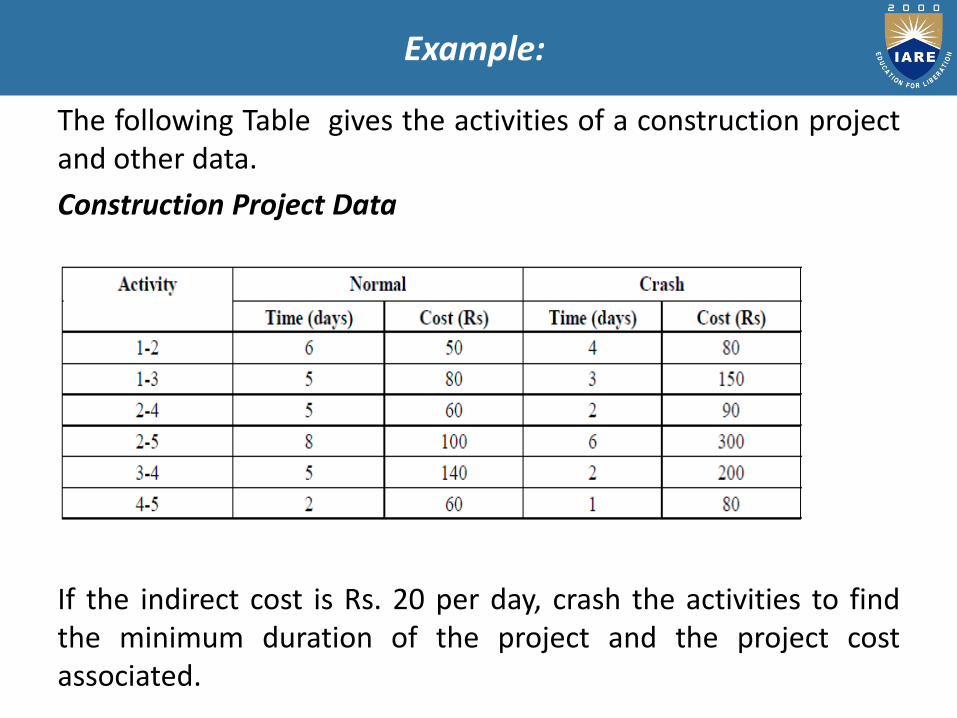
The following Table gives the activities of a construction projectand other data.

Construction Project Data

If the indirect cost is Rs. 20 per day, crash the activities to findthe minimum duration of the project and the project costassociated.

Example:

Solution: From the data provided in the table, draw the network diagram and find the critical path.

Network Diagram

From the diagram, we observe that the critical path is 1-2-5 with project duration of 14 days The cost slope for all activities and their rank is calculated as shown in table below

Cost slope=Crash cost Cc– Normal cost Nc/Normal time Ntt

Cost Slope for activity 1– 2 = 80 – 50/6 – 4 = 30/2 = 15.

The available paths of the network are listed down in Tableindicating the sequence of crashing.

Sequence of Crashing

Cost Slope and Rank Calculated

Network Diagram Indicating Sequence of Crashing

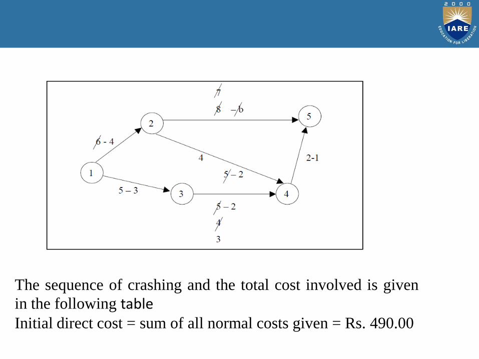
The sequence of crashing and the total cost involved is given

in the following tableInitial direct cost = sum of all normal costs given = Rs. 490.00

it is not possible to crash more than 10 days, as all the activities in the critical path are fully crashed. hence the project review techniques

Sequence of Crashing & Total Cost

The project review techniques are

In the critical path method, the time estimates are

assumed to be known with certainty. In certain projects likeresearch and development, new product introductions, it isdifficult to estimate the time of various activities. Hence PERT isused in such projects with a probabilistic method using threetime estimates for an activity, rather than a single estimate, asshown in Figure. Minimum project duration is 10 days with thetotal cost of Rs. 970.00.

Project review techniques

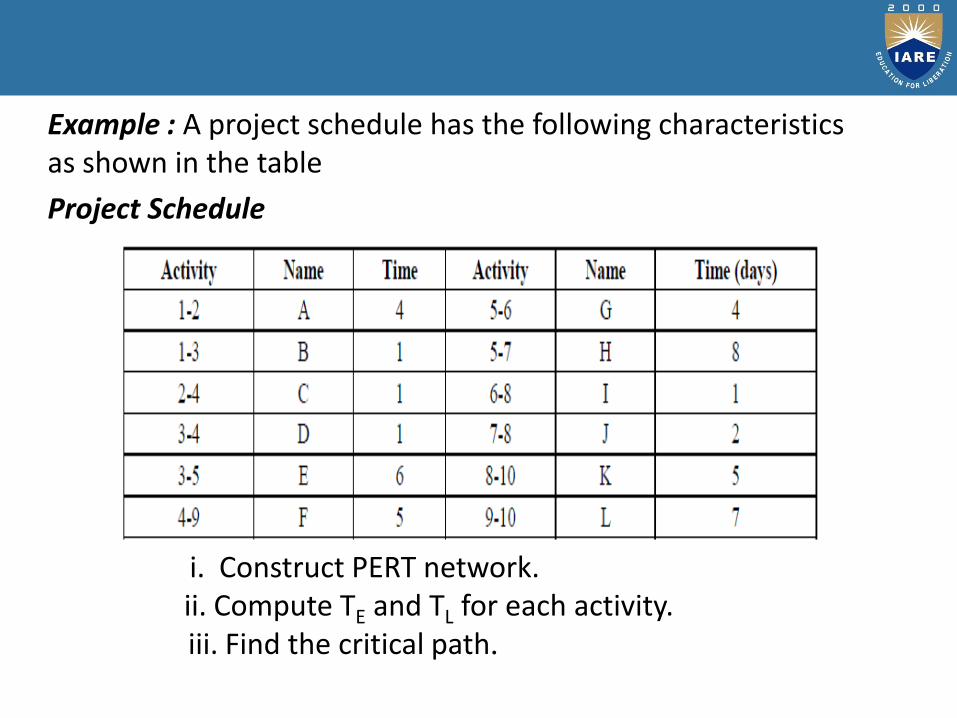
Example : A project schedule has the following characteristics as shown in the table

Project Schedule

i. Construct PERT network.ii. Compute TE and TL for each activity.iii. Find the critical path.

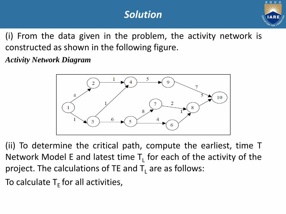
(i) From the data given in the problem, the activity network isconstructed as shown in the following figure.

Activity Network Diagram

(ii) To determine the critical path, compute the earliest, time TNetwork Model E and latest time TL for each of the activity of theproject. The calculations of TE and TL are as follows:

To calculate TE for all activities,

Solution

TE1 = 0TE2 = TE1 + t1, 2 = 0 + 4 = 4TE3 = TE1 + t1, 3 = 0 + 1 =1TE4 = max (TE2 + t2, 4 and TE3 + t3, 4)

= max (4 + 1 and 1 + 1) = max (5, 2)= 5 days

TE5 = TE3 + t 3, 6 = 1 + 6 = 7TE6 = TE5 + t 5, 6 = 7 + 4 = 11TE7 = TE5 + t5, 7 = 7 + 8 = 15TE8 = max (TE6 + t 6, 8 and TE7 + t7, 8)

= max (11 + 1 and 15 + 2) = max (12, 17)= 17 days

TE9 = TE4 + t4, 9 = 5 + 5 = 10TE10 = max (TE9 + t9, 10 and TE8 + t8, 10)

= max (10 + 7 and 17 + 5) = max (17, 22)= 22 days

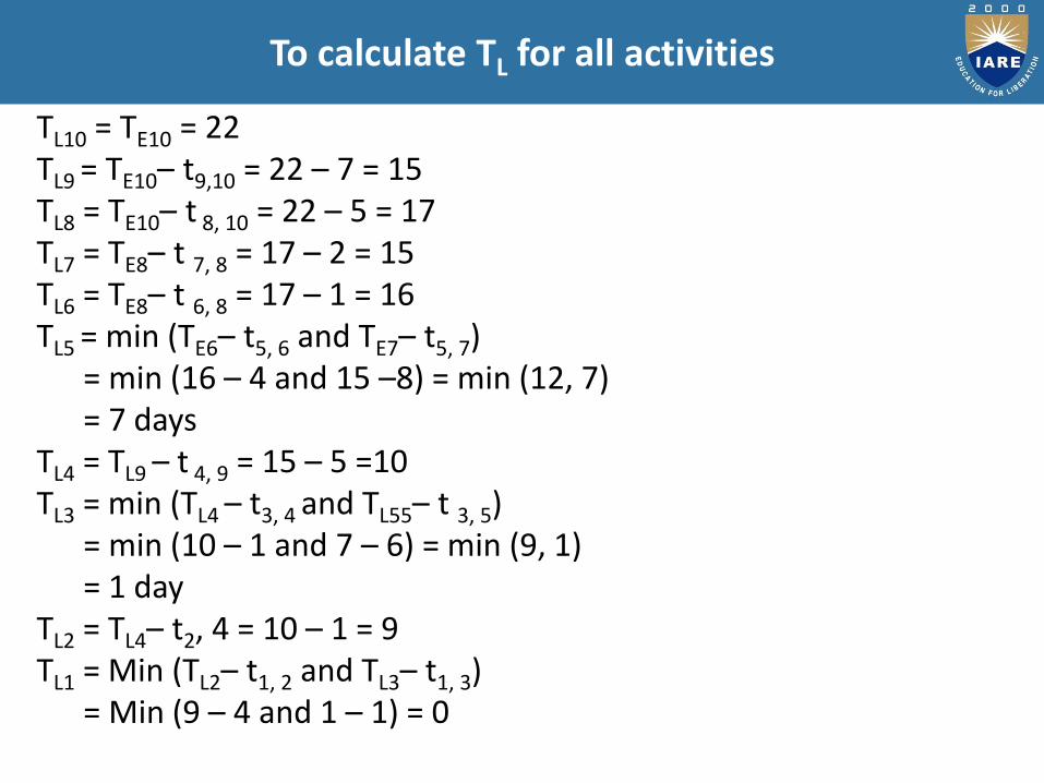
TL10 = TE10 = 22TL9 = TE10– t9,10 = 22 – 7 = 15TL8 = TE10– t 8, 10 = 22 – 5 = 17TL7 = TE8– t 7, 8 = 17 – 2 = 15TL6 = TE8– t 6, 8 = 17 – 1 = 16TL5 = min (TE6– t5, 6 and TE7– t5, 7)

= min (16 – 4 and 15 –8) = min (12, 7)= 7 days

TL4 = TL9 – t 4, 9 = 15 – 5 =10TL3 = min (TL4 – t3, 4 and TL55– t 3, 5)

= min (10 – 1 and 7 – 6) = min (9, 1)= 1 day

TL2 = TL4– t2, 4 = 10 – 1 = 9TL1 = Min (TL2– t1, 2 and TL3– t1, 3)

= Min (9 – 4 and 1 – 1) = 0

To calculate TL for all activities

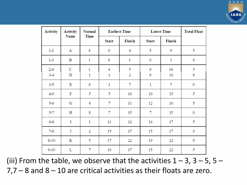
Various Activities and their Floats

(iii) From the table, we observe that the activities 1 – 3, 3 – 5, 5 –7,7 – 8 and 8 – 10 are critical activities as their floats are zero.

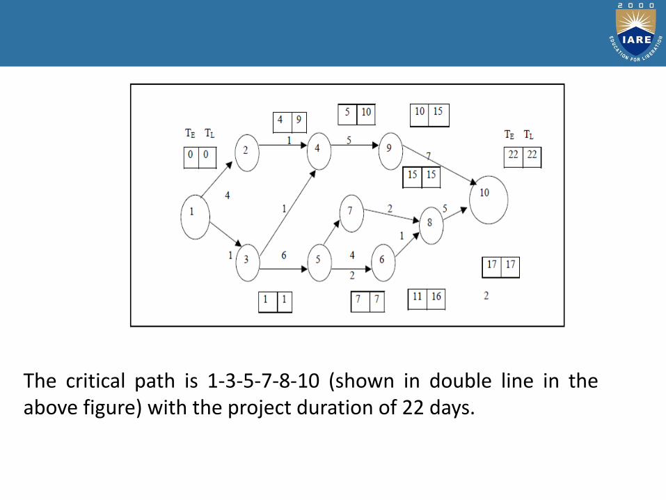
Critical Path of the Project

The critical path is 1-3-5-7-8-10 (shown in double line in theabove figure) with the project duration of 22 days.

PERT is an acronym for Program (Project) Evaluation andReview Technique, in which planning, scheduling, organizing,coordinating and controlling uncertain activities take place. Thetechnique studies and represents the tasks undertaken tocomplete a project, to identify the least time for completing a taskand the minimum time required to complete the whole project. Itwas developed in the late 1950s. It is aimed to reduce the timeand cost of the project.

PERT uses time as a variable which represents the plannedresource application along with performance specification. In thistechnique, first of all, the project is divided into activities andevents. After that proper sequence is ascertained, and a networkis constructed. After that time needed in each activity is calculatedand the critical path (longest path connecting all the events) isdetermined.

Pert

CPM

Developed in the late 1950s, Critical Path Method or CPM isan algorithm used for planning, scheduling, coordination andcontrol of activities in a project. Here, it is assumed that theactivity duration is fixed and certain. CPM is used to computethe earliest and latest possible start time for each activity.

The process differentiates the critical and non-criticalactivities to reduce the time and avoid the queue generation inthe process. The reason for the identification of criticalactivities is that, if any activity is delayed, it will cause thewhole process to suffer. That is why it is named as Critical PathMethod.

1.The most important differences between PERT and CPM areprovided below:

2.PERT is a project management technique, whereby planning,scheduling, organizing, coordinating and controlling uncertainactivities are done. CPM is a statistical technique of projectmanagement in which planning, scheduling, organizing,coordination and control of well-defined activities take place.

3.While PERT is evolved as a research and developmentproject, CPM evolved as a construction project.

4.PERT is set according to events while CPM is aligned towardsactivities.

5.A deterministic model is used in CPM. Conversely, PERT usesa probabilistic model.

Differences between PERT and CPM

9.PERT is used where the nature of the job is non-repetitive.In contrast to, CPM involves the job of repetitive nature.

6.There are three times estimates in PERT, i.e. optimistic time(to), most likely time ™, pessimistic time (tp). On the other hand,there is only one estimate in CPM.

7.PERT technique is best suited for a high precision timeestimate, whereas CPM is appropriate for a reasonable timeestimate.

8.PERT deals with unpredictable activities, but CPM deals withpredictable activities.

10.There is a demarcation between critical and non-criticalactivities in CPM, which is not in the case of PERT.

11.PERT is best for research and development projects, butCPM is for non-research projects like construction projects.

12.Crashing is a compression technique applied to CPM, toshorten the project duration, along with the least additionalcost. The crashing concept is not applicable to PERT.