Theory of the alternating-Gradient Synchrotronab-abp-rlc.web.cern.ch/ab-abp-rlc/AP-literature/Courant-Snyder... · In the alternating-gradient synchrotron the magnet ideally consists

Annals of Physics 281, 360�408 (2000)

Theory of the Alternating-Gradient Synchrotron1, 2

E. D. Courant and H. S. Snyder

Brookhaven National Laboratory, Upton, New York

Received July 15, 1957

The equations of motion of the particles in a synchrotron in which the field gradient index

n=&(r�B) �B��r

varies along the equilibrium orbit are examined on the basis of the linear approximation. Itis shown that if n alternates rapidly between large positive and large negative values, thestability of both radial and vertical oscillations can be greatly increased compared to conven-tional accelerators in which n is azimuthally constant and must lie between 0 and 1. Thusaperture requirements are reduced. For practical designs, the improvement is limited by theeffects of constructional errors; these lead to resonance excitation of oscillations and conse-quent instability if 2&x or 2&z or &x+&z is integral, where &x and &z are the frequencies ofhorizontal and vertical betatron oscillations, measured in units of the frequency of revolution.

The mechanism of phase stability is essentially the same as in a conventional synchrotron,but the radial amplitude of synchrotron oscillations is reduced substantially. Furthermore, ata ``transition energy'' E1 r&xMc2 the stable and unstable equilibrium phases exchange roles,necessitating a jump in the phase of the radiofrequency accelerating voltage. Calculationsindicate that the manner in which this jump is performed is not very critical. � 1958 Academic

Press

1. INTRODUCTION

The particles in a circular magnetic accelerator, such as a synchrotron, cyclotron,or betatron, are confined to the vicinity of their equilibrium orbit by magneticfocusing forces. These forces are conventionally obtained by shaping the magneticfield in such a way that

0<n<1, (1.1)

doi:10.1006�aphy.2000.6012, available online at http:��www.idealibrary.com on

3600003-4916�58 �35.00Copyright � 1958 by Academic PressAll rights of reproduction in any form reserved.

Reprinted from Volume 3, pages 1�48.1 This paper is a revised version of a report written by us in 1953 and privately circulated at that time.

Many if not most of the results obtained here have also been obtained independently by numerous otherauthors, especially members of the accelerator design groups at CERN, Geneva; Saclay, France; Harwell,England; and Cambridge, Massachusetts. No attempt has been made here to allocate credit for everysingle result. Comprehensive accounts of the theory of betatron oscillations, using somewhat differentapproaches from ours, may be found in references 9, 13, and 14.

2 Work done under the auspices of the U. S. Atomic Energy Commission.

where

n=&(r�B)(�B��r) (1.2)

is the field gradient index. Increasing n strengthens the vertical focusing forces at theexpense of the radial, while decreasing n has the opposite effect; the inequalities(1.1) impose limits on the strength of both focusing forces.

It has been shown [1, 2] that these limitations on the strength of the focusingforces can be overcome by letting the field gradient vary azimuthally, that is, byabandoning the axial symmetry that has characterized the fields of accelerators inthe past (straight sections in some synchrotrons, of course, also represent somedeviation from axial symmetry, but this has been more a perturbation than anessential feature). It was shown in reference [2] (hereafter referred to as CLS) thatby letting n in (1.2) alternate between large positive and large negative values atsuitable azimuthal intervals, one can obtain focusing forces an order of magnitudestronger than in an accelerator in which (1.1) is satisfied.

In the present paper we shall examine the characteristics of synchrotrons incor-porating this ``strong-focusing'' or `àlternating-gradient'' scheme in more detail thanwas given in CLS. We are concerned with oscillations of two types: ``betatron''oscillations, whose behavior is governed by the properties of the guide field andwhich are independent of the accelerating field, and ``synchrotron'' oscillations arisingfrom the acceleration process. Considering these problems separately is justified [3]as long as the frequency of betatron oscillations is large compared to that ofsynchrotron oscillations, which is the case here as well as in most existing syn-chrotrons.

2. STABILITY OF BETATRON OSCILLATIONS

The characteristics of betatron oscillations are essentially the same whether themagnetic fields are stationary or slowly varying with time. We shall thereforeassume in this and the following sections that we are dealing with stationarymagnetic fields. The effects of adiabatic variation of parameters will be discussed inSection 3d.

We consider a magnetic field B(r) which has the property that there is a planesuch that B at all points of the plane is perpendicular to the plane. This plane iscalled the median plane and is taken to be horizontal. (In Section 4c we shallabandon this condition of the existence of the median plane.) We further assumethat there is a closed curve in this plane such that a particle of a certain magneticrigidity p�e can move on this curve. We call this curve the equilibrium orbit.

In order to be usable as a guide field for accelerators, the magnetic field must besuch that the motion of a particle near the equilibrium orbit is stable in the follow-ing sense: if a particle, whose momentum is appropriate to the given equilibriumorbit, is started with a small intial displacement and a small initial angle from theequilibrium orbit, it will remain near the equilibrium orbit for all time.

361ALTERNATING-GRADIENT SYNCHROTRON

We characterize the position of a point P near the equilibrium orbit by thefollowing set of curvilinear coordinates:

s=the distance along the equilibrium orbit measured from some fixedreference point to that point on the orbit closest to the point P,

x=the horizontal component of the displacement of P from the equilibriumorbit (taken to be positive in the outward direction),

z=the vertical component of the displacement.

The motion of a particle near the orbit may be expressed in terms of s as the inde-pendent coordinate (see Appendix). If all terms of second and higher orders in x,z, and their derivatives are neglected, the equations of motion may be written in theform

d 2xds2 =&

1&n(s)\2(s)

x, (2.1)

d 2zds2 =&

n(s)\2(s)

z, (2.2)

where

\(s)= pc�eBz(s, 0, 0) (2.3)

is the radius of curvature of the equilibrium orbit at s, and

n(s)=&\(s)

Bz(s, 0, 0)�Bz(s, x, 0)

�x }x=0

=&\2

pc�e�Bz

�x(2.4)

is the field gradient at s.Since the equilibrium orbit is closed, the quantities n(s) and \(s) are periodic

functions of s, and (2.1) and (2.2) are examples of Hill's equation, i.e., linearequations with periodic coefficients and without first derivative terms. We writeboth equations in the form

d 2yds2 =&K(s) y, (2.5)

where y represents either horizontal or vertical displacement, and where K satisfiesthe periodicity relation

K(s+C)=K(s). (2.6)

Here C is the circumference of the equilibrium orbit.

362 COURANT AND SNYDER

In the alternating-gradient synchrotron the magnet ideally consists of N identicalsections or `ùnit cells,'' so that K also satisfies the stronger periodicity relation

K(s+L)=K(s); L=C�N. (2.7)

At this point it may be useful to review some of the properties of Hill's equation [4].The solution of any linear second order differential equation of the form (2.5),

whether or not K is periodic, is uniquely determined by the initial values of y andits derivative y$,

y(s)=ay(s0)+by$(s0),(2.8)

y$(s)=cy(s0)+dt$(s0),

or, in matrix notation,

Y(s)=_ Y(s)Y$(s)&=M(s | s0) Y(s0)=_a

cbd&_

y(s0)y$(s0)& . (2.9)

The usefulness of the matrix formulation (2.9) arises mainly from two features:In the first place, this formulation clearly separates the properties of the generalsolution of the problem from the features characterising any particular solution.That is, the matrix M(s | s0) depends only on the function K(s) between s0 and s, andnot on the particular solution. Secondly, the matrix for any interval made up ofsub-intervals is just the product, calculated by the usual rules of matrix multiplication,of the matrices for the sub-intervals, that is,

M(s2 | s0)=M(s2 | s1) M(s1 | s0), (2.10)

as is easily verified.The determinant of the matrix M is equal to unity, because the equation (2.5)

does not contain any first derivative terms.For the particular case of constant K the matrix takes the form

M(s0 | s)=_ cos ,&K1�2 sin ,

K&1�2 sin ,cos , & , (2.11)

where ,=K1�2(s&s0). If K is negative a more convenient way of writing this is

M=_ cosh �(&K)1�2 sinh �

(&K)&1�2 sinh �cosh � &, (2.12)

where �=(&K)1�2(s&s0). For an interval of length l in which K=0,

M=_10

l1& . (2.13)


For an interval in which K is piecewise constant the matrix is the product of theappropriate matrices of forms (2.11) to (2.13).

In the periodic systems we are considering here the matrices of particular interestare those which characterize the motion of the particle through a whole period. Wewrite

M(s)=M(s+L | s); (2.14)

this is the matrix for passage through one period, starting from s. Its elements areperiodic functions of s with period L. The matrix for passage through one revolu-tion is then

M(s+NL | s)=[M(s)]N,

and that for passage through k revolutions is [M(s)]Nk.In order for the motion to be stable as defined above, it is necessary and suf-

ficient that all the elements of the matrix MNk remain bounded as k increasesindefinitely. To obtain the condition for this, we consider the eigenvalues of thematrix M(s), that is, those numbers * for which the characteristic matrix equation

MY=*Y (2.15)

possesses nonvanishing solutions. The eigenvalues are the solutions of the deter-minantal equation

|M&*I|=0, (2.16)

or, more fully,

*2&*(a+d )+1=0, (2.17)

where we have made use of the fact that Det M=ad&bc=1. If we write

cos += 12 Tr M= 1

2 (a+d), (2.18)

the two solutions of (2.17) are

*=cos +\i sin +=e\i+. (2.19)

The quantity + will be real if |a+d |�2, and imaginary or complex if |a+d |>2.Let us now assume that |a+d |{2. Then the matrix M may be written in a form

which exhibits the eigenvalues and other properties explicitly. We define cos + by(2.18), and define :, ;, and # by

a&d=2: sin +,

b=; sin +, (2.20)

c=&# sin +;


the condition Det M=1 becomes

;#&:2=1. (2.21)

We resolve the ambiguity of the sign of sin + by requiring ; to be positive if|cos +|<1 and by requiring sin + to be positive imaginary if |cos +|>1. The defini-tion of + is still ambiguous to the extent that any multiple of 2? may be added to+ without changing the matrix. This ambiguity will be resolved later.

The matrix M may now be written as

M=_cos ++: sin +&# sin +

; sin +cos +&: sin +&=I cos ++J sin + (2.22)

where I is the unit matrix, and

J=_ :&#

;&:& (2.23)

is a matrix with zero trace and unit determinant, satisfying

J2=&I. (2.24)

It should be noted that the trace of M, and therefore +, is independent of thereference point s. For, by virtue of (2.10), we have for any s1 and s2

M(s2+L | s1)=M(s2) M(s2 | s1)=M(s2 | s1) M(s1), (2.25)

so that

M(s2)=M(s2 | s1) M(s1)[M(s2 | s1)]&1. (2.26)

Thus M(s1) and M(s2) are related by a similarity transformation, and thereforehave the same trace and the same eigenvalues. On the other hand, the matrix M(s)as a whole does depend on the reference point s. Thus the elements :, ;, # of thematrix J are functions of s, periodic with period L.

Because of (2.25), the combination I cos ++J sin + has properties similar tothose of the complex exponential ei+=cos ++i sin +; in particular, it is easily seenthat, for any +1 and +2

(I cos +1+J sin +1)(I cos +2+J sin +2)=I cos(+1++2)+J sin(+1++2). (2.27)

The kth power of the matrix M is thus

Mk=(I cos ++J sin +)k=I cos k++J sin k+, (2.28)

and the inverse is

M&1=I cos +&J sin +. (2.29)


It follows from (2.28) that if + is real the matrix elements of Mk do not increaseindefinitely with increasing k but rather oscillate; on the other hand, if + is not real,cos k+ and sin k+ increase exponentially, and therefore the matrix elements do thesame. Therefore the motion is stable if + is real, i.e., if |a+d |<2, and unstable if|a+d |>2.

In conventional circular accelerators, K(s) is constant, =n�R2 for vertical and(1&n)�R2 for horizontal oscillations, and L=2?R. Thus

+x=2?(1&n)1�2

+z=2?n1�2,

and the stability condition reduces to the well-known inequality (1.1). If Nequal straight sections of length l are introduced, the matrix for a unit cell is (2.11)multiplied by (2.13), and

cos +=cos ,&Nl,4?R

sin , (2.31)

as is well known [5].In alternating gradient synchrotrons [1, 2] the simplest magnet arrangement is

that of CLS:

\=const=R,

(2.32)n=n1 , 0<s<?RN

,

n=&n2 ,?RN

<s<2?R

N.

(The notation here is slightly different from that of CLS.)In this case the matrix for one period is the product of (2.11) and (2.12).

Computing its trace we find, for vertical oscillations,

cos +z=cos ,z cosh �z&n1&n2

2(n1 n2)1�2 sin ,z sinh �z , (2.33)

where

,z=?n1�2�N and �z=?n1�2�N,

and for horizontal oscillations,

cos +x=cos ,x cosh �x&2&n1+n2

[(n2+1)(n1&1)]1�2 sin ,x sinh �x , (2.34)


File: 595J 601208 . By:SD . Date:31:03:00 . Time:14:10 LOP8M. V8.B. Page 01:01Codes: 1488 Signs: 733 . Length: 46 pic 0 pts, 194 mm

FIG. 1. Region of stability for radial and vertical oscillations.

where

,x=?(n2+1)1�2�N and �x=?(n1&1)1�2�N.

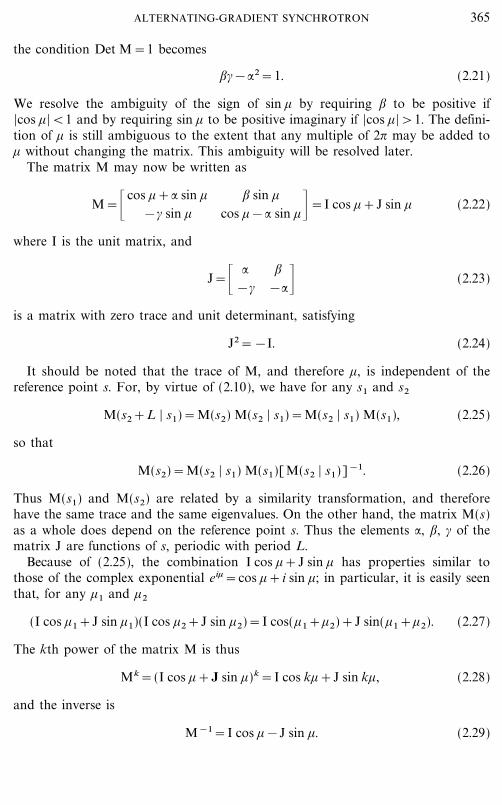
If n1>>1 and n2>>1, (2.34) is obtained from (2.33) by interchanging n1 and n2 ,and the stability criteria depend only on n1 �N2 and n2 �N2. Both modes are stableprovided n1�N 2 and n2 �N 2 lie within the ``necktie'' shaped region of Fig. 1.

3. AMPLITUDES OF BETATRON OSCILLATIONS

The motivation for proposing the alternating gradient configuration for themagnetic guide field in accelerators was the expectation that the effective focusingforces would be much stronger than in the corresponding conventional accelerators,leading to oscillations of smaller amplitudes around the equilibrium orbit, and


consequently smaller aperture requirements. In this section we shall first give thisstatement a precise meaning, and then investigate its validity quantitatively.

(a) Phase-Amplitude Form of the Solution

We may attempt to find solutions of Hill's equation (2.5) which have the form

y1(s)=w(s) ei�(s), (3.1)

where, for the moment, we impose no particular conditions on the functions w and�. It is easily verified by substitution that, if w and � satisfy

w"+Kw&1

w3=0 (3.2)

and

�$=1

w2 , (3.3)

then y1 as defined by (3.1) is indeed a solution, as is

y2(s)=w(s) e&i�(s), (3.4)

and that y1 and y2 are linearly independent. Therefore any solution of (2.5) is alinear combination of y1 and y2 . We can therefore write the matrix M(s2 | s1) interms of the solutions y1 and y2 or, what amounts to the same thing, in terms ofthe functions w and �. We obtain

M(s2 | s1)

=_w2

w1

cos �&w2w1$ sin �,

&1+w1w1$w2w2$

w1w2

sin �&\w1$w2

&w2$w1 + cos �,

w1w2 sin �

w1

w2

cos �+w1w2$ sin �& (3.5)

where � stands for �(s2)&�(s1), w1 for w(s1), etc.We now consider the case where s2&s1 is just one period of K(s), i.e., s2&s1=L.

The matrix M is then identical with the matrix (2.22).3 If we now require that w(s)be a periodic function of s, then w1=w2 and w1$=w2$ , and the forms (3.5) and(2.22) are identical provided we make the identifications

�(s2)&�(s1)=+ (3.6)

w2=;, (3.7)

ww$=&:, (3.8)


3 We again exclude the case were |cos +|=\1.

from which follows automatically

1+(ww$)2

w2 =1+:2

;=#. (3.9)

This identification is legitimate if we can show that ;1�2��which is, of course,periodic��satisfies the differential equation (3.2) and that

;$=&2:. (3.10)

To prove this, consider the matrix for the transformation from s+ds tos+L+ds. This matrix is, by (2.26),

M(s+ds)=M(s+ds | s) M(s)[M(s+ds | s)]&1. (3.11)

For infinitesimal ds,

M(s+ds | s)=_ 1&K(s) ds

ds1 & . (3.12)

Substituting (3.12) and (2.22) in (3.11) we find

M(s+ds)=M(s)+_(K;&#) sin +&2K: sin +

&2: sin +&(K;&#) sin +& ds, (3.13)

so that (3.10) is indeed valid, and furthermore

:$=&12

;"=K;&#=K;&1+:2

;(3.14)

and

#$=2K:. (3.15)

With the aid of (3.10) and (3.14) it is easily verified that ;1�2 does indeed satisfy(3.2), and is therefore a periodic solution of that equation. Now (3.7) and (3.8) arejustified, while (3.6) becomes the very important relation

+=|L

0

ds;

. (3.16)

(3.16) may be regarded as the definition of +. It is consistent with the previousdefinition (2.18), but has the advantage of being unambiguous, while (2.18) onlydefines + modulo 2?.


If we consider an accelerator of circumference C=NL with N identical unit cells,the phase change per revolution is, of course, N+. A useful number is

&=N+2?

=1

2? |s+C

s

ds;

; (3.17)

this is the number of betatron oscillation wavelengths in one revolution. (In theEuropean literature on accelerators this number is often denoted by Q.) A usefulinterpretation of & is as the frequency of betatron oscillations measured in units ofthe frequency of revolution; we shall generally refer to & simply as the frequency ofoscillations.

The two particular solutions y1 and y2 may now be written as

y12

=;1�2(s) e\i&,(s), (3.18)

where

,(s)=|ds&;

(3.19)

is a function which increases by 2? every revolution and whose derivative is peri-odic. The general solution of (2.5) is

y(s)=a;1�2 cos[&,(s)+$], (3.20)

where a and $ are arbitrary constants. This is a pseudo-harmonic oscillation withvarying amplitude ;1�2(s) and varying instantaneous wavelength

*=2?;(s). (3.21)

Incidentally, the relation (3.21) between the amplitude and the wavelength isformally just the same as in the WKB solution of the problem of the harmonicoscillator with varying wavelength; however, the relation between the wavelengthand the parameters of the differential equation is not as simple as in the WKBproblem.

In the treatment given here it has been tacitly assumed that ;(s) never vanishes,so that there are no singularities or ambiguities in the integral � ds�;. This is thecase when the motion is stable, i.e., when |cos +|<1. For then :, ;, and # are realand finite; it then follows from (2.21) that ; (and #) cannot vanish. In the unstablecase ( |cos +|>1, ; imaginary) the solutions can still be written in the form (3.18),but appropriate conventions have to be specified for integrating around the zerosof ;(s). On the boundary between stable and unstable regions ( |cos +|=1) thetreatment given here breaks down altogether. We do not propose to treat theunstable and boundary cases in detail here.


(b) Admittance

From the form (3.20) of the solution of the equation of motion it follows that thequantity

W=1;

[ y2+(:y+;y$)2]=#y2+2:yy$+;y$2 (3.22)

is constant, independent of s. Therefore the largest displacement is attained where; has its maximum value.

In a given accelerator, the motion is restricted by the walls of the vacuumchamber, or other obstructions, to a certain region around the equilibrium orbit, letus say to | y|<a. Then all particles whose initial conditions are such that

W<W0=a2

;max

will perform oscillations that remain within the vacuum chamber. FollowingSigurgeirsson [6], we define the admittance of the system as the area of that regionof ( y, y$) phase space for which any particles injected with initial values within theregion will remain within the vacuum chamber. This area is evidently the area ofthe ellipse (3.22), with W=W0 , that is,

A=admittance=?a2�;max . (3.23)

It is therefore desirable to design an accelerator with as small a value of ;max aspossible. The advantage of the alternating-gradient design is precisely that ;max canbe made smaller than in a conventional accelerator of the same radius.

From (3.19) we see that, if ;(s) were constant, it would be equal to

;� =C�2?&=R�&, (3.24)

where R=C�2? is the mean radius of the accelerator. In the general case, the maxi-mum value of ; will exceed ;� by some factor, which we call the ``form factor''

F=;max �;Av=&;max �R. (3.25)

The form factor F can generally be kept fairly small (say about 1.5), and thereforethe admittance of an alternating gradient machine is mainly governed by theoscillation frequency &.

In conventional accelerators &=n1�2 for vertical and (1&n)1�2 for horizontaloscillations; both these frequencies are less than 1. In alternating gradientaccelerators we can make & large, thus achieving a larger admittance for a givenaperture or alternatively a smaller aperture for a given admittance.

It follows from (3.20) that the maximum y at any particular s is proportional to;1�2. Therefore, if the vacuum chamber semiaperture a is constant all around the


machine, the particles will reach the walls only where ;=;max ; elsewhere they willonly attain a maximum amplitude

a(;�;max)1�2.

This makes it permissible to insert structures within the aperture of the vacuumchamber without reducing the space available to the beam��provided these struc-tures are placed where ;<;max and are close enough to the walls.

(c) Approximate Calculations

The general solution of Hill's equation

d 2yds2 +K(s) y=0 (2.5)

is characterized by the amplitude function

w(s)=;1�2(s), (3.26)

which is periodic in s with the same period C as K(s). We wish to find a methodfor obtaining ;(s) and

&=1

2? |C

0

ds;

(3.19)

approximately in the case where ;(s) does not fluctuate very much about its meanvalue.

Equations (3.12) to (3.14) can be combined to yield a single third-order differen-tial equation for ;:

;$$$+4K;$+2K$;=0. (3.27)

The amplitude function ;(s) is that particular solution of (3.27) which is periodicand is normalized so that

;#&:2= 12 ;;"& 1

4;$2+K;2=1. (3.28)

[Equation (3.28) has three linearly independent solutions; the other two are, ingeneral, the squares of the normal solutions of (2.5).]

We now write

K(s)= 12 =g(s) (3.29)

and

;=a[1+=f1(s)+=2f2(s)+ } } } ], (3.30)


that is, we regard the focusing function K(s) as ``small'' in some sense, and hope toobtain the deviation from constancy of the amplitude function ;(s) as a powerseries in the smallness parameter =.

Substituting in (3.27) we obtain the recursion relation

fn$$$=&2f $n&1g& fn&1g$, (3.31)

where we must impose the condition that fn is periodic and has zero mean value.It is not entirely obvious that this periodicity condition can be met. It is

necessary for this that the right hand side of (3.31) be a periodic function with zeromean. We can prove by induction that this is the case. For n=1, we have, from(3.31),

f1$$$=&g$. (3.32)

Since g$ is the derivative of a periodic function, it has zero mean, and therefore(3.32) can be solved for f1 . We may now write (3.32) in the form

fn$$$=&2( fn&1 g)$&( fn&1 f1)$$$+3( f $n&1 f1$)$+f $$$n&1 f1 (3.33)

so that the mean value is

( fn$$$) =+( f $$$n&1 f1). (3.34)

We now note that, for any r and s,

( fr$$$r fs) =( f $$$r&1 fs+1). (3.35)

This relation may be verified by using the recursion relation (3.31) for fr$$$ andintegrating by parts. Applying (3.35) to (3.34) n&2 times we find

( f $$$n&1 f1) =( f1$$$ fn&1). (3.36)

On the other hand, a straightforward triple partial integration yields

( f $$$n&1 f1) =&( f1$$$ fn&1). (3.37)

Therefore ( f $$$n&1 f1) =0, and (3.31) has a periodic solution.We now choose the normalizing constant so that (3.28) is satisfied. Thus, from

(3.19),

&2=1

8?2 \ ff "&12

f 2+=gf 2+_|C

0

dsf &

2

=1

16?2 (2=gf 2&3f 2)_|C

0

dsf &

2

. (3.38)


Expanding (3.38) in a power series in =, and making use of the relations satisfiedby the functions fn , we obtain

&2=C2

16?2 [2=g� +=2( f1$2) +=3(( f1$

2 f1)+ g� ( f 21) )+ } } } ]. (3.39)

Thus we have obtained the amplitude function and the frequency of oscillationin terms of integrals derived from the focusing function g(s). The procedure givenhere is particularly useful when = | f1 | is small, so that the amplitude function ;(s)is nearly constant.

Up to the second order in = our result is identical with that obtained from the``smooth approximation'' given by Symon [7]. It has the advantage that it is easyto see how to obtain higher approximations.

The first term in (3.39) is the focusing or defocusing effect of the mean restoringforce g� ; the second term shows that fluctuations about the mean value will alwaysproduce an additional focusing term. In alternating-gradient accelerators the firstterm is generally small or zero, and the focusing is mainly obtained from the secondterm.

As an example, consider the CLS configuration (2.32), with =g=2n�R2.In this case we obtain from the first two terms of (3.39)

&2=n1&n2

2+

?2

48(n1+n2)2

N2 . (3.40)

This is precisely what is obtained by expanding the left hand side of (2.33) in apower series in +z and the right hand side in a power series in n1 and n2 , ignoringterms of higher than second order in n1 and n2 or fourth order in +z , and notingthat &=N+�2?.

(d) Adiabatic Damping

As the particle is accelerated, its mass and velocity increase. Furthermore, theshape of the magnetic field may change (for example, because of saturation effects)and, therefore, its focusing properties will change. It is, therefore, desirable toinvestigate what happens to the amplitude of oscillations under these circumstances.

The effect of the increase in mass and velocity is the same as in conventionalcircular accelerations, namely, a damping of the amplitude proportional to p1�2,where p is the momentum of the particle [8]. The interesting question is: Whathappens when the focusing properties of the field change slowly, that is, when thematrix M changes slowly from one unit cell to the next?

Suppose we have

Yk+1=MkYk , (3.41)

Yk+2=Mk+1Yk+1=(Mk+=m) Yk+1 . (3.42)


We want to find an invariant, i.e., a quadratic form U whose coefficient matrix Vcan be calculated from the matrixes M and m, such that

Uk+1=Uk , (3.43)

except for terms of second and higher order in =. Here Vk+1 must be obtained fromthe elements of Mk+1 by the same prescription by which Vk is obtained from Mk .

Let us define, for any 2_2 matrix M, its ``conjugate''

M� =_ M22

&M21

&M12

M11 & . (3.44)

Then M+M� =Tr M and MM� =Det M; if M is unimodular, M� equals M&1.The invariant W [Eq. (3.22)] may be written

2W=1

sin +[X, V0Y ], (3.45)

where V0 is the matrix

V0=S(M&M� ) (3.46)

and

S=_01

&10 & . (3.47)

We, therefore, expect the adiabatic invariant to be of the form

Uk=[Yk , VkYk], (3.48)

with

Vk=ak[S(Mk&M� k)+=S(b&b� )],(3.49)

Vk+1=(ak+:=) S[Mk&M� k+=(m&m)+=(b&b� )].

The invariance condition Uk+1=Uk leads, if terms of order =2 are neglected, to

:(M&M� )+aM� (m&m� ) M+M� (b&b� ) M&(b&b� )=0, (3.50)

where we have left out the subscript k.The solution of (3.50) is

:a

=mM+M� m�

2&M2&M� 2=&2(sin +)

sin +, (3.51)


and

b=M� (Mm&mM)

4 sin2 +, (3.52)

where we have made use of the fact that both M and M+=m are unimodular and,therefore, mM� +Mm� =0.

It follows from (3.51) that the adiabatic invariant is

V=1

sin +S[M&M� +=(b&b� )]; (3.53)

this equals 2W as defined by (3.18) except for the small correction

=S(b&b� )�sin +.

Thus, to lowest order in =,

U=#y2+2:yy$+;y$2+=

2 sin +[Y, S(b&b� ) Y] (3.54)

is an adiabatic invariant as the focusing fields change slowly, and the amplitudeYmax varies approximately as ;max

1�2. Combining this result with the amplitudevariation proportional to p&1�2 arising from acceleration, we have the result: As theenergy and the focusing field change, the amplitude of oscillation varies as

(;max�p)1�2.

4. EFFECTS OF MAGNET IMPERFECTIONS

In an actual magnet the fields will differ somewhat from the ideal design. There-fore a particle which originally starts out on the ideal equilibrium orbit will, ingeneral, not stay exactly on that orbit but will deviate from it. The magnet is stillusable for an accelerator provided the following requirements are met at all timesduring the acceleration cycle:

(1) There exists a closed orbit, the ``displaced equilibrium orbit,'' which theparticle can follow, and which is located well within the aperture of the machine.

(2) Oscillations about this displaced equilibrium orbit are stable.

(a) Displacement of Equilibrium Orbits

Let y be the displacement��horizontal or vertical��from the ideal equilibriumorbit. Then the equation of motion of the particle is of the form

d 2yds2 +K(s) y=F(s), (4.1)


where we have neglected nonlinear terms, and where F(s) is a measure of the deviationof the field on the ideal orbit from its ideal value:

F(s)=2BB\

. (4.2)

Here B\ is the magnetic rigidity of the particle, and 2B=Br for vertical oscillationsand 2B=Bz&B0 for radial oscillations, both measured on the ideal orbit.

The inhomogeneous equation (4.1) may be solved in terms of the solutions of thehomogeneous equation (2.5), which are

;1�2 cos \| ds;

+$+=;1�2 cos(&,+$). (4.3)

We assume that the homogeneous solution is known, i.e., that we know thefunction ;(s).

We now introduce the new variables

'=;&1�2y, (4.4)

,=|ds&;

. (4.5)

Using the relations (3.12) to (3.14), the differential equation transforms to

d 2'd,2+&2'=&2;3�2F(s). (4.6)

The forcing term on the right hand side can be regarded as a function of the newindependent variable ,, periodic with period 2? in , corresponding to the periodC in s. We have thus reduced the problem of the forced oscillations of Hill'sequation to the forced oscillations of a harmonic oscillator.

The periodic solution of (4.6) is

'(,)=&

2 sin ?& |,+2?

,f (�) cos &(?+,&�) d�, (4.7)

where f (�)=;3�2F(s). Thus the displacement of the closed orbit becomes infinite (inthe linear approximation) when & is integral, i.e., when the perturbing force (whichis necessarily periodic with the period of the circumference) is in resonance with thefree betatron oscillations. Since small field deviations are unavoidable, the magnetmust be designed so that & is not integral for either mode.

Corresponding to the invariant W of Section 3 we have the quantity

V(,)='2+('�&)2=#y2+2:yy$+;y$2. (4.8)


From (4.7) we see that

V(,)=&2

4 sin2 ?& |,+2?

,|

,+2?

,f (�) f (/) cos &(�&/) d� d/. (4.9)

Another useful formulation of the problem is in terms of Fourier components.Let

f (,)=;3�2F(s)=:k

fke ik,, (4.10)

with

fk=1

2? |2?

0f (,) e&ik, d,=

12?& |

C

0;1�2F(s) e&ik, ds. (4.11)

Then the periodic solution of (4.6) is

'=:&2fk

&2&k2 eik,. (4.12)

This formulation clearly exhibits the resonance properties of the solution. We seethat the orbit is most sensitive to those Fourier components of the perturbationwhose order is close to the free oscillation frequency &, and that the Fouriercomponents must be taken with respect to the phase variable , rather than thegeometrical variable s.

In practice we usually do not know the perturbing function F(s) in detail, butknow some of its statistical characteristics. In that case we can make statisticalassertions about the equilibrium orbit. Consider, for example, a machine made ofM magnets, with a field error 2Br at the position of the ideal equilibrium orbit inthe r th magnet (assumed constant throughout that magnet). Let us define

2yr=Fr

Kr=

1B\

2Br

Kr, (4.13)

where we als assume that K(s)=Kr is constant in the magnet; furthermore weassume that all magnets have the same absolute value of K. The significance of 2yr

is that it is that displacement from the ideal position of the magnet which will justcause a field error 2Br , regardless of whether the error is actually caused by amagnet displacement or by an error in the intrinsic characteristics of the magnet.Assume further that the errors in different magnets are uncorrelated, and that themean square error is

(2y2)Av=$2. (4.14)


We now consider the expectation value of the amplitude of the displacedequilibrium orbit in an ensemble of machines having errors as described. Thequantity V defined by (4.9) is a convenient measure of the square of the amplitude.Its expectation value is

(V(,))Av=&2

4 sin2 ?& |,+2?

,|

,+2?

,( f (�) f (/)) cos &(�&/) d� d/. (4.15)

Since, by hypothesis, errors in different magnets are uncorrelated, ( f (�) f (/))=0unless � and / lie within the same magnet. Let us assume that the length of theindividual magnets is small compared to the wave length of betatron oscillations,i.e., small compared to ;. Then the factor cos &(�&/) can be replaced by unitywhen � and / are in the same magnet, f can be replaced by its value at the centerof the magnet, namely ;3�2K2y, and the interval of , corresponding to the magnetis L�&;, where L is the lenth of the magnet. Thus the contribution of the rth magnetto the double integral in (4.15) is

K2L2;r(2yr)2

&2 . (4.16)

The fluctuations in 2y from magnet to magnet are assumed uncorrelated; hence wemay averages ;r and 2yr

2 separately in averaging (4.16). The mean value of ;r isvery nearly R�& [see Eq. (3.24)]. The length of a magnet is 2?\�M, where \ is theradius of curvature in the magnets (\ is less than R if there are field-free sectionsbetween the magnets). Furthermore, K=\n�\2. Therefore

(V) Av=?2

sin2 ?&n2R

M&\2 $2. (4.17)

The amplitude of oscillations is given by Y=(;V)1�2. Again replacing ; by R�&, wefind for the mean square amplitude

(Y2) Av=?2

sin2 ?&R2

\2

n2

&2M$2. (4.18)

For the design of an accelerator it is desirable to have an estimate, not just of themean square amplitude, but of the largest amplitude that can reasonably be expec-ted. It has been shown by Lu� ders [9] that the higher moments of the distributionof Y2 satisfy

(Y2k) Av=k! [(Y 2)]k (4.19)

for k<<M. It follows that Y2 has an exponential distribution (corresponding to aRayleigh distribution in the amplitude Y). Thus the probability that Y2 exceeds


four times the mean value (4.18) is about e&4=0.02. It is thus safe to assume that,with 980 probability, the displacement of the closed orbit will be less than

P=2?

|sin ?&|R\

|n|&M1�2 F 1�2 (4.20)

times the root mean square equivalent displacement of the individual magnet,where F is the form factor defined by (3.25).

For the 30-Bev machine now under construction at Brookhaven, we haveR=421 ft, \=280 ft, |n|=360, M=240, =8.75, F 1�2=1.25, so that the multiplica-tion factor P equals 36. Thus if the errors in placement of the individual magnetsare random and uncorrelated with rms displacement of, say, 0.02 inch, the resultingequilibrium orbit is unlikely to deviate by more than 0.72 inch.

If we consider machines with different values of n and M but similar configura-tions of the unit period, we note that the phase shift + per period depends only onn�N2, and that &=N+�2? [Eq. (3.17)]. Let us assume that the parameters arevaried so as to keep n�N2 constant, and also so as to keep M�N (the number ofmagnets per unit cell) and \�R (the fraction of the circumference occupied bymagnets) constant. Also adjust n in each case so that sin ?& has the same value.Then n varies as N2, & varies as N, M varies as N, and F is constant; thus the factorP increases proportional to N1�2 or n1�4. This is in contrast with the amplitude fac-tor for free oscillations which, as we saw in Section 3, decreases with increasing n.

This leads to a fundamental limitation on the strength of focusing that is prac-ticable. The parameters of a machine have to be chosen so as to strike a com-promise between the decreased aperture requirements for free betatron oscillationsand the increased orbit deviations arising from errors in magnet placement. Thevery large values of n and & proposed in our original paper [2] appeared feasibleonly because at the time of writing that paper we were not sufficiently aware of theimportance of the effects of magnet errors.

(b) Errors in Field Gradients

The distribution of field gradients along the equilibrium orbit may also deviatefrom the ideal��due to variations in length of the individual magnet sectors, inmagnet gap dimensions, in iron properties, etc. As a result the periodicity condition

K(s+C�N)=K(s) (2.7)

is not exactly satisfied. However, the weaker periodicity relation

K(s+C)=K(s) (2.6)

remains valid. The stability and amplitude considerations of sections 2 and 3 stillapply, but the unit cell that must be considered is the whole revolution rather thanthe N th part of it, as in the ideal machine.


The matrix for the transformation about one revolution is still of the form (2.23).It may be written as the product of the individual��no longer quite identical��unitcell matrices

M= `N

i=1

Mi , (4.21)

where

Mi=I cos +i+Ji sin +i (4.22)

is the matrix for the i th unit cell.The stability condition is again

|Tr M|�2. (4.23)

In a perfect machine, Tr M=2 cos(N+), where + is the phase shift for one unit cell.If the imperfections are small, the matrix for the actual machine will differ onlyslightly from that for the perfect case; therefore the perturbations can cause (4.23)to be violated only if cos(N+) is near +1 or &1, that is, if &=N+�2? is near anintegral or half-integral value. Integral values of &, as we have seen, already lead todifficulties because of large deviations of the equilibrium orbit; thus the main practicaleffect of gradient errors is to introduce instability in the vicinity of half-integralvalues of &.

Another effect of the gradient errors will be to alter the amplitude function ;(s),and therefore the form factor F defined by (3.25) and the admittance of the system,even when stability is preserved.

To investigate these effects quantitatively, we write the equation of oscillationabout the actual equilibrium orbit in the form

d 2yds2 +[K0(s)+k(s)] y=0, (4.24)

where K0(s) is the focusing function for a perfect machine [satisfying the strongperiodicity relation (2.7)], and k(s) [satisfying only the weak periodicity relation(2.6)] is the perturbation. Suppose the solution for the perfect case (k=0) is knownand that the matrix for one complete revolution in the perfect case is

M0(s)=I cos +0+J(s) sin +0 ; J(s)=_ :(s)&#(s)

;(s)&:(s)& . (4.25)

Consider now a short interval of length ds1 near s1 . Its contribution to the matrixM0 is, in the limit K0

1�2 ds1<<1,

m0=_ 1&K0(s1) ds1

ds1

1 & , (4.26)


while its contribution to the actual matrix is

m=_ 1&[K0(s1)+k(s1)] ds1

ds1

1 & . (4.27)

If k were different from zero only in the interval ds1 , the actual matrix wouldbe obtained from M0(s) by replacing the contribution (4.26) by (4.27), that is, bymultiplying M0(s1) on the left by

mm0&1=_ 1

&k(s1) ds1

01& . (4.26)

Carrying out the multiplication, we find

Tr M=2 cos +=2 cos +0&(; sin +0) k(s1) ds1 . (4.29)

Thus the error k in the interval ds1 contributes &;(s1) k(s1) sin +0 } ds1 to the traceof the matrix. Adding the contributions from errors k(s) over the whole circum-ference we obtain

2(cos +)=&sin +0

2 |C

0;(s) k(s) ds, (4.30)

and the frequency shift is

2&=2+2?

=&2(cos +)2? sin +0

=1

4? |C

0;(s) k(s) ds. (4.31)

The expressions (4.30) and (4.31) are only first approximations, since terms ofsecond and higher orders in k are neglected. When sin +0 is near zero the secondorder approximation must be considered. If there is an error k(s1) ds1 near s1 andk(s2) ds2 near s2 , the matrix at s1 is

M(s1)=_ 1&k(s1) ds1

01& B _ 1

&k(s2) ds2

01& A, (4.32)

where A is the matrix of the unperturbed system from s1 to s2 , and B the matrixfrom s2 to s1+C. We may write

M(s1)=M0(s1)&(RBA) k(s1) ds1

&(BRA) k(s2) ds2+(RBRA) k(s1) k(s2) ds1 ds2 , (4.33)

where

R=_01

00& . (4.34)


The trace of M(s1) is

2 cos +=2 cos +0&(k1 ;1 ds1+k2 ;2 ds2) sin +0+B12A12 k1k2 ds1 ds2 , (4.35)

where we have written k1 for k(s1), etc.From (3.5) we obtain

A12=(;1 ;2)1�2 sin &(,2&,1),(4.36)

B12=(;1 ;2)1�2 sin &(2?&,2+,1)=(;1 ;2)1�2 sin[+0&&(,2&,1)].

Substituting in (4.35) and integrating, we find

cos +&cos +0=&sin +0

2 |C

0k(s) ;(s) ds

+12 |

C

0ds1 |

C

s1

ds2 k1k2;1 ;2 sin &(,2&,1) sin[+0&&(,2&,1)].

(4.37)

We are now in a position to find the width of a stopband, i.e., the width of thatrange of &=+0 �2? over which |cos +|>1. Consider the case where & is nearlyinteger,

&= p+=,

with p an integer and = small. Then, to second order in =,

sin +0=2?=; cos +0=1&2?2=2.

We neglect terms of higher than the second order in = and k combined. Therefore& in the arguments of the sines in the double integral in (5.37) may be replaced byp, +0 by 2?p, and the integral over the triangular region

|C

0ds1 |

C

s1

ds2

equals half the integral over the square region

|C

0ds1 |

C

0ds2 .

Writing the sine functions in terms of complex exponentials we obtain, after somemanipulation,

cos +&1=&2?2=2&?=J0+ 18 ( |J2p |2&J0

2), (4.38)


where, for any n,

Jn=|C

0;(s) k(s) e&in,(s) ds. (4.39)

Solving for cos +&1=0, we find

==&J0\|J2p |

4?(4.40)

so that the width of the stopband is

$&=|J2p |2?

=1

2? } |C

0;(s) k(s) e2ip,(s) ds } . (4.41)

The derivation for half-integral stopbands (&= p+ 12) is exactly analogous with the

result

$&=|J2p+1 |

2?. (4.42)

We may express these integrals in terms of the phase angle , as the independentvariable, with

ds=&; d,.

Thus

Jn=|2?

0&;2ke&in, d, (4.43)

is 2?& times the nth exponential Fourier component of ;2k, and the results of thissection are

shift of frequency [Eq. (4.31)]

2&= 12&(;2k)0 ; (4.44)

width of stopband

$&=&|(;2k)2& |. (4.45)

Beat Factors. The amplitude function ;(s) will also be modified by gradienterrors, and its maximum value, which determines the admittance of the system andalso the expected peak deviations of the closed orbit due to field errors, will ingeneral be larger in an imperfect machine than in a perfect one. Because theamplitudes of both free and forced oscillations, and hence aperture requirements,are proportional to ;1�2, it is desirable that the actual maximum value of ; exceedthe ideal maximum by as small a factor as possible.


We define the ``beat factor''

G=[;(actual)�;(ideal)]max (4.46)

for a machine in which the actual function ;(s) differs from the ideal one becauseof gradient errors.

To obtain the change in ; at some particular azimuth s1 we again consider firstthe contribution from the error k(s2) in an interval ds2 at s2 . This is obtained fromthe matrix (4.33) with k1=0:

M(s1)=M0(s1)=BRAk(s2) ds2

=M0(s1)&_B12A11

B22A11

B12 A12

B22 A12& k(s2) ds2 . (4.47)

The (12) element of M(s1), which is what determines ;, is, by (4.36),

M12(s1)=M120&B12A12k(s2) ds2

=;1 sin +0&;1;2 sin &(,2&,1) sin[+0&&(,2&,1)] k(s2) ds2 . (4.48)

Integrating over s2 , we obtain

2M12(s1)=&;1 |s1+C

s1

ds2 k2 ;2 sin &(,2&,1) sin[+0&&(,2&,1)].

But

2M12=2(; sin +)=2; sin +0+;1 cos +0 } 2+.

Using (4.31) we solve for 2;, obtaining

2;=;1

2 sin +0|

s1+C

s1

k(s2) ;(s2) cos 2&(?+,2&,1) ds2 (4.49)

=&;1

2 sin +0|

,1+2?

,1

k;2 cos 2&(?+,&,1) d,, (4.50)

where we have changed to the phase ,=� ds�&; as the independent variable. From(4.50) it is easily verified that the fractional change in ; satisfies the differentialequation

d 2

d,2

2;;

+4&2 2;;

=&2&2;2k(s), (4.51)


which is very similar in form to the equation (4.6) satisfied by the displaced equi-librium orbit, but with 2&, rather than & as the frequency of free oscillations. Wemay again solve (4.51) by Fourier analysis: we have

;2k(s)=1

2?&:�

p=&�

Jpeip,, (4.52)

where Jp is just the integral given by (4.30). Then the periodic solution of (4.51) is

2;;

=&&

4?:p

Jpe@p,

&2&( p�2)2 , (4.53)

which is, of course, equivalent to (4.50). The form (4.53) shows that the amplitudefunction is most sensitive to those harmonic components of the error in K(s), orrather in ;2K(s), whose order is nearest to 2&, and that it becomes infinite when 2&approaches an integer. If we consider only the leading term in (4.53), i.e., that valueof p which is closest to 2&, we have approximately

2;;

=&|Jp | cos( p,+$)

4?(&& p�2), (4.54)

where $ is a phase angle. Since the width of the stopband at &= p�2 is just |Jp |�2?[Eq. (4.41)], we see that the beat factor produced by the errors is related to thewidth of the nearest stopband produced by them,

G=1+(2;�;)max=1+($&)p

2(&&p�2), (4.55)

where ($&)p is the width of the stopband at p�2, and && p�2 is the distance from thestopband.

Effect of Random Errors. As an example, we again consider the form the fore-going effects take when the errors in n(s) or K(s) are randomly distributed inM magnets, with no correlation between the errors in different magnets. We havethe following root mean square ensemble averages for all orders p small comparedto M,

12?

( |Jp |) rms=1

2? �}� k;e&ip, ds }�rms

=M1�2 R\&M

krms=R |n|

\&M1�2 �2nn � rms

, (4.56)

where we have, in the averaging process, replaced ; by R�& and noted that theintegration is over M intervals of average lenth 2?\�M. For the machine now under


construction at Brookhaven (R=421 ft, \=280 ft, n=360, M=240, &=8.75) weobtain

12?

(Jp) rms=4.0(2n) rms .

The stopband width is just this, while the shift in & is J0�4?. The beat factor, for&=8.75, aries aqually from the stopbands at 17

2 and 182 , and is

G=1+4.0 �2nn � rms

.

Thus if the variation in n from magnet to magnet were 1 percent (rms), we would,on the average, expect &x and &z to differ from the design values by 0.02 unit, havestopbands of width 0.04 unit, and have a beat factor of 1.04. Any particularmachine might, of course, be worse than this, though it would be unlikely to beworse by more than factor of 2.

(c) Coupling between Horizontal and Vertical Oscillations

Up to this point we have assumed that horizontal and vertical deviations fromthe equilibrium orbit would be treated separately. This is the case when themagnetic field possesses a ``median plane,'' i.e., a plane on which the field iseverywhere perpendicular to the plane. However, the field of an actual magnet willdeviate slightly from this condition; consequently the equilibrium orbit need not bea plane curve, and the two types of oscillations may be coupled.

In this case it is convenient to make use of the Hamiltonian formulation of theequations of motion. It is shown in the Appendix that the equations of motion, withthe arc length s along the equilibrium orbit as the independent variable, can bederived from a Hamiltonian function

G(x, z, px , pz , s), (4.57)

which is periodic in s. Here x and z are the components of the displacement fromthe equilibrium orbit parallel and perpendicular to the oscillating plane, and px andpz are canonically conjugate momenta. The equations of motion are

x$=�G�px

, px$=&�G�x

,

(4.58)

z$=�G�pz

, pz$=&�G�z

,

where a prime, as usual, denotes differentiation by s.To obtain linear equations of motion we expand G as a power series in x, px , z,

pz and neglect all terms higher than the second order. Since x=z=0 is the equi-librium orbit, there are no first-order terms. Thus G is a homogeneous quadratic


function of x, px , z, pz . Because of Maxwell's equations it may be written in theform

G= 12 [K1x2+K2z2+2Mxz+( px&Qz)2+( pz+Qx)2]. (4.59)

In the particular case where the equilibrium orbit still lies in a plane, thesecoefficients have the following physical significance

K1=(1&n)

\2 , K2=n\2

as in the uncoupled case; M�K2 is the slope of the surface on which the field haszero radial component, and Q is proportional to the longitudinal or solenoidalcomponent of the magnetic field on the equilibrium orbit. If the equilibrium orbitis not plane, these interpretations must be modified slightly, but the Hamiltonianstill has the form (4.59).

When G is a quadratic form (regardless of whether it is of the particular form(4.59), or not), the equations of motion (4.58) are linear and therefore define alinear canonical transformation of (x, px , z, pz) phase space at s=s1 into phasespace at s=s2 . Such a transformation can, of course, be represented by a (4_4)matrix M,

X(s2)=M(s2 | s1) X(s1), (4.60)

where X(s) stands for the vector

_x(s)px(s)z(s)pz(s)& .

The Hamiltonian quadratic form G can also be represented by a��symmetrical��4_4 matrix: in vector notation

G= 12 [X, GX]. (4.61)

The equations of motion (4.58) then become, in matrix notation,

X$=SG X, (4.62)

where

S=_0100

&1000

0001

00

&10 & . (4.63)


It follows that, for any two solutions X1 and X2

dds

[X2 , SX1]=[X2$ , SX1]+[X2 , SX1$]=0, (4.64)

that is, the bilinear form

[X2 , SX1]=x1 px2&x2 px1+z1 pz2&z2 pz1

is invariant. Therefore, this form has the same value at s=s1 and at s=s2 . But, by(4.60),

[X2(s2), SX1(s2)]=[MX2(1), SMX1(s1)]

=[X2(s1) M� SMX1(s1)]=[X2(s1), SX1(s1)], (4.65)

where M� is the matrix obtained from M by transposing rows and columns. Sincethis relation is satisfied for any two solutions X1 and X2 the matrix M must satisfy

M� SM=S. (4.66)

This relation is due to Poincare� [10], who proved it for the matrix of partialderivatives �xi (s2)��xk(s1) for any canonical system, linear or not. Evidently, thetheorem holds for systems of any number k of dimensions, provided S is the(2k_2k) matrix obtained by writing

\01

&10 +

along the diagonal k times, and zero elsewhere.Matrices M satisfying (4.66) are said to be sympletic. From the symplectic

property of the transformation matrix we deduce that for each eigenvalue * of thematrix M, its reciprocal must also be an eigenvalue. For if we take for X1 and X2

the eigensolutions Xi and Xk of

MX=*X,

corresponding to the eigenvalues *i and *k , we have, from (4.65)

(*i*k&1)[X i (s1), SXk(s1)]=0. (4.67)

Given the eigenvector Xi , (4.67) must hold for all eigenvectors Xk . But thebilinear form [Xi , SXk] cannot vanish for all eigenvectors Xk , since any set ofinitial values is a linear combination of the four eigenvectors. Therefore at least oneof the eigenvalues is the reciprocal of *i . Therefore, the eigenvalues may bearranged in reciprocal pairs.



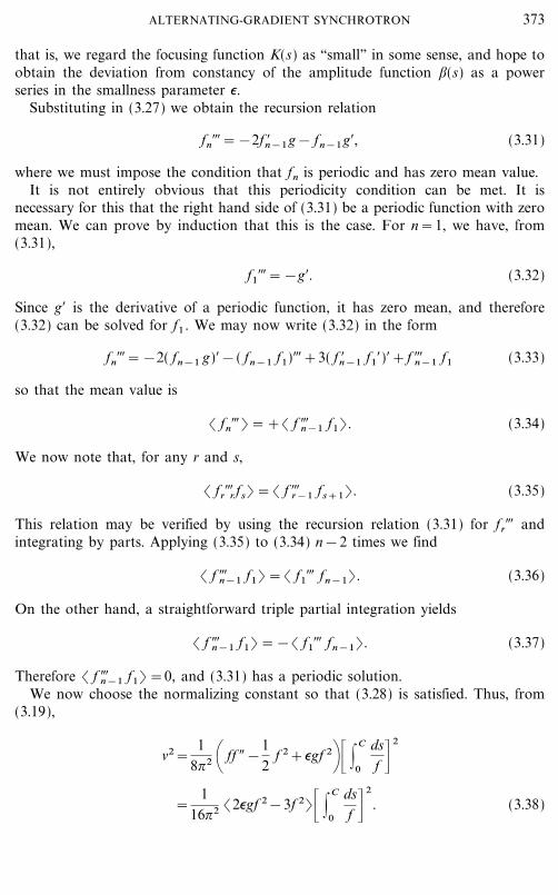
FIG. 2. Location of eigenvalues for two-dimensional linear oscillations. (a) Both modes stable. (b)One mode stable, one mode unstable. (c) Both modes unstable in absence of coupling. (d) Instabilityinduced by coupling.

It follows that the product of the eigenvalues, and therefore the determinant ofthe matrix M, is equal to unity (Liouville's theorem). However, the symplecticcondition is��for problems involving two or more degrees of freedom��a muchstronger restriction than just the conservation of volume in phase space. Liouville'stheorem imposes just one constraint on the (2k)4 elements of M (where k is thedimensionality of the problem), while the symplectic condition imposes k(2k&1)constraints [11]. Thus Liouville's theorem is equivalent to the symplectic conditiononly for one-dimensional systems.

Since M is real, the complex conjugate of an eigenvalue is also an eigenvalue. We thushave the following possibilities, assuming the eigenvalues to be distinct (Fig. 2):


4 Other proofs of this fact have been given by Lu� ders [12], Sturrock [13], and Seiden [14].

(a) All four eigenvalues lie on the unit circle, forming two complex conjugateand reciprocal pairs.

(b) One reciprocal pair is real, the others are complex and on the unit circle.

(c) Two real reciprocal pairs.

(d) One eigenvalue, say *1 , complex and not on the unit circle; the othereigenvalues must then be *2=1�*, *3=*1*, *4=1�*1*.

The motion is unstable if any eigenvalue is greater than 1 in absolute value. Thusonly situation (a) is stable. Cases (a), (b), and (c) correspond to the uncoupled casewith both modes stable, one mode stable and one unstable, and both modesunstable, respectively. Case (d) does not arise without coupling, and represents atype of instability that is generated only by the coupling.

We now ask: If the uncoupled motion is stable [case (a)], under what circurstancescan the coupling lead to instability?

We assume that the coupling is weak. Then the matrix with coupling differs onlyslightly from the unperturbed matrix, and the same is true of the eigevalues. Weexclude the case where the uncoupled system is near a resonance of the type wealready know to be harmful (& integral or half-integral, eigenvalues =\1). Thena small change in the eigenvalues cannot lead to situation (b) or (c), and it can leadto (d) only if the eigenvalues for the uncoupled modes are nearly equal, i.e., if,approximately,

cos +x=cos +z . (4.68)

Equation (4.68) means that either

&x+&z=integer (4.69)

or

&x&&z=integer. (4.70)

We shall now show that instability of type (d) cannot arise in case (4.70), but willin general arise in case (4.69)2.

We look for quadratic forms in the variables x, px , z, pz which are invariantunder the transformation (4.60), analogous to W [Eq. (3.21)] in the one-dimensional case. Such a quadratic form is given by a symmetrical matrix U whichmust satisfy

(X, UX )=(MX, UMX )=(X, M� UMX )

or

M� UM=U (4.71)


Using (4.66) we find that the matrix SU must commute with M. Therefore, thesymmetric solutions of (4.71) are

Uk=SMk&M� kS, (4.72)

where k is any integer; in general there are no other solutions except linearcombinations of the matrices Uk .

Now consider the uncoupled case, where

M=\0 0

+ ; (4.73)

A0 0

0 0D

0 0

A and D are the matrices of form (2.23) for the x and z motion, respectively. In thiscase it is easily seen that

[X, UkX]=2Wx sin k+x+2Wz sin k+z , (4.74)

where Wx and Wz are the invariants (3.18).The presence of coupling will add small terms to (4.74).When cos +x {cos +z , the invariance of (4.74) for all k implies that Wx and Wy

must be separately invariant. The only effect of coupling is to produce a slightchange in the forms Wx and Wz . On the other hand, when cos +x=cos +z , theneither sin k+x=sin 5+z for all k [case (4.70)] or sin k+x=&sin k+z [case (4.69)].Then the invariance (4.74) merely means that either

Wx+Wy

or

Wx&Wy

is invariant. In the former case, which corresponds to the difference &x&&y beingintegral, the invariant is positive definite, since Wx and Wy are separately positivedefinite. The addition of small terms arising from the coupling does not alter thepositive definite character. Therefore, the motion is bounded, and we have stability.

On the other hand, if &x+&y is integral, the invariant is the difference betweentwo positive definite quantities, and is therefore not definite. In that case, the couplingmay (and in general will) induce instability.


To demonstrate that instability does indeed occur, and to estimate how strong itis, we must compute the eigenvalues of the matrix M. We write M in the form

M=_AC

BD& , (4.75)

where A, B, C, D are 2_2 matrices. For any 2_2 matrix A we define its ``symplecticconjugate,'' as in (3.44),

A� =&_ 0&1

10& A� _ 0

&110&=_ A22

&A21

&A12

A11 & , (4.76)

and for a 4_4 matrix,

M� =&SM� S=_A�B�

C�D� & . (4.77)

The symplectic condition (4.66) then leads to

Det A+Det B=Det A+Det C=Det D+Det C=1 (4.78)

and

AC� +BD� =0. (4.79)

Since the eigenvalues of M come in reciprocal pairs, it suffices to find the twoquantities

2 cos +1=41=*1+1

*1

(4.80)

and

2 cos +2=42=*2+1

*2

. (4.81)

These are, of course, the eigenvalues of the matrix

M+M&1=M+M� =_A+A�C+B�

B+C�D+D� & . (4.82)

These eigenvalues satisfy the characteristic equation

42&4(A+A� +D+D� )+(A+A� )(D+D� )&(B+C� )(B� +C)=0, (4.83)


the solutions of which are

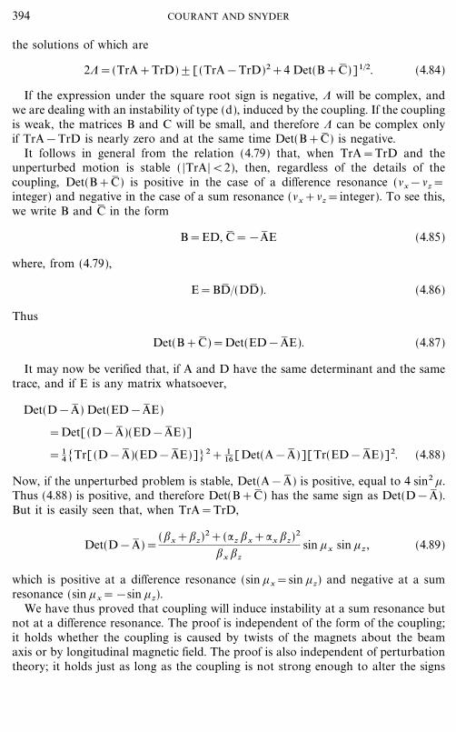
24=(TrA+TrD)\[(TrA&TrD)2+4 Det(B+C� )]1�2. (4.84)

If the expression under the square root sign is negative, 4 will be complex, andwe are dealing with an instability of type (d), induced by the coupling. If the couplingis weak, the matrices B and C will be small, and therefore 4 can be complex onlyif TrA&TrD is nearly zero and at the same time Det(B+C� ) is negative.

It follows in general from the relation (4.79) that, when TrA=TrD and theunperturbed motion is stable ( |TrA|<2), then, regardless of the details of thecoupling, Det(B+C� ) is positive in the case of a difference resonance (&x&&z=integer) and negative in the case of a sum resonance (&x+&z=integer). To see this,we write B and C� in the form

B=ED, C� =&A� E (4.85)

where, from (4.79),

E=BD� �(DD� ). (4.86)

Thus

Det(B+C� )=Det(ED&A� E). (4.87)

It may now be verified that, if A and D have the same determinant and the sametrace, and if E is any matrix whatsoever,

Det(D&A� ) Det(ED&A� E)

=Det[(D&A� )(ED&A� E)]

= 14 [Tr[(D&A� )(ED&A� E)]]2+ 1

16 [Det(A&A� )][Tr(ED&A� E)]2. (4.88)

Now, if the unperturbed problem is stable, Det(A&A� ) is positive, equal to 4 sin2 +.Thus (4.88) is positive, and therefore Det(B+C� ) has the same sign as Det(D&A� ).But it is easily seen that, when TrA=TrD,

Det(D&A� )=(;x+;z)

2+(:z ;x+:x ;z)2

;x ;zsin +x sin +z , (4.89)

which is positive at a difference resonance (sin +x=sin +z) and negative at a sumresonance (sin +x=&sin +z).

We have thus proved that coupling will induce instability at a sum resonance butnot at a difference resonance. The proof is independent of the form of the coupling;it holds whether the coupling is caused by twists of the magnets about the beamaxis or by longitudinal magnetic field. The proof is also independent of perturbationtheory; it holds just as long as the coupling is not strong enough to alter the signs


of Det(A&A� ) and Det(D&A� ). In these respects our proof is more general than theproofs given in refs. [12] and [14].

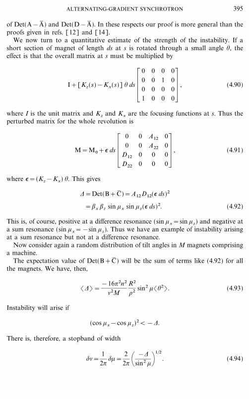
We now turn to a quantitative estimate of the strength of the instability. If ashort section of magnet of length ds at s is rotated through a small angle %, theeffect is that the overall matrix at s must be multiplied by

I+[Kz(s)&Kx(s)] % ds _0 0 0 00 0 1 00 0 0 01 0 0 0& , (4.90)

where I is the unit matrix and Kz and Kx are the focusing functions at s. Thus theperturbed matrix for the whole revolution is

M=M0+= ds _00

D12

D22

0000

A12

A22

00

0000& , (4.91)

where ==(Kz&Kx) %. This gives

2=Det(B+C� )=A12D12(= ds)2

=;x ;z sin +x sin +z(= ds)2. (4.92)

This is, of course, positive at a difference resonance (sin +x=sin +z) and negative ata sum resonance (sin +x=&sin +z). Thus we have an example of instability arisingat a sum resonance but not at a difference resonance.

Now consider again a random distribution of tilt angles in M magnets comprisinga machine.

The expectation value of Det(B+C� ) will be the sum of terms like (4.92) for allthe magnets. We have, then,

(2) =&16?2n2

&2MR2

\2 sin2 +(%2) . (4.93)

Instability will arise if

(cos +x&cos +z)2<&2.

There is, therefore, a stopband of width

$&=1

2?$+=

22? \

&2sin2 ++

1�2

. (4.94)


Its root mean square width is, by (4.93),

($&) rms=4 |n|

&M1�2

R\

(%) rms . (4.95)

For the Brookhaven parameters we obtain

($&) rms=16.0(%) rms .

Thus, if the rms tilt is 10&3 radian, we obtain an rms stopband width of 0.016 unit.

(d) Nonlinear Effects

The actual equations of motion will contain nonlinear terms as well. The detailedtheory of the effects of nonlinearities is beyond the scope of this paper, but thefollowing facts are worth mentioning.

Nonlinearities modify the behavior of the resonances we have just obtained fromthe linear theory. The shift of the equilibrium orbit, which is infinite accordingEq. (4.7) when & is integral, becomes finite, and the unstable oscillation arisingwhen & is half-integral or when &x+&z is integral also becomes limited in amplitude.Both these effects arise because the nonlinearity causes the frequency & to vary withamplitude; thus as the amplitude increases the frequencies change, and the resonantcondition ceases to apply.

On the other hand, nonlinearities can also cause instability in situations whichwould be stable in the linear theory. Specifically, instability can arise if

a&x+b&z=integer

with a and b integral [15]. However, it has been shown by Moser [16] andSturrock [17] that these instabilities will arise only if a and b are of the same sign,or if a or b is zero (analogous to the result in linear coupling resonance). Further-more, if a+b�5 the motion is generally stable even at resonance, because thedetuning effects of the nonlinearity dominate the resonance effects. For a+b=3,the system is generally unstable, while for a+b=4, the system may be stable orunstable depending on the relative magnitudes of certain coefficients; detailedcalculations show that it is more likely to be stable than unstable for practicalmachine designs. To summarize the effects of imperfections,

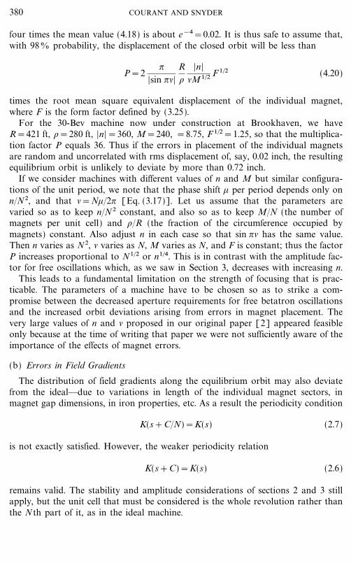
&x or &z=integer

imperfections will generally cause a large shift in the equilibrium orbit (infinite inthe linear approximation). If

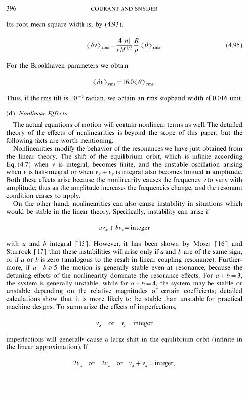
2&x or 2&z or &x+&z=integer,



FIG. 3. Values of &x and &z at which constructional errors may induce instability.

oscillations about the equilibrium orbit are in general unstable. Nonlinearitiesproduce further instabilities if

3&x or 2&x+&z or &x+2&z or 3&z=integer

and may also do so if

4&x or 3&x+&z or 2(&x+&z) or &x+3&z or 4&z=integer.

The values of &x and &z at which resonances may lead to instability are schemati-cally shown in Fig. 3.

5. PHASE STABILITY

The synchrotron [18, 19] is made possible by the phase stability of the acceleration,i.e., by the fact that a particle which arrives at the accelerating gap at a phase of


the accelerating field different from the equilibrium phase experiences a phaseacceleration or ``phase restoring force'' toward the equilibrium phase, provided thephase displacement and the momentum deviation of the particle are not too great.

Phase stability arises from the fact that the period of revolution of a particle withmore (or less) than the synchronous momentum differs from that of the particlewith the synchronous momentum. In the conventional synchrotron we have

2t�t=(2C�C )&(2v�v)=[(1&n)&1&(Mc2�E)2](2p�p), (5.1)

where 2t is the change in the period t of revolution, 2C is the change in the orbitcircumference C, and 2v is the change in the velocity v, associated with a change2p in the momentum p.

In the alternating gradient synchrotron the relation between orbit circumferenceand momentum is altered, so that the term (1&n)&1 in (5.1) must be replaced bya different quantity, depending on the field configuration. We shall see that thisquantity, the ``momentum compaction coefficients,''

:=2C�C2p�p

(5.2)

is small compared to unity in synchrotrons with strong alternating gradients. Then(5.1) is replaced by

2tt

=\:&E0

2

E 2 + 2pp

=\E02

E12 &

E02

E 2 + 2pp

='2pp

, (5.3)

where

E1=Mc2�:1�2 (5.4)

may be called the ``transition energy,'' and E0 is the rest energy.The coefficient ' of 2p�p in (5.3) is negative for energies less than E1 and changes

sign as the particle is accelerated through E1 . As pointed out in CLS, this meansthat at this point the equilibrium phase angle shifts from the rising to the fallingside of the voltage curve. To retain an accelerated beam beyond this energy it willbe necessary to shift the phase of the applied radiofrequency voltage by theappropriate amount at the proper time.

The equation of phase oscillation may be obtained from the two equations [3, 5, 20]

ddt \

2E|s +=

eV2?

(sin ,&sin ,0) (5.5a)

d,dt

&|1='h|s2pp

='h|s

;2

2EE

, (5.5b)


where the applied voltage is

V sin _| (h|s+|1) dt& ,

|s is the angular velocity of the particle, h the harmonic order (i.e., the appliedfrequency is designed to be h times the particle frequency), and |1 the frequency error,i.e., the difference between the actual applied frequency and its ideal value h|s .

Combining the two Eqs. (5.5) we find

1h|0

2

ddt _

E' \

d,dt

&|1+&=eV2?

(sin ,&sin ,0) (5.6)

where |0=|s �; is the circular frequency of a particle with velocity c. In theabsence of frequency errors Eq. (5.6) leads to stable small oscillations about thatphase at which sin ,=sin ,0 and ' cos ,0<0, while the other phase at whichsin ,=sin ,0 is a position of unstable equilibrium.

Just as in the case of the conventional synchrotron, the phase oscillations arestable for the range of phases from ?&,0 to that phase ,2 for which

cos ,2+,2 sin ,2=&cos ,0+(?&,0) sin ,0 . (5.7)

The amplitude of the associated radial oscillations may be obtained by using (5.2)and (5.5b). The amplitude of oscillations reaching to the limits of phase stability is

2rR

=: { eV?hp;c'

[(?&2,0) sin ,0&2 cos ,0]=1�2

. (5.8)

This differs from the expression for the conventional synchrotron in that it containsthe factor

:�|'|1�2 (5.9)

instead of

[(1&n)(1&(1&n) E02 �E 2)]&1�2. (5.10)

For nonrelativistic energies, 'r1, and (5.9) is very small compared to (5.10). There-fore the radial amplitude of synchrotron oscillations is greatly reduced in alternatinggradient synchrotrons as compared to conventional synchrotrons. In fact, thisreduction is so great that, for reasonable designs, the radial synchrotron oscillationamplitude is less than the betatron oscillation amplitude. This fact reduces thehorizontal aperture requirement to the point where it is not much greater than thevertical requirement��in contrast to large conventional synchrotrons such as theCosmotron at Brookhaven, which require horizontal apertures about five timestheir vertical apertures.


The small value of : does, however, introduce a complication. If the transitionenergy E1=E0 �:1�2 lies between the initial and final energies, ' changes sign as thetransition energy is passed, and the position of stable equilibrium jumps from ,0

(lying between 0 and ?�2) to ?&,0=,1 .Can the particles which were oscillating about ,0 before the transition be made

to oscillate stably about ,1 afterwards?Consider Eq. (5.6) before the transition and for small deviations in phase from

,0 . The equation becomes

ddt _

E&'

d,dt&+

h|02 eV cos ,0

2?(,&,0)=0. (5.11)

As long as ' varies slowly the solution is closely approximated by the adiabaticform

,&,0=A(&'�E )1�4 cos \| 0 dt+$+ , (5.12)

where

0=(&'heV cos ,0 �2?E )1�2 |0 (5.13)

is the circular frequency of synchrotron oscillations, and $ and A are constants.Thus the amplitude of phase oscillations damps down to zero as &' approacheszero. The concomitant radial oscillations are given, according to (5.5), by

2rr

=&A:; \e2V2 cos2 ,0

&'E 3h2 +1�4

sin \| 0 dt+$+ , (5.14)

so that their amplitude appears to become infinite as ' � 0. Actually this form orthe adiabatic approximation is, of course, not valid when ' approaches zero. Abetter procedure is to approximate '�E by a linear function of t in that region; thisleads to

,&,0=(&E0 �E )1�4 X 1�2[aJ2�3(X )+bN2�3(X )], (5.15)

with X=� 0 dt ; J2�3 and N2�3 are Bessel and Neumann functions of order 23 , and

a and b are constants. For large values of X this is identical with (5.12); for X � 0(5.15) approaches

,&,0 � &23�2b

31�3T( 13)

K, (5.16)

while the radial amplitude approaches

2rr

�23�2(31�2a&b) :

35�31( 53) K \heVE0 cos ,0

2?E12 +

1�2

, (5.17)


with

K=\2E07eV sin2 ,0

h?E18 cos ,0 +

1�12

. (5.18)

It is assumed here that the transition energy E1 is relativistic.The interesting quantities are the ratios of initial amplitudes to the amplitudes at

transition. These are, for the phase oscillations,

(,&,0)1

(,&,0) i=

2?1�2

31�31( 13) \

E i

E0'i+1�4

} K (5.19)

and for the radial oscillations

(2r�R)1

(2r�R) i=

4?1�2

35�21( 53)

; @ (E0Ei3' i)

1�4

E1 K. (5.20)

Numerically, for the parameters for the 30-Bev Brookhaven accelerator (injectionat 50 Mev, E1 r9Mc2, eV=190 kev, sin ,0= 1

2 , h=12), we find

(,&,0)1

(,&,0) i=0.103

(2p�p)1

(2p�p) i=0.42.

Thus at the transition energy the particles are very sharply bunched in phase; theirmomentum spread is fairly large but still relatively smaller than at injection, at leastin this numerical example.

This sharp bunching makes it possible to reestablish phase stability beyond E1 byshifting the phase of the applied rf at the time of transition. To see how this ispossible we multiply (5.6) by '2:

'*E

h|02 (,4 &|1)+

'h|0

2

ddt

[E(,4 &|1])&'2eV

2?(sin ,&sin ,0)=0. (5.21)

When ' is small the only important term is the first. Then the phase of the particlescan be shifted by simply shifting the phase of the rf by ,1&,0 , i.e., by introducinga perturbation |1 in the applied frequency for a time (,1&,0)�|1 .

The time during which this has to be done is not very critical, since the time con-stant for phase changes, i.e., the synchrotron oscillation period, is quite long. Thesecond and third terms of (5.21) will be small compared to the first as long as

|0'�'* |<1, (5.22)

which is the case when

|E&E1 |E1

<\ E1eV sin2 ,0

4?hE02 cos ,0+

1�3

. (5.23)


For our parameters this condition is |E&E1 |<124 Mev, which is satisfied duringapproximately 7 milliseconds.

This agrees with an expression found by Goldin and Koskarev [21].The quantity : which determines the transition energy is found as follows: When

the particle has momentum p+2p, we have

d 2xds2 +

(1&n)\2 x=

1\

2pp

. (5.24)

This is an inhomogeneous Hill's equation of the form studied in Section 4a. Wesolve it by the method of Fourier components used there: If

;3�2

\(s)=:

k

ak eik,(s), (5.25)

then the displaced equilibrium orbit is

x=2pp

;1�2&2 :k

akeik,

&2&k2 (5.26)

and, of course,

ak=1

2? |2?

0

;3�2

\e&ik, d,. (5.27)

The difference in length between this orbit and the original orbit x=0 is

2C=|C

0

x\

ds=& |2?

0

;x\

d,, (5.28)

where we use ,=� ds�&; as the variable of integration. Using (5.25) and (5.26), wefind

2C=2?&3 2pp

:k

|ak2|

&2&k2 (5.29)

and

:=1

2?R2C

2p�p=

&3

R:k

|ak2|

&2&k2 . (5.30)

In most accelerator designs, the dominant term in (5.25) and, therefore, in(5.30), is the one with k=0. If the magnet is composed of sectors in all of which


the radius of curvature \ is the same, separated by straight sections, we haveapproximately

a0=1

2? |2?

0

;3�2

\d,=

12?& |

C

0

;1�2

\dsr(R�&3)1�2, (5.31)

where we have replaced ; by its average value R�&.This leads to

:=1&2 (5.32)

and therefore,

E1=&E0 .

If the number of periods of the orbit is N, the only terms with k{0 in (5.30) willbe those with k=\N, \2N, etc. Since & will generally be less than N, all theterms with k>0 will then be negative. This fact has enabled Vladimirskii andTarasov [22] to propose an accelerator design in which : is zero or negative, thuseliminating the transition energy. This is done by inserting K ``compensatingmagnets'' with reversed fields but the same gradients as would be called for in adesign without compensating magnets. If & is slightly less than K, the term k=\Kin (5.30) is large and negative, and can be made to cancel the leading term k=0.

APPENDIX A: EXISTENCE OF EQUILIBRIUM ORBITS

Consider a magnetic field B in space. A particle of momentum p and electriccharge e moving in this field will move along a path whose curvature vector is

}=eB_:

pc, (A1)

where : is the unit vector in the direction of motion. If a closed curve satisfies (A1)throughout its length it is a possible equilibrium orbit for a particle of momentump; conversely any equilibrium orbit must satisfy (A1).

We shall now show that a curve which encloses the maximum flux as comparedto neighboring curves of the same circumference satisfies (A1) for a suitablemomentum, and is therefore a possible equilibrium orbit. Consider an arbitraryclosed curve of circumference C. Let s be the are length measured along this curve,and let its location be given by

r=r1(s) (A2)


Any other curve near the given one may be described by the equation

r=r2(s)=r1(s)+x(s), (A3)

where s is still the length of the first curve, and x(s) is a vector perpendicular to thefirst curve. The circumference of the curve (A3) is

C2=C+|C

0x } } ds, (A4)

where }(s) is the curvature vector of the first curve at s. If the second curve isrestricted to be a curve of the same length as the first,

|C

0x } } ds=0. (A5)

But the flux enclosed between the two curves is

28=|C

0B } :_x ds=|

C

0x } B_: ds. (A6)

If the original curve is an equilibrium orbit, (A1) holds, and therefore (A6)vanishes whenever (A5) does; hence the flux is stationary. Conversely, if the flux isstationary, (A6) must vanish whenever x(s) is chosen so that (A5) vanishes; there-fore a relation of the form (A1) must hold, and the curve is a possible equilibriumorbit. But a curve of given length enclosing maximum flux for all curves of thatlength will surely exist if the field strength is bounded. Hence equilibrium orbitsexist.

The maximum-flux orbits thus constructed will, in many cases, pass through thecurrents and iron which produce the magnetic field. The usable orbits will, ingeneral, enclose an amount of flux that is stationary but not maximal. The existenceof such orbits cannot necessarily be proved in the general case. However, in thespecial case of a field with mirror symmetry an equilibrium orbit may be found byconstraining the orbit to lie in the plane of symmetry. The curve of given lengthenclosing maximum flux subject to this constraint will be an equilibrium orbit andwill not intersect the iron or currents if these lie outside the plane of symmetry.

This result appears to be in contradiction to the result found in Section 4a, wherewe saw that when the oscillation frequency & is integral small imperfections of themagnetic field led to infinite displacements of the equilibrium orbit. However, thatresult was based on the linear approximation to the equations of motion; in anactual magnetic field the equations of motion are never exactly linear, and theactual displacement of the equilibrium orbit is always finite (though comparativelylarge when & is integral).


APPENDIX B: HAMILTONIAN FORMULATION OFTHE EQUATIONS OF MOTION

We suppose that the motion of the particle takes place in the vicinity of a givencurve in space��which may or may not be an equilibrium orbit as defined inAppendix A.

We introduce a special curvilinear system of coordinates in the vicinity of thisreference curve. Let the reference curve be given by

r=r0(s) (B1)

where s is the are length measured along the curve from some fixed initial point.Then

:(s)=dr0(s)

ds(B2)

is the unit vector tangent to the curve at s, and

}(s)=&d:(s)

ds=&0(s) ;(s) (B3)

is the curvature vector; 0(s) is the numerical value of the curvature and ;(s) is aunit vector. The plane containing the point r0(s) and parallel to : and ; is calledthe osculating plane; its unit normal is

#(s)=:(s)_;(s). (B4)

Since :, ;, and # are unit vectors, it is easily seen that

;$=0(s) :(s)+|(s) #(s),(B5)

#$=&|(s) ;(s),

where a prime denotes differentiation with respect to s, and where |(s) is a quantityknown as the torsion of the curve��for a plane curve, |(s) vanishes identically.

We now define the position of any point in space not too far from the referencecurve by

r(s, x, z)=r0(s)+x;(s)+z#(s), (B6)

where s, x, z form a system of orthogonal curvilinear coordinates. (B6) is uniquefor points whose distance from the reference curve is less than the radius ofcurvature \=1�0.


To express the equations of motion in Hamiltonian form in terms of these coor-dinates, we must find the momenta canonically conjugate to s, x, z. This is done byperforming a contact transformation produced by the generating function (23)

F ( pX , pY , pZ ; s, x, z)=p } [r0(s)+x;(s)+z#(s)], (B7)

where pX , pY , pZ are the components of the linear momentum p in the Cartesian(XYZ) coordinate system. We obtain the canonical momenta

ps=�F�s

=p } [(1+0x) :+|(x#&z;)],

px=�F�x

=p } ;, (B8)

pz=�F�z

=p } #.

The equations of motion are derived from the Hamiltonian

H=eV+c[m2c2+(p&eA)2]1�2, (B9)

where V and A are the scalar and vector potentials of the electromagnetic field. Interms of the new variables this equals

H=eV+c {m2c2+1

(1+0x)2 [ ps&eAs+|z( px&eAx)

&|x( pz&eAz)2+( px&eAx)2+( pz&eAz)2=

1�2

, (B10)

where As , Ax and Az are obtained by inserting the vector A in (B8) instead of p.Note that As and ps are not the components of the vectors in the tangential direction.

The Hamiltonian equations of motion are

s* =�H�ps

, p* s=&�H�s

,

x* =�H�px

, p* x=&�H�x

, (B11)

z* =�H�pz

, p* z=&�H�z

.


Using the first of these equations, we can change to s as the independent variableinstead of the time t. The equations transform to

x$= &�ps

�px, px$=

�ps

�x,

z$=&�ps

�pz, pz$=

�ps

�z, (B12)

t$=�ps

�H, H$=&

�ps

�t,

where primes denote differentiation with respect to s, and where ps is expressed asa function of x, px , z, pz , H, t, s, obtained by solving (B10).

Equations (B12) are again in Hamiltonian form, with the new Hamiltonian function

G=&ps (B13)

and the pairs of canonically conjugate variables

x, px ; z, pz ; t, &H. (B14)

In the particular case where the potentials V and A are independent of time,the new Hamiltonian G is also time-independent, and therefore t is an ignorablecoordinate in the system (B12). In this case the transformation just performedreduces the number of degrees of freedom of the problem from three to two, but atthe cost of having the new Hamiltonian dependent on the independent variable s.This procedure is important in classical dynamics [24, 25]. Because of the geometricalsignificance of the variable s, the dependence of the new Hamiltonian G on s isperiodic.

The linearized equations of motion are obtained by expanding G as a powerseries in x, px , z, pz and retaining only terms up to the second order. We considera static magnetic field, so that V=0 and A is independent of time. We may choosea gauge such that the power series expansions of the components of A are in theform

As=ax+bz+cx2+dx z+ez2+ } } } ,

Ax= & fz+ } } } , (B15)

Az=fx+ } } } .

Terms of higher order than those given in (B15) do not appear in the expansion ofG up to second order. The coefficients a, b, c, d, e, f, are periodic functions of s.

The only one of Maxwell's equations which imposes a restriction on thecoefficients up to this order is

({_B)s=({_{_A)s=0, (B16)


which leads to

2(c+e)=0a+4|f. (B17)

If the reference curve is taken to be an equilibrium orbit of a particle of momentump, we have

b=0, a=&0p�e. (B18)

In this case, by substituting (B15) in (B10) and (B12), we obtain a Hamiltonian Gof the form (4.59), and the homogeneous equations of motion used in Sections 2to 4.

REFERENCES

1. N. C. Christofilos, unpublished manuscript (1950).2. E. Courant, M. S. Livingston, and H. Snyder, Phys. Rev. 88 (1952), 1190.3. R. Q. Twiss and N. H. Frank, Rev. Sci. Instr. 20 (1949), 1.4. J. J. Stoker, ``Non-linear Vibrations,'' Chapter VI, Interscience, New York, 1950.5. N. M. Blachman and E. D. Courant, Rev. Sci. Instr. 20 (1949), 596.6. T. Sigurgeirsson, CERN Report CERN-T�TS�2 (unpublished, 1952).7. Symon, D. W. Kerst, Jones, Laslett, and Terwilliger, Phys. Rev. 103 (1956), 1837.8. D. W. Kerst and R. Serber, Phys. Rev. 60 (1941), 53.9. G. Lu� ders, Nuovo Cimento Suppl. 2 (1955), 1075.

10. H. Poincare� , ``Nouvelles Me� thodes de La Me� canique Celeste,'' Vol. 1, p. 193, Gauthier�Villars, Paris,1892.

11. H. Weyl, ``The Classical Groups,'' 2nd ed., Chapter VI, Princeton Univ. Press, Princeton, 1946.12. G. Lu� ders, ``Lectures, on the Theory and Design of an Alternating-Gradient Proton Synchrotron,''

p. 45, CERN, Geneva, 1953.13. P. A. Sturrock, ``Static and Dynamic Electron Optics,'' Chapter 7, Cambridge Univ. Press, London�

New York, 1955.14. J. Seiden, Ann. Phys. 10 (1955), 259.15. D. M. Dennison and T. H. Berlin, Phys. Rev. 69 (1946), 542.16. J. Moser, Nachr. Akad. Wiss. Go� ttingen IIa, No. 6 (1955), 87.17. P. A. Sturrock, Harwell Report AERE-X�R-1771, 1955 (unpublished) and Ann. Phys., to be pub-

lished.18. V. Veksler, J. Phys. USSR 9 (1945), 153.19. E. M. McMillan, Phys. Rev. 69 (1945), 143.20. D. Bohm and L. L. Foldy, Phys. Rev. 70 (1946), 249.21. L. L. Goldin and D. G. Koshkarev, Nuovo Cimento 2 (1955), 1251.22. V. V. Vladimirskii and E. K. Tarasov, ``Problems of Cyclic Accelerators,'' USSR Academy of Sciences,

Moscow, 1955.23. H. Goldstein, ``Classical Mechanics,'' Addison�Wesley, New York, 1953.24. E. T. Whittaker, `Ànalytical Dynamics,'' 4th ed., Chapter XII, Cambridge Univ. Press, London�New

York, 1937.25. G. D. Birkhoff, ``Dynamical Systems,'' Vol. 9, Chapter IV, American Mathematical Society

Colloquium Publication, New York, 1927.


Documents

Theory of the alternating-Gradient Synchrotronab-abp-rlc.web.cern.ch/ab-abp-rlc/AP-literature/Courant-Snyder... · In the alternating-gradient synchrotron the magnet ideally consists