Theory of large-scale matrix computation and applications ...coral.t.u-tokyo.ac.jp/hoshi/doc/2008_Fujiwara-arXiv_0802_0748.pdf · and applications to electronic structure calculation

Theory of large-scale matrix computationand applications to electronic structure calculation

T. Fujiwara1,2, T. Hoshi3,2 and S. Yamamoto2

(1) Center for Research and Development of Higher Education, The Universityof Tokyo, Bunkyo-ku, Tokyo, 113-8656, Japan(2) Core Research for Evolutional Science and Technology, Japan Science andTechnology Agency (CREST-JST), Japan(3) Department of Applied Mathematics and Physics, Tottori University, Tottori680-8550, Japan

Abstract. We review our recently developed methods for large-scale electronicstructure calculations, both in one-electron theory and many-electron theory.The method are based on the density matrix representation, together with theWannier state representation and the Krylov subspace method, in one-electrontheory of a-few-tens nm scale systems. The hybrid method of quantum mechanicalmolecular dynamical simulation is explained. The Krylov subspace method, theCG (conjugate gradient) method and the shifted-COCG (conjugate orthogonalconjugate gradient) method, can be applied to the investigation of the groundstate and the excitation spectra in many-electron theory. The mathematicalfoundation of the Krylov subspace method for large-scale matrix computationis focused and the key technique of the shifted-COCG method, e.g. the collinearresidual and seed switching, is explained. A wide variety of applications of theseextended novel algorithm is also explained. These are the fracture formation andpropagation, liquid carbon and formation process of gold nanowires, together withthe application to the extend Hubbard model.

PACS numbers: 61.46.-w,71.15.Dx,71.27.+a

Preprint (http://arXiv.org/abs/0802.0748v1) to appear in J. Phys. Cond. Mat. Contact URL; http://fujimac.t.u-tokyo.ac.jp/lses/index_e.html

Theory of large-scale matrix computationand applications to electronic structure calculation2

1. Introduction

Large-scale matrix computation is crucial in the electronic structure theory, bothin one-electron theory for large-scale systems and in many-body theory for stronglyinteracting electron systems. Interplay of the electronic structure and nano-scaleatomic structure plays an essential role in physical properties of nanostructurematerials and the Order-N algorithm has been extensively investigated. The sizeof the Hilbert space grows exponentially with linear increase of the system size inmany-electron problems.

Very important ten algorithms were invented in the 20th century. [1, 2] Thesealgorithms are the Krylov subspace method, the QR algorithm, the Householderalgorithm, the Fast Fourier Transformation (FFT) etc, where the most of them are ofthe matrix algebra and the order-N algorithm. The FFT algorithm is one of the basisof the local density approximation (LDA) in the density functional theory (DFT) andthe Lanczos method, one of the Krylov subspace method, is that of the many-bodyelectron theory. The efficiency of the modern Krylov subspace method seems not to bewidely known in the field of electron theory, both in LDA and many-electron theory.

In one-electron theory or DFT, the primarily important states are the statesnear the Fermi energy or the band gap. Then the standard mathematical tool isthe diagonalization of the Hamiltonian matrix. This may be a serious difficulty inlarge scale systems. In many electron theory, the difficulty is the huge size of theHamiltonian matrix and the resultant memory size and computational time. Theseare just the targets of the field of the large-scale matrix computation mentioned above.

In this paper, we report our recent activity in (1) developing thequantum mechanical molecular dynamical (MD) simulation method with the exactdiagonalization, the Wannier states representation and the Krylov subspace methodin nano-scale systems up to a few 10 nm size and (2) the investigation of many-electron problem, i.e. the degenerated orbital extended Hubbard Hamiltonian of thesize of 6.4 × 107, with the Krylov subspace method. We explain the key aspects inone-electron theory in a large-scale system and the many-electron theory in Sect. II.Section III is devoted to the explanation of the Krylov subspace methods. Severalapplications are reviewed in Sect. IV and the summary is given in the last section.

2. One-electron theory vs. many-electron theory

2.1. One-electron spectrum in large-scale systems

2.1.1. Density matrix formulationThe LDA calculation is based on the variational principles and usually on eigen-

function representation of the ground state. However, the eigen-functions are notalways necessary in actual calculation nor useful in numerical investigation of large-scale systems. Instead, one can construct the formulation with the one-body densitymatrix. [3] Any physical property can be represented by the density matrix ρ as

⟨X⟩ = Tr[ρX] =∑ij

ρijXij , (1)

where X is an operator of the physical property X and i and j denote atomic sitesand orbitals. Energy and forces acting on an individual atom can be calculated byreplacing X by the Hamiltonian or its derivative. Therefore, one needs only (i, j)



elements of the density matrix ρ corresponding to non-zero Xij but not all elements.The density matrix ρij is given as

ρ =(occ)∑

α

|φα⟩⟨φα|, (2)

where |φα⟩ is the eigenstates or the Wannier states and the summation is restrictedwithin the occupied states. It can be also written as

ρij = − 1π

∫ +∞

−∞dεImGij(ε)f

(ε − µ

kBT

), (3)

where Gij is the Green’s function defined as

Gij(ε) = [(ε + iδ − H)−1]ij . (4)Here, µ, kB, T and f are the chemical potential, the Boltzmann constant, thetemperature and the Fermi-Dirac distribution function, respectively.

We have developed a set of computational methods for electronic structurecalculations, i.e. the generalized Wannier-state method, [4, 5, 6] the Krylov subspacemethod (the subspace diagonalization method [7] and the shifted COCG method [8])and the generalized Wannier-state solver with parallelism. [9] These methods are onesfor calculating the one-body density matrix and/or the Green’s function for a givenHamiltonian. Calculation was carried out using the tight-binding formalism of theHamiltonian. These methods can be used in a hybrid way as is explained in 2.1.5. [10]

2.1.2. Wannier state representationThe Order-N algorithm can be constructed in semiconductors and insulators on

the basis of the Wannier state representation. The generalized Wannier states arelocalized wavefunctions in condensed matters obtained by the unitary transformationof occupied eigenstates, [11, 12, 4] and also obtained by an iterative way, starting atrial localize wavefunctions, with a mapped eigen-value equation [4]

H(i)WS|φ

(WS)i ⟩ = ε

(i)WS|φ

(WS)i ⟩, (5)

whereH

(i)WS ≡ H + 2ηsρi − Hρi − ρiH (6)

ρi ≡ ρ − |φ(WS)i ⟩⟨φ(WS)

i | =occ.∑

j(=i)

|φ(WS)j ⟩⟨φ(WS)

j |, (7)

and the energy parameter ηs should be much larger than the highest occupied level.Once one obtains the Wannier states, the density matrix can be easily constructedby Eq. (2) and the force acting on each atom can be calculated. We observed thatthe bond forming and breaking processes are well described in the localized Wannierstates as changes between a bonding and non-bonding orbital. The Wannier statesdepend upon the local environment and the above iterative procedure is suitable tothe MD simulation.

2.1.3. Krylov subspace methodIn metallic systems, the Krylov subspace method is very useful to achieve the

computational efficiency (accuracy and speed). [7, 8] The Green’s function can becalculated in the Krylov subspace and one calculates the density matrix by Eq. (3).Details are explained in Sec. 3. The Krylov subspace method is, of course, applicableto semiconductors and insulators, too.



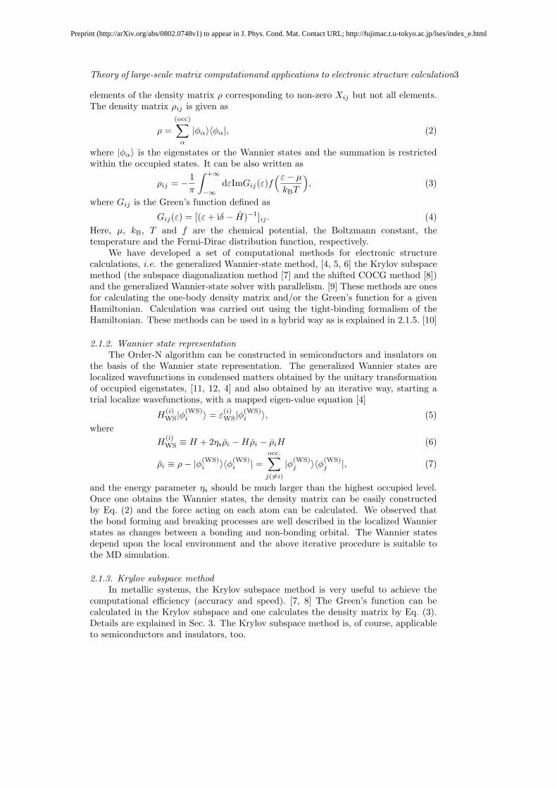
2.1.4. Comparison among solver methods and Order-N characterFigure 1 demonstrates our methods for 102-107 atoms with and without parallel

computation, [5, 6, 10] where the computational time is shown for the standardeigen-state solver (EIG) and our developed solver methods, Wannier-state solver withvariational procedure (WS-VR), Wannier-state solver with perturbation procedure(WS-PT) and Krylov subspace solver with subspace diagonalization (KR-SD). Parallelcomputations are achieved by the Open MP technique (http://www.openmp.org).The Hamiltonian forms used here are the Slater-Koster-form ones of silicon [13] andcarbon [14], the linear-muffin-tin orbital (LMTO) theory [15] in a form of the first-order (H(1)) for copper. Among the data in Fig. 1 except one by the eigen-state solver,the computational cost is ‘order-N ’ or linearly proportional to the system size (N), upto ten-million atoms and shows a satisfactory performance in parallel computation.The computational performance of the Wannier-state methods can be faster, at bestby several hundred times, than that of the Krylov subspace method (See Fig. 1, forexample), particularly, if a dominant part of wavefunctions are well localized. Nowthe program package (‘ELSES’ = Extra Large-Scale Electronic Structure calculation)is being prepared. [16]

Figure 1. The computational time as a function of the number of atoms (N).[5, 6, 10] The time was measured for metallic (fcc Cu and liquid C) and insulating(bulk Si) systems with up to 11,315,021 atoms, by the conventional eigenstatecalculation (EIG) and by our methods for large systems; KR-SD, WS-VR andWS-PT methods. See the original papers [5, 6, 10] for the details of parallelcomputation.

2.1.5. Multiple solver methodSince our method based on the density matrix formulation, we can construct

another very important method “the multiple solver method”. The basic idea is thedivision of the Hilbert space;

ρ = ρA + ρb, ρAρB = 0, (8)

and the calculation can be done independently on different parts A and B. Theimportance is the fact that this hybrid method is completely within the quantummechanical framework. Then we can use this hybrid scheme as the multiple solvermethod in nano-scale systems and the calculated results does not cause any artificial



discontinuity of physical quantities which might always occur in the hybrid schemeof naive simple division of the physical space. The choice or hybrid of the solversis important for an optimal calculation with a proper balance between accuracy andcomputational cost. [5, 10]

2.2. Ground state of many-electron theory and excitation spectra

In many-electron theory, we usually treat large matrices and the calculation becomesmore and more difficulty, since the occupation freedom of one site grows exponentiallyand the matrix size is extraordinarily large. [17] In order to get the precise eigen-energyand eigen-vector of the ground state, one should use the Lanczos method and the CGmethod (the inverse iteration method) simultaneously. The Lanczos method is usefulto get the approximate eigen-energy and eigen vectors of the ground state. However,the orthogonality of the generated basis vectors is broken at low iteration steps andthe precision of the ground state energy and wavefunction could not be preserved.Then we use the CG method (the inverse iteration method) to improve them. Afterestimating the accuracy of the calculation (the norm of residual vector), we shouldrepeat this procedure till the enough accuracy is obtained.

After we obtain the wavefunction of the ground state, we should analyze theproperties of excitations in a wide range of energy. For this purpose, the shiftproperty of the COCG method, i,e, the sifted COCG method, can be a powerfultool. The advantages of the shifted COCG method is an efficient algorithm of solvingshifted linear equations, the error-monitoring ability during the iterative calculationand the robustness. Then, it is very suitable for the problems in the many-electronproblem. [18] The detailed explanation is given in Sec.3.

3. Krylov subspace method

3.1. Krylov subspace

We consider the simultaneous linear equations

[(ε + iδ)1 − H] |xj⟩ = |j⟩, (9)

for a given vector |j⟩, real numbers ε and δ. 1 is the unit matrix. When H is a hugeN ×N matrix, the inverse of H or [(ε + iδ)1− H] is not easily obtained or impossibleto obtain and the iterative method becomes a useful concept. One can obtain anapproximate eigen vector |xj⟩ in a subspace spanned by vectors {Hn|j⟩};

Kν

(H, |j⟩

)≡ span

{|j⟩, H|j⟩, H2|j⟩, · · · , Hν−1|j⟩

}. (10)

This subspace Kν

(H, |j⟩

)is called the Krylov subspace. The basic theorem of the

Krylov subspace is the invariance of the subspace under a scalar shift σ1;

Kν

(H, |j⟩

)= Kν

(σ1 + H, |j⟩

). (11)

Lanczos found a new powerful way to generate an orthogonal basis for suchsubspace when the matrix is symmetric. [19] Hestenes and Stiefel proposed an elegantmethod, known as the conjugate gradient (CG) method, for systems that are bothsymmetric and positive definite. [20]



3.2. Subspace-diagonalization

The first method is to find eigen-vectors {|w(j)α ⟩} approximated in Kν

(H, |j⟩

)by

diagonalizing the reduced Hamiltonian matrix

HKν

(H,|j⟩

)= {⟨K(j)

n |H|K(j)m ⟩}, (12)

where {|K(j)m ⟩|m = 1, · · · , ν} is the orthogonalized basis set of the Krylov subspace

Kν

(H, |j⟩

), which satisfies the three-term recurrence relation and constructed by the

Lanczos process or the Gram-Schmidt process. In this subspace we can calculate thedensity matrix very easily. [7]

The subspace diagonalization method may be accurate enough for the severalpurposes in one-electron spectra in large-scale systems and calculation of total andlocal density of states. However, the orthogonality would be broken, when we use alarger number of the subspace dimension, for the basis vectors satisfying the three-termrecurrence relation. [7, 8] Therefore, the numerical accuracy may be limited when oneneed finer structure of spectra and we should extend the methodology to the shiftedCOCG method.

In many-electron theory, the Lanczos method is widely used for obtainingthe eigen-energy and many-electron wavefunction of the ground state in the exactdiagonalization method. The accuracy can be greatly improved when we use the CGmethod.

3.3. Shifted-COCG method and seed-switching technique

When the matrix (ε01 − H) is real symmetric, then one can use the CG method foran iterative solution of the simultaneous linear equation (ε01− H)x = b. One shouldintroduce the infinitesimal small (but finite) imaginary number iδ for the Green’sfunction and the matrix (ε0 + iδ)1 − H is complex symmetric. Then we can use theconjugate orthogonal conjugate gradient (COCG) method for solving the equation{(ε0 + iδ)1 − H}x = b. [8]

Since the energy parameters ε are arbitrary given or continuously changing in awide energy range, one should solve also the shifted linear equations

[(ε0 + σ + iδ)1 − H] |x(σ)j ⟩ = |j⟩, (13)

with a fixed energy (seed) ε0. The energy shift parameter σ can be even complex.The shifted-COCG method was constructed, [8, 18] in which the theorem of collinearresidual [21] for the shifted linear systems is applied to the COCG method. Theessential property is based on the basic invariance theorem of the Krylov subspaceEq. (11) under an energy shift ε0 + σ from ε0. Therefore, the Krylov subspacefor the equation [(ε0 + σ + iδ)1 − H] |x(σ)

j ⟩ = |j⟩ can be generated from that of[(ε0 + iδ)1 − H] |xj⟩ = |j⟩ of a selected seed energy ε0. The very important fact isthat this shift procedure is scalar linear calculation. Essential cost for solving Eq. (9)should be paid only for the seed energy ε0 and the rest is a scalar linear calculationwhich is negligible.

The choice of the seed energy is not unique and sometime the calculations cannotbe finished under a required criteria. Then one should continuously change the energyparameter and choose a new seed energy ε + iη again. Essentially important pointis that we can continue the calculation with a new seed energy, keeping calculatedinformation of the former seed energy. This is another very important property called‘seed-switching’. [22, 18]



3.4. Accuracy control with residual vector and robustness of shifted COCG method

It is essentially important to know the accuracy of the solution during the iterationprocedure and we can monitor the convergence behavior of the iterative solutions ofthe Krylov subspace method.

The residual vector can be defined both in the subspace diagonalization andshifted COCG method [8] as

|r(ν)j ⟩ = (ε + iδ − H)|x(ν)

j ⟩ − |j⟩, (14)

where |x(ν)j ⟩ is the ν-th iterative solution. This residual vector can be monitored during

the iterative calculation and we can stop the iterative procedure, without fixing thedimension of the Krylov subspace, once one can obtain the required accuracy. Thenorm of the residual vector can give the upper limit of the accuracy of the Green’sfunction itself. [18]

The shifted COCG method is numerically robust and one can reduce the normof the residual vector to the machine accuracy. Therefore, the shifted-COCG methodmay be used to calculate accurate or fine density of electronic states in one-electronspectrum in large-scale systems or the fine excitation spectra in many-electronproblems.

4. Applications

4.1. Application to nano-scale systems

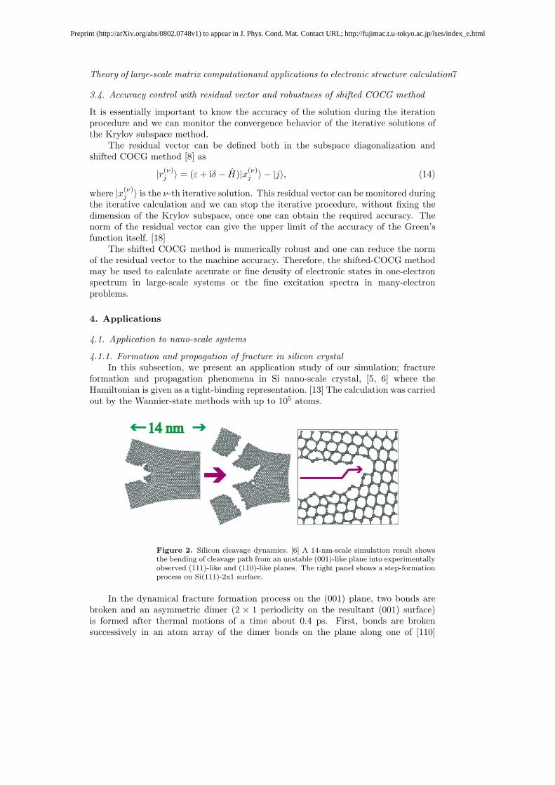
4.1.1. Formation and propagation of fracture in silicon crystalIn this subsection, we present an application study of our simulation; fracture

formation and propagation phenomena in Si nano-scale crystal, [5, 6] where theHamiltonian is given as a tight-binding representation. [13] The calculation was carriedout by the Wannier-state methods with up to 105 atoms.

Figure 2. Silicon cleavage dynamics. [6] A 14-nm-scale simulation result showsthe bending of cleavage path from an unstable (001)-like plane into experimentallyobserved (111)-like and (110)-like planes. The right panel shows a step-formationprocess on Si(111)-2x1 surface.

In the dynamical fracture formation process on the (001) plane, two bonds arebroken and an asymmetric dimer (2 × 1 periodicity on the resultant (001) surface)is formed after thermal motions of a time about 0.4 ps. First, bonds are brokensuccessively in an atom array of the dimer bonds on the plane along one of [110]



directions. Along the formed asymmetric dimer bonds, the inter-atomic distance isshortened due to the formed bonding bonds. The distortion energy is accumulatedand, then, other bonds along a parallel atom array, but not the same, are broken.This fracture propagation (perpendicular to the direction of the formed asymmetricdimer bonds) is governed by the accumulated distortion energy. Our calculation canrepresent this surface breaking mechanism on the (001) plane of Si crystals. [5]

We also studied with 14 nm scale Si crystals the easy-propagating plane offracture. [6] It is widely known that the easy-propagating plane of fracture in Si is(110) or (111) planes. In case of fracture on the (111) plane, the (111)-(2× 1) surfacereconstruction appears (the Pandy structure [23]) and several steps are formed. Thefracture propagation plane is not explained by the energy of established stable surfacesbut by that of ideal or transient surface structure without reconstruction. In a MDprocess in a larger systems with 14nm length, even if a fracture propagation startson a (001) plane, the plane of the fracture propagation changes to (111) and (110)planes. Figure 2 shows examples of the simulation results.

PC f

unct

ion

0

0.1

0.2

0.3

0.4

-30 -20 -10 0 10 20DO

S (1

/eV

/ato

m)

Distance

(a)

(b) KR:13824 atom

Figure 3. Molecular dynamical simulation of liquid carbon by the MD simulationwith the Krylov subspace method. (a) The pair correlation function and (b) theelectron density of states.

4.1.2. Liquid carbonLiquid carbon of 13,824 atoms was simulated with the Krylov subspace

method. [10] The density and the temperature are set to be ρ = 2.0 g cm3 andT = 6000 K. The time interval of a MD step is ∆t = 1 fs and the subspace dimensionand the number of interacting atoms are chosen to be ν = 30 and NPR = 200,respectively. Figure 3(a) shows the resultant pair correlation (PC) function withcomparison of the conventional eigenstate method of 216 atoms and we should noticethat the two graphs are identical. Figure 3(b) shows the electronic density of states(DOS) of a system of with 13, 824 atoms from the Greenfs function, by the Krylovsubspace method. The DOS calculation was achieved with the controlling parameters



of a heavier computational cost (ν = 300 and NPR = 1000) and η = 0.05 eV. Sincethe present Hamiltonian includes only s and p orbitals, the resultant DOS misses astructure in higher energy regions. The resultant DOS shows the characteristic profileof liquid carbon, e.g. a narrow π band appears between −5 and +5 eV as in carbonnanotubes. The π bond in the liquid phase is imperfect and non-bonding (atomic) pstates appear as a sharp peak near the chemical potential (ε ≅ 0.6 eV).

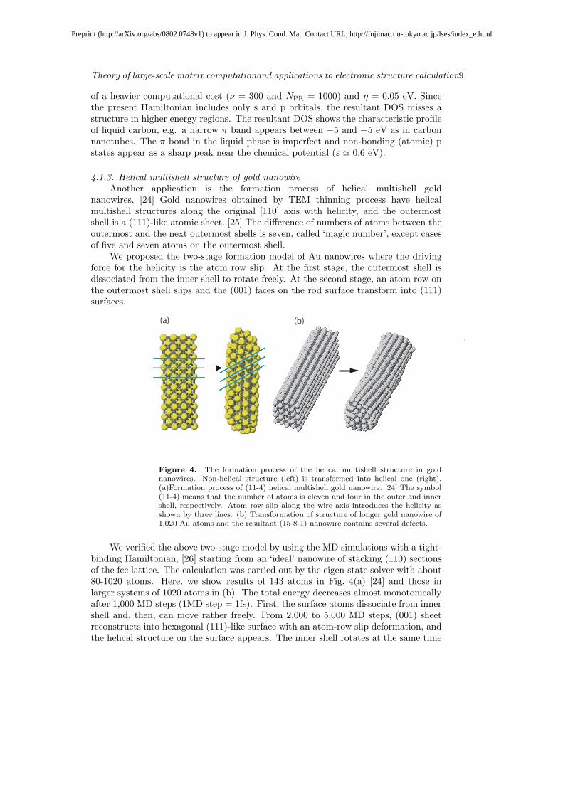
4.1.3. Helical multishell structure of gold nanowireAnother application is the formation process of helical multishell gold

nanowires. [24] Gold nanowires obtained by TEM thinning process have helicalmultishell structures along the original [110] axis with helicity, and the outermostshell is a (111)-like atomic sheet. [25] The difference of numbers of atoms between theoutermost and the next outermost shells is seven, called ‘magic number’, except casesof five and seven atoms on the outermost shell.

We proposed the two-stage formation model of Au nanowires where the drivingforce for the helicity is the atom row slip. At the first stage, the outermost shell isdissociated from the inner shell to rotate freely. At the second stage, an atom row onthe outermost shell slips and the (001) faces on the rod surface transform into (111)surfaces.

(a) (b)

Figure 4. The formation process of the helical multishell structure in goldnanowires. Non-helical structure (left) is transformed into helical one (right).(a)Formation process of (11-4) helical multishell gold nanowire. [24] The symbol(11-4) means that the number of atoms is eleven and four in the outer and innershell, respectively. Atom row slip along the wire axis introduces the helicity asshown by three lines. (b) Transformation of structure of longer gold nanowire of1,020 Au atoms and the resultant (15-8-1) nanowire contains several defects.

We verified the above two-stage model by using the MD simulations with a tight-binding Hamiltonian, [26] starting from an ‘ideal’ nanowire of stacking (110) sectionsof the fcc lattice. The calculation was carried out by the eigen-state solver with about80-1020 atoms. Here, we show results of 143 atoms in Fig. 4(a) [24] and those inlarger systems of 1020 atoms in (b). The total energy decreases almost monotonicallyafter 1,000 MD steps (1MD step = 1fs). First, the surface atoms dissociate from innershell and, then, can move rather freely. From 2,000 to 5,000 MD steps, (001) sheetreconstructs into hexagonal (111)-like surface with an atom-row slip deformation, andthe helical structure on the surface appears. The inner shell rotates at the same time



of the atom-row slip. Analysis of electronic structure shows that the mechanism inboth stages is governed by the d-band electrons extending over the (111)-like surface,where the center of gravity of the d-band locates in the lower energy side. The helicalnanowires appear only among metals with a wider d-band, e.g. in Au and Pt butnot in Ag and Cu. Helicity is introduced by the surface reconstruction or the atom-row slip on the (001) sheet, because the triangular (111)-like sheet is more preferablefor d-orbitals extending over the surface. The d-band width in platinum and gold iscommonly wider than that in lighter elements, Ag and Cu, and the calculated resultexplains why platinum nanowire can be also formed with helicity.

4.2. Application to many-electron systems : Excitation spectrum of multi-orbitalextended Hubbard Hamiltonian on two-dimensional square lattice

The transition metal oxides have been paid a great attention due to their variousphysical properties which are drastically changed and controllable by external fieldsor doping. Here we show an application of the shifted COCG method to theextended Hubbard model with doubly degenerated orbital and the inter-site Coulombinteraction on a two-dimensional square lattice. [17] This is a model of La 3

2Sr 1

2NiO4

and we used a finite unit of N = 8 sites and the total number of electrons Ne = 32N =

12.

0.4

0.2

0

0.2

0.4

0 5 10 15 20

-1/π

Im

GR

(ω)(

1/eV

)

0.4

0.2

0

0.2

0.4

0 5 10 15 20

-1/π

Im

GR

(ω)(

1/eV

)

ω(eV)

0.4

0.2

0

0.2

0.4

0 5 10 15 20

-1/π

Im

GR

(ω)(

1/eV

)

Highest ionization level

V=0.5eV

V=0.2eV

V=0eV

Ionization level

Ionization level

Ionization level

Affinity level

Affinity level

Affinity level

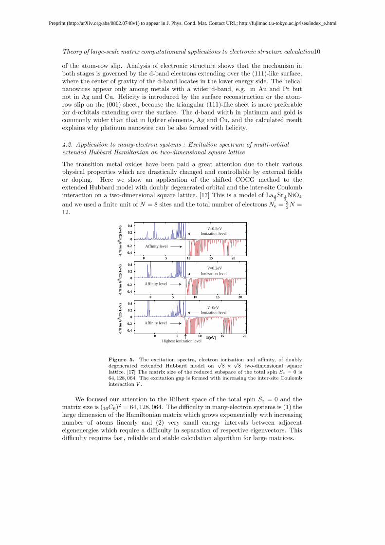
Figure 5. The excitation spectra, electron ionization and affinity, of doublydegenerated extended Hubbard model on

√8 ×

√8 two-dimensional square

lattice. [17] The matrix size of the reduced subspace of the total spin Sz = 0 is64, 128, 064. The excitation gap is formed with increasing the inter-site Coulombinteraction V .

We focused our attention to the Hilbert space of the total spin Sz = 0 and thematrix size is (16C6)2 = 64, 128, 064. The difficulty in many-electron systems is (1) thelarge dimension of the Hamiltonian matrix which grows exponentially with increasingnumber of atoms linearly and (2) very small energy intervals between adjacenteigenenergies which require a difficulty in separation of respective eigenvectors. Thisdifficulty requires fast, reliable and stable calculation algorithm for large matrices.



Figure 5 shows the excitation spectra of electron ionization and affinity levels andthe energy gap between these two corresponds to the excitation gap. Normally, theHubbard model of non-degenerate orbital, in case of the integer occupation, gives theinsulating gap due to the on-site Coulomb interaction and, on the contrary, in caseof non-integer occupation, the system is metal. Here, in the doubly degenerate case,the charge stripe order with an insulator gap is formed due to the inter-site Coulombinteraction V and, on top of that, the spin stripe is formed with anisotropy of electronhoppings. [17]

Crucial point is that we should keep very high accuracy of the computation forjudging the ‘gap’, compared with the ‘level interval’ in finite systems and that theiteration convergence should be controlled during the iterative calculation. Therefore,the capability of convergence (accuracy) monitoring and robustness are seriouslyimportant and the shifted COCG method can solve this difficulty.

5. Conclusions

We have reviewed our recently developed methods for large-scale electronic structurecalculation applied to both one-electron theory and many-electron theory. For large-scale systems of about 10’s nm scale, one can use several solver methods simultaneouslyas a multi-solver method. We also explained differences between two theories fromthe viewpoint of large-scale matrix computation. Then we presented examples ofthe applications of nano-scale systems, the formation and propagation of fracturein large silicon crystals, the MD simulation in liquid carbon, and the formationof helical multishell structure of gold nanowires and an example of many-electronproblems, the orbital degenerated extended Hubbard model. In these applications,we stressed the importance of the hybrid scheme of multiple solver methods and thenovel computational algorithm.

Acknowledgments

Numerical calculation was partly carried out using the supercomputer facilities of theInstitute for Solid State Physics, University of Tokyo.

References

[1] Comp. Sci. Eng., the January/February 2000 issue.[2] SIAM News, Vol. 33, No. 4.[3] W. Kohn, Phys. Rev. Lett. 76, 3168 (1996).[4] T. Hoshi and T. Fujiwara, J. Phys. Soc. Jpn. 69, 3773 (2000).[5] T. Hoshi and T. Fujiwara, J. Phys. Soc. Jpn. 72, 2429 (2003).[6] T. Hoshi, Y. Iguchi and T. Fujiwara, Phys. Rev. B72, 075323 (2005).[7] R. Takayama, T. Hoshi and T. Fujiwara, J. Phys. Soc. Jpn. 73, 1519 (2004).[8] R. Takayama, T. Hoshi, T. Sogabe, S-L. Zhang and T. Fujiwara, Phys. Rev. B73, 165108 (2006).[9] M. Geshi, T. Hoshi and T. Fujiwara, J. Phys. Soc. Jpn., 72, 2880 (2004).[10] T. Hoshi, and T. Fujiwara, J. Phys: Condens. Matter. 18, 10787 (2006).[11] F. Mauri, G. Galli and R. Car, Phys. Rev. B47, 9973 (1993).[12] N. Marzari and D. Vanderbilt, Phys. Rev. B56, 12847 (1997).[13] I. Kwon, R. Biswas, C. Z. Wang, K. M. Ho and C. M. Soukoulis, Phys. Rev. B 49, 7242 (1994).[14] C. H. Xu, C. Z. Wang, C. T. Chan and K. M. Ho, J. Phys. Condens. Matter 4, 6047 (1992).[15] O. K. Andersen and O. Jepsen, Phys. Rev. Lett. 53, 2571 (1984).[16] http://elses.jp[17] S. Yamamoto, T. Fujiwara and Y. Hatsugai, Phys. Rev. B76, 165114 (2007).



[18] S. Yamamoto, T. Sogabe, T. Hoshi, S.-L. Zhang, and T. Fujiwara, in preparation.[19] C. Lanczos, J. Res. Natl. Bur. Stand. 45, 225 (1950); ibid. 49, 33 (1952).[20] M. R. Hestenes and E. Stiefel, J. Res. Natl. Bur. Stand. 49, 409 (1952).[21] A. Frommer, Computing 70, 87 (2003).[22] T. Sogabe, T. Hoshi, S.-L. Zhang, and T. Fujiwara, Frontiers of Computational Science, pp. 189-

195, Ed. Y. Kaneda, H. Kawamura and M. Sasai, Springer Verlag, Berlin Heidelberg (2007).[23] K. C. Pandey, Phys. Rev. Lett. 47, 1913 (1981).[24] Y. Iguchi, T. Hoshi and T. Fujiwara, Phys. Rev. Lett. 99, 125507 (2007).[25] Y. Kondo and K. Takayanagi, Science 289, 606 (2000).[26] F. Kirchhoff, M. J. Mehl, N. I. Papanicolaus, D. A. Papaconstantpoulos and F. S. Khan, Phys.

Rev. B63, 195101 (2001).


Documents

Theory of large-scale matrix computation and applications ...coral.t.u-tokyo.ac.jp/hoshi/doc/2008_Fujiwara-arXiv_0802_0748.pdf · and applications to electronic structure calculation