a __ __ !!B 15 June 1997

OPTICS COMMUNICATIONS

ELSEVIER Optics Communications 139 (1997) I-6

Theory for the propagation of short electromagnetic pulses

Nicholas George I , Stojan Radic

CenrerfiJr Electronic Imaging S_vsremu. The lnstitufe of Optics. Utzicvrsig of Rochester. Rochester, NY 14627. USA

Received 18 November 1996; accepted 8 January 1997

Abstract

A theory is presented for the free-space propagation of short pulses of any duration, including sub-cycle or unipolar

pulses. From Maxwell’s equations, we provide an exact solution of the vector potential and the scalar potential which result for an electric dipole created stepwise at t = 0 with a corresponding Dirac-delta in source current density. This idealized unipulse provides valuable insight as to the separation of 1 /r propagating terms from those of higher order arising from the

scalar potential. Secondly, an exact solution is presented for the radiation field in temporal form which arises from an assertion of an input aperture distribution. Since the temporal assertion may lead to propagation terms of l/r dependence and others of higher order, we illustrate how to make an informed choice. A finite-difference-time-domain computer study of

four selected sub-cycle pulses is used to illustrate the method and to verify our prediction that free-space propagation is a linear filter of temporal frequency varying as [iZrrv/(rc)] expt - i?rrvr/c) with a null at zero frequency.

1. Introduction

With the advent of ultra-wideband pulse radars, consid- erable attention has been directed to various aspects of the generation, propagation. and reception of this electromag-

netic radiation. Since the free-space propagation of an

ultra-wideband (UWB) pulse is within the domain of Maxwell’s equations, it is important to present a rigorous

framework for the solution of the many important prob- lems arising. This is handy as a benchmark for comparison of results using the important computer method finite-dif-

ference time-domain (FDTD) and the equally important methods of Fourier optics.

In this material we present two different idealized problems dealing with the propagation of ultrashort unipo-

lar pulses. First, as an idealized but realizable source, we

consider the creation of an electric dipole, using the Heavi- side step function U(r). by a unipolar Dirac-delta function

impulse of current density J located at the origin. This source distribution is helpful to develop understanding since it provides insight into the propagation of the I/r fields and in contrast to the static field as well. Also,

I E-mail: ngeorge@troi.cc.rochester.edu.

interestingly, the static field is readily separated since the

electric dipole remains “on” as t --) cc. Next, we describe the calculation for radiation from an

aperture using an “assumed” distribution of electric field. This type of source problem is often termed a secondary

source. We show that some care needs to be exercised in

this assertion of a specific temporal behavior. The field can have propagating and higher order components. In any

event we are able to write a theoretical form for the solution of the radiation from an open aperture. This will be recognized as a fruitful avenue for further research. It is

clear from this example that one can rewrite the vector diffraction integral equivalents of Maxwell’s equations in a

time-dependent fashion. For brevity in our presentation,

we started from the well-known Rayleigh-Sommerfeld-

Smythe form. However, for theoretical purposes it would be more satisfying to start with a time-dependent form of

Maxwell’s equations. Appealing theoretical avenues are

the single and double-sided Laplace transforms [ 1,2]. Re- lated early literature on an electric dipole stepped on at t = 0 is contained in Sommerfeld’s lectures [3] and in an article by B. van der Pol 141. Equations for pulsed antennas and for the transient response of an infinitesimal dipole of

moment p(t) are given in a monograph by C.H. Papas [5].

Two other references have been found in which a Dirac-

0030-4018/97/$17.00 Copyright 0 1997 Elsevier Science B.V. All rights reserved p/l SOO30-40 I8(97)00038-2

2 N. George, S. Radic/ Optics Communications 139 f 1997) 1-6

delta impulse is used to turn on the electric dipole [6,7]. In these latter two, the current is no longer unipolar. They use a Coulomb-gauge, and so the relevance to the UWB propagation is not as direct.

2. Propagation from an impulse in current

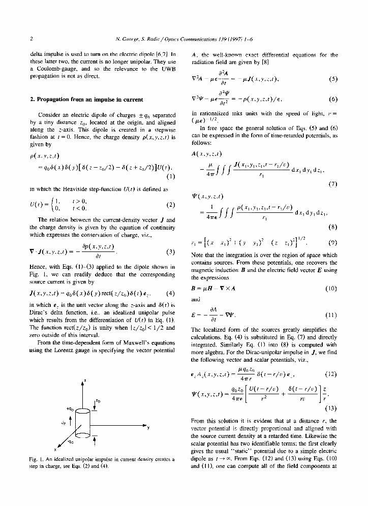
Consider an electric dipole of charges fq, separated by a tiny distance za, located at the origin, and aligned along the Z- axis. This dipole is created in a stepwise fashion at r = 0. Hence, the charge density p(x, y,z,r) is given by

in rationalized mks units with the speed of light, L’ = ( /Je)- “2.

In free space the general solution of Eqs. (5) and (6) can be expressed in the form of time-retarded potentials, as follows:

P( x,Y,Z,r) A( x,y,~,r)

CL ///

J(X1.Y ,,z,,r-r,/L’) =-

4%- rl dx, dy, dz,,

(7)

= qoq x)S( Y>[ q z - zo/q - 6( z + z,/2)]U(r), (1)

in which the Heaviside step-function u(t) is defined as

U(t)= ;, L t>o, t < 0.

The relation between the current-density vector J and

the charge density is given by the equation of continuity which expresses the conservation of charge, viz.,

dp( X,Y,ZJ) V.J(x,y,z,t)= - dr

Hence, with Eqs. (l)-(3) applied to the dipole shown in

Fig. 1, we can readily deduce that the corresponding source current is given by

J( x-,~,z,t) = qo6( x)S( y)rect( z/+)8(r) e,, (4)

in which eL is the unit vector along the z-axis and s(t) is Dirac’s delta function, i.e., an idealized unipolar pulse

which results from the differentiation of U(f) in Eq. (1). The function rect( z/z,) is unity when 1 Z/Q/ < l/2 and

zero outside of this interval.

From the time-dependent form of Maxwell’s equations using the Lorentz gauge in specifying the vector potential

z

-+

=o

+qo -

JZ t,

-

-t

Fig. I. An idealized unipolar impulse in current density creates a

step in charge, see Eqs. (2) and (4).

A, the well-known exact differential equations for the radiation field are given by [8]

1

V’A - pe? = -pJ(x,Y,z,r), (5)

2

v*- PC:: = -p(x,.v,i,t)/E, (6)

T(x,,,z,t)

1

Jil

P(x,,Y,*z,,r-r,/u) =- 4%-e

dx, dy, di,, rI

(8)

‘,=[(X-xx,)~+(Y-y,)~+(z-Z,)~]“2. (9)

Note that the integration is over the region of space which

contains sources. From these potentials, one recovers the magnetic induction B and the electric field vector E using

the expressions

B=p,H=VXA (‘0)

and

E= -z-w. (11)

The localized form of the sources greatly simplifies the

calculations. Eq. (4) is substituted in Eq. (7) and directly integrated. Similarly Eq. (1) into (8) is computed with

more algebra. For the Dirac-unipolar impulse in J, we find

the following vector and scalar potentials, viz.,

eLA;(x,y,z,~) = F 6(t-r/u)e,, (12)

cl020 U(t - r/u) ~(x,y,z,t)=~

[ r2 +

s(t-r/u) 2

ru l- r’

(13)

From this solution it is evident that at a distance r, the vector potential is directly proportional and aligned with

the source current density at a retarded time. Likewise the scalar potential has two identifiable terms; the first clearly

gives the usual “static” potential due to a simple electric dipole as t + m. From Eqs. (12) and (13) using Eqs. (10) and (1 l), one can compute all of the field components at

N. George. S. Rndic / Optics Communications 139 (19971 l-6

an arbitrary position f x,v,z). In the interest of brevity, we will calculate only the spherical component of the electric field, &, where H is the spherical polar coordinate of an (r, 0, I#J) system. This transverse component of electric field serves as a good indicator of the entire propagation field. For the Dirac-impulse source current, the transverse component of the electric field EH is given by

+ q,,:, U(t - r/r)

[ +

S(r - r/lx)

he ri rZ L: I

sin@. (14)

Note that the derivative of the delta function, S’(t), can be represented by the following limit form:

S’(r) = lim Z crt

cu>o. u-0 7r ($ + o2)? ’ (‘5)

Clearly by Eq. (15). the derivative of the Dirac-delta is seen to have a large positive lobe at negative argument followed by a large negative lobe for positive argument.

Now in Eq. (14) only the term falling off with distance as l/r represents propagation (in the radar sense). At large distances the scalar potential (last 2 members) does not contribute a meaningful signal. Most interesting in Eq.

(14) is the absence of a unipolar-component (dc) in the propagating term with the 1 /r dependence. This is evident

from the bipolar nature of the S’(t) in Eq. (1.5). Hence

from Eqs. (41, (I 2) and (14), we have established that the radiation field due to a Dirac-delta-unipulse in current density leads to a “following” unipulse in the vector

potential at retarded time but to a bipolar impulse in the electric field.

3. Radiation from apertures (time-dependent)

For an infinitesimally thin perfectly conducting sheet in the plane at z = 0 with an open aperture letting radiation

from sources (; < 0) propagate into the right-half-space, one can calculate the radiation for z > 0 in terms of the tangential electric field in the aperture. The coordinate

axes here should not be confused with the choice used in the earlier sections. Here, we are considering the z-axis as

the axis of propagation, as is customary in the Rayleigh- Sommerfeld-Smythe formulation. The electric field E(r) in the right half-space, i.e., z 2 0, is then uniquely speci- fied by the tangential component of the exact electric field

in the aperture 19, IO]:

(‘6)

where

r,~lr-r’/=\/(x-xx’)‘+(y-y’)Z+z”. (17)

exp( - i kr, l/r, is the free-space Green’s function, n is a unit normal pointing in the fz direction, and &r’) is the exact electric field in the aperture. The integration extends only over the aperture because the screen is a perfect conductor.

In the signal representation of the electric vector f?(r’), we have used the “tilde” to specify that we are dealing with the temporal Fourier transform of the time varying electric field. Moreover, we emphasize that the time-vary ing function has been written in an analytic signal form.

Hence, in definition of the signal notation, one can write

i(r;v) = jX E,(x,~,z;r)e-‘2a”‘dr, -*

(18)

and the Fourier inversion:

E,(x,y,z;t) = jX E(r;Y)e+“““dV. -r

(‘9)

The subscript ‘a’ denotes an analytic signal form. Note as well that the harmonic time dependent analysis using exp(iot) would yield a formula that is notationally as given by Eq. (16) with 27r~ = o.

It is useful to write out explicitly the expressions for all three components of the electric field transforms:

#Q x,y,z) = ; j j ~.~(X’,Y’,O) exp( - ikr,)

A TI

X(ik+-l-)(;i-)dr’d;‘,

k,(x,.v,z) = ; j jAE,(+‘,LO) exp( - i kr, )

r,

x(ik+-!-)(t)di.dr.,

E;(x,y,z> = & /jJ (Y) G’,V’~O)

+ (+) E,(x', y’,O)]

(20)

(21)

X exp( - ikr, )

rl (22)

Note too that k = 27rv/u and for an UWB pulse this variable changes dramatically. Hence, the output ,!?,( x, y, z 1

is governed by !o%,< x, v,O). For the UWB pulse calculation in some instances, we

would prefer to select a time-dependent incident field for our calculation. It is insightful to derive a time-dependent

aperture formula for the radiation into the right-half-space.

This is easily obtained simply by Fourier inversion using

N. George, S. Radic/ Oprics Communications 139 (IY!?7) 1-6

Fig. 2. Configuration for FDTD calculation with slit width )I’ = 5.55A and distance P = 14.44h.

Eq. (19). For purposes of illustration, it is adequate to invert Eqs. (16) and (21). Hence, radiation can be calcu- lated from the following aperture forms:

E,( x,.v,z;r)

R x E,( x’,y’,O;t - r-,/u) dx’ dy’,

YI

(23)

+ E,,( x’,y’,O;t - r,/u> 27rrF 1 dx’dy’,

(24)

it is instructive to compare Eqs. (23) and (24). As a typical

problem, one would like to assert a time-dependent form at the aperture and then calculate the fields propagating to an

arbitrary point (x, y,z), as in Fig. 2. From Eq. (23) we have the well-known operation of retarded time r + I - I-,/u. By the expansion of Eq. (24) one observes that the

scalar component of tangential electric field can be sepa- rated into a term containing a/&[ E?,] that propagates with l/r range dependence and a second term containing

[E?,] that propagates as l/r’. In summary for an arbitrary

aperture distribution E?.,(x, y,O;t), we see that the radia- tion field will have a bipolar form as evidenced by the

time derivative a[ E,.,]/& in Eq. (24).

4. Finite-difference time-domain calculation of near- field evolution for incident unipolar signal

Starting from Yee’s original idea [ 111, finite-difference

time-domain (FDTD) methods have played an important role in the establishment of a number of rigorous solutions of Maxwell’s equations. During the 1960s and 1970s

FDTD methods have been successfully used for complex EM scattering problems that include radar cross sections,

human tissue imaging, and high-speed circuit design [ 12- 141. In the 1980s and more recently, an increasingly important role has emerged for the FDTD approach in ultrafast optoelectronics and photonics [ 15 191. A number of important advances that include generalizations encom- passing dispersive and nonlinear materials [ 15,161 have allowed modeling of soliton propagation, ultrafast switch- ing, and dispersive periodic structures [ 18,191. Combined with current developments in ultrafast optics that lead to sub-cycle pulse generation and breakdown of any approxi- mation (slow-envelope, small perturbation strength) the generalization of FDTD methods will serve as a preferred, and often the only rigorous tool at our disposal. Dispersive or nonlinear properties of the medium are readily incorpo-

rated into the method as we previously described [ 191. The physical limitation to such a rigorous approach is three-fold: (a) computing resource (speed), (b) available memory storage, and (c) boundary condition implementation. Even

as we are writing these lines, an improvement in condition (a) is being made by a new generation of fast parallel

processing architectures. Condition (b) currently limits our calculation to 50 X 50 wavelength size in 2-D and 15 X 15 X 15 wavelength size in 3-D for a very fast (non-buffered)

computation. Finally, condition (c) has been a subject of substantial research in the last two decades [20-221, yield- ing some exceptional boundary algorithms. The role of

FDTD boundary condition is to limit computation size without introducing any artificial (numerical) diffraction at the boundary of the modeling site. We are currently using

Engquist-Majda [22] condition which introduces an error

of - 10-j.

In this research on the diffraction and propagation of subwavelength pulses, Eqs. (23) and (24) permit one to

select ad-hoc pulse envelopes to use as secondary sources. However, when we use an assumed value for the tangential

field, it often will contain terms that propagate as (l/r) and higher order terms dropping off as l/r2. We believe that FDTD methods are ideally suited to test this notion, since they provide an exact numerical solution. Terms

arising, in effect, from a scalar potential will drop ex- tremely fast. Typically by Eq. (201, one can estimate that

in the near zone the ratio of the propagation term to the near-field term will be increased on the order of h. To test the validity of this notion, we need to examine the evolu-

tion of an assumed subwavelength pulse in the near field.

We expect the form to change rapidly at first, thereby placing in evidence a bipolar remainder term which is

essentially entirely a propagation term falling off more

gradually as (l/r). For the FDTD calculation, consider an aperture in a

conducting plane at z = 0 with the radiation incident from

the left, shown in Fig. 2. For an incident plane wave (A = 0.9 mm) diffracted by a large aperture (5.55h wide), we calculate the resulting field after propagation to a point P, 14.44A away. At P, this field history is stored and used to calculate spectra, as shown in Figs. 3a-3d. As illus-

N. George, S. Radic / Optics Communications 139 (1997) 1-6 5

trated in our earlier theory, the temporal dependence con- sists of a propagating (“dynamic”) portion and a “static” one. Our assertion is that FDTD calculation of the field at R, > 14A is an excellent demonstration of “static” field filtering. Figs. 2a-2c show inputs (dashed) which are synthesized with a strong unipolar component. The solid curve shows considerable modification due to the filtering of the near-field components. Alternatively, Fig. 2d shows a less drastic modification due to the initial choice of a

bipolar form; i.e., one complete cycle of a sine wave.

5. Impulse response and transfer function for free-space

From Eqs. (20) and (2 1) in Fourier optics, it is custom- ary to note the perfect convolution of the input, I?,(x, y,O; v), with the normal derivative of Sommerfeld’s choice for the Green’s function. This function is termed the impulse response h(x - .r’,v - $;v) and is given in

Ref. [23] by

h( x,v;v) = exp( -ikr) 2 i2rv

*nr ,(,+$ P)

in which r = (.I-’ + x’ + ;‘)“‘. However, if we consider

the temporal dependence of the input E,,(x, v.O;r) and the

440 46.0 46.0 50.0 52.0

& 440 46.0 48.0 50.0 520

44.0 46.0 46.0 50.0 52.0

Ti

44.0 46.0 48.0 50.0 52.0

a

b

C

d

temporal Fourier transform, e.g., in Eq. (18), then it is appropriate to consider that h (x, y; v> is a “transfer-func- tion” insofar as its temporal origin, i.e., in the v variable.

This interpretation lends clarity to the spectral curves in Fig. 3, since we see that the l/r term has a transfer function proportional to the term i2nu exp( - i2nv r/c). Insofar as the temporal frequency dependence, this zero in the transfer function explains the intuitive filtering-out of the “static or dc component” hypothesized in the initial

aperture distribution. Again the same observation can be drawn for the

idealized unipolar pulse in Eq. (4). The radiation term given by the retarded vector potential [A] in Eq. (7) has

the &function form. Hence in computing the correspond-

ing electric field by taking a time derivative leads to the s’(t) in Eqs. (14) and (15). Finally, considering this S’(r) as an impulse response, we take the temporal Fourier transform to find the transfer function. Since ,7 6’(r) =

i2av we find a consistent explanation.

Acknowledgements

The authors are pleased to acknowledge the helpful comments by B.D. Guenther and the support of the Army Research Office and the National Science Foundation.

Ki -1 .o -0.5 0.0 0.5 1.0

I 1 I I 1

1 ~~,,~~ -1 .o -0.5 a.0 0.5 1.0

/ .

-1 .o -0.5 0.0 0.5 1.0

11 -1 .o -0.5 0.0 0.5 1.0

Fig. 3. Finite-difference time-domain solutions for the pulse shapes (dashed) in the aperture after propagation (solid) to P at ; = 14.44h,

shown in Fig. 2. Corresponding spectra are also shown (dashed in aperture and solid at P).

6 N. George, S. Radic/Optics Communications 139 11997) 1-6

References

[I] H.S. Carslaw and J.C. Jaeger, Operational Methods in Ap-

plied Mathematics, 2nd Ed. (Oxford University Press, Lon- don, 1947).

[2] B. van der Pol and H. Bremmer, Operational Calculus Based

on the Two-Sided Laplace Transform, 2nd Ed. (Cambridge

University Press, London, 1955).

[3] A. Sommerfeld, Vorlesungen ilber theoretische Physik, Band

III, Electrodynamik (Wiesbaden, 1948) p. 150.

[4] B. van der Pal, IRE Trans. Antennas Propag. AP-4 (1956)

288.

[5] C.H. Papas, Yerevan Lectrures on Electromagnetic Theory

(California Institute of Technology Press, Pasadena, 1972)

Ch. 9.

[6] O.L. Brill and B. Goodman, Amer. J. Physics 35 (1967) 832.

[7] J.D. Jackson. Classical Electrodynamics, 2nd Ed. (Wiley,

New York, 1975) prob. 6.19, p. 267. [S] W.R. Smythe, Static and Dynamic Electricity, 3rd Ed., re-

vised (Summa-Hemisphere, New York, 1989) Ch. XII.

[9] W.R. Smythe, Phys. Rev. 72 (1947) 1066.

[lo] R.E. English and N. George, Appl. Optics 26 (1987) 2362.

[I 11 K.S. Yee, IEEE Trans. Antennas Propag. AP-14 (1966) 302.

[12] K. Umashaukar and A. Taflove, IEEE Trans. Electromag.

Compat. EMC-24 (1982) 397.

[13] KS. Kunz and K.M. Lee, IEEE Trans. Electromag. Compat.

EMC-20 (1978) 328.

[14] A. Taflove, Computational Electrodynamics: The FDTD

Method (Artech House, 1995).

[15] R.M. Joseph, S.G. Hagness and A. Taflove, Optics Lett. 18

(1991) 1412.

[16] P.M. Goorjian, A. Taflove, R.M. Joseph and S. Hagness,

IEEE J. Quantum Electron. 28 (1992) 2416.

[ 171 A. Taflove, Wave Motion (1988) p. 547.

[18] R.M. Joseph and P.M. Goorjian. Optics Lett. 48 (1993) 491.

[19] S. Radic and N. George, Optics Lett. 19 (1994) 1064.

[20] J.G. Blaschak, J. Comput. Phys. 77 (1988) 109.

[21] J.P. Berenger, J. Comput. Phys. 114 (1994) 185.

1221 B. Engquist and A. Majda, Math. Comput. 31 (1977) 629.

[23] N. George, Optics Comm. 133 (1997) 22.