Theories of Causal Ordering -

ARTIFICIAL. INTELLIGENCE 33

Theories of Causal Ordering

Johan de Kleer and John SeelyBrownIntelligent SystemsLaboratory,XEROX Palo AIto ResearchCenter. Palo Alto, CA 94304, US. A.

Recommendedby Daniel G. Bobrow

ABSTRACT

ibis paperis a responseto Iwasakiand Sitnon 141 which criticizesde KleerandBrown I~I.We arguethat loans of tilt ir ( run ions partuularl~ nun mint, t ausaltts unodtlint, and stab,lzti, 0z lynaut trounthe differenceof concernsbetweenengineeringand economics.Our notion of causalityarisesfromconsiderzngthe interconnecuionsof components not equations.Whenno fet’dhack is present. theorderingproducedby our qualitativephysicsis similar to theirs. However,whenfeedbackis present,our qualitative physicsdeterminesa causalordering aroundfeedbackloops as well.

Causalordering is a generaltechniquenot out/v applicableto qualitative reasoning. Thereforewealso explorethe relations/zip betweencausalordering andpropagationof constraintsupon which theunelhod5 of qualutatiic ph vsics are based.

1. Introduction

Many of the differencesbetweenthe paperby Iwasaki and Simon [‘41’ andthatby de Kleer andBrown [81 originate from a difference in point of view on therelationshipbetweenthe structureof a systemandthe equationswhich describeits behavior. We believe that this difference stems, in large part. from adifferencein explicitnessof the mechanismsand structuralcomponentsunderly~ing economicsystemsversusengineeredartifacts.We hope that the mergingofthe theoreticaltechniquesandarsenalof tools of economicsandengineeringwilllead to a better understandingof the relationship between structure andbehavior,adeepertheoryof qualitativereasoning,and morepowerful tools for

qualitative analysis.A standardeconomicapproachto analyzing a situation starts with a set of

equilibrium conditionsand a set of differential equationswhich describethedynamic processwhich underliesthe equilibrium equations.To determinetheresponseof the systemto a disturbanceone first checkswhether the dynamicprocess can approach a new equilibrium, and if so, uses the method of

All references in this paperto Iwasaki and Simon refer to 1141.Artificial Intelligence29 (1986) 33—A I

0004-3702/86/$35()© 1986, Elsevier SciencePublishers WV. (North-Holland)

34 J. DE KLEER AND JS. BROWN

comparativestatics to calculatethe new stableequilibrium. Causal ordering17, 181 placesan orderingon the variables.Oversimplifying, when a variable

canbe solvedby simplesubstitutionsit is causallydependenton the antecedents,howeverwhen a variablecannothe solvedthroughdirect substitution(i.e., theequationsdescribea feedbackloop), no causalorderingis indicatedamongthevariablesof the loop.

A standard engineering approachto analyzing a device starts with itscomponentsand connections. Componentsand their associatedconnectionsobeycertainlaws. To determinethe responseof the systemoneformulatesa setof equationsspecifiedby theselaws andsolves this set to determinea response.An electricalengineer,for example,presumesa systemis alwaysat equilibrium(e.g., Kirchhoff’s current and voltage laws are equilibrium conditions fornetworksfill). By referring to the componentsand their interconnections,heproducesa completecausal pathway from input (specifically identifying thecausalorderingscorrespondingto feedbackaction) to output.

From these thumbnail sketcheswe identify two central differences in ap-proachbetweenthe economist and the engineer.

—Causality.Providedonly with the structuralequationswhich haveno directrelationshipto the physical components.the strongestnotion of causality theeconomistcan imposeis dictatedby the form of the equations.The engineer’snotion of causalityon the other handderivesfrom the relationshipbetweentheequationsand their underlyingcomponentswhichcomprisethe modeledsystem.

— Feedback.The consequencesof thesediffering notionsof causalityaremostacutewhenthe equationsare inherentlysimultaneous(cannotbesolvedthroughdirect substitutions).As one ordering amongthe variablesof such a minimalcompletesubsetis indistinguishablefrom any other, tio ordering is preferredover any other for the economist. However, to the engineer,the inherentsimultaneityarisesout of a feedbackpath.andonedireclion arounda feedbackpath is always more natural than the others.Qualitative physics identifies thispreferredordering.

1.1. Range of applicability

Our qualitativephysicsis basedon a qualitativeintegralanddifferential calculus

16, 8, 22,231. It allows us to analyzesystemswhosebehavioris describedby,possibly nonlinear, ordinarydifferential equations.A wide variety of physicalsystems(e.g.. electrical, thermal, fluid, mechanical)can be characterizedbyordinary differential equations. Such systemsare typically called lumped-parametersystems,andare the subjectof an entirediscipline—systemdynamics[161. Someimportant typesof physicalsituationsfall outsideof our qualitativephysics.Distributedsystems,suchasairplanewings, the weather.flow in a river,

~1is the better referenceon causalordcring

THEORIES OF CAUSAL ORDERING 35

are characterizedby partial differential equationswith respect to spatialvariables.Although most movementcanbe parameterizedandthus describedby ordinarydifferential equations,mechanicalsystemswhich actuallyrearrangetheir parts and interconnectionsare difficult to model. Such reasoningaboutconnection,disconnection,andshapeof physicalcomponentsis, as yet, outsideof the scopeof our qualitativephysics.However,Forbus’ [121 qualitativeprocesstheory can be used to reasonabout devicesthat changetheir topology whileoperating.

Qualitative reasoningabout physical systemsis a rapidly expandingareaofresearch.However, in this reply we focus, as Iwasaki and Simon do, on thepaperby de Kleer and Brown [ 8].

1.2. Qualitative reasoning

We use Fig. 1 to contrastour approachto qualitative reasoningto that ofconventional physics and that of Iwasaki and Simon. The approachestakedifferent trajectories (Fig. 1) from the physical situation to the qualitativedescription of behavior. In each approach,certain steps are formalized andautomatized (e.g., equation solving), while others are not and must beperformedby a person.

In the qualitative physicsapproach,oneis providedwith a descriptionof thephysical situation in terms of componentsand their interconnections.We callthis the device topologyof the situation(e.g., in electronicsthe device topologycorrespondsto the schematic). Each component is modeled by a distinctequationandthusthe behaviorof the overall systemis characterizedby a setofqualitative differential equations. One analyzes this system of qualitativedifferential equations,exploiting its relationship to the structure,to obtain aqualitativedescriptionof the behaviorof thesystemand a causalaccountof howthat behaviorarises.Diagrammatically,qualitative physics follows edges(4)—(5) in Fig. 1. Both of thesestepsare automatized.

In the more general, conventional approach, oneis providedwith an informaldescription of the physical situation. The first step is to construct a set of

2

1 Differential solve Analytic

~~__2-°~Equations es Solution

Physical Situation

e1

.-~-~ Qua itatuve solve Common-SenseDifferential ~tescriptionEquat i Otis

Fm. 1. Qualitative reasoning.

36 1 DE KLEER AND J.S. BROWN

differential equationswhich characterizethe behaviorof the system.Onesolvestheseequationsto find an analyticsolution. Finally, oneinterpretsthis solutionto obtain a qualitativedescriptionof how the systemfunctions.Diagrammatical-ly, conventionalphysicsfollows edges(1)—(2)—(3)in Fig. 1. The modeling(1)and interpretation(3) stepsare insufficiently formalized to he automated.

Likewise, following the approachof lwasaki andSimon one starts with aninformal descriptionof the physical situation.Onefirst identifies the fundamen-tal mechanismsoperative in the physical situation, modeling each with aquantitative structuralequation. Ignoring, for the moment, the dynamic pro-cess, one usesthe method of comparativestatics to obtain a limited analyticsolution andthe methodof causalorderingto obtain a causaldescriptionfor thatsolution. This analytic solution is then interpretedby substitutingqualitativevaluesof the exogeneousvariablesto computea qualitative descriptionof thebehavior. Diagrammatically,the method of Iwasaki and Simon follows edges(l)—(2)—(3). Although the solving step (2) and the interpretationstep (3) areformalized, the modelingstep (1) is not.

This comparisonhighlights five importantdifferencesbetweenour approachand that of Iwasaki and Simon.

First, their approachdoesnot formalize the modelingstep(edges(1) or (4)).We argue in the remainderof this paperthat by downplayingmodeling,they losethe ability to causallyorder variableswithin feedbackloops. Presumably,theydeemphasizemodelingbecauseof an economicsbackgroundwhereit is usuallymore difficult to identify underlying componentsand interconnections.Al-though one could easily augmenttheir approachwith a modelingstep, thiswould still not allow one to identify a causalorderingwithin feedbackloopsbecausesuch causal ordering can only be determinedby referring to thecomponents—theirmethod is solely equation-based.

Second, their approachrequires solving a set of conventional differentialequations(i.e., they follow edge (2), not edge(5)), while qualitative physicsanalyzesthe systemby propagatingqualitative disturbancesthroughthe struct-ure. By requiringan initial setof conventionalstructuralequations,Iwasaki andSimon requireconventionalalgebrato determinethe qualitative behavior. Ourapproachdeterminesthe qualitative behaviorusingqualitative reasoningalone(i.e., without requiringthe quantitativeequationsor algebra).

Third, qualitative physics andconventionalphysics producea descriptionofthe behaviorof the systemover time while the method of Iwasaki and Simononly determinesthe initial responseof a systemto a disturbance.Iwasaki andSimon explicitly admit they ignore this issue (what we call interstatebehavior).However, by doing so, they miss a crucial advantageof qualitative reasoning.Qualitative physics providesa generalprocedurefor solving a set of possiblynonlinearqualitative differential equationsusing the qualitative analogto thecalculusof Newton and Leibniz. The equationsare qualitatively integratedtodeterminethe behavior of the systemover time. The method of Iwasaki and

THEORIESOF CAUSALORDERING 37

Simon presumesthe world is linear. Evenif they extendedtheir methodto dealwith nonlinearsystemsthey would he forcedto solve a systemof conventionalnonlinear differential equationsto determinethe qualitative behavior whilequalitative physics, basedon a qualitative integral and differential calculus,obtainsqualitative behaviordirectly.

Fourth, both types of qualitative reasoningare inherently ambiguous.Thequalitative operationsdo not define a mathematicalfield. As a result, theequationset may sometimeshe “indeterminate.”Just becausea subsetof thevariables is indeterminate does not imply that all combinations of thesevariables’valuesare consistent.Usuallyonly a few combinations(i.e., solutions)are consistent with the equations (we call these the behavioral modes orinterpretationsof the system). When provided with such an indeterminatesystem,comparativestatics producesa single incompletesolution (mentioningonly the unambiguousvalues),while qualitativephysicsidentifies all the globallyconsistentbehavioralmodes.

Fifth, our qualitative analysisproducesmore ambiguousresults than theirs.Our method producesqualitative behaviorusing qualitative reasoningalone.However, Iwasaki andSimon’s method producesthe qualitative behaviorusingquantitativeequationsandconventionalalgebra.Our approachhasthe advan-tagethat it applieswhenthe quantitativeequationsare unknownor nonlinearaswell as being computationallyfar simpler. However, when the conventionalequationsare known and manipulatingalgebraicexpressionswere permitted,Iwasaki and Simon’s approachproduces less ambiguity. This by no meansindicatesthat our behavioralmodesare spurious.The centralpredictivegoal ofqualitativephysicsis that (a) the behaviorof every physicaldevicewhich obeysthe original qualitative differential equations is described by one of thebehavioralmodes,and (b) every behavioralmode is realizedby some physicaldevicewhich obeysthe qualitativedifferential equations.(However,see[15] forsomeproblems.)Determiningthe minimal conditionsfor achievingthesegoalsisa major challengeof qualitative physics.

2. Propagation of Constraints

The propagationmethodusedin qualitativephysicsderivesfrom propagationofconstraintsas describedin [9, 19—211. In this sectionwe focuson propagationofconstraintsmore abstractlyin order to establisha comparisonbetweenit andthe methodof causalordering[181. In developingthis comparisonwe, for themoment, set aside any concernswith qualitativeness.We also discusstheadvantagesof propagationof constraintsfor solving systemsof equationsoverconventionaltechniquesand further argue that it provides a betterbasis forqualitative physics.

The intuitions behindconstraintpropagationoriginate from observationsofhow experiencedengineerssolve circuit equations.The neophyte engineer

38 .1. DE KLEER ANDiS. BROWN

analyzesa networkby explicitly formulating all the simultaneousequationsandsolving these. This approachleadsto complicatedalgebra, fails to highlightsignificantfeedbackpaths,anddoesnot identify goodplacesto makeapproxim-ations.

The expert engineeranalyzesthe network differently, neverexplicitly for-mulatingall the simultaneousequations.Instead,hestartsfrom the input to thenetwork, inspectswhat componentsare connectedto it, andinfers what othervoltages and currents must be as a consequenceof the laws governing thebehaviorof thesecomponents.This processiterates.Only when this style ofreasoningoverthe componentsgetsstuck,doeshe introducea feedbackvariablewhich he then symbolically propagatesaroundthe loop. For example, if hecannotdeterminea voltage acrossa resistor,then he actsas if he knows thisvoltageby introducinga variablex (we call x aplunkedvariable)to representit,inferring that the currentthroughit mustbe Rix, etc. This propagatedexpress-ion becomesmore complicatedas it is pushedaroundthe feedbackloop, untilthe loop is closedandthe resultingequationsolvedto eliminatethe introducedvariable.Furthermore,if the original input is symbolicor any of the componentparametersare symbolic, then all circuit quantitieswill be expressionsin termsof thosequantitiesf91~

The experiencedengineer’sapproachis far simpler, requiresless algebra,requiresfewer variables,identifies the feedbackpaths,and is less proneto errorbecausethe symbolic expressionsare lesscomplicated.Oneimportantaddition-al reason it is less prone to error is that he propagatesfamiliar expressionsthroughthe circuit topology.The expressionsare in termsof familiar variables.The expressionsare familiar in form in that they refer to the importantconceptualentitiesin the functioning of the system.Tile transformationson theexpressionsare familiar as eachresultsfrom a specific componentlaw andis notsimply a symbolicmanipulation.At every point the expressionhassignificanceto the experiencedengineer,he is neverblindly solving equations.This ideaofexploiting the connectionbetweenthe structureof the device andits structuralequationsto facilitate determiningthe solution is central to propagationofconstraintsand to qualitative physicswhich is basedon it.

The propagationmethod used by Iwasaki and Simon derivesfrom [18]. Itis unfortunatethat the relationshipbetweencausalorderingandpropagationofconstraintswasnot noticedsooner.The causalorderingideasof [18] shouldhavebeen incorporated in propagationof constraintslong ago. Fortunately, it isrelatively easy to exploit causalordering within propagationof constraints.Propagationof constraintsis nondeterministic,discoveringmultiple orderingsincluding, but not restrictedto, Simon’scausalordering, It is possibleto restrictpropagationof constraintssuch that it only generatesSimon’s causalordering.

2.1. The algorithm

Propagationof constraintsoperateswith a setof constraintsE (componentand


connectionlaws) which constrain the values of variables V (associatedwithattachmentsof connectionsto components).In the procedure,the valuesof thevariables are representedby cells, which, initially empty, contain varioustemporary symbolic expressionsduring the process,and at the conclusioncontain the computedvalue for all the variables.The algorithm temporarilymarks certain variablesas plunked.The basic stepsare:

Step1. Propagation. If enoughof the cells linked to a particularconstraintarenonempty, then perform the necessarysymbolic algebra to determine theunknowncell in termsof the known ones.Go to Step1. (Forexample,giventheresistorconstrainte = iR, if R and i areknown, then e = iR is propagated,if Rand e are known, then i = dR is propagated,and if e and i are known, thenR = eli is propagated.)

Step2 Solving. If all the cells linked to a particularconstraintare nonempty,then substitute the values into the constraint equation,simplify, chooseanyplunked variable, solve for it, and assign its cell the result. (If thereare novariables to solve for, then, if desired,a consistencycheckcan be made.)Bysubstitution,eliminatethe plunkedvariablefrom every cell value(for efficiencythis operationis usually delayeduntil thecell value is accessed).Go to Step 1.

Step3. Plunking. If somecell is empty,mark thatvariable asplunked,createa new algebraic symbol representingthe cell, and assign the expressionconsistingof this symbol to the cell. Go to StepI. Notice that asa cell will havebecomenonempty,the subsequentpropagationstep1 will propagatea symbolicexpression.For example,supposethat x + y = 3 andx is plunked, thenStep 1placesthe expressionx — 3 in y’s cell. Thus Step I not only propagatessimplevalues,but also symbolicconstraints.This is the origin of the namepropagationof constraints.

In the generic version of propagationof constraints the choice of whichvariable to plunk is arbitrary. However, many variants of propagationofconstraintsspecify which variable to plunk. These specificationsare calledplunking heuristics.

Step4. Termination.If all cells arenonernpty,halt. If somevariablesremainplunked, then the original equationset is underdetermined.

Propagationof constraintscan he viewed as a generalizedform of Gaussianelimination. However, it is far more flexible than Gaussianelimination con-ceivedin termsof matricesandpivoting. Someof the advantagesof propagationof constraintsare that it— is ideally suited for performingsymbolic algebra (i.e., the parametersare

nonnumeric);— applieswhen the equationsare nonlinear;— applieswhen the operationsdo not define a mathematicalfield;— applieswhen the equationsare redundant;— is efficient evenwhenthe equationsare extremelysparse(as is almostalways

the case);

40 J. DE KLEER AND iS. BROWN

— keeps a close link betweena constraintand the componentit models,— allows the constraintset to be extendeddynamically.

‘I’he following redescriptionof the techniqueof propagationof constraintsisformulatedto facilitatecomparisonwith causalordering.Bearin mind howeverthat this reformulationhidesthe advantagesjust discussed.(Note that the stepsdo not correspondone-to-one.)

The algorithmstateswith equationsF, variablesV. andan initially emptylistS in which the solution is constructed.F is assumedto be consistent.

Step 1. Substitution. If E is empty, perform the substitutionswhich haveaccumulatedin S. If somevariablesremainplunked,then the original equationset is undertermined.In both casesthe algorithm terminates.

Step2. !‘ropagation. If anyequationmentionsexactlyonevariable,removeitfrom F, solvefor that variable,addthesolution to 5, substitutethe valueinto allthe remainingequationsof F, and go to Step1.

Step 3. Pivoting. If one (or none) of the variables of some equation isunplunked, remove it from F, reformulate the equation equating the oneunplunked(or any)variable in terms of the remaining,addthis equationto 5,eliminate the chosenvariable from all otherequationsof E and go to Step 1.

Step 4. Plunking. Mark any unplunkedvariablestill in F asplunked.Go toStep3.

The following is a worked-outexampleof usingconventionalpropagationofconstraintsto solvea set of equations.Wepresentthis exampleto help explicatethe methodof propagationof constraintsand to show its relationshipto causalordering. At this stage we are purely concerned with manipulating theequations,and are explicitly ignoring modelingand qualitativeness.As discus-sedlater, thevariantof propagationof constraintsusedin our qualitativephysicsis quite different than illustrated by this example.

Supposethe original equationset was:

x+y2, (Cl)

2x+y=3, (C2)

x+a+ b =3, (C3)

(C4)

w+t=2, (C5)

2w+t3. (C6)

Step 4 applies. Ally of x, y, w, or t are candidatesfor plunking. Supposewechoosex~~ indicatesthe variableis plunked). Step3 appliesto (CI) or (C2).Supposewe choose (Cl). As a consequencey = 2 — x~is added to S andsubstitutedinto (C2). The five remaining equationsare (C3)—(C6) and


2.v5-b (2— x5) = 3, (C7)

which simplifies to

x =

Step2 applies.(C7) is removed,x5= 1 is addedto S.andsubstitutedinto (C3).

The four remainingequationsare (C4)—(C6) andthe simplified (C3):

a+ h2. (C8)

Step 4 applies. Any of a, b, w or t are candidatesfor plunking. Supposewechoosea. Apply Step3 to (C8). As a consequenceb = 2 — a5 is addedto S andthe remainingequationsare (CS), (C6), and the simplified (C4):

(C9)

which simplifies to

w + 2a5= 3.

Step 3 applies, (C9) is removed,w = 3 — 2a~is addedto S leaving:

—2a5+t= —l , (ClO)

—4a5+t=—3. (Cli)

Step3 applies,t = 2a5— I is addedto S, and t is substitutedleaving:

a5= 1 . (C12)

At the conclusion

S = (a5= 1, t = 2a5—1, w = 3 —2a5,b =2— a5, x5

= 1, y =2 — x5)

and performing the substitutionwe obtain

x=y=a=b=w=t=l.

2.2. Causal ordering

The substitutionof variablesin propagationof constraintsordersthe variables.Supposewe ignore the substitutionsrequired to solve the plunked variable.

42 J. DE KLEER ANt) iS. BROWN

x* —m.y

m b e w ~- ix~ my w*____e~t

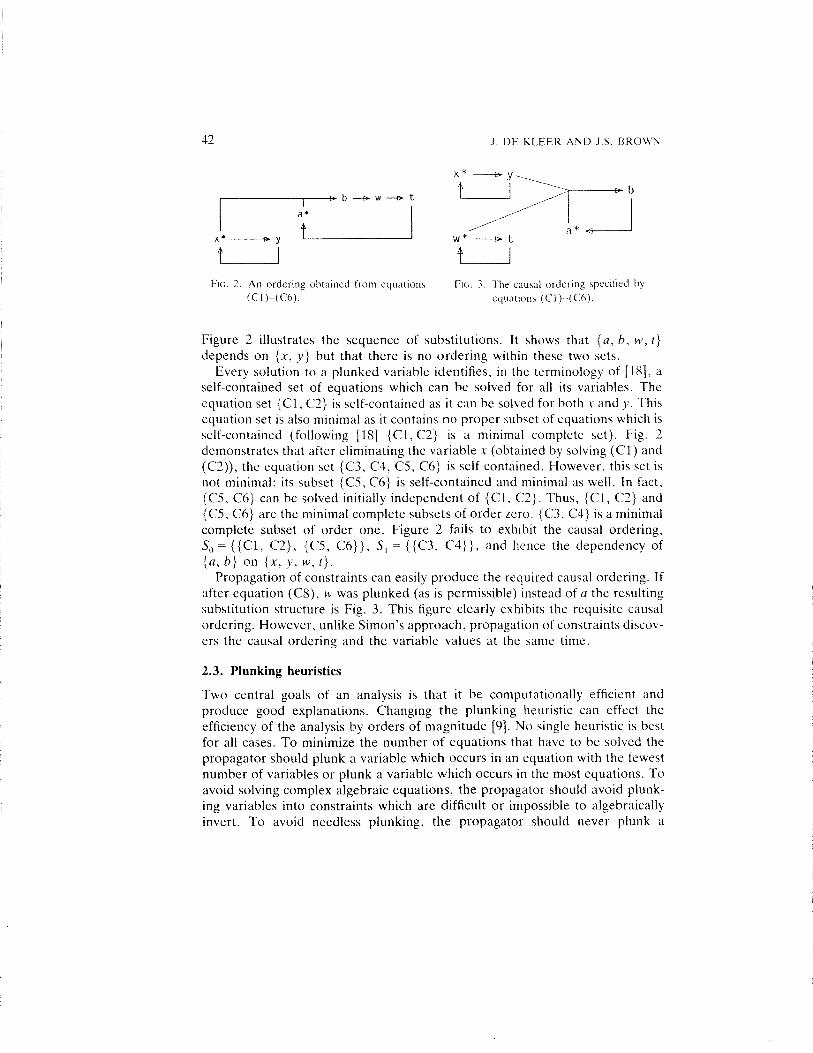
1 __Fie. 2. An orderingobtained from equations Lie .3. The causalordering specifiedby

(Cl )—(Cb). equations(Cl) —(Cfl).

Figure 2 illustrates the sequenceof substitutions. It shows that {a, b, w, t}

dependson {x, y} but that thereis no orderingwithin thesetwo sets.Everysolution to a plunkedvariable identifies, in the terminologyof [18], a

self-containedset of equationswhich can be solved for all its variables.Theequationset {Ci, C2} is self-containedas it canbe solvedfor bothx andy. Thisequationset is alsominimal as it containsno propersubsetof equationswhich isself-contained(following [18] {C1, C2} is a minimal complete set). Fig. 2demonstratesthatafter eliminating the variablex (obtainedby solving (Cl) and(C2)), the equationset {C3, C4, C5, C6} is self-contained.However, this set isnot minimal: its subset {C5, C6} is self-containedandminimal as well. In fact,{C5, C6} can be solved initially independentof {C1, C2}. Thus, {Cl, C2} and{C5, C6} arethe minimal completesubsetsof orderzero. {C3, C4} is a minimalcompletesubsetof order one. Figure 2 fails to exhibit the causalordering,S = {{C1, C2}, {C5, C6}}, S~= {{C3, C4}}, and hencethe dependencyof{a, b} on {x, y, w, t}.

Propagationof constraintscaneasilyproducethe requiredcausalordering. Ifafterequation(C8), w wasplunked(as is permissible)insteadof a the resultingsubstitutionstructureis Fig. 3. This figure clearly exhibits the requisitecausalordering.However,unlike Simon’sapproach,propagationof constraintsdiscov-ers the causalorderingand the variable valuesat the same time.

2.3. Plunking heuristics

Two central goals of an analysis is that it be computationallyefficient andproduce good explanations.Changingthe plunking heuristic can effect theefficiency of the analysisby ordersof magnitude[9]. No singleheuristicis bestfor all cases.To minimize the numberof equationsthat haveto be solvedthepropagatorshouldplunk a variablewhich occursin an equationwith thefewestnumberof variablesor plunk a variablewhich occursin the mostequations.Toavoid solving complex algebraicequations,the propagatorshouldavoid plunk-ing variablesinto constraintswhich are difficult or impossible to algebraicallyinvert. To avoid needlessplunking, the propagatorshould never plunk a


variablewhich doesnot appearon a feedbackloop—suchvariablescanalwaysbe directly formulatedin terms of variablesappearingon feedbackloops.

As can be seen from [8, Section 5] different plunking stategieslead toradically different (and often unnatural)explanations.To constructequationswhich a user can understand,the propagatorshould plunk commonly pre-ferred variables. To enforce a contiguouschain from input to output, thepropagatorshould plunk a variable into a constraint one of whosevariablesis alreadysolved.

The causalorderingof [18] suggestsyet anotherplunking heuristic. Whenplunking, searchfor a setof variablesV andall equationsF which only mentionvariablesof V such that:

(1) no subsetof V has this property;(2) if thereare many such V. pick the one for which (E( — IV( is maximal.

Then,plunkany variableof V. In the linearcaseof n independentequationsin ri

unknowns over a mathematicalfield this guaranteesF is a minimal completesubset.Thus propagationof constraintsproducesSimon’s causalordering.

Surprisingly, this plunking heuristic does not produce the most efficientanalysis. Experiencehas shown that the complexity of the analysis is directlydependenton the number of variablesthat need to he plunked. The mostefficient plunking strategy must encounter the minimum number of self-containedsetsduring propagation.Thus the mostefficient orderingis differentthan causalordering. For example, the analysisillustrated by Fig. 2 requiringtwo plunksis moreefficient than the analysisillustratedby Fig. 3 which requiresthree plunks to solve. However. Fig. 3 illustratescausalordering. Constraintpropagationresearchhasattemptedto find minimal-plunk techniques.Unfortu-nately, it can be shown that no efficient local method exists.

2.4. Finite domains

Whenvariablesrangeovera finite numberof valuesa much simplerstrategycanhe used instead of plunking [5, 8, 20]. When the propagationgets stuck aseparatepropagationprocessis startedfor every possiblevalueof that variable.Analysisproceedscollectingall consistentassignments.Thisapproachoften failsto producea useful orderingas many variable valuescannothe tracedhacktotheinput. However,the solutionprocessrequiresno algebraicsymbolmanipul-ation (only substitutionsof values for variables). In fact, a solution can heobtainedevenif the original equationshave no solution in closedform.

3. Comparison of the Differing Approaches to Causality

If the systemof equationscan be encodedasasequenceof self-containedsetsofsizeone,or equivalently,no plunking is required,thenboth techniquesdiscoverthe samecausalordering.However, few interestingproblemsare so simple. In

44 1. DE KLEER AND iS. BROWN

this sectionwe comparethe two approachesto discoveringcausalorderingforintrastatebehavior.

3.1. Causalityin qualitative physics

Our basicintuition is that the behaviorof a systemarisesout of, andhenceit isexplainedby, interactionsamongits constitutivecomponents.Mythical causalitymodelstheseinteractionsdescribinghow theseinteractionsproduce behavior.This point of view has significant ramifications.First, we must never abstractaway the components—components,not equations,interact. Second,compo-nentsonly interactwith their neighbors—causalityis local with respectto thestructureof the system. Third, componentscommunicateby transmitting thequalitative disturbances:+, 0, or —. Thus the sequenceof causalinteractionsand the qualitativevaluesof theseinteractionsare determinedsimultaneously.Qualitative physics producesexplanationswhich follow thesecriteria.

The rulesby which acomponentpropagatesa disturbancelie at the heartofmythical causality. If sufficient disturbancesimpingeon a component,then itsqualitativecomponentlaw determineswhatdisturbanceis propagated.Unfortu-nately, this single rule is insufficient and does not produce propagationsthroughoutthe system(e.g.,on feedbackloops whereno singlecomponentisprovidedsufficient inputs). Mythical causalityemploysthreeadditionalpropag-ation rules (the causalheuristics)which introduce qualitative valueson thefringe betweendisturbedand undisturbedportionsof the system.We view thedisturbancepropagatingas a wavefront outwardsfrom the initial disturbance.theserules(explainedin detail in [4,8]) all presumethe disturbancesimpingingon a componentdominate any, as yet, undisturbed inputs. This assumptionallows the disturbanceto propagatefurther. The resulting trace of the distur-bance’spropagationfrom input to output is the mythical causalordering.

This approachto causalityis easily embodiedas a program.The programisbasedon propagationof constraintsover finite domains.However, we do notpropagateall possiblevaluesfor an unknown variable. Neither do we plunk.Instead,the causalheuristicsusethe form of the confluencesand the underlyingdevicestructureto determinespecificplacesandvaluesto propagate.Unlike thefinite domainapproachof Section2.4, thecausalheuristicsensurean unbrokensequenceof causal interactions from inputs to outputs. Every new valueintroducedby a causalheuristicoccursat the wavefront,andthusin a confluenceone of whosevariablescan be causally tracedhack to the initial disturbance.

3.2. Comparison summary

The differencesbetweenour two approachesresultsfrom one single fact: Welink causalitydirectly to the structureof the systemwhile IwasakiandSimon linkcausalityto the form of the equationsdescribingthe system.This differenceinperspectivehas sonic crucial consequences:


— If no feedback is present,then both approachesspecify the samecausalordering.

— Our approachspecifiesa causalorderingin feedbackpathswhile Iwasakiand Simon’s approachspecifiesnone.

— lwasaki and Simon’s approachrequiresa global analysisto determinethecausalordering,while our approachis local.

— Iwasaki and Simon’s approachrequires symbolic algebra,while our ap-proachrequiresnone.

— We place few constraintson the form of the equations: they can benonlinear and redundant. Iwasaki and Simon’s approachresumesa singleset of n independentlinear equationsin n unknowns.

— Iwasaki and Simon’sapproachrequiresthe original quantitative model todetermine the variable values, our approachonly requires the qualitativemodelsof the components.

4. Feedback in the Conduit

The analysisof [14, FigS] containsseriousmisunderstandingsof our qualitativephysics. Although left off of that figure, equations(14)—(I6) from Iwasaki andSimon (we label these equations (114)—(116)) presumesome kind of loadattachedto the output. According to (115) the load behaveslike the narrowconduit modeledby (114).

Q = a(P — Pa), (114)

P~,= bQ , (115)

P,=p. (116)

Figure 4 illustratesthe situationin terms of our qualitative physics.Narrowconduit A is the conduit of IwasakiandSimon’sFig. 5. Narrow conduit B is theloaddescribedby their equation(115) but left off of their FigS. It is importantto note that the two narrow conduitsare not the ideal condtutsof qualitativephysicswhich are definedto havezero pressuredrop. but are components.InFig. 4, thereare two components(the narrow conduitsA and B) andthreeidealconduits(the input i, the output o, andthe returns). The two componentsobey

Pa

Q--5.

I,

Ftc. 4. Simpleconduit.

46 J. DE KLEER AND IS. BROWN

a general law of the form f(Q1, P~,R): Q1 = RP~5where Q1 is the flow into theconduit from the left throughthe narrowpipe, R is its resistance,andP1, is thepressure drop from the left to the right (or equivalently Qr = RPr1). Theresistanceof narrowconduit A is 1/a, and the resistanceof B is i/b.

Qualitative analysisstartswith a descriptionof the structureof a device andconstructsa set of confluenceswhich characterizeits behavior.The two-narrow-conduit systemis modeledby six confluences.The first narrow conduit, A, ismodeledby

IIQ(A) = ~P0

. (Fl)

The secondnarrow conduit, B, is modeledby

= aP~. (F2)

No material is lost or accumulatedin either narrow conduit:

+ = 0, (F3)

+ = 0. (F4)

As the rightendof A is connected(via ideal conduito) to the right endof B andno material is lost or accumulated:

+3

Qrtiii = 0. (F5)

By definition, the pressureacross the two narrowconduitsmustbe the sum ofthe individual pressuredrops:

lip = liP,0 + aPi, . (F6)

Supposewe apply the input disturbance:

(VI)

As Iwasaki and Simon correctly point out, this disturbancecannothe prop-agatedfurtherandthe only heuristicwhich appliesis the componentheuristictothe narrowconduit A. Note that the confluenceheuristicdoesnot apply becauseno component’sconfluencehas more than two variables. (114) is not acomponentlaw, being a combinationof a connectionlaw (F6) andcomponentlaw (Fl). The component heuristic states that if a disturbance reaches oneside of a component(i.e., the narrow conduit A) and not the other, thenthe disturbanceis assumedto appearacrossthe component:

= + ~ aP~>= +. (V2)

THEORIES OF CAUSALORDERING 47

Using confluence(Fl), this changeis propagatedthrough narrow conduit A,producingan increasedflow into it:

liQ1141 = liP,, = + . (V3)

As the conduit conservesmaterial,usingconfluence(F3),this samechangemustappearat its right end:

liQ1(1) = liQ(~5)= — . (V4)

As narrow conduit A is connected with an ideal conduit to narrow conduit B,this change propagates. Using confluence(F5):

liQr(/i) = --liQ,(1) = + . (V5)

Using confluence(F2) for conduit B:

liP0 = liQr(f)) = + . (V6)

Step(V2), basedon the componentheuristic, presumedliP0 had negligibleeffect on liP~.As step(V6) dependson step(V2), feedbackis indicated.Thefact that now liP0 ~ 0 while step (V2) presumedit to be negligible tells usnothing about the sign of the feedback. Step (V2) only presumedliP0 hasnegligible effect on liP,0. To determine the sign of the feedbackwe mustreexamineconfluence(F6) which can be rewritten as:

liP0=liP—liP0. (F6’)

Wecan see from (F6) thatan increasein P,, mitigates the increase on P0. Thus,the feedback is negative(the intuitive possibility that the increasein P0 swampsP0 makesno mathematicalsense).

Crucially, no other causal heuristics applied anywhere along the analysis.

Thus, the one interpretationjust explicatedis the only one(the completenessproperty [4, p. 252]). The solution has no ambiguity in qualitative value orcausality.

4.1. Modeling

Unlike intheir analysisof the evaporator,Iwasaki andSimondo not explicitlyprovide the confluencesused in their analysis of Fig. 4. We presumetheconfluenceswere:

liQ = liP, —lii’,, (114’)

liP,, = liQ , (115’)

liP, = lip . (116’)

48 3. DE Kt.EER AND IS. BROWN

Confluences(FI)—(F6) areconsistentwith thoseof Iwasaki and Simon andhave the same solution: Although confluences(l14’)—(Il6’) have the samesolutionsas confluences(FI)—(F6), they are not causallyinterchangeable.Eachof the confluences(Fl) through (F6) directly derive from the structureof thedevice through a modeling process.The causalheuristics apply to neithercomponentsnor arbitrary confluences,and hence it is crucial to retain thisoriginal form. By starting with equations (Ii4’)—(116’) Iwasaki and Simonignore modelingand obscure the underlying physical structure.

A causalheuristic’sapplicability dependsboth on the form of the confluencesand the fragmentof device topology from which it is obtained.In particular,aconfluenceheuristiconly appliesto (unsolved)confluenceswhich are instancesof general component laws. There are only two suchconfluencesin this example:(Fl) and (F2). However, asboth mentiononly two variables,propagationcannever get stuck at them. All this information is lost in the formulation(I14’)—(I16’).

4.2. Applying the component heuristic

Iwasaki and Simon are correct in stating that the component heuristic isrequired at their step (18) (labeled (118) here) which corresponds to our step(V2). However, the componentheuristic, in their terms, shouldproduce:

a(P, -- P,,) = +, (118’)

not,

liP,, = + . (118)

Perhapsthis mistakearisesbecauseconfluences(114’ )—(I16’) do notcorresponddirectly to the structureof the system.(114’) incorporatesboth acomponentanda connectionconfluence.

In actual fact, Iwasaki and Simon appear to employ somethinglike theconfluenceheuristic. If (114’) werea componentmodel confluence(which it isnot), then liP,, = + would be a legal inferencefrom lip, = + presumingliQ hasnegligible effect on liP,). Forthe sakeof argumentlet us assumethat is the case.The rest of this section follows the consequencesof this incorrect step,andshows,unlike Iwasaki andSimon’spaper,that the feedbackis negative,andthatthereare two interpretationsdiffering only in their causalordering.

From (115’) we correctly get

aQ=+. (119)

The applicationof the confluenceheuristicat (118) presumedliQ hasnegligibleeffect on liP,,. As (119) dependson (118), feedbackis indicated.

THEORIESOF (~AUSA1,ORDERING 49

Iwasaki and Simon observefrom,

aQ=aP~—liP,, (114’)

that “Because(If the ambiguity (If the qualitative calculus, this could produceliP1 = +, —,or 0.” However,~p, is known: Equation(118) stateslii’,, = +. The

sign of the feedbackcan he seenby rewriting (114’):

lip,, = liP, — liQ . (114”)

Thus any increasein Q causesa decreasein P,, and the feedback is negative not

pOsitive.~

In the remainder(If the section,equations(I20a),(12la), (120b)and (121b)allfollow the wrong tack consideringinterpretationsinconsistentwith the conflu-encesin which liP,, � +. If the confluenceheuristicwereappliedin its entiretyto(114’), Iwasaki andSimon shouldhaveintroduceda secondassumptionaswell:

liQ=+, (Al)

Using (115’) it follows that

lip,, = + . (A2)

Again negativefeedbackis indicated.

4.3. Summary

Evenif we acceptIwasaki andSimon’simproperuse of the confluenceheuristic,thereare two interpretations,both indicating negativefeedback,both with thesamevalues, differing only in their causation. In the first interpretation anincrease in input pressure causes an increase in output pressure across the load

which respondsby drawing additional flow. In the secondinterpretationanincreasein input pressurecausesan increasein flow through the first narrowconduit which also flows through the load and the output pressurerises inresponse.The truly correctqualitativephysicsanalysisproducesonly the secondinterpretation.It appealsto the usual intuition that, unlessthereis evidencetothe contrary, pressurechangescauseflow changes.

The techniqueof propagatingdisturbancessimply doesnot give us aclear picture of how the system will behave. To obtain such a picture,we must use a more sophisticatedprocess(If analysis

The analysisof Iwasaki and Simon is ambiguous,hut only becauseit misuses

‘From anengineeringperspectiveit is easy to see that thesystemcannot havepositive feedback.

50 1. DE KLEER AND IS. BROWN

qualitative physics (perhapsby ignoring modeling),misappliesthe heuristics,and propagatesincorrectly. There is no evidence that a more sophisticatedprocessof analysisis required.Although thereare casesin which their approachproducesa betteranalysis,this is not one of them,

5. Comparative Statics

The analysisprocessIwasaki and Simon proposein place of mythical causalanalysisis interestingin its own right but it producesweakercausalexplanationsand requiresa more sophisticatedalgebraicanalysis.

Abstractlytheir argumentis as follows. First, we mustadmit thatchangesdonot propagateinstantaneously,and behavior is actually describedby moredetaileddifferential equations.They posit the equations(122)—(124):

dQ/dt = a(P,— P0) — Q , (122)

dP,,/dt= bQ — P0 , (123)

= p, . (124)

If we solve these equationsusing conventionaltechniqueswe find that thesystemapproachesstability for only certain values (If ab. If we assumethesystem is stable, then the solution to (114)—(116) describesa new stableequilibrium.

5.1. Pushing a level of detail

Iwasaki and Simon change the conditions of the comparisonof the twoapproachesby introducinga moredetailedmodel.This moredetailedmodel has(114) and (115) as a steady-statesolution, but there is no systematicway ofobtaining this more detailedmodel directly from (114) and (115). To obtain(122)—(124)Iwasaki andSimon haveto drawon other information not availablein the original (114) and (115). Equations (122)—(124) characterizea dynamicprocesswhich gives rise to the equilibrium describedby (114) and (115).

Nevertheless,this new dynamic model can also he analyzedby qualitativeanalysis.The correspondingconfluencesare:

li2Q=liP~—liP,,—liQ, (P1)

li2P,, = liQ — liP0 , (P2)

liP, = 0 . (P3)

Theseconfluencesare mixed (see[8, Section3.4.2.])andmustbeanalyzedwiththe techniques for interstate behavior. However, Iwasaki and Simon explicitlystate they are only considering intrastate behavior which makes any comparison

THEORIES OF CAUSALORDERING 51

problematic.However, the result of the qualitative physics interstateanalysis(i.e., pushinga level to the dynamicmodel just presented)is a statetransitiondiagram much like [8, Fig. 11]. This figure shows that from a dynamicperspectivethe systemoscillateswith either increasingor decreasingamplitude.Qualitativeanalysisdoesnot makethis distinction. Whetheror not a systemisstabledependson the detailedquantitativeparameters.The task of qualitativephysicsis to identify the possibilities.We absolutelyagreethat thesepossibilitiescan only be disanibiguatedthroughquantitativeanalyses,analysesthat can beguided by the resultsof a qualitative analysis(e.g., [3]).

5.2. Differential equations

lwasakiandSimon introducea setof differentialequationshaving asteady-statesolution describedby the their equilibrium model. If thesedifferential equationshave a stable solution, then the solution to the original equilibrium equations(114)—(116)describesa stableequilibrium. But, asthey admit, their choiceof adifferential equation set is arbitrary. There are many sets of differentialequationshaving(114) and (115) asa solution (e.g., the right-handsidescanbeany function of the d’Q/dt’ andd’P0/dt’ so long as the function is zero whenall the derivativesare zero). Someof theseare alwaysstable,someare neverstable.

Certainly if the differential equations characterizingthe behavior of theparticular situation have an unstablesolution, then the equilibrium model isunstableand inapplicable.However, in engineeringone usually presumesthestandardcomponentmodels and the lumped-parameterapproximation holdunlessthereis evidenceto thecontrary.Whenthesepresumptionsare violated,considerableexpertise is neededto constructthe more detailedmodel (i.e.,there are usually no dynamic models4—justmoredetailed ones).

Mythical causalitydescribesa sequenceof causalinteractionswhich gives riseto the behavior without utilizing dynamic models (hencestability is alwayspresumed).If the systemis unstable,the equilibrium equationswere inapplic-ablein the first place.Conversely,if thesystemis stable,the original equilibriumequationsapply. In mythical causalitywe presumethe systemalways obeysitsequilibrium conditions,hence a more detailedanalysis is not requiredunlessexplicitly indicated.

5.3. Stability in qualitative physics

Qualitativephysicscandetectthe potential for instability without introducingadynamicmodelof any sort. Notice that Iwasaki andSimon introducea dynamicmodel, and show that if a>0 ‘and b>0, which confluences (I14’)—(116’)

4Most examplesof dynamic models in engineeringinvolve partial differeniial equationswith

respectto spatialvariables.

52 1. DE KLEER ANDiS. BROWN

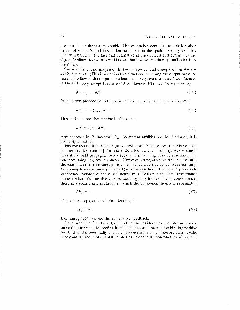
presumed,then the systemis stable.The systemis potentiallyunstablefor othervaluesof a and b, and this is detectablewithin the qualitative physics. Thisfacility is basedon the fact that qualitative physics detectsanddeterminesthesign of feedbackloops. It is well known that positivefeedback(usually) leadstoinstability.

Considerthe causalanalysisof the two narrowconduitexampleof Fig. 4 whena >0, hut /, < 0. (This is a noninuitive situation,as raising the outputpressurelessenstheflow to the output—theload has a negativeresistance.)Confluences(F1)—(F6) apply except that as h <() confluence(F2) must be replacedby

liQ,1151 = —liP,, . (F2’)

Propagationproceedsexactly as in Section 4, except that after step (V5):

liP,, = = — . (V6’)

This indicatespositive feedback.Consider,

lip,,, = liP — liP,, . (F6’)

Any decreasein P,, increasesP,,,. As systemexhibits positive feedback,it isprobably unstable.

Positivefeedbackindicatesnegativeresistance.Negativeresistanceis rareandcounterintuitive (see [4] for more details). Strictly speaking, every causalheuristic should propagatetwo values,one presumingpositive resistanceandone presumingnegativeresistance.However, as negativeresistanceis so rare,thecausalheuristicspresumepositiveresistanceunlessevidenceto thecontrary.Whennegativeresistanceis detected(as is the casehere),the second,previouslysuppressed,version of the causalheuristic is invoked in the samedisturbancecontext where the positive version was originally invoked. As a consequence.thereis a secondinterpretationin which the componentheuristic propagates:

aP,,=— . (V7)

This value propagatesas before leading to

lip,) = + . (V8)

Examining (F6’) we see this is negativefeedback.Thus,whena > 0 andh <0, qualitative physicsidentifIestwo interpretations.

oneexhibiting negativefeedbackandis stable,andthe otherexhibiting positivefeedbackandis potentially unstable.To determinewhich interpretationis validis beyondthe scopeof qualitative physics:it dependsupon whetherV—ab>l.

THEORIESOFCAUSALORDERING 53

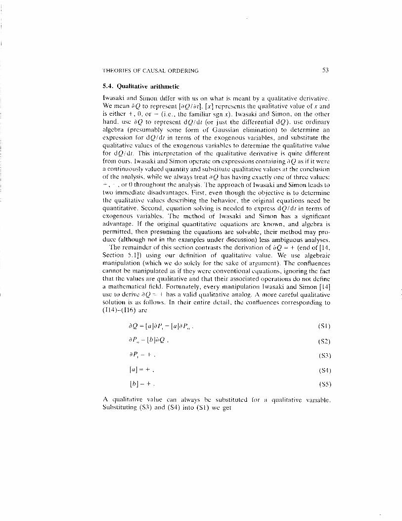
5.4. Qualitative arithmetic

Iwasaki and Simon differ with us on what is meantby a qualitative derivative.We meanliQ to representfaQ/lit]. [x] representsthe qualitativevalueof x andis either +, 0, or — (i.e., the familiar sgnx). Iwasaki andSimon, on the otherhand, use liQ to representdQ/dt (or just the differential dQ), use ordinaryalgebra (presumablysome form of Gaussianelimination) to determineanexpressionfor dQ/dt in terms of the exogenousvariables,and substitutethequalitative valuesof the exogenousvariablesto determinethe qualitativevaluefor dQ/dt. This interpretationof the qualitative derivative is quite differentfrom ours.Iwasaki andSimon operateon expressionscontainingliQ asif it werea continuouslyvaluedquantityandsubstitutequalitativevaluesat the conclusion(If the analysis,while wealwaystreat liQ has having exactlyoneof threevalues:

—, or 0 throughoutthe analysis.The approachof Iwasaki andSimon leadstotwo immediatedisadvantages.First, eventhoughthe objectiveis to determinethe qualitative valuesdescribingthe behavior,the original equationsneedbequantitative. Second,equationsolving is neededto expressdQ/dt in terms ofexogenousvariables. The method of Iwasaki and Simon has a significantadvantage.If the original quantitative equationsare known, and algebra ispermitted, then presumingthe equationsare solvable, their methodmay pro-duce(althoughnot in the examplesunderdiscussion)less ambiguousanalyses.

The remainderof this sectioncontraststhe derivation of liQ = + (endof [14,Section 5.1]) using our definition of qualitative value. We use algebraicmanipulation(which we do solely for the sakeof argument).The confluencescannothe manipulatedas if they wereconventionalequations,ignoringthe factthat the valuesare qualitativeandthat their associatedoperationsdo not definea mathematicalfield. Fortunately,every manipulationIwasaki andSimon [14]use to deriveliQ = + has a valid qualitative analog.A morecarefulqualitativesolution is as follows. In their entire detail, the confluencescorrespondingto(Ii4)—(Il6) are

liQ = [a]liP — [a]liP,, , (Si)

liP,, = [b]aQ (S2)

liP,=+, (S3)

(S4)

(SS)

A qualitative value can always be substituted for a qualitative variable.Substituting(S3) and (S4) into (SI) we get


aQ=[-f-]—aP,,. (S6)

In caseswhere the syntax is potentiallyambiguoussuchasconfluence(S6), thequalitative value + is written as [+]. Substituting(S5) into (S2) we get

liP,,=liQ. (S7)

Generally, equivalentvariables can always be substitutedfor one another.Substituting (S7) into (S6) we get

liQ=[+]—liQ. (S8)

Note that adding liQ to both sides of confluencesproduces:

aQ+aQ=[+]—aQ+aQ. (S9’)

Unfortunately,although[x] + [x] = [xl, [x] — [x] canbe [+], [0] or [—]. AddingliQ to bothsidesof (S8) weakensit so that all solutionsare possible.Insteadwemustuse a generalrule of qualitativealgebrathat [x] = [y] — [x} is true exactlywhen[x] = FyI (provable by case analysis):

aQ=+. (S9)

Conventionalalgebraicmanipulationof expressionswhoseoperationsdo notdefine a field is dangerousbecause many seemingly legal transformationsproduce incorrect results or lose information. For example, given the twoconfluences:

aQ=liP—liP,,, (El)

liP~—liP,,=0, (E2)

it is incorrectto substitute(E2) into (El) to obtain:

aQ=0. (E3)

For example,the assignmentaQ = +, liP~= +, lip,, = + satisfiesconfluences(El) and(E2) but not (E3). This might seemodd, becauseliP — liP,, probablyrepresentsthe samequantityin both(El) and(E2). But this fact is not encodedin confluences (El) and (E2). (The original equations might have beenQ = 2P — P,, and P, — P0 = 0.) To encode the fact that the occurrencesofaP~— liP,, in (El) and (E2) refer to the samevariable one must state thisexplicitly (as in qualitative physics):

THEORIESOF CAUSALORDERING

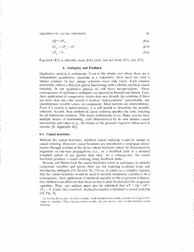
liQ = liP,,, , (E4)

aP,,, = liP,, —- aP, , (ES)

aP,,,=0. (E6)

Equation (E3) is inferable from (E4)—(E6), hut not from (El) and (E2).

6. Ambiguity and Feedback

Qualitative analysisis ambiguous.Even in the simple casewhere there are nindependentquantitative equationsin n unknowns,there need not exist aunique solution. In fact, unique solutions occur only rarely. Each solutionpotentially reflectsa different global functioningwith a distinct mythicalcausalordering. In our qualitative physics we call these interpretations.~Theseconsequencesof qualitative ambiguityare ignored in Iwasaki andSimon. First,their application of comparativestatics doesnot identify the solutions if thereare more than one—thesystemis marked “indeterminate” (presumably.anyunambiguousvariable valuesare computed).Most systemsare indeterminate.Even if a system is indeterminate,it is still useful to determinethe possiblesolutions. Second,their methodof causalorderingspecifiesthe sameorderingfor all behavioralsolutions. This seemsproblematicto us: Many systemshavemultiple modes of functioning, eachcharacterizedby its own distinct causalinteractionsandvalues(e.g.. the modesof the pressureregulatorwhen usedinreverse,[8, Appendix Al).

6.1. Causal heuristics

Without the causal heuristics, mythical causalorderingwould he similar tocausalordering.However,causalheuristicsare introducedto propagatedistur-bancesthroughsectionsof the devicewhosebehaviorcannothe determinedbysequences(If one-step propagations(i.e.. on a feedbackpath or a minimalcomplete subset (If size greater than one). As a consequence,the causalheuristicsproduce a causalorderingalong feedbackpaths.

Iwasaki andSimon treat the causalheuristicssolelyas techniquesto identifyexogenousvariables and ignore their use for ordering feedback loops andintroducingambiguity 114, Section3]). (To us, it comesas a completesurprisethat the causalheuristicswould he usedto identify exogenousvariables.)As aconsequence,their applicationof mythical causalityto the evaporatoris flawed.Our methodis no different than theirsin that it musthe providedthe exogenousvariables. Thus, our analysis must also be informed that aT, = liQ = lip =

a T~= 0. Underthis condition. mythical causalityis identical to causalordering[14, Fig. 3].

‘[4. SectionS[ containsa detailedexample.Eachinterpretationassignsa distinctsetof qualitativevalues to variables. These interpretationsusually, but not always. have distinct mythical causalorderings.


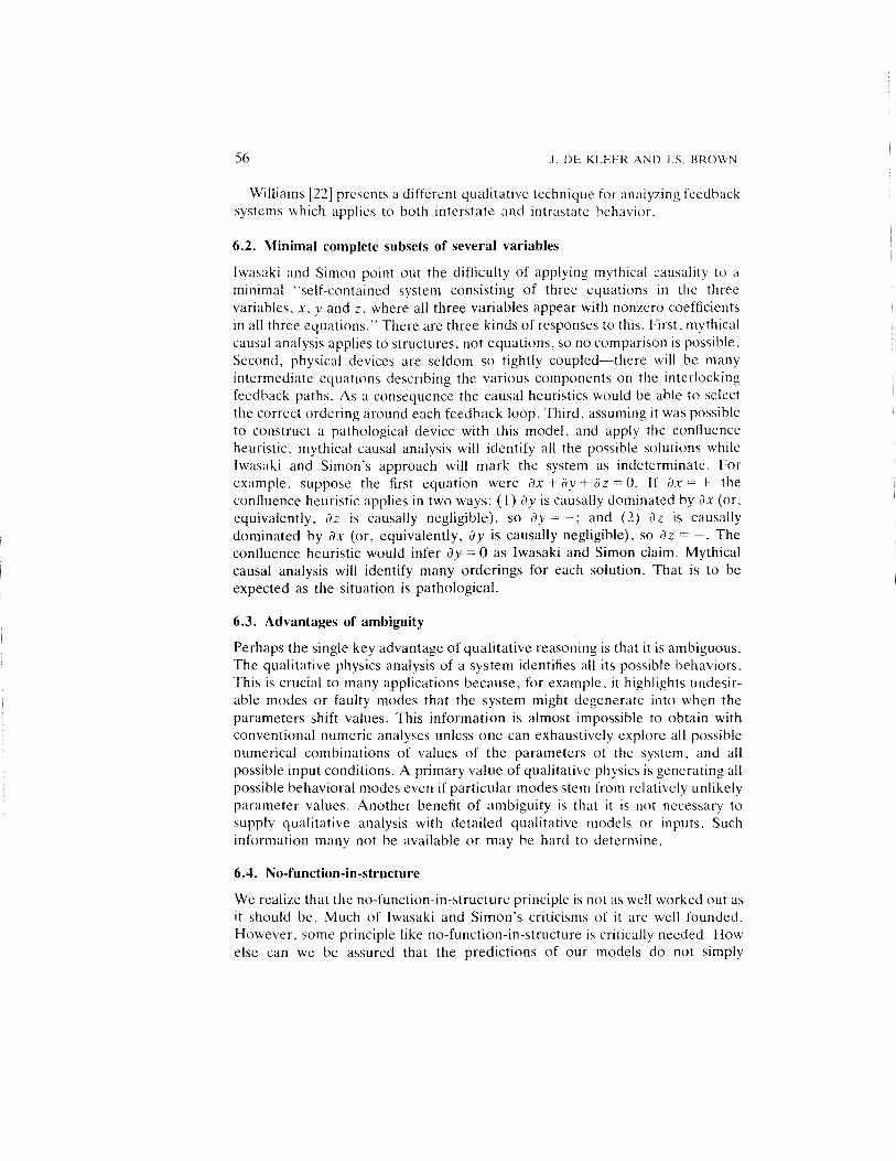
Williams [22] presentsadifferentqualitativetechniquefor analyzingfeedbacksystemswhich applies to both interstateand intrastatebehavior.

6.2. Minimal complete subsetsof several variables

Iwasaki and Simon point out the difficulty of applying mythical causalityto aminimal “self-contained systemconsisting of three equationsin the threevariables,x, y andz, whereall threevariablesappearwith nonzerocoefficientsin all threeequations.”Thereare threekindsof responsesto this. First,mythicalcausalanalysisappliesto structures,not equations,SO no comparisonis possible.Second,physical devicesare seldom so tightly coupled—therewill he manyintermediateequationsdescribingthe various componentson the interlockingfeedbackpaths.As a consequencethe causalheuristicswould he ableto selectthe correctorderingaroundeachfeedbackloop. Third, assumingit waspossibleto constructa pathological device with this model, and apply the confluenceheuristic, mythical causalanalysiswill identify all the possiblesolutions whileIwasaki and Simon’s approachwill mark the system as indeterminate.Forexample, suppose the first equation were lix + liy + liz = 0. If lix = + theconfluenceheuristicappliesin two ways: (1) liy is causallydominatedby lix (or,

equivalently, liz is causally negligible), so liy = —; and (2) liz is causallydominated by lix (or, equivalently, liy is causallynegligible), so liz = —. Theconfluenceheuristicwould infer liy = 0 as Iwasaki and Simon claim. Mythicalcausal analysis will identify many orderings for each solution. That is to beexpectedas the situation is pathological.

6.3. Advantagesof ambiguity

Perhapsthe singlekey advantageof qualitativereasoningis that it is ambiguous.The qualitative physicsanalysisof a systemidentifies all its possiblebehaviors.This is crucial to many applicationsbecause,for example,it highlights undesir-able modesor faulty modes that the systemmight degenerateinto when theparametersshift values. This information is almost impossible to obtain withconventionalnumericanalysesunlessonecan exhaustivelyexploreall possiblenumerical combinationsof values of the parametersof the system, and allpossibleinput conditions.A primary valueof qualitativephysicsis generatingallpossiblebehavioralmodesevenif particularmodesstemfrom relatively unlikelyparametervalues. Another benefit (If ambiguity is that it is not necessarytosupply qualitative analysis with detailed qualitative models or inputs. Suchinformation many not he availableor may he hard to determine.

6.4. No-function-in-structure

We realizethat the no-function-in-structureprinciple is not aswell worked(lut as

it should he. Much of Iwasaki and Simon’s criticisms of it are well founded.However,some principle like no-function-in-structureis critically needed.Howelse can we be assuredthat the predictions of our models do not simply


regurgitateassumptionswe built into them? Will the composition of modelscorrectly characterizethe behaviorof the compositedevice?

Iwasaki and Simon repeatedly criticize the role of the no-function-in-structureprinciple for troubleshooting.

Of course,the assumptionthat a componentis operatingnormallycan fail in the presenceof a malfunction,but in that casethe systemmusthe describedby a new anddifferent set of structuralequations.

Thismissesour point in two ways. First, if the systemis suppliedan unexpectedinput, then the model may predictincorrect behaviorif the componentmodelspresumenormal function, failing to characterizeunusual operating regions.Second,considerthe troubleshootingtask. In troubleshooting,somecomponentis brokencausingits behaviorto deviatefrom its model. As Iwasaki andSimonpoint out, the actualsystemis behavingaccordingto a modifiedset of structuralequations.The task (If troubleshootingis to identify which component isbehavingaccording to a modified model. The standardtroubleshootingap-proachis to reasonbackwardsfrom observationsto determinewhat couldhaveprovokedthe symptom.This backwardsreasoningrequirescorrectcomponentmodels.Considerwhat might happenif no-function-in-structurewereviolated.If A’s (actually unfaulted) componentmodel assumesnormal functioning andthe actually faulted component B forces A into an unusual mode, then both Aand B will appear faulted when, in actuality, only B is. Thus, the violation ofno-function-in-structure in A’s model, makes it impossible to localize the faultto B.

Neither causalorderingnor mythical causalityaddressdirectly theproblemof causalanalysisof a defectivecomponent—i.e.,a compo-nent thatdoesnotobeythe equationsby which it hasbeendescribed.Thatcan he accomplishedonly by redescrihingthe componentin itsfaulty state.

Admittedly, neitherapproachto qualitative reasoningtroubleshootsin itsown right. Qualitativereasoningtechniquesare used as onemodule (If systemachievingsomeothergoal (e.g., troubleshooting).See[1, 2, 101 for examples(If

troubleshootingarchitectureswhich could utilize the predictiveandexplanatorycapabilitiesof a qualitative reasoningsystem. By comparingpredictionswithobservations,they detectsymptoms.They analyzeexplanationsworking back-wardsfrom symptomsto causes.They usethe predictivecapability to evaluatepossiblefaults (by checkingconsistencywith symptoms).To fulfill theseroles,the no-function-in-structureprinciple must he obeyed.

The precedingquote also suggeststhat troubleshootingcan only progresswhenthe faulted componentandits failure modeis known a priori. The wholepoint of troubleshooting is that we do not know what component is faulted orhow it is faulted. The troubleshooting strategiesjust sketchedout do not requirean a priori knowledge about the possiblefaulty behaviors.

Iwasaki and Simon argue that our example (If a light switch illustrates a

58 1. DE KLEER AND iS. BROWN

grain-size issue, not the no-function-in-structureprinciple. We argued that amodel for the light switch which specified no current when off, and nonzerocurrent when on, violated no-function~in-structure.The original light switchmodel presumedit was part (If a normal working light bulb circuit, and thatnonzeropositivecurrent flows when the light switch is on. It is simply not thecasethatcurrentflows through everylight switch whenit is closed.For example.considerhow hard it would he to troubleshoota circuit with a broken light bulb(althoughthe switch is on, we would measureno currentflow, indicating that theswitch violated its behavioralmodel and was faulted). We supplied (personalcommunication)anothermodel in terms (If voltagesand currents,which drewattention to voltagesandcurrentswhich, unfortunately,madethe model changeappearas a grain-size issue. It is an empirical fact that the flow of electricitycannothe modeled(obeyingno-function-in-structure)by a singlevariable type.We neednot call the two variablesvoltageandcurrent: “Stuff” flows throughalight switch only when thereis a sourceof “stuff” (i.e.. availablecurrent) andthereis a pathwayfor this “stuff’’ (i.e., voltage—theelectromotiveforce of thesourcereachesthe switch).

We are notclaimingexperts(Inly usemodelsobeyingno-function-in-structure.Quite the contrary.As is discussedin [71, we claim that expertspossessmultiplemodels, mostof which dramaticallyviolate the no-function-in-structureprin-ciple. But in such casesthe ideal is that the assumptionsincorporatedimplicitlyinto the models that violate no-function-in-structureare explicitly noted ascaveatson the particularmodels. This enablesan expert,or expertsystem,toknow when to exploit a “purer” model, hut one which impcsesan additionalcomputationaltax on the reasoner.

7. Conclusion

We concludeby reviewingthe conclusionof Iwasaki and Simon.

In this paper we have shown how classical methods of causal(Irdering and of comparativestatics are employedto determinethecausalrelationsamongthe variablesandmechanismsthatdescribeadevice, and to assessthe qualitative effectsof disturbancesin thesystemcausedby exogenousvariablesor parameters.Theseproce-dures,which have beenwidely used for more than thirty yearsinseveral fields of science,are generallyconsistentwith, but some-what more general than, the intuitive methods for determiningmythical causationandfor propagatingdisturbancesthat havebeenrecently proposedby de Kleer andBrown. Moreover,they providean explanationof why the intuitive methodswork.

It is unfortunatethat the relationshipbetweencausalorderingandconstraintpropagationwas not recognizedearlier. The ideaof causalorderingcanbenefit

THEORIESOF CAUSALORDERING 59

the propagationof constraintstechniques.However, the techniqueof mythicalcausalityis as preciseas causalorderingandcomparativestatics,producesthesameorder as causalorderingfor nonfeedbacksystems,producescausalordersfor feedback paths, doesnot require knowing the original quantitative equat-ions, does not require any algebraicmanipulation, and works for nonlinearequations.

The methods of causal ordering and comparative statics provide arationalefor the auxiliary assumptionsthat de Kleer andBrown useto guaranteepropagation of disturbances. They are also capableofelucidating causalrelations and qualitative effects in deviceswithfeedback loops, which are handled only with somedifficulty by theintuitive methods.

Until Iwasaki and Simon pointed this out to us we never realized that thecausalheuristicsdetectexogenousvariables.The purposeof thecausalheuristicsis to elucidate causality in feedback loops, which is not possiblewithin theirapproach. Our analysisof the conduit example in Iwasaki and Simon demon-strates how we handle feedback.

We concur fully with de Kleer and Brown that thesemethods (boththe classical and theirs) capture someof the “physical intuition” thathuman beingsare able to apply in reasoningabout physical devices.However, the methods of comparative statics, with their ability tohandle simultaneousrelations,probably go beyond the limits ofunaided human intuition, which seemsmost successfulwhen thecomponents of the systembeing analyzedcan be dealtwith sequen-tially, as they are by the propagationmethod.

We have already argued that mythical causality produces more completecausalorderingthanthe classicalapproachandis specifically designedto handlesimultaneousequations.It has been our experiencethat humansare phenomen-ally good at analyzing nonsequential simultaneoussystems—in terms of feed-back loopswithin the physical structure. This may be the difference betweenaneconomist’sview and an engineer’s. The engineerhaving developedreasoningtechniquesthatexploitphysicalstructurewhile theeconomistdoesnothaveeasyaccessto the structureof the systemshe studies.

When the equilibrium of the systembeing examined represents themaximum or minimum of somefunction, the first-order and second-order conditions for extremaprovide essential information about thesignsof the derivativesthat is invaluablein inferringthe qualitativeeffectsof disturbances.Whenthe equilibrium relationsof a systemcan be derived from dynamic equations, the same kinds of inform-ation are provided by the conditions for dynamicstability.


We concur. However,in many situations,especiallypertainingto engineeredartifacts, the dynamic equationsare unavailable and difficult to obtain orstability can he presumed.

An inference engine capable of the kinds (If formal reasoningdescribedin this paperwould probablyhe a usefuladjunctin manykinds of expertsystems. Building such a systemfrom the specific-ationswe havesketchedhereappearsto be a feasibletask, andit isour intent to undertakesuch a constructionas a next step towardunderstandingqualitative reasoning.

Iwasaki and Simon will find constructingsuch a systema surprisinglydifficulttask. Computing the causalordering is a simple graphsearchand substitutingqualitative variablesinto equationsis straightforward.However, to determinethe derivativesin termsof the exogenousvariablesrequiresalgebraicmanipul-ation. Thesealgebraicmanipulationsare reasonablycomplex: Gaussianelimin-ation with coefficient ratios of multivariate polynomials in the parameters.Computing stability conditions requires evenmore complexsymbolic algebraand will takethe greaterpart of MACSYMA or someequivalentsystem.

We all share the common goal of obtaining a better understandingofqualitative and causal reasoning. It is unfortunate that so many technicalconfusionshave arisen. We failed to appreciatethe importanceof the causalorderingideaof [18]. In turn, Iwasaki andSimon fail to understandthat oneofthe central tenets of our proposalwas to explain feedbackand to develop aqualitative calculusthat sidestepsmany of the difficulties of analyzingdifferen-tial equations(andwhich providessuchadirect connectionbetweenthesolutionmethod and a physical structurethat it becomesa plausible model of humanreasoningaboutphysical systems).We hopethis paperis a steptowardsclearingup thesetechnical misunderstandings.Thesemisunderstandingswill eventuallybe resolved.However, the fundamentaldifferencesbetweenthe approachesofengineeringand economicsis a more serious and interestingquestion. It hasalreadyilluminated qualitativephysics’ intimatedependenceon the structureofa device. It remainsanopenquestionas to what synergyof ideaswill provebestto understandqualitative reasoningin general.

ACKNOWLEDGMENT

We thankDanielG. Bobrow, Ken Forbus,TadHogg,PaulRicci, GerryRoylance,leff Shrager,JohnTukey, Dan Weld. Brian Williams, and Annie Zaenenfor commentingearly draftsand providinginsightful discussions.LenoreJohnsondrew the figures.

Many readers(includingIwasakiandSimon[personalcommunication])pointedoutproblemswiththispaperafterwesentit to IwasakiandSimon.We haveincorporatedsomeof theirclarificationsasfarastheydid not conflict with IwasakiandSimon’sReply. We have profittedgreatly from thepoignantcriticism that Iwasaki andSimonhaveprovided. IncorporatingtheinsightsandclarificationsderivedfromstudyingtheirReplywouldhaveled to amajorrewriteofthispaperwhichneithertime norprotocolpermits.

THEORIES OF CAtJSAL ORDERING 61

REFERENCES

I. Brown. iS.. Burton. R.R. and de Kleer. I., Pedagogical,natural languageand knowledgeengineeringtechniquesin SOPHIE I. II and Ill, in: D. Sleemanand 1.5. Brown (Eds.),Intelligent iutoring S~ferns, (Academic Press,New York, 1982) 227—282.

2. Davis, R.. Shrohe,1-f., Hamscher,W., Wieckert, K.. Shirley, M. andPolit, S.. Diagnosisbasedon description of structure and function, in: Proceedings.Second Conferenceon ArtificialIntelligence,Pittsburgh,PA (1982) 137— 142.

3. de Klcer, I.. Multiple representationsof knowledge in a mechanicsproblem-solver, in:ProceedingsFifth International Joint Confdrenceon Artificial Intelligence, Cambridge. MA(1977) 299—304.

4. de Kleer. i.. How circuits work, Artificial Intelligence24 (1981) 205—280.5. de Kleer. I.. Problemsolving with the ATMS, Artificial Intelligence28 (1986) 197—224.

6. de Kleer. I. and Bobrow, D.G., Higher-orderqualitativederivatives, in: ProceedingsFourthNational (‘onferenceon Artificial Intelligence, Austin, TX (1984) 86—91.

7. de Kleer, J. and Brown, J,S., Assumptionsand ambiguitiesin mechanisticmental models,in: D. Gentner and AL. Stevens(Eds.), Mental Models (Erlbaum, Hillsdale, NJ, 1983)155—190.

8. de Kleer, I. andBrown. IS., A qualitativephysics basedon confluences,Artificial Intelligence24 (1984) 7—83.

9. de Kleer, J. andSussman,G.I., Propagationof constraintsapplied to Circuit synthesis,CircuitTheor. AppI. 8 (1980) 127—144.

10. de Kleer, J. and Williams, B.C., Diagnosingmultiple faults, Artificial Intelligence,submitted.11. Desoer,CA. and Kuh, ES., Basic Circuit Theory (McGraw-Hill, New York, 1969).12. Forbus, K.D., Qualitativeprocesstheory, Artificial Intelligence24 (1984) 85—168.13. Gray, P.E. and Searle,CL., Electronic Principles: Physics,Models, and Circuits (Wiley.

New York, 1969).14. Iwasaki, Y. and Simon, HA., Causality in devicebehavior,Artificial Intelligence29 (1986)

3—32, this issue.15. Kuipers, B., Qualitativesimulation,Artificial Intelligence29 (1986) 289—338,16. Shearer, IL., Murphy, AT. and Richardson, H.H., Introduction to Systetri Dynamics

(Addison-Wesley.Reading,MA, 1971).17. Simon,HA., On the definition of the causalrelation, J. t’hilosophv 49 (1952) 517—528; also:

HA. Simon,Modelsof Discovery(Reidel, Boston, MA, 1977) 86—91.18. Simon,H.A., Causalorderingand identifiability, in: W.C. Hood and T.(’. Koopmans(Eds.).

Studiesin EconometricModels (Wiley, New York, 1953) 49—74; also: H .A. Simon,ModelsofDiscovery(Reidcl, Boston,MA, 1977) 53—70.

19. Stallntan,R. andSussman,G.I., Forwardreasoninganddependency-directedbacktrackingin asystemfor computer-aidedcircuit analysis,Artificial Intelligence9 (1977) 135—196.

20. Steele,G.L.,Thedefinition andimplementationof acomputerprogramminglanguagebasedonconstraints,Al Tech. Rept. 595, MIT, Cambridge,MA, 1979.

21. Sussman,G.I. andSteele,G.L.. CONSTRAINTS—A languagefor expressingalmost-hierar-chical descriptions,Artificial Intelligence14 (1980) 1—39.

22. Williams, B.C., Qualitative analysisof MOS circuits, Artificial Intelligence24 (1984) 281 —346.23. Williams, B.C., ‘T’he useof continuity in a qualitativephysics, in: ProceedingsFourth National

Conferenceon Artificial Intelligence. Austin, TX (1984) 350—354.

ReceivedDecember1985

Documents

Theories of Causal Ordering -