Embed Size (px)
Citation preview

Theoretical treatment of high-frequency,
large-amplitude ac voltammetry applied to ideal
surface-confined redox systems
Christopher G. Bella,1,∗, Costas A. Anastassioub, Danny O’Harea, Kim H.Parkera, Jennifer H. Siggersa
aDepartment of Bioengineering, Imperial College London, South Kensington Campus,
London, SW7 2AZ, UKbDivision of Biology, California Institute of Technology, 91125 Pasadena, California, USA
Abstract
Large-amplitude ac voltammetry, where the applied voltage is a large-amplitudesinusoidal waveform superimposed onto a dc ramp, is a powerful method for in-vestigating the reaction kinetics of surface-confined redox species. Here we con-sider the large-amplitude ac voltammetric current response of a quasi-reversible,ideal, surface-confined redox system, for which the redox reaction is describedby Butler–Volmer theory. We derive an approximate analytical solution, whichis valid whenever the angular frequency of the sine-wave is much larger thanthe rate of the dc ramp and the standard kinetic rate constant of the redoxreaction. We demonstrate how the third harmonic and the initial transient ofthe current response can be used to estimate parameters of the electrochemicalsystem, namely the kinetic rate constant, the electron transfer coefficient, theformal adsorption potential, the initial proportion of oxidised molecules and thelinear double-layer capacitance.
Keywords: ac voltammetry, quasi-reversible, large-amplitude, adsorbed,surface-confined
1. Introduction
Voltammetry has proved to be a very effective technique for probing the elec-trochemical properties of adsorbed redox species, [1–18]. The technique consistsof applying a voltage to an electrode on which the molecules are adsorbed andanalysing the form of the resultant current response to obtain information aboutthe parameters driving the underlying redox reaction. The most commonly usedtechnique has been cyclic voltammetry, although more recently there has been
∗Corresponding authorEmail address: [email protected] (Christopher G. Bell)
1Tel: +44 207 594 7419, Fax: +44 207 594 9817
Preprint submitted to Elsevier November 10, 2011

interest in the application of large-amplitude ac voltammetric techniques, wherethe applied voltage consists of dc ramp with either a large-amplitude sine-wave,[19–25], or a large-amplitude square-wave, [26–29], superimposed onto it.
One difficulty encountered with traditional techniques such as cyclic voltam-metry and small-amplitude ac voltammetry is that the current response is con-taminated by a charging current due to double-layer capacitance; this obscuresthe faradaic current that contains the information relevant to the electron trans-fer process. Isolation of the faradaic current response is difficult and is usuallyachieved by using inexact techniques such as background subtraction for cyclicvoltammetry, and equivalent circuit analysis for small-amplitude ac voltamme-try. Background subtraction is particularly likely to be inaccurate for adsorbedredox molecules, since the adsorption of the molecules will substantially changethe nature of the electrical double-layer. This difficulty in removing the charg-ing current is one of the reasons for the increasing interest in large-amplitudeac voltammetry (e.g. see the discussion in the article by Bond et al. [30]), whichallows purely faradaic information to be extracted directly from the experi-ment, without having to resort to any potentially inaccurate techniques for theremoval of the charging current. Use of a large-amplitude excitation exploitsthe non-linearity of the current response to increase the magnitude of the higherharmonics, and extraction of these higher harmonics using the FFT provides ac-cess to a wealth of purely faradaic information, since double-layer capacitanceeffects are confined to the lower harmonics.2
Interpretation of the current response from a voltammetric experiment isgreatly aided by theoretical models. Laviron [31] pioneered theoretical mod-elling of the voltammetric responses of surface-confined systems, including ananalytical solution for the current response to a linear potential sweep input,[32], and investigations into the faradaic impedance of a small-amplitude ac po-larographic experiment, [33–35]. Other theoretical work on linear sweep/cyclicvoltammetry includes that by Weber and Creager [36], Honeychurch [37] andMyland and Oldham [38]; further theoretical investigations into the interpre-tation of the current response of small-amplitude ac voltammetric experimentshave been performed by Creager and Wooster [39], Yap [40] and Harrington[41].
Theoretical research to improve our understanding of the current responseof large-amplitude sinusoidal ac voltammetry of surface-confined systems hasinvolved a number of approaches. Harrington, [42], derived a system of infi-nite equations to be solved for the harmonic amplitudes of the quasi-reversiblecurrent response when the dc ramp is zero. Honeychurch and Bond [43] al-lowed the dc ramp to be non-zero and developed numerical simulations for thecurrent response; they also derived an analytical solution for harmonics of thecurrent response produced by a reversible redox reaction (valid for excitation
2We note that other effects such as ohmic drop can also contaminate the information con-tained in the higher harmonics, and we discuss practical ways of dealing with this later in thearticle, in Section 3.4.
2
amplitudes up to ≈65mV). Guo et al. [20] presented an analysis of numericalsimulations of quasi-reversible reactions, and discussed the application of thetechnique to an adsorbed azurin thin film. Fleming et al. [22] investigated theinclusion of the effects of uncompensated resistance into the numerical simula-tions. Anastassiou et al. [21] discussed how the Hilbert transform could be usedto interpret the current response rather than using the FFT. Finally, we haverecently published an article [44] in which we found an approximate analyticalsolution for the large-amplitude current response of a quasi-reversible system,when the dc ramp is zero and the frequency of the sinusoidal excitation is high.
In this article we investigate analytically the current response of surface-confined species to large-amplitude ac voltammetry when the dc ramp is non-zero. Inclusion of a non-zero dc ramp has the benefit that the entire potentialwindow can be scanned, in theory providing more information in the harmonicsof the current response. As in our previous article [44], we assume that thesurface-confined system is ideal and that the redox reaction is quasi-reversiblewith kinetics described by Butler–Volmer theory, [45]. Using the asymptotictechnique of multiple scales [46], we derive a novel analytical solution for thecurrent response that is valid whenever the frequency of the sine-wave is muchlarger than both the kinetic rate constant of the redox reaction and the rate ofthe dc ramp. We find analytical solutions for the time-dependent envelopes ofthe harmonics and we demonstrate how the envelope of the third harmonic canbe used to estimate the Butler–Volmer parameters of the redox reaction, namelythe standard kinetic rate constant, k0, the electron transfer coefficient, α, andthe formal adsorption potential, E0′
a . The analytical expression for the envelopeis a function of k0, α and E0′
a , and estimates for their values can be found byfitting this function (using a non-linear curve-fitting procedure) to the envelopeextracted from the experimental current response using the FFT. Finally wedemonstrate how the initial proportion of oxidised molecules, θ, and the lineardouble-layer capacitance, Cdl, can be estimated from the initial transient partof the current response.
2. Theory
2.1. Description of the problem
We assume that two redox species, Ox and Red, with surface concentrationsΓO(t) and ΓR(t) (mol m−2) are ideally adsorbed onto an electrode surface (tildesin this article denote dimensional variables). The conditions for ideal adsorptionare detailed in [31, 47, 48]. The redox reaction is such that n electrons areexchanged with the electrode, with the direction of the exchange dependent onthe level of the applied potential, E(t) (V):
Ox + nekf (t)⇋
kb(t)Red. (1)
If the molecules of the redox species are ideally adsorbed according to a Lang-muir isotherm, then we can use Butler–Volmer-type expressions to write the
3
forward and backward rate constants, kf (t) and kb(t), in terms of the applied
potential, E(t):
kf (t) = k0 exp
(
−αnF
RT(E(t)− E0′
a )
)
, (2)
kb(t) = k0 exp
(
(1− α)nF
RT(E(t)− E0′
a )
)
, (3)
where the adsorption formal potential, E0′
a (V), is defined by:
E0′
a = E0 −RT
nFlog
(
bO
bR
)
, (4)
and bO and bR (m3 mol−1) are the Langmuir isotherm adsorption coefficientsfor the oxidant and the reductant, assumed to be either potential-independentor identical functions of the potential [31]. The other parameters follow theusual Butler–Volmer formalism, so that α (0 ≤ α ≤ 1) is the electron transfercoefficient, k0 (s−1) is the standard kinetic rate constant, and E0 (V) is theformal oxidation potential. The remaining parameters are Faraday’s constantF (96,485 C mol−1), the universal gas constant R (8.3145 C V mol−1 K−1),and the temperature T (K), normally taken to be standard room temperature298.15 K.
For ac voltammetry, the applied voltage E(t) consists of a sinusoidal signalsuperimposed onto a dc ramp:
E(t) = Ein + vt+∆E sin(ωt). (5)
Here Ein (V) is the initial starting voltage, v (V s−1) is the dc ramp, ∆E (V) isthe amplitude of the sinusoidal signal and ω (rad s−1) is its angular frequency.Throughout this article we assume that v > 0, so that the oxidation reactionbecomes more important as time progresses; similar analysis will apply for v < 0.
The redox reaction at the surface is modelled by the following ODE’s:
dΓO
dt= kb(t)ΓR(t)− kf (t)ΓO(t), (6)
dΓR
dt= −kb(t)ΓR(t) + kf (t)ΓO(t), (7)
so that matter is conserved as the reaction progresses, and:
ΓO(t) + ΓR(t) = ΓT, (8)
where ΓT (mol m−2) is the constant aggregate surface concentration of theadsorbed species. Initially we assume that surface concentration contains amixture of molecules in both the oxidised and reduced states; we define the
4

initial proportion of molecules in the oxidised state to be 0 ≤ θ ≤ 1, so that
ΓO(0) = θΓT , ΓR(0) = (1− θ)ΓT. (9)
The faradaic current response, i(t) (A), resulting from the redox reactiondepends on the rate of change of concentration of the oxidised species:
i(t) = nF AdΓO
dt, (10)
where A (m2) is the area of the electrode.Using (8) to eliminate ΓR, equation (6) can be written solely in terms of ΓO:
dΓO
dt+(
kf (t) + kb(t))
ΓO(t) = kb(t)ΓT , (11)
which is solved with the initial condition given by ΓO(0) = θΓT. Note that onceΓO(t) has been found, it is easy to find ΓR(t) from (8).
To solve the problem, we first use the following scalings to non-dimensionalise:
t =
(
RT
nF v
)
t, ΓO = ΓTΓ, (12)
E0 =RT
nFE0, E(t) =
RT
nFE(t), (13)
i(t) =
(
(nF )2AΓT v
RT
)
i(t). (14)
We have chosen to scale time with the time-scale of the dc ramp. In the non-dimensional variables, the problem becomes:
dΓ
dt+ µg(t)Γ(t) = µh(t), (15)
with initial condition Γ(0) = θ. Here the functions g(t) and h(t) are given by:
g(t) = e(1−α)(η+t)e(1−α)∆E sin ζt + e−α(η+t)e−α∆E sin ζt, (16)
h(t) = e(1−α)(η+t)e(1−α)∆E sin ζt, (17)
whereη = Ein − E0′
a , (18)
and the non-dimensional parameters ζ and µ, which can be considered as thenon-dimensional frequency and rate constant respectively, are given by
ζ =RT ω
nF v, µ =
RT k0
nF v. (19)
5

The formal solution to this initial value problem is:
Γ(t) = θ exp
(
−µ
∫ t
0
g(u) du
)
+
µ
∫ t
0
exp
(
−µ
[∫ t
0
g(u) du−
∫ s
0
g(u) du
])
h(s) ds. (20)
The faradaic current response is given by i(t) = dΓ/dt, which can also be writtenfrom (15) as:
i(t) = µh(t)− µg(t)Γ(t). (21)
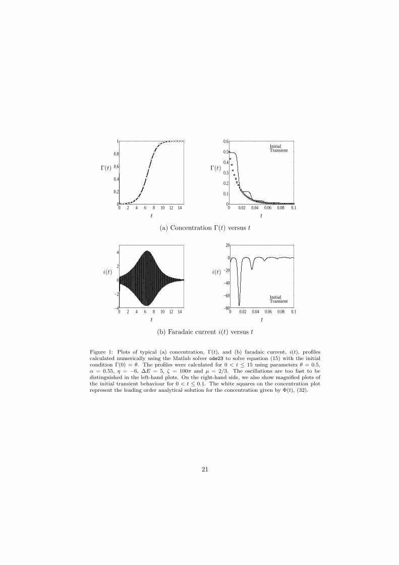
Although the expressions (20) and (21) can be used to calculate concentrationand current profiles using numerical quadrature routines, we found that it waseasier to solve the initial value problem given by equation (15) and initial condi-tion Γ(0) = θ directly. Using the Matlab numerical solver ode23, we calculatedtypical concentration and current profiles for the time range 0 < t ≤ 15 usingthe parameters θ = 0.5, α = 0.55, η = −6, ∆E = 5, ζ = 100π, and µ = 2/3.The profiles are shown in Figure 1 and have been sampled at a rate of 100 pointsper cycle of the voltage excitation.
2.2. Approximate analytical solution for the faradaic current at high frequencies
It is difficult to understand how the faradaic currrent response depends onthe underlying parameters of the electrochemical system from the formal ana-lytical solutions for the concentration and the current, (20) and (21). To gainmore insight, we assume that both ζ−1 ≪ 1 and µζ−1 ≪ 1, which, from (19),corresponds to
RT ω
nF v≫ 1,
ω
k0≫ 1, (22)
so that the angular frequency of the sinusoidal excitation is much larger thanthe rate of the dc ramp and the kinetic rate constant of the redox reaction.
The solution then lends itself to the asymptotic technique of multiple scales,[46]. Let us define two timescales:
τ1 = t, τ2 = ζt. (23)
ThendΓ
dt=
∂Γ
∂τ1+ ζ
∂Γ
∂τ2, (24)
where ζ ≫ 1. Hence the governing equation (15) becomes:
∂Γ
∂τ2+ ζ−1 ∂Γ
∂τ1= −µζ−1g(τ1, τ2)Γ(τ1, τ2) + µζ−1h(τ1, τ2). (25)
We expand Γ(τ1, τ2) in a perturbation expansion in ζ−1:
Γ(τ1, τ2) = Γ0(τ1, τ2) + ζ−1Γ1(τ1, τ2) + ζ−2Γ2(τ1, τ2) + . . . . (26)
6

Then, to leading order, equation (25) is:
∂Γ0
∂τ2= 0, (27)
with initial condition Γ0(0, 0) = θ. This has solution:
Γ0(τ1, τ2) = Φ(τ1), where Φ(0) = θ. (28)
The function Φ(τ1) is determined by considering the secular terms in the O(ζ−1)equation, which is:
∂Γ1
∂τ2+
dΦ
dτ1= −µg(τ1, τ2)Φ(τ1) + µh(τ1, τ2). (29)
Note that the solutions for Γ1 and Φ(τ1) will be valid for any µ such thatµζ−1 ≪ 1.
Next we expand the exponentials with trigonometric exponents in g(τ1, τ2)and h(τ1, τ2), (16) and (17), in terms of the following modified Bessel functionexpansion [49], (p376, 9.6.35):
ez sin τ2 = I0(z)− 2
∞∑
m=1
(−1)m{
I2m−1(z) sin(
(2m− 1)τ2)
− I2k(z) cos(
2mτ2)}
,
(30)where either we set z = (1 − α)∆E or z = −α∆E. This expansion holds for∆E of any size, so that this theory is valid for large-amplitude ac voltammetry.Substituting these expansions into (29), we find that, to remove the secular(growing) terms, Φ(τ1) must satisfy:
dΦ
dτ1= −µ
(
I0(
(1− α)∆E)
e(1−α)(η+τ1) + I0(
− α∆E)
e−α(η+τ1))
Φ(τ1)
+ µI0(
(1− α)∆E)
e(1−α)(η+τ1), (31)
with initial condition Φ(0) = θ. We split the solution for Φ(τ1) into two parts:the initial transient, Φi(τ1), which depends on the initial condition θ, and Φo(τ1),which is independent of the initial condition. The solution is therefore given by:
Φ(τ1) = Φi(τ1) + Φo(τ1), (32)
where
Φi(τ1) = θe−Ψ(τ1)+Ψ(0), (33)
Φo(τ1) = µI0(
(1− α)∆E)
∫ τ1
0
eΨ(z)−Ψ(τ1)e(1−α)(η+z) dz, (34)
7

and
Ψ(τ1) =µI0(
(1− α)∆E)
(1− α)e(1−α)(η+τ1) −
µI0(α∆E)
αe−α(η+τ1). (35)
Note that Ψ(τ1) − Ψ(0) ≥ 0 and increases exponentially as τ1 increases, andhence that Φi(τ1) decays monotonically from θ to zero.
In terms of t, the concentration is given from (28) by
Γ(t) = Φ(t) +O(ζ−1, µζ−1), (36)
and it tends to 1 as t → ∞. The current is given by:
i(τ1, τ2) =∂Γ0
∂τ1+
∂Γ1
∂τ2+O(ζ−1, µζ−1), (37)
which can be written from (28) and (29) as:
i(τ1, τ2) = −µg(τ1, τ2)Φ(τ1) + µh(τ1, τ2) + O(ζ−1, µζ−1). (38)
Substituting for g(t) and h(t) from (16) and (17), and using (30), the leadingorder current (38) can be written as
i(τ1, τ2) = idc(τ1) +
∞∑
m=1
A2m−1(τ1) sin(
(2m− 1)τ2)
+
∞∑
m=1
A2m(τ1) cos(
2mτ2)
+O(ζ−1, µζ−1), (39)
or in terms of t,
i(t) = idc(t) +
∞∑
m=1
A2m−1(t) sin(
(2m− 1)ζt)
+
∞∑
m=1
A2m(t) cos(
2mζt)
+O(ζ−1, µζ−1). (40)
The current is the sum of a dc term, idc(t), and an infinite sum of harmonics.The dc term has the form:
idc(t) = µ
[
e(1−α)(η+t)I0(
(1−α)∆E)(
1−Φ(t))
− e−α(η+t)I0(
α∆E)
Φ(t)
]
, (41)
8
while the time-dependent coefficients of the harmonics, Am(t), are given by:
Am(t) = 2µ(−1)m+m+mod(m, 2)2
[
e(1−α)(η+t)Im(
(1 − α)∆E)(
1− Φ(t))
+ (−1)m+1e−α(η+t)Im(
α∆E)
Φ(t)
]
, m = 1, 2, 3, . . . , (42)
where ‘mod(m, 2)’ gives the remainder on division of m by 2. The envelopes ofthe harmonics are given by
A±
m(t) = ±2µ
[
e(1−α)(η+t)Im(
(1− α)∆E)(
1− Φ(t))
+ (−1)m+1e−α(η+t)Im(
α∆E)
Φ(t)
]
+O(ζ−1, µζ−1),
m = 1, 2, 3, . . . . (43)
After the initial transient has disappeared, the envelopes can be written in termsof Φo(t), (34), so that:
A±
m, o(t) = ±2µ
[
e(1−α)(η+t)Im(
(1− α)∆E)(
1− Φo(t))
+ (−1)m+1e−α(η+t)Im(
α∆E)
Φo(t)
]
+O(ζ−1, µζ−1),
m = 1, 2, 3, . . . , (44)
and they have no dependence on the initial condition θ. Note that, since 0 <Φo(t) < 1, if m is odd, then the two terms in the square bracket have the samesign and combine to give a larger amplitude, whereas if m is even, then theyhave opposite signs, and will tend to offset one another. This results in the evenharmonics having smaller amplitudes than the odd harmonics, so that they areless useful for analytic purposes, as the asymptotic error is relatively larger.
2.3. Charging current due to double-layer capacitance
In addition to the faradaic current discussed in the previous sections, therewill also be a charging current due to the double-layer capacitance at the elec-trode surface. It is usually assumed that this current is independent of thefaradaic current and that the total current, itot(t), is simply a sum of both thefaradaic, i(t) (given by (10)), and double-layer capacitance, idl(t), components,i.e.
itot(t) = i(t) + idl(t). (45)
9
The simplest model for idl(t) assumes that the double-layer is a linear capacitorwith constant capacitance per unit area, Cdl (F m−2), so that:
idl(t) = CdlAdE(t)
dt= CdlAv + ωCdlA∆E cos(ωt). (46)
Hence, in this model, the double-layer current contributes only to the dc com-ponent and the fundamental harmonic of the current reponse, leaving the higherharmonics free of capacitive effects. In non-dimensional terms, the double-layercurrent, idl(t), has the form:
idl(t) = C
(
1 + ζ∆E cos(ζt))
, (47)
where the non-dimensional parameter, C, measures the size of the capacitanceand is given by
C =CdlRT
(nF )2ΓT
. (48)
Note that if ζ ≫ 1, as we have assumed in the previous section, then (47) indi-cates that the contribution of the charging current to the fundamental harmonicis likely to dominate the faradaic component (unless C = O(ζ−1)).
3. Results and discussion
Firstly we validate our analytical results by comparison to a numericallycalculated solution, and secondly we discuss how the analytical solution canbe used to estimate the parameters describing the redox reaction from an ex-perimental current response. Finally, we discuss practical considerations foreffective implementation of the technique.
3.1. Comparison of asymptotic solution to a numerically calculated current
To verify the asymptotic solution, we use the numerical solution plotted inFigure 1 for the parameters θ = 0.5, α = 0.55, η = −6, ∆E = 5, ζ = 100π andµ = 2/3. Since ζ−1, µζ−1 ≪ 1, the numerical solution satisfies the conditions forthe asymptotic solutions for the concentration, (36), and the faradaic current,(40), to be valid. For these values of ζ and µ, the percentage error in theasymptotic solution is O(0.3%).
The profile of the concentration, Γ(t), is plotted as a solid line in Figure 1(a), with the initial transient magnified in the right-hand plot. The leading-order asymptotic solution given by (36) is shown as white squares. The agree-ment between the numerical and analytical solutions is excellent after the initialtransient has disappeared; however, the agreement is not as good in the initialtransient region, when the concentration declines steeply to zero. To reduce theerror in this region, the frequency must be increased. Figure 2 (a) shows thetransient concentration with the frequency increased to ζ = 1000π; the agree-ment between the analytical and numerical solutions improves substantially.
10

This indicates that if the analytical solution is to be used to extract infor-mation from the initial transient, then the experiment must be run at higherfrequencies than is required to extract information from the non-transient partof the current response.
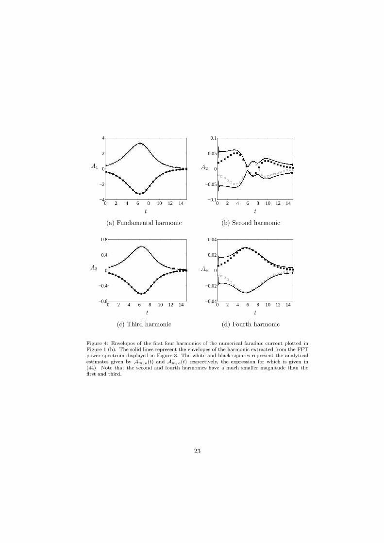
To investigate the accuracy of the asymptotic solution for the faradaic cur-rent, (40), we compare the analytical solution for the envelopes of the harmonicsafter the initial transient has disappeared, (44), to those extracted from the nu-merical current plotted in Figure 1 (b) using the FFT, [50]. We took the FFT ofthe numerical current over the time interval [0.2, 15], thus avoiding any effectsof the initial transient, and the power spectrum is shown in Figure 3. The peaksof the different harmonics are well-separated, despite their coefficients Am(t) be-ing time-dependent; the reason for this is that ζ is large. As expected from thediscussion at the end of Section 2.2, the peaks for the even harmonics are muchsmaller than those for the odd harmonics, since they have smaller amplitudes.Isolating each peak and inverting the FFT gives the harmonics as a function oftime. The envelopes for each harmonic were obtained by finding the maximaand minima, and this gave the results shown in Figure 4 for the first four har-monics. The agreement with the analytical estimates (44) is excellent for theodd harmonics, but less good for the even harmonics, since their magnitude issmall and the asymptotic error is relatively larger.
As we detail below, information from the dc part of the total current response(including both faradaic and capacitive components) in the initial transientregion can be used to estimate the initial proportion of oxidised molecules, θ,and the linear capacitance, Cdl. This information can be obtained by integratingthe current over a moving window of an integer, p, number of periods of thesinusoidal excitation, [t1, t1 + 2pπ/ζ]. This shifts the effect of the harmonicsto higher order and removes any periodic components of the current due todouble-layer capacitance, thus leaving purely dc information from which θ andCdl can be estimated. In non-dimensional terms, we write the integral of thecurrent as follows:
Itot(t1, p) =ζ
2pπ
∫ t1+2pπ/ζ
t1
itot(t) dt, (49)
where itot(t) is the linear sum of the faradaic current and the current due todouble-layer capacitance. Substitution of the approximate analytical solution(40) for the faradaic current, i(t), and the expression for the current due to thedouble-layer capacitance, idl(t), given by (47), into this integral gives:
Itot(t1, p) = Idc(t1, p) + C+O(ζ−1, µζ−1), (50)
where Idc(t1, p) is given by:
Idc(t1, p) =ζ
2pπ
∫ t1+2pπ/ζ
t1
idc(t) dt, (51)
11
and is the integral of the dc part of the faradaic current response, idc(t), theanalytical expression for which is given by (41).
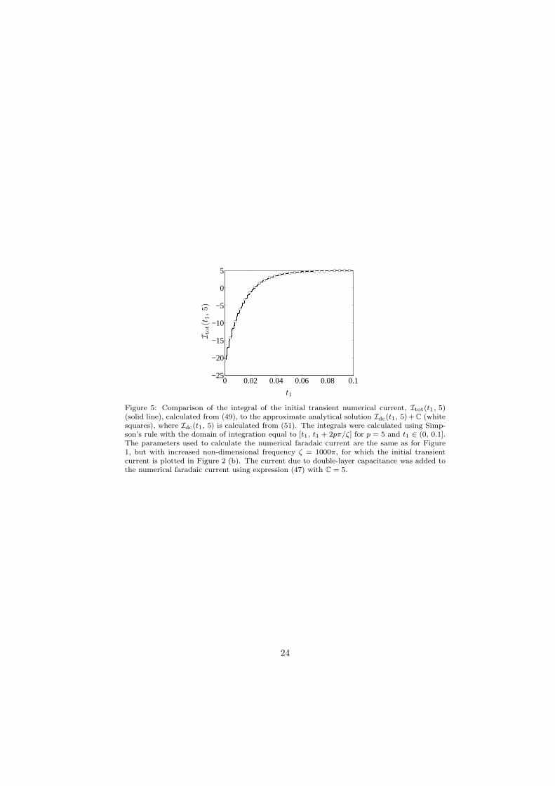
To demonstrate that Idc(t1, p) + C is a good approximation to Itot(t1, p)in the initial transient region of the current response, we calculated Itot(t1, p)from the sum of the numerical transient faradaic current plotted in Figure 2(b) (for the higher frequency ζ = 1000π) and the capacitive current determinedfrom expression (47) with C = 5. The integral Idc(t1, p) was calculated us-ing the analytical expression (41) for idc(t). We chose the parameters p = 5and t1 ∈ (0, 0.1], and both integrals were calculated using Simpson’s rule. Thecomparison is shown in Figure 5, where Itot(t1, p) is shown as a solid line andIdc(t1, p) + C as white squares; the agreement is excellent. Note that, in prac-tice, the appearance of oscillations in Itot(t1, p) will be a good indication thatthe experimental frequency is not high enough for the approximate analyticalintegral to be valid.
3.2. Estimation of system parameters
The purpose of an ac voltammetric experiment is to extract informationabout the underlying electrochemical processes. In the Butler–Volmer formal-ism, this translates into being able to estimate the system parameters from thecurrent response, namely the electron transfer coefficient, α, the formal adsorp-tion potential, E0′
a , the kinetic rate constant, k0, and the initial proportionof molecules in the oxidised state, θ. We also show how to estimate the lin-ear double-layer capacitance, Cdl. We assume that the total concentration ofmolecules, ΓT , the area of the electrode, A, and the number of electrons trans-ferred, n, are known.
The total concentration of molecules, ΓT , is usually determined from the areaunder the peak of a dc cyclic voltammetry experiment undertaken at a very slowscan rate to minimise the effects of double-layer capacitance, cf. [28]. At firstglance, this seems to negate the advantages of ac voltammetry, if one of the pa-rameters has to be determined using cyclic voltammetry. However, calculation
of ΓT does not suffer from the usual disadvantages of cyclic voltammetry, sincethe experiment is conducted at scan rates slow enough to ensure that capacitiveeffects are negligible and that background subtraction is not required. However,slow scan rates do not permit the extraction of kinetic information, and, atfaster scan rates, ac voltammetry is a more effective investigative technique.
3.2.1. Estimation of α, E0′
a and k0 from the harmonic envelopes
In dimensional terms, the envelopes of the harmonics after the initial tran-sient has disappeared can be derived from (44) to give the following leadingorder expression:
A±
m, o(t) ≈ ±2nF AΓT k0
[
e(1−α)f(η+vt)Im(
(1 − α)f∆E)(
1− Φo(f vt))
+ (−1)m+1e−αf(η+vt)Im(
αf∆E)
Φo(f vt)
]
, (52)
12

where f = nF/RT and η = Ein − E0′
a . In terms of the dimensional variables,Φo(f vt), (34), is given by
Φo(f vt) = k0I0(
(1 − α)f∆E)
∫ t
0
eΨ(f vz)−Ψ(f vt)e(1−α)f(η+vz) dz, (53)
and Ψ(f vt), (35), by
Ψ(f vt) =
(
k0
f v
)[
I0(
(1 − α)f∆E)
(1− α)e(1−α)f(η+vt) −
I0(
− αf∆E)
αe−αf(η+vt)
]
.
(54)The expression for A±
m, o(t), (52), is a highly non-linear function of the unknown
parameters k0, E0′
a and α. Since we are using information after the initialtransient has disappeared, the envelopes have no dependence on the unknowninitial condition, Γ(0) = θΓT. Unlike sinusoidal voltammetry, [44], it is notpossible to obtain simple algebraic formulae to estimate the parameters, andwe proceed by fitting this analytical expression to the experimental harmonicenvelopes using non-linear optimisation.
The envelopes of the mth experimental harmonic are found by extracting themaxima and minima of the harmonic obtained using the FFT, which we shallrepresent by (tj , Xj) and (tk, Xk) respectively. To estimate α, k0 and E0′
a fromthe mth harmonic requires finding the values that minimise the following leastsquares objective functions. Firstly, using the maxima, the following functionshould be minimised:
Fmax,m(α, k0, E0′
a ) =∑
j
(
|A±
m, o(tj)| − |Xj |)2
, (55)
and for the minima
Fmin,m(α, k0, E0′
a ) =∑
k
(
|A±
m, o(tk)| − |Xk|)2
. (56)
Both minimisations should give similar estimates for the parameters, and theaverage can be used as a final estimate.
The odd harmonics should be used in these functions, since the even har-monics have smaller amplitudes, and are therefore more prone to experimentaland asymptotic error; we recommend using the third harmonic, as the funda-mental harmonic is likely to include unwanted double-layer capacitance effects,as discussed in Section 2.3. The non-dimensional expression for the double-layer charging current, (47), indicates that its contribution to the fundamentalharmonic is likely to be large. This can result in spectral leakage from the fun-damental harmonic in the power spectrum of the FFT, which causes difficultiesin isolating the peak due to the third harmonic. In this case, the Hann window[51] can be used to reduce the spectral leakage and enable the harmonic to beextracted cleanly (as explained in our previous articles [44, 52, 53]).
13

3.2.2. Estimation of θ and Cdl from the initial transient
Estimates of the initial proportion of oxidised molecules, θ, and the linearcapacitance, Cdl, can be found by using information from the initial transient ofthe current response. This can be achieved by integrating the current responseover a moving window of an integer, p, number of periods of the sinusoidalexcitation, [t1, t1 + 2pπ/ω], as described in the last part of Section 3.1. Thisgives the following function:
Itot(t1, p) =ω
2pπ
∫ t1+2pπ/ω
t1
itot(t) dt. (57)
Re-dimensionalising expression (50) in Section 3.1 shows that Itot(t1, p) is ap-proximated by the following analytical formula for high frequencies:
Itot(t1, p) ≈ Idc(t1, p) + CdlAv, (58)
where
Idc(t1, p) =AΓT (nF )2vω
RT2pπ
∫ t1+2pπ/ω
t1
idc(f vt) dt. (59)
Here, as before, f = nF/RT , and idc(f vt) can be written using (41) in termsof the dimensional parameters as:
idc(f vt) =
(
k0
f v
)
[
e(1−α)f(η+vt)I0(
(1− α)f∆E)(
1− Φ(f vt))
− e−αf(η+vt)I0(
αf∆E)
Φ(f vt)
]
, (60)
where η = Ein − E0′
a and Φ(f vt) = Φi(f vt) + Φo(f vt). Here Φo(f vt) is givenby (53), and Φi(f vt) can be written from (33) as:
Φi(f vt) = θe−Ψ(f vt)+Ψ(0), (61)
where Ψ(f vt) is given by (54).If α, k0 and E0′
a have been determined from the third harmonic, then theonly unknown parameters in (58) are θ and Cdl, which can then be estimatedby finding the values that give the best least squares fit of Idc(t1, p)+ CdlAv toItot(t1, p) over a range of t1 encompassing the initial transient.
3.3. Illustration of estimation of parameters
To illustrate the procedure for estimating the unknown parameters detailedin the previous section, we use the non-dimensional numerically calculated cur-rents. Firstly we use the faradaic current plotted in Figure 1 (b) for ζ = 100πto estimate µ(= 2/3), α(= 0.55) and η(= −6) from the envelopes of the thirdharmonic. Next we use the higher frequency initial transient current plotted in
14

Figure 2 (b) for ζ = 1000π, with the current due to double-layer capacitanceadded using expression (47) with C = 5, to estimate θ(= 0.5) and C. This is thenon-dimensional equivalent of finding the parameters k0, α, E
0′
a , θ and Cdl fromactual experiments. In practice it will be possible to obtain all the parametersfrom a single experiment, as long as the experimental frequency is high enoughto extract the transient information accurately.
The envelopes of the third harmonic after the initial transient has disap-peared were found using the FFT as described in Section 3.1. Then we usedthe Matlab function lsqcurvefit to fit the function A±
3, o(t), (44), to the twoenvelopes given by the maxima and minima, which are displayed in Figure 4(c). Averaging the estimates for µ, α and η given by each fitting procedure, wedetermined accurate estimates of µ ≈ 0.6660, α ≈ 0.5512 and η ≈ −5.9969.
Then, to estimate θ and C from the initial transient current, we used thesevalues for µ, α and η and fitted Idc(t1, p)+C, where Idc(t1, p) is given by (51),for p = 5 and t1 ∈ (0, 0.1] to Itot(t1, 5) (plotted in Figure 5 as the solid line), alsousing the Matlab function lsqcurvefit. This gave estimates of θ ≈ 0.5157 andC ≈ 4.9773. The accuracy of the estimate for θ can be improved by increasingthe frequency of the applied sinusoidal excitation. Increasing the frequencyimproves the resolution of the doubly exponential decay of the transient, ascan be seen by comparison of the transient currents in Figures 1 (b) and 2 (b);the shape of the transient becomes much more apparent when the frequency isincreased from 100π to 1000π.
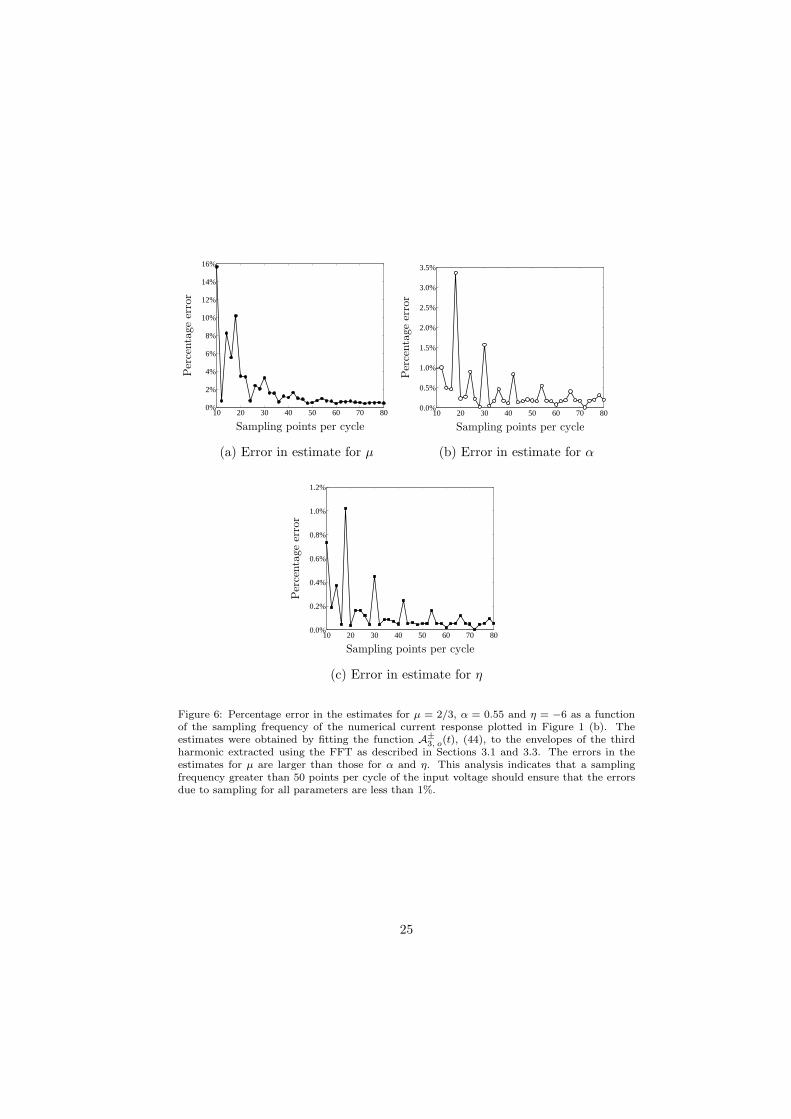
The numerical currents used to calculate these estimates (both for ζ = 100πand ζ = 1000π) were sampled at a high sampling rate of 100 points per cycleof the input voltage, so we also investigated the effect of reducing the samplingrate on the accuracy of the estimates. The percentage errors in the estimatesfor µ, α and η are plotted in Figure 6 (a)–(c) as a function of the number ofsampling points per cycle, which we varied from 10 to 80. The errors in theestimate for µ are greater than those for α and η. In dimensional terms, thissuggests that the estimates for α and E0′
a are likely to be more accurate thanthose for k0 unless the sampling frequency is high enough. The analysis alsoindicates that the sampling frequency should be above 50 points per cycle ofthe input voltage to ensure that the errors due to sampling in the estimates ofthe parameters are less than 1%. We found that reducing the sampling rate to10 points per cycle had negligible effect on the estimates for θ and C, providedthat accurate values for µ, α, η were used in the fitting process.
3.4. Practical considerations for implementation of the technique
To implement this technique experimentally, the angular frequency of the si-nusoidal excitation must be much larger than both the rate of the dc ramp and
the kinetic rate constant, k0, as indicated by the conditions for validity of theanalytical solution given in expression (22). For example, if the error in the an-alytical solution is to be of O(0.1%), then ω must be at least 1000 times greater
than both nF v/RT and k0. The first condition is easy to achieve experimentally,since both the frequency and the rate of the dc ramp are under experimental
15
control. The second condition sets the range of accessible k0, as discussed inour article on sinusoidal voltammetry [44]. Standard modern instrumentationcan generate signals of up to 1 MHz, which will permit the investigation of re-dox systems with rate constants of up to the order of 6× 10³ s−1 allowing forO(0.1%) error in the analytical solution. Solartron manufacture an instrumentthat can generate signals up to 32 MHz, which would accommodate rate con-
stants of up to 2× 10⁵ s−1 for the same error. If the order of magnitude of k0is unknown, then it is also more difficult to ensure that the second condition issatisfied before running the experiment. To achieve this in practice, we observethat expressions (43) or (52) indicate that the envelopes of the purely faradaicharmonics will become independent of the frequency at high frequencies. Hencerunning experiments at increasing frequencies until the higher harmonics of thecurrent response are independent of frequency will ensure that this condition ismet. If the profiles of the harmonics continue to change as frequency is increased,then this will be an indication that other effects such as nonlinear capacitanceor uncompensated resistance are affecting the current response.
There are several factors that can cause distortion of the faradaic currentresponse: interaction of the faradaic and the double-layer capacitance currents,
the time constant RuCdl and ohmic drop itotRu of the electrochemical cell, and
bandpass distortion of the current-measuring instrumentation. Here Ru is theuncompensated resistance of the electrochemical cell. As we have detailed above,the advantage of ac voltammetry is that double-layer capacitance will only con-tribute to the lower harmonics of the current response, and the higher harmonicscan provide information undistorted by capacitive effects. Distortion due to thetime constant and ohmic drop can be minimised by using ultramicroelectrodes(diameter ≈ 10µm), [54–56]. Even then, ohmic drop will not be negligible athigh scan rates, and there have been a number of articles (C. Amatore andcoworkers [57–61], D. Garreau et al. [62], D.O. Wipf [63]) on the development ofinstrumentation to provide effective real-time electronic compensation for scanrates up to the order of 2.5 MV s−1. Guo and Lin, [64], have achieved effec-tive ohmic drop compensation for sinusoidal voltammetry at frequencies up to1.5 MHz. Finally, Saveant and coworkers, [62, 65, 66], have designed novel cur-rent-measuring amplifier circuits to correct for bandpass distortions; these areeffective for scan rates up to the order of MV s−1.
4. Conclusions
We have derived an approximate analytical solution for the current responseof an ideal surface-confined system subjected to a large-amplitude ac voltam-metric experiment. The solution is valid whenever the angular frequency of thesinusoidal input is much larger than the rate of the dc ramp and the kineticrate constant of the reaction. The advantage of this analytical solution is thatit provides direct insights into the dependence of the current response on theunderlying system parameters, and has enabled the design of a simple protocolfor the extraction of system parameters. We have shown how the analytical so-
16

lutions for the envelopes of the harmonics of the current response can be used to
obtain estimates of the Butler–Volmer kinetic rate constant, k0, the formal ad-
sorption potential, E0′
a , and the electron transfer coefficient, α. This is achievedby fitting the analytical solution for the envelope of the third harmonic to thatextracted from the experimental current; a much faster and efficient procedurethan fitting simulations. We also demonstrated how the initial proportion of oxi-
dised molecules, θ, and the linear double-layer capacitance, Cdl, can be obtainedfrom the initial transient of the current response.
The advantage of this technique over sinusoidal voltammetry, [44], is that
the parameters k0, α, E0′
a , θ and Cdl can be estimated directly from a singleexperiment rather than several experiments. In particular, ac voltammetry will
be a more robust method for determination of the parameters k0, α, and E0′
a ,since it uses information from the entire envelope of the harmonics of the cur-rent response, rather than a single point on the profile (as is the case in si-nusoidal voltammetry). However, sinusoidal voltammetry is likely to be morerobust for estimating the initial proportion of oxidised molecules θ, since theinitial transient decay is exponential rather than doubly exponential; here wehave shown that much higher frequencies are required to resolve the transientbehaviour accurately in an ac voltammetry experiment.
Finally, we note that we have only considered the classical Butler-Volmermodel in this article. A more complete theory of electron transfer is providedby Marcus theory [67], as discussed for example in the context of adsorbedredox molecules in references [1, 7, 9, 36]. Marcus theory predicts finite rateconstants at high overpotentials, rather than the Butler–Volmer exponentiallyincreasing rate constants, (2) and (3). Since Butler–Volmer theory is the limit ofMarcus theory for high reorganisation energies, the theory herein will be validunder these conditions, and care should be taken to ensure that this model isappropriate for the redox system under investigation.
Acknowledgements
The authors gratefully acknowledge the funding for this project that wasprovided by the Engineering and Physical Sciences Research Council (EPSRC)(grant number EP/F044690/1).
[1] C.E.D. Chidsey, Science 251 (1991) 919.
[2] H.O. Finklea, D.D. Hanshew, J. Am. Chem. Soc. 114 (1992) 3173.
[3] H.O. Finklea, M.S. Ravenscroft, D.A. Snider, Langmuir 9 (1993) 223.
[4] S. Song, R.A. Clark, E.F. Bowden, M.J. Tarlov, J. Phys. Chem. 97 (1993)6564.
[5] J.F. Smalley, S.W. Feldberg, C.E.D. Chidsey, M.R. Linford, M.D. Newton,T.-P. Liu, J. Phys. Chem. 99 (1995) 13141.
17
[6] H.O. Finklea, in: A. J. Bard (Ed.), Electroanalytical Chemistry, vol., 19,Marcel Dekker, New York, 1996, 109.
[7] F.A. Armstrong, H.A. Heering, J. Hirst, Chem. Soc. Rev. 26 (1997) 169.
[8] K. Weber, L. Hockett, S. Creager, J. Phys. Chem. B 101 (1997) 8286.
[9] J. Hirst, F.A. Armstrong, Anal. Chem. 70 (1998) 5062.
[10] X. Chen, N. Hu, Y. Zeng, J.F. Rusling, J. Yang, Langmuir 15 (1999) 7022.
[11] F.A. Armstrong, G.S. Wilson, Electrochim. Acta 45 (2000) 2623.
[12] F.A. Armstrong, R. Camba, H. Heering, J. Hirst, L.J.C. Jeuken, A.K.Jones, C. Leger, J.P. McEvoy, Faraday Discuss. 116 (2000) 191.
[13] K. Chen, J. Hirst, R. Camba, C.A. Bonagura, C.D. Stout, B.K. Burgess,F.A. Armstrong, Nature 405 (2000) 814.
[14] L.J.C. Jeuken, P. van Vliet, M. Ph. Verbeet, R. Camba, J.P. McEvoy, F.A.Armstrong, G.W. Canters, J. Am. Chem. Soc. 122 (2000) 12186.
[15] D.A. Brevnov, H.O. Finklea, H. Van Ryswyk, J. Electroanal. Chem. 500(2001) 100.
[16] L.J.C. Jeuken, F.A. Armstrong, J. Phys. Chem. B 105 (2001) 5271.
[17] C. Leger, S.J. Elliott, K.R. Hoke, L.J.C. Jeuken, A.K. Jones, F.A. Arm-strong, Biochemistry 42 (2003) 8653.
[18] C. Amatore, E. Maisonhaute, B. Schollhorn, J. Wadhawan, Chem. Phys.Chem. 8 (2007) 1321.
[19] B.D. Fleming, J. Zhang, A.M. Bond, S.G. Bell, L.-L. Wong, Anal. Chem.77 (2005) 3502.
[20] S. Guo, J. Zhang, D.M. Elton, A.M. Bond, Anal. Chem. 76 (2004) 166.
[21] C.A. Anastassiou, K.H. Parker, D. O’Hare, Anal. Chem. 77 (2005) 3357.
[22] B.D. Fleming, J. Zhang, D. Elton, A.M. Bond, Anal. Chem. 79 (2007) 6515.
[23] C.-Y. Lee, B.D. Fleming, J. Zhang, S.-X. Guo, D.M. Elton, A.M. Bond,Anal. Chim. Acta 652 (2009) 205.
[24] B.D. Fleming, A.M. Bond, Electrochim. Acta 54 (2009) 2713.
[25] E.V. Milsom, A.M. Bond, A.P. O’Mullane, D. Elton, C.-Y. Lee, F. Marken,Electroanal. 21 (2009) 41.
[26] L.J.C. Jeuken, J.P. McEvoy, F.A. Armstrong, J. Phys. Chem. B 106 (2002)2304.
18
[27] J. Zhang, S.-X. Guo, A.M. Bond, M.J. Honeychurch, K.B. Oldham, J.Phys. Chem. 109 (2005) 8935.
[28] B.D. Fleming, N.L. Barlow, J. Zhang, A.M. Bond, F.A. Armstrong, Anal.Chem. 78 (2006) 2948.
[29] X. Huang, L. Wang, S. Liao, Anal. Chem. 80 (2008) 5666.
[30] A.M. Bond, N.W. Duffy, S.-X. Guo, J. Zhang, D. Elton, Anal. Chem. 77(2005) 186A.
[31] E. Laviron, in: A. J. Bard (Ed.), Electroanalytical Chemistry, vol., 12,Marcel Dekker, New York, 1982, 53.
[32] E. Laviron, J. Electroanal. Chem. 101 (1979) 19.
[33] E. Laviron, J. Electroanal. Chem. 97 (1979) 135.
[34] E. Laviron, J. Electroanal. Chem. 105 (1979) 25.
[35] E. Laviron, J. Electroanal. Chem. 105 (1979) 35.
[36] K. Weber, S.E. Creager, Anal. Chem. 66 (1994) 3164.
[37] M.J. Honeychurch, Langmuir 15 (1999) 5158.
[38] J.C. Myland, K.B. Oldham, Electrochem. Comm. 7 (2005) 282.
[39] S.E. Creager, T.T. Wooster, Anal. Chem. 70 (1998) 4257.
[40] W.T. Yap, J. Electroanal. Chem. 454 (1998) 33.
[41] D.A. Harrington, J. Electroanal. Chem. 355 (1993) 21.
[42] D.A. Harrington, Can. J. Chem. 75 (1997) 1508.
[43] M.J. Honeychurch, A.M. Bond, J. Electroanal. Chem. 529 (2002) 3.
[44] C.G. Bell, C.A. Anastassiou, D. O’Hare, K.H. Parker, J.H. Siggers, Elec-trochim. Acta 56 (2011) 7569.
[45] A.J. Bard, L.R. Faulkner, Electrochemical Methods: Fundamentals andApplications, 2nd ed., John Wiley & Sons, New York, 2001.
[46] E.J. Hinch, Perturbation methods, 1st ed., Cambridge University Press,Cambridge, 1991.
[47] M.J. Honeychurch, G.A. Rechnitz, Electroanalysis 10 (1998) 285.
[48] M.J. Honeychurch, G.A. Rechnitz, Electroanalysis 10 (1998) 453.
19

[49] Ed. M. Abramowitz, I.A. Stegun, Handbook of Mathematical Functionswith Formulas, Graphs, and Mathematical Tables, National Bureau ofStandards Applied Mathematics Series, 55, U.S. Government Printing Of-fice, Washington, DC, 1964.
[50] W.H. Press, B.P. Flannery, S.A. Teukolsky, W.T. Vetterling, Numericalrecipes in C, 3rd ed., Cambridge University Press, Cambridge, 1988.
[51] F.J. Harris, Proc. IEEE 66 (1978) 51.
[52] C.G. Bell, C.A. Anastassiou, D. O’Hare, K.H. Parker, J.H. Siggers, Elec-trochim. Acta 56 (2011) 6131.
[53] C.G. Bell, C.A. Anastassiou, D. O’Hare, K.H. Parker, J.H. Siggers, Elec-trochim. Acta 56 (2011) 8492.
[54] J.O. Howell, R.M. Wightman, Anal. Chem. 56 (1984) 524.
[55] R.M. Wightman, D.O. Wipf, Acc. Chem. Res. 23 (1990) 64.
[56] C.P. Andrieux, P. Hapiot, J.M. Saveant, Chem. Rev. 90 (1990) 723.
[57] C. Amatore, C. Lefrou, F. Pfluger, J. Electroanal. Chem. 270 (1989) 43.
[58] C. Amatore, C. Lefrou, J. Electroanal. Chem. 324 (1992) 33.
[59] C. Amatore, E. Maisonhaute, G. Simonneau, Electrochem. Comm. 2 (2000)81.
[60] C. Amatore, E. Maisonhaute, G. Simonneau, J. Electroanal. Chem. 486(2000) 141.
[61] C. Amatore, E. Maisonhaute, Anal. Chem. 77 (2005) 303A.
[62] D. Garreau, P. Hapiot, J.M.Saveant, J. Electroanal. Chem. 281 (1990) 73.
[63] D.O. Wipf, Anal. Chem., 68 (1996) 1871.
[64] Z. Guo, X. Lin, Anal. Lett. 38 (2005) 1007.
[65] C.P. Andrieux, D. Garreau, P. Hapiot, J.M. Saveant, J. Electroanal. Chem.248 (1988) 447.
[66] D. Garreau, P. Hapiot, J.M. Saveant, J. Electroanal. Chem. 272 (1989) 1.
[67] R.A. Marcus, N. Sutin, Biochim. Biophys. Acta 811 (1985) 265.
20
0 2 4 6 8 10 12 140
0.2
0.4
0.6
0.8
1
0 0.02 0.04 0.06 0.08 0.10
0.1
0.2
0.3
0.4
0.5
0.6
TransientInitial
tt
Γ(t)Γ(t)
(a) Concentration Γ(t) versus t
0 0.02 0.04 0.06 0.08 0.1−80
−60
−40
−20
0
20
0 2 4 6 8 10 12 14−4
−2
0
2
4
TransientInitial
t t
i(t) i(t)
(b) Faradaic current i(t) versus t
Figure 1: Plots of typical (a) concentration, Γ(t), and (b) faradaic current, i(t), profilescalculated numerically using the Matlab solver ode23 to solve equation (15) with the initialcondition Γ(0) = θ. The profiles were calculated for 0 < t ≤ 15 using parameters θ = 0.5,α = 0.55, η = −6, ∆E = 5, ζ = 100π and µ = 2/3. The oscillations are too fast to bedistinguished in the left-hand plots. On the right-hand side, we also show magnified plots ofthe initial transient behaviour for 0 < t ≤ 0.1. The white squares on the concentration plotrepresent the leading order analytical solution for the concentration given by Φ(t), (32).
21
0.02 0.04 0.06 0.08 0.10
0.1
0.2
0.3
0.4
0.5
0.6
t
Γ(t)
(a) Transient concentration, Γ(t)
0 0.02 0.04 0.06 0.08 0.1−150
−100
−50
0
t
i(t)
(b) Transient faradaic current, i(t)
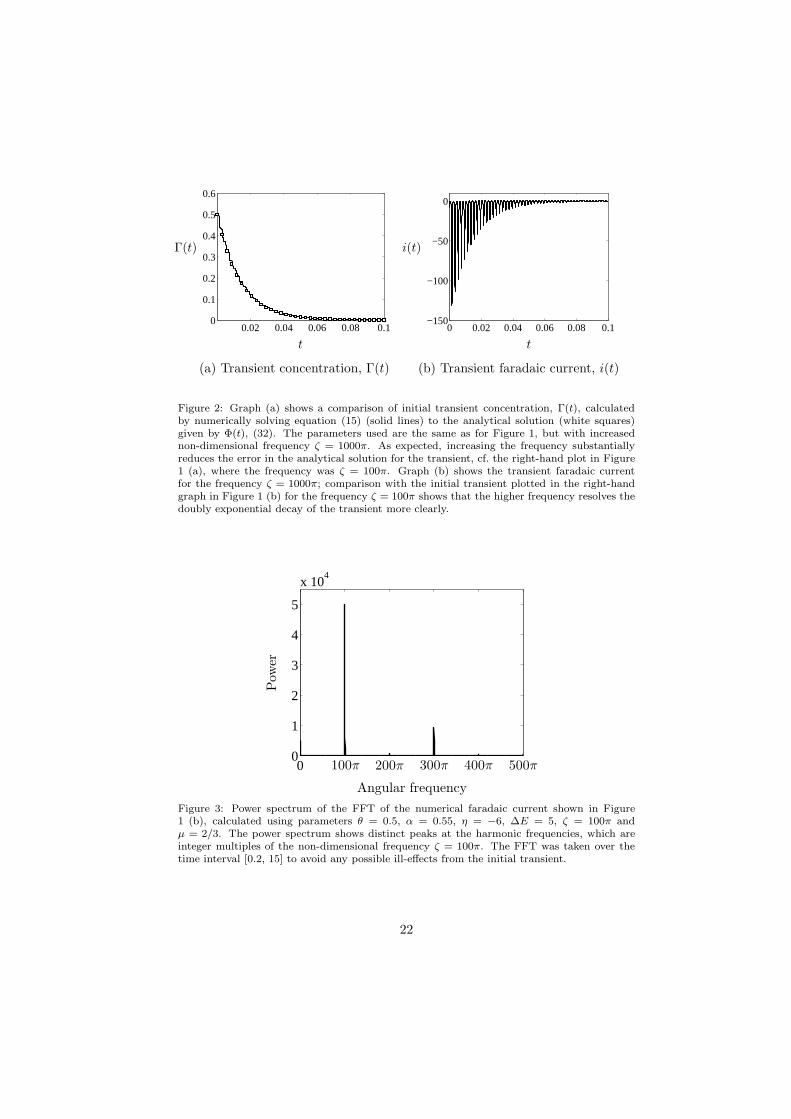
Figure 2: Graph (a) shows a comparison of initial transient concentration, Γ(t), calculatedby numerically solving equation (15) (solid lines) to the analytical solution (white squares)given by Φ(t), (32). The parameters used are the same as for Figure 1, but with increasednon-dimensional frequency ζ = 1000π. As expected, increasing the frequency substantiallyreduces the error in the analytical solution for the transient, cf. the right-hand plot in Figure1 (a), where the frequency was ζ = 100π. Graph (b) shows the transient faradaic currentfor the frequency ζ = 1000π; comparison with the initial transient plotted in the right-handgraph in Figure 1 (b) for the frequency ζ = 100π shows that the higher frequency resolves thedoubly exponential decay of the transient more clearly.
00
1
2
3
4
5
x 104
Angular frequency
Pow
er
100π 200π 300π 400π 500π
Figure 3: Power spectrum of the FFT of the numerical faradaic current shown in Figure1 (b), calculated using parameters θ = 0.5, α = 0.55, η = −6, ∆E = 5, ζ = 100π andµ = 2/3. The power spectrum shows distinct peaks at the harmonic frequencies, which areinteger multiples of the non-dimensional frequency ζ = 100π. The FFT was taken over thetime interval [0.2, 15] to avoid any possible ill-effects from the initial transient.
22
0 2 4 6 8 10 12 14−4
−2
0
2
4
t
A1
(a) Fundamental harmonic
0 2 4 6 8 10 12 14−0.1
−0.05
0
0.05
0.1
t
A2
(b) Second harmonic
0 2 4 6 8 10 12 14−0.8
−0.4
0
0.4
0.8
t
A3
(c) Third harmonic
0 2 4 6 8 10 12 14−0.04
−0.02
0
0.02
0.04
t
A4
(d) Fourth harmonic
Figure 4: Envelopes of the first four harmonics of the numerical faradaic current plotted inFigure 1 (b). The solid lines represent the envelopes of the harmonic extracted from the FFTpower spectrum displayed in Figure 3. The white and black squares represent the analyticalestimates given by A
+m, o(t) and A
−m, o(t) respectively, the expression for which is given in
(44). Note that the second and fourth harmonics have a much smaller magnitude than thefirst and third.
23
0 0.02 0.04 0.06 0.08 0.1−25
−20
−15
−10
−5
0
5
t1
Ito
t(t
1,5)
Figure 5: Comparison of the integral of the initial transient numerical current, Itot(t1, 5)(solid line), calculated from (49), to the approximate analytical solution Idc(t1, 5)+C (whitesquares), where Idc(t1, 5) is calculated from (51). The integrals were calculated using Simp-son’s rule with the domain of integration equal to [t1, t1 + 2pπ/ζ] for p = 5 and t1 ∈ (0, 0.1].The parameters used to calculate the numerical faradaic current are the same as for Figure1, but with increased non-dimensional frequency ζ = 1000π, for which the initial transientcurrent is plotted in Figure 2 (b). The current due to double-layer capacitance was added tothe numerical faradaic current using expression (47) with C = 5.
24
10 20 30 40 50 60 70 800%
2%
4%
6%
8%
10%
12%
14%
16%
Sampling points per cycle
Percentageerror
(a) Error in estimate for µ
10 20 30 40 50 60 70 800.0%
0.5%
1.0%
1.5%
2.0%
2.5%
3.0%
3.5%
Sampling points per cycle
Percentageerror
(b) Error in estimate for α
10 20 30 40 50 60 70 800.0%
0.2%
0.4%
0.6%
0.8%
1.0%
1.2%
Sampling points per cycle
Percentageerror
(c) Error in estimate for η
Figure 6: Percentage error in the estimates for µ = 2/3, α = 0.55 and η = −6 as a functionof the sampling frequency of the numerical current response plotted in Figure 1 (b). Theestimates were obtained by fitting the function A±
3, o(t), (44), to the envelopes of the third
harmonic extracted using the FFT as described in Sections 3.1 and 3.3. The errors in theestimates for µ are larger than those for α and η. This analysis indicates that a samplingfrequency greater than 50 points per cycle of the input voltage should ensure that the errorsdue to sampling for all parameters are less than 1%.
25