Embed Size (px)
Citation preview

Republic of Iraq
Ministry of Higher Education and Scientific Research
Thi-Qar University
College of Science
Physics Department
Theoretical Study of Polarization Evolution and
Modal Coupling in Twisted Single Mode Fibers
A Thesis
Submitted to the Council of The College of Science, Thi-Qar
University in Partial Fulfillment of the Requirement of
Master Degree in Physics
By
Noor Ali Nasir B.Sc. 2013
Supervisor
Prof. Dr. Hassan Abid Yasser
2015 A. D 1437 A. H
CHكج

i
الرمحن الرحيم بسم ا
الذي له ما يف السماوات احلمد
اآلخرة يف احلمد وله األرض يف وما
١اخلبرياحلكيموهو
صدق ا العلي العظيم
)١اآلية(سبأسورة

ii
Supervisor Certification
We certify that the preparation of this thesis entitled '' Theoretical Study of
Polarization Evolution and Modal Coupling in Spun Single Mode Fibers ''
was prepared by (Noor Ali Nasir) under our supervision in the department of
physics, College of Science University of Thi-Qar, as a partial fulfillment of the
requirements of the degree of Master of Science in Physics.
Signature :
Name : Dr. Hassan A. Yasser
Title : Professor
Address : Dept. of Physics, College of Science, Thi-Qar University.
Date : / /2015
(Supervisor)
In view of the available recommendation, we forward this thesis for debate by the
Examining Committee.
Signature :
Name : Dr. Emad A. Salman
Title : Assistant Professor
Address : Head of The Dept. of Physics, College of Science, Thi-Qar University.
Date : / /2015

iii
Examining Committee Certificate
We, the examining committee who certify that this thesis entitled '' Theoretical
Study of Polarization Evolution and Modal Coupling in Spun Single Mode
Fibers '' and examining the student (Noor Ali Nasir) in its content and that, in
our opinion, it meet the standards of a thesis for degree of Master of Science in
Physics with excellent degree.
Signature :
Name : Dr. Ahmed F. Atwan
Title : Professor
Address : College of Education/
Mustansiriyah University.
Date : / /2015
(Chairman)
Signature :
Name : Dr. Abul-Kareem M. Salih
Title : Assistant Professor
Address : College of Science/ Thi-
Qar University.
Date : / /2015
(Member)
Signature :
Name : Dr. Haider K. Muhammed
Title : Assistant Professor
Address : College of Education/ Thi-
Qar University.
Date : / /2015
(Member)
Signature :
Name : Dr. Hassan A. Yasser
Title : Professor
Address : College of Science/ Thi-
Qar University.
Date : / /2015
(Supervisor)
Approved by the Council of the College of Science/ Thi-Qar University
Signature :
Name : Dr. Mohammed A. Auda
Title : Professor
Address : Dean of the College of Science/ Thi-Qar University
Date : / /2015

iv
Dedication
To the lord of the worlds
and to my family for their love and support
Noor 2015

v
Acknowledgment
Thanks to Allah the Majesty for everything, and peace upon
Mohammed and his progeny.
I am profoundly grateful to my supervisor Prof. Hassan Abid
Yasser whose combination of deep insight, unfailing support,
encouragement and patience has been greatly inspiring to me.
I would like to thank all the physics department members who
stand behind the master program in this college, and who support the
students in their study and research.
Special thanks to my family, for their support and patience.
Noor 2015

vi
List of Acronyms
CW Continuous waves
DGD Differential group delay
FMM Fixed modulus model
FWM Four wave mixing
GVD Group velocity dispersion
LP Linear polarization
MCVD Modified chemical vapor deposition
OVD Outside vapor deposition
PCD Polarization-dependent chromatic dispersion
PCVD Plasma chemical vapor deposition
PMD Polarization mode dispersion
PMDRF PMD reduction factor
PSP Principle state of polarization
RMM Random modulus model
RMS Root mean square
SBS Stimulated Brillouin scattering
SOP State of polarization
SPM Self phase modulation
SRS Stimulated Raman scattering
TE Transverse electric mode
TM Transverse-magnetic mode
VAD Vapor axial deposition
XPM Cross phase modulation

vii
List of Symbols
Symbol Definition
effA The effective core area
iA Strength of ith resonance
)(zAn The amplitudes and phases of the two modes
a The radius of fiber core
RC Constant rayleigh scattering
c Speed of light in vacuum
D The diffusion constant
MD Modal dispersion
pD The PMD parameter
d Core diameter
12d The walk-off parameter
E
Electric field
),( yxen The electric field distribution
g Photo-elastic coefficients
Bg The Brillouin gain
Rg The Raman gain
mH Axial magnetic field intensity
)(tI The optical intensity
PI Intensity of the pump field
J Jones vectors
L Fiber length
BL Beat length
effL The effective length
WL The walk-off length
cl The correlation length

viii
M Jones matrix
N Number of modes
NA Numerical aperture
samplesN The number of statistically independent samples
2N The nonlinear-index coefficient
n The mean refractive index of core and cladding
exn The effective indices of the 01LP modes polarized in the x-axis
eyn The effective indices of the 01LP modes polarized in the y-axis
gn Group refractive index
)(rn The refractive index profile
1n The refractive index for core
2n The refractive index for cladding
P The total polarization
)( pmdp The probability density function of the DGD
0P The input power
TP The transmitted power
thP The optical power threshold
p The unit vector in the direction of the slower PSP
)(p Combined probability density
q The graded order
R Muller matrix
r The radial distance from fiber axis
s| Jones vector is denoted as ket vector
0T Pulses of width
t| Output Jones vector
V Normalized frequency
g Group velocity

ix
HV The verdet constant
Attenuation constant
R Rayleigh scattering coefficient
)( Propagation constant
c Geometric birefringence
R , L The right and left propagation constants
t The mechanical twist of the fiber core imparts
)(z The twist rate
0 The fiber nonlinearity coefficient
The splitting ratios
The relative refractive index difference
C Total circular birefringence
L Total linear birefringence
n Refractive index difference between the slow and the fast axis
T The time delay
Fiber birefringence
C Fiber circular birefringence
L Fiber linear birefringence
The dielectric tensor describing the anisotropy of the medium
Differential group delay
Total angle of rotation
Pulse spectral width
PSP The bandwidth PSP
0 The initial phase
The relative dielectric constant of the unperturbed fiber
o The vacuum permittivity
, The principal optical axes

x
The ellipticity angle
The wavelength of the light
o The vacuum permeability
44 Elastooptic strain tensor
Differential core stress
2T Averaging over random perturbation
The "first-order" PMD vector
0 The group delay for all polarizations
pmd The DGD between the fast and slow components
The "second-order" PMD vector (frequency derivative)
The "third-order" PMD vector (second frequency derivative)
NL Nonlinear phase shift
3 The fourth-rank tensor
j
The j th-order susceptibility
The azimuth angle
Angular frequency
0 The carrier frequency of the pulse

xi
Table of Contents
Section Address Pages
Dedication iv
Acknowledgments v
List of acronyms vi
List of symbols vii
Table of contents xi
Abstract xiv
CHAPTER ONE
General Introduction
1.1 Optical communication systems 1
1.2 Birefringence in optical fibers 3
1.3 Literature survey 5
1.4 Goal of thesis 12
1.5 Organization of thesis 12
CHAPTER TWO
Characteristics of Optical Fibers
2.1 Introduction 13
2.2 Types of fiber 14
2.2.1 Multimode step index fiber 14
2.2.2 Multimode graded index fiber 15
2.2.3 Single-mode step index fiber 16
2.3 Materials and manufacture 16
2.4 Fiber modes 17
2.5 Losses 19
2.6 Dispersion 22
2.6.1 Chromatic dispersion 22
2.6.1.1 Material dispersion 24
2.6.1.2 Waveguide dispersion 25

xii
2.6.2 Modal dispersion 25
2.6.3 Polarization mode dispersion 26
2.7 Origin of nonlinearity 28
2.8 Nonlinear refraction 29
2.9 Self-phase modulation 30
2.10 Cross-phase modulation 30
2.11 Four-wave mixing 31
2.12 Stimulated inelastic scattering 31
2.13 Mode coupling 32
2.14 Origin of birefringence 33
2.14.1 Core ellipticity 34
2.14.2 Lateral stress 35
2.14.3 Bending 35
2.14.4 Twists 36
2.14.5 Magnetic field 36
2.14.6 Metal layer near the fiber core 36
2.15 Types of birefringence 37
2.15.1 Linear birefringence 38
2.15.2 Circular birefringence 38
2.15.3 Elliptical birefringence 38
CHAPTER THREE
Theoretical Treatments of Birefringence and Polarization Mode Dispersion
3.1 Introduction 39
3.2 Representations of polarization 40
3.2.1 Jones vectors 40
3.2.2 Jones matrices 41
3.2.3 Stokes vectors 42
3.2.4 Poincare sphere 43
3.2.5 Birefringence and polarization mode dispersion vectors 44

xiii
3.3 Bandwidth of the principal states 46
3.4 Impulse response function of PMD 48
3.5 Mode coupling theory 49
3.6 Jones matrices of birefringent fibers 53
3.7 Generalized Jones matrices of birefringent fibers 55
3.8 Averaging process 59
3.9 Extraction of polarization mode dispersion vector 60
3.10 Polarization mode dispersion reduction factor 63
CHAPTER FOUR
Results and Discussion
4.1 Introduction 65
4.2 Conventional distributions 66
4.3 Mode coupling 68
4.4 PMD reduction factor 68
4.5 Minimization of DGD 71
4.6 Polarization rotation in Stokes space 76
4.7 Effect of twist 77
CHAPTER FIVE
Conclusions and Future Works
5.1 Conclusions 83
5.2 Future works 84
APPENDICES
Appendix A:The statistical distribution of PMD 85
Appendix B: Power splitting ratios 87
References 89

xiv
Abstract
The phenomenon of polarization mode dispersion (PMD) emerged as an
effective influential on the properties of the pulses propagating in the optical fiber
after increasing transmission rates to the limits exceeded several terabytes/sec
because the amount of broadening experienced by the pulse become large in
comparison with the width of the original pulse, and this means adding unwanted
errors to transmission system. The basis of the phenomenon of PMD is a
birefringence of orthogonal axes. The birefringence often is considered linearly
and consequently the system will be analyzed mathematically to determine
properties of the resulting pulses. The addition of the issue of twisting to the
optical fiber, the birefringence become nonlinear. Accordingly, the: mode
coupling, polarization component and pulse broadening rate will be changed.
In this work, the twisting effect has been added to the birefringence vector.
In turn, mathematical forms of the mode coupling, polarization components, and
pulse broadening rate were derived. These forms devolves to the well known
mathematical form after neglecting the impact of twisting. Results proved that
the mode coupling has been much affected by each of: the length of the fiber,
state of polarization, the amount of linear birefringence, and twisting rate.
Periodic behavior of the exchange of the power on axes determines by the
selection of a particular values to those effects. On the other hand, the polarization
components in the Stokes space proved occurrence of rotation of state of
polarization as much depends on the same previous factors. Pulse broadening due
to the existence of mentioned effects can be reduced to as little amount as possible
and perhaps to zero depending on the balance between linear birefringence effects
and circular birefringence, where this balance does not depend on length of the
fiber or wavelength when it comes to achieving the lowest broadening possible of
the pulse. As long as seek in the presence of twisting to cancel broadening of
pulse output, the statistical distribution of amount of the broadening will not be
the same as the traditional distributions.

CHAPTER ONEGeneral Introduction

1
CHAPTER ONE
General Introduction
1.1 Optical Communication Systems
The development of the fibers and devices for optical communications began
in the early 1960s and continued strongly today. But the real change came in the
1980s. During this decade the optical communication in the public communication
networks developed from the status of a curiosity into being the dominant
technology [1].
A communication system transmits information from one place to another,
whether separated by a few kilometers or by transoceanic distances, information is
often carried by an electromagnetic carrier wave. Optical communication systems
use high carrier frequencies (~100 THz) in the visible or near-infrared region of the
electromagnetic spectrum. Optical communication systems differ in principle from
microwave systems only in the frequency range of the carrier wave used to carry
the information. It consists of a transmitter, a transmission medium, and a receiver
[2]. The three elements common to all communication systems are shown in
Fig.(1.1).
Optical communication systems can be classified into two broad categories:
guided and unguided. In case of guided lightwave systems, the optical beam
emitted by the transmitter remains spatially confined. Since all guided optical
communication systems currently use optical fibers, the commonly used term for
them is fiber-optic communication systems. In case of unguided optical
communication systems, the beam emitted by transmitter spreads in space,
unguided optical systems are less suitable for broadcasting applications than
microwave systems because beams spread mainly in forward direction [3].

2
Fig.(1.1): Fundamental elements of a communication system [4].
In electrical communications the information source provides an electrical
signal, usually derived from a message signal which is not electrical, to a
transmitter comprising electrical and electronic components which converts the
signal into a suitable form for propagation over the transmission medium, see
Fig.(1.2). The role of optical transmitters is convert an electrical signal into an
optical form and to launch the resulting optical signal into the optical fiber acting as
a communication channel. The role of a communication channel is to transport the
optical signal from transmitter to receiver with as little loss in quality as possible.
An optical receiver converts the optical signal received at the output end of the
fiber link back into the original electrical signal [2,5].
Fig.(1.2): The optical fiber communication system [2].

3
1.2 Birefringence in Optical Fibers
Birefringence is a term used to describe a phenomenon that occurs in
certain types of materials, in which light is split into two different paths. This
phenomenon occurs because these materials have different indices of refraction
depending on the polarization direction of light, this is also observed in an optical
fiber due to the slight asymmetry in the fiber core cross-section along the length
and external stresses applied on the fiber such as bending. In ideal isotropic fiber no
birefringence it propagates any state of polarization (SOP) launched into the fiber
unchanged. While real fibers possess some amount of anisotropy owing to an
accidental loss of circular symmetry, this loss is due to a noncircular geometry of
the fiber [6].
In a birefringence fiber, the effective mode index varies continuously with
the field orientation angle in the transverse plane. The directions that correspond to
the maximum and minimum mode indices are orthogonal and define the principal
axes of the fiber. Let us assume that these principal axes coincide with the x-axis
and y-axis. The fiber birefringence is given by )/( effyx nc , where x
and y are the propagation constants according to x and y axes, yxeff nnn .
Typically, effn range between 10-7 and 10-5, which is much smaller than the index
difference between core and cladding (~3×10⁻³), xn and yn are the effective mode
indices associated with x and y polarizations, respectively, is the angular
frequency, and c is the speed of light in vacuum. The difference can also change
the SOP of the light as it travels along the fiber [7].
Polarization mode dispersion (PMD) is caused by the birefringence of optical
fiber and the random variation of its orientation along the fiber length. PMD causes
different delays for different polarizations, and when the difference in the delays
approaches a significant fraction of the bit period, pulse distortion and system

4
penalties occur. Environmental changes including temperature and stress cause the
fiber PMD to vary randomly in time, making PMD particularly difficult to manage
or compensate. There are two origins of birefringence in optical fiber are variations
of the fiber from in ideal cylindrical geometry, and the presence of residual
mechanical stress or strain in the fiber core [8]. The birefringence can be also
described in terms of the beat length which is defined as /2BL , where BL is
the beat length. The physical meaning of the beat length is that the SOP of light is
reproduced after traveling a distance of BL as shown in Fig. (1.3) [9,10].
Fig.(1.3): Evolution of SOP along a polarization-maintaining fiber when input
signal is linearly polarized at 45 from the slow axis [10].
Twisting of birefringence fibers produces two effects simultaneously. First,
the principal axes are no longer fixed but rotate in a periodic manner along the fiber
length. Second, shear strain induces circular birefringence in proportion to the twist
rate for the fiber [10,11]. A twist rate of around five turns per meter is sufficient to
reduce crosstalk significantly between the polarization modes. The reduction
occurs because a high degree of circular birefringence is created by the twisting
process [2].

5
1.3 Literature Survey
In 1970, L. Cohen et al., [12] described experiments on crab leg nerves and
squid axons in which the magnitude of the retardation change during the conducted
action potential was determined, and in which its localization and the orientation of
its optic axis were established.
In 1972, D. Gloge [13] shown that the parabolic grading of the core index in
a multimode fiber affects the mode volume and the loss in bends very little, if the
index difference of the graded core is twice as much as the homogeneous core.
Mode coupling in random bends is slightly decreased by grading, both the graded
and the homogeneous multimode fiber are particularly sensitive to certain critical
deviations of the guide axis from straightness.
In 1973, W. Gambling and H. Matsumura [14] studied an analysis that has
been made of pulse dispersion in an optical fiber having a continuous radial
variation of refractive index. Solutions are presented for Selfoc fiber showing the
effects of mode and material dispersion and group delay, where the predicated
dispersions range from very low values up to about 1ns/km, depending on the
launching conditions.
In 1975, D. Marcuse and H. Presby [15] determined the variations in the
geometry of a step-index optical fiber as functions of position along the axis by an
analysis of the backscattered light produced when a beam of a laser is incident
perpendicular to the optical fiber axis. The theoretical calculations support
experimental observations and account for a partial reduction in the multimode
pulse dispersion.
In 1976, D. Marcuse [16] presented formulas for the microbending losses of
fibers that are caused by random deflections of the fiber axis. Loss formulas for the
single-mode fiber are derived from coupled-mode theory using radiation modes.

6
In 1979, M. Adams et al., [17] studied the birefringence in optical fibers with
elliptical cross-section, where a comparison is made between various
approximations for the phase delay between orthogonally polarized modes in
elliptical optical fibers. A lower value for the birefringence produced by a given
ellipticity, the effect on fiber bandwidth is shown to be small compared to that
resulting from stress birefringence.
In 1980, H. Sunak and J. Neto [18] discussed pulse dispersion in optical
fibers and outline the various mechanisms which contribute to it. The magnitude of
each dispersion mechanism in different types of fibers is outlined and its effect on
the: information carrying capacity discussed. A nanosecond test facility, for
intermodal dispersion measurements are discussed in detail, together with the
procedure of its operation.
In 1981, A. Barlow et al., [19] presented a theoretical and experimental
analysis of the polarization properties of twisted single-mode fibers. It showed that
whereas a conventionally twisted fiber possesses considerable optical rotation, a
fiber which has a permanent twist imparted by spinning the preform during fiber
drawing exhibits almost no polarization anisotropy.
In 1981, J. Sakai and T. Kimura [20] showed that birefringence and the PMD
caused by: elliptical core, twist, pure bending, transverse pressure, and axial tension
are studied by treating these deformations as perturbations to step-index single-
mode fiber with a round core. These effects are formulated in terms of fiber
structure and perturbations parameters and are compared comprehensively.
In 1982, D. Payne et al., [21] illustrated that the polarization of single-mode
optical fibers are easily modified by environmental factors. While this can be
exploited in a number of fiber sensor devices. It can be troublesome in applications
where a stable output polarization-state is required. Low-birefringence fibers are
described which are made by spinning the preform during the draw.

7
In 1983, I. White and S. Mettler [22] presented an electromagnetic modal
theory for characterizing parabolic-index multimode fiber splices with either
intrinsic or extrinsic mismatches. The theory agrees with previously published
theoretical results for transverse offset using a uniform power distribution.
In 1987, C. Tsao [23] explained the formulas determining the polarization
ellipse from a given electric fields components and vice versa. The objective of this
paper has been then to study the polarization evolution in a curvilinear optical fiber
with both linear and circular birefringence. As a result the Jones matrix-coupled
mode description has been extended to cover a fiber with distributed principle axis
and linear and circular birefringence.
In 1988, C. Shi and R. Hui [24] presented a theoretical analysis on the mode-
coupling effect in single-mode, single polarization optical fibers. When an optical
fiber undergoes external perturbations, polarization coupling is induced, and there
is continuous exchange of energy between the guided and leaky modes. The leaky
mode also leaks some energy to the cladding; therefore, the energy carried by the
guided mode dissipates through polarization mode coupling.
In 1989, S. Poole et al., [25] showed that the techniques for the measurement
of the diverse properties of all these different optical fibers are presented with
results and, where appropriate, the problems with their characterization are
discussed.
In 1991, N. Gisin et al., [26] measured PMD in short and long single-mode
fibers by a polarization maintaining Michelson interferometer. Found a
nonnegligible PMD in some standard fibers, the sensitivity enables us to measure
the bend induced PMD of a fiber rolled on a 26-cm diameter drum. A theoretical
model for PMD with random mode coupling is developed and an explicit equation
for the time of flight distribution is presented.

8
In 1993, C. Poole and T. Darcie [27] described that the analog transmission
in single-mode fiber using chirped sources gives rise to nonlinear distortion when
polarization-mode dispersion is present. Then investigated experimentally and
theoretically two mechanisms for this distortion: for chirped sources, PMD in the
presence of polarization-mode coupling results in second-order distortion that is
proportional to the square of the modulation frequency.
In 1996, P. Wai and C. Menyuk [28] calculated PMD and the polarization
decorrelation and diffusion lengths in fibers with randomly varying birefringence.
Two different physical models in which the birefringence orientation varies
arbitrarily have been studied and shown to yield nearly identical results.
In 2000, A. Galtarossa et al., [29] the statistical properties of the random
birefringence that affects long single-mode fibers have been experimentally
evaluated by means of a polarization-sensitive optical time-domain reflectometry.
The measurements have been in good agreement with theoretical predictions and
show, for what we believe is the first time, that the components of the local
birefringence vector are Gaussian random variables.
In 2001, I. Lima et al., [30] analyzed PMD emulators comprised of a small
number of sections of polarization-maintaining fibers with polarization scattering at
the beginning of each section. They derived analytical expressions and determined
two main criteria that characterize the quality of PMD emulation. The experimental
results are in good agreement with the theoretical predictions.
In 2002, Y. Tan et al., [31] determined the transient evolution of the
probability distribution of the polarization dispersion vector both analytically and
numerically, using a physically reasonable model of the fiber birefringence. They
showed that the distribution of the differential group delay (DGD), which is the
magnitude of PMD vector, becomes Maxwellian distribution and takes much
longer, of the order of tens of kilometers.

9
In 2003, A. Galtarossa et al., [32] derived an analytical formula for the mean
DGD of a periodically spun fiber with random birefringence. They modeled the
birefringence with fixed modulus and a random orientation under the condition that
the spin period is shorter than the beat length. They numerically compared the
analytical results with those given by the random-modulus model of birefringence,
and they obtained good agreement.
In 2004, D. Nolan et al., [33] discussed recent progress in the understanding
of the fabrication and characteristics of the fibers, also discussed the important fiber
physical parameters, including the fiber index profile and the fiber spinning
parameters and their impacts on the realization of the low PMD performance.
Also in 2004, L. Yan et al., [34] demonstrated a practical PMD emulator
used programmable DGD elements. The output PMD statistics of the emulator can
be chosen by varying the average of the Maxwellian DGD distribution applied to
each element. This technique is used to measure the Q-factor degradation due to
both average and rare PMD values in a 10-Gb/s transmission system.
In 2005, X. Chen et al., [35] reviewed and reported the progress in
understanding the properties of polarization evolution in spun fibers in both of the
cases with and without the influence of external factors. Theoretical formalism is
constructed and various properties of the polarization evolution are revealed
through numerical modeling.
In 2006, H. Yasser [36] showed that the reconstructed pulse width in present
of PMD and chromatic dispersion may be controlled using the properties of fiber
and the propagated pulses.
In 2006, L. Yan et al., [37] showed that the PMD still remains a challenge
for high-data-rate optical-communication systems. Practical solutions are desirable
for PMD emulation, monitoring, and compensation.

10
In 2007, J. Lee [38] analyzed the PMD vector distribution for linear
birefringent optical fibers. Assumed the linear birefringence vector components as
white Gaussian processes, find an asymptotic solution for the probability density
function of the PMD vector, the analysis shown that the PMD vector distribution is
dependent on the polar angle during its transient and the distribution tail for the
magnitude of the PMD vector is higher than the Maxwellian.
In 2008, Z. Li et al., [39] proposed a theoretical approach to analyze the
pressure stress distribution in single mode fibers and achieve the analytical
expression of stress function, from which they obtained the stress components with
their patterns in the core and computed their induced birefringence. They used
Mueller matrix method to measure the birefringence vectors which are employed
to compute the pressure magnitudes and their orientation.
In 2009, T. Xu et al., [40] developed a method to measure the spatial
distribution of polarization mode coupling with random modes excited using a
white light Michelson interferometer. The influence of incident polarization
extinction ratio on polarization coupling detection has been evaluated theoretically
and experimentally.
Also in 2009, H. Wen et al., [41] used two methods to measure the linear
birefringence and circular birefringence of a commercial photonic band gap fiber
around 1.5 µm. The linear birefringence beat length is found to vary significantly
with wavelength, while the circular birefringence is observed to be weaker by a
factor of at least ten.
In 2010, H. Yasser [42] presented an accurate mathematical analysis to
increase the rates of transmission, which contain all physical variables contribute to
determine the transmission rates. New mathematical expressions for: pulse power,
peak power, time jittering, pulse width, and power penalty are derived. On the basis
of these formulas, choose a certain operating values to reduce the effects of PMD.

11
In 2011, A. Mafi et al., [43] presented a method for ultra-low-loss coupling
between two single mode fibers with different mode field diameters using
multimode interference in a graded-index multimode optical fiber. They performed
a detailed analysis of the interference effects and showed that the graded-index
fiber can also be used as a beam expander or condenser.
In 2012, I. Khan [44] described an analytical approach of Jones matrix
method to analyze for optical system design. Before commercial production of any
optical system it is necessary to check the compatibility and final output checking
of system. This checking can be done very easily by using Jones matrix method.
In 2013, H. Yasser and N. Shnan [45] proved that the presence of PMD
vector leads to DGD among the polarization components, while the presence of
polarization dependent loss vector leads to attenuating one of components and
increases the other by a magnitude determine by polarization dependent loss value.
In 2013, D. Tentori and A. Weidner [46] analyzed the birefringence matrix
developed for a twisted fiber in order to identify the basic optical effects that define
its birefringence, using differential Jones calculus. The resultant differential matrix
showed three independent types of birefringence: circular, linear at 0 degrees and
linear at 45 degrees.
In 2014, G. Prakash pal and M. Gupta [47] showed that the signal
degradation in optical fiber due to dispersion, intermodal distortion or modal delay
appears only in multimode fibers but intramodal dispersion occurs in all types of
optical fiber and results from the finite spectral line width of the optical source.
In 2015, M. Yamanari et al., [48] demonstrated a prototype system of
polarization-sensitive optical coherence tomography designed for clinical studies of
the anterior eye segment imaging. The system can measure Jones matrices of the
sample with depth-multiplexing of two orthogonal incident polarization and
polarization-sensitive detection.

12
1.4 Aim of Thesis
The present work aims at: 1) studying the origin of fiber birefringence and
fiber twist, 2) analyzing the mode coupling that may be happen in presence of
PMD, 3) explaining the Jones matrices for the concatenated segments that form the
entire fiber, where for each segment the matrix must simulate the real variations, 4)
mixing the effects of linear and circular birefringence and construct a unified
description of the output PMD vector, 5) minimizing the resulted DGD under the
above effects, and 6) studying the polarization rotation in Poincare sphere.
1.5 Organization of Thesis
The work of this study falls into five chapters. After the introducing chapter
(chapter one), chapter two presents the basic properties of fiber optics.
Furthermore, the representation of the origin of fiber birefringence is illustrated
using different orientations that are present in the literatures review. Chapter three
presents the theoretical managements of mode coupling, polarization rotation, fiber
twist and the reconstructed PMD vector. Moreover, the subject is obtained in the
view of Poincare sphere. Chapter four contains the results and discussions. Finally,
chapter five summarizes the conclusions and the suggested future works.

CHAPTER TWOCharacteristics of Optical Fibers

13
CHAPTER TWO
Characteristics of Optical Fibers
2.1 Introduction
Optical fiber is the medium in which communication signals are
transmitted from location to another in the form of light guided through thin fibers
of glass or plastic. These signals are digital pulses or continuously modulated
analog streams of light representing information. These same types of information
can be sent on metallic wires such as twisted pair and coax and through the air on
microwave frequencies. The reason to use optical fiber is that it offers advantages
not available in any metallic conductor or microwave [49].
Fiber-optic communication systems possess some advantages as: law
transmission loss, large capacity of information transmission and no
electromagnetic interference, lighter weight than copper, no sparks even when
short-circuited, higher melting point than copper, and practically inexhaustible
raw material supply [50].
An optical fiber is composed of a very thin glass rod, which is surrounded
by a plastic protective coating. The glass rod contains two parts: the inner portion
of the rod called (core) and the surrounding layer called (cladding). Light injected
into the core of the glass fiber follows the physical path of the fiber due to the
total internal reflection of the light between the core and the cladding, the fiber
type is closely related to the diameter of the core and the cladding and how the
light travels through it as shown in Fig.(2.1). The core and the cladding have
different refractive indices, the fiber core has a higher index of refraction than the
refractive index of surrounding cladding. The light will be totally reflected every
time it strikes the core-cladding interface. For typical fibers used in
communication systems, the refractive index difference between core and
cladding is about 0.01-0.03 [51,52].

14
Fig.(2.1): Composition of optical fiber [52].
2.2 Types of Fiber
There are three basic types of fiber optic cable as in Fig.(2.2), which are
used in communication systems. In the following subsections, the basic
characteristics of these types will be summarized.
Fig.(2.2): Types of optical fibers [49].
2.2.1 Multimode Step Index Fiber
It is the simplest type of fiber and has a core diameter in the 50 m to more
than 1000 m range. The large core of this fiber allows many light modes to
propagate, where the light passing down the fiber takes longer and shorter path
lengths, consequently the signal is dispersed in time (modal dispersion). This type

15
of fiber is generally used for short data links and control circuits but not usually
for telecommunications. The refractive index profile is defined as [53]
(2.1) 2
1
claddingarn
corearnrn
where 1n is the refractive index for core, 2n is the refractive index for cladding, a
is the radius of fiber core and r is the radial distance from fiber axis.
2.2.2 Multimode Graded Index Fiber
A graded index fiber core actually consists of many concentric glass layers
with refractive indices that decrease with the distance from the center, the modal
dispersion in graded index fiber can be reduced to as little as 1ns/km. The index
variation may be represented as [54]
(2.2) 21
/21
21
1
claddingarnn
coreararnrn
q
where is the relative refractive index difference and q is the profile parameter
which gives the characteristic refractive index profile of the fiber core,
representation of step index profile when q , parabolic profile when 2q ,
triangular profile 1q as shown in Fig.(2.3) [55]. The graded index profiles which
at present produce the best results for multimode optical propagation have a near
parabolic refractive index profile core with 2q . Graded index fibers are
therefore sometimes referred to as inhomogeneous core fibers [2].
Fig.(2.3): Possible fiber refractive index profiles for differentq [55].

16
2.2.3 Single-Mode Step Index Fiber
Single mode step index fiber limits the amount of dispersion by having a
core small enough to allow only one mode of light to travel through the fiber
(about 10µm). This fiber has extremely high bandwidths and is currently used in
telecommunication and long distance high capacity links [53].
2.3 Materials and Manufacture
The most widely used optical fibers in transmission are "all silica" fibers,
mode with silica, and germanium oxide core "doping" which determines index
value and profile, they turn into multimode fibers especially graded-index and
single mode fibers. By erbium doping, they are also mode into amplifying fibers.
Plastic fibers, besides their lighting applications, progress for very short distance
transmissions. There are other materials for much more specific applications. The
basic material used in the manufacture of optical fiber is vitreous silica dioxide
(SiO2), but to achieve the properties required from a fiber, various dopants are
also used: (Al2O3, B2O3, GeO2, P2O5). Their task is to slightly increase and
decrease the refractive index of pure silica (SiO2). Initially the fiber losses were
high, but through improvements in the quality of the materials and the actual
production process, the losses have been reduced so as to be close to the
theoretical expected losses [50].
Preparation of silica fibers consists of two major processes: perform
making and drawing. The attenuation and the dispersion characteristics of optical
fibers largely depend on the perform making process, while glass geometry
characteristics and strength depend on the drawing process. There are several
methods used today to fabricate moderate-to-low loss waveguide fibers are:
modified chemical vapor deposition (MCVD), plasma chemical vapor deposition
(PCVD), outside vapor deposition (OVD) and vapor axial deposition (VAD). The
method MCVD was developed by Bell Telephone Laboratories and others in
1974 [56]. In this process, successive layers of SiO2 are deposited on the inside
of a fused silica tube by mixing the vapors of SiCl4 and O2 at a temperature of

17
about 1800o C. To ensure uniformity, a multiburner torch is moved back and forth
across the tube length using an automatic translation stage. The refractive index of
the cladding layers is controlled by adding fluorine to the tube. When a sufficient
cladding thickness has been deposited, the core is formed by adding the vapors of
GeCl4 or POCl3, these vapors react with oxygen to form the dopants GeO2 and
P2O5 [3]. The reaction which produces the dopant is
GeCl4 + O2 → GeO2 + 2Cl2
4POCl3 + 3O2 → 2P2O5 +6Cl2 )3.2(
The basic advantage of the MCVD process is that the waveguide structure
and properties can be built into the preform and retained in the finished fiber. The
relative dimensions and the index profile of the preform are transferred to the
finished fiber during the drawing process [52]. Fig.(2.4) illustrates the schematic
representation of MCVD.
Fig.(2.4): Schematic representation of MCVD [1].
2.4 Fiber Modes
The modes are mathematical and physical ways of describing the
propagating of electromagnetic waves in an arbitrary medium. It is a permitted
solution to Maxwell's equation. For the sake of simplicity, a mode can be
described as a possible direction (route ) that the light wave will follow down, a
certain mode will also transport a certain amount of energy. The fiber used today
is either of type that transmits only one mode (called single mode fiber) or of the
type that transmits generally hundreds of modes (called multimode fiber) [52].

18
There are two types of fiber modes designated as mn and mn . For
0m these modes are analogous to the transverse-electric (TE) and transverse-
magnetic (TM) modes of planar waveguide because the axial component of the
electric field, or the magnetic field, vanishes. However for 0m , fiber modes
become hybrid i.e. all six components of the electromagnetic field are non zero
[10]. Fig.(2.5) explains different modes.
Fig.(2.5): The electric field configurations for the three lowest linear polarization
(LP) modes illustrated in terms of their constituent exact modes: a) LP mode
designations, b) exact mode designations, c) electric field distribution of the exact
modes, d) intensity distribution of EX for the exact modes indicating the electric
field intensity profile for the corresponding LP modes [2].

19
The number of modes possible in a fiber depends on the diameter of the
core, the wavelength of the light, and the core's numerical aperture. The numerical
aperture is defined as [54]
(2.4) 22claddingcore nnNA
The fiber parameter or normalized frequency for a single-mode fiber be 4045.2V
while for multi-mode fiber 10V , where the dimensionless parameter V is
defined by the relation [57]
(2.5) 22 NAd
nnd
V claddingcore
where d is core diameter and is the wavelength. Using this definition, the
number of modes of multimode fibers will be [1]
(2.6) 4
22
2
fiberindexgradedV
N
fiberindexstepV
N
Note that, the number of modes increases by increasing of the graded order q that
defined in Eq. (2.2).
2.5 Losses
The attenuation is caused by two physical effects which are absorption and
scattering. The absorption has an effect of removing photons when they interact
with atoms and molecules of the medium, it occurs when the energy of photon is
equal to difference between two electronic energies, while the scattering losses
occur when the photons undergo a variation in the core's refractive index, this
phenomenon is termed Rayleigh scattering and considered as an intrinsic loss in
optical fiber. The lowest attenuation occurs at wavelengths 1300 nm and 1550 nm
with corresponding values of 0.5 dB/km and 0.2 dB/km, respectively. For fiber of
length L , the transmitted power TP is given by [58]
(2.7) exp0 LPPT
where the attenuation coefficient is a measure of total fiber losses from all
sources. It is customary to express in units of dB/km using the relation [59]

The intrinsic loss level is estimated to be in
where the constant RC
constituents of fiber core. As
silica fibers are dominated by Rayleigh sca
occurs when impurities such as water or ions of materials such as copper
chromium absorb certain wave
minimum of attenuation [54
The Rayleigh scattering
occurring on a small scale compared with the wave
subsequent scattering due to th
directions produce an attenuation proportional to
by such inhomogeneities is mainly in the forward direction, de
fiber material, design and manufacture Mie scattering can cause significant losses
[2]. Fig.(2.6) illustrates the wave
mechanisms.
Fig.(2.6): Loss spectrum of a single
20
343.4log10
0
P
P
LT
dB
he intrinsic loss level is estimated to be in (dB/km) as
/ 4 RR C
is in range 9.07.0 dB/(km-µm 4 ) depending on the
constituents of fiber core. As 15.012.0 R dB/km near
silica fibers are dominated by Rayleigh scattering. In an optical fiber, absorption
hen impurities such as water or ions of materials such as copper
chromium absorb certain wavelengths manufactures can produce fibers with a
attenuation [54].
cattering results from inhomogeneities of random nature
ll scale compared with the wavelength of
subsequent scattering due to the density fluctuations, which are
an attenuation proportional to 4/1 . The Mie scattering created
homogeneities is mainly in the forward direction, de
fiber material, design and manufacture Mie scattering can cause significant losses
Fig.(2.6) illustrates the wavelength dependence of several fundamental loss
Loss spectrum of a single-mode fiber produced
(2.8)
(2.9)
) depending on the
55.1 µm, losses in
. In an optical fiber, absorption
hen impurities such as water or ions of materials such as copper or
lengths manufactures can produce fibers with a
homogeneities of random nature
length of the light, the
e density fluctuations, which are in almost all
e scattering created
homogeneities is mainly in the forward direction, depending upon the
fiber material, design and manufacture Mie scattering can cause significant losses
ral fundamental loss
mode fiber produced in 1979 [3].

21
Losses can also occur by microbending in the case of mechanical
constraints in the fiber. Single mode fibers are rather less sensitive to bending
than multimode fibers (but their losses quickly increase with the mode diameter,
therefore with the wavelength). This sensitivity generally decreases when the
core/cladding index difference increases hence the advantage for high numerical
aperture fibers in cabling where a higher risk of strong bending exists (in
buildings for example) [50].
Generally, there are two types of bend that cause losses. The first is referred
to as a macrobending. This is where the cable is installed with a bend in it that has
a radius less than the minimum bending radius, light will strike the core/cladding
interface at an angle less than the critical angle and will be lost into the cladding.
The second type of bending loss is referred to as a microbending, the microbend
takes the form of a very small sharp bend in the cable. Microbends can be caused
by imperfections in the cladding, ripples in the core/cladding interface, ting cracks
in the fiber and external forces. The external forces may be from a heavy sharp
object being laid across the cable or from the cable being pinched, as it is pulled
through a tight conduit. As for the occurrence of macrobends, the light ray will hit
the bend at an angle less than the critical angle and will be refracted into cladding
[4].
Connector insertion loss is not just a function of the tolerance of the
connector but also the tolerance of the fiber itself. There are three losses at
connections: loss by Fresnel reflection during consecutive light crossing of two
air-glass interfaces. This loss is of 8℅ (or 0.35 dB) and the reflected light may
create disruptions. It can be avoided by splicing or by using adapted techniques in
the case of connectors, loss caused by difference between parameters (diameter
and numerical apertures) of two fibers, this difference would come from
manufacturing tolerance on diameters, indices and core-cladding concentricity,
and loss caused by bad relative positioning of two fibers [50,53]. Fig.(2.7)
explains different sources of losses.
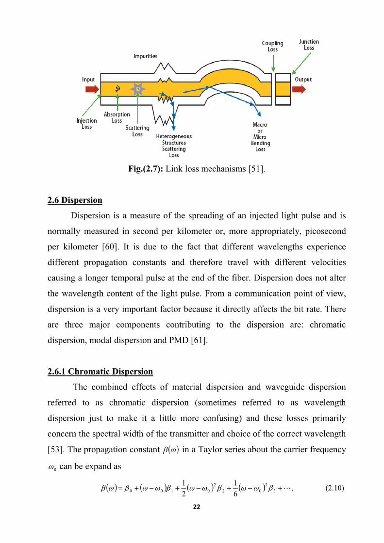
22
Fig.(2.7): Link loss mechanisms [51].
2.6 Dispersion
Dispersion is a measure of the spreading of an injected light pulse and is
normally measured in second per kilometer or, more appropriately, picosecond
per kilometer [60]. It is due to the fact that different wavelengths experience
different propagation constants and therefore travel with different velocities
causing a longer temporal pulse at the end of the fiber. Dispersion does not alter
the wavelength content of the light pulse. From a communication point of view,
dispersion is a very important factor because it directly affects the bit rate. There
are three major components contributing to the dispersion are: chromatic
dispersion, modal dispersion and PMD [61].
2.6.1 Chromatic Dispersion
The combined effects of material dispersion and waveguide dispersion
referred to as chromatic dispersion (sometimes referred to as wavelength
dispersion just to make it a little more confusing) and these losses primarily
concern the spectral width of the transmitter and choice of the correct wavelength
[53]. The propagation constant in a Taylor series about the carrier frequency
0 can be expand as
(2.10) ,6
1
2
13
302
20100

23
where
(2.11) ,2,10
md
dm
m
m
The cubic and higher-order terms in this expansion are generally negligible
if the pulse spectral width 0 . Their neglect is consistent with the quasi-
monochromatic approximation. If 02 for some specific values of 0 (in the
vicinity of the zero-dispersion wavelength of the fiber, for example), it may be
necessary to include the cubic term. The term 2 describing the frequency
dependence of the group velocity is the chromatic dispersion or group velocity
dispersion (GVD) of the fiber. The parameters 1 and 2 are related to the
refractive index n and its derivatives through the relations [62]
(2.12) )(
)(11
0
01
d
dnn
cc
ng
g
(2.13) 21
2
21
2
d
nd
d
dn
cd
d
where gn is group index, g is group velocity, c speed of light in vacuum.
Fig.(2.8) explains the relations between n , gn and the wavelength [55]. The walk-
off parameter 12d defined as [5]
(2.14) 21
11
211112 ggd
where 1 and 2 are the center wavelengths of two pulses. For pulses of width 0T ,
can define the walk-off length WL by the relation
(2.15) / 120 dTLW
In normal-dispersion regime 02 a longer wavelength pulse travels faster,
high-frequency (blue-shifted) components of an optical pulse travel slower than
low-frequency (red-shifted) components of the same pulse. While the opposite
occurs in anomalous-dispersion regime. The group-velocity mismatch plays an
important role for nonlinear effects involving cross modulation [10].

24
Fig.(2.8): n and gn as functions of wavelength for fused silica [55].
2.6.1.1 Material Dispersion
Material dispersion is caused by variations of refractive index of the fiber
material with respect to wavelength. Since the group velocity is a function of the
refractive index, the spectral components of any given signal will travel at
different speeds and cause deformation of the pulse. Variations of refractive index
with respect to wavelength are described by the following Sellmeier equation
[53,10]
(2.16) 122
22
i i
iAn
where iA is the magnitude of the i th resonance, whereas and i are the
wavelengths corresponding to frequencies and i , respectively, the refractive
index decreases with increasing wavelength. This behavior is important to
describe the material origins of GVD. Fig. (2.9) explains the components of
chromatic dispersion [3,7]. When manufacturing single-mode fibers, not only is
the diameter reduced, but also the difference between the core and the cladding
refractive indices is reduced. Here the effect of modal dispersion disappears, but
then material dispersion becomes the significant problem. The effects of material
dispersion become more noticeable in single-mode fibers because of the higher
bandwidth (data rates) that are expected of them [4].

25
Fig.(2.9): Total dispersion and relative contributions of material dispersion and
waveguide dispersion for a conventional single-mode fiber [3].
2.6.1.2 Waveguide Dispersion
Waveguide dispersion occurs in single mode fibers, where a certain amount
of the light travels in cladding, i.e., the dispersion occurs because the light moves
faster in low refractive index cladding than in the higher refractive index core.
The degree of waveguide dispersion depends on the proportion of light that
travels in cladding [4]. Waveguide dispersion depends on the dispersive
properties of the waveguide itself (e.g. the core radius and the index difference), a
significant property is that the waveguide dispersion has opposite signs with
respect to the material dispersion in the wavelength rang above 1300 nm. This
property can be used to develop dispersion shifted fibers choosing suitable values
for the core radius and for the index difference [56].
2.6.2 Modal Dispersion
Modal dispersion typically occurs with multimode fiber, when a very short
light pulse is injected into the fiber within the numerical aperture, all of the
energy does not reach the end of the fiber simultaneously. Different modes of
oscillation carry the energy down the fiber using paths of differing lengths, the
pulse spreading by virtue of different light path lengths is called modal dispersion,

26
or more simply, multimode dispersion. Modal dispersion increases with
increasing the numerical aperture and therefore, the bandwidth of the fiber
decreases with an increase in numerical aperture, the same rule applies to the
increasing diameter of a fiber core. It is given by [51, 61]
(2.17)
8
2
mod
fiberindexgradedforc
n
fiberindexstepforc
n
D
g
g
2.6.3 Polarization Mode Dispersion
PMD is a property of a single mode fiber or an optical component in which
signal energy at a given wavelength is resolved into two orthogonal polarization
modes with different propagation velocities, resulting difference in propagation
time between polarization modes known as differential group delay (DGD) leads
to pulse broadening. The causes of PMD is a phenomenon called birefringence
[62]. In the time-domain picture, for a short section of fiber, the DGD, can be
found from the frequency derivative of the difference in propagation constants
[8]
(2.18)
d
nd
cc
n
d
d
L
This "short-length" or "intrinsic" PMD, L/ , is often expressed in units of
picoseconds per kilometer of fiber length L . PMD is characterized by the root-
mean square (RMS) value of the time delay 1 LT , obtained after averaging
over random perturbation. The variance of T is found to be [10]
(2.19) 1//exp2)( 21
22 cccT lLlLlT
where L/1 is related to group-velocity mismatch, and the correlation
length cl is defined as the length over which two polarization components remain
correlated; typically values of cl are of the order of 10m. For 1.0L km, we can
use Llc to find that [5]

27
)(2.20 L21 pcT DLl
where pD is the PMD parameter. For most fibers, the value of pD is in the range
of (0.01 to 1) ps/ km , because of its L dependence. Due to the random
polarization mode coupling, the propagation of a pulse through a long-length fiber
is extremely complicated, in case of narrow bandwidth input signal even for long
fibers, one can still find two special orthogonal polarization states at the fiber
input that result in an output pulse undistorted to first order. These two orthogonal
states of polarization are called principle states of polarization (PSPs). In the
frequency domain, a PSP is defined as that input polarization for which the
output SOP is independent of frequency to the first order [63]. Fig.(2.10) explains
the basic concept of PMD phenomenon.
Fig.(2.10): Impact of PMD on the propagating pulse [62].
When higher-order PMD effects are considered,
is usually called the
"first-order" PMD vector, its frequency derivative is the "second-order" PMD
vector, the second derivative is the "third-order" PMD vector. The higher-
order PMD effects can be included by expanding the PMD vector in a Taylor
series around the carrier frequency 0 of the pulse as [64]
)(2.21 |2
|)()(00 2
22
0
d
d
d
d
So-called second-order PMD is then described by the derivative [65]

28
(2.22) ˆˆ pp
d
d
The first term on the right-hand side of Eq.(2.22) is
, the component of that
is parallel to
, whereas the second term is the component of
that is
perpendicular to . Fig.(2.11) shows a vector diagram of the principal parameters
and their interrelationship [66]. The magnitude of the first term
is the change
of the DGD with wavelength and causes polarization-dependent chromatic
dispersion (PCD). The second term in Eq.(2.22), p described PSP
depolarization, which represents a rotation of the PSPs with frequency [8].
Fig.(2.11): Schematic diagram of the PMD vector )(
and the second-order
PMD components showing the change of )(
with frequency [66].
2.7 Origin of Nonlinearity
In addition to the linear response, an electric field produces a polarization
that is a nonlinear function of the field. The nonlinear response can give rise to an
exchange of energy between a number of electromagnetic fields of different
frequencies. The total polarization P
induced by electric dipoles is not linear in
the electric field E
, but satisfied the more general relation [67]

29
(2.23) , 321
0 EEEEEErP
where 0 is vacuum permittivity and
,2,1jj is the j th-order susceptibility.
However, nonlinear effects can be readily observed in optical fibers due to two
main reasons. The optical fiber provides a long interaction length, which
significantly enhances the efficiency of the nonlinear processes [7].
The linear susceptibility 1
represents the dominant contribution to P
. Its
effects are included through the refractive index n and the attenuation coefficient
. The second-order susceptibility 2
is responsible for such nonlinear effects as
second-harmonic generation and sum-frequency generation. However, it is
nonzero only for media that lack an inversion symmetry at the molecular level. As
2SiO is a symmetric molecule, 2
vanishes for silica glasses [10].
The lowest order nonlinear effects in optical fibers originate from the third-
order susceptibility 3
, where the third-order 3
optical nonlinearity in silica-
based single-mode fibers is one of the most important effects that can be used for
all-optical signal processing. The third-order susceptibility 3
figures in such
diverse phenomena as third-harmonic generation, Raman and Birllouin scattering,
self-focusing, the Kerr effect, the optical soliton, four-wave mixing, and phase
conjugation [67].
2.8 Nonlinear Refraction
Most of nonlinear effects in optical fibers originate from nonlinear
refraction, a phenomenon referring to the intensity dependence of the refractive
index. In its simplest form, the refractive index can be written as [68]
(2.24) ||)(|)|,(~ 2
2
2 ENnEn
where )(n is the linear part, 2|| E is the optical intensity inside the fiber, and 2N
is the nonlinear-index coefficient related to 3
by the relation [69]
(2.25) Re8
3 3
2
nN

30
where Re stands for the real part and the optical field is assumed to be linearly
polarized so that only one component 3
of the fourth-rank tensor contributes to
the refractive index [10].
2.9 Self-Phase Modulation
Self-phase modulation (SPM) is one of the nonlinear optical effects, which
are induced by the Kerr effect. An intense light pulse that travels inside the fiber
induces an intensity dependent change in the refractive index of the fiber. This
result in an intensity dependent phase shift, as the optical pulse travels through the
fiber, the frequency spectrum of the pulse is changed. SPM becomes an
increasingly important effect in optical communication systems, where short
intense pulses are employed. The total phase shift imposed on an optical signal in
a fiber varies with the distance z and is given by [50]
(2.26) ,0,2
TuL
LTz
NL
eff
NL
where 1
00
PLNL is the nonlinear length, /exp1 LLeff is the effective
length, Tu .0 is the field envelope at 0z , 0 is the fiber nonlinearity coefficient,
0P is the peak power, is the fiber loss, and L is the fiber length [7].
2.10 Cross-Phase Modulation
Since a change in refractive index implies a change in propagation constant
and the change in phase due to propagation, so the presence of the pump modified
the phase of other waves passing through the same region is called cross-phase
modulation ( XPM) [59]. The use of XPM requires an intense pump pulse that
must be copropagated with the weak input pulse, the XPM-induced chirp is
affected by pulse walk-off and depends critically on the initial pump-probe delay.
As a result, the practical use of XPM-induced pulse compression requires a
careful control of the pump-pulse parameters such as its width, peak power,

31
wavelength, and synchronization with the signal pulse. The nonlinear phase shift
of the signal at the center wavelength i is described by [63]
(2.27) )(2)(2
2
jiji
i
NL tItIzN
where )(tI represents the optical intensity. The first term is responsible for SPM,
and the second term is for XPM, Eq. (2.27) might lead to a speculation that the
effect of XPM could be at least twice as significant as that of SPM [70].
2.11 Four-Wave Mixing
Four-wave mixing (FWM) is an interference phenomenon that produces
unwanted signals from three signal frequencies 321123 known as ghost
channels that occur when three different channels induce a fourth channel. Due to
high power levels, FWM effects produce a number of ghost channels, depending
on the number of actual signal channels. Therefore, FWM is one of the most
adverse nonlinear effects in dense wavelength division multiplexing [51].
In this process power is transferred to new frequencies from the signal
channels. The appearance of additional waves and the depletion of the signal
channels will degrade the system performance through both crosstalk and
depletion. The efficiency of the FWM depends on channel dispersion and channel
spacing [7].
2.12 Stimulated Inelastic Scattering
The low loss and long interaction length of an optical fiber makes it an
ideal medium for stimulating even relatively weak scattering processes. Two
important processes in fibers are: stimulated Raman scattering (SRS), and
stimulated Brillouin scattering (SBS). The SRS results from the interaction
between the photons and the molecules of the medium, while the SBS originates
from the interaction between the pump light and acoustic waves generated in the
fiber, a strong wave traveling in one direction provides narrowband gain, with a

32
line width on the order of 20 MHz, for light propagating in the opposite direction.
The optical power threshold thP for SBS is [63]
a)(2.28 21/ effeffthB ALPg
b)(2.28 /exp1 LLeff
where 11105 Bg m/W is the Brillouin gain for silica fibers, the threshold power
effpth AIP , PI intensity of the pump field, effA is the effective core area, effL is the
effective interaction length and represents fiber losses. Similar to the case of
SBS, the threshold power of SRS is defined as [3]
(2.29) 16/ effeffthR ALPg
where the peak value of the Raman gain is about 14106 Rg m/W at 1.55 µm [5].
2.13 Mode Coupling
The various scattering that takes place causes light to often change modes,
or a lower order mode may scatter and become a higher order mode. This is
referred to as mode coupling [4].
To understand the concept of mode coupling, consider a light pulse that is
plane polarized in the fast-axis injected into the fiber. As the pulse propagates
across the fiber, some of the energy will couple into the orthogonal slow-axis
polarization state, this in turn will also couple back into the original state until
eventually, for a sufficiently long distance, both states are equally populated, as
illustrated in Fig.(2.12) [71]. The length of the fiber at which the ensemble
average power in one orthogonal polarization mode is within 1/e2 of the power in
the starting mode is called the coupling length or correlation length. It is a
statistical parameter that varies with wavelength, position along the length of the
fiber and temperature. Typical values of coupling length range from tens of
meters to almost a kilometer [62]. There are sources for mode coupling: bends,
pressure, twists, magnetic fields, and temperature [21].

33
Fig.(2.12): Decorrelation of polarization in long fibers [71].
Mode coupling can be induced by random or intentional index
perturbations, bends and stresses, a given perturbation may strongly couple modes
having nearly equal propagation constants, but weakly couple modes having
highly unequal propagation constants. Power coupling models can explain certain
effects, such as a reduced group delay spread in plastic multimode fiber, and
power coupling models cannot explain certain observations. PMD and
polarization-dependent loss have long been described by field coupling models,
field coupling models describe not only a redistribution of energy among modes,
but also how eigenvectors and their eigenvalues depend on the mode coupling
coefficients [72].
2.14 Origin of Birefringence
An optical fiber with an ideal optically circularly symmetric core both
polarization modes propagate with identical velocities. Manufactured optical
fiber, however, exhibit some birefringence resulting from differences in the core
geometry (i.e. ellipticity ) resulting from variations in the internal and external
stresses, and fiber bending. The fiber therefore behaves as a birefringent medium
due to the difference in the effective refractive indices, and hence phase
velocities, for these two orthogonally polarized modes [2].

34
2.14.1 Core Ellipticity
Birefringence can be induced when the core of the fiber is noncircular. This
circularity constraint makes it virtually impossible to manufacture fibers with very
low birefringence, this imperfections in the circularity of the core is generally
attributed to an imperfections in the perform or a non symmetry in the fiber
drawing mechanism. A noncircular core gives rise to geometric birefringence [73]
(2.30) 213.0
2
32
B
ec
where 22 /1 FBe with B and F the lengths of the major and minor axes,
respectively. Note that, c aligns with the Stokes space representation of the
minor axis [6]. See Fig.(2.13 a).
Fig.(2.13): Various mechanisms of birefringence in an optical fiber [58].

35
2.14.2 Lateral Stress
Clamping a circular fiber between two flat plates, produces two effects.
First, the lateral force compresses and deforms the fiber. As a result, a circular
core becomes an elliptical core, the geometrical birefringence of a fiber having a
slightly deformed core is rather small. Second, the lateral force also produces
strain, which in turn leads to an index change through the photoelastic effects.
This is the dominant birefringence effect produced by laterally clamping [11]
(2.31) 144
3 SYc
ns
where s is stress birefringence, is differential core stress, and the orientation
of s determined by the direction of maximum compressive force. Material
properties of silica glass enter in Eq. (2.31) through Young's modulus Y , Poisson
ratio S , the mean refractive index of core and cladding n , and one component of
the elastooptic strain tensor 44 [6]. See Fig.(2.13 b).
2.14.3 Bending
Birefringence resulting from bending a fiber in the presence of tensile stress
is given by [74]
(2.32) 2
R
bCnnn eyexeff
where exn and eyn represent the effective indices of the LP01 modes polarized in the
plane and perpendicular to the plane of the bend, respectively, b is the outer
radius of the fiber, R is the radius of the loop, and C is a constant that depends on
the fiber material and the elastooptic properties of the fiber. Eq.(2.32) tells us that
the smaller the loop radius the larger is the birefringence. Note that any bending
will also introduce attenuation and, hence, very small bend radii are not very
practical [75]. To minimize the loss due to bending the radius of curvature must
be kept as large as possible inside the box [67]. As shown in Fig.(2.13 c).

36
2.14.4 Twists
Birefringence for twist of fibers with an elliptical core geometry is given by
the mean square of elliptical deformation and twist effects in the rotation
coordinate system, also the birefringence for twist of round fibers is proportional
to torsion per unit length and is independent of normalized frequency [20].
Twisting a birefringent fiber, induces deterministic coupling between the modes
and as a consequence reduces the PMD in inverse proportion to the twist rate
[19]. A mechanical twist of the fiber core imparts
(2.33) 44
2 nt
where is the twist rate, in units of rad/m [6]. See Fig.(2.13 d).
2.14.5 Magnetic Field
If a magnetic field is applied to a medium in a direction parallel with the
direction in which light is passing through the medium, the result is the rotation of
polarization ellipse, this phenomenon, known as the Faraday effect, the field will
result in two different refractive indices, and thus to circular birefringence. The
circular birefringence due to Faraday effect in the single mode fiber is [74]
(2.34) mHLR HV
where R , L are the circular birefringences, HV is a constant known as the
Verdet constant, mH is axial magnetic field intensity. The Faraday effect exists in
all dielectrics when the materials are subjected to a strong axial magnetic field.
This includes optical fibers. In contrast, circular birefringence due to axial
magnetic field is nonreciprocal in that the effects are different for waves
propagating in opposite directions [11]. As shown in Fig.(2.13 e).
2.14.6 Metal Layer Near The Fiber Core
A dielectric-metal interface supports a TM-polarized surface wave known
as a surface Plasmon polariton. Thus, if an optical fiber is side polished up to near
its core and a metal layer is deposited on it, the fiber becomes birefringent. The

37
TE (x-polarized) and the TM (y-polarized) modes propagate with different
propagation constants and loss coefficients. Depending on the metal, the distance
(from the core), and the thickness of the metal layer, the TM mode may be highly
loss due to coupling between the fiber mode and the surface Plasmon polariton
supported by the dielectric-metal interface [58]. As shown in Fig.(2.13 f).
2.15 Types of Birefringence
The propagation constants x and y according to x and y (main
birefringence axes) are no longer equal, and a birefringence appears, characterized
by [50]
(2.35) yx
Generally yx . There are two simple models that are generally
employed to describe the variation of the birefringence along a fiber length, these
are the fixed modulus model (FMM) and random modulus model (RMM). The
FMM typically applies to intrinsically stressed or elliptically fibers with large and
nearly constant birefringence strengths in which only the birefringence orientation
is susceptible to small perturbations, the RMM is more relevant to ultra-low PMD
fibers for which both the birefringence strength and orientation vary substantially
along the fiber as a result of random profile fluctuations. In the presence of linear
as well as circular birefringence, the signal R is given by [76]
(2.36) 2sin
sin2
R
where is the rotation of the plane of polarization, and is the phase change.
Thus, if the linear birefringence is large compared with the circular
birefringence and the sensitivity is low, whereas if the circular
birefringence is much greater than the linear birefringence, sensitivity is large, in
such case the signal's is independent of any linear birefringence in the fiber [75].

38
2.15.1 Linear Birefringence
The Linear birefringence can be produce by: linear birefringence owing to
elliptical fiber core cross-section, inner and outer mechanical stress induced linear
birefringence [77]. In order to introduce linear birefringence the fiber core may be
made elliptical or stress may be introduced by asymmetric doping of the cladding
material which surrounds the core, the stress results from asymmetric contraction
as the fiber cools from the melt [74].
2.15.2 Circular Birefringence
Elastic twisting of a fiber in the cold condition causes two effects in the
fiber. The first is a geometrical effect which acts to rotate the linear birefringence
axes of the fiber with the twist rate, and the second produces torsional stresses
which, by the photo-elastic effect, causes circular birefringence [73]. One of the
methods to reduce the effect of linear birefringence is to introduce an additional
circular birefringence, which can be brought about by twisting the fiber that
introduces a circular birefringence in the fiber [75]. In contrast to linear
birefringence, circular birefringence of latent origin is negligible in common
single-mode fiber. Nevertheless, it is possible to impose it in manufacturing
process or induced it by outer influence [77].
2.15.3 Elliptical Birefringence
As has been stated, with both linear and circular birefringence present, the
polarization eigenstates for a given optical element are elliptical states, and the
element is said to exhibit elliptical birefringence, since these eigenstates
propagate with different velocities. It is often convenient to resolve the
polarization behavior of an elliptically birefringent, anisotropic medium into its
linear and circular birefringence components, for these can usually be identified
with distinct physical mechanisms [74].

CHAPTER THREETheoretical Treatments of Birefringence
and Polarization Mode Dispersion
39
CHAPTER THREE
Theoretical Treatments of Birefringence
and Polarization Mode Dispersion
3.1 Introduction
In optical communication systems, PMD has become an extremely important
issue, particularly for very high-bit-rate (>10 Gb) systems. PMD arises because of
random birefringence presents in a practical optical fiber. The birefringence that
causes PMD in optical fibers may be linear, circular, or in general, elliptical
birefringence. In order to understand the nature of PMD in the optical fiber and to
control or reduce it, one must know how the various types of the birefringent media
affect the SOP of the guided light while it propagates through an optical fiber, as
well as basic methods of analysis, such as Jones matrices, Stokes parameters, and
Poincare sphere [58].
PMD is characterized by a three-components of polarization dispersion
vector . Its magnitude || gives the DGD between the principle state of
polarization (PSPs), and its direction gives the orientation of the slow PSP at the
output on the Poincare sphere. For short distances, PMD is deterministic. For long
distances, using a weak random birefringence model has shown that the three
components of the vector
are independent and Gaussian distributed, so that the
DGD distribution is Maxwellian distribution [78].
The PMD, and birefringence vectors have the same meaning in a certain
cases, but in general they are different. For a constant birefringence medium, the
axes of birefringence and the PSP's are the same, but for a complicated medium
having local birefringence, which changes along its length, the input and output
PSP's in general do not correspond to the axis of fiber birefringence [65].

40
In this chapter, we study the effects of the fiber birefringence on the SOP of
propagating wave, the SOP can be quantified by the Jones vector or the Stokes
vector. The PMD vector taking linear and circular birefringence into consideration
will be extracted. Thereafter, the coefficient of PMD reduction factor as a function
for many related parameters will be tested. Also, the mode coupling phenomena
will be analyzed in terms of polarization dynamics and exchanged power.
3.2 Representations of Polarization
Polarization of a monochromatic light represents the oscillation direction of
its electric field. There are several different presentations, Jones space, Stokes
space and Poincare sphere. The optical field lies in the x-y plane, and can be
written in terms of its horizontal x and orthogonal y components in Jones space [8]
(3.1) ˆ,
ˆ,
0
0
y
x
tkziyy
tkzixx
eEytzE
eExtzE
where x and y are the phases of the two field components, k is the propagation
constant. The resultant optical field is the vector sum of these two perpendicular
waves [79].
3.2.1 Jones Vectors
The SOP can be represented in terms of Jones vectors as [73]
(3.2) ˆ
y
x
iy
ix
ea
eaJ
where
a)(3.3 / 20
200 yxxx EEEa
b)(3.3 / 20
200 yxyy EEEa
c)(3.3 122 yx aa

41
Here xa and ya are the initial amplitude components of the light, Jones vector is
denoted as ket vector as [80]
(3.4) |
y
x
iy
ix
y
x
ea
ea
s
ss
whereas the bra |s indicates the corresponding complex conjugate row vector, i.e.
(3.5) | yx sss
where indicates complex conjugate. The Jones vectors are all of unit magnitude
[8]
(3.6) 1| yyxx ssssss
as we assume coherent light except as noted [58]. Given the Jones vector, can find
the values of the azimuth angle , and the ellipticity angle , using the following
equations [73]
a)(3.7
/1
/Re22tan
2
xy
xy
ss
ss
b)(3.7
/1
/Im22sin
2
xy
xy
ss
ss
where Re and Im denote the real and imaginary parts, respectively. Fig.(3.1 a)
illustrates the Jones representation of polarization vector.
3.2.2 Jones Matrices
The Jones matrix is contained in the fiber's transmission matrix T relating
the output Jones vector t| to the input vector s| via [8]
(3.8) || sTt
To keep our notation simple, we focus on the frequency dependent part U of the
transmission matrix T

42
(3.9) 0UeT i
where 0 is the common phase [64]. Assuming that the loss of the fiber is
negligible, the Jones matrix is unitary and has the following form [73]
(3.10) 12
2
2
1
12
21
uuwithuu
uu
Once the Jones matrix is known, the PMD can be readily calculated from the
matrix elements [33]
(3.11) 22
2
2
1
d
du
d
du
3.2.3 Stokes Vectors
The Stokes formalism is an alternative description of polarization and uses
four (real) Stokes parameters, which are functions only of observables of the light
wave. The SOP of any light beam (totally, partially, or not polarized) can be
described by Stokes vectors. We define 321 ,,ˆ sssS as a 3D Stokes vector of unit
length indicating the polarization of the field and corresponding to s| . For
coherent light, the Stokes parameters are [8]
c)(3.12 2sins
b)(3.12 2cos2sin
a)(3.12 2cos2cos
3
2
22
1
yxxy
xyyx
yx
EEEEi
EEEEs
EEs
Conversely, if the Stokes parameters of a given polarized wave are known. The
orientation and the ellipticity angle of its polarization ellipse can be obtained
using the following relations [67]
a)(3.13 0tan21
21
s
s
b)(3.13 44
sin20
31-
s
s

3.2.4 Poincare Sphere
The Poincare sphere representation was conceived by the French physicist
Henri Poincare in 1892
representation of various
The linear polarizations lie on the equator, right hand elliptical polarization on the
lower hemisphere, and left hand elliptical polarization on the upper hemisphere,
with circularly polarized lights
connect the Jones space with the Stokes space [58
Fig.(3.1): Illustration of a) Jones representation, b)
Also the PMD phenomenon is usually discussed in the Stokes space a
introducing a Stokes vector that represents the SOP on this a sphere.
parameters can also be cast with help of t
,10
010
The three-dimensional Stokes vector
vector s| through the Pauli spin matrices as [76
In Stokes space, the Muller matrix
between matrix R of Stokes space and Jones matrix
43
The Poincare sphere representation was conceived by the French physicist
Henri Poincare in 1892. It is a simple and extremely useful geometrical
representation of various SOPs and their evolution through a bire
The linear polarizations lie on the equator, right hand elliptical polarization on the
lower hemisphere, and left hand elliptical polarization on the upper hemisphere,
with circularly polarized lights on the poles. The Pauli spin vector is used to
ace with the Stokes space [58].
: Illustration of a) Jones representation, b) Stokes representation [79
Also the PMD phenomenon is usually discussed in the Stokes space a
introducing a Stokes vector that represents the SOP on this a sphere.
parameters can also be cast with help of the Pauli spin matrices [5
0
0,
01
10,
10
01321
i
dimensional Stokes vector S is related to the two
the Pauli spin matrices as [76]
||ˆ ssS
In Stokes space, the Muller matrix R relates output to input via, the
of Stokes space and Jones matrix U is
The Poincare sphere representation was conceived by the French physicist
mple and extremely useful geometrical
SOPs and their evolution through a birefringent medium.
The linear polarizations lie on the equator, right hand elliptical polarization on the
lower hemisphere, and left hand elliptical polarization on the upper hemisphere,
on the poles. The Pauli spin vector is used to
Stokes representation [79].
Also the PMD phenomenon is usually discussed in the Stokes space after
introducing a Stokes vector that represents the SOP on this a sphere. The Stokes
he Pauli spin matrices [5]
(3.14) 0
i
is related to the two-dimensional Jones
(3.15)
to input via, the connection

44
(3.16) † UUR
where † denotes the transpose of the complex conjugate (Hermition).
3.2.5 Birefringence and Polarization Mode Dispersion Vectors
For birefringence vector, consider the change of polarization )(| zs of light
at fiber location z due to a small length addition dz of the fiber. This change is
influenced by the fiber's local birefringence characterized by its effective relative
dielectric tensor )(z , i.e. a cross-sectional average of the fiber characteristics for
fiber mode of interest. The change is governed by the wave equation for a spectral
component of the effective transverse field vector )(~
zE of the mode [64]
(3.17) 0~
~202
2
Ekdz
Ed
To proceed, we use a -expansion of the -tensor of the form [10]
(3.18) 132
3210
200
20
20
i
iIIk
where 0 is the common propagation constant. The coefficients i of the
expansion are components of the local birefringence vector )(z
in Stokes space.
This vector has the character of a propagation constant and has been a useful tool in
describing birefringence in PMD. We use an adiabatic approximation assuming that
the polarization, )(| zs , and )(z all vary slowly with z , and by setting
(3.19) s|~
0 zieE
where s| includes a slowly varying phase. By taking the second derivative for E~
with respect to z and drop the 22 /| dzsd term in accordance with the adiabatic
assumption given
(3.20) e||
2~
0i-2
002
2zs
dz
sdi
dz
Ed

45
Now, substituting Eqs. (3.18), (3.19), and (3.20) into Eq. (3.17) and simplifying the
result, the adiabatic wave equation for the Jones vector will be
(3.21) 0|2
1|
si
dz
sd
This equation can be translated into an equivalent one involving Stokes space
quantities. To describe the change of polarization with z , differentiate the Stokes
vector ssS ||ˆ to obtain
(3.22) |
|||ˆ
dz
sdss
dz
sd
dz
Sd
The derivative dzsd | can be found using Eq.(3.21) and the derivative dzsd |
represents the complex transpose of first derivative. So, Eq.(3.22) will be
(3.23) |)(||)(|2
ˆ† ssss
i
dz
Sd
Using the spin vector rules [79]
c)(3.24
b)(3.24
a)(3.24
baiIbaba
aiaa
aiaa
The evolution of the SOP with distance can be given by reformed Eq.(3.23) [29]
(3.25) ˆˆ
Sdz
Sd
This equation describes the SOP evolution along the fiber at a fixed source
frequency. Now, consider the change of polarization at the fiber output due to a
small change in frequency w . The output Jones vector s| is related to the input
one t| as follows
(3.26) || 0 tUes i
where U is the Jones matrix and 0 is the common phase [80]. By differentiating
of Eq.(3.26) with respect to frequency and eliminate t| yields

46
(3.27) || †0 sUUis
dw
dw
where dwd /00 is the common group delay for all polarizations. Differentiating
the definition ssS ||ˆ with respect to frequency, using Eq.(3.27) with help of
the identity iUU w 2/1† , can obtain [65]
(3.28) ˆˆ
Sdw
Sd
The PMD vector represents a change in the Stokes vector of the output
polarization. From Eq. (3.28), it is clear that the PMD vector has a length which is
the DGD and points in the direction of the fast axis of the fiber about which the
output SOP rotates in the counter clockwise direction as w increases [81].
Appendix A explains the statistical distribution of PMD.
3.3 Bandwidth of the Principal States
In first, we define the bandwidth that is the range of frequencies available
expressed as the difference between the highest and lowest frequencies is expressed
in Hertz. With respect to optical fiber, the operational bandwidth does not
correspond to changes in frequency to the extent that it does with copper cable, but
is more directly related to distance. All factors that affect the bandwidth will
increase as the length of the cable increases [4]. At every frequency of light wave
transmission, there exists a pair of input polarization states called the PSPs over a
small range of frequencies. A PSP is that input polarization state for which the
output polarization state is independent of first order changes in frequency. The
principal states model provides both time and frequency domain characterization
for PMD. For ideal short fibers, the PSPs are just the birefringence axis. As shown
in Fig.(3.2 a) [80]. The output PSP is the same for all the frequency. For a fixed
input SOP, the output SOPs for different frequencies are on a circle that is

47
symmetric about the birefringent axis [81]. For long fibers with a fixed input SOP,
the output SOP for different frequencies traces an irregular trajectory rather than a
circular on Poincare sphere, but within a small frequency span centered at certain
frequency, the SOP is approximately on an arc which is a part of the circle
symmetric about the PSP for this certain frequency. As shown in Fig.(3.2 b), for a
certain frequency 1 and a small span , 2/1 wSOP and 2/1 wSOP are
approximately on the circle symmetric about 1PSP .
Fig.(3.2): a) output PSP for an ideal short fiber is the birefringent axis and is the
same for all frequency, b) output PSP of a certain frequency for a long fiber [80].
The bandwidth of the principal state is an important concept providing
guidance on the change of the PMD vector of the fiber with frequency. It is the
bandwidth, PSPPSP 2 or the corresponding wavelength range, PSP , over
which the PMD vector is reasonably constant. Fig.(3.3) shows different
wavelengths 2 , 3 and 4 , where the PMD vector is determined. Polarization
rotation measurements at two or more frequencies are required, and these
frequencies have to be confined to the range PSP as indicated in order to reduce
inaccuracy caused by higher-order PMD. Nevertheless measured samples of

48
seem to be statistically independent if their wavelengths are at least PSP6 apart in
statistical PMD measurements. This means that )( 0 and )( 6 from Fig.(3.3) is
considered statistically independent a number of statistically independent samples,
samplesN will be yield by measurements over a spectral range from min to max which
is given by PSPsamplesN 6/minmax . A good practical estimate for PSP is given
by the relation 4/ PSP , where is the mean DGD of the fiber. This
implies a frequency band /125GHzPSP when is expressed in ps.
For wavelengths near 1550 nm, the corresponding wavelength range c/2
can be written in the simple form /1nmPSP [8,82].
Fig.(3.3): Wavelength intervals for measurement of PMD. To avoid inaccuracy
from higher order PMD, PSP should be bigger than the wavelength interval [82].
3.4 Impulse Response Function of PMD
The effects of PMD are usually treated by means of the three-dimensional
PMD vector that is defined as ppmd ˆ , where p is a unit vector pointing in the
direction of slow PSP and pmd is the DGD between the fast and slow components
which is defined as [8]
(3.29) || 23
22
21
pmd
The PMD vector
in Stokes space gives the relation between the SOP, S ,
and the frequency derivative of the output SOP: )(ˆ)(/)(ˆ wSwdwwSd . The PSP's
49
are defined as the states that the 0)(ˆ)( wSw
, so that no changes in the output
polarization can be observed close to these states at first order in w . To the first
order, the impulse response of an optical fiber with PMD is defined as [79]
(3.30) |2/|2/ pTpTTh pmdpmdpmd
where are the splitting ratios and p| are the PSP's vectors. The factors and
pmd vary depending on the particular fiber and its associated stresses, where the
splitting ratios can range from zero to one. Note that, function Thpmd is normalized
in the range ( to ) [42]. The splitting ratios are defined in appendix B.
3.5 Mode Coupling Theory
The birefringence of a single-mode fiber varies randomly along its length
owing to the variation in the drawing and cabling process. Modeling of
birefringence with the length of fiber gets complicated because of mode coupling
[62]. The small birefringence of telecommunication fibers can be treated as an
anisotropic perturbation to an originally isotropic material. Under the weak guiding
conditions, the electric field E
is described by the wave equation [33]
(3.31) 2 PEE ooo
where o and o are the dielectric constant and the magnetic susceptibility of
vacuum, respectively, is the relative dielectric constant of the unperturbed fiber,
and EP o
is a perturbation term, where is the dielectric tensor describing
the anisotropy of the medium. Without the perturbation term, it has modal solutions
of the form [83]
(3.32) 2,1)exp(),(),,( nziyxezyxE onn
where ),( yxen
is the electric field distribution. For a single-mode fiber, n=1,2
representing the two polarization modes. Without any perturbation the two modes

50
are degenerate, and propagate with the same propagation constant o . Now, with
the perturbation term, it is assumed that the electric field ),,( zyxE
is given by a
linear superposition of the two unperturbed modes
n
onn ziyxezAzyxE (3.33) )exp(),()(),,(
where )(zAn are complex coefficients describing the amplitudes and phases of the
two modes nE
. Substituting Eq.(3.33) into Eq.(3.31), and using the orthogonality
relation between the modes
(3.34) 0,.,
nm
nmNdxdyyxeyxe m
nm
Knowing that mN is a constant of normalization which can be calculated from the
electric field and magnetic field distributions E
, H
of mode m as follows
(3.35) 2 dSeHEN zmmm
Using the condition of weak coupling
(3.36) 1
2
2
dz
dA
dz
Ad nn
o
the coupled-mode equations that describe the evolution of the complex amplitudes
)(zAn will be
(3.37) Akidz
Ad
where 21 , AAA
is the complex amplitude vector, and k is the 2×2 coupling
coefficient matrix that is related to fiber birefringence
(3.38) 2221
1211
kk
kkk
The coupling coefficients are related to different types of perturbations [33]. The
value of k depends on the waveguide parameters, wavelength of operation and the
extent of the periodic perturbation [75]

51
(3.39) 2,12,1,,,,2
mndxdyyxezyxyxeNn
kk mn
oo
onm
where on is the effective refractive index of the unperturbed modes. The interaction
or the coupling coefficient is negligible unless two interacting modes are presented
and overlapped in regions where the perturbation is not zero and unless the two
mode fields point to the same direction or have the same polarizations [11]. Using
Eqs. (3.37) and (3.38), may be found
(3.40) 1211 yxx AikAik
dz
dA
(3.41) 2221 yxy AikAik
dz
dA
Using the transformations
(3.43)
(3.42) 22
11
y
zik
y
x
zik
x
BeA
BeA
into Eqs. (3.40) and (3.41), may be deduced the following coupled equations
(3.44) 12 yi
x BeikB L
(3.45) 21 xi
y BeikB L
where 1122 kkL . Now, by taking the second derivative with respect to z for
Eqs.(3.44) and (3.45), and rearrange the result, yields
(3.46) 0kk x2112 BBiB xLx
(3.47) 02112 yyLy BkkBiB
The solutions of Eqs.(3.46) and (3.47) are
(3.48) )()
2()
2( zizi
x
LL
eBAezB
(3.49) )()
2()
2( zizi
y
LL
eDeCzB
where 4
2
2112Lkk

52
Using the boundary conditions 0xB and 0xB , yields
(3.50) B)0( ABx
On the other hand, the derivatives may be found using Eq.(3.48) or (3.44). The two
derivatives are equal at 0z , so, found
(3.51) 22
1)0(
12
LL
y iBAk
B
The linear system of Eqs.(3.50) and (3.51) has the solutions
(3.52) )0(2
)0(42
1 12yx
L Bk
BA
(3.53) )0(2
)0(42
1 12yx
L Bk
BB
Now, substituting these constants into Eq.(3.48) and simplified the result, get
(3.54) )sin()0()sin(2
)cos()0()( 212zi
yL
xx
L
ezk
iBzizBzB
Using a similar manner, the propagation of the other component will be
(3.55) )sin(2
)cos()0()sin()0()( 221zi
Lyxy
L
ezizBzk
iBzB
The final solution may be formed in the following matrices form
(3.56) 0
0
sin2
cossin
sinsin2
cos
0
012
21
2
2
y
x
L
L
zi
zi
y
x
B
B
zizzk
i
zk
iziz
e
ezB
zBL
L
Eq. (3.56) represents the amplitudes in the x and y directions. The powers will be
(3.57)
2
2
zBzP
zBzP
yy
xx
Note that, the power at end section depends on Bx(0), By(0), and the parameters of
the transfer matrices. It is important to note that, the power Py(∆z) in the second

53
section will not be zero. That is, the mode coupling happens and the power will be
exchanged between the two perpendicular modes. Eq.(3.56) represents the mode
coupling in linear birefringence. It will modify in the next sections in order to
include the twist effect.
3.6 Jones Matrices of Birefringent Fibers
Having discussed the origins of the fiber birefringence, we study the effects
of the fiber birefringence on the SOP of propagating waves. Suppose that light with
x and y components is launched into discrete optical device possessing linear
birefringence and circular birefringence. A linear birefringence fiber can be viewed
as a linear retarder. Suppose fiber linear birefringence L and the fast is in the
linear x direction. Using Eq.(3.56) the Jones matrix for the linearly birefringent
fiber of length z is [74]
(3.58) )2/exp(0
0)2/exp(
zi
ziM
L
LxyL
The fast axis depends on the fiber geometry and the applied stress or field. If the x-
axis is at an angle relative to the x-axis, we use a rotation matrix
(3.59) cossin
sincos
xyRM
The Jones matrix of a linearly birefringent fiber with a fast axis in is [23]
(3.60) )()( *
uv
vuMMMM xy
RxyL
xyR
xyLR
where
2sin)2cos(
2cos
zi
zu LL
2sin)2sin(
ziv L
Then the output Jones vector described by using a matrix notation [11]

54
)(3.61 )0(|)(| sMzs xyLR
A circularly birefringence fiber can be treated as a circular retarder. Let the fiber
circular birefringence be LRC , where R and L are the right and left
propagation constants, and the fiber length be z , then the Jones matrix is described
by
(3.62) )2/cos()2/sin(
)2/sin()2/cos(
zz
zzM
CC
CCxyRC
Here denotes the angle between x-axis and fast axis of linear retarder, zL and
zC are measures of linear and circular retardations, respectively, and the
subscripts LR and RC indicate linear retarder and right circular retarder,
respectively.
The matrices xyLRM and xy
RCM are not necessarily unique, yet the formulation is
sufficient to reveal polarization properties of light. If both linear and circular
retardations are present within a fiber, the matrix representation remains valid, and
the output light is described by
)(3.63 )0(|)0(|)(| sMMsMMzs xyLR
xyCR
xyCR
xyLR
The choice of which depends on which retarder goes first as the equations
imply. The output light in x-y components may correspond to different eigenstates,
and therefore, to different polarization ellipses even when the input light is
identical. Therefore, cases in which retardation may not be so critical. For instance,
if the principal axes and , say, are taken as x-y axes, then RC
xyRC MM and
(3.64) )2/exp(0
0)2/exp(
zi
ziM
L
LLR
)(3.65 )2/cos()2/sin(
)2/sin()2/cos(
)2/exp(0
0)2/exp(
zz
zz
zi
ziMM
CC
CC
L
L
CRLR

55
)2/cos()2/exp()2/sin()2/exp(
)2/sin()2/exp()2/cos()2/exp(
zzizzi
zzizzi
CLCL
CLCL
)2/cos()2/exp()2/sin()2/exp(
)2/sin()2/exp()2/cos()2/exp(
(3.66) )2/exp(0
0)2/exp(
)2/cos()2/sin(
)2/sin()2/cos(
zzizzi
zzizzi
zi
zi
zz
zzMM
CLCL
CLCL
L
L
CC
CC
LRCR
It is obvious from the last equations that in spite of the fact that LRCR MM and
CRLR MM are not equal, they nevertheless correspond to the same eigenstates and
can therefore represent the same polarization ellipse. In other words, as far as the
polarization is concerned, the order in which the retardation occurs is not required
to be clearly stated as long as the principal axes are taken as the field axes.
3.7 Generalized Jones Matrices of Birefringent Fibers
Now study the polarization behavior of the light propagating in which linear
birefringence and circular birefringence. One method of analysis is describe the
fiber with parameters distributed in this way as consisting of many infinitesimal
segments, each of which is treated as an independent optical device.
The light output from the last of these is then the emerging from the end-face
of the given fiber. This makes sense because, as we saw in the above treatments, if
the principal optical axes of each segment are taken as the field axes, then the order
of the distributed linear and circular retardation in each segment is not important.
Bearing this in mind, we shall first order these chopped pieces and then write the
formula for the output light emerging from the last segment as
(3.67) )0(|)(| 1 sMMMzs kk
kCR
kLR

56
Here the principal axes of the kth piece are )(),( kk ( )0(),0( being the input
field's components axes). kCR
kLR MM is the abbreviation of )()()()( kk
CRkk
LR MM and kkM 1 is
the rotation matrix converting the axes from )1(),1( kk to )(),( kk . Using
Eqs.(3.59) and (3.62), one may be found
(3.68) ]2/cos[]2/sin[
]2/sin[]2/cos[
cossin
sincos
)2/cos()2/sin(
)2/sin()2/cos(1
zz
zz
zz
zzMM
CC
CC
CC
CCkk
kCR
Note that the combined effect of circular birefringence and rotation explains a new
rotation with the angle 2/zC . In other words, the presence of both effects
may be raised/lowered the resulted angle depending on the rotation angle sign.
Now, using Eqs.(3.60) and (3.68) into (3.67) will obtain
)(3.69 )0(|)2/cos()2/sin(
)2/sin()2/cos()(|
2/2/
2/2/
szeze
zezezs
C
zi
C
zi
C
zi
C
zi
LL
LL
Eq.(3.69) may be rewritten as
)(3.70 )0(|]))2/cos[(])2/sin[(
])2/sin[(])2/cos[()(|
2/2/
2/2/
szeze
zezezs
Czi
Czi
Czi
Czi
LL
LL
where z / . If z and are infinitesimally small, then using Taylor
expansion will give the following
zze
zize
z
zz
zie
CCzi
LCzi
C
CC
Lzi
L
L
L
)2/(])2/sin[(
2/1])2/cos[(
1])2/cos[(
)2/(])2/sin[(
2/1
2/
2/
2/
where the terms with 2)( z or smaller are ignored. Depending on these
approximations, Eq.(3.70) may be

57
)(3.71 )(|)()0(|2/1])2/[(
])2/[(2/1)(| )(
zszMIs
ziz
zzizs k
LC
CL
where
2/2/
2/2/)(
LC
CLk
i
iM
The polarization characteristics of a fiber section is independent of the order
of the arrangement if the fiber section is infinitesimally short. This fact may be
deduced by expanding the product kLR
kk
kCR MMM 1 to explain the result in Eq.(3.71).
Thus, we can use either arrangement to represent the polarization characteristic of
an infinitesimally fiber section. In the limit as 0z , )(),( nn became the
principal axes and the projected electric field observed at the end-face of the fiber,
which may be denoted as , . On the other hand, the polarization characteristic of
a fiber section of a finite length is then the ordered product of )(kM
Lk
ii
i
k
zAn
k
k
z
dzzMzzM
ezMzMI
0
)()(
)(
1
)(
0
)()(A(z)
)(3.72 )()(lim
is a 22 matrix that may be evaluated through the following relation
(3.73) lim)2(lim
)2(limlim
2
1)(
10
10
10
10
n
nL
z
n
nC
z
n
nC
z
n
nL
z
ziz
zzizA
As z approaches zero, the summations become integrals as
(3.74) )2(
2
2
1)(
LC
CL
i
izA
where
LL
CC
L
LL Ldzdz
ddzzdzz
000
)0()( ,)( ,)(
represent the total linear birefringence, total circular birefringence, and total angle
of rotation, respectively. Let 1m and 2m be the eigenvalues of M , and P be the
diagonalizing matrix of A then

58
(3.75) 0
0
2
11
m
mAPP
The exponential function of A is
(3.76) 0
0 1
2
1
P
e
ePeM
m
mA
The eigenvalues of A are i , where 22 )2(2
1 CL . In terms of L , C ,
, and , the diagonalizing matrix and its inverse matrix are
(3.78) )2()2(
)2(2
)2(2
(3.77) 22
)2()2(
2
1
1
LC
LC
C
CC
LL
i
iiP
iiP
Substituting Eqs.(3.77) and (3.78) into (3.76) and simplifying the result, yields
(3.79) sin
2cos
sin)
2(-
sin)
2(
sin
2cos
LC
CL
i
iM
The output Jones vector will be )0(|)(| sMLs . The matrix M is the Jones
matrix of a single-mode fiber that is linearly and circularly birefringent and has
continuously rotating birefringence axes. No assumption is made on the nature of
the birefringence or the dependence of L , C , and on z.
To verify the veracity of Eq.(3.79), we consider three special cases. For a
linear birefringent fiber with the fast axis along the x- axis C , vanish and
Eq.(3.79) reduces to (3.64). For a linearly birefringent fiber with constant turning
axes, 0C and 0 , Eq.(3.79) reduces to
(3.80)
2sin
2cos
2sin
22
sin2
2sin
2cos
t
t
Ltt
t
t
t
t
t
Lt
i
iM

59
where 22 4)( zLt . Finally, for a circularly birefringent fiber without the
axis rotation, L and are zero, Eq.(3.79) reduces to (3.62). However, the Jones
matrix formula is remarkably simple and can be invoked to describe general
curvilinear optical fibers such twisted or spun fibers.
3.8 Averaging process
The matrix in Eq.(3.79) and )0(|)(| sMLs describes exactly how a plane
wave evolves in fibers of varying hybrid birefringence. We now show that this
extended Jones matrix formalism can be useful in the analysis of various individual
curvilinear fibers. Twisting the fiber produces two effects: birefringence rotation
and mechanical torsion. The birefringence rotation is similar to that of the spun
fiber. If the twist rate is )(z , the angle is calculated by zz)( .
The torsion component is determined by the photo-elastic coefficients of
fiber. The torsion stress produces circular birefringence that is proportional to the
twist rate )(zg , where g is determined by photo-elastic coefficients of glass,
where the typical values for silica fibers is 16.0g . The only difference between
twisted and spun is the presence of torsional stress in the twisted case. This, in turn,
induces circular birefringence )(2/ zgC . The minus sign is due to the fact the
right hand twist causes an l-rotary optical activity. From the original definitions we
obtain
222 )1()2/(
(3.81) )(
)1()()1(2
g
zdzzz
zgdzzg
av
avLL
C
where av , , and are the averaged linear birefringence, twist ratio, and
eigenvalues, respectively. The output field will be

60
(3.82) )0(|sin
2cossin
)1(
sin)1(
sin2
cos)(|
si
g
gi
zsav
av
In the case when the fiber is modeled by an evenly distributed linear and
circular birefringence/twist ration, the parameters av , , and would be
constant, and the last equation represents the generalized form of the reconstructed
field.
It is stressed that Eq.(3.82) handles varying principal axes and hybrid
birefringence. It is therefore more suitable for a range of applications in which the
varying linear birefringence is possibly quenched by a varying twist. This should
also apply to the case when there are immunity from external effects such as side
pressure for a particular fiber.
The basic technique so far is to average the relevant parameters over the fiber
length. The output field then is still a familiar form, which seems useful even when
the fiber is partially exposed to random disturbances.
3.9 Extraction of Polarization Mode Dispersion Vector
The determination of PMD is a very important issue through the optical
fibers systems in order to deduce the DGD probability distribution that, in turn, is
used to expect the desired compensation system that will be enhanced the
efficiency of the optical fiber system. The general relation that relates the input and
output Jones vector through the single mode fiber, may be defined as [67]
(3.83) )0(2
sin)ˆ(2
cos)0(|ˆ2
exp)(|
srisrizs
where r and are the rotation axis and rotation angle in Stokes space,
respectively. For our model, the rotation axis and rotation angle may be found by
comparing Eq.(3.82) and (3.83) to obtain

61
(3.84) 2 ,
/)1(
0
2/
ˆ
g
rav
where the corresponding birefringence vector will be
(3.85)
)1(
0
2/
ˆ
g
rav
tot
The PMD vector is related to the rotation axis through the relation [64]
(3.86) )ˆˆ()1(cossinˆˆ rrrr www
where the subscript w represents the derivative with respect to frequency. Using
Eq.(3.84), w and wr may be formulated as
(3.87) 2 ,
])1([)2/(
0
])1([)1(
2
1ˆ
2
3 ww
wavwav
wavw
w
gg
ggg
r
where dwd avw /)( is defined as the DGD between the two PSP's in a unit
length and dwdggw / . It is important to note that 0ˆˆ rrw . This means that the
rotation axis and its frequency derivative are orthogonal in Stokes space. In other
words, the vectors rrrr ww ˆˆ ,ˆ ,ˆ are constructed the basis of the PMD vector in
Stokes space. Note that, 222 )1()2/( gz av will be differentiated under the
constraint that the parameter does not depend on the frequency, such as
(3.88) )1(
4)1()2/(2
)1(22
2
222
2
ggz
g
ggz wwav
av
wwav
w
Using Eqs.(3.84) and (3.87) and simplified, the cross product rrw ˆˆ will be
/)1(
0
2/
])1([)2/(
0
])1([)1(
2
1ˆˆ
2
3
ggg
ggg
rrav
wavwav
wavw
w

62
(3.89)
0
)1(
0
2
1ˆˆ
2
wwavw ggrr
Now, the forms of r , wr , rrw ˆˆ , and are substituted into Eq.(3.86) to yield
(3.90)
0
)1(
0
2
12cos
])1([)2/(
0
])1([)1(
2
2sin
/)1(
0
2/)1(
42
2
2
3
2
wwav
wavwav
wavwav
wwav
gg
gg
ggg
g
ggL
Using Eq.(3.86) , the result in Eq.(3.90) will be reduced to
(3.91)
2
2sin1)1(
2
sin)1(
2
2sin)1()
2(
2
2sin)
2()1(2
sin2
2sin1)1(
2
222
2
222
2
2
g
Lg
g
L
g
L
g
Lg
av
av
w
av
av
av
w
This equation may be furthermore reformulated to explain two parts, the first part
represents the variation of birefringence due to the changing of photo-elastic effect
with frequency, while the second is the variation of birefringence because the
changing of linear birefringence with frequency, as follows
(3.92) 212WWg
Lww
where
2
2sin1)1(
2
sin)1(
2
2sin)1()
2(
,
2
2sin)
2()1(2
sin2
2sin1)1(
2
222
2
222
2
1
g
Lg
g
W
g
L
g
W
av
av
av
av
av

63
Eq.(3.92) represents a novel formula for the calculation of PMD vector,
taking linear birefringence and the circular birefringence into consideration. This
equation is considered as the main achievement of this work. Introducing these
effects is considered as the main contribution of this study, because they is
phenomenon that cannot be neglected in the study of the evolution of polarization
through the optical fibers. The simplest analysis has been studied by many
scientific researches using different approaches [33,73,84].
3.10 Polarization Mode Dispersion Reduction Factor
In order to analyze the effect of nonlinear birefringence on the DGD of a
fiber, it is useful to introduce the PMD reduction factor (PMDRF), which is the
ratio between the mean DGD of a twisted fiber and the mean DGD of the same
fiber if it were not twisted, as follows [32]
(3.93) )(
)(
z
zPMDRF twisted
where wLz )( that may be calculated from Eq.(3.92) by putting 0 and
the factor )(ztwisted will be calculated using case 0 . Note that, the mean
DGD is )(ztwisted . Using Eq.(3.92), it will be
(3.94) )()()( 22 wwwwtwisted gcgbaL
z
where
22
2
22
2
2
2
222
2
)1(sin
24
sin1
2)1(4
sin)1(
2
gc
gb
ga
av
av
av
The coefficient of PMD reduction will be

64
(3.95) 1
2
w
w
w
w gc
gbaPMDRF
According to that, the PMDRF is a function of wg , , w , and fiber
length, where L . Consequently, the PMDRF can be controlled by using the
appropriate values of these parameters to satisfy the required operation conditions.
It is important to explain that the presence of the sin function will be made a wavy
variation of the PMDRF under a certain conditions. For 0 , we have 1PMDRF
as expected. In other words, without circular birefringence twisted and
hence 1PMDRF .

CHAPTER FOURResults and Discussion

65
CHAPTER FOUR
Results and Discussion
4.1 Introduction
Up to date, there are many theoretical and experimental studies that attempt
to analyze the PMD effects in single mode fiber, where this phenomenon is related
to many topics such as: birefringence, mode coupling, twist and other topics. The
suggested studies do not have the perfect view, due to the statistical nature of this
phenomenon. In this chapter, we explained the subject by testing the individual
effects that are present in our analyses. The statistical behaviors are studied using
100000 simulations, at each simulation the fiber will be segmented into 500
concatenated segments. The results will be better for large numbers of simulation
and segments. This possibility is prevented due to limited ability of computer. The
PMD matrix for each segment is generated randomly and consequently the total
PMD matrix is used to extract eigenvalues and eigenvectors. The eigenvectors
represent two PSPs while the eigenvalues are used to explain the DGD parameter.
In this chapter, we attempt to simulate important issues that relate with each
other to yield the best behaviors. The conventional PMD effects are examined
using Eq.(3.83), when 2/ w and the parameter
and r are generated randomly
and the DGD for each segment is related to PD using the relation NLP 3/2 , without
circular birefringence, where statistical behavior may be compared to present
model about the reconstructed DGD. Results for mode coupling are explained
using Eq.(3.56) to emphasis powers at each axis will be changed. The rotational
effects are illustrated using Eq.(3.82), random results are presented in Poincare
view. The behavior of PMD vector and resulted PMDRF are examined using
Eqs.(3.92) and (3.95).

66
Table (4.1) explains the practical values of the required parameters that will be
used in simulations. The other parameters in our simulations will be tested on a
certain ranges that also satisfy the practical managements.
Table (4.1): Simulation parameters [73,84].
Parameter Value
Photo-elastic coefficient ( g ) 0.16
Wavelength ( ) 1.55 µm
Rotational frequency ( /2w ) 121,609.9355 /ps
DGD between two PSP's in a unit length ww /
Derivative g with respect to frequency wggw /09.0 =1.036110-7 s
4.2 Conventional Distributions of DGD
Fig.(4.1) represents the histograms of DGD distributions for many values of
the PMD factor PD . The maximum iterations happen at (0.5, 1, 1.5, 2) ps at the
PMD values (0.1, 0.2, 0.3, 0.4) ps/ km , respectively. That is; the old fibers have a
large DGD as compared to the new fibers. The range of variation of DGD will be
increased by increasing PMD factor. In general, the distributions are Maxwellian
but the different PD values will make different shifting. Fig.(4.2) illustrates the
probability distributions of DGD for different PD values, the lines (blue, red and
green) represent the cases PD =0.1, 0.2, 0.3 ps/ km , respectively. The curve
smoothness may be raised by increasing the number of simulations. The increasing
of PMD will be lower than the peak of Maxwellian distribution and will shift the
distributions to right, this behavior is expected where the increase of PMD which
raised DGD. The shifting of left edge of the distribution will not be affected since
the PMD will not change the case DGD=0. Steepening of left edge changed slightly
while steepening of right edge is more affected.

67
Fig.(4.1): Histogram of DGD for different PD values.
Fig.(4.2): The probability density function of DGD for different PD values.

68
4.3 Mode Coupling
Figs.(4.3) and (4.4) represent the variation of the normalized powers XP and
YP at the two axes as functions of twist rates for the cases mL 200,100 ,
respectively. The columns correspond to the values 18.0,5.0,2.0 m , where the
rows correspond to the different input SOP's. It is clear that the parameters ,
twist rate, input SOP's, and length control the power exchanged between the two
axes. The selected SOP's may be any arbitrary polarization where each one has
different components on the two axes. The mode coupling will be different for each
input SOP depending on its power components. The mode coupling is related to the
fiber length. So, the long fiber will cause more exchanging of the powers. The
exchanged power between the two axes become periodic for high twist rates for a
certain linear birefringence value. This periodicity may be canceled for other values
of linear birefringence that are not compatible with twist rate range. Periodic
interruptions attributes to make the polarization maintaining fibers that have high
value. As a result, the periodicity are affected by , twist rate, length, and
input SOP. All these parameters may be balanced to explain the desired behavior.
That is; the output SOP will be changed depending on the above parameters values.
4.4 PMD Reduction Factor
Figs.(4.5) and (4.6) show the PMDRF as a function of fiber length for
different values of and twist rates. The PMDRF will be unity at the fiber
beginning but its value will be decreased after a few meters of fiber long. The
balancing among the parameters L , , and twist rate may be used to minimize
PMDRF at a certain points. These effects will make the wavy behavior. The wavy
behavior is due to sin function in theoretical expressions. Note that, for a fixed
twist rate, the best PMDRF will happen at the a certain value of .

69
Fig.(4.3): The normalized power as function of twist rate for different SOP's and
different values of . The columns represent the cases of 18.0,5.0,2.0 m , and
the rows represent the SOP's at the length mL 200 , where the blue and red lines
represent the powers XP and YP .

70
Fig.(4.4): The normalized power as function of twist rate for different SOP's and
different values of . The columns represent the cases of 18.0,5.0,2.0 m , and
the rows represent the SOP's at the length mL 100 , where the blue and red lines
represent the powers XP and YP .

71
Moreover, for higher twist rates the effects of linear birefringence on the
reconstructed PMDRF will be small. On the other side, for a fixed value of the ,
the different values of the twist rates also may alter the reconstructed PMDRF. For
small value of the , the variation of the twist rates make an intersected curves.
This behavior may be attributed to the balance among the parameters , twist
rate, and length.
Fig.(4.7) illustrates the PMDRF as a function of and twist rate for
different fiber lengths. In general, the PMDRF is affected by fiber length. That is;
the PMDRF is lowered inversely with length. On the other hand, for small value of
linear birefringence and for each length, the effects of twist rate will be maximum,
while the effect will be minimum at the higher values of the . These parameters
may be balanced to satisfy the best PMDRF that prevents the pulse broadening.
4.5 Minimization of DGD
Fig.(4.8) shows the variation of DGD with respect to for many values of
twist rate and lengths. Without twisting, the DGD will be raised linearly with
and the higher length satisfies the higher DGD. By increasing twist rate, the DGD
will be zero at a certain value of twist rate where all lengths have the same value of
. The presence of will cause DGD but the presence of twist rate may be
minimized DGD to zero. By increasing the twist rate, the zero value of DGD is
shifting to right where will not be zero. For a fixed fiber length, Fig.(4.9)
explains the DGD as a function of for different values of twist rates and
wavelengths. The DGD is affected by wavelength far from the minimum DGD.
The case will be nothing near the minimum DGD value. The other properties are
the same as in Fig (4.8). That is; the wavelength will not affect the balance
mentioned above near the best value of DGD that minimizes pulse broadening.

72
Fig.(4.5): PMDRF as a function of L for different values of and twist rate.
Fig.(4.6): PMDRF as a function of L for different values of and twist rate.

73
Fig.(4.7): PMDRF as a function of and twist rate for different lengths.
Fig.(4.10) represents the DGD as a function of twist rate for different values
of and length, where the curves: blue, red, and green lines represent the lengths
100, 200 and 300 m, respectively. It is clear that, the DGD will be zero at small
value of twist rate for lower . The twist rate that satisfies the zero DGD will be
raised for higher . Using different lengths will not affect the DGD at the best
twist rate but their effects will be far from this best twist rate. Note that, the
minimum DGD may be satisfied using a calibration between twist rate and .
Fig.(4.11) explains the calibration between the and twist rate to minimize
PMDRF for different fiber lengths, where the blue, red, and green lines represent
the lengths mL 500,300,100 , respectively. It is clear that the increases by
increasing the twist rate, the relation is linear for any length. That is; to minimize
the PMDRF for any length, this relation may calibrate the required linear
birefringence and circular birefringence. Note that, the lines in the figure is slightly
different, but the linear relationship between twist and remains fulfilled.

74
Fig.(4.8): DGD versus fiber for different values of twist rate and length.
Fig.(4.9): DGD versus fiber for different values of twist rate and length.

75
Fig.(4.10): DGD as a function of twist rate for different values of length and ,
where the blue, red, and green lines represent the mL 300,200,100 , respectively.
Fig.(4.11): The linear birefringence against twist rate, where the blue, red, and
green lines represent the lengths mL 500,300,100 respectively.

76
4.6 Polarization Rotation in Stokes Space
Fig.(4.12) illustrates the variation of SOP in Stokes space with length and the
input SOP is linear, for different values of twist rates, where the lines: blue, red,
and green represent the cases of linear birefringence: 16.0,3.0,0 m ,
respectively. Note that, the evolution in fiber will change the phases and amplitudes
of the input SOP. So, the constructed SOP will be changed around the Poincare
sphere. For each value of twist rate and linear birefringence, the variation will be
different and plot a different circle around the Poincare sphere. Physically, the net
birefringence is the essential factor to control the variation of SOP. For zero twist
rate, the changing of linear birefringence will not affect the net birefringence. So,
this case has a single circle for all values of linear birefringence.
Fig.(4.13) is similar to Fig.(4.12) but the input SOP is circular and coincides
the PSP of the fiber. It is clear that, the two figures are different. This difference is
expected because the differences in the net birefringence. For zero twist rate, the
variation of the linear birefringence will not affect the input SOP due to the
coincidence of the SOP and the PSP.
Fig.(4.14) explains the variation of SOP for different cases of linear
birefringence and input SOP. The columns represent the cases linear birefringence
16.0,3.0,0 m , and rows represent the input SOP. The figure represents study of
impact linear birefringence and twist rate on the behavior of output pulses with
three types from SOP at constant length. When the linear birefringence 0 , the
SOP does not change, by increase 3.0 , the linear and circular polarizations
become not stable and take random behavior. At linear birefringence 6.0 , the
SOP be exactly randomized, the linear polarization congregates about the equator
on the Poincare sphere, while the circular polarization congregates about the pole
on the Poincare sphere.

77
Fig.(4.15) shows the variation of the direction of the vector
with the
effects the twist rate, , and the length in Stokes space. The colors (blue, red, and
green) represent the cases 16.0,4.0,2.0 m , respectively. Note that, at small
length mL 10 , the vector
is spread largely and randomized. By increasing the
length, the vector
derogate in specific paths and less randomized, i.e., the vector
tends to balance in a certain direction and more distribution will be about poles.
4.7 Effect of Twist
Fig.(4.16) shows the angle between the vector
and a fixed polarization
(1,0,0) as a function of the twist rate for many values of lengths, where the black,
red and blue lines represent the cases of 16.0,3.0,0 m , respectively. Note that,
the angle is variated by changing: twist rate, , and lengths. For 0 the angle
does not change and it stays fixed. Note that, for all values of L , the variations are
the same but the changes will be more fast for the larger lengths. We concludes, by
increasing the length, the angle seeks for equilibrium.
Fig.(4.17) shows the angle between the reconstructed
and a certain vector
(1,0,0) as a function of for different values of length and twist rate, where the
black, blue, red, green lines represent the cases of 15.1,1,5.0,0 m . Without twist
rate, the changing of will not change the angle for any length since the PMD
vector is linear. The presence of twisting will rapidly change the angle for lower
values of . For higher values of , the angle will be changed slightly with
respect to and L . That is; the balancing among L , and twist rate to minimize
DGD will make the rapid changes in the behavior. Note that, the changes of angle
will be only at the beginning the values of . Where the angle at length mL 10
will be random and by increasing the length, the angle tends to be constant.

78
Fig.(4.12): The rotation of SOP in Stokes space for different values of twist rates
and linear birefringence, where the blue, red, green lines represent the cases
16.0,3.0,0 m . The initial SOP is linear.
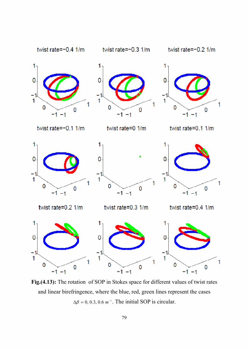
79
Fig.(4.13): The rotation of SOP in Stokes space for different values of twist rates
and linear birefringence, where the blue, red, green lines represent the cases
16.0,3.0,0 m . The initial SOP is circular.

80
Fig.(4.14): The variation of SOP for different cases of the linear birefringence and
the input SOP. The columns represent the cases of 16.0,3.0,0 m , and the rows
represent the input SOP.

81
Fig.(4.15): Changing the direction of the vector
with the effects the twist rate,
linear birefringence, and the length in Stokes space, where the colors (blue, red, and
green) represents the cases 16.0,4.0,2.0 m , respectively.

82
Fig.(4.16): The angle as a function of the twist rate for many values of lengths,
where the black, red and blue lines represent the cases of 16.0,3.0,0 m .
Fig.(4.17): The angle is a function of for many values of twist rates and L ,
where the black, blue, red, green lines represent the cases of 15.1,1,5.0,0 m .

CHAPTER FIVEConclusions and Future Works

83
CHAPTER FIVE
Conclusions and Future Works
5.1 Conclusions
The main conclusions drawn from this work are:
1. The mode coupling will exchange the power between the perpendicular axes
depending on the parameters: SOP, twist rate, fiber length and linear
birefringence, where, for any set of these parameters the coupling may be made a
certain periodic manner.
2. The probability density function for the DGD is Maxwellian for any selected
PMD factor, but the curve will be shifted more to the right for the larger PMD
factors.
3. The PMDRF is affected by L , twist rate, and fiber length. The minimum
PMDRF will be at 0 L for 0 but the increasing of will shift the
required L for higher values. This minimum PMDRF is not affected by
changing the fiber length or wavelength. But the other PMDRF values are
affected.
4. Any input SOP for the optical fiber will plot a circle around the Poincare sphere
but the operation circumstances will restrict the planes of this circle through the
operation. The type of the input SOP for the optical fiber and the related operation
circumstances may be made a random variation of the SOP on the Poincare
sphere.
5. The angle between the vector
and a certain axis is affected rapidly due to the
variation of twist rate, fiber length, and linear birefringence. This angle will be
constant for zero twist rate but for other values of twist rate it may have large
variation. However, for larger linear birefringence this angle will be approached a
certain constant.

84
5.2 Future Works
There still remains to address a lot of aspects related to the theoretical
managements that were performed in this work, such as:
1. The polarization dependent loss may be included to enhance the theoretical
view.
2. The higher order PMD effects is very important issues in the modern optical
communications, which may be analyzed to correct the resulted DGD.
3. There is a nonlinear PMD that happen due to the nonlinearity of fiber. It may
be included in the description to enhance the simulation.
4. The chromatic dispersion may be inserted in the analysis to form a unified
description of the pulse propagation in the optical fiber.
5. The spun effects may be changed the fiber birefringence. It may be used to
balance the minimum DGD.
6. The relation among the parameters: correlation length, nonlinear length,
dispersion length and pulse properties may be studied to construct the accurate
distribution of the DGD.

Appendix AThe Statistical Distribution of PMD

85
Appendix A
The Statistical Distribution of PMD
The DGD between the PSP's in a non-polarization preserving fiber is a
random variable. The DGD variations depend on the PSP's excited in the fiber, the
strain in different parts of the fiber, temperature variations, etc. For links where the
fiber is buried and undisturbed, this means that the DGD typically changes fairly
slowly [56]. We shall assume that the Cartesian components of satisfy the
relations 0)( zi and
(A.1) )(),(3
1)()( zzgjiDzz ji
where the angular brackets signify the statistical mean (or expectation) value, and
where D is a diffusion constant. The integration of stochastic differential equation
leads to [85]
(A.2) )3,2,1()()()(10
izzzdzzN
nni
z
ii
where the integral is approximated by a sum by dividing the fiber into N sections of
length z . If follows from the central limit theorem that all three components of the
PMD vector satisfy a Gaussian distribution of the form
(A.3) )2/(exp2 222/12
iiiip
The variance 2i can be found from Eq.(A.2) as
(A.4) )()()()(00
zdzzzdzzz
ki
z
ki
If we use Eq.(A.1) and carry out the indicated integrals, we obtain )()( zz ki . The
probability density function )( pmdp of the DGD can now be found using the
relation in Eq.(3.29), it can be obtained by converting the joint probability density,
)()()(),,( 321321 pppp . Clearly, individual components of the PMD vector

86
follow a Gaussian distribution, while the DGD follows the Maxwellian distribution
as shown in Fig.(A.1). From Cartesian to spherical coordinates denoted by ),,(
and integrating over the two angles, we obtain
(A.5) sin)()()()()( 2
0321
2
0
ddpppp pmd
Substituting )( ip from Eq.(A.3) and integration over the two angles produces a
factor of 4 , we obtain the Maxwellian distribution
(A.6) 2
3exp
542
2
3
2
rms
pmd
rms
pmdpmdp
The meaning of pmd is done simply as follows
(A.7) 3
8)(
0rmspmdpmdpmdpmd dp
By using Eq.(A.7), the Maxwellian distribution will take the form [42]
(A.8) 4
exp32
2
2
3
2
2
pmd
pmd
pmd
pmd
pmdp
A cursory inspection of Eq.(A.8) reveals that the )( pmdp can be found if pmd is
known.
Fig.(A.1): a) Gaussian distribution of the Stokes components of the PMD vector, b)
Maxwellian distribution of the norm of the PMD vector [5].

Appendix B
Power Splitting Ratios

87
Appendix B
Power Splitting Ratios
Consider that the PSP's occur with a uniform distribution over the Poincare
sphere, and that S is aligned with the north pole of the sphere as shown in
Fig.(B.1) [80]. The probability density of PSP's which is found in the range d
about the angle relative to S is proportional to the differential area dsin2
sketched in the figure. As there is north/south symmetry in the differential area, the
ranges (0 to π/2) and (π/2 to π) of are combined to obtain the combined
probability density sinp . For the effective range (0 to π/2) describing the
occurrence of PSP's with angle (and ) relative to S , the distribution p
is properly normalized through the range (0 to π/2). The analyses of splitting ratios
have led to a number of important fundamental advances as well as the technical
point of view. The splitting ratios can be determined from the polarization
vectors. In other words represent the projection of p| and p| onto s| .
Formally, 22 | ps , where s| and p| are the input SOP and the two
PSP's vectors [79]. If the PSP's are defined as tyx ppp | , then
(B.1) ||
||||
2
2
yxy
yxx
yx
y
x
ppp
ppppp
p
ppp
where | p are the transpose conjugation of p| . It is straightforward to show
(B.2) 1
1
1
1ˆ
132
321
132
321
2
pipp
ippp
pipp
ippppI
Using the definitions of Stokes component in Eq.(3.12), it is very easy to explain
that pIpp ˆ|| 2 . In turn, the splitting ratios can be calculated using
Eq.(B.2) and the fact that apapa ˆˆ|ˆ| as follows [42]

88
b)(B.3 2/sin2/ˆˆ12/|ˆ|||
a)(B.3 2/cos2/ˆˆ12/|ˆ|||2
22
22
2
spspIsspps
spspIsspps
Note that, the ratios are identical only for 2/ .
Fig. (B.1): differential area on Poincare sphere as a function of elevation angle [80].

References

89
References
[1] H. Dutton, " Understanding Optical Communications", First Edition,
International Technical Support Organization, IBM Corporation, USA, 1998.
[2] J. Senior and M. Jamro, " Optical Fiber Communications Principles and
Practice", Third Edition, Pearson Edition Limited, Edinburgh Gate, Harlow, Essex
CM20 2JE, England, 2009.
[3] G. Agrawal, " Fiber-Optic Commnunication Systems", Third Edition, John
Wiley& Sons, Inc., Rochester, Ny, 2002.
[4] D.Bailey and E. Wright, " Practical Fiber Optics", Elsevier, 2003.
[5] G. Agrawal, " Lightwave Technology", Wiley-Interscience, 2005.
[6] M. Reimer, " Modeling and Simulation of Polarization Mode dispersion and
Polarization Dependent Loss", M. Sc. Thesis, University of Waterloo, 2007.
[7] M. Ferreira, " Nonlinear Effects in Optical Fibers", Wiley, 2011.
[8] L. Nelson and R. Jopson, " Introduction to Polarization Mode Dispersion in
Optical Systems", Chapter in the book "Polarization Mode Dispersion", Edited by
C. Menyuk and A. Galtarossa, Springer, 2005.
[9] A. Galtarossa and L. Palmieri, " Reflectometric Measrurements of Polarization
Properties in Optical-Fiber Links", Chapter in the book "Polarization Mode
Dispersion", Edited by C. Menyuk and A. Galtarossa, Springer, 2005.
[10] G. Agrawal, " Nonlinear Fiber Optics", Academic Press, Forth Edition, 2007.
[11] C. Chen, " Foundations for Guided-Wave Optics", Wiley-Interscience, 2007.
[12] L. Cohen, B. Hille and R. Keynes, " Changes in Axon Birefringence During
The Action Potential", J. Physiol, 211, 1970.
[13] D. Gloge, " Bending Loss in Multimode Fibers with Graded and Ungraded
Core Index", Applied Optics, Vol. 11, No. 11, 1972.
[14] W. Gambling and H. Matsumura, " Pulse Response of a Graded-Index Optical
Fiber", Electronics Letters, Vol. 9, No. 15, 1973.

90
[15] D. Marcuse and H. Presby, " Mode Coupling in an Optical Fiber with Core
Distortions", The Bell System Technical Journal, Vol. 54, No. 1, 1975.
[16] D. Marcuse, " Microbending Losses of Single-Mode, Step-Index and
Multimode, Parabolic-Index Fibers" The Bell System Technical Journal, Vol. 55,
No. 7, 1976.
[17] M. Adams, D. Payne and C. Ragdale, " Birefringence in Optical Fibers with
Elliptical Cross-Section ", Electronics Letters, Vol. 15, No. 10, 1979.
[18] H. Sunak and J. Neto, " Intermodal Pulse Dispersion in Multimode Optical
Fibers and Its Measurement with a Nanosecond Test Facility", Revista Brasileira
De Fisica, Vol. 10, No. 3, 1980.
[19] A. Barlow, J. Ramskov-Hansen and D. Payne, " Birefringence and
Polarization Mode-Dispersion Spun Single-Mode Fibers", Applied Optics, Vol. 20,
No. 17, 1981.
[20] J. Sakai and T. Kimura, " Birefringence and Polarization Chracteristics of
Single-Mode Optical Fibers Under Elastic Deformations", IEEE, Vol. 17, No. 6,
1981.
[21] D. Payne, A. Barlow and J. Hansen, " Development of Low-and High-
Birefringence Optical Fibers", IEEE Journal of Quantum Electronics, Vol. 18, No.
4, 1982.
[22] I. White and S. Mettler, " Modal Analysis of Loss and Mixing in Multimode
Parabolic Index Splices", The Bell System Technical Journal, Vol. 62, No. 5, 1983.
[23] C. Tsao, " Polarization Parameters of Plane Waves in Hybrid birefringent
Optical Fibers", Journal of Optical Society of America A, Vol.4, Page 1407, 1987.
[24] C. Shi and R. Hui, " Polarization Coupling in Single-Mode Single-Polarization
Optical Fibers", Optics Letters, Vol. 13, No. 12, 1988.

91
[25] S. Poole, J. Townsend, D. Payne, M. Fermann, G. Cowle, R. Laming, and P.
Morkel, " Characterization of Special Fibers and Fiber Devices", Journal of
Lightwave Technology, Vol. 7, No. 8, 1989.
[26] N. Gisin, J. Weid, and J. Pellaux, " Polarization Mode Dispersion of Short and
Long Single-Mode Fibers", Journal of Lightwave Technology, Vol. 9, No. 7, 1991.
[27] C. Poole and T. Darcie, " Distortion Related to Polarization-Mode Dispersion
in Analog Lightwave Systems", Journal of Lightwave Technology, Vol. 11, No. 11,
1993.
[28] P. Wai and C. Menyuk, " Polarization Mode Dispersion, Decorrelation, and
Diffusion in Optical Fibers with Randomly Varying Birefringence", Journal of
Lightwave Technology, Vol. 14, No. 2, 1996.
[29] A. Galtarossa, L. Palmieri, M. Schiano and T. Tambosso, " Statistical
Characterization of Fiber Random Birefringence", Optics Letters, Vol. 25, No. 18,
2000.
[30] I. Lima, R. Khosravani, P. Ebrahimi, E. Ibraimov, C. Menyuk, and A. Willner,
" Comparison of Polarization Mode Dispersion Emulators", Journal of Lightwave
Technology, Vol. 19, No. 12, 2001.
[31] Y. Tan, J. Yang, W. Kath and C. Menyuk, " Transient Evolution of the
Polarization-Dispersion Vector's Probability Distribution", J. Opt. Soc. Am. B, Vol.
19, No. 5, 2002.
[32] A. Galtarossa, L. Palmieri, A. Pizzinat, B. Marks, and C. Menyuk, " An
Analytical Formula for the Mean Differential Group Delay of Randomly
Birefringent Spun Fibers", Journal of Lightwave Technology, Vol. 21, No. 7, 2003.
[33] D. Nolan, X. Chen, and Ming-Jun Li, " Fibers With Low Polarization-Mode
Dispersion ", Journal of Lightwave Technology, Vol. 22, No. 4, 2004.
[34] L. Yan, M. Hauer, Y. Shi, X. Yao, P. Ebrahimi, Y. Wang, A. Willner, and W.
Kath, " Polarization-Mode-Dispersion Emulator Using Variable Differential-

92
Group-Delay (DGD) Elements and Its Use for Experimental Importance
Sampling", Journal of Lightwave Technology, Vol. 22, No. 4, 2004.
[35] X. Chen, M. Li, and D. Nolan, " Polarization Evolution in Spun Fibers", Proc.
Of SPIE, Vol. 6019 ,60192J, 2005.
[36] H. Yasser, " Pulse Broadening Due to Polarization Mode Dispersion and
Chromatic Dispersion in Optical Fiber Communications", Journal of Thi-Qar
University, Vol. 2, No. 1, 2006.
[37] L. Yan, X. Yao, M. Hauer, and A. Willner, " Practical Solutions to
Polarization-Mode-Dispersion Emulation and Compensation", Journal of
Lightwave Technology, Vol. 24, No. 11, 2006.
[38] J. Lee, " Analysis of the Polarization-Mode-Dispersion Vector Distribution for
Linearly Birefringent Optical Fibers", IEEE Photonics Technology Letters, Vol. 19,
No. 13, 2007.
[39] Z. Li, C. Wu, H. Dong, P. Shum, C. Tian, and S. Zhao, " Stress Distribution
and Induced Birefringence Analysis for Pressure Vector Sensing Based on Single
Mode Fibers", Optics Express, Vol. 16, No. 6, 2008.
[40] T. Xu, F. Tang, W. Jing, H. Zhang, D. Jia, X. Zhang, G. Zhang, G. Zhou, Y.
Zhang, " Distributed Measurement of Mode Coupling in Birefringent Fibers with
Random Polarization Modes", Optica Applicata, Vol. XXXIX, No. 1, 2009.
[41] H. Wen, M. Terrel, H. Kim, M. Digonnet, and S. Fan, " Measurements of the
Birefringence and Verdet Constant in an Air-Core Fiber", Journal of Lightwave
Technology, Vol. 27, No. 15, 2009.
[42] H. Yasser, " Statistical Model for Polarization Mode dispersion in single Mode
fibers", Baghdad Science Journal, Vol. 7(3), 2010.
[43] A. Mafi, P. Hofmann, C. Salvin, and A. Schulzgen, " Low-Loss Coupling
Between Two Single-Mode Optical Fibers with Different Mode-Field Diameters

93
Using A graded-Index Multimode Optical Fibr", Optics Letters, Vol. 36, No. 18,
2011.
[44] I. Khan, " Jones Matrix Method: An Analytical Approach to Study Light
Transmission Through Optical Materials", Canadian Journal on Electrical and
Electronics Engineering, Vol. 3, No. 10, 2012.
[45] H. Yasser and N. Shnan, " Evolution of Random Vectors Along Single-Mode
Fiber in Presence of Conventional Polarization Effects", Journal of Babylon
University/ Pure and Applied Sciences, Vol. 21, No. 7, 2013.
[46] D. Tentori and A. Weidner, " Jones Birefringence in Twisted Single-Mode
Optical Fibers", Optics Express, Vol. 21, No. 26, 2013.
[47] G. Pal and M. Gupta, " Signal Degradation in Optical Fibers", International
Journal of Emerging Technologies and Engineering (IJETE), Vol. 1, No. 1, 2014.
[48] M. Yamanari, S. Tsuda, T. Kokubun, Y. Shiga, K. Omodaka, Y. Yokoyama,
N. Himori, M. Ryu, S. Sanuki, H. Takahashi, K. Maruyama, H. Kunikata, and T.
Nakazawa, " Fiber-Based Polarization-Sensitive OCT for Birefringence Imaging of
the Anterior Eye Segment", Biomedical Optics Express, Vol. 6, No. 2, 2015.
[49] E. Awad, " Basics of Fiber Optics", Chapter 2 in, " Fiber Optics", T. Manual,
Second Edition, 2001.
[50] P. Lecoy, " Fiber-Optic Communications", Wiley, 2008.
[51] J. Laferriere , G. Lietaert, R. Taws and S. Wolszczak, " Reference Guide to
Fiber Optic Testing", Second Edition, JDSU, 2011.
[52] S. Gistvik, " Optical Fiber Theory for Communication Networks", Second
Edition, Ericsson Network Technologies AB Hudiksvall Sweden, 2002.
[53] R. Tricker, " Optoelectronics and Fiber Optic Technology", Elsevier, 2002.
[54] B. Woodward and E. Husson, " Fiber Optics Installer and Technician Guide",
SYBEX, 2005.

94
[55] F. Mitschke, " Fiber Optics Physics and Technology", Springer-Verlag, Berlin,
Heidelberg, Germany, 2009.
[56] M. Johnson, " Optical Fiber, Cables and Systems", ITU, 2009.
[57] K. Thyagarajan and A. Ghatak, " Fiber Optic Essentials", John Wiley& Sons,
Inc, 2007.
[58] A. Kumar and A. Chatak, " Polarization of Light with Application in Optical
Fibers", SPIE, 2011.
[59] M. Marhic, " Fiber Optical Parametric Amplifiers, Oscillators and Related
Devices", Cambridge University Press, 2008.
[60] B. Elliott and M. Gilmore, " Fiber Optic Cabling", Second Edition, Newnes,
2002.
[61] U. Osterberg, " Optical Fiber, Cable, and Connectors", Chapter 1 in
"Handbook of Fiber Optic Data Communication", Second Edition, Edited by C.
Decusatis, Academic Press, 2002.
[62] P. Kondamuri, " Characterization of Polarization-Mode Dispersion on Buried
Standard Single-Mode Fibers", M.Sc. Thesis, University of Kansas, Faculty of The
Graduate Schoole, 2000.
[63] G. Agrawal, " Applications of Nonlinear Fiber Optics", Academic Press, 2001.
[64] J. Gordon and H. Kogelnik, " PMD Fundamentals: Polarization Mode
Dispersion in Optical Fibers", Proceedings of the National Academy of Sciences,
Vol. 97, No. 9, 2000.
[65] H. Yasser and M. Saheb, " Theoretical Comparison Between Polarization
Mode Dispersion and Birefringence Vectors in Single Mode Fibers", Journal of
University of Thi-Qar, Vol. 2, No. 2, 2006.
[66] F. Dai, " Electronic Equalizations for Optical Fiber Dispersion
Compensation", SPIE, Vol. 46, No. 3, 2007.

95
[67] A. Yariv and P. Yeh, " Photonics Optical Electronics in Modern
Communications", Sixth Edition, Oxford University Press, 2007.
[68] M. Cada, " Active Optical Waveguides", Chapter 4 in "Optical Waveguides
From Theory to Applied Technologies", Edited by M. Calvo and V.
Lakshmiuarayanan, CRC Press, Taylor & Francis Group, 2007.
[69] Y. Kivshar and G. Agrawal, " Optical Solitons From Fibers to Photonic
Crystals", Academic Press, 2003.
[70] S. Namiki, Y. Emori, and A. Oguri, " Discrete Raman Amplifiers", Chapter 4
in "Raman Amplification in Fiber Optical Communication Systems", Edited by C.
Headley and G. Agrawal, , Elsevier Academic Press, 2005.
[71] C. Poole and J. Nagel, " Polarization Effects in Lightwave Systems", Chapter
6 in "Optical Fiber Telecommunications", IIIA, Edited by I. Kaminow and T.
Koch, , Academic Press, Lucent Technologies, 1997.
[72] P. Prasad, " Investigation of optical Multi Input Multi Output (OMIMO)
Transmission Link Using Multimode Fiber", M. Sc. Thesis, Thapar University,
2013.
[73] R. Schuh, " Characterisation of Birefringence in Optical Fibers", Ph.D. Thesis,
Department of Electronic Systems Engineering, University of Essex, 1997.
[74] A. Rogers, " Polarization in Optical Fibers", Artech House, 2008.
[75] A. Ghatak and K. Thyagarajah, " Introduction to Fiber Optics", Cambridge
University Press, 1997.
[76] W. Huang, " Fiber Birefringence Modeling for Polarization Mode Dispersion",
Ph.D. Thesis, University of Waterloo, 2007.
[77] P. Drexler and P. Fiala, " Optical Fiber Birefringence Effects-Sources,
Utilization and Methods of Suppression", Chapter 7 in "Recent Progress in Optical
Fiber Research", Edited by M. Yasin, S. Harun and H. Arof, , InTech, 2011.

96
[78] Y. Tan, J. Yang, W. Kath and C. Menyuk, " Transient Evolution of the
Polarization Dispersion Vectors Probability Distribution", J. Opt. Soc. Am. B, Vol.
19, No. 5, 2002.
[79] H. Yasser, " Polarization Losses in Optical Fibers", InTech, 2012.
[80] N. Al-Zubaidi, " Performance of Single Mode Fiber System in Presence the
Conventional Polarization Effects", Ph. D. Thesis, University of Al-
Mustansiriyahin , College of Education, 2013.
[81] S. Sundhararajan, " In Situ PMD Monitoring Using Coherent Detection and
Polarization Tracking", M. Sc. Thesis, Faculty of the Graduate School of the
University of Kansas, 2008.
[82] P. Sundsqy, " Depolarization of Orthogonal States of Polarization in Fiber
Optic High-Speed Transmission", M. Sc. Thesis, Norwegian University of Science
and Technology, 2004.
[83] L. Cherbi and A. Bellil, " Spun Fibers for Compensation of PMD: Theory and
Characterization", Chapter 8 in " Recent Progress in Optical Fiber Research",
Edited by M. Yasin, S. Harun and H. Arof, , InTech, 2011.
[84] P. Lesiak and T. Wolinski, " Simultaneous Twist and Longitudinal Strain
Effects on Polarization Mode Dispersion in Highly Birefringent Fibers", Opto-
Electronics Review, Vol. 13, No. 2, 2005.
[85] J. Gordon, " Statistical Properties of Polarization Mode Dispersion", Chapter
in the book "Polarization Mode Dispersion", Edited by C. Menyuk and A.
Galtarossa, Springer, 2005.

الخالصة
على خواص النبضات المنتشرة فعاالا برزت ظاھرة تشتت نمط االستقطاب بوصفھا مؤثر
ثانیة الن مقدار / في األلیاف البصریة بعد زیادة نسب اإلرسال إلى حدود تجاوزت عدة تیرا بایت
صلي وھذا یعني بالمقارنة مع عرض النبضة األصبح كبیراض الذي تتعرض لھ النبضة یالتعری
.مسموح بھا إلى نظام اإلرسالإضافة أخطاء غیر
. اور المتعامدةللمحالمزدوجاالنكسارظاھرة إن أساس ظاھرة تشتت نمط االستقطاب ھو
وتبعا لذلك یتم تحلیل النظام ریاضیا ظاھرة خطیةفي اغلب األحیان یعتبر إن االنكسار المزدوج
ظاھرة البرم للیف البصري فاناألخذ بنظر االعتبار تأثیرعند.لتحدید خواص النبضات الناتجة
اقتران النمط، مركبة : تبعا لذلك سوف یتغیر كل من. المزدوج تصبح ال خطیةاالنكسار
.االستقطاب ونسبة تعریض النبضة
ووفقا لذلك تم اشتقاق صیغ في ھذا البحث، تم إضافة تأثیر البرم إلى متجھ ثنائي االنكسار
ھذه التعابیر . اقتران النمط، مركبة االستقطاب ونسبة تعریض النبضة: صف كل منلوریاضیة
أثبتت النتائج إن اقتران النمط یتأثر . تؤول إلى الصیغ الریاضیة المعروفة بعد إسقاط تأثیر البرم
. مقدار ثنائي االنكسار الخطي ونسبة البرم، حالة االستقطاب الداخل، طول اللیف: كثیرا بكل من
.لوك الدوري لتبادل القدرة على المحورین یحدد باختیار معین لتلك المؤثراتالس
ر لحالة االستقطاب حدوث تدویبة االستقطاب في فضاء ستوكسمركأثبتت، من جانب أخر
تعریض النبضة الناتج بوجود التأثیرات المذكورة یمكن إن یقلل . العوامل السابقةبقدر یعتمد على
لظاھرة االنكسار الخطیة والدائریةالتأثیرات إلى اقل قدر وربما صفر باالعتماد على الموازنة بین
حیث إن ھذه الموازنة ال تعتمد على طول اللیف أو الطول ألموجي المستعمل عندما ، المزدوج
وطالما إننا نسعى في وجود البرم إلى إلغاء . األمر بتحقیق اقل عرض ممكن للنبضةیتعلق
. یماثل التوزیعات التقلیدیةتوزیع اإلحصائي لمقدار التعریض التعریض النبضة الناتج فان ال

العراقجمھوریة
العلميوالبحثالعاليالتعلیموزارة
العلومكلیة-قارذيجامعة
قسم الفیزیاء
واقتران النمطتقدم االستقطاب لدراسة نظریة
منفردة النمطالالبصریة المفتولة األلیاففي
إلىمقدمةرسالة
منجزءوھيقارذيجامعةفيالعلومكلیةمجلس
الفیزیاءعلومفيالماجستیردرجةنیلمتطلبات
من قبل
نور علي ناصرفیزیاءالعلوم/ علومبكالوریوس
٢٠١٣
شرافإ
حسن عبد یاسر. د. أھــ١٤٣٧ م ٢٠١٥
CHكج