Embed Size (px)
Citation preview
THEORETICAL INVESTIGATIONS OF TERASCALE PHYSICS
by
WEI GONG
A DISSERTATION
Presented to the Department of Physicsand the Graduate School of the University of Oregon
in partial fulfillment of the requirementsfor the degree of
Doctor of Philosophy
September 2()09- -

11
University of Oregon Graduate School
Confirmation of Approval and Acceptance of Dissertation prepared by:
Wei Gong
Title:
"Theoretical Investigations of Terascale Physics"
This dissertation has been accepted and approved in partial fulfillment of the requirements forthe Doctor of Philosophy degree in the Department of Physics by:
Stephen Hsu, Chairperson, PhysicsGraham Kribs, Member, PhysicsDavid Strom, Member, PhysicsDavison Soper, Member, PhysicsMarina Guenza, Outside Member, Chemistry
and Richard Linton, Vice President for Research and Graduate Studies/Dean of the GraduateSchool for the University of Oregon.
September 5, 2009
Original approval signatures are on file with the Graduate School and the University of OregonLibraries.
III
An Abstract of the Dissertation of
Wei Gong for the degree of Doctor of Philosophy
in the Department of Physics to be taken September 2009
Title: THEORETICAL INVESTIGATIONS OF TERASCALE PHYSICS
Approved:Dr. Davison E. Soper
In this dissertation, three different topics related to terascale physics are explored.
First, a new method is suggested to match next-to-Ieading order (NLO) scattering
matrix elements with parton showers. This method is based on the original approach
which adds primary parton splittings in Born-level Feynman graphs in order to
remove several types of infrared divergent subtractions from the NLO calculation.
The original splitting functions are modified so that parton showering has a less
severe effect on the jet structure of the generated events.
We also examine the Large Hadron Collider phenomenology of quantum black
holes in models of TeV scale gravity. Based on a few minimal assumptions, such as
the conservation of color charges, interesting signatures are identified that should be
readily visible above the Standard Model background. The detailed phenomenology
depends heavily on whether one requires a Lorentz invariant, low-energy effective
field theory description of black hole processes.
Finally, in the calculation of cross sections in high energy collisions at NLO, one
option is to perform all of the integrations, including the virtual loop integration,
by Monte Carlo numerical integration. A new method is developed to perform the
loop integration directly, without introducing Feynman parameters, after suitably
iv
deforming the integration contour. Our example is the N-photon scattering amplitude
with a massless electron loop. Results for six photons and eight photons are reported.
CURRICULUM VITAE
NAME OF AUTHOR: Wei Gong
PLACE OF BIRTH: Chengdu, Sichuan, China
DATE OF BIRTH: June, 1981
GRADUATE AND UNDERGRADUATE SCHOOLS ATTENDED:
University of Oregon, Eugene, Oregon, USAUniversity of Science and Technology of China, Hefei, China
DEGREES AWARDED:
Doctor of Philosophy in Physics, 2009, University of OregonBachelor of Science in Physics, 2004, University of Science and
Technology of China
AREAS OF SPECIAL INTEREST:
Standard Model phenomenologyMonte Carlo algorithms
PROFESSIONAL EXPERIENCE:
Research assistant, Institute of Theoretical Science, University ofOregon, 2005-2009
Teaching assistant, Dept. of Physics, University of Oregon, 2004-2009
v
PUBLICATIONS:
Wei Gong, Zoltan Nagy, and Davison E. Soper, "Direct numericalintegration of one-loop Feynman diagrams for N-photon amplitudes" ,Phys. Rev. D79:033005 (2009).
Xavier Calmet, Wei Gong, and Stephen D.H. Hsu, "Colorful quantumblack holes at the LHC", Phys. Lett. B668:20-23 (2008).
vi

vii
ACKNOWLEDGMENTS
I would like to thank my advisor Professor Davison Soper, who has always been
there to help me to study as a scientist and to grow as an individual. Thank you
for your constant encouragement, support and guidance. I have benefited so much
from being your student for four years, and there are not enough words for me to
express my gratitude. I would also like to thank Professor Stephen Hsu for countless
helpful discussions during our collaborative research, and for his incisive thoughts
and expertise outside the academic field which eventually enabled me to have the
opportunity to launch my career in the business world. I want to acknowledge
and thank Professor Graham Kribs, Professor Nilendra Deshpande and Dr. Xavier
Calmet as well, for their helpful hints and advice along my way of pursuing the
doctorate degree.
I want to thank my peers in the Institute of Theoretical Science, David Reeb,
Ricky Fok, Tuhin Roy, and my former officemate Andrew Cook. I have learned so
much from the many discussions with you. I also want to thank all the other faculty
members, students and staff of the Department of Physics - you always make me feel
at home although I am thousands miles away from where I came from. I wish you
well in all that you do.
I am extremely fortunate to have a wonderful and caring family. To my mom,
Jun Miao, my dad, Xiangjin Gong, and grandparents, aunts, uncles and cousins
thank you all for your love and support for so many years. I would not be able to
achieve anything in my life without your belief in me.
And at last, but not in the least, I want to thank the most important person in
my life, the sweetest person in the world, my lovely wife, Lei. You are my partner,
Vlll
my best friend, and so much more. I can never thank you enough for all that you
have done for me. I love you from the bottom of my heart.

To my wife - Lei Zhang - you keep my dream alive.
IX
TABLE OF CONTENTS
Chapter
1. INTRODUCTION
II. NLO CALCULATION AND PARTON SHOWERS
2.1 Introduction ....2.2 Event Generator ..2.3 Pure NLO Program2.4 Parton Evolution. .
2.4.1 Introduction.2.4.2 Splitting Functions2.4.3 Parton Evolution2.4.4 Implementation.
2.5 Adding Parton Showers2.5.1 Motivation .,.2.5.2 Implementation.2.5.3 Numerical Tests.2.5.4 Manipulation of Splitting Functions.
2.6 Event Shape Variables .2.6.1 Jet Algorithms .2.6.2 Thrust-Related Variables2.6.3 C-Parameter .2.6.4 Spherocity. . . . . . . . .2.6.5 Energy-Energy Correlation Function
2.7 Numerical Results .2.7.1 Validating Numerical Results2.7.2 Numerical Convergence ...
III. COLORFUL QUANTUM BLACK HOLES.
3.1 Introduction .
x
Page
1
3
349
14141529374040465660646565697072747492
98
98
Chapter
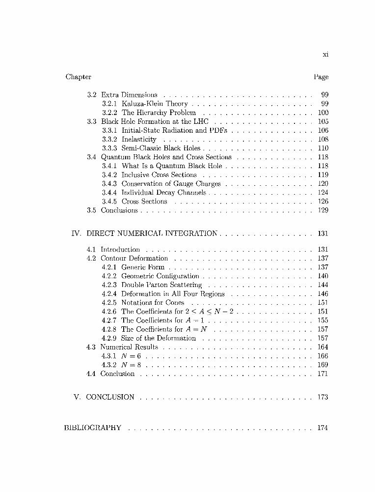
3.2 Extra Dimensions .3.2.1 Kaluza-Klein Theory ..3.2.2 The Hierarchy Problem
3.3 Black Hole Formation at the LHC3.3.1 Initial-State Radiation and PDFs3.3.2 Inelasticity .3.3.3 Semi-Classic Black Holes. . . . .
3.4 Quantum Black Holes and Cross Sections3.4.1 What Is a Quantum Black Hole .3.4.2 Inclusive Cross Sections ....3.4.3 Conservation of Gauge Charges3.4.4 Individual Decay Channels.3.4.5 Cross Sections
3.5 Conclusions. . . . . . . . . . . . .
IV. DIRECT NUMERICAL INTEGRATION.
4.1 Introduction .....4.2 Contour Deformation
4.2.1 Generic Form .4.2.2 Geometric Configuration.4.2.3 Double Parton Scattering4.2.4 Deformation in All Four Regions4.2.5 Notations for Cones .4.2.6 The Coefficients for 2 ~ A ~ N - 24.2.7 The Coefficients for A = 1 .4.2.8 The Coefficients for A = N4.2.9 Size of the Deformation
4.3 Numerical Results4.3.1 N = 64.3.2 N = 8
4.4 Conclusion
Xl
Page
9999
100105106108110118118119120124126129
131
131137137140144146151151155157157164166169171
V. CONCLUSION . . . . . . . . . . . . . . . . . . . . . . . . . . . . . . . 173
BIBLIOGRAPHY 174

LIST OF FIGURES
Figure
2.1 Jet mass distribution .
2.2 Cancellation between infrared divergences
2.3 Jet mass distribution by PYTHIA ....
2.4 Kinematics of timelike parton branching.
2.5 Gluon splitting into gluons .
2.6 Gluon splitting into quark-antiquark .
2.7 Quark splitting into gluon and quark
2.8 Illustration of the evolution operator .
2.9 NLO graphs that contributes to divergences.
2.10 Cut propagators ..
2.11 Shower propagator .
2.12 Deleting cut NLO graphs
2.13 Proposal function ....
2.14 Validating NLO calculation with showers
2.15 Jet mass distribution in the full NLO+PS+Had calculation
2.16 Distribution of jet masses
2.17 Three jet fraction ....
2.18 Three jet fraction with a modified splitting function
2.19 Thrust for pure NLO (91 GeV) .
xii
Page
11
12
13
15
17
20
23
34
40
41
45
45
51
57
59
59
60
63
75

Xlll
Figure Page
2.20 Thrust for pure NLO (35 GeV) ........ 76
2.21 Thrust with old splitting functions (91 GeV) 76
2.22 Thrust with old splitting functions (35 GeV) 77
2.23 Thrust with modified splitting functions (91 GeV) 77
2.24 Thrust with modified splitting functions (35 GeV) 78
2.25 C-Parameter for pure NLO (91 GeV) 78
2.26 C-Parameter for pure NLO (35 GeV) 79
2.27 C-Parameter with old splitting functions (91 GeV) 79
2.28 C-Parameter with old splitting functions (35 GeV) 80
2.29 C-Parameter with modified splitting functions (91 GeV) 80
2.30 C-Parameter with modified splitting functions (35 GeV) 81
2.31 Heavy Jet Mass for pure NLO (91 GeV) . 81
2.32 Heavy Jet Mass for pure NLO (35 GeV) . 82
2.33 Heavy Jet Mass with old splitting functions (91 GeV) 82
2.34 Heavy Jet Mass with old splitting functions (35 GeV) 83
2.35 Heavy Jet Mass with modified splitting functions (91 GeV) 84
2.36 Heavy Jet Mass with modified splitting functions (35 GeV) 84
2.37 Total Jet Broadening for pure NLO (91 GeV) . 85
2.38 Total Jet Broadening for pure NLO (35 GeV) . 85
2.39 Total Jet Broadening with old splitting functions (91 GeV) 86
2.40 Total Jet Broadening with old splitting functions (35 GeV) 86
2.41 Total Jet Broadening with modified splitting functions (91 GeV) 87
xiv
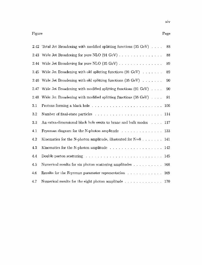
2.42 Total Jet Broadening with modified splitting functions (35 GeV) 88
2.43 Wide Jet Broadening for pure NLO (91 GeV) . 88
2.44 Wide Jet Broadening for pure NLO (35 GeV) . 89
2.45 Wide Jet Broadening with old splitting functions (91 GeV) 89
2.46 Wide Jet Broadening with old splitting functions (35 GeV) 90
2.47 Wide Jet Broadening with modified splitting functions (91 GeV) 90
2.48 Wide Jet Broadening with modified splitting functions (35 GeV) 91
3.1 Protons forming a black hole . 106
3.2 Number of final-state particles 114
3.3 An extra-dimensional black hole emits to brane and bulk modes 117
4.1 Feynman diagram for the N-photon amplitude . . . . . . . . 133
4.2 Kinematics for the N-photon amplitude, illustrated for N=8 . 141
4.3 Kinematics for the N-photon amplitude 142
4.4 Double parton scattering . . . . . . . . 145
4.5 Numerical results for six photon scattering amplitudes 168
4.6 Results for the Feynman parameter representation 169
4.7 Numerical results for the eight photon amplitude . 170
LIST OF TABLES
xv
Table Page
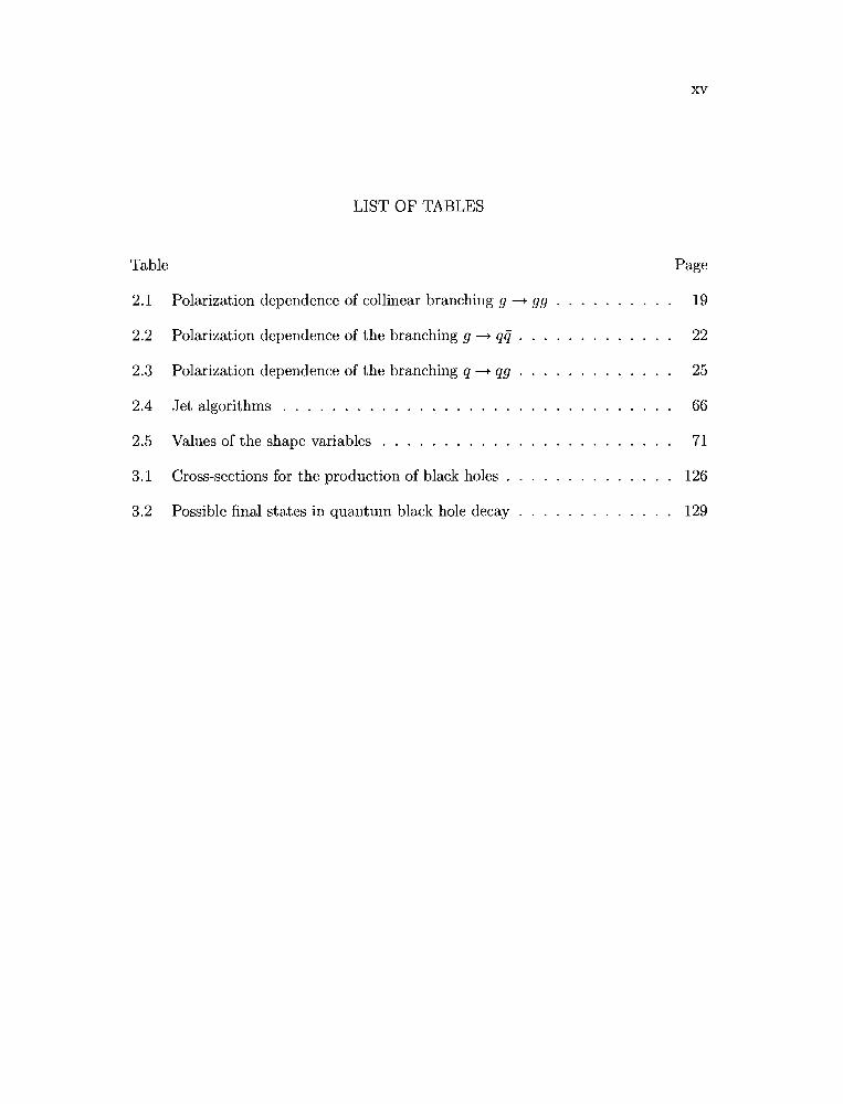
2.1 Polarization dependence of collinear branching 9 --+ gg 19
2.2 Polarization dependence of the branching 9 --+ qq . 22
2.3 Polarization dependence of the branching q --+ qg 25
2.4 Jet algorithms ........ 66
2.5 Values of the shape variables 71
3.1 Cross-sections for the production of black holes 126
3.2 Possible final states in quantum black hole decay 129
1
CHAPTER I
INTRODUCTION
The Large Hadron Collider (LHC) has been built in Geneva, Switzerland, which
will enable us to probe the fundamental building blocks of our universe at a
unprecedented energy scale. In this collider, protons beams will be smashed together
at a center-of-mass energy of 14 tera electron volts (TeV). In such a regime, it is
believed by many that new physics beyond the Standard Model will emerge. A large
number of theoretical models have been developed to resolve some open problems
that remain in the Standard Model, and those new theories can predict what new
could possibly come out of the LHC. For example, some suggest there are extra
dimensions in addition to the oridinary 4 spacetime dimensions, which might lower
the fundamental scale of gravity and give rise to the production of mini black holes.
In this dissertation, we will discuss the phenomenology of such black holes whose size
is even smaller than that of a proton.
Many experiments need to be performed at the LHC to test the validity of those
new physics theories. Any of such theories will be strongly supported if some of its
unique signatures can be identified above the Standard Model background. As a
result, it is important for us to improve both the accuracy and efficiency of numerical
calculations based on the Standard Model, so that interesting signatures for Terascale
physics could more easily be observed. For this purpose, we will investigate two other
topics in this dissertation. One of them is about matching next-to-Ieading order
(NLO) scattering matrix elements with parton showers using primary splittings, and
the other is about the direct numerical integration of virtual loop Feynman diagram
with multiple external legs.

2
This dissertation will first introduce our method to match NLO calculation with
parton showers. Following that, we will cover the phenomenology of quantum black
holes at the LHC. Finally, the direct numerical integration of virtual loop graphs will
be discussed.
3
CHAPTER II
NLO CALCULATION AND PARTON SHOWERS
2.1 Introduction
Perturbation theory is one of the most powerful tools when it comes to predicting
various aspects of possible outcome of elementary particle experiments. Monte Carlo
(MC) event generators have been built as an application of the perturbation theory
of the standard model of elementary particle physics. They can produce final-state
events according to fundamental theories like Quantum Electro Dynamics (QED) and
Quantum Chromo Dynamics (QCD). People can match the simulated events with
realistic events from lab experiments by comparing properties like cross sections,
event shape, and other observables. Through tuning those input parameters in the
standard model, for example, the strong coupling constant as, people are able to find
out how good the match can be, and thus evaluate the theories behind the particle
model. Specifically, when strong interactions are involved, MC event generators can
be created based upon perturbative QCD calculation. But we can not carry out
sensible perturbative calculations of QCD unless there is large momentum transfer
or short-distance interaction. The reason is in order to make perturbation theory
work properly, the strong coupling constant has to be small because the results
are usually expanded in powers of as(Q). And for a non-Abelian theory, QCD,
the strong coupling constant will decrease as the energy scale Q of the process
increases. This phenomena is known as "asymptotic freedom". Approximately
speaking, it would make sense for people to use the perturbative approach to tackle
problems with strong interactions only when Q is much bigger than 1 GeV. People
4
can also choose to measure only "infrared-safe" observables to exclude most of the
low scale effects like hadronization. On the other hand, those well accepted MC
event generators today can only do leading-order calculations, and contributions
from higher order perturbative terms can make those generators heavily depend on
the input renormalization scale of the programs. It will be necessary to include
the next-to-leading order terms or even higher order effects in the event generator
so that one can deal with more advanced experiments like those in the upcoming
Large Hadron Collider (LHC). I have done a project that focuses on how to match
parton showers to pure next-to-leading Order (NLO) computations, which is the key
to developing a MC event generator accurate to NLO in QCD.
2.2 Event Generator
People usually make up observables to describe the shape of events. For example,
F can be a function of final-state momenta, and we use the following formula to
calculate an observable based upon this function [1],
(j[F] = L ~JdPI ... din d - d(j d _ x Fn (PI,' .. ,in)· (2.1)n n. Pl'" Pn
In the above expression, Pi is the final-state momentum, d(j / dPI ... din is the cross
section to make n massless partons. For the purpose of this article, all n partons
are treated as identical when defining the cross section and therefore we divide by
a factor of n!, because we can intentionally construct function F to be independent
of flavor and color of final-state partons, and symmetric under interchange of any of
parton momenta.
F also needs to be infrared-safe as well, but what exactly is the so-called "infrared
safety"? If a certain function F meets the criteria mentioned above, and if in the limit
where two partons become collinear, or one becomes soft, it also has the following
property [2]:
(2.2)
5
then this function is infrared safe.
There are a few reasons for people to use infrared safe observables to probe
processes like e+e- --t hadrons. One of them is that a lot of long distance effects
cannot be calculated accurately. For example, there is no model in which final
state partons can evolve through the stage of hadronization numerically, because at
this low energy scale, as predicted by non-Abelian gauge theory, the strong coupling
constant as has become so big that perturbation theory breaks down. Thus in current
QeD event generators, hadronization can only be realized with the help of various
phenomenological models, and those models can introduce systematic errors, with
their sizes not clearly known. However, compared to the hard part of the scattering
process, two interacting particles during the hadronization stage can be treated as
being either collinear with each other or one being soft. Therefore, a well-constructed
infrared safe observable can measure the hard scattering matrix elements precisely,
while being very insensitive to uncertainties brought by our choice of hadronization
models.
Another reason for us to stick to infrared safe observables is, when people use
equation (2.1) to calculate a-[F]' there are infrared divergences which will cancel
between terms with difference number of partons. In order to make sure the
cancellation works correctly, functions of difference parton numbers have to be related
in the way set by equation (2.2).
It should be helpful to briefly show the origin of those divergence present in the
infrared region. Let us take quark splitting into a quark-gluon pair as an example.
Assume that the two daughter partons are both on-shell. For the daughter quark,
this means q2 = m 2; and for the daughter gluon, this means p2 = O. If there is no
quark flavor change during the splitting, and assuming 1t11 = zEq where 0 < z < 1,

6
then the denominator of the mother quark's propagator would be
(q + p)2 _ m2 = (q2 _ m2) + p2 + 2 (p. q)
= 2 (p. q)
= 2Ep Eq (1 - z cos B) , (2.3)
where B is the angle between two daughter partons. For the numerator factor of this
same propagator, it turns out to contain a factor of B in the collinear limit. Then
apparently, at high energy when z ----t 1, the squared matrix element including this
splitting process is approximated by
(2.4)
when B ----t O. Then, the cross section
(2.5)
can apparently become divergent as the two daughter partons go collinear or the
gluon gets very soft. However, if we include another graph of the same order, but
with a virtual loop in place of the splitting, then the infrared singularity that appeared
above would be cancelled by another singularity provided by this newly added graph.
Now I will start to explain how to use a typical event generator to calculate such an
observable. Usually, many events will pop out of the event generator, with a certain
weight factor Wi assigned to each event, which plays the role of the cross section of
events with the corresponding final-state momentum configuration. However, some
event generators would sometimes give negative weights [2]. The observable will be
calculated in the way given below:
N
[ ] _ ~ '"' . ({i} {i} {i})(J" F - N D w~F PI , P2 , ... ,Pn
i=I
(2.6)

7
N is the total number of events generated. Alternatively, some other event generators
assign the same weights, for example, Wi = 1 to all events, and in that case the
probability of a certain event being generated will be equal to the probability of
the same event being found in real world, predicted by the theories and models
incorporated in the event generator.
In order to understand the advantage and disadvantage of using Monte Carlo
event generators for the purpose of calculating observables of various QCD processes,
it is necessary to compare it with other methods. The simplest way of doing such
calculation is to write down the perturbative expansion of the observable in powers
of as. Assuming the hardest part of the process starts at a:, then
(2.7)
Programs have been developed that can calculate the coefficients for the first two
terms for a variety of observables. In some cases, those programs can even calculate
to the next-to-next-to-Ieading order. A famous example is the Monte Carlo matrix
element evaluation program EVENT2 [3]. Generally speaking, since most programs
of this kind involve next-to-Ieading order calculations, the theoretical uncertainty
brought by higher order terms can be limited to only rv 10%, which is pleasant.
However, for measurements that are sensitive to final state structures, this purely
purterbative way of computation would run into trouble because they can only give
sensible answers to event-shape variables based on evaluating very few final state
partons, while in the real world, there are many more particles present in the final
state, in the form of hadrons, leptons, photons, etc., not partons. Plus, long distance
effects like initial-state radiation (ISR) and final-state hadronization are completely
ignored here, and thus the prediction given in this way would deviate seriously away
from the true results through measuring real physical final-state particles.
The benefit of Monte Carlo event generators is now very obvious. They can
produce a list of final-state physical particles along with detailed information of
those particles, like momentum, which actually make up of the final state of the real
8
collision. Then one can apply detector simulations to the outcome of event generators
and study any possible departure of lab detector from measurements given by ideal
detector.
However, this very feature of a typical Monte Carlo event generator, which makes
the above study possible, also causes problems. The hadronization model ([4][5:1[6])
utilized by event generators is far from being called an exact description of what
happens in the realistic hadronizing process. It is only a phenomenological model
which can combine final state partons in a certain way into hadrons similar to what
we see in the experiments. Fortunately, as what was pointed out earlier in this thesis,
hadronization only involves splittings and recombinations whose virtualities are much
smaller compared to the short-distance reaction which only appears in the scattering
matrix elements and the first few steps of parton showers. As a result, if we carefully
choose our measurement functions to be infrared safe, then the limitation that comes
with this unphysical hadronization model would not make a big problem.
The real issue is about the scattering matrix elements that are taken into account
by most contemporary Monte Carlo event generators. Only LO Feynman diagrams
are considered when those programs are dealing with the short-distance physics. The
consequence is, due to throwing away higher order terms beyond the leading order in
the perturbative expansion of differential cross section of QCD jet production, large
systematic uncertainty [7] is brought into the simulation results from calculations
based on virtual events generated by those programs. This is because the size of NLO
terms and beyond are very considerable although as is small at large momentum
transfer. In fact, corrections from terms other than pure LO terms can be up to
rv 50% of the lowest order results. And by putting NLO effects into consideration, the
estimated errors can sharply drop down to around 10% of the results. Naturally, the
analysis above has led to many efforts to match NLO Monte Carlo event generators
to NLO perturbative calculations, so that our calculation could be accurate to the
a~+l terms in the perturbative expansion, where B has been defined in Eq. (2.7).
(2.8)
9
2.3 Pure NLO Program
Most pure NLO programs we have right now, adopt a mechanism of calculation
very similar to LO Monte Carlo event generators. Specifically, NLO programs
generate lists of final-state partons by evaluating both LO and NLO Feynman graphs,
and provide information of those partons, including momenta, flavors, colors, etc. If
we name a certain final state as Ii, observables will be calculated in the style [1] we
are familiar with:1 N
o-[F] = N LWiF(Ud) .i=l
Unlike LO Monte Carlo event generators which usually set all their weight factors
to be always 1, NLO programs can generate both positive and negative weights
for different final states Ii, and those weights cannot be explained anymore as the
probabilities of various events being generated by pure NLO calculation. It is not
hard to understand why negative weights would appear if we are aware of the fact
that NLO programs do real quantum calculations, and a certain weight is derived
by multiplying one matrix element with the complex conjugate of another matrix
element. Thus the real part of the complex number that represents the weight could
be either positive or negative. But we should not really treat the appearance of
negative weights as a big disaster, because computers have no trouble at all adding
positive and negative numbers all together.
Let us take the reaction e+e- ---t hadrons as an example. Since NLO programs
calculate all LO and NLO Feynman diagrams that have at least 3 partons in the final
state, the results for various cross sections should now be accurate to the first two
terms of equation (2.7) if we restrict ourselves to measuring cross sections for '3-jet'
infrared safe variables, which only give nonzero values to events that have at least 3
partons in the final state. This is a success if we consider the fact that LO Monte
Carlo event generators can only be accurate to the first term of equation (2.7).
Unfortunately, typical NLO programs have serious defects as well. Events have
only 3 or 4 partons in the final state because only hard interactions are taken into
10
account in the calculation. Splitting in the infrared region, also know as 'parton
showering', and the stage of hadronization are completely ignored. Therefore, the
events cannot be directly fed into detect simulator.
What is more disappointing is that events given by pure NLO programs can not
give sensible results to certain calculations. The 3-jet cross section 0'3 is a '3-jet'
infrared observable. According to the analysis given above, pure NLO programs can
calculate this quantity to the second order in the perturbative expansion. Now we
introduce another quantity, jet mass M, which is defined as [8J:
(2.9)
where the summation is taken among all partons inside one of the jets in the final
state. Apparently we would have
(2.10)
and everything is satisfactory if our only concern is the total '3-jet' cross section. But
in practice, the differential cross section d0'3/dM is also of enormous value because
it can tell us what is the fraction of the '3-jet' events whose jet widths share a
certain pattern. Information like this is very important because detectors would
react differently to jets with different widths. And in order to reconstruct the real
final states based on measurements done by detectors, people need to know what
exactly happens when detectors deal with jets with different widths. Figure 2.1
provided by [9J is a plot that displays the distribution of the normalized jet mass
distribution O'gld0'3/dM versus jet mass M, calculated from a pure NLO program.
Obviously, the distribution is behaving strangely in the region where the invariant jet
mass is very small. The differential cross section goes up rapidly as the jet mass goes
down toward zero, and suddenly drops to a very 'big' negative value represented by
the leftmost bin, which is completely unphysical. However, if one carefully adds the
areas of those bins together, they would find out it is a result for the total 3-jet cross

,.
o
·2
e+e- -43 jets: jet-mass distribution 1';1 df/dM /GeV· l](,j, ; 1>.'lz' p ; \:,6. kr ,,1goritl1111. Yet"; 0.05)
11
o 10 15~:I [GeVj
20
FIGURE 2.1: Jet mass distribution in 3-jet events, calculated at next-to-Ieadingorder. This figure is provided by [9].
section accurate to the next-to-Ieading order. One can easily conclude that, there is
something wrong about the way we calculate the jet mass distribution when one of
the jets contains two collinear final-state partons.
As mentioned before, a pure NLO program would only generate a list of 3 or 4
partons which constitute the final state. When those partons are reconstructed to
form 3 jets using a certain jet-finding algorithm, only the jet that has two partons
can give nonzero jet mass, (Pi + pj)2, while the other two jets have zero jet masses
because they are separately formed by only 1 parton, and when final state partons
are on mass shell, their invariant masses are treated as zero, if the program is working
under the assumption all partons are massless. Thus the small jet mass region in fact
corresponds to the region where the 2 partons in the heaviest jet become collinear, or
one becomes soft, and only the collinear situation will be discussed for now. Naively
one would think things should be fine in that region because in NLO calculation,
the infrared singularity of the Feynman diagram with collinear splitting should be
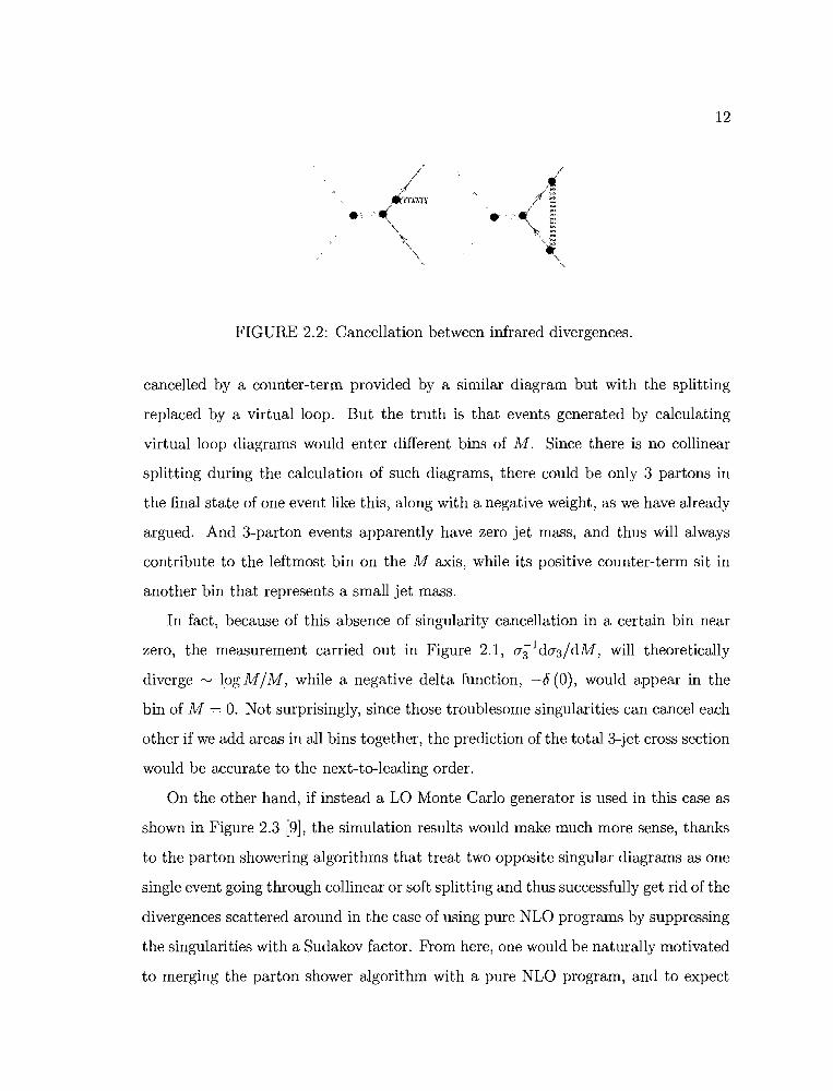
12
FIGURE 2.2: Cancellation between infrared divergences.
cancelled by a counter-term provided by a similar diagram but with the splitting
replaced by a virtual loop. But the truth is that events generated by calculating
virtual loop diagrams would enter different bins of M. Since there is no collinear
splitting during the calculation of such diagrams, there could be only 3 partons in
the final state of one event like this, along with a negative weight, as we have already
argued. And 3-parton events apparently have zero jet mass, and thus will always
contribute to the leftmost bin on the M axis, while its positive counter-term sit in
another bin that represents a small jet mass.
In fact, because of this absence of singularity cancellation in a certain bin near
zero, the measurement carried out in Figure 2.1, lJ3"ldlJ3/dM, will theoretically
diverge rv logM/M, while a negative delta function, -£5(0), would appear in the
bin of M = O. Not surprisingly, since those troublesome singularities can cancel each
other if we add areas in all bins together, the prediction of the total 3-jet cross section
would be accurate to the next-to-leading order.
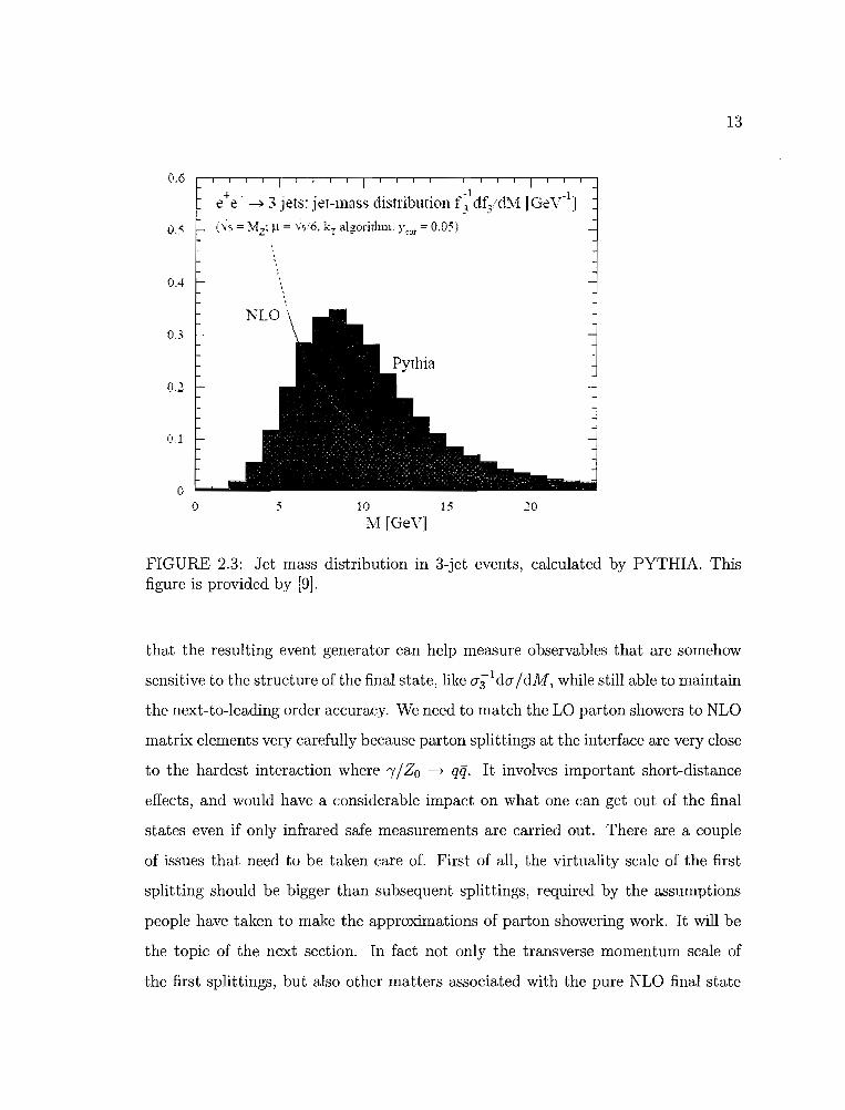
On the other hand, if instead a LO Monte Carlo generator is used in this case as
shown in Figure 2.3 [9], the simulation results would make much more sense, thanks
to the parton showering algorithms that treat two opposite singular diagrams as one
single event going through collinear or soft splitting and thus successfully get rid of the
divergences scattered around in the case of using pure NLO programs by suppressing
the singularities with a Sudakov factor. From here, one would be naturally motivated
to merging the parton shower algorithm with a pure NLO program, and to expect
13
0.6
e+e- --4 3 jets: jet-mass distribution f;\lt~/(l:VllGeylJ
0.5 t'is = YIz: ~l = '-",6. kr algorirhm. Y.;", = 0.05)
0.4
0,3
02
0.1
oo 10 15
:v11GeVI20
FIGURE 2.3: Jet mass distribution in 3-jet events, calculated by PYTHIA. Thisfigure is provided by [9].
that the resulting event generator can help measure observables that are somehow
sensitive to the structure of the final state, like a31da/ dM, while still able to maintain
the next-to-leading order accuracy. We need to match the LO parton showers to NLO
matrix elements very carefully because parton splittings at the interface are very close
to the hardest interaction where t/Zo ~ qq. It involves important short-distance
effects, and would have a considerable impact on what one can get out of the final
states even if only infrared safe measurements are carried out. There are a couple
of issues that need to be taken care of. First of all, the virtuality scale of the first
splitting should be bigger than subsequent splittings, required by the assumptions
people have taken to make the approximations of parton showering work. It will be
the topic of the next section. In fact not only the transverse momentum scale of
the first splittings, but also other matters associated with the pure NLO final state
14
partons like flavor, color, etc., should also be translated carefully to the language of
parton showering. Secondly, when the LO diagrams are combined with the first stage
of showering and one also includes pure NLO graphs, some short-distance effects that
used to be calculated by hard NLO matrix elements have now also been included in
some of the first splittings. So efforts must be made to avoid possible double counting
as well.
2.4 Parton Evolution
2.4.1 Introduction
Today perturbative calculations in QCD have only been performed to next-to
leading order in most cases. The computation involved if we go to higher fixed order
would approximately increase factorially, and this probably cannot be solved anytime
soon. Meanwhile the effects of a portion of all higher order terms could be enhanced
in certain region of the phase space, and need to be taken into account if one wants
to avoid unphysical divergences and get sensible theoretical predictions throughout
the entire kinematic region of final-state particles. So instead of calculating endless
higher order Feynman graphs accurately, an algorithm called "parton showering" has
been developed to sum over certain kinds of terms approximately to all orders in the
phase space region where they become important. This algorithm usually deals with
interactions with a virtuality scale t > to, and to is a infrared cut-off scale which
are usually taken to be of order 1 GeV. Beyond this cut-off scale non-perturbative
effects would get more important and thus can not be neglected anymore. Often
people would use a phenomenological hadronization model to take over from here.
Those two algorithms together could then coexist perfectly together in a numerical
program, known as Monte Carlo event generator.
In this section, brief calculations will be given to illustrate what a typical
showering algorithm is, starting with introducing parton splitting functions in the
15
b
a &;)
... 6 c
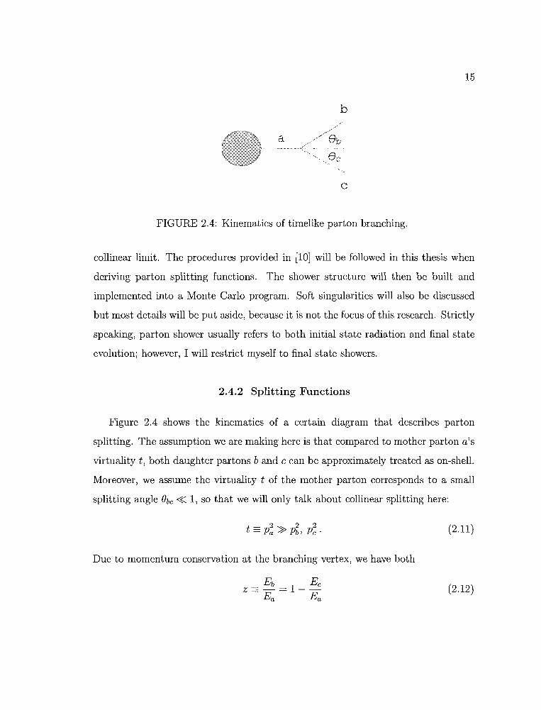
FIGURE 2.4: Kinematics of timelike parton branching.
collinear limit. The procedures provided in [10] will be followed in this thesis when
deriving parton splitting functions. The shower structure will then be built and
implemented into a Monte Carlo program. Soft singularities will also be discussed
but most details will be put aside, because it is not the focus of this research. Strictly
speaking, parton shower usually refers to both initial state radiation and final state
evolution; however, I will restrict myself to final state showers.
2.4.2 Splitting Functions
Figure 2.4 shows the kinematics of a certain diagram that describes parton
splitting. The assumption we are making here is that compared to mother parton a's
virtuality t, both daughter partons band c can be approximately treated as on-shell.
Moreover, we assume the virtuality t of the mother parton corresponds to a small
splitting angle Obc « 1, so that we will only talk about collinear splitting here:
t - 2"" 2 2= Pa // Pb, Pc .
Due to momentum conservation at the branching vertex, we have both
(2.11)
(2.12)
----------- - ------- -
16
and
= 2EbEc(1 - cos ebc )
~ EbEce~
= z (1 - z) E~e~c (2.13)
z is known as the energy fraction. In the last equation, small angel approximation
has been applied thanks to the fact that parton a is only slightly off-shell. It is
not hard to see that t is always positive if Eq.(2.11) is satisfied, and such a process
is given the name 'time-like branching'. Before proceeding, the relations between
different angels in the splitting also need to be worked out. In the plane defined by
this splitting, applying momentum conservation, together with the small angle and
on-shell approximation 1P1 ~ E for parton band c, the following can be derived:
As a result,
ebC=~~=~=ecEaY~ 1-z z'
(2.14)
(2.15)
Now let us start calculating some specific time-like branching diagrams. To start
with, let all three partons a,b,c be gluons. According to the Feynman rule for the
triple-gluon vertex,
(2.16)
where 0', (3, "I are Dirac indices; A, B, C are indices of SU(3) gauge group's generators;
a, b, C are parton indices; E:f is the polarization vector for gluon i; fABC is the structure
constant of the Lie algebra of the gauge group. In addition, all three momenta will
be defined as outgoing, and that leads to -Pa = Pb + Pc. Now that all three gluons
are almost on shell, considering the Ward Identity for non-Abelian gauge theories,
17
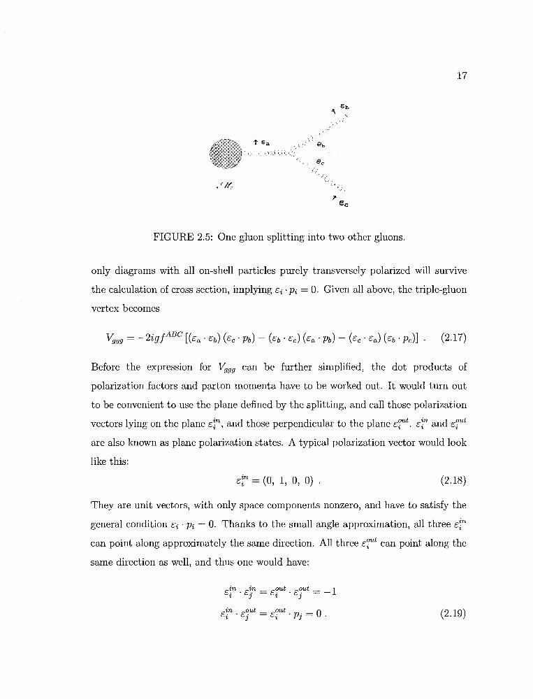
61"
FIGURE 2.5: One gluon splitting into two other gluons.
only diagrams with all on-shell particles purely transversely polarized will survive
the calculation of cross section, implying Ei . Pi = O. Given all above, the triple-gluon
vertex becomes
(2.17)
Before the expression for ~gg can be further simplified, the dot products of
polarization factors and parton momenta have to be worked out. It would turn out
to be convenient to use the plane defined by the splitting, and call those polarization
vectors lying on the plane E~n, and those perpendicular to the plane Eft. E~n and Efut
are also known as plane polarization states. A typical polarization vector would look
like this:
E~n = (0, 1, 0, 0) . (2.18)
They are unit vectors, with only space components nonzero, and have to satisfy the
general condition Ei . Pi = o. Thanks to the small angle approximation, all three E1n
can point along approximately the same direction. All three Eft can point along the
same direction as well, and thus one would have:
(2.19)
18
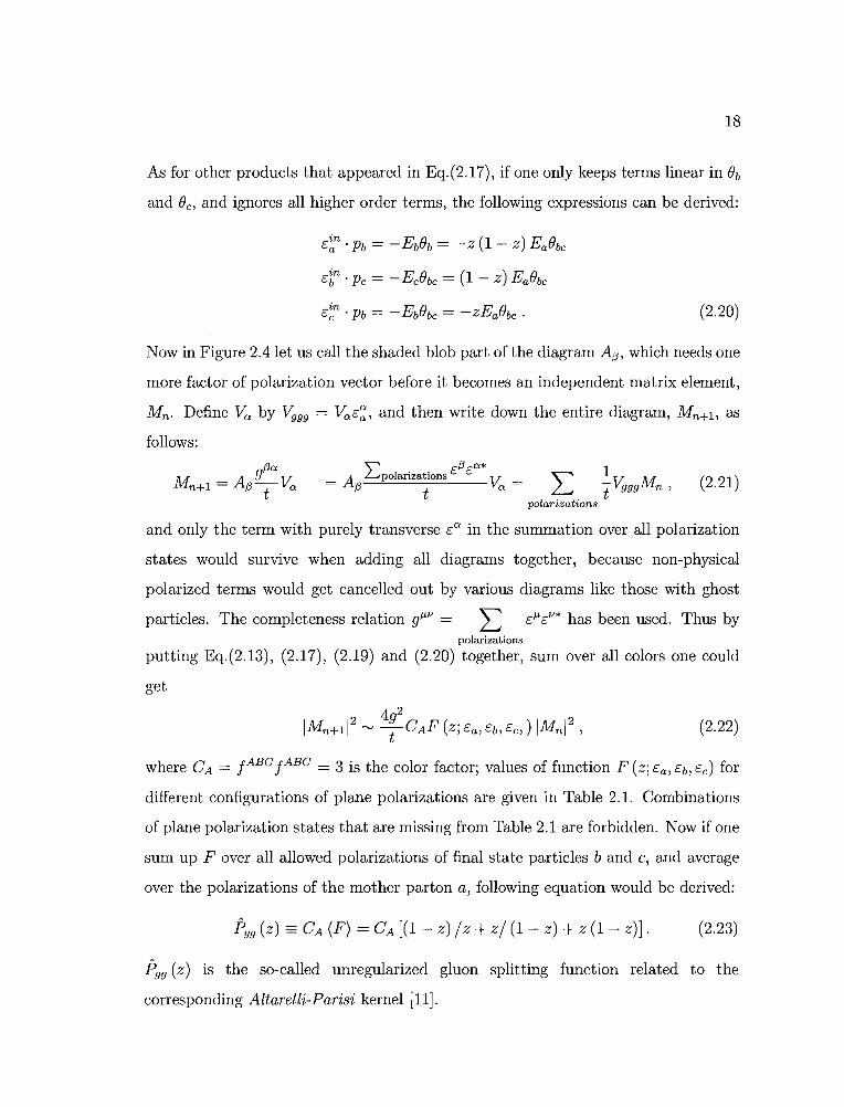
As for other products that appeared in Eq.(2.17), if one only keeps terms linear in (h
and ()e, and ignores all higher order terms, the following expressions can be derived:
E~n . Pb = -Eb()b = -z (1 - z) Ea()be
E~n • Pc = - Ee()be = (1 - z) Ea()be
(2.20)
Now in Figure 2.4 let us call the shaded blob part of the diagram A.a, which needs one
more factor of polarization vector before it becomes an independent matrix element,
Mn . Define Va by ~gg = VaE~, and then write down the entire diagram, Mn+1 , as
follows:
'\' .a a* 1_ A L...,polarizations E E T 7 _ '""'-.a t Va - ~ t ~ggMn ,polarizations
(2.21)
and only the term with purely transverse Ea in the summation over all polarization
states would survive when adding all diagrams together, because non-physical
polarized terms would get cancelled out by various diagrams like those with ghost
particles. The completeness relation gJ.J.1.1 = L E)J.E1.I* has been used. Thus bypolarizations
putting Eq.(2.13), (2.17), (2.19) and (2.20) together, sum over all colors one could
get
(2.22)
where CA = fABC fABC = 3 is the color factor; values of function F (z; Ea , Eb, Ee ) for
different configurations of plane polarizations are given in Table 2.1. Combinations
of plane polarization states that are missing from Table 2.1 are forbidden. Now if one
sum up F over all allowed polarizations of final state particles band c, and average
over the polarizations of the mother parton a, following equation would be derived:
(2.23)
?gg (z) is the so-called unregularized gluon splitting function related to the
corresponding Altarelli-Parisi kernel [11].

19
TABLE 2.1: Polarization dependence of collinear branching 9 ~ 99
Ca Cb Cc F (z; ca, cb, cc)in in in (1 - z) /z + z/ (1 - z) + z (1- z)in out out z (1 - z)out in out (l-z)/zout out in z/(l-z)
Before starting the discussion of other types of parton branching, it is worthwhile
to stop and dig into the current case of branching a bit more. One can easily make the
observation based on Table 2.1 that the splitting function would become divergent
when the daughter gluon polarized in the plane of branching is soft. It is then natural
to go on and ask what kind of correlation it would be between the plane of branching
and the polarization of the mother parton. Let us call the angel ¢ between parton
a's polarization vector and the plane of branching, and then
C = cos ~cin + sin ~couta 'Pa 'f/a'
therefore this time the splitting function
= cos2¢ [1 M (c~n,ctn,c~n) 12 + 1M (c~n,cr't,c~ut) \2] +
sin2¢ [1 M(c~ut,ctn,c~t) 12+ 1M (C~t,cbut,c~n) 12
]
= cos2¢ [1 - z + -11 + 2z (1 _ z)] + sin2 ¢ [1 - z + _1_]z -z z 1-z
1- z 1= -- + -1- + z (1 - z) + z (1 - z) cos 2¢ ,
z -z
(2.24)
(2.25)
(2.26)
and notice there are no cross terms as M* (c~n,cb,cc) M (c~ut,cb,cc) in the above
calculation. That is because each matrix element appearing in the above equation
includes nothing more than a single splitting vertex and is hence purely imaginary.
Any cross term will therefore be exactly cancelled out by its complex conjugate
term. Apparently, in Eq.(2.25), the first three terms in the last line give exactly the
20
b
l' x
c
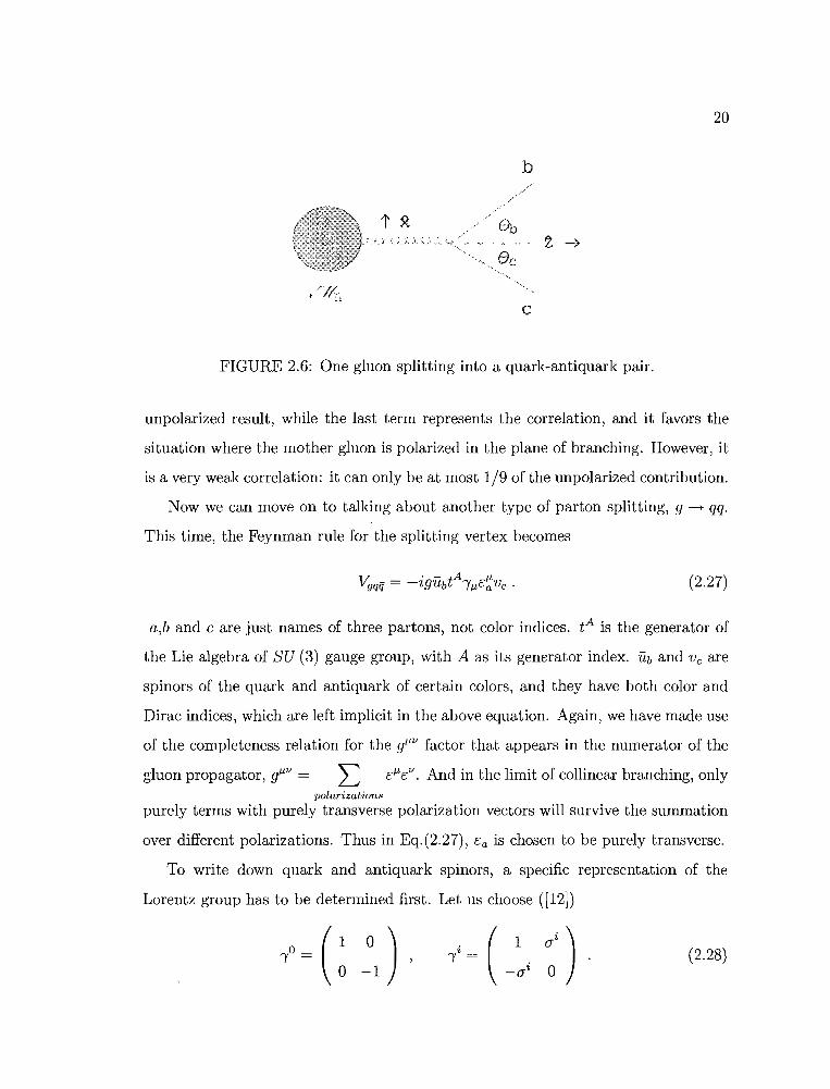
FIGURE 2.6: One gluon splitting into a quark-antiquark pair.
unpolarized result, while the last term represents the correlation, and it favors the
situation where the mother gluon is polarized in the plane of branching. However, it
is a very weak correlation: it can only be at most 1/9 of the unpolarized contribution.
Now we can move on to talking about another type of parton splitting, g ~ qq.
This time, the Feynman rule for the splitting vertex becomes
(2.27)
a,b and c are just names of three partons, not color indices. tA is the generator of
the Lie algebra of SU (3) gauge group, with A as its generator index. fh and V c are
spinors of the quark and antiquark of certain colors, and they have both color and
Dirac indices, which are left implicit in the above equation. Again, we have made use
of the completeness relation for the glLlJ factor that appears in the numerator of the
gluon propagator, gf.l-/J = r:h;/J. And in the limit of collinear branching, onlypolarizations
purely terms with purely transverse polarization vectors will survive the summation
over different polarizations. Thus in Eq.(2.27), ea is chosen to be purely transverse.
To write down quark and antiquark spinors, a specific representation of the
Lorentz group has to be determined first. Let us choose ([12])
(2.28)
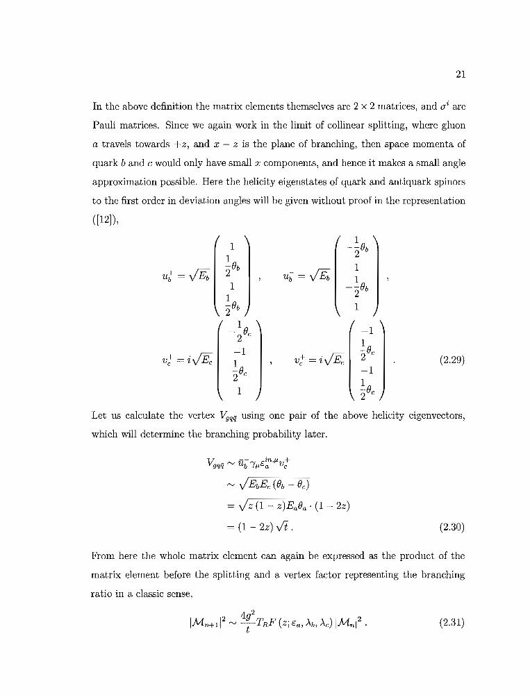
21
In the above definition the matrix elements themselves are 2 x 2 matrices, and (Ji are
Pauli matrices. Since we again work in the limit of collinear splitting, where gluon
a travels towards +z, and x - z is the plane of branching, then space momenta of
quark band c would only have small x components, and hence it makes a small angle
approximation possible. Here the helicity eigenstates of quark and antiquark spinors
to the first order in deviation angles will be given without proof in the representation
([12]),
11 --Bb
1 2-Bb
ub = VB;121
1 --Bb
1 2-Bb 12
1-1--B2 e
~B-11 v+ = iVEc 2 e (2.29)e e
2Be -11
1 2Be
Let us calculate the vertex Vgqq using one pair of the above helicity eigenvectors,
which will determine the branching probability later.
'" JEbEe(Bb - Be)
= Jz (1- z)EaBa · (1- 2z)
= (1 - 2z) Vi . (2.30)
From here the whole matrix element can again be expressed as the product of the
matrix element before the splitting and a vertex factor representing the branching
ratio in a classic sense,
(2.31)
22
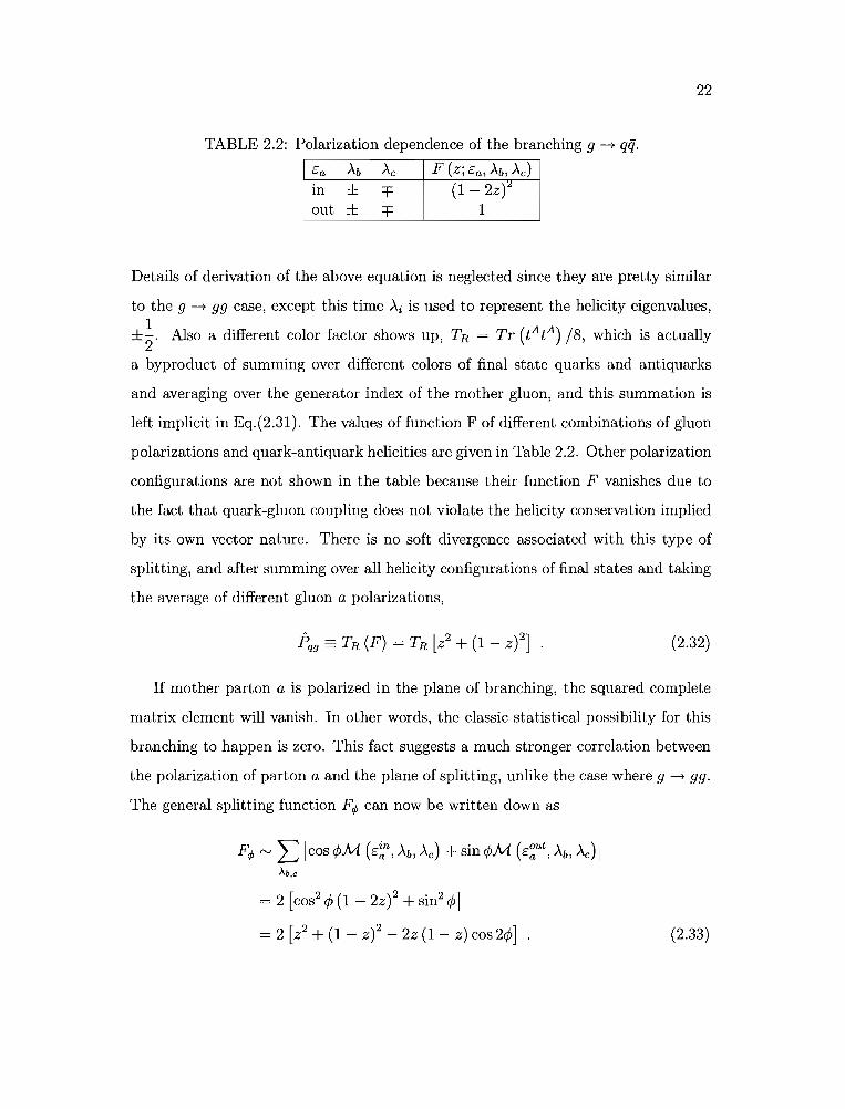
TABLE 2.2: Polarization dependence of the branching g ~ qq.
Ca Ab Ac F (z; Ca, Ab' Ac)
III ± =F (1 - 2z):4out ± =F 1
Details of derivation of the above equation is neglected since they are pretty similar
to the g ~ gg case, except this time Ai is used to represent the helicity eigenvalues,1±2"' Also a different color factor shows up, TR = Tr (tAtA) /8, which is actually
a byproduct of summing over different colors of final state quarks and antiquarIes
and averaging over the generator index of the mother gluon, and this summation is
left implicit in Eq. (2.31). The values of function F of different combinations of gluon
polarizations and quark-antiquark helicities are given in Table 2.2. Other polarization
configurations are not shown in the table because their function F vanishes due to
the fact that quark-gluon coupling does not violate the helicity conservation implied
by its own vector nature. There is no soft divergence associated with this type of
splitting, and after summing over all helicity configurations of final states and taking
the average of different gluon a polarizations,
A [ 2 2JPqg == TR (F) = TR Z + (1 - z) (2.32)
If mother parton a is polarized in the plane of branching, the squared complete
matrix element will vanish. In other words, the classic statistical possibility for this
branching to happen is zero. This fact suggests a much stronger correlation between
the polarization of parton a and the plane of splitting, unlike the case where g ~ gg.
The general splitting function F", can now be written down as
F", rv L Icos¢M (c~n, Ab' Ac) + sin¢M (c~t, Ab' Ac) IAb,c
= 2 [cos2 ¢ (1 - 2Z)2 + sin2 ¢J
= 2 [Z2 + (1 - Z)2 - 2z (1 - z) cos 2¢J (2.33)
23
b
Ec
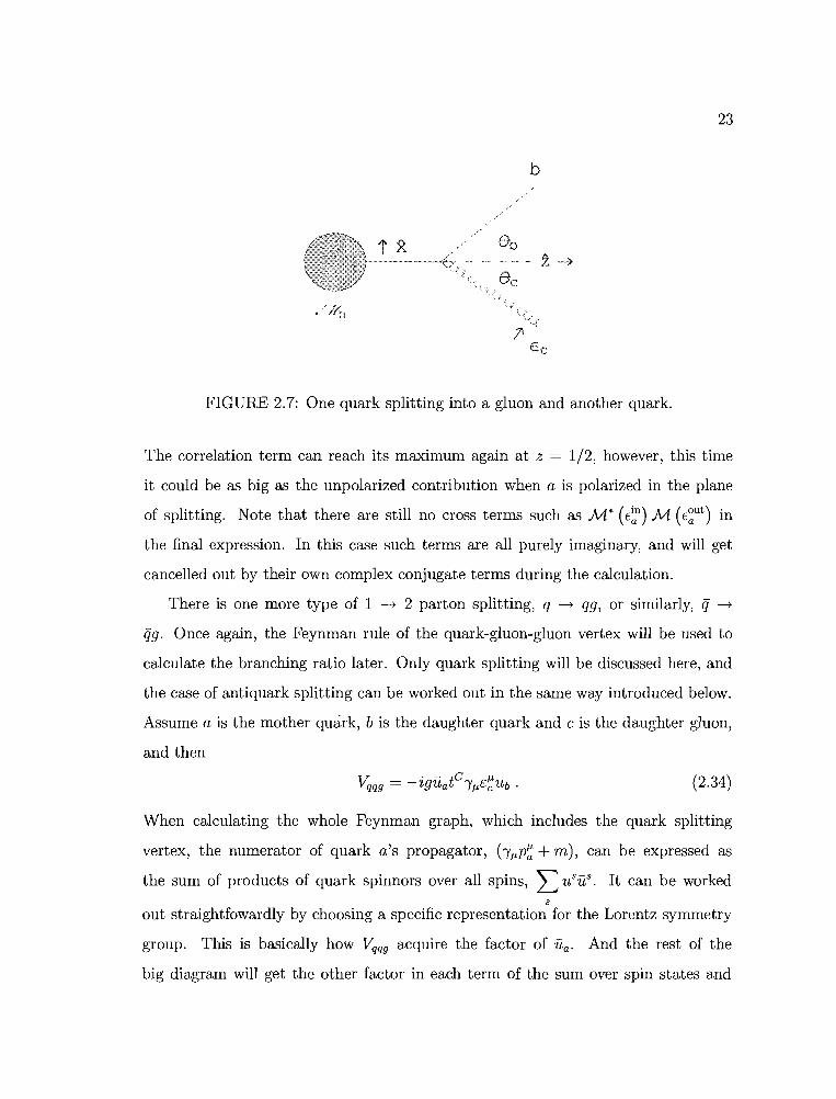
FIGURE 2.7: One quark splitting into a gluon and another quark.
The correlation term can reach its maximum again at z = 1/2, however, this time
it could be as big as the unpolarized contribution when a is polarized in the plane
of splitting. Note that there are still no cross terms such as M* (E::') M (E~ut) in
the final expression. In this case such terms are all purely imaginary, and will get
cancelled out by their own complex conjugate terms during the calculation.
There is one more type of 1 -> 2 parton splitting, q -> qg, or similarly, ij ->
ijg. Once again, the Feynman rule of the quark-gluon-gluon vertex will be used to
calculate the branching ratio later. Only quark splitting will be discussed here, and
the case of antiquark splitting can be worked out in the same way introduced below.
Assume a is the mother quark, b is the daughter quark and c is the daughter gluon,
and then
(2.34)
When calculating the whole Feynman graph, which includes the quark splitting
vertex, the numerator of quark a's propagator, b'LP~ + m), can be expressed as
the sum of products of quark spinnors over all spins, ~ usus. It can be workedS
out straightfowardly by choosing a specific representation for the Lorentz symmetry
group. This is basically how ~qg acquire the factor of ua' And the rest of the
big diagram will get the other factor in each term of the sum over spin states and
24
becomes a complete matrix element. But only when the quark virtuality is much
smaller compared to the hard scattering scale can one justify the above treatments
on quark a's propagator, because strictly speaking, only on-shell fermions can be
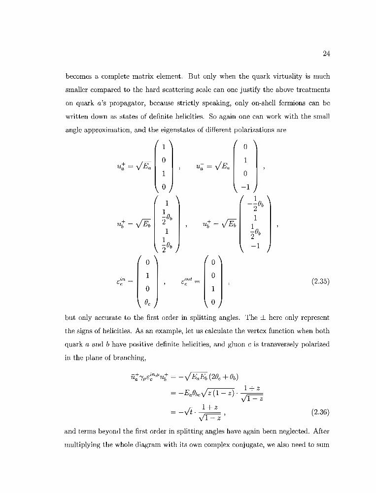
written down as states of definite helicities. So again one can work with the small
angle approximation, and the eigenstates of different polarizations are
1 0
ut = VEa 0 u;; = VEa 1
1 0
0 -1
11
--(h1 2
ut = jE;-Bb ut = jE;
121
1 -Bb
1 2-Bb -12
0 0
Ein =
1E
out =0
(2.35)e e0 1
Be 0
but only accurate to the first order in splitting angles. The ± here only represent
the signs of helicities. As an example, let us calculate the vertex function when both
quark a and b have positive definite helicities, and gluon c is transversely polarized
in the plane of branching,
(2.36)
and terms beyond the first order in splitting angles have again been neglected. After
multiplying the whole diagram with its own complex conjugate, we also need to sum
(2.37)
25
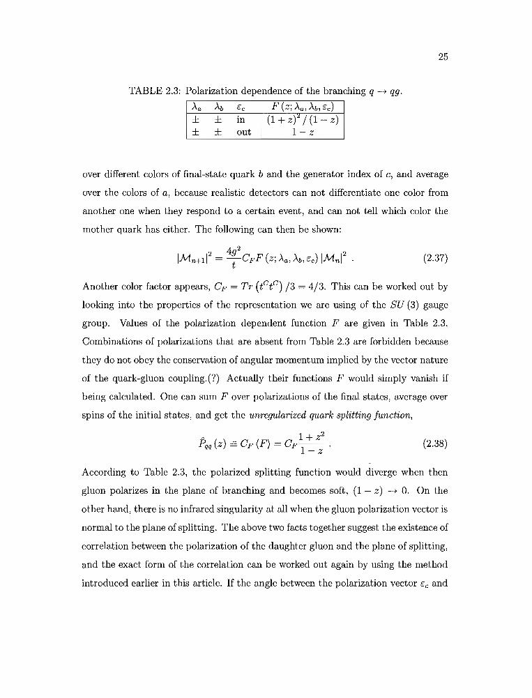
TABLE 2.3: Polarization dependence of the branching q -+ qg.
Aa Ab Ce F (z; Aa , Ab' ce)± ± in (l+zY/(l-z)± ± out 1-z
over different colors of final-state quark b and the generator index of c, and average
over the colors of a, because realistic detectors can not differentiate one color from
another one when they respond to a certain event, and can not tell which color the
mother quark has either. The following can then be shown:
2 4g22IMn+11 = -CFF (Z; Aa , Ab' ce) IMnl
t
Another color factor appears, CF = Tr (tCtC) /3 = 4/3. This can be worked out by
looking into the properties of the representation we are using of the SU (3) gauge
group. Values of the polarization dependent function F are given in Table 2.3.
Combinations of polarizations that are absent from Table 2.3 are forbidden because
they do not obey the conservation of angular momentum implied by the vector nature
of the quark-gluon coupling.(?) Actually their functions F would simply vanish if
being calculated. One can sum F over polarizations of the final states, average over
spins of the initial states, and get the unregularized quark splitting junction,
A 1 + Z2Pqq (z) == CF (F) = CF-- .
1-z(2.38)
According to Table 2.3, the polarized splitting function would diverge when then
gluon polarizes in the plane of branching and becomes soft, (1 - z) -+ O. On the
other hand, there is no infrared singularity at all when the gluon polarization vector is
normal to the plane of splitting. The above two facts together suggest the existence of
correlation between the polarization of the daughter gluon and the plane of splitting,
and the exact form of the correlation can be worked out again by using the method
introduced earlier in this article. If the angle between the polarization vector Ce and
26
the plane of branching is defined to be ¢, then
F<p r-.J ~ L [cos ¢M (z; Au, Ab, c~n) + sin ¢M (z; Au, Ab' c~ut) 12
Aa,b
(1 + )2=cos2¢ Z +sin2¢(1-z)
1-z1 + Z2 2z
= -- + -- cos2¢.1-z 1-z
(2.39)
In the first line of Eq.(2.39), there is a factor of 1/2 in front of the sum over spins
of both quarks because a is not in the final state, and therefore one should take the
average over its spin states. Similar to what have been shown in the first two types
of parton splitting, the first term represents the unpolarized splitting, and the second
term is the correlation.
Up until now, having discussed the gluon polarization angle correlation of all
three types of parton branching, one can come to several conclusions. In the collision
process of e+e- --7 qq, when a gluon is emitted from one of the very first two quarks,
it would tend to be polarized in the plane of splitting. When this gluon itself splits
again, the plane of branching is more likely to be perpendicular to the mother gluon's
polarization factor. The hardest two jets in the realistic final state of this process
usually follow the directions of the two quarks out of the primary interaction vertex,
while the softest two jets follow the directions of the produced quarks or gluons.
If we temporarily put aside the triple gluon vertex, and assume QCD is described
by an Abelian gauge theory, and then measure the angle between the plane of the
hardest two jets and the plane of the softest two jets, we would be able to find out
a distribution of cross section peaked at 90D of this angle, which is named as the
Bengtsson-Zerwas angle. But the truth is, the maximum of this distribution appear
around the Bengtsson-Zerwas angle being 60D, and the curve of distribution is much
flatter than what an Abelian gauge theory would predict it to be. The experiment
of measuring Bengtsson-Zerwas has certainly ruled out the possibility of QCD being
constructed as an Abelian gauge thoery. But if putting the triple gluon vertex back

27
in, as required by the non-Abelian, SU (3) gauge theory, and taking into account the
fact that 9 -t 99 is dominant in QCD, one could give a theoretical prediction which
match the experimental data of measuring the Bengtsson-Zerwas angle extremely
well.
It is worthwhile to determine the relation between the differential cross section of
a certain QCD process, (J"n, and the differential cross section of the same process with
one final state parton going slightly off-shell and splitting into two more partons,
(J"n+!' To begin with, the cross section without the splitting is expressed as
(2.40)
where F is the initial-state flux, same for both (J"n and (J"n+l, and d<I>n is the group of
final-state phase space integration variables,
d3~
Pa d3~
Pn (2.41)
Assume now parton a splits into two other partons band c, then the integration
variables would become
d3~
Pn (2.42)
Apply the energy and momentum conservation, fla = ilb + Pc and Ea = Eb + Ee , one
can multiply several identity integrals with d<I>n+! in the small angle approximation,
which are listed below:
1 = J8 (p-:, - ilb - flc) d3fla ,
1 = J8 (z - ;:) dz . (2.43)
The last two integrals are suggested by the kinematics we have been using through
out the derivation of various parton splitting functions. Consequently the integration
variable d3flc in <I>n+l can be replaced by d3fla by carry out the integral of d3flc, and
28
the factor of energy E c in the denominator can also be replaced by Ea (1 - z). By
doing the above operations d<Pn+l can be transformed to
(2.44)
The third line of the last equation is derived by carrying out the integral over dEb
and d(h. And note that d3pb = E~ObdEbd(hd¢ is only true when Ob « 1. Now we are
fully equipped to write down
do-n+1 = F IMn+1 12
d<Pn+l
4g2 1= F-CF IMn l
2 d<P n 3dtdzd¢t 4 (21T)
= do-ndt dz d¢ asCF .t 21T 21T
(2.45)
C and F here are the corresponding color factor and polarized z-distribution function,
and the strong coupling constant as = i / (41T). One can integrate out the azimuthal
angle ¢ to further simplify this equation:
Jd¢ A
21T CF = Pba (z) , (2.46)
(2.47)
and ?ba (z) is the splitting function of the studied branching process, and hence one
can write downdt as A
dO-n+1 = do-n-dz-Pba (z) .t 21T
Discussion about space-like branching will be omitted here, since it is only related to
Initial-State Radiation(ISR), which is not the concern of this thesis.
29
2.4.3 Parton Evolution
Processes like e+e- --> hadrons typically have many particles in the final states,
and apparently a big number of hadrons cannot be evolved directly from just 3 or
4 partons produced by the hardest interaction. Some important intermediate steps
have to be studied before one can even start to talk about the stage of hadronization.
Especially if one wants to build a Monte Carlo event generator that can both be
accurate to the next-to-Ieading order and give physical final-state particles, one would
have to figure out an approach to make many more partons out of the very few quarks
and gluons that can be produced by a pure NLO program, so that the hadronization
model can be started with a large enough number of partons. Unfortunately, when
summing over all necessary Feynman graphs that can give rise to many final state
partons, it is very difficult to take virtual graphs into account properly. However,
one can make use of the splitting functions that have been just introduced to make
up a model where very few partons could repeatedly split into more partons, with
branching ratios given by classical statistics.
To begin with, let us study a simplified model suggested in [13] where only one
type of massless scalar particles can be produced by the e+e- collision and only this
same kind of particles would be involved in the formation of hadrons that can be
finally detected by lab equipments. Many details of interactions among those scalar
particles are not the major concerns here either, but collinear divergences similar to
those in QCD process can still be present if one specifies the properties of the scalar
particles in a certain way, for example, it can have an interaction term of q}, and
lives in a space with six dimensions. Anyway, the cross section to measure a certain
infrared-safe observable F can still be written down as
a[F] = L~!J[d{P}ml 1M ({P}m)12
F({P}m) ,m
(2.48)
30
and the integrations are defined as
(2.49)
which can put all final state momenta on shell with the factors 0" (pD, and force the
momentum being conserved throughout the collision, with Po = (-IS, 0). M ({p}m)
as before is the matrix element to produce m partons with momentum configuration
{p}m' and F ({p}m) gives the value of the measurement of such a set of partons.
Now since people have big trouble calculating all those matrix elements, we will
use a function p ({p}nJ to stand for an approximated cross section of having m
partons in the final state, and use it to replace the factor of squared matrix element
in Eq.(2.48). The function p will be derived by using small angle approximation
on particles with small virtualities splitting into two collinear particles. Basically,
the cross sections of all processes with more than two or three final-state particles
will be calculated by multiplying M ({p}n=2 or 3) with the classical total probability
of branching the first n particles to m particles in the end. Since the branching
probabilities that have been discussed earlier have no explicit time dependence, then
time would not be a good variable to control the particle evolution process. However,
those probabilities depend on the virtualities of the involved splitting, and thus one
can invent another variable t that is directly related to the virtuality to play to role
of 'time'. For now we want this new variable t to have the property that at the
beginning of the evolution, which is also the product of the hardest interaction, t is
equal to zero; and the particles would stop splitting when t reaches a certain cutoff
value tf. To satisfy the above conditions, in QeD, one can define
q2t == log ~ , (2.50)
q
where q6 describes the virtualities of the hardest quarks and gluons given by the hard
matrix elements, and q2 is the virtuality of the current splitting. This way, at the
beginning of the evolution, the 'shower time' is tuned to be zero; and as the time
like branchings move on, the virtuality scales would drop, while the corresponding
(2.51)
31
"shower time" would increase until it hits the cutoff value. But for the purpose of
the discussion here where the interaction only involves one type of massless scalar
particles, there is another way to define the variable t. In the splitting l -> i + j we
can chooseQ2
t == log 02Pi . Pj
where Q~ is the virtuality scale at which the shower starts.
Now if at a certain stage of 'shower time' t of the parton evolution we write down
the cross section of having m particles with momenta {p} m as P ({p}m , t), then the
total cross section of present 'shower time' can be expressed in terms of function p,
aT (t) = L ~! J[d {p}m] p ({p}m' t) .m
(2.52)
More generally, if the measurement function is not just equal to 1, at the cutoff
"shower time" t j, one would instead have
a[F] = L ~! J[d{P}m]P({P}m,tj)F({P}m)m
(2.53)
Before we proceed, it will be helpful to set up a formalism (adapted from [13]) now
for the discussion later. Define a certain vector space of functions, where a certain
state IG (t)) (or (G (t)l) corresponds to a group of functions at a chosen t, which
describes the same property of an event regardless of its momentum configuration.
For example, (FI corresponds to the collection of functions F ({p}m) (we drop the
argument t because measurement functions are generally independent of t), and the
state IP (t)) corresponds to the collection of cross sections P ({p} m , t) at a certain
"shower time" t. Furthermore, the inner product of the vector space can be defined
to be
(AlB) == L ~! J[d{P}m] A ({P}m) B ({p}m) .m
(2.54)
Define a complete set of orthogonal basis vectors I{p}n) such that they would have
the following property:
(2.55)
32
with the completeness relation
1 = L ~! J[d{P}ml I{P}m) ({P}mlm
(2.56)
Obviously, any measurement function F can correspond to a vector (FI, and thus
the cross section of the observable at the final stage would be
(2.57)
There is a special state which corresponds to a function that gives all final state the
same value, 1, and let us name that state (11 whose inner product with the state
IP (t)) gives us the total cross section at a certain stage
(JT = (lip (t)) . (2.58)
A non-trivial example of (FI is (N) 51, and it corresponds to any function that
returns 1 for events with more than 5 final state particles and returns 0 otherwise.
Therefore,
(IN>5 = (N > 51p (t)) (2.59)
would be the cross section of having at least 5 partons in the final state at t.
By now, the problem of figuring out how the final state partons evolve has become
the task of studying the 'shower time' evolution operator that acts on the state [p (t)).
Typically one would start with a defined number of particles. For example, if we pick
an initial state Ip (0)) such that the event has only 2 particles at t = 0, then we would
have ({p}2Ip (0)) =F 0 but ({P}m Ip (0)) = 0 for any m > 2. Obviously, ({p}2Ip (0))
is the Born level cross section. After evolving this state to the cut-off scale tt, we
would obtain the final state Ip (tt)), which we can use to calculate the final-state
cross section at that scale.
Define the evolution operator to be U (t, t'), and
Ip(t)) =U(t,t') Ip(t')) (2.60)
33
It could also have the group composition property,
(2.61)
Intuitively thinking, if such operator acts on a certain state, the effects should be
either some particles in that state split into more particles, or nothing happens at all.
Then a reasonable guess would be the evolution operator consists of two parts, one
would leave the state untouched with a certain probability, and another make the
state become another state by making particles fragment, also with some probability.
Let us look at the latter part first. For this purpose, an infinitesimal generator of
evolution, 1i (t), is needed. At the lowest order, when it acts on an arbitrary state,
1i (t) Ip (t)), it makes one particle l in the original state split into two other particles,
with momenta PI and Pm+l respectively. In this model involving only one type of
massless scalar particles, the matrix element after the splitting is
(2.62)
where 9 is the coupling constant of the interaction. But in order to make the above
equation approximately right, one condition has to be satisfied that the splitting
happens in the collinear limit, because only when the splitting is nearly collinear can
one find a momentum PI ~ PI + im+1 while nevertheless on shell, pf = 0, which would
not change the momentum configuration in the smaller diagram much. In fact the
approximated factorization of the bigger diagram M m +1 is the key to developing an
algorithm of parton showers. For a statistical splitting function, one needs to square
the quantum amplitudes above. For QeD, the splitting function at a certain scale
of hardness or virtuality has already been worked out in the previous sections. The
projection of the state Ip (t)) on to the basis vector I{P}m+l) after the operation of
the Hamiltonian 1i (t), or in other words, the cross section p ({p}m+l ,t) of the final
state, is now approximately a sum of the cross sections of m final state particles

•••
-I
i{
I,-I :I -ir
~J-j-
+•••
34
(2.63)
FIGURE 2.8: Illustration of the effects of evolution operator. This figure is providedby [13].
multiplied by probabilities for different particles to split:
({P}m+111i(t)lp)~L8(t-Iog2~Q~ ) (2~ g~ )2 ({P}mIP)t Pt . Pm+l Pt . Pm+l
The 8 function has been inserted which shows the evolution is at 'shower time' t.
And now the choice of t here in this model seems quite natural based on the form of
the statistical splitting function.
The other part of the evolution operator U (t' ,t) that leaves the particle number
and momentum configuration of any state unchanged can be written as N (t' ,t). It
should also have the group composition property
(2.64)
Other than that, when it acts on the basis vectors, the resulting states are still the
same basis vectors, but could have a new multiplicative constant, or one could say,
the basis vectors are in fact this no-change operator's eigenvectors,
(2.65)
The physical meaning of the eigenvalue will be given later.
It is time to write down the complete form of the statistical evolution operator,
(2.66)
35
which can be interpret.ed in the following way, as briefly mentioned earlier: when the
evolution operator U acts on a statistical state, it will either evolve the state without
any splitting during the entire period of 'shower time' from i l -----* i 3 , or evolve it
without splitting for a while, and at some point i 2 make some particle in the state
split, and then after the splitting evolve it normally with or without splitting to i 3 .
However, neither the probability of an arbitrary state evolving without any splitting
nor the probability of the state splitting at least once during the evolution is clear in
the above equation.
To find out about the probabilities of different ways of evolution, one can st.udy
the quantity (11 U (ii, i) Ip (i)), the total cross section after the parton evolution. A
sensible convention would be the one in which the total cross section of any studied
process remain the same throughout the evolution, thus
(}T = (lip (i)) = (11 U (ii, i) Ip (i)) , (2.67)
and since the above relation is true for any state Ip), the only possibility is the
evolution operator always has the property that
(11 U (ii, i) == (11 (2.68)
As a result, if one multiply the state Ip (i l )) to the right and (11 to the left on both
sides of the Eq.(2.66),
,~
(}T(i3) = L~!J[d{P}ml [~(i3,il;{P}m)P({P}m,il)]+m
+~ ~! J[d {P}ml [.i~t3 di2 (liH (t2 ) \{P}m) ~ (i 2 , t1 ; {P}m) p ({P}m' i 1)] ,
(2.69)
36
and based upon the last equation from a classic statistical point of view, one should
interpret (111i (t) I{p}m) as the total probability for one of the particles in state {p}m
splitting at 'shower time' t. And ~ (t', t; {p}m) should be explained as the probability
for the state to evolve from t -+ t' without splitting at all, known as the Sudakov
factor. By using the fact that total cross section does not change as the state of
partons develop, one can equate Eq. (2.69) to the expression for total cross section
defined in Eq. (2.52) at time t 1 in terms of P({P}m,td, and get
(2.70)
By taking the derivative of the last equation with respect to t 3 , one could get
(2.71)
and solving this equation gives us
(2.72)
Now come back to Eq. (2.69) again. Until now, one might still think at a given
hardness scale, the probability of one particle splitting in the state I{p}m) is
(l11i (t) I{p}m)' the counterpart of which in LO QeD calculation is the sum of
splitting functions Fgg , Fqg and Fgq over all particles that could split in the same state.
However, Eq. (2.69) implies the actual probability of splitting is in fact the Sudakov
exponential factor times the appropriate splitting function. Strictly speaking,
(2.73)
Many parton splitting functions are singular when the branching is collinear, and
it seems to endanger the whole picture of parton fragmentation. But the Sudakov
exponential could successfully suppress parton splitting in the infrared region, and
hence solves the potential problem of unphysical singular behavior.

37
2.4.4 Implementation
Having introduced the formulation of parton evolution, one can start asking
the question of how to write a computer program to simulate the parton splitting
process. Here we will first talk about the general idea of a branching algorithm, and
then elaborate on some much more sophisticated methods that have been used by
BEOWULF [14].
2.4.4.1 Generating Splitting Info Based on Given Distributions
Given the intial conditions including the hardness scales and momentum fractions
of the first few partons, the first step is to make use of the Sudakov exponential to
get the right hardness scale of the next possible branching [10]. As we already know,
L\ (t2 , td tells about the probability of a parton not to split between the two hardness
scales t 1 and t 2 , and is always a number between 0 and 1. If we get the shower time
t 1 for the initial parton by translating from the hardness scale, and want to find
out what value t 2 should take, we could let the program to generate a uniformly
distributed random number R E (0,1), and then solve the equation below for t 2 :
(2.74)
The resulting t 2 can be translated back to a hardness scale where the next splitting
will be taking place. But would t 2 have the correct distribution in that way? Take
an arbitrary R, and assume t 2 (R) is the solution to Eq (2.74). Apparently the
probability p (R) of generating a random number smaller than R would just be R
itself, and hence the probability for the solution t2 to be bigger than t2 (R) will also
be R. In other words, the probability for the algorithm not to split a parton between
t 1 and t2 (R) is exactly L\ (t2 (R) ,t1), just as what Sudakov exponential is defined to
represent.
Once we have acquired the hardness scale of the next branching, we still have to
generate the momentum fraction x of the daughter partons with respect to the mother
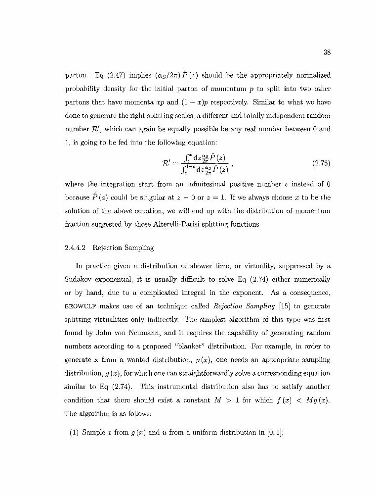
(2.75)
38
parton. Eq (2.47) implies (as/2;r) P (z) should be the appropriately normalized
probability density for the initial parton of momentum p to split into two other
partons that have momenta xp and (1 - x)p respectively. Similar to what we have
done to generate the right splitting scales, a different and totally independent random
number R', which can again be equally possible be any real number between 0 and
1, is going to be fed into the following equation:
J.X dz as P(z)R' = f 211"f-fdz~~P(z) ,
where the integration start from an infinitesimal positive number E instead of 0
because P(z) could be singular at z = 0 or z = 1. If we always choose x to be the
solution of the above equation, we will end up with the distribution of momentum
fraction suggested by those Alterelli-Parisi splitting functions.
2.4.4.2 Rejection Sampling
In practice given a distribution of shower time, or virtuality, suppressed by a
Sudakov exponential, it is usually difficult to solve Eq (2.74) either numerically
or by hand, due to a complicated integral in the exponent. As a consequence,
BEOWULF makes use of an technique called Rejection Sampling [15} to generate
splitting virtualities only indirectly. The simplest algorithm of this type was first
found by John von Neumann, and it requires the capability of generating random
numbers according to a proposed "blanket" distribution. For example, in order to
generate x from a wanted distribution, p (x), one needs an appropriate sampling
distribution, 9 (x), for which one can straightforwardly solve a corresponding equation
similar to Eq (2.74). This instrumental distribution also has to satisfy another
condition that there should exist a constant lYI > 1 for which f (x) < Mg (x).
The algorithm is as follows:
(1) Sample x from 9 (x) and u from a uniform distribution in [0,1];
39
(2) See if u < f (x) /Mg (x) is true:
a) If true, accept x as a successfully sampled point;
b) If false, reject x and repeat the algorithm from step (1).
Random points selected by the above algorithm will have the right distribution f (x),
and this can be proved using a graphical argument called the envelope principle. It
says when points are sampled from 9 (x), they can fill the area under the curve M 9 (x).
By accepting and rejecting points according to the inequality u < f (x) /Mg (x), the
selected points should be able to uniformly occupy a sub-area which is right under
the curve f (x), or in other words, those points have been sampled according to the
distribution f (x).
In BEOWULF, a more complicated version of Rejection Sampling is used when
generating the virtualities of splittings, which will be discussed later, together with a
technique to produce the splitting angle and momentum fractions of daughter partons
without solving the awkward Eq (2.75).
40
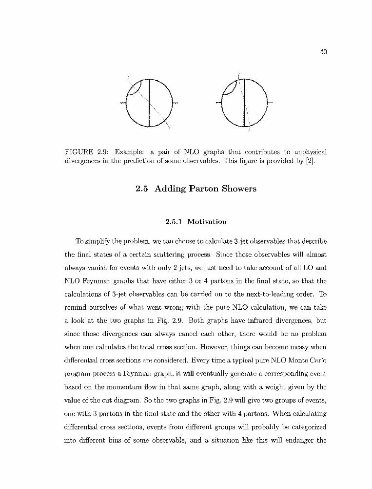
FIGURE 2.9: Example: a pair of NLO graphs that contributes to unphysicaldivergences in the prediction of some observables. This figure is provided by [2].
2.5 Adding Parton Showers
2.5.1 Motivation
To simplify the problem, we can choose to calculate 3-jet observables that describe
the final states of a certain scattering process. Since those observables will almost
always vanish for events with only 2 jets, we just need to take account of all LO and
NLO Feynman graphs that have either 3 or 4 partons in the final state, so that the
calculations of 3-jet observables can be carried on to the next-to-leading order. To
remind ourselves of what went wrong with the pure NLO calculation, we can take
a look at the two graphs in Fig. 2.9. Both graphs have infrared divergences, but
since those divergences can always cancel each other, there would be no problem
when one calculates the total cross section. However, things can become messy when
differential cross sections are considered. Every time a typical pure NLO Monte Carlo
program process a Feynman graph, it will eventually generate a corresponding event
based on the momentum flow in that same graph, along with a weight given by the
value of the cut diagram. So the two graphs in Fig. 2.9 will give two groups of events,
one with 3 partons in the final state and the other with 4 partons. When calculating
differential cross sections, events from different groups will probably be categorized
into different bins of some observable, and a situation like this will endanger the

41
/
loriFIGURE 2.10: Three types of cut propagators in the case of a quark splitting intoanother quark and a gluon. This figure is provided by [2].
cancellation of infrared divergences between events from different groups, which will
manifest itself as the weights of events.
The detailed analysis provided in the last paragraph also suggest a way of solving
the problem [2]. If we can somehow generate a single event with the effects of
both graphs in Fig. 2.9 included in a single weight accompanying this event, the
cancellation of infrared divergences would be able to work properly even if we are
dealing with differential cross sections. Any detail of the solution will depend on the
calculation of those Feynman diagrams we are interested, so it is worthwhile to take
a look at which part of those graphs are responsible for the infrared divergences and
how exactly the cancellation works out. The explanation will follow the recipe given
by [2].
Fig. 2.10 displays three different types of cut propagators, and those wavy lines
near the propagators represent the remaining parts of the Feynman diagrams plus
measurement functions. We will see very soon that they are combined to describe
how a quark or anti-quark would split into another quark and a gluon. The first
diagram has the Born level cut propagator, and its amplitude can be derived by
straight forward use of Feynman rules:
(2.76)
where q is the on-shell momentum of the cut quark propagator, and Ro denotes
factors of the rest of the diagram and measurement functions.
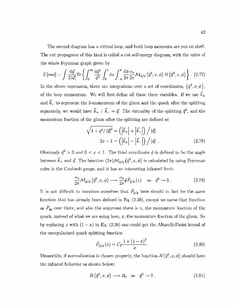
42
The second diagram has a virtual loop, and both loop momenta are put on shell.
The cut propagator of this kind is called a cut self-energy diagram, with the value of
the whole Feynman graph given by
J drY {(>O diP t 111" d1> a }I[real]= 21rJ1 Tr Jo if Jo dx _1I"21f2;Mg/q (tp,.7:,1»R(iP,x,1» . (2.77)
In the above expression, there are integrations over a set of coordinates, {iP, x, 1>},
of the loop momentum. We will first define all those three variables. If we use k+and L to represent the 3-momentum of the gluon and the quark after the splitting
separately, we would have k+ + L = if. The virtuality of the splitting iP, and the
momentum fraction of the gluon after the splitting are defined as
VI + iff 1rJ1 2= (lk+1 + ILl) /1rJ1
2x -1 = (lk+I-ILI) /1rJ1 (2.78)
Obviously iP > 0 and 0 < x < 1. The third coordinate 1> is defined to be the angle
between k+ and if. The function (21f)Mg/q (iP, x, 1» is calculated by using Feynman
rules in the Coulomb gauge, and it has an interesting infrared limit:
as ( -2 ) as A ~ ()21f Mg/q q , x, 1> ----T 21f'flPg/q x (2.79)
(2.80)
It is not difficult to convince ourselves that Pg / q here should in fact be the same
function that has already been defined in Eq. (2.38), except we name that function
as Pqq over there, and also the argument there is z, the momentum fraction of the
quark, instead of what we are using here, x, the momentum fraction of the gluon. So
by replacing z with (1 - x) in Eq. (2.38) one could get the Altarelli-Parisi kernal of
the unregularized quark splitting function
P~ () _ C 1 + (1 - X)2g/q X - F
X
Meanwhile, if normalization is chosen properly, the function R (iP, x, 1» should have
the infrared behavior as shown below:
(2.81)
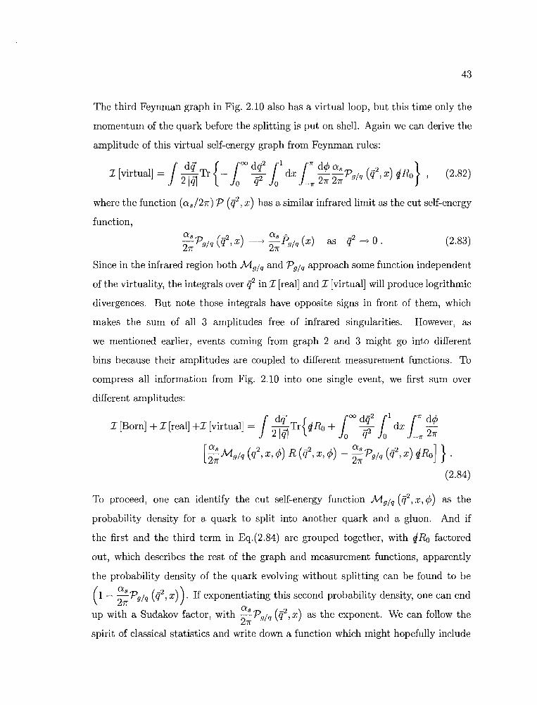
43
The third Feynman graph in Fig. 2.10 also has a virtual loop, but this time only the
momentum of the quark before the splitting is put on shell. Again we can derive the
amplitude of this virtual self-energy graph from Feynman rules:
(2.82)
where the function (Ci s /21f) P (q2, x) has a similar infrared limit as the cut self-energy
function,
Cis (-2) Cis A ()-Pgjq q , x ---+ -Pgjq X21f 21f
(2.83)
Since in the infrared region both Mgjq and Pgjq approach some function independent
of the virtuality, the integrals over q2 in I [real] and I [virtual] will produce logrithmic
divergences. But note those integrals have opposite signs in front of them, which
makes the sum of all 3 amplitudes free of infrared singularities. However, as
we mentioned earlier, events coming from graph 2 and 3 might go into different
bins because their amplitudes are coupled to different measurement functions. To
compress all information from Fig. 2.10 into one single event, we first sum over
different amplitudes:
JdrY [':>0 dq2 t j1r d¢I [Born] + I [real] +I [virtual] = 21rJ1 Tr{iRa + Jo q2 Jo dx -1r 21f
[;;Mgjq(q2,X,¢)R(q2,X,¢) - ;;Pgjq(q2,x)iRo]}.
(2.84)
To proceed, one can identify the cut self-energy function Mgjq (q2, .1:, ¢) as the
probability density for a quark to split into another quark and a gluon. And if
the first and the third term in Eq.(2.84) are grouped together, with iRa factored
out, which describes the rest of the graph and measurement functions, apparently
the probability density of the quark evolving without splitting can be found to be
( 1 - ;;Pgjq (q2, x) ). If exponentiating this second probability density, one can endCi
up with a Sudakov factor, with -!...Pgjq (q2,X) as the exponent. We can follow the21f
spirit of classical statistics and write down a function which might hopefully include
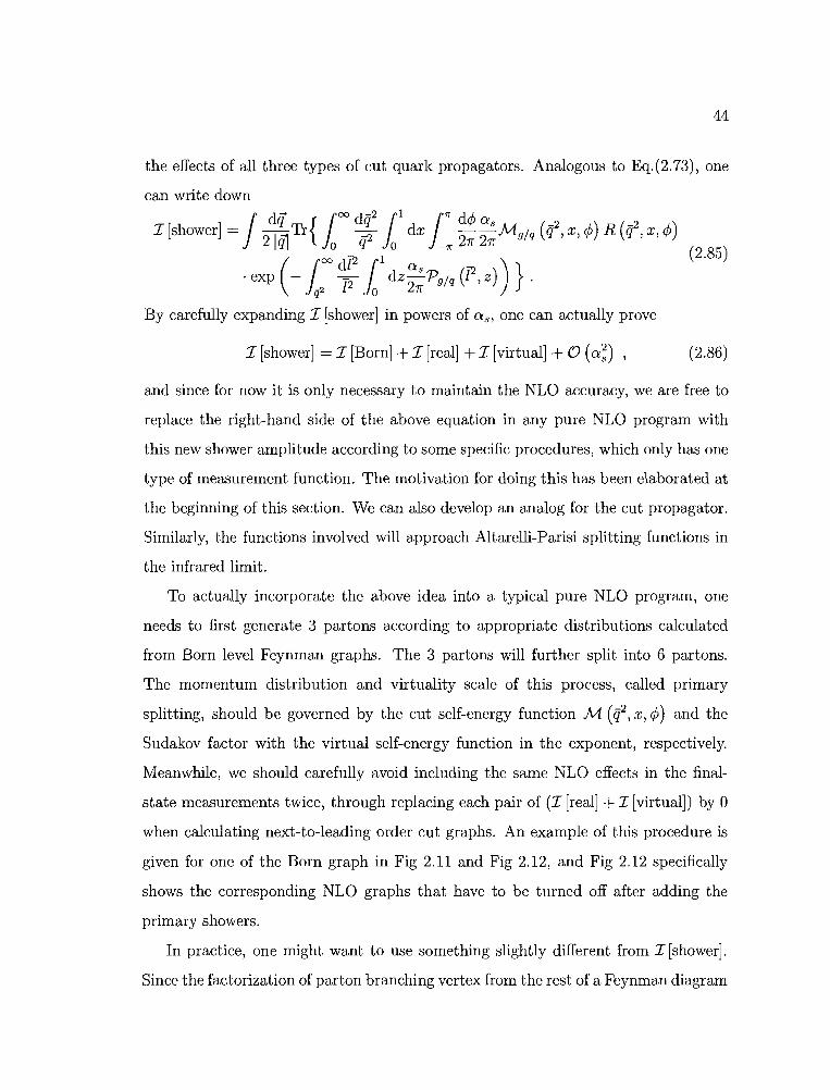
(2.85)
44
the effects of all three types of cut quark propagators. Analogous to Eq.(2.73), one
can write down
J dq roo dq2 t 111" d¢ aI[shower]= 21i]1Tr{io q2 io dx -11" 21f2;M g/ q (q2,X,¢)R(q2,X,¢)
(100 dP r1as 12)
. exp - iP [2 io dz 21f Pg/ q (l ,z) }.
By carefully expanding I [shower] in powers of as, one can actually prove
I [shower] = I [Born] + I [real] + I [virtual] + CJ (a;) , (2.86)
and since for now it is only necessary to maintain the NLO accuracy, we are free to
replace the right-hand side of the above equation in any pure NLO program with
this new shower amplitude according to some specific procedures, which only has one
type of measurement function. The motivation for doing this has been elaborated at
the beginning of this section. We can also develop an analog for the cut propagator.
Similarly, the functions involved will approach Altarelli-Parisi splitting functions in
the infrared limit.
To actually incorporate the above idea into a typical pure NLO program, one
needs to first generate 3 partons according to appropriate distributions calculated
from Born level Feynman graphs. The 3 partons will further split into 6 partons.
The momentum distribution and virtuality scale of this process, called primary
splitting, should be governed by the cut self-energy function M (q2, X, ¢) and the
Sudakov factor with the virtual self-energy function in the exponent, respectively.
Meanwhile, we should carefully avoid including the same NLO effects in the final
state measurements twice, through replacing each pair of (I [real] + I [virtual]) by 0
when calculating next-to-leading order cut graphs. An example of this procedure is
given for one of the Born graph in Fig 2.11 and Fig 2.12, and Fig 2.12 specifically
shows the corresponding NLO graphs that have to be turned off after adding the
primary showers.
In practice, one might want to use something slightly different from I [shower].
Since the factorization of parton branching vertex from the rest of a Feynman diagram
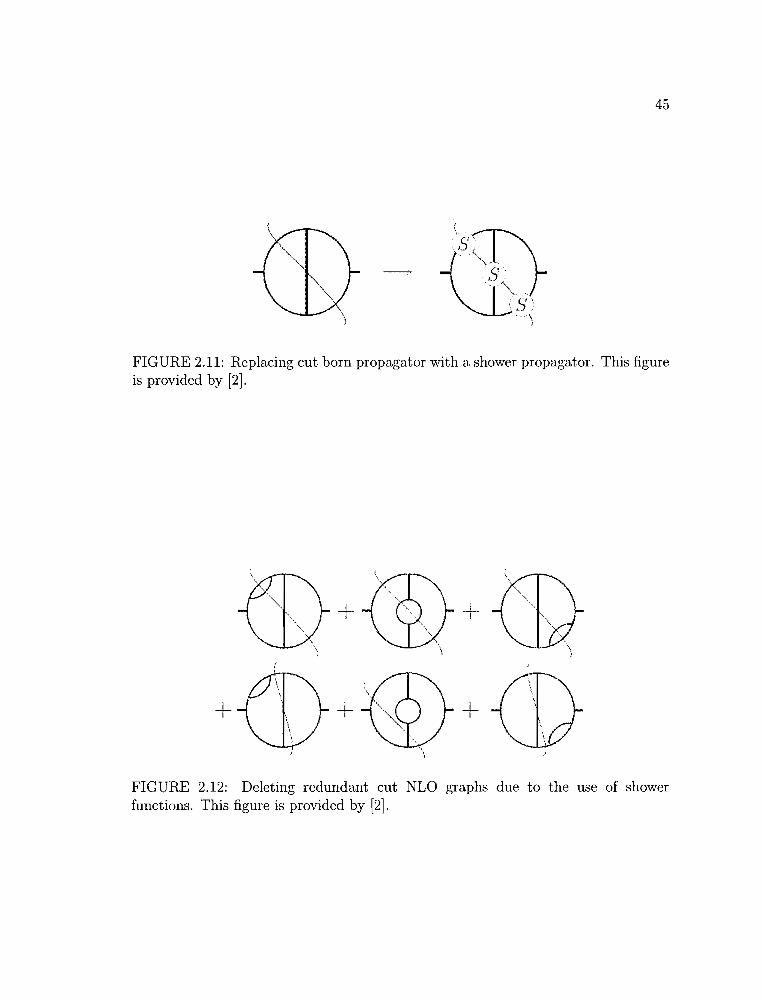
45
FIGURE 2.11: Replacing cut born propagator with a shower propagator. This figureis provided by [2].
+
+
+
+
+
FIGURE 2.12: Deleting redundant cut NLO graphs due to the use of showerfunctions. This figure is provided by [2].
46
is a good approximation only in the collinear region, it makes more sense if we cut
off parton splitting at a certain small scale so that the assumption of factorization
will not be violated when the program is processing primary showers, and put back
whatever pieces that have been missing from the modified shower algorithm, in the
form of ordinary cut lX; propagators. In detail, one can rewrite I [shower] as
J de] { lAver diP 1 1 171" d¢ lX s -2I[shower,.xv ]= 21",Tr ~ dx --Mg/q(q,x,¢)q I 0 q 0 -71" 27r 27r
( 100 df211 lX ).R(ii,x,¢)exp - 2"" dZ~Pg/q(p,z)},q;. l 0 27r
(2.87)
where .xvi! becomes the upper limit of the integration over the virtuality q2 of the
primary splitting instead of 00 in the original definition, and thus we would have a
corresponding leftover NLO piece to calculate, too:
J de] {lOO
dq211 171" d¢ lX s -2I [real, .xv] = 21'" Tr ~ dx --Mg/ q (q ,x, ¢)ql Avrr q 0 -71" 27r 27r
.R(q2,x,¢)} .
(2.88)
It can be easily proved the NLO accuracy will be intact if we include both
I [shower, .xv l and I [real, .xv l when modifying the primary shower algorithms.
2.5.2 Implementation
In original BEOWULF, a slightly different shower function is used to split Born
graph partons [2]. For example, a gluon is split into two other partons according to
(2.89)
where the trace is taken over Lorentz indices now, unlike the quark splitting case.
In order to preserve the NLO accuracy of the calculation, in addition to replacing
I [Born] with i [shower, .xv], one also has to replace I [real] and I [virtual] by
47
I [real, AvJ plus an infrared piece
(2.90)
(2.91)
M~V is the one-loop real gluon self-energy function calculated in Coulomb gauge,
and the loop could be either a gluon loop, or a quark loop running over all possible
flavors. In detail, it is a sum of four tensors [7J,
MJLV = as _1_ x {N D(Q -:1\JLV9 41f 1 + ~ TT , q)
+ N" [l~ -~D(Q,qr] + ~2NRRn"n"
N q . n (lJL v JLlV) }+ Et (1 +~) Q2 Tn + n T ,
where 1/ (1 +~) is a normalization factor (~== vII + rf/Q2 - 1), coefficients NTT ,
NUl NEE and NEt are functions of virtiality q2 and momentum fraction x, and
the tensor D (Q, iftV is the numerator of a bare on-shell gluon propagator with
momentum (Q, if), of which in the convention used here the only nonzero components
are D (Q, if)ij = !5ij with i,j E {1,2}. Among those coefficients, N u and NEt are of
less interest to us because they will vanish after integrating over angles; NEE will
not be written down here, either, since we are just interested in the q2 ----+ 0 limit, for
which the reason will given later. Now if we take this infrared limit, while ignoring
the coefficients mentioned above, we can obtain something similar to Eq. (2.79),
(2.92)
where Pg / g and Pq/ g are the one loop parton evolution kernals as defined in Sec. 2.4.2.
So the real gluon self-energy function we just gave does have the right behavior when
q2 ----+ O.
However, a different function M~v has been chosen to split the Born-level partons,
and one can obtain this function by replacing NTT with the simplified one-loop virtual
48
gluon self-energy function Pg (iP, x) (the exat form is given in [7]), and replacing NEE
with 0 in the real gluon self-energy function, as defined in Eq. (2.91). Based on the
explicit form of the virtual gluon self-energy function one can prove the following to
be true:
(2.93)
We will argue now the newly defined M~1I is indeed a good candidate as a gluon
splitting function. First of all, as implied by Eq. (2.90), which is a contribution
from the NLO leftover piece, the two subtracting terms are coupled with the
same measurement function. In pure NLO calculation, we also have a similar
NLO subtraction, but there different terms are associated with different final
states and thus when one needs to calculate differential cross sections, the infrared
cancellation will not be able to work properly in a single bin. This problem has
already been demonstrated in Fig 2.1. Secondly, by construction the remaining
NLO contribution after we split Born-level partons using M~1I is free of infrared
divergences. Furthermore, the new splitting function satisfies the probability
conservation. If one let the measurement function to be 1, then I [shower, AvJ of
Eq. (2.89) gives the total cross section. In this case RJ.L1I only depends on the virtuality
{p, and after integrating over the angle ¢ we could obtain the probability density of
gluon splitting to be
(2.94)
similar to Eq. (2.73).
Later we will see it is extremely difficult to generate splitting virtualities according
to the probability density given in last paragraph. In BEOWULF a standard Rejection
Sampling method is used, which is more sophisticated than the method discussed
earlier in this thesis. In Coulomb gauge, one can analytically calculate the virtual
49
gluon self-energy function. We use the following notations [2] for convenience:
where f.1 is the MS renormalization scale, and
2 _ . ( 2 1;;12)f.1mod = mm f.1 , qI
For gluon splitting to a quark and antiquark, one finds [2]
(2.95)
(2.96)
-2 1 1 iP { 16Pq/g(q ,x) =-{1-2x(1-x)}+-2-2- 2--x(1-x)2DJ1 2D1L f.1mod 3 (2.97)
+ log (f.12 / f.1~od) [1 - 2x (1 - x)] } .
For gluon splitting to two gluons, one finds
(-2 ) CA CA iP {Pg/g q,x =-{3x(1-x)-1}+-2-2- 7x(1-x)-2
DJ1 DJ1 f.1mod
+ log (f.12 / f.1~od) [3x (1 - x) - 1] }
12CA+ --x (1 - x){1 - 2x (1 - x)}D x
16CA { 2+ 152x (1 - x) 1 - 4x (1 - x) + 4 [x (1 - x)] }x
The virtual gluon self-energy function is
(2.98)
(2.99)
50
In Eq. (2.94), the integration of Pg over momentum fractions is straightforward to
calculate, and it will be called ~rue from now:
(2.100)
An auxiliary distribution is necessary to perform the Rejection Sampling algorithm,
and for this purpose BEOWULF makes up
'f -2 21 q < /-lmod
if q-2 > 1/2- rmod
(2.101)
where b is defined as
b == 1.1 X [6CA IcJ12
+ /-l~od (2NF _ 3CA) (8 + 3 log ( ~2 ))] ,5 18 /i'mod
and first sample points according to the probability density
(-2 ) _ as 1 (-2) (rOO d[2 as (1'2))Qapprox q ,00 = 21f if Papprox q exp - Jif [2 21f Papprox l ,
(2.102)
(2.103)
where the second argument of function Qapprox is the upper limit of the integral in
the exponent of the above equation. The algorithm used to get cP from Qtrue is to
use a series of probability densities which can be easily obtained by modifying only
the upper limit of the integration in the exponential of Eq. (2.103) to be a variable
ii. The procedure of sampling and rejecting is as follows:

(2)
51
FIGURE 2.13: The virtual gluon self-energy function is plotted as the black line,and the proposal function Papprox is plotted as the gray line.
(1) Sample a new random variable x from Qapprox (x, P) and u from a uniform
distribution in [0,1];
See if u < Ptrue (x) is true:Papprox (x)
(a) If true, then accept x as a sample point for ii;(b)
-2If false, then assign the value of x to k' , go back to step (1) and repeat
the algorithm, with the replacement of Qapprox (x, P) by Qapprox (x, k,2).
We initialize P to be 00 every time we begin sampling a new point for ii. The validity
of the above algorithm can be proved without much trouble. For simplicity, suppose
we only need to sample points in a finite region between 0 and q?nax, and divide this
region into N small pieces with the same size ~ == q?nax/N. The boundaries of those
small regions are denoted as q6, q~, ... ,qi, ... ,q'fv. Obviously, in the limit of N ---t 00,
the probability of getting an accepted point for q2 within [qi, qi+l] during the first
iteration is
Po
(2.104)

52
It is also not difficult to figure out the probability of getting an accepted point
within the same region [qf, qf+lJ during the second iteration is a sum of conditional
probabilities:
Q ( 2 2) ( Ptrue(ql+l)) Q (-2 -2 )approx qi+l' qmax . ~. 1 - P (-2)· approx qi' qi+l .~ .
approx qi+l~rue (qi)
Papprox (qi)
Q ( 2 2) ( P true (ql+2)) Q (-2 -2 )+ approx qi+2' qmax . ~. 1 - P (-2)· approx qi' qi+2 .~ .approx q,+2
~rue (qi)Papprox (qi)
+
+ Qapprox (q'tr, q~aJ . ~ . (1 - ;true (~~j)) .Qapprox (qf, q'tr) .~ .approx qN
(2.105)
If calculating probabilities like those given above for the rest iterations and summing
them up, one would obtain the Taylor expansion of
Qtrue (q;, q~aJ . ~ = q:? ;; P true (qi) exp (- l:~ax ~ ;;P true (P)), ~
. ~ , (2.106)
and therefore the validity of algorithm of sampling q2 according to Qtrue (ii, q~aJ is
proved.
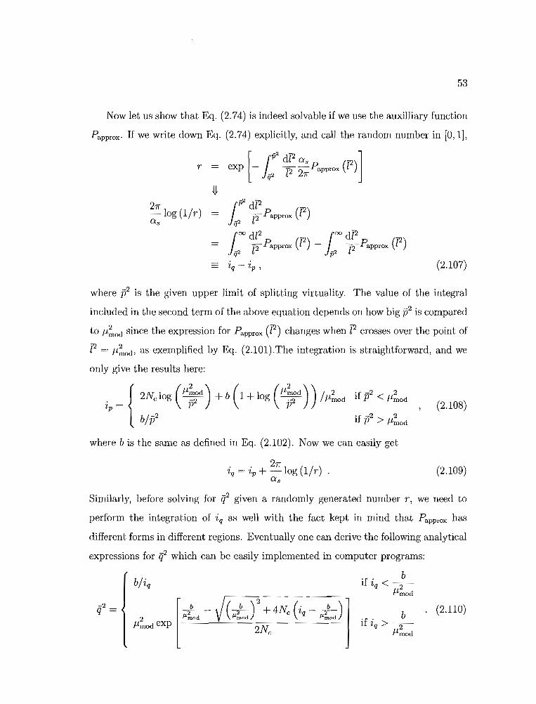
53
Now let us show that Eq. (2.74) is indeed solvable if we use the auxilliary function
Papprox' If we write down Eq. (2.74) explicitly, and call the random number in [0,1],
r
21f-log (l/r)as
[ l pz dr a ]exp - fP [2 2; Papprox ([2)
(2.107)
where ji is the given upper limit of splitting virtuality. The value of the integral
included in the second term of the above equation depends on how big tP is compared
to IL~od since the expression for Papprox (P) changes when P crosses over the point of
P = IL~od' as exemplified by Eq. (2.101).The integration is straightforward, and we
only give the results here:
ip
= { 2Nclog (IL;~d) + b (1 + log (IL;~d ) ) /IL~odbit}
if ji < IL~od
'f -2 21 P > ILmod
(2.108)
where b is the same as defined in Eq. (2.102). Now we can easily get
(2.109)
Similarly, before solving for {i given a randomly generated number r, we need to
perform the integration of i q as well with the fact kept in mind that Papprox has
different forms in different regions. Eventually one can derive the following analytical
expressions for {i which can be easily implemented in computer programs:
-2q =
r-Zb - (+)2 + 4Nc (i q - +-)]
2 Ilmod Ilmod IlmodILmod exp --..-----'----------
2Nc
'f . b1 ~q < -2-ILmod
bif i q > -2-
ILmod
. (2.110)
54
In addition to generating the splitting virtualities according to virtual self-energy
functions of partons in Coulomb gauge at one loop level with the help of auxilliary
functions, one also has to generate the right momentum distribution among the
splitting products. According to straightforward calculation of Feynman diagrams
under the assumption of collinear splitting as what we did earlier, the momentum
fraction of one of the two daughter partons, x, should obey some approximate
probability density distributions P(x). These functions are exactly the Alterelli
Parisi functions we have derived step by step. Thus naturally, we should be able to
generate the right momentum fractions using Eq. (2.75). However, because of the
complexities of some of the integrals of the virtual parton self-energy function over
the momentum fraction space, the above method is not well suited for numerical
calculations. To solve this problem, we will first introduce a very useful technique
called Importance Sampling.
Typically, importance sampling is frequently used to evaluate expectation values
at some distribution of interest that is not available or impractical for various
reasons. Importance sampling would generate random samples according to another
probability measure, but still manage to calculate the expectation values correctly.
Generally, suppose one wants to figure out the expectation of function J (x) given a
distribution p (x),
E[J(X) jp] == JJ(x)p(x)dx, (2.111)
what he can do is to generate random samples according to p, and take the following
to be an estimate of the real expectation after n iterations,
(2.112)
Sometimes the distribution of interest could be hard to generate numerically. Instead,
if one has another probability distribution q (x), namely the proposal distribution,
and still wants to calculate the same expectation, he could do use an another estimate
55
of the same integral by trivially rewriting Eq. (2.111) as below:
E[J(X)lp] = !!(X)P(x)dX
! ! (x) q(x) dxp(x)
E [! (X) I ]P (x) q ,
where
p(x) == q(x) /p (x) ,
(2.113)
(2.114)
and usually p-l is called the importance weight. So the estimate we are looking for
from samples produced according to the proposal distribution is
1 n
E[(J/p)lq] = - "L!(Xi)/p(X) .n
(2.115)
We can imagine by choosing proper importance weight one can optimize the numerical
integration, through avoiding enormous fluctuations of the integrand within the
region of integration.
In our case,BEOWULF uses a simple proposal distribution that is easy to calculate
the integral of, and thus samples can be generated straightforwardly by solving the
(2.75) repeatedly. In turn the integrand will have an extra factor of p- 1 that accounts
for the change in the distribution of random points. In more detail, the density of
sampling distribution is taken to be
() N(1 + fP/if)
q x '" c----:-'-----,-----'--.,---,---::-
2min (x, 1 - x) + if / if .(2.116)
up to a normalization factor. N c is the color factor of the splitting under investigation.
Obviously q(x) given above is invariant under the transformation x ---t 1 - x, and
it is because the distribution of two daughter partons in the momentum space is
symmetric. This sampling distribution does have a much simpler algebraic form and
thus Eq. (2.75) can be solved without too much programming efforts.
56
2.5.3 Numerical Tests
For practical reasons that have been stated many times earlier in this article,
we would like to develop even further showers from the partons after the primary
splittings, and finally generate hadrons instead of partons. It is the main motivation
for us to match the NLO matrix elements with parton showers and hadronizations. In
our case to do it properly, the shower history has to be recorded during the primary
splitting, because later the final state parton::> from the primary showering will become
the initial state of Pythia, a LO Monte Carlo program that generates parton showers
and hadronizations, and Pythia needs to know some necessary information [9] to
kick off further evolutions of the hard~st partons, such as parton flavors, color
configuration, hardness scale of the last splitting, etc. Eventually events with physical
particles can be generated by Pythia, but this time calculations done based on those
events will be accurate to the next-to-Ieading order as we will confirm below, and
thus we say this type of calculation is carried out in the mode of NLO + PS + Had.
Similarly, if we only use Born graphs with showers and hadronization, we shall refer
to this mode as LO + PS + Had. We also perform calculations from a pure lowest
order perturbative calculation, LO, from a pure next-to-Ieading order perturbative
calculation, NLO, and from the program Pythia itself.
There are several things to be examined before one can confirm this program's
validity. First of all, we need to make sure the calculation in the mode of NLO + PS
is indeed accurate to the order of a;. Let us make use of the results of 3-jet fraction
in different modes, and construct the following ratio [9],
R[NLO PS] = is [NLO + PS] - is [NLO]+ is [NLO]
(2.117)
This ratio should have a perturbative expansion starting at order a;. The rationale
is that the difference of is [NLO + PS] and is [NLO] should start at order a; if
the matching of parton showers to the matrix elements is done correctly. The
denominator, the 3-jet fraction of NLO alone, apparently begins at order as, since
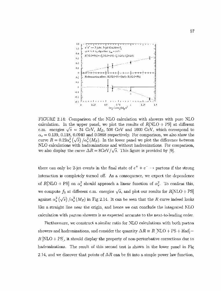
57
-
0.6c-r-T"""T"TT"....-r--.-r-,--,--.--r-r-r-r........-r....-r---.--r--,--,---,--..--:J
('.~ f- e~e- - .3 jets: 3-jet fractiol~ (,0.4 i~t = ..;-., 6. kr algorithm. Y,tm = (t.05!
W"LO+PSj =d,l~lo-PSI·f;I~LOI) i;[~lOi
-.. j"
..•... 1···· .. ·1-!-·1-··1
1 1
(> H'-'+-+-++I+-t-H-fI-H-I-1-H-1 +-+-++1+-t-t-t-fI-+-I-I-HHadronlz;"lti~.u~f!~t't~. RfXLO-PS-Hadj . Rt'xLO":'PSl0,;
0,1
Q.]
T
'0.~i E-F'-~-----~'-of. ."".oir· ::-.--'-"'-"-.-l"T..-...-.-...-...----:J-'
·0; b "1' --0.2: c..L.L-.L.L..L--L.L.l.l.--.L-1--"...JIL,IL.L-1.1...11-'1-1-LI.-'-1.-'-,..1-1~'-'-'...lI...LI...JILL.L:J
(0 o.;~ 05 (I-.t:;
((i!>i \-) -;;-(I.~( ~dz»),~1.25
FIGURE 2.14: Comparison of the NLO calculation with showers with pure NLOcalculation. In the upper panel, we plot the results of R[NLO + PS] at differentc.m. energies VS = 34 GeV, Mz , 500 GeV and 1000 GeV, which correspond toas = 0.139, 0.118, 0.0940 and 0.0868 respectively. For comparison, we also show thecurve R = 0.22a; (VS) la; (Mz). In the lower panel we plot the difference betweenNLO calculations with hadronizations and without hadronizations. For comparison,we also display the curve t1R = 8GeVIvs. This figure is provided by [9].
there can only be 2-jet events in the final state of e+ + e- ---t partons if the strong
interaction is completely turned off. As a consequence, we expect the dependence
of R[NLO + PS] on a; should approach a linear function of a;. To confirm this,
we compute 13 at different c.m. energies VS, and plot our results for R[NLO + PS]
against a; (VS) la; (Mz) in Fig 2.14. It can be seen that the R curve indeed looks
like a straight line near the origin, and hence we can conclude the integrated NLO
calculation with parton showers is as expected accurate to the next-to-Ieading order.
FUrthermore, we construct a similar ratio for NLO calculations with both parton
showers and hadronizations, and consider the quantity t1R = R [NLO + PS + Had]
R [NLO + PS], it should display the property of non-perturbative corrections due to
hadronizations. The result of this second test is shown in the lower panel in Fig
2.14, and we discover that points of t1R can be fit into a simple power law function,
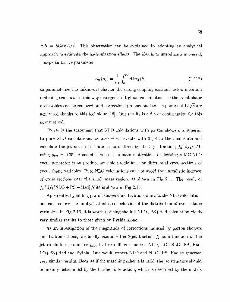
(2.118)
58
b.R = 8GeVI /S. This observation can be explained by adopting an analytical
approach to estimate the hadronization effects. The idea is to introduce a universal,
non-perturbative parameter
1 11L1
Qo (I1I) = - dkQ s (k)/1'I 0
to parameterize the unknown behavior the strong coupling constant below a certain
matching scale I1I' In this way divergent soft gluon contributions to the event shape
observables can be removed, and corrections proportional to the powers of 1//S are
generated thanks to this technique [16]. Our results is a direct confirmation for this
new method.
To verify the statement that NLO calculations with parton showers is superior
to pure NLO calculations, we also select events with 3 jet in the final state and
calculate the jet mass distributions normalized by the 3-jet fraction, f3-1dh/dM,
using Ycut = 0.05. Remember one of the main motivations of devising a MC-NLO
event generator is to produce sensible predictions for differential cross sections of
event shape variables. Pure NLO calculations can not avoid the unrealistic increase
of cross sections near the small mass region, as shown in Fig 2.1. The result of
f:;ldh [NLO + PS + Had] IdM is shown in Fig 2.15.
Apparently, by adding parton showers and hadronizations to the NLO calculation,
one can remove the unphysical infrared behavior of the distribution of event shape
variables. In Fig 2.16, it is worth noticing the full NLO+PS+Had calculation yields
very similar results to those given by Pythia alone.
As an investigation of the magnitude of corrections induced by parton showers
and hadronizations, we finally examine the 3-jet fraction h as a function of the
jet resolution parameter Ycut in five different modes, NLO, LO, NLO+PS+Had,
LO+PS+Had and Pythia. One would expect NLO and NLO+PS+Had to generate
very similar results. Because if the matching scheme is valid, the jet structure should
be mainly determined by the hardest interaction, which is described by the matrix
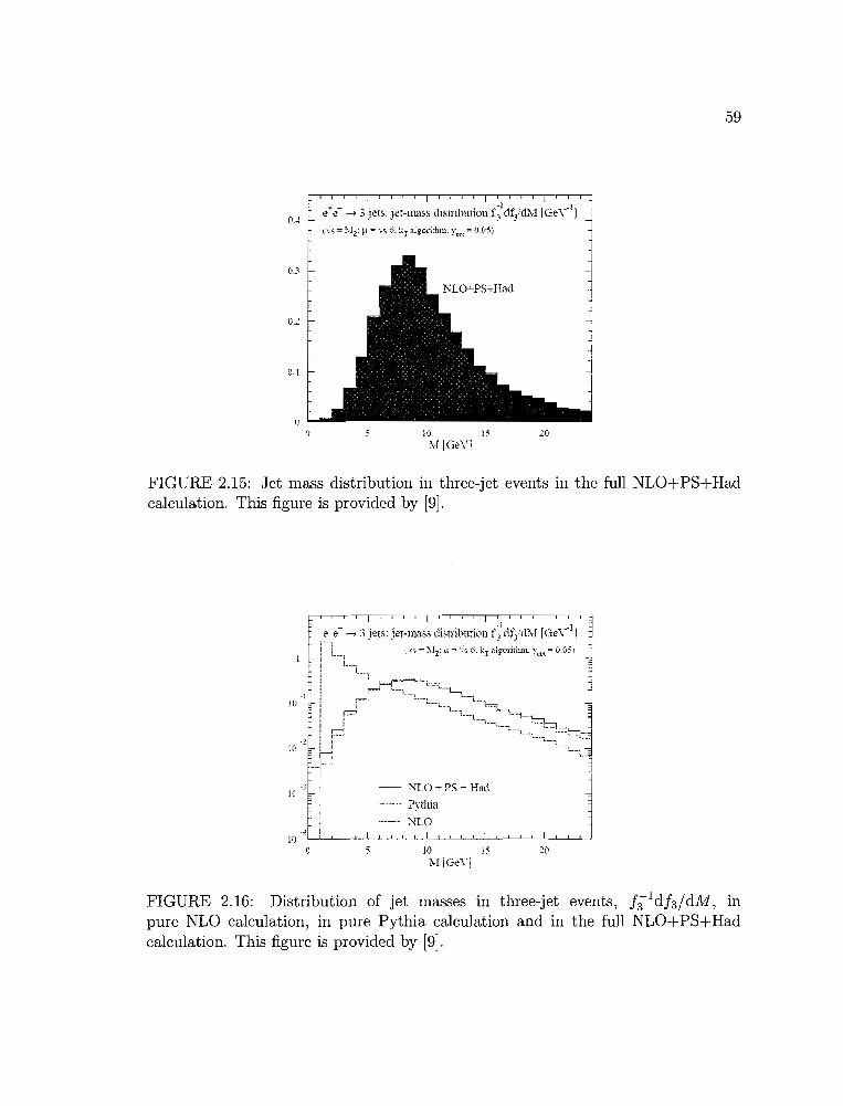
0.-4e~e- ~ 3 jets: jet-Illa" di>rribmion f~J dl~d\f IGe\-·llI ".;.~ = ~'lz: p = 'i'~ '0. k1 alg-ofltlull, Yet" ={i.0:')
59
<) 10 1~
AIIGeV]20
FIGURE 2.15: Jet mass distribution in three-jet events in the full NLO+PS+Hadcalculation_ This figure is provided by [9].
-- NLO';'PS~Hacl
PythiaNLO
10 15 .20MiGe\-1
FIGURE 2.16: Distribution of jet masses in three-jet events, f3-1dh/dM, inpure NLO calculation, in pure Pythia calculation and in the full NLO+PS+Hadcalculation. This figure is provided by [9].
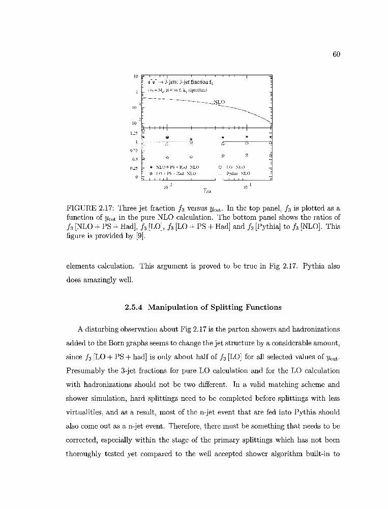
10 ~ I~. ~- --> 3 j~ts: 3-j~t ii-action f;
1 ~ (\:'s = ~lz' J-l = >~~ 6. kr r;lgorirhm i
() LO. "LO
PythKl NLO
-I](J ...
ll'
1.2< :0'
l*c..
I}:.:o- t-
O.:' ~
0.2<
I
'" i!..
L .'J C
f~ it 'fJ
.. "L() • PS - Kld "LO
1< LO" PS - Had "LO
-2j(,
60
I -';
..,
-,-" ....---
......, ........
I'-~
* ~
--::
-·1
10
FIGURE 2.17: Three jet fraction h versus Ycut. In the top panel, h is plotted as afunction of Ycut in the pure NLO calculation. The bottom panel shows the ratios ofh [NLO + PS + Had], h [La], h [La + PS + Had] and h [Pythia] to h [NLO]. Thisfigure is provided by [9].
elements calculation. This argument is proved to be true in Fig 2.17. Pythia also
does amazingly well.
2.5.4 Manipulation of Splitting Functions
A disturbing observation about Fig 2.17 is the parton showers and hadronizations
added to the Born graphs seems to change the jet structure by a considerable amount,
since h [La + PS + had] is only about half of h [La] for all selected values of Ycut.
Presumably the 3-jet fractions for pure La calculation and for the La calculation
with hadronizations should not be two different. In a valid matching scheme and
shower simulation, hard splittings need to be completed before splittings with less
virtualities, and as a result, most of the n-jet event that are fed into Pythia should
also come out as a n-jet event. Therefore, there must be something that needs to be
corrected, especially within the stage of the primary splittings which has not been
thoroughly tested yet compared to the well accepted shower algorithm built-in to
61
Pythia. The magnitude of the deviation of h [LO + PS + had] from h [LO] can be
estimated by considering a factor of [1 - X as (VS/6) ], which is brought up every
time a primary splitting is added to a cut parton propagator in the LO Feynman
diagrams and change the normalization by an amount proportional to as (VS/6).
Qualitively, since there are three cut propagators in such graphs, one can therefore
approximately predict that
h [LOf:[~~t had] ~ [1 - Xa s (VS/6)]3 , (2.119)
where the coefficient X is determined by the splitting functions that we use in the
matching algorithm. With the c.m. energy chosen to be 91GeV and thus as (VS/6) ~
0.16, we conclude this branching coefficient X must be rv 1.5 in order to produce
what we see in Fig 2.17. Obviously one could make X much closer to zero in order to
resolve this problem, and our remedy is of course to adopt different splitting functions
for the primary splittings. Following the same logic behind Eq. (2.87) and Eq. (2.88),
in the calculation of shower amplitude I [shower, Av] we choose to replace the one
loop self-energy function M with a new function, whose form will be restricted later,
and to leave the Sudakov exponential untouched. Through some treatment on the
propagators of corresponding NLO graphs, the NLO calculations with parton showers
will remain equivalent to the pure NLO calculations, up to a slightly different NNLO
(Next-to-Next-Leading Order) correction. However, the LO calculations with parton
showers can vary a lot as we split the hard partons according to different functions.
We can hence make use of the sensitivity of I [shower, Av] to the choice of splitting
functions, and justfy the reliability of the resulting primary splitting. If one can bring
h [LO + PS + had] and h [LO] closer to each other, we would be able to preserve
the virtuality hierarchy inherent with the parton shower algorithm, and keep the
approximations made in such an algorithm relevant.
In order to put constraints on a valid splitting function that substitutes M, we
need to remind ourselves about how to keep NLO calculations with showers accurate
(2.120)
62
to the next-to-leading order. Suppose we replace function M and P in the shower
amplitude I [shower] with different functions M ' and p'. The cut on shower scales
has been omitted here from the amplitude deliberately for simplification. In the
calculation of NLO matrix elements, we need to use M - M ' instead of M alone to
represent the cut one-loop self-energy function, and use P - p' instead of P alone to
represent the virtual one-loop function, so that partons can develop primary showers
without undermining the program's NLO accuracy. One special example is when
M ' = M and p' = P, NLO graphs that contain such cut propagators are simply
removed calculation. According to this argument, even if the two sets of splitting
functions are different, the function with its pairing substitute still has to have the
same IR limit. This is because both P and Pare IR divergent. Also M - M ' and
P - p' shall be integrated to zero virtuality, and both subtractions have to be free of
infrared divergences in order for the numerical integration to converge fast enough.
The last paragraph is basically a recapitulation of the Sec. 2.5.2. In that section,
the virtual parton self-energy function P is used to replace the coefficient of the non
vanishing transverse component of the cut parton self-energy function, and as a result,
cancellations of some of the IR divergences in NLO graphs are achieved, because
the constraint on new splitting functions explained in last paragraph is satisfied.
However, this specific implementation of shower scheme could only give us results
displayed in Fig. 2.17. Through further investigation and repetitive trials, we find
that by putting a factor
(-2 ~) Aq2
C q ,q = 1 + Br;2 ;;2q +q
in front of the term including P in the definition of cut parton self-energy function,
and by using this modified function to split Born-level partons, one can effectively
enhance parton branching and convert more 2-jet events to 3-jet events because the
additional factor is always greater than 1. Meanwhile, one can also retain the same

63
0
1.2
1.0 *[, "!!. :,
0 0.8-'Z:;:, ..Q) 0.6 "Cla::;;;:'-, 0.4
0.2
0.00.01
."
* NLO+PS+HadiNLO" LO+PS+Had i NLOo LO!NLO{', Pythia! NLO
0.1
FIGURE 2.18: Three jet fraction h versus Ycut. The plot shows the ratios ofh [NLO + PS + Had]' h [LO], h [LO + PS + Had] and h [Pythia] to h [NLO], witha modified splitting function.
IR limit of the splitting function if the virtuality goes to zero for fixed rf. In the
latest version of program BEOWULF, we set
{A = 2.0 ,
B =4.0(2.121)
and test our choice of parameters by once again plotting the ratios of 3-jet fractions
in different modes to the same observable calculated by pure NLO calculations. The
results are shown in Fig. 2.18.
In Fig. 2.18, there are several things that are different from the old graph in
Fig. 2.17. First of all, compared to the results generated by using old splitting
functions, the values of h [LO + PS + Had] are now brought much closer to the
pure LO values by switching to the modified splitting functions. The ratio of
h [LO + PS + Had] to h [NLO] has become 60% rv 80% as the chosen jet resolution
parameter Ycut varies from 0.002 to 0.2. As the smaller Ycut one uses, the better
resolution one would have over jet finding. Therefore, if there are a lot of 3-jet

64
events that contain a jet which could be identified as two seperate jets, the trend
of fa [LO + PS + Had] growing as Ycut increases would be able to well explained.
However, we still can not understand why LO calculation with hadronization would
develop more events of this type than the rest of the modes. Another improvement
displayed by Fig. 2.18 over the old graph is that NLO calculation with hadronizations
are now yielding fa more consistently with the pure NLO calculation. The average
difference between fa [NLO + PS + Had] and fa [NLO] was around 10%, and a
systematic deviation was implied since fa [NLO + PS + Had] was universally greater
than fa [NLO] for different jet resolution parameters. After the splitting functions
are modified, the average difference between those two quantities has been reduced
to less than 5%, and the unpleasant systematic deviation seems to vanish. This
observation also justifies the change made to the primary splitting in BEOWULF.
A variety of tests, such as those that have been done on the old program, can also
be performed on the modified program in order to examine its NLO accuracy, ability
to deal with differential cross sections, etc., but those tests shall be removed from
further discussion here because of the similarity displayed in the results. Instead, we
study the program's dependence on the choice of splitting functions. A number of
different 3-jet infrared-safe observables are picked for this purpose. We will show the
program with modified splitting functions is superior. Before that, we first need to
introduce some fundamentals of useful event-shape variables.
2.6 Event Shape Variables
This brief introduction is about how to calculate different eventshape variables
of hadronic final states of electron-positron annihilations, including jet production
rates, Thrust, Thrust Minor and Major, Oblateness, C-Parameter, Spherocity, jet
masses, the jet broadening measures, energy correlations. Earlier, we have already
frequently used the concept "3-jet fraction" many times, without seriously defining
65
what exactly a "3-jet event" refers to. So we will start with defining such an event,
and also discuss several different ways to constrain the jet resolution.
2.6.1 Jet Algorithms
Let us take the "minimum invariant mass" or JADE algorithm as an example.
Consider qqg production at O(Qs), e.g., with three partons in the final state. In
this specific algorithm, a three-jet event is defined as one in which the minimum
invariant mass of the parton pairs is larger than some fixed resolution constant
Y (sometimes called Ycut) of the overall center-of-mass energy:
(2.122)
More jet-finding algorithms and definitions of their corresponding resolution
parameters are listed in Table 2.4. Generally speaking, such algorithms always begin
with calculating the resolution values for every possible pair of final-state particles.
The next step is to compare the minimum resolution values with the fixed resolution
parameter Ycut. If Ycut is greater than this minimum value, one should first proceed
to combine the two particles that correspond to the minimum value according to
rule of combining displayed in Table 2.4, and then treat the combined particles as
a single new particle when finding the new minimum resolution value during the
next cycle. If Ycut is smaller, however, one should instead terminate the current
jet-finding algorithm, and the jet structure of the current cycle will be used as the
finalized jet structure.
2.6.2 Thrust-Related Variables
The following variables are either the variable of Thrust itself, or variable which
must be defined with the help of thrust-axis. We will start with defining the variable
Thrust.
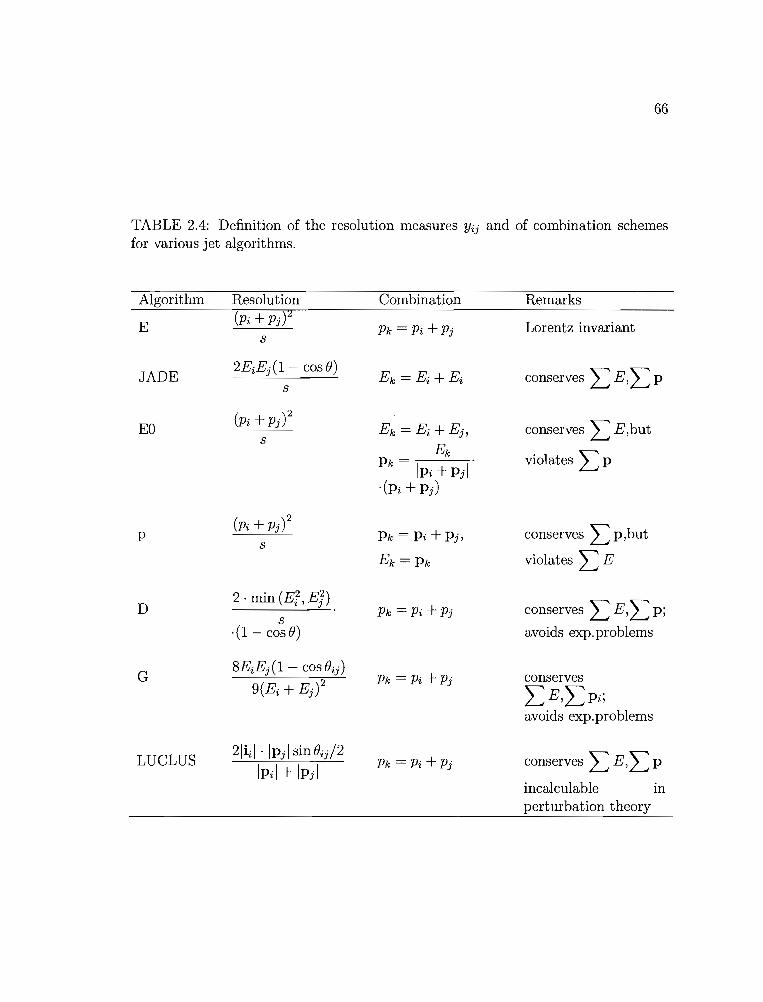
66
TABLE 2.4: Definition of the resolution measures Yij and of combination schemesfor various jet algorithms.
Algorithm Resolution Combination Remarks
E(Pi + pj)2
Pk = Pi +Pj Lorentz invariants
JADE2EiEj (1 - cos e)
E k = Ei + Ei conserves L E, L Ps
EO(Pi+Pj)2
E k = Ei +Ej , conserves L E,buts
Ekviolates LPPk = .
IPi + pjl.(Pi + Pj)
P(Pi+Pj)2
Pk = Pi + Pj, conserves L p,buts
E k =Pk violates LE
2· min (E2 E~)conserves L E'L P;D " J Pk = Pi +Pjs
·(1 - cos e) avoids expo problems
G8EiE}(1 - cos (}ij)
Pk = Pi +Pj conserves9(Ei + Ej )2
LE'LPi;avoids exp.problems
LUCLUS2liil· !pjl sin (}ij/2
Pk = Pi +Pj conserves L E,L PIPil + Ipjl
incalculable mperturbation theory

(2.123)
67
2.6.2.1 Thrust T
The thrust value of a hadronic event is defined by the expression
(L::i Ipi .nl)
T = m:x L::i Ipil .The vector nwhich maximizes the expression in parenthesis is the thrust axis nT. It
is used to divide an event into two hemispheres HI and Hz by a plane through the
origin and perpendicular to the thrust axis.
2.6.2.2 Thrust-Major
Given the thrust axis nT which maximizes the sum in equation (2.123), the thrust
major is defined as
(2.124)
where the vector n, the thrust major axis, obviously lies in the plane perpendicular
to the thrust axis.
2.6.2.3 Thrust-Minor
At this point, we define the event plane to be the plane spanned by the thrust
axis and the thrust major axis as the yz-plane, and a unit vector along the x-axis
would be nmin = nT x n. And the thrust minor, which measures the radiation out of
the event plane, can be defined as
(2.125)
2.6.2.4 Oblateness
Given the thrust major and thrust minor defined above, the oblateness is given
by
68
(2.126)
2.6.2.5 Heavy Jet Mass M H
From the particles in each of the two hemispheres defined by the thrust axis an
invariant mass is calculated. The heavy jet mass MH is defined to be the larger of the
two jet masses. The original analysis by S.Bethke used the measured heavy jet mass
scaled by the visible energy Evis which is, after correction for detector resolution,
acceptance, and for initial state radiation, equal to MH/v's. More specifically, in
any event, as for the two hemispheres of particles divided by the thrust axis nT, we
call the right one R, and the left one L. The squared heavy jet mass is defined as
(2.127)
where M~,M'i are the single hemisphere sqared masses normalized to be
dimensionless
( )
2
M 2 = L PiL - iEL 2:j lfijl
(2.128)
2.6.2.6 Jet Broadening B
The jet broadening measures are calculated by the expression:
(2.129)
for each of the two hemispheres, H k , defined above. The total jet broadening is given
by BT = B 1 + B2 . The wide jet broadening is defined by Bw = max(B1 , B 2 ).
69
2.6.3 C-Parameter
The C-Parameter is defined as
(2.130)
where AI" 'Y = 1,2,3, are the eigenvalues of the momentum tensor
(2.131)
The book
enfj = I:i pypfj IPi I.I:j Ipj/
QCD and Collider Physics [10] gives an algebric expression of the C-
Parameter, which is equation (3.41):
c = ~I:i,j [IPillpjl- (Pi· pj)2/IPillpjl]2 (I:i IPi 1)2
(2.132)
The two above definitions of C-Parameter are equivalent to each other. The proof is
given below.
First, take the trace of the momentum tensor (2.131), we could find the following:
(2.133)
which leads to
Therefore, the C-Parameter can also be expressed as
c = ~ [1 - (Ai + A~ + AD]
(2.134)
(2.135)
Because e is real and symmetric, it can be diagonalized through orthogonal
transformation, u-1eu = D. D is the resulting diagonal matrix, and its diagonal
elements are the common eigenvalues of both matrices. The quantity Ai + A~ + A~

70
can be seen as the trace of the square of matrix D 2 . Since D 2 = U- 18U . U- 18U =
U- 18 2 U, we could say
(2.136)
Now, let us write down Tr8 2 explicitly in terms of the final state momentum:
Tr8 2 = L 8 a,B8,Baa,,B
= L Ei~pf!IPiI .E j t!jfJjjlPi Ia,,B Ej Ipl I E j Ipl I
Eij [(Pi' Pi)2/IPiIIPiI]
(Ej IPilr
From here, we can derive
(2.137)
(2.138)
So we have proved the above two definitions of C-Parameter are indeed equivalent.
2.6.4 Spherocity
The spherocity of a certain event is defined as
S = (i)2 . (Ei IPi x itl)2mln '" I_I .
1r n Di Pi(2.139)
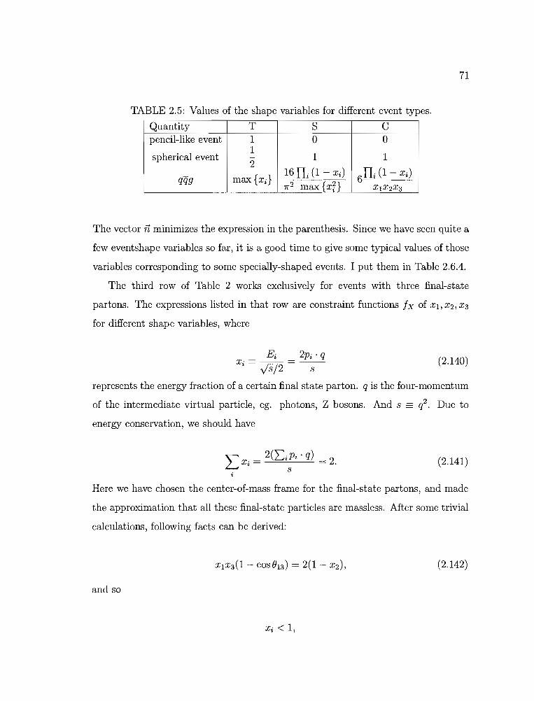
(2.140)
71
TABLE 2.5: Values of the shape variables for different event types.
Quantity T S Cpencil-like event 1 0 0
spherical event1
1 1-
2
qqg max {Xi}16 rt (1- Xi) 6ft (1 - Xi)
7[2 max {x~} XIX2 X 3
The vector nminimizes the expression in the parenthesis. Since we have seen quite a
few eventshape variables so far, it is a good time to give some typical values of those
variables corresponding to some specially-shaped events. I put them in Table 2.6.4.
The third row of Table 2 works exclusively for events with three final-state
partons. The expressions listed in that row are constraint functions Ix of XI, X2, X3
for different shape variables, where
Ei 2pi·qx·=-----• - y's/2 - s
represents the energy fraction of a certain final state parton. q is the four-momentum
of the intermediate virtual particle, ego photons, Z bosons. And s == q2. Due to
energy conservation, we should have
(2.141)
Here we have chosen the center-of-mass frame for the final-state partons, and made
the approximation that all these final-state particles are massless. After some trivial
calculations, following facts can be derived:
(2.142)
and so
Xi < 1,
72
At O(as), the distribution of total cross-section in the shape variable do)dX
(X=T,S,... ) is obtained by integrating the right-hand side of
(2.143)
(2.144)
z.e. along a contour in the (Xl, X2) plane. Other than that, there is something else
that needs to be noticed here. As long as the variables are not equal to their pencil
like limits, e.g., T < 1, then those distributions are finite, since the soft and collinear
configurations are excluded from the integration range [10]. I mentioned the above
point because there are some shape variables whose calculations could involve soft
and collinear singularities, like the energy-energy correlation junction (EEG), which
I will talk about next.
2.6.5 Energy-Energy Correlation Function
EEC is a dimensionless angular distribution defined by
1 dE
o dcos X
(2.145)
where E I E2rJ!5(j / d3pI d3
p2 is the two-hadron inclusive cross section. The first sum on
the right-hand side is over all distinct pairs of hadrons-n(n - 1)/2 terms for an
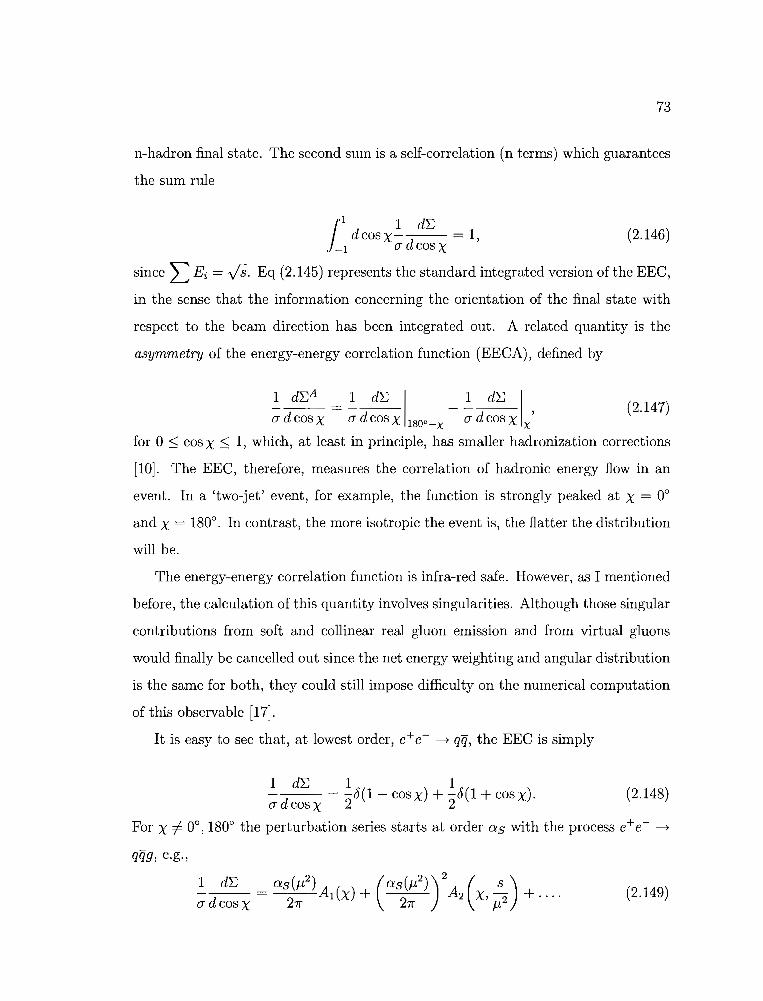
(2.146)
73
n-hadron final state. The second sum is a self-correlation (n terms) which guarantees
the sum rule
11 1 d'BdcosX- d = 1,
-1 (J cos X
since LEi = .;s. Eq (2.145) represents the standard integrated version of the EEC,
in the sense that the information concerning the orientation of the final state with
respect to the beam direction has been integrated out. A related quantity is the
asymmetry of the energy-energy correlation function (EECA), defined by
1 d'BA
1 d'B I 1 d'B I- - - - - (2.147)(JdcosX - (JdcosX 1800-x (JdcosX x'
for 0 ::; cos X ::; 1, which, at least in principle, has smaller hadronization corrections
[10]. The EEC, therefore, measures the correlation of hadronic energy flow in an
event. In a 'two-jet' event, for example, the function is strongly peaked at X = 00
and X = 1800• In contrast, the more isotropic the event is, the flatter the distribution
will be.
The energy-energy correlation function is infra-red safe. However, as I mentioned
before, the calculation of this quantity involves singularities. Although those singular
contributions from soft and collinear real gluon emission and from virtual gluons
would finally be cancelled out since the net energy weighting and angular distribution
is the same for both, they could still impose difficulty on the numerical computation
of this observable [17].
It is easy to see that, at lowest order, e+e- ~ q7j, the EEC is simply
1 d'B 1 1- d = -20(1 - cos X) + -0(1 + cos X)· (2.148)(J cos X 2
For X =I- 00, 1800 the perturbation series starts at order as with the process e+e- ~
q7jg, e.g.,
(2.149)
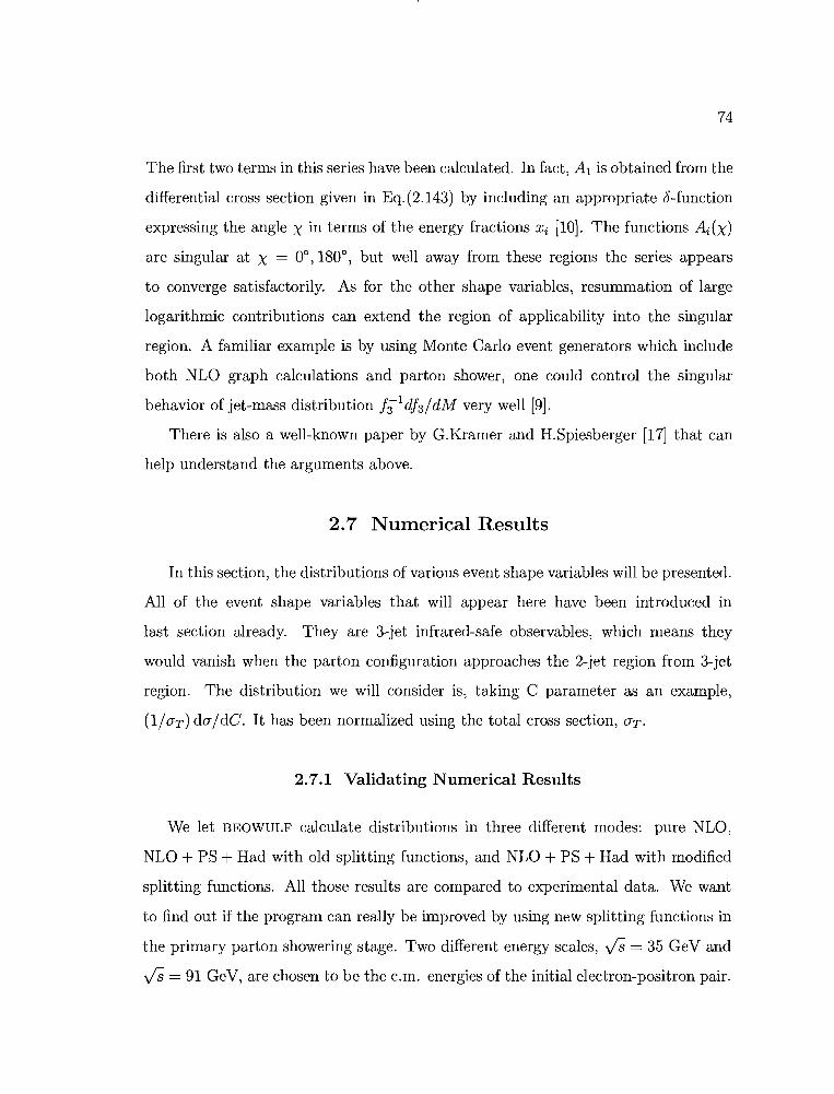
74
The first two terms in this series have been calculated. In fact, Al is obtained from the
differential cross section given in Eq. (2.143) by including an appropriate 6-function
expressing the angle X in terms of the energy fractions Xi [10]. The functions Ai(X)
are singular at X = 00, 1800
, but well away from these regions the series appears
to converge satisfactorily. As for the other shape variables, resummation of large
logarithmic contributions can extend the region of applicability into the singular
region. A familiar example is by using Monte Carlo event generators which include
both NLO graph calculations and parton shower, one could control the singular
behavior of jet-mass distribution f:;ldh/dM very wen [9].
There is also a well-known paper by G.Kramer and H.Spiesberger [17] that can
help understand the arguments above.
2.7 Numerical Results
In this section, the distributions of various event shape variables will be presented.
All of the event shape variables that will appear here have been introduced in
last section already. They are 3-jet infrared-safe observables, which means they
would vanish when the parton configuration approaches the 2-jet region from 3-jet
region. The distribution we will consider is, taking C parameter as an example,
(l/iTT) diT/dC. It has been normalized using the total cross section, iTT.
2.7.1 Validating Numerical Results
We let BEOWULF calculate distributions in three different modes: pure NLO,
NLO + PS + Had with old splitting functions, and NLO + PS + Had with modified
splitting functions. All those results are compared to experimental data. We want
to find out if the program can really be improved by using new splitting functions in
the primary parton showering stage. Two different energy scales, VB = 35 GeV and
VB = 91 GeV, are chosen to be the c.m. energies of the initial electron-positron pair.

75
30
-25
~..... 20.g-15
~..... 10r-l
5
•
•
",
••
•"
pure NLO calculation
~ = Mz , J.l = ~/6
o 0.05 0.1 0.15l-T
0.2 0.25
FIGURE 2.19: Thrust distribution. Experimental data is compared with thenumerical results for Pure NLO (91 GeV).
In principle, more serious long distance effects should be present at the lower energy,
which would obviously compromise the ability of pure NLO calculation to describe
the shape of final states. However, non-perturbative effects can be accounted for by
developing parton showers and hadronizations. We want to find out if parton showers
and hadronizations can indeed be more helpful at the lower energy of the two. In this
project, we use the experimental data presented in [18][19:1[20]. We choose to study
the distributions of Thrust, Total Jet Broadening measure, Wide Jet Broadening
measure, Heavy Jet Mass and C Parameter due to the availability of experimental
data at 35 GeV.

76
••
!.••
0.40.3
e+e- ~ 3 jets, Thrust
pure NLO ca1cu~ation
~ = 35 GeV, ~ = ~/6
"0.2
l-T0.1
17.5
15......E-l"0 12.5
" •tl 10"0 •6' -7.5
" •r-I 5
2.5
•0
FIGURE 2.20: Thrust distribution. Experimental data is compared with thenumerical results for Pure NLO (35 GeV) .
•
•
•
•0.250.2
•
NLO+PS+Had, old
e+e- ~ 3 jets, Thrust
•
0.1 0.15l-T
•
0.05
• I• I
17.5
15......E-l"0 12.5
"b 10"0
Eo< 7.5b
"r-I 5
2.5•
0
FIGURE 2.21: Thrust distribution. Experimental data is compared with thenumerical results for NLO + PS + Had with old splitting functions (91 GeV).
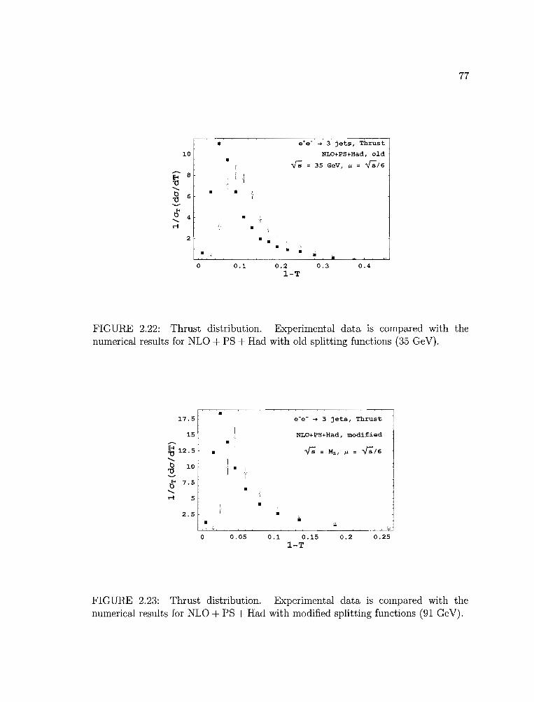
77
•
••
e+e- ~ 3 jets, Thrust
NLO+PS+Had, old
,(; = 35 GeV, ~ = ,(;/6
0.4•
0.3
•• ••
0.2l-T
•
0.1
•10
•--- 8E-l'0....... •tl'0 6
t5' 4.............
2
.,0
FIGURE 2.22: Thrust distribution. Experimental data is compared with thenumerical results for NLO + PS + Had with old splitting functions (35 GeV).
••
• I
I
!• I
•
,.--~-.~~~~~---~--~--~
e+e- ~ 3 jets, Thrust j
NLO+PS+Had, modified 1
J,I'Y;=Mz,~=Y;/6 1
11
15
17.5
E-l'0 12.5........g 10
t5' 7.5............. 5
2.5
•• •
o 0.05 0.1 0.15l-T
0.2 0.25
FIGURE 2.23: Thrust distribution. Experimental data is compared with thenumerical results for NLO + PS + Had with modified splitting functions (91 GeV).
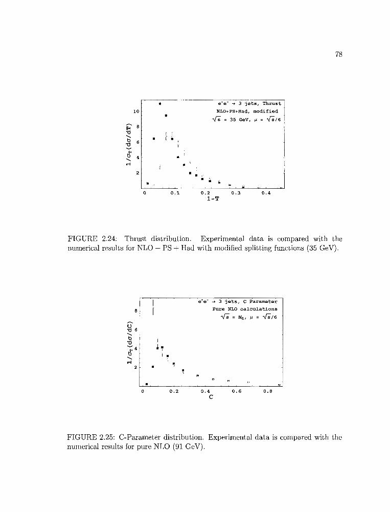
10
2
•
,•
I r
• I •
••
• •
e+e- ~ 3 jets, Thrust
NLO+PS+Had, modified
~ = 35 GeV, ~ = ~/6
•• IIIi
78
o 0.1 0.2I-T
0.3 0.4
FIGURE 2.24: Thrust distribution. Experimental data is compared with thenumerical results for NLO + PS + Had with modified splitting functions (35 GeV).
8
2
•
I.~I •
• •
e+e- ~ 3 jets, C Parameter
Pure NLO calculations
~ = Hz, J.I. = ;[;/6
" "o 0.2 0.4
C0.6 0.8
FIGURE 2.25: C-Parameter distribution. Experimental data is compared with thenumerical results for pure NLO (91 GeV).

6
5.......U"04........b~3
~........ 2.....
1
0
79
e'e- ~ 3 jets, C Parameter
pure NLO calculation
Vi = 35 GeV, Jl = Vi/6
..,I, .. .. ..
.... .. .. .. .. .... .. .."
0.2 0.4 0.6 0.8C
FIGURE 2.26: C-Parameter distribution. Experimental data is compared with thenumerical results for pure NLO (35 GeV).
Ie+e- ~ 3 jets, C Parameter
4 .... NLO+PS+Had, old
j I -.r; = Mz, Jl = Vi/6....... ..!63
I........ I
.g ..'-"2 ..~ ..
........
.....1 ..
.. ....
r"
0 0.2 0.4 0.6 0.8C
FIGURE 2.27: C-Parameter distribution. Experimental data is compared with thenumerical results for NLO + PS + Had with old splitting functions (91 GeV).
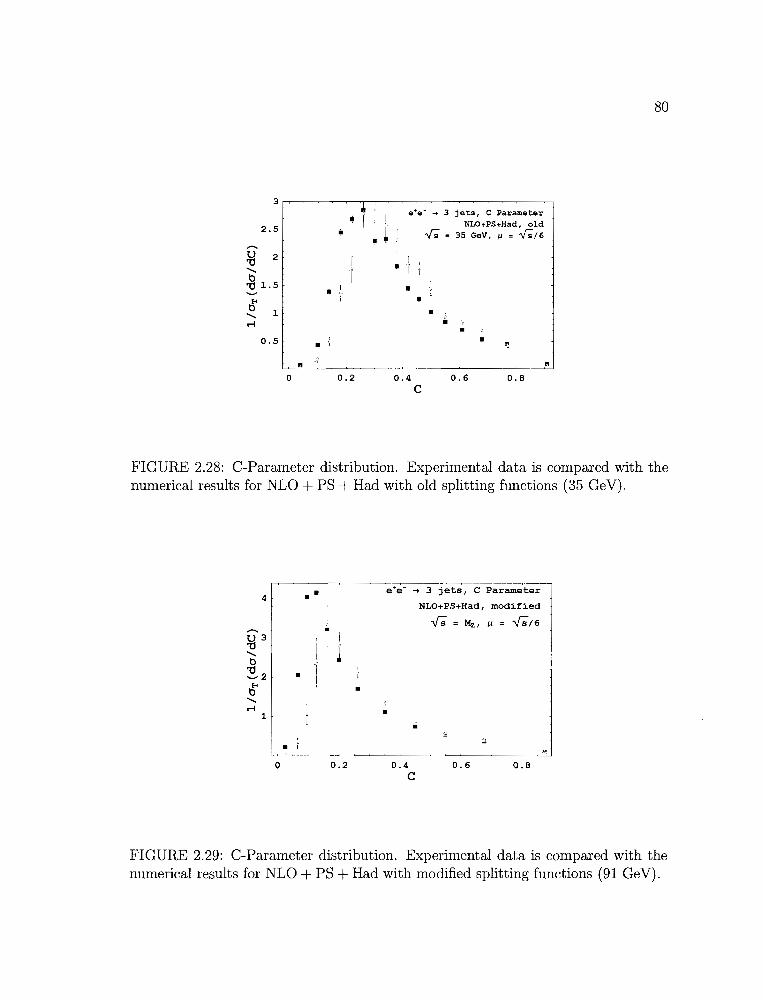
80
3~ eTe- ... 3 jets, C Parameter• I NLO.PS.Had, old2.5 '!' .,f; = 35 GeV, IJ = .,f;/6•......
U 2 I'U....... • I0'U 1.5 • •6' •
....... 1 •..... • •
0.5 • ,.•
" "0 0.2 0.4 0.6 0.8
C
FIGURE 2.28: C-Parameter distribution. Experimental data is compared with thenumerical results for NLO + PS + Had with old splitting functions (35 GeV).
4
1
•
• I
••II
r I~
•
e+e- ~ 3 jets, C Parameter
NLO+PS+Had, modified
ys = Mz , IJ = YS/6
••
o 0.2 0.4C
0.6 0.8
FIGURE 2.29: C-Parameter distribution. Experimental data is compared with thenumerical results for NLO + PS + Had with modified splitting functions (91 GeV).
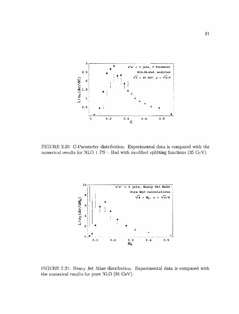
81
2.5
0.5
"o
'"e"e- .. 3 jets, C Parameter
'"'"NLO+PS+Had, modified
I + .y; .y;/6I = 35 GeV, IJ. =
I I• II
• •T
•~ .- ••
..0.2 0.4 0.6 0.8
C
FIGURE 2.30: C-Parameter distribution. Experimental data is compared with thenumerical results for NLO + PS + Had with modified splitting functions (35 GeV).
e+e- .. 3 jets, Heavy Jet Mass
Pure NLO calculations
,r; = Mz , ~ = ,r;/6
•
o l.·0.1
..I
•I
I •
0.2
•..
0.4 0.5
FIGURE 2.31: Heavy Jet Mass distribution. Experimental data is compared withthe numerical results for pure NLO (91 GeV).
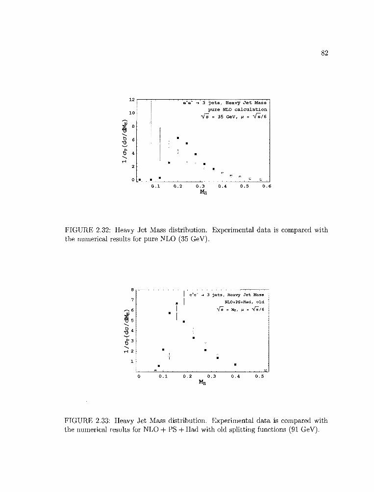
82
••
10
12 ,.----.-~~~~~~~~~~~~~~~~~..,e-e- ~ 3 jets, Heavy Jet Mass
pure NLO calculation
If; = 35 GeV, ~ = If;/6,,-...
~ 8........g 6
f<tl 4
.......rl
2•
••
•o· • •
0.1 0.2 0.4 0.5 0.6
FIGURE 2.32: Heavy Jet Mass distribution. Experimental data is compared withthe numerical results for pure NLO (35 GeV).
••
•
0.5
•0.4
e+e- ~ 3 jets, Heavy Jet Mass
NLO+PS+Had, old
.y;; = Mo, J.l = .y;;/6
0.2 0.3MH
•
•I
• I
•
0.1
•"a
7
1
FIGURE 2.33: Heavy Jet Mass distribution. Experimental data is compared withthe numerical results for NLO + PS + Had with old splitting functions (91 GeV).
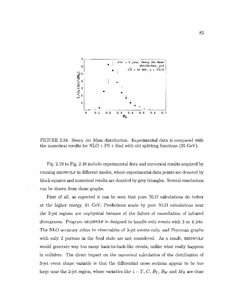
83
I e+e- .... 3 jets, Heavy Jet Mass
• I NLO+PS+Had, old
• ,T,; = 35 GeV, ~ = ,T,;/6
o 0.1 0.2 0.3 0.4 0.5 0.6 0.7MH
FIGURE 2.34: Heavy Jet Mass distribution. Experimental data is compared withthe numerical results for NLO + PS + Had with old splitting functions (35 GeV).
Fig. 2.19 to Fig. 2.48 include experimental data and numerical results acquired by
running BEOWULF in different modes, where experimental data points are denoted by
black squares and numerical results are denoted by grey triangles. Several conclusions
can be drawn from those graphs.
First of all, as expected it can be seen that pure NLO calculations do better
at the higher energy, 91 GeV. Predictions made by pure NLO calculations near
the 2-jet regions are unphysical because of the failure of cancellation of infrared
divergences. Program BEOWULF is designed to handle only events with 3 or 4 jets.
The NLO accuracy refers to observables of 3-jet events only, and Feynman graphs
with only 2 partons in the final state are not considered. As a result, BEOWULF
would generate way too many back-to-back-like events, unlike what really happens
in colliders. The direct impact on the numerical calculation of the distribution of
3-jet event shape variable is that the differential cross sections appear to be too
large near the 2-jet region, where variables like 1 - T, C, BT , Bw and MH are close
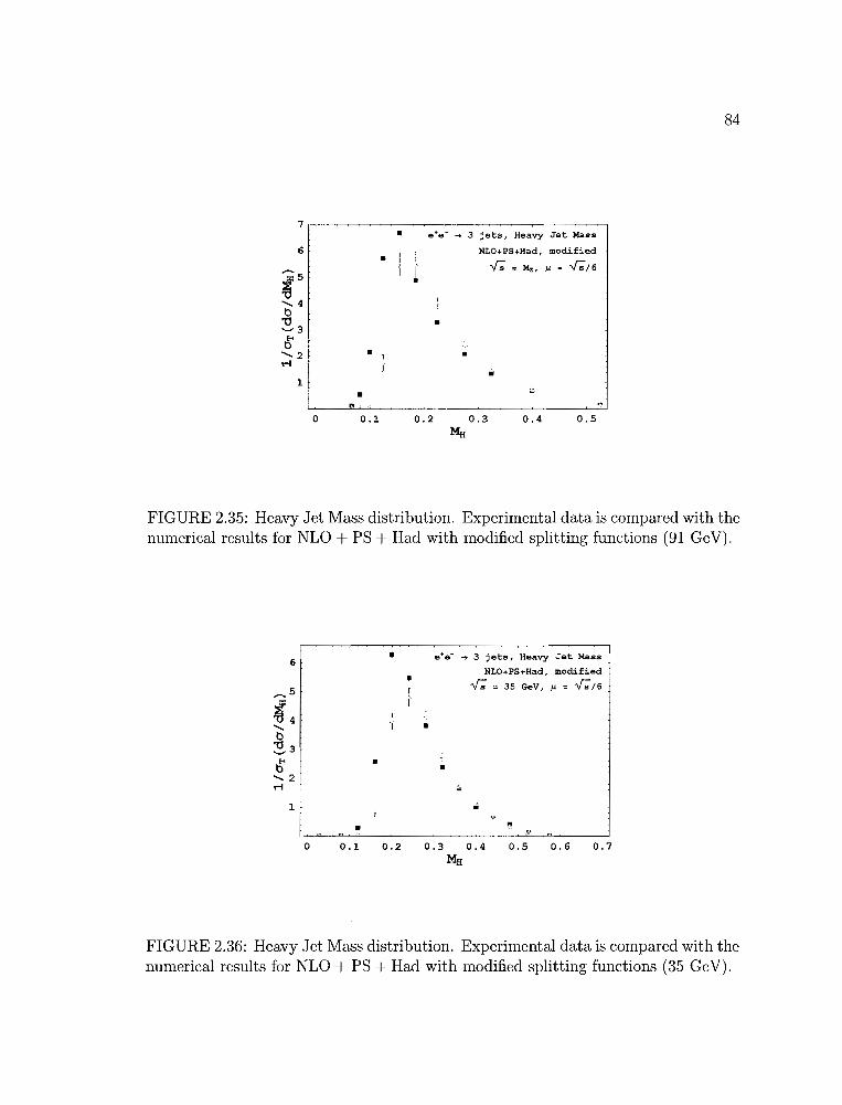
84
6
•
1
•"o 0.1
• e+e- .. 3 jets, Heavy Jet Mass
! I NI.O+PS+Had, modified•
.y; = Mz • .y;/6,~
I' =
•
••
;;;"
0.2 0.3 0.4 0.5MH
FIGURE 2.35: Heavy Jet Mass distribution. Experimental data is compared with thenumerical results for NLO + PS + Had with modified splitting functions (91 GeV).
6
....... 5II:
~4......o~3
6'...... 2.-l
1
•
•
,•
e+e- ~ 3 jets, Heavy Jet Mass
NI.O+PS+Had. modified
.y; = 35 GeV. I' = .y;/6
"o 0.1 0.2 0.3 0.4 0.5 0.6 0.7
MH
FIGURE 2.36: Heavy Jet Mass distribution. Experimental data is compared with thenumerical results for NLO + PS + Had with modified splitting functions (35 GeV).
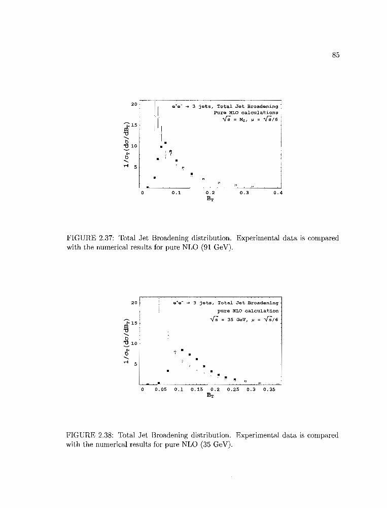
85
20
•
•
• •
e+e- ~ 3 jets, Total Jet BroadeningPure NLO calculations
,(; = Hz, ~ = ,(;/6
..c
•
•
o 0.1 0.3 0.4
FIGURE 2.37: Total Jet Broadening distribution. Experimental data is comparedwith the numerical results for pure NLO (91 GeV).
.. ,.•••
• • •
Q+Q- ~ 3 jets, Total Jet Broadening
pure NLO calculation
,(; = 35 GeV, ~ = ,(;/6
•
"L.-~~.~~~_~~~~~__~~~~----.:.:N,--~
20
o 0.05 0.1 0 . 15 0 . 2 0.25 0 . 3 0 . 35BT
FIGURE 2.38: Total Jet Broadening distribution. Experimental data is comparedwith the numerical results for pure NLO (35 GeV).
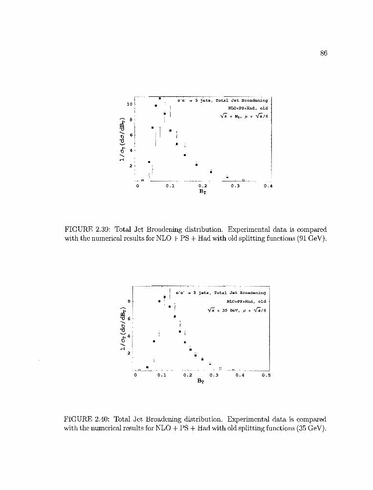
86
••
•
e~e- ~ 3 jets, Total Jet Broadening
NLO+PS+Had, old
...[; = Mz , I' = ...[;/6
0.40.3
•
•
"[ • IE:; a r~ • •b 6"0.......t5' 4
.......r-I •
2
0 0.1
FIGURE 2.39: Total Jet Broadening distribution. Experimental data is comparedwith the numerical results for NLO + PS + Had with old splitting functions (91 GeV).
e·e- ~ 3 jets, Total Jet Broadening
a
•
•• I .[
•
NLO+PS+Had, old
If; = 35 GeV, I' = ...[;/6
••
2 • ••
o 0.1 0.2 0.3 0.4 0.5
FIGURE 2.40: Total Jet Broadening distribution. Experimental data is comparedwith the numerical results for NLO + PS + Had with old splitting functions (35 GeV).

87
•
••
•I• e+e- .... 3 jets, Total Jet Broadening
NLO+PS+Had, modified
IfS = Mz, ~ = 1fS/6
•
•
•
10
....... 8Eo<
~....... 6.g........
6' 4.......r-t
2
o" ,
0.1 0.3 0.4
FIGURE 2.41: Total Jet Broadening distribution. Experimental data is comparedwith the numerical results for NLO + PS + Had with modified splitting functions (91GeV).
to zero. The 3-jet region is far away from those infrared singularities of Feynman
diagrams and pure NLO calculation is supposed to be reliable at energies much
higher than the QCD scale (A '" 1 GeV). However, at low energies, the strong
coupling constant gets bigger, and the perturbation expansions of cross sections will
eventually break down at the QCD scale. Event at energies not as low as A, the
perturbative treatment becomes insufficient to model the important long-distance
effects, such as parton showers and hadronizations, which only happen long time after
the hardest interactions. As foreseen, this discrepancy between pure NLO results and
experimental data in the 3-jet region is much more noticeable at VS = 35 GeV for
almost all event shape variable chosen to be evaluated.
We also made another postulate about the outcome of simulations. Since parton
showers and hadronizations can approximately account for the long distance effects
when the c.m. energy scale is low, we believe the NLO + PS + Had mode of
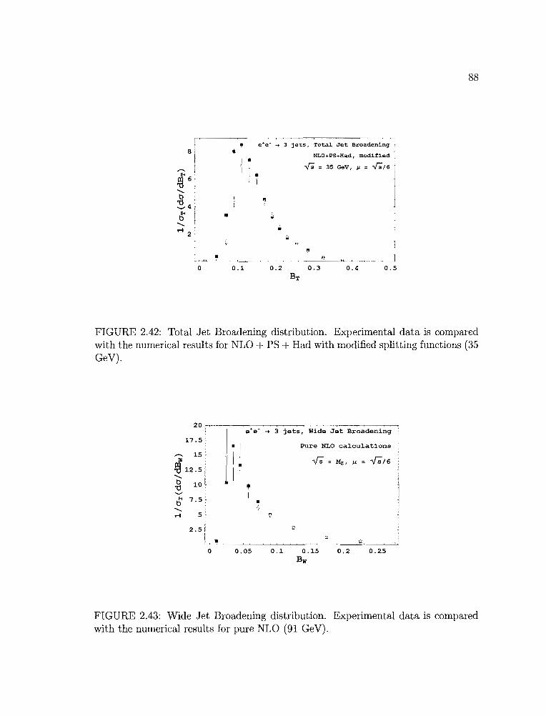
e·e- ~ 3 jets, Total Jet Broadening
NLO+PS+Had, modified
,(,; = 35 GeV, ~ = ,(,;/6
;,[
o•
•
....
0.1
..I, ..I I
0.2
"0.3 0.4 0.5
88
FIGURE 2.42: Total Jet Broadening distribution. Experimental data is comparedwith the numerical results for NLO + PS + Had with modified splitting functions (35GeV).
20
I·e+e- -+ 3 jets, Wide Jet Broadening
17.5 [
IPure NLO calculationsI
....... 15 ~
1i
~ t , -YS= Mz , Ii = -YS/6.rs 12.5 f"
10 lb ..'tl I I6' 7. 5 ~ •" 5 ~.... ~
2. 5 ~ -! :..•
0 0.05 0.1 0.15 0.2 0.25Bioi
FIGURE 2.43: Wide Jet Broadening distribution. Experimental data is comparedwith the numerical results for pure NLO (91 GeV).
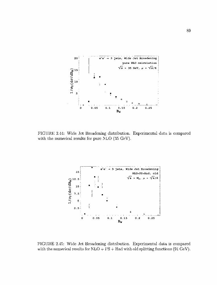
20
~15
f8.......b'U 10......,
6'.......r-l 5
e'e- ~ 3 jets, Wide Jet Broadening
pure NLO calculation
,(; = 35 GeV, ~ = ,(;/6
~ .•
•• ...
• - ..; - '"0 0.05 0.1 0.15 0.2 0.25
Bw
89
FIGURE 2.44: Wide Jet Broadening distribution. Experimental data is comparedwith the numerical results for pure NLO (35 GeV).
• e+e- 3 jets, Wide Jet Broadening j~
15 r NLO+PS+Had, old I[ • I ,(; ,(;/6 j,,-...12.5 [ = Mz , Ii =
IJ: I IJf8 10 ~ • r....... • jb t
'U7.5 t I......, •
,6' r
jj
....... 5 t • jr-li
2.5 f •i
• -0 0.05 0.1 0.15 0.2 0.25
Bw
FIGURE 2.45: Wide Jet Broadening distribution. Experimental data is comparedwith the numerical results for NLO + PS + Had with old splitting functions (91 GeV).
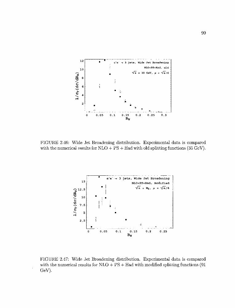
90
12 • • e+e- 3 jets, Wide Jet Broadening..10
NLO+PS+Had, old
.--... • -.r; = 35 GeV, I' = -.r;/6~
~ 8
'"tl'tl 6
Eo< •tl 4
'" •.....•2 ••
" P?
0 0.05 0.1 0.15 0.2 0.25 0.3BW
FIGURE 2.46: Wide Jet Broadening distribution. Experimental data is comparedwith the numerical results for NLO + PS + Had with old splitting functions (35 GeV) .
I •Ii Ij T
•
15
--; 12.5
~ 10
'".g...... 7.5
f;'" 5.....
2.5
•
•
•
• II
e'e- ~ 3 jets, Wide Jet Broadening
NLO+PS+Had, modified
,(; = Mz , I' = ,(;/6
•
o 0.05 0.1 0.15BW
0.2 0.25
FIGURE 2.47: Wide Jet Broadening distribution. Experimental data is comparedwith the numerical results for NLO + PS + Had with modified splitting functions (91GeV).
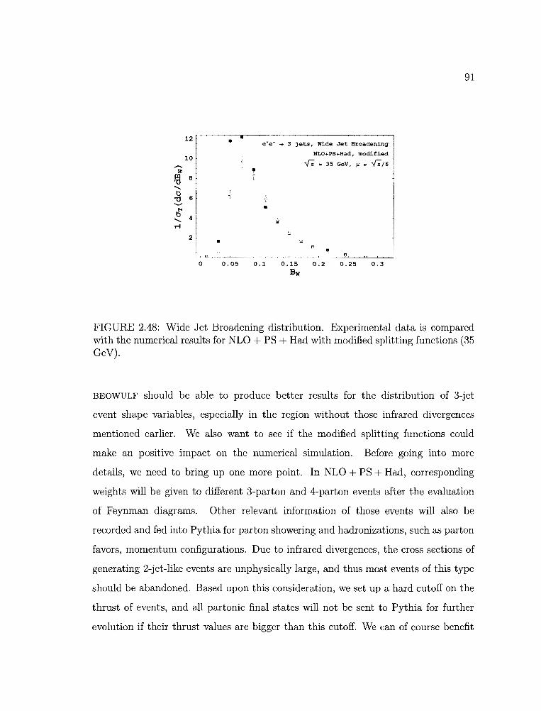
91
•
•
12 ,.-.-~~~,---.-~~~~~~~~~~~~.~e+e- ~ 3 jets, Wide Jet Broadening j
NLO+PS+Had, modified 1
-..[; = 35 GeV, I' = -..[;/6 jI
j
10
2 • .."o 0.05 0.1 0.15 0.2 0.25 0.3
Bw
FIGURE 2.48: Wide Jet Broadening distribution. Experimental data is comparedwith the numerical results for NLO + PS + Had with modified splitting functions (35GeV).
BEOWULF should be able to produce better results for the distribution of 3-jet
event shape variables, especially in the region without those infrared divergences
mentioned earlier. We also want to see if the modified splitting functions could
make an positive impact on the numerical simulation. Before going into more
details, we need to bring up one more point. In NLO + PS + Had, corresponding
weights will be given to different 3-parton and 4-parton events after the evaluation
of Feynman diagrams. Other relevant information of those events will also be
recorded and fed into Pythia for parton showering and hadronizations, such as parton
favors, momentum configurations. Due to infrared divergences, the cross sections of
generating 2-jet-like events are unphysically large, and thus most events of this type
should be abandoned. Based upon this consideration, we set up a hard cutoff on the
thrust of events, and all partonic final states will not be sent to Pythia for further
evolution if their thrust values are bigger than this cutoff. We can of course benefit
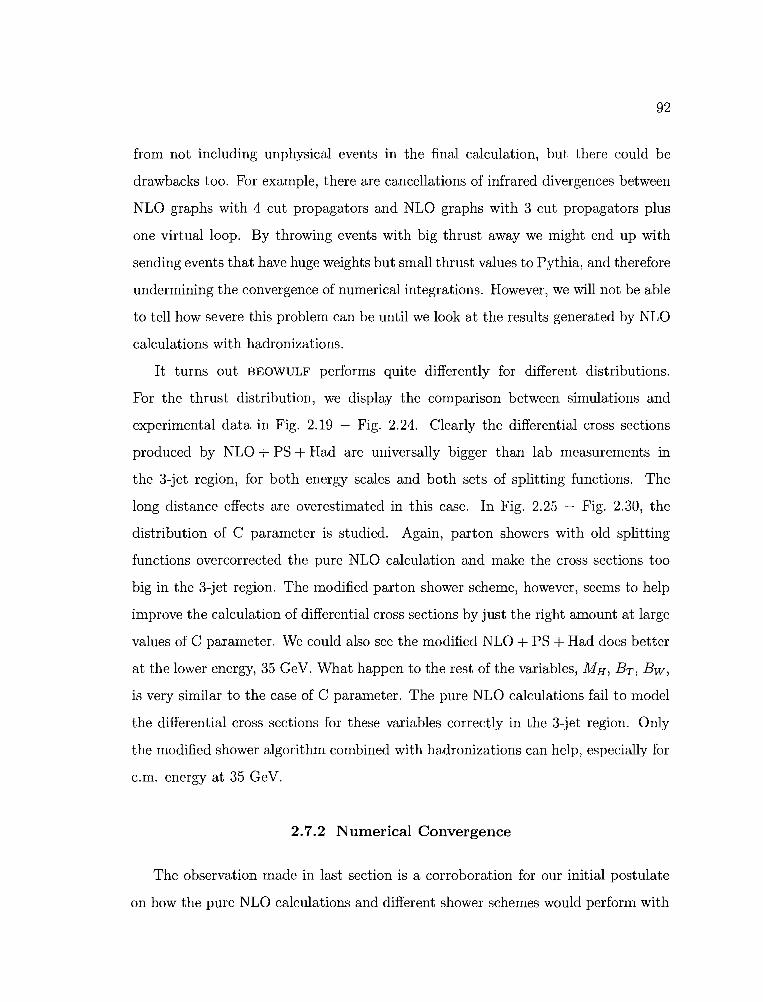
92
from not including unphysical events in the final calculation, but there could be
drawbacks too. For example, there are cancellations of infrared divergences between
NLO graphs with 4 cut propagators and NLO graphs with 3 cut propagators plus
one virtual loop. By throwing events with big thrust away we might end up with
sending events that have huge weights but small thrust values to Pythia, and therefore
undermining the convergence of numerical integrations. However, we will not be able
to tell how severe this problem can be until we look at the results generated by NLO
calculations with hadronizations.
It turns out BEOWULF performs quite differently for different distributions.
For the thrust distribution, we display the comparison between simulations and
experimental data in Fig. 2.19 - Fig. 2.24. Clearly the differential cross sections
produced by NLO + PS + Had are universally bigger than lab measurements in
the 3-jet region, for both energy scales and both sets of splitting functions. The
long distance effects are overestimated in this case. In Fig. 2.25 - Fig. 2.30, the
distribution of C parameter is studied. Again, parton showers with old splitting
functions overcorrected the pure NLO calculation and make the cross sections too
big in the 3-jet region. The modified parton shower scheme, however, seems to help
improve the calculation of differential cross sections by just the right amount at large
values of C parameter. We could also see the modified NLO + PS + Had does better
at the lower energy, 35 GeV. What happen to the rest of the variables, MH , BT , Bw ,
is very similar to the case of C parameter. The pure NLO calculations fail to model
the differential cross sections for these variables correctly in the 3-jet region. Only
the modified shower algorithm combined with hadronizations can help, especially for
c.m. energy at 35 GeV.
2.7.2 Numerical Convergence
The observation made in last section is a corroboration for our initial postulate
on how the pure NLO calculations and different shower schemes would perform with
93
respect to the evaluation of 3-jet event shape variable distributions. However, as
discussed earlier, we still need to examine the convergence of numerical integrations.
In other words, the systematic and statistical errors of the numerical results have to
be studied before we can make use of any of those to extract useful information, eg.,
the strong coupling constant as.
Program BEOWULF has a built-in mechanism to check the convergence of the
numerical integrations. Let us take an example the calculation of C parameter of
generated events. Roughly speaking, this observable are calculated in BEOWULF
by taking the sample mean of the C parameter values of all N events. The C
parameter value of each individual event is of course supposed to be a random number,
and can be affected by many different factors. The events are generated randomly
according to a pre-determined distribution, and therefore the C parameter values of
N events should be independent and identically distributed. On the other hand, the
sample mean of the C parameter values is also a random variable. Central Limit
Theorem (CLT) says the sample mean of those C parameters will approach a normal
distribution when the sample size N - 00, as long as the distribution of individual
C parameter value has a finite mean and variance. As a result, we can examine the
distribution of the sample mean and draw conclusions about the convergence of the
underlying distribution of the C parameter.
To better illustrate what can be done to study the distribution of sample mean, let
us consider a random variable X. Generate N samples of X independently according
to the same distribution. We call the value of the ith sample Xi. The central moments
/-Lr of this distribution is defined as
where /-L without any index is the expectation value of the random variable,
/-L == (x) .
(2.150)
(2.151)

94
The second central moment f.L2 is also called the variance. In a normal distribution
P(x) = _1_e-(x-J.l)2/(2172
) , (2.152)(5V2i
it can be easily proved that the mean of the variable X is f.L and the variance is (52.
The first and the third central moments of any normal distribution are zero. The
second central moment f.L2 by definition is just (52, and the fourth central moment is
(2.153)
So, if people want to prove an unknown distribution is normally distributed, they
can first calculate both the second and fourth central moment, and see if
(2.154)
IS satisfied. The problem is, with finite number of samples we do not know
what f.L is for this distribution, and further more there is no way to calculate the
expectation values of powers of (x - f.L). However, one can always construct unbiased
estimators for the second and fourth central moments, and see if the estimators
could approximately satisfy Eq. (2.154) when the sample size is large. The reason is
according to the Law of Large Numbers, the unbiased estimator of any expectation
value should converge to the same expectation value when the sample size increases
to infinity.
In our case, the objective is to investigate the distribution of the sample mean of
an underlying variable X,
(2.155)
We call this new random variable X. In order to construct unbiased estimators of
the second and the fourth central moments of X, one needs to find out the relations
between the central moments of X and those of X, and then calculate the estimators
95
for the distribution of X. Any direct calculation of the unbiased estimators for the
central moments of X would be practically very unreliable, because usually it takes
hours to generate just one sample of X, and the estimators will not converge with
very few samples. Meanwhile, it only takes "-' 1 micro second to produce a sample
of the variable X. Notice that (Xl = (X) = J..l. By making use of tools such as the
characteristic functions of probability distributions, one can derive the following:
J..l2 (X)
J..l4 (X)
11,2 (X)N
3 (2N - 3) J..l2 (X)2 + (N2 - 3N + 3) J..l4 (X)N3 (N - 1)
(2.156)
(2.157)
If we denote the power sum of variable X with
and define
(2.158)
(2.159)
(2.160)
N~l (-~~+~)1 (35t 65i52 45153 54)
(N - 1)2 - N4 + ----y:j3 -~ + N
One can show that the expectation values of m2 and m4 are equal to the second
and the fourth central moment of the distribution of the sample mean of X. As
pointed out earlier, this same distribution will approach a normal distribution if the
underlying variable X has finite mean and variance. On the other hand, calculating
the sample mean of X is in principle equivalent to integrating X over all possible
parameter space. This integral converges well is only another way of saying it has
finite mean and variance. Therefore, if we find out the following is true when the
sample size N is large,
(2.161)
96
we would be able to conclude the corresponding integration must have converged well.
This is precisely what BEOWULF does to test the convergence of variance numerical
integrations, including the calculation of differential cross sections in bins of different
event shape variables. For every integral of variable X there is a sample mean X,
and a pair of unbiased estimator for the second and the fourth central moments of
X. One can be alarmed by a pair of m2 and m4 that cannot even remotely satisfy
Eq. (2.161) if there is something wrong with the cancellation of divergences. When
calculating those event shape variables whose distributions are plotted somewhere
between Fig. 2.19 and Fig. 2.48, we observe that from time to time m4 is twice or
three times bigger than m2.
The marginal convergence of some differential cross sections is inherent with the
way we treat Feynman graphs in BEOWULF. At leading order, only events with
3 partons are included and further showered. However, the LO graph with 3 cut
propagators becomes divergent when two of them that come out of the same uncut
propagator become collinear with each other. It means events with large thrust
and 3 partons will be generated at an unphysically high rate, or equally, generated
with unphysically large and positive weights. There would not be any problem if
all Feynman diagrams are included, because events from the LO graph with only
two cut propagators and one virtual loop can have large and negative weights, and
hence eliminate the divergence when the total cross section of e+e- -----* hadrons is
calculated. However, events of the second type are ignored and discarded, because
BEOWULF is designed to deal with events with 3 hard partons or more. Points
of finite values in the Monte Carlo integration with huge and unbalanced weights
are equivalent to points with large values. As a result, after primary splittings,
BEOWULF will produce many events with large and positive weights near the two
jet region, and we have to make a hard cut-off on the thrust values of events. The
motive is to get rid of those unphysical events and have finite total cross section
when normalizing the differential cross sections. However, many events of this type
97
with thrust values slightly smaller than the cut-off would still be sent to PYTHIA.
After further showering and hadronization in PYTHIA, a portion of those events can
get broadened, and their values of event shape variables could be comparable to
those real 3-jet events. These events that have very large thrust values before parton
showering possess unbalanced positive weights, and hence will make the differential
cross sections higher than what they should be in the 3-jet region. For interactions at
.JS = 91 GeV, the long-distance effects are weaker than those at .JS = 35 GeV, and
as we see, parton showers overshoot and make the simulation results deviate further
away from the experimental data in the 3-jet region.

,98
CHAPTER III
COLORFUL QUANTUM BLACK HOLES
3.1 Introduction
The Standard Model of particle physics is perhaps the most successful physics
theory up until now. It unifies the Maxwell's theory of electromagnetism and the
Weak Interaction, describes the strong interaction as a non-Abelian gauge field, and
yields many theoretical predictions that have been matched with experimental data
to very impressive accuracy. As a very powerful field theory, Standard Model has
its own limitations. The theory has too many input parameters to be adjusted.
In addition, the mechanism responsible for breaking the electroweak symmetry and
generating particle masses in this model is not yet fully understood. The mass of
neutrinos cannot be explained; Higgs boson mass, which is only of order 102 GeV,
receives quantum corrections that are sensitive to the cut-off scale ('" 1019 GeV),
and thus seems to be radiative unstable. The Large Hadron Co1lider (LHC) has been
built to help physicists tackle those problems, which is able to constantly smash
proton-proton beams at a c.m. energy v's = 14 TeV. At this scale, we should be
able to reveal the real scheme that breaks the electroweak symmetry, and as a result,
solve the hierarchy problem.
There have already been various candidates that could stabilize the hierarchy
mEW/Mpl, such as Supersymmetry and Extra Dimensions. Our project is to explore
one bold and yet possible outcome, the production of quantum black holes at
the LHC, assumIng there are indeed compactified extra dimensions in addition to
ordinary 4-dimensional spacetime. It will be explained how we attempt to constrain
99
the decay of black holes created in a proton collider. However, it would be worthwhile
to first say a bit more about the origin of extra dimension scenarios, the reason behind
their revival, and how they give rise to the possibility of producing micro black holes.
3.2 Extra Dimensions
3.2.1 Kaluza-Klein Theory
In the early 20th century, people discovered that five-dimensional spacetime can
be splitted into the Einstein equations and Maxwell equations in four dimensions,
which was an attempt to unify gravity and electromagnetism. Oscar Klein later
suggested the fifth dimension can be curled up in a extremely small circle, so that
a particle will come to its original position very shortly if it travels along this
extra dimension. The distance a particle can move before returning to where it
started is defined as the size of the extra dimension. People call extra dimensions
of this type a compact set, and call the phenomenon of a spacetime having compact
extra dimensions compactijication. From an experimentalist's view, the compact fifth
dimension can be tested. Standing waves should be allowed to exist, and have an
energy spectrum
En = nhc/R, (3.1)
where R is the size of the extra dimension, h is the Planck's constant, c is the speed of
light and n is a positive integer. This set of energies corresponds to the mass spectrum
of a set of resonance, and we call this spectrum the K aluza-Klein Tower. In particle
reactions those standing waves can in principle be produced through resonance, and
can at the same time be identified in the particle detectors as missing energies that
could fill in the Kaluza-Klein Tower.
(3.2)
100
Kaluza-Klein theory has a very elegant geometric presentation, but it was
forgotten not long after it was first invented, because it ran into a series of problems
and was not able to be converted to a realistic model. For example, fermions must be
introduced in an artificial way in the Kaluza-Klein theory, unlike the modern standard
model where fermions obey various gauge symmetries and have to be sorted in a
specific fashion. The existence of new generations of fermions can even be predicted
in order to explain CP violation within the framework of standard model. It would be
great if the standard model of particle theory could be embedded into the beautiful
geometry of Kaluza-Klein theory.
3.2.2 The Hierarchy Problem
In standard model, the hierarchy between the electroweak scale mEW and an
ultraviolet cut-off scale Auv is large, because Auv is usually considered to be the
Planck scale,
M D- 2 = (27f)D-4PI - ,47fGVD - 4
where D is the dimension of spacetime, G is the Newton's constant, and VD - 4 is
the volume of the compact space. As a result, the Higgs boson mass is radiatively
unstable, since it receives quadratically divergent quantum corrections through
the coupling between ordinary fermions and the Higgs boson. In supersymmetric
models, super partners of standard model particles are proposed to stabilize the
hierarchy problem. For every standard model fermion, there is a scalar particle
as its super partner. Those scalars are coupled to the Higgs boson in a way such
that the corresponding corrections to the Higgs boson mass will exactly cancel the
corrections induced by virtual standard model fermions. However, supersymmetry is
not apparent based upon existing experimental data, and thus the mechanism that
breaks supersymmetry needs to be studied.
101
Compared to the approach of supersymmetry, the solution to the hierarchy
problem in extra-dimensional theories seems trivial. In such theories, there is only
one fundamental scale, instead of two. The standard model theory is only valid up to
the electroweak scale. Gravitational effects will become important beyond that scale,
and the ordinary 5U(3) x 5U(2) x 5U(I) field theory will break down. Simply by
construction there is no such thing as severe hierarchy between the electroweak scale
and the ultraviolet cutoff scale. In fact, whether the hierarchy problem can really be
resolved in such a straightforward way depends on if one can lower the Planck scale
to the Tera electron volt (TeV) scale.
It is worthwhile to define the Planck scale first. In quantum mechanics, the
smallest scale of localizing a particle is this same particle's Compton's wavelength.
Compton's wavelength of a particle is equivalent to the wavelength of a photon whose
energy is equal to the rest mass m of that particle,
hAc =-.
me(3.3)
According to the Heisenberg Uncertainty Principle, if we use a light of certain
wavelength to measure the position of some particle, the momentum and the position
of that particle obeys the following:
b.x . b.p > 11,/2 ,
which can be also written down as a lower limit for b.p:
11,b.p> ~.
2ux
(3.4)
(3.5)
The uncertainty in particle momentum can not be infinitely large, either. Because as
soon as b.p > mc, the energy of the particle would become greater than the threshold
of creating a new particle of the same type, which is equal to the rest mass mc2, and
the measurement of the position of the original particle would be undermined. In

102
quantum field theory this argument is qualitively justified, and photons can indeed
create a pair of fermions as long as the photon energy is larger than the rest mass of
the two fermions. After we put this constraint for ~p in Eq. (3.5), immediately we
will have
n~x>-
2mc'(3.6)
which is equivalent to saying the smallest length scale a particle can be localized
is its Compton's wavelength, up to a factor of order 1. On the other hand, let us
consider a black hole of mass MBH . Assume this black hole is not rotating and
spherically symmetric for simplicity. All the massive material is trapped behind its
event horizon, which is a spherical surface of radius equal to the SchwarzschiId radius
(3.7)
where G is the Newton's gravitational constant. However, the size of the black
hole can not be smaller than its own Compton's wavelength, otherwise the quantum
fluctuation of the massive material that forms the black hole will overrule the
gravitational effects, and the black hole will disappear instantly as the massive
material can no longer be trapped behind the event horizon. Combined with Eq. (3.7),
this argument leads to
(3.8)
up to a factor of order 1. This smallest mass of a black hole is defined as the Planck
mass, M pl , and the Planck scale, rv 1019 GeV, corresponds to the Planck mass by
the mass-energy equivalence.
In extra-dimensional models, the Planck scale can be much lower than 1019 GeV
if the size of the extra dimensions is large. A well-accepted argument that supports
this claim is given in [21] by Arkani-Hamed, Dimopoulos and Dvali in 1998. Assume
103
a model with 4 ordinary spacetime dimensions and n compactified extra dimensions.
Intuitively speaking, the gravitational field can be diluted by the n extra dimensions.
It is possible that at TeV scale the gravity has already become as important as the
gauge forces if we take all dimensions into account. Suppose the standard model
fields can only propagate in the ordinary 3 spatial dimensions but gravitational field
can freely propagate in all spatial dimensions, then the gravitational field would still
look much weaker than the other forces in the ordinary 3 spatial dimensions. It
means the Planck scale that is induced from measuring the effective gravitational
coupling GN in the ordinary 3 spatial dimensions could be much higher than what
the real Planck scale should be.
Let us perform a rough quantitative analysis (see [21] for more details). The
Planck scale M pl = G1.//2 if we adopt the system of units in which n= c = 1. The
Gauss's law is approximately right with 3 spatial dimensions, and the gravitational
potential between object of mass ml and another object of mass m2 is
(3.9)
V (r) Gmlm2
N-r
mlm2 1M~l -;;.
If there are n compactified extra dimensions of size R, for length scale far smaller
than R, the n extra dimensions would not be very different from the ordinary 3
spatial dimensions. The Gauss's law should be modified accordingly by first putting
in a new factor of l/rn, because the Gaussian sphere now has n more dimensions.
The gravitational potential should remain linear with the masses of individual field
sources. Using dimensional analysis, there should also be a new factor of 1/Mpl , and
hence we have
h M 2+nwere PI(4+n)
mlm2 1V (r) rv M 2+n n+l' (r «R) ,
PI(4+n) r
is the true Planck scale in 4 + n dimensions.
(3.10)
In comparison, at a
104
distance ~cale much larger than R, the compactified dimensions are almost invisible,
and the Gauss's law for gravitational potential should have the same r dependence as
that in Eq. (3.9). Matching the two different expressions for gravitational potential
at the boundary r = R, one can derive the following for r » R:
mlm2 1V (r) rv M 2+n Rn ,(r» R) , (3.11)
PI(4+n) r
and thus the effective Planck scale Mpl in 4D spacetime can be expressed in terms
of MPI (4+n)' The relation between the effective scale and the true scale is simply
M 2 M2+n RnPI = PI(4+n) . (3.12)
If we let MPI (4+n) be of order 103 GeV, which is the scale of mEW, the hierarchy
problem can be solved naturally. We also want to push the effective Planck scale
(Mpl ) up to the measured value (rv 1019 GeV), and as a result one would derive
(
3 ) l+~R rv 1O~-17cm x 10 GeV n, (3.13)mEW
where n is the number of extra compactified dimensions. From here we will use MD
instead of MPI(4+n) to denote the Planck scale in 4 + n dimensions. Notice that R
has be smaller than the smallest length scale (rv 1 cm) at which Newton's law of
gravity can be tested in any available experiments, otherwise we would have already
observed deviations. The case of n = 1 has been ruled out because it corresponds to
R rv 1013 cm. For scenarios with n 2:: 2, the size of the compactified dimensions would
be smaller than 1 mm, and thus they are still in play. It is well motivated to question
the validity of Newtonian gravity at distance smaller than 1 cm. The present Planck
scale is only extrapolated from current measurements, and it corresponds to 10-33
cm. Believing the real Planck scale to be rv 1018 GeV is no different from believing
nothing happens to the gravity between the above two widely separated scales.
The Kaluza-Klein theory has been revived in this way, with many new elements
added in. People have invented theoretical techniques to prevent standard model

105
fields from leaking into the compactified dimensions, and therefore the modern
versions of extra dimension theories can possess realistic particle contents that were
missing from the original theory. One of the most well-known extra-dimensional
scenarios that encompass the standard model is ADD[21], and another one is the
Randall-Sundrum (RS) model [22]. We will adopt these two scenarios when we
investigate quantum black holes later.
3.3 Black Hole Formation at the LHC
An important consequence of using extra dimensional models to explain hierarchy
problem is that black holes may be able to form at a much lower scale than what
people thought. If the Planck scale were to be proved to be actually close to 1 TeV,
black holes with masses greater than 1 TeV can exist despite quantum fluctuations.
People even suggest black holes can be produced colliding proton pairs at the Large
Hadron Collider (LHC) which runs at a c.m. energy of 14 TeV, based on the hoop
conjecture. The hoop conjecture was first proposed by Kip Thorn[23] in 1972, and
states:
A n imploding object forms a black hole when, and only when, a circularhoop with a specific critical circumference could be placed around the objectand rotated . .. , and the critical circumference is given by 2 times 1T timesthe Schwarzschild radius corresponding to the object's mass.
According to the hoop conjecture, as long as the impact parameter b is larger than 2
times the Schwarzschild radius corresponding to the mass of the two colliding protons
at the LHC, a small black hole would be formed. This is illustrated in Fig. 3.1.
Black holes of astrophysical size are supposed to evaporate into all available fields
through Hawking radiation. Typical Hawking radiation of such a macroscopic black
hole is believed to be democratic in a sense that the particle production rates are
independent of their flavors. It is very different from any Standard Model decay
process where gauge symmetries put tight constraints on what the final states can
be.
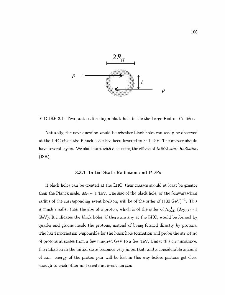
106
pb
p
FIGURE 3.1: Two protons forming a black hole inside the Large Hadron Collider.
Naturally, the next question would be whether black holes can really be observed
at the LHC given the Planck scale has been lowered to rv 1 TeV. The answer should
have several layers. We shall start with discussing the effects of Initial-state Radiation
(ISR).
3.3.1 Initial-State Radiation and PDFs
If black holes can be created at the LHC, their masses should at least be greater
than the Planck scale, MD rv 1 TeV. The size of the black hole, or the Schwarzschild
radius of the corresponding event horizon, will be of the order of (100 GeV)-l. This
is much smaller than the size of a proton, which is of the order of AQ~D (AQCD rv 1
GeV). It indicates the black holes, if there are any at the LHC, would be formed by
quarks and gluons inside the protons, instead of being formed directly by protons.
The hard interaction responsible for the black hole formation will probe the structure
of protons at scales from a few hundred GeV to a few TeV. Under this circumstance,
the radiation in the initial state becomes very important, and a considerable amount
of c.m. energy of the proton pair will be lost in this way before partons get close
enough to each other and create an event horizon.
107
In QeD, the effects of IR are incorporated into the DGLAP evolution of parton
distribution functions (PDF) as the scale of the eventual transverse interaction varies.
An example is the parton distribution function for an up quark inside a proton,
fu (x, Q), which expresses the probability the proton probed at scale Q contains an
up quark of longitudinal momentum fraction x. Since the black holes are believed
to be created at the parton level, the particle level cross section will have to be the
parton level cross section convoluted with the PDFs. To address this issue more
clearly, let us first define the momentum fractions of the two incoming partons to
be X a and Xb. If the c.m. energy of the initial proton pair is vIS, then the energy
actually available for producing the energy would be
(3.14)
where the new parameter u is defined. Taking both general relativity and quantum
fluctuations into account, we should have the threshold s 2: Mb. The full particle
level cross section (T can then be calculated as the following:
(Tpp-.BH+X (s)
(3.15)
where aab-.BH (M~H = s) is the parton level cross section of creating a black hole
of mass MBH , and we will discuss this cross section later. Both a and b are the
parton types in the two initial protons, and the sum run over all possible pairings of
quarks and gluons. The scale Q at which PDFs are evaluated is determined by the
inverse length scale of the interaction. For perturbative hard scattering in a local
field theory, this momentum scale is the momentum transfer, and in an s-channel
reaction it is just the c.m. energy Q "-' .J§. For a non-perturbative s-channel process
in the black hole formation of classic general relativity, it makes sense to take the
size of the horizon as the relevant scale, and Q "-' r;l [24]. Apparently there are two
108
competing effects when producing a black hole in this way. Intuitively, the parton
level cross section of black hole production should become larger as the black hole
mass increases, because the corresponding Schwarzschild radius gets bigger as more
energy is trapped behind the event horizon. On the other hand, the PDFs fall rather
rapidly at high energies as any single parton demands more energy from its mother
proton, due to more severe energy loss through initial-state radiation. It turns out,
without giving any proof here, the effects of the drop of PDFs dominates, and the
consequence is most of the black holes will be created at the threshold, with the c.m.
energy of the proton system fixed.
We can write the particle cross section above in a more convenient form for later
use. Make a variable change by replacing Xa and Xb with u and v. As defined earlier,
u == XaXb. Let v == Xb. Straight forwardly, we will have
(J'pp->BH+X (s) t t dvJ!!b du Ju ---;; "Lfa(u/v,Q)fb(V,Q)'
s a,b
. Crab->BH (M~H = s) .
3.3.2 Inelasticity
(3.16)
In the previous section, we have naively taken the mass trapped the event horizon
to be equivalent with the parton c.m. energy.j§. This is a poor approximation,
considering the fact a great non-negligible portion of .j§ will escape in gravitational
waves even at impact parameter b = O. We have not specified any form for the parton
level cross section of black hole formation, either. We will discuss this particular cross
section in the current section, which will account for the inelasticity inherent in the
grazing collisions of high energy particles.
Based upon the hoop conjecture, naively one would suggest using the geometric
cross section
109
(3.17)
as the parton level cross section. However, the shape of the horizon would not be
a perfect circle as a result of a grazing collision, and therefore Eq. (3.17) would not
be accurate enough for computational purposes. Yoshino and Nambu [25] quantified
the inelasticity y == MBH / Y§ using a system originally set up by D'Eath and Payne
[26], and derived lower bounds on y, as a function of the number of extra dimensions
n and the impact parameter b. Qualitively an inelasticity y < 1 means there is even
less energy available for producing a black hole, and the chance of finding a black hole
with mass much greater than the threshold is even more slim. Another implication
is that the parton level cross sections should be weighted by their impact parameters
when calculating the particle level cross sections. If modifying Eq. (3.16) accordingly,
one can get the following:
{}pp-+BH+X (8, n, MD ) 11 hIlIdv2zdz M2 du -F(n)7rr;(U8,n,MD )·o ~ u V
y s
.L fa (u/v, Q) fb (v, Q) , (3.18)a,b
where z = b/bmax , and F (n) is the form factor that accounts for the deviation of the
shape of the horizon from a perfect sphere. We use the numerical values provided in
[25]. In addition, rs is the Schwarzschild radius of the horizon in (4 + n) dimensions.
The exact definition of r s depends on the normalization convention for the Planck
scale, and we will use the following,
where
k(n) == [2np_3 r[(n+3)/2]]1/(n+l) .n+2
(3.19)
(3.20)
110
Although the numerical lower bounds for the inelasticity y is used in Eq. (3.18), one
should keep it in mind that the particle level cross sections calculated in this way
are only rough estimates. A real calculation involving the grazing collision of high
energy particles should take effects of true quantum gravity into account, since we
are indeed discussing the black holes near the threshold.
3.3.3 Semi-Classic Black Holes
People have been studying black holes of astrophysical size for years using general
relativity. For a black hole that might potentially be produced during a proton
proton collision, there must be important quantum effects involved. The best way
to tell whether a black hole has been produced in the collider is to look for its decay
produces, and people can only attempt to make predictions for the decay of such
black holes using semi-classical analysis in the absence of a theory of real quantum
gravity. Obviously, several criterions have to be satisfied in order to justify this kind
of approach, and any black hole that meets the criterion given next would be a truly
thermal black hole.
Most people would agree that a black hole can be produced if the c.m. energy of
the system E is much larger than the higher-dimensional Planck scale MD. It remains
to be ambiguous at which exact scale a black hole could be formed. Planck scale is
only a lower limit of the real threshold of black hole creation. For this purpose,
we use a parameter, Xmin, to describe the relation between the threshold and the
fundamental scale of gravity, and
Xmin == MminBR/MD. (3.21)
where MminBR is the mass of a black hole at the threshold.
Black holes that are often studied are a derivative of the Einstein's theory of
gravity, and they are usually thermalized, which means those black holes can reach
an internal thermal equilibrium. Let us get a sense of what Xmin could be if all

111
possible black holes have to be thermalized. More detailed analysis can be found in
[271. For such a black hole, the initial entropy So of course has to be large enough to
ensure a well-define thermodynamic description [28]. More specifically, the following
needs to be satisfied:
(3.22)
which is another way of requiring the change in the Hawking temperature is small
per particle emission. This particular criterion yields Xmin f"V 1 for both ADD and
RS. A similar but stronger constraint could come from restricting the energy carried
by any individual degree of freedon in a thermal bath to be much smaller than the
total energy:
(3.23)
This second criterion can be satisfied in both ADD and RS if Xmin :::: 2 [27].
In addition, the life time T of a semi-classical black hole should be large compared
to its inverse mass, Mi3J.r, so that the black hole can behave as a well-defined resonance
[29]. It is found in [27] that this criterion is satisfied for Xmin f"V 1.3 in ADD and for
Xmin f"V 1.6 in RS.
Another possible constraint on the mass threshold for thermal black holes comes
from a concern on the set up of the extra-dimensional model. The black hole
mass should be large compared to the 3-brane tension so that the brane does not
significantly perturb the black hole's metric [29]. The value of an appropriate Xmin
largely depends how exactly the standard model is localized in the ordinary 4D
spacetime, and thus in this article we will not use this criterion to put limits on Xmin.
Furthermore, when a truly thermal black hole decays on the brane, it should be
able to re-equilibrate itself as it decays [27]. It qualitively means the lifetime of the
black hole should be greater than the radius of the event horizon. In ADD, it is
(3.24)
112
necessary to let Xmin 2': 3 in order to satisfy this condition, while any values of Xmin
works well in RS.
Based on the above analysis, it is straight forward to conclude that Xmin ~ 3 is
favored as the ratio of the minimum thermal black hole mass to the Planck scale,
under the normalization convention for the Planck scale we adopted. As discussed
earlier, most black holes will be generated near the threshold, if we also take into
account the drop of PDFs at high energies and the inelasticity of grazing collisions.
A Xmin ~ 3 says the semi-classical black hole production rate would be far less than
the rate with the threshold to be simply the Planck scale itself. This argument will
be confirmed in our numerical results presented later in this article. For now we only
want to stress the fact that most events involving strong gravitational effects might
not even be able to be separated from the Standard Model background, because their
decay products would probably lack the dramatic characteristics of the final state of
a typical thermal black hole.
It is worthwhile to investigate proton reactions with energies greater than the
Planck scale but smaller than the threshold of creating thermal black holes. Before
that, it is helpful to figure out the average number of particles an ordinary black hole
could emit. One can extrapolate from such semi-classical analysis and get a sense of
what those "intermediate" "bound states" would look like. During a typical Hawking
radiation, a black hole would lose its mass through emitting particles. The Hawking
temperature of such a black hole can be related to its Schwarzschild radius in the
following way:
1
r = 1+ n = k (n) ( M ) l+n
4nTBH M D M D 1
where n is the number of compactified dimensions. Not surprisingly, the Hawking
temperature plays a significant role in determining the properties of black hole decay.
The average emission rate for various particle species from a black hole, or the
change in the average multiplicity (N), can be expressed in terms of the Hawking
113
temperature. The change in the black hole's mass can also be related to the Hawking
temperature, radius and some other relevant quantities. Without much difficulty, one
can combine the two above rates together and derive the average multiplicity (N) in
terms of the mass of the same black hole, so that we would get an idea of roughly
how many particles can be found after the decay. After the dust has settled, we have
[29]
2+n
(N) = 4-rrpk (n) [MBH ] I+n = 52+n MD Po,
where 50 is the initial entropy of the black hole,
(3.25)
00= (l+n) MBH .Vi 2 + n T
BH(3.26)
It makes sense that we can derive a relation where the multiplicity of the black hole
is proportional to its entropy, since the entropy of an arbitrary object is in principle
a measure of the number of its possible microscopic configurations. The function
k (n) has been defined in Eq. (3.20). For function p, we only need to know it is
determined by the Hawking temperature, the internal degrees of freedom of different
particle species, and the statistical properties of all available particles that can be
emitted. It accounts for the backscattering of part of the outgoing radiation into the
black hole. In [29], P is calculated to estimate the average multiplicity. It is found
that (N) ;:::j 0.30MBH /TBH , which is about a factor of 3 times smaller than the initial
entropy.
We can assume the semi-classcal black holes with thermally distributed final state
particles obey Poisson distribution. Then (N) becomes the expectation value of the
Poisson distribution. Based upon the above assumption, we can roughly compare
the relative abundances between low-multiplicity events and high-multiplicity events
by simply using
p. _ -(N) (N)i• - e .,'
~.
(3.27)
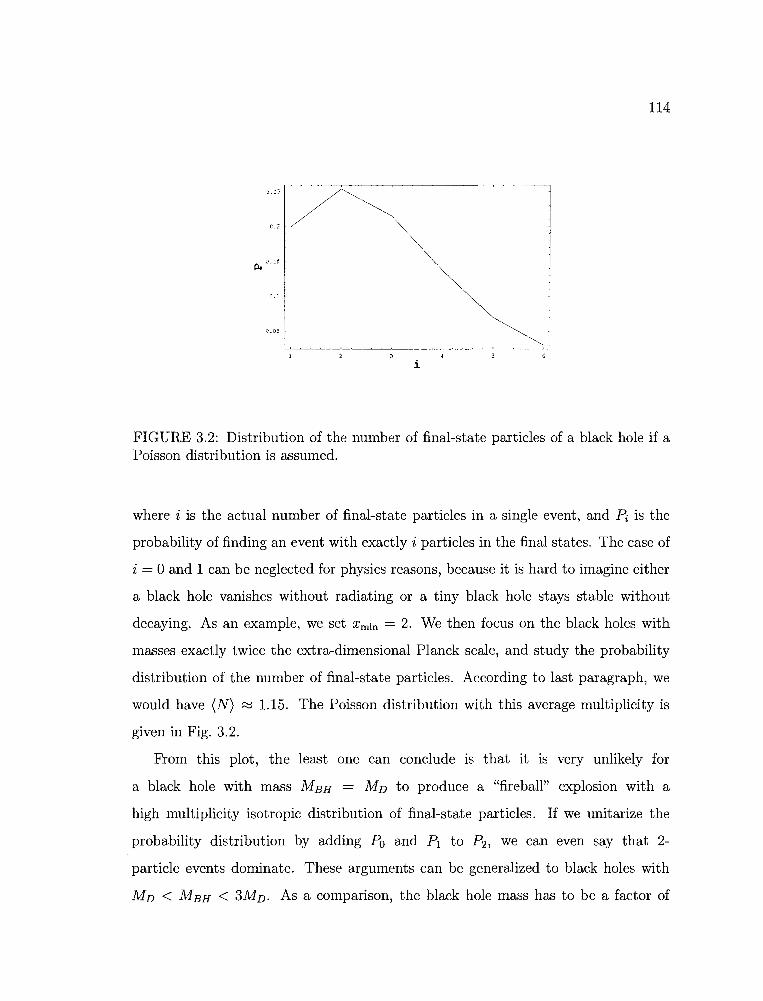
114
i
FIGURE 3.2: Distribution of the number of final-state particles of a black hole if aPoisson distribution is assumed.
where i is the actual number of final-state particles in a single event, and ~ is the
probability of finding an event with exactly i particles in the final states. The case of
i = 0 and 1 can be neglected for physics reasons, because it is hard to imagine either
a black hole vanishes without radiating or a tiny black hole stays stable without
decaying. As an example, we set Xmin = 2. We then focus on the black holes with
masses exactly twice the extra-dimensional Planck scale, and study the probability
distribution of the number of final-state particles. According to last paragraph, we
would have (N) ::;:j 1.15. The Poisson distribution with this average multiplicity is
given in Fig. 3.2.
From this plot, the least one can conclude is that it is very unlikely for
a black hole with mass MBH = MD to produce a "fireball" explosion with a
high multiplicity isotropic distribution of final-state particles. If we unitarize the
probability distribution by adding Po and PI to Pz, we can even say that 2
particle events dominate. These arguments can be generalized to black holes with
MD < MBH < 3MD. As a comparison, the black hole mass has to be a factor of
115
3 times larger than the extra-dimensional Planck scale in order to yield an average
multiplicity around 4. We can get to a very similar conclusion by analyzing the
phase space of final states with different numbers of particles, and the domination of
2-particle events is still favored because the phase space of more final-state particles
is strongly suppressed.
Most of the previous studies used high multiplicity as the signature of finding
a thermal black hole at the LHC. However, we think this approach is impractical
since the proton pairs at the LHC will mostly form black holes at lower energies and
with low multiplicity, if there were any. Those black holes will not qualify as truly
thermal black holes as their masses are below the semi-classical threshold. They are
probably not even real black holes. It would be more precise if we call them "bound
states". Nevertheless these states should exhibit significant gravitational effects. It
seems plausible to us that some of the properties of such states can be extrapolated
from a thermal black hole. We will call such "bound states" quantum black holes
(QBHs) from now.
In order to verify the production of QBHs at the LHC, we need to make a few
assumptions about how it would decay. Thorough study shows that a black hole of
astrophysical size usually goes through several stages before it loses all its energy and
vanishes eventually. Typically, a black hole formed in a particle collision would have
nonzero angular momentum determined by the impact parameter. At particle level,
it is also very likely for the black hole to carry gauge numbers of the initial parton
pairs, which might include both electromagnetic charges and color charges. Moreover,
since the formation occurs in a violent process, the initial event horizon could be
very asymmetric, and hence the black hole could possess extra hair corresponding to
the multi-pole moments of the distribution of gauge charges and energy momentum
within the configuration [30]. Therefore, a black hole formed in this way is believed
by many to go through a four-stage process, including balding, spindown, Hawking
radiation and final explosion.

116
After balding and spindown the black hole can become symmetric by getting rid
of various multi-pole moments and its angular momentum, through classical gauge
radiation to gauge fields on the brane where the standard model fields resides, and
through gravitational radiation. The frequency of the radiation, w, also from a classic
point of view, is obviously determined by the frequency of the oscillation of the multi
pole moments. Naturally, since the typical length scale of those multi-pole moments
is set by the Schwarzschild radius of the horizon, rs , the duration of the balding
process should be rv r;l. On the other hand, the lifetime of an ordinary black hole is
rv MBH . However, for a Planckian QBH, the above two scales are very close, and it
suggests we should not treat balding as a separate stage from the rest of the decay.
We also consider the spin-down process as inseparable from the other stages because
it happens almost instantaneously near the threshold. It is calculated in [31] that for
n = 0, 1 there are upper limits to the angular momentum of the black hole produced
in a grazing collision,
J ~ J* (MBH
) = { (1/2) rsMBH n = 0 (3.28)(2/3) rsMBH n = 1
For MD < MBH < 3MD , the angular momentum is at most of order 1. We assume
these results can be generalized to n 2: 2, and hence we decide not to treat the
spin-down process separately, either.
During the following Hawking radiation and the final explosion as the black hole
mass has diminished down to the Planck scale, it is possible black hole will radiate
to both the brane fields and the modes in extra dimensions, which people call "bulk"
modes. Energy dissipated into the extra dimensions will of course be identified as
missing energy. We show this process in Fig. 3.3. It would have severely undermined
the prospect of observing the decay products of black holes if the black holes were to
lose too much energy to the bulk. In fact, [32] argues the black hole radiates mainly
on the brane. We will simply give a qualitive analysis here [33].

117
",,..- -- ..../ '
,>-----------..~\~~t Black hole )\ .. __._-_._._.-/~
3-mffire '-----/
FIGURE 3.3: An extra-dimensional black hole bound on a 3D brane emits Hawkingradiation to both brane fields and bulk modes. This figure is provided by [30].
As indicated in Eq. (3.24), the Hawking temperature is proportional to the inverse
Schwarzschild radius of the underlying black hole,
(3.29)
(3.30)
This temperature determines a variety of properties of the black hole decay, including
the typical wavelength,
21rA = -T »rs ·
BH
The fact that the wavelength greatly exceeds the size of the horizon implies we should
treat the decaying black hole as a point radiator, and therefore the emission is mostly
in s waves. In other words, the radiation is only sensitive to the radial coordinate,
and the extra angular modes available in the extra dimensions are not important. As
a result, the black hole will decay equally to a particle on the brane and in the bulk.

118
Since there are many more modes on the brane than those in the bulk, the Hawking
radiation is believed to be dominated by Standard Model fields, and we will neglect
the bulk modes from our following discussions.
Summarizing the last few paragraphs, it is unlikely for a black hole near the Planck
scale to shed its multi-pole moments, gauge charge, angular momentum through well
separated processes. The radiation into the extra dimensions from such a black hole
also seems to be irrelevant. As a result, we think it is plausible to think of the decay
of a QBH to be instantaneous, and its quantum numbers will simply be preserved by
a two-body final states which will dominate the phase space of the decay products.
The two particles in the final states are confined on the brane and included in the
Standard Model, and the Compton wavelength of each particle will be of order the
size of the QBH.
3.4 Quantum Black Holes and Cross Sections
3.4.1 What Is a Quantum Black Hole
To state our assumptions more clearly, we first characterize our QBHs by three
quantities: mass, spin and gauge charges. Most importantly, QBHs can have a SU(3)
charge, or equivalently, a color charge, in contrast to the traditional treatment of
black holes where only electromagnetic charges are considered. This characterization
does not contradict the confinement since apparently the hadronization only happens
at a much longer scale (AQCD ) than the QBH formation and decay. The central
assumptions of our study are listed as below in a more formal way:
(I) Processes involving QBHs conserve QCD and U(l) charges sincelocal gauge symmetries are not violated by gravity.
(II) QBH coupling to both on-shell long wavelength and highly off-shellperturbative modes of the Standard Model is suppressed.
(III) QBHs decay democratically to all Standard Model fields as long asassumption I and II are both satisfied.
119
We choose to hold assumption (I) because it is hard to imagine local gauge
charges would be modified by the formation and decay of QBHs. We think the
most reasonable scenario is that the total flux through a large Gaussian 3-sphere
surrounding the spatial region where QBH formation and decay occurs should remain
constant by causality. This implies the conservation of both QCD charges and U(l)
charges. It would be extremely odd if gravity only chooses to violate only one local
gauge symmetry while leaving the other intact. This is the key assumption of our
project, because it leads to the statement that the two-body final states of the QBH
decay would preserve not only the electromagnetic charge of the black hole, or that of
the initial parton pair, but it would also preserve the QCD charge of the initial parton
pair, which enables us to calculate the branching ratios of individual channels of the
decay. In the discussions below, we shall classify QBHs according to the irreducible
representations of SU (3)c and U (l)em' and label QBH states as QBH~. Assumption
(II) is necessary so that the precision measurements, or possibly proton decay would
not force the quantum gravity scale to be much larger than the TeV scale.
It is worth mentioning that our results for the decay of QBHs also depend on
whether we require QBH processes correspond to Lorentz invariant local effective
field theory operators. We are not aware of any argument in favor of this which
is as robust as that for the conservation of QCD charge. However, even if Lorentz
invariance is indeed violated by quantum gravity in QBH processes, we can still
employ assumption (II) to avoid any contamination from those effects in low energy
physics near 1 TeV. We will come back to this with more details later.
3.4.2 Inclusive Cross Sections
In order to get quantitative results for we shall assume that QBH production
cross sections can be extrapolated from the cross sections obtained for semi-classical
black holes. We rewrite Eq. (3.18) by putting in the parameter Xmin == MminBH/MD,
t 2zdz t 2 du t dv F (n) .io J:mi?zMD Ju v
y s
. 1rr; (US, n, M D ) L fa (u/v, Q) fb (v, Q)a,b
120
(3.31)
Originally, the input for Xmin, as we illustrated earlier, is around 3 or 4 so that one
can derive numerical results for cross sections of the production of semi-classical
black holes. In our case, Xmin is chosen to be only 1 in order to calculation the
production rates of QBHs which have limited entropy and mostly decay to only
two particles in the final states. The construction for black hole production from
high-energy collisions by Eardley and Giddings in [34] is held to be true for a QBH
process as well in our calculation. To complete numerical analysis we use CTEQ5
PDFs and leave it to the users of our numerical program to decide whether to let
the momentum transfer Q to be rv M D or r;l. We have also fitted the functions Yz
for different numbers of compactified dimensions to the curves given by Nambu and
Yoshino in [25J. For comparison we will calculate cross sections of semi-classical black
hole production as well by setting Xmin = 3, and confirm our previous assumption that
most of the c.m. energy will be lost through Initial-state Radiation and gravitational
waves so that QBHs will dominate beyond the extra-dimensional Planck scale at the
LHC.
3.4.3 Conservation of Gauge Charges
Finally we are ready to discuss the conservation of gauge charges in QBH
processes. As mentioned earlier, QBHs can form representations of the SU (3)c group
and carry a QED charge at the same time. We denote the process of two partons
Pi ,Pj forming a QBH in the c representation of the SU(3) group of electric charge q
Pi + Pj -----* QBH~ . (3.32)
121
In quantum chromodynamics, quarks resides in 3, the fundamental representation of
SU(3), which is simply named by the dimension of this irreducible representation.
This same rule of notation will apply to any other irreducible representation as
well. Anti-quarks are described by the conjugate representation of the fundamental
representation, 3, while gauge transformation property of gluons resemble the
irreducible representation known as the adjoint representation, 8. The color
representation of QBHs should be equivalent to the direct product of the color
representations of the initial parton pair. For example, a quark and an anti-quark
form a representation of 3 ® 3, the direct product of 3 and 3. In group theory, this
representation that results from a direct product can be decomposed to two separate
irreducible representations:
(3.33)
where 1 denotes a color singlet that transforms to itself under the SU(3) group.
In colliders, Eq. (3.33) corresponds to the transition of a quark and an anti-quark
forming either a singlet QBH or an octet QBH which transforms under SU(3) in the
adjoint representation. There is no a priori knowledge that can help us determine
the exact likelihood of producing QBHs in different irreducible representations, but
it seems to us the most natural assumption we can make about this is:
(IV) The probability to create a QBH within an irreducible representationduring a given transition process is proportional to the dimension ofthe irreducible representation.
Consequently, the probability to find a color-singlet QBH produced by a quark-anti
quark pair is 1/9, while the probability to find a color-octet QBH in the same reaction
is 8/9. For completeness, we list all the other direct products of representations and
their decompositions that are relevant to parton pairs forming QBHs~ as below:
122
3®3 6EB3 (3.34)
3®8 3 EB 6 EB 15 (3.35)
8®8 Is EB 8s EB 8A EB 10 EB 1-0A E.B 27s , (3.36)
where the lower index "A" means "anti-symmetric" and "8" means "symmetric".
An tensor object within a representation can be either symmetric or anti-symmetric
under the exchange of two of the tensor indices. On the other hand, the decay
product of a QBH should inherit the color charge of the same QBH according to
our assumption (I). We shall use a specific example to illustrate this color charge
conservation. Consider a quantum black hole with electric charge -2/3 and color
charge 3. A QBH will decay to a final state consisting of two standard model particles
as pointed out earlier, which by themselves could be color-singlets (leptons, 8U(2)
gauge bosons, Higgs), color-triplets (quarks and anti-quarks) or color-octets (gluons).
The direct products of the color representations of those two particles must have a
non-zero overlap with the color representation of the mother black hole, otherwise
the transition channel would be forbidden by assumption (I). As a result, possible
final states could be made up of two down-type quarks, one anti-up-quark plus a
neutrino, and all other particle combinations that could yield a color charge of "3"
and an electric charge of -2/3. Each individual degrees of freedom will have the same
branching ratio since we consider a QBH to be an extrapolation of a semi-classical
black hole and thus decay democratically to standard model fields. Other constraints
could apply if a local field theory description is relevant and if Lorentz invariance is
held to be true at the QBH scale. More decay channels and corresponding branching
ratios will be covered later.
There are some other issues that remain to be clarified. In a local field theory
description that respects Lorentz invariance, we assume a transition is probable as
long as a local field operator for that same reaction can be written down. This

123
treatment is also justified by the observation that the decay of a Planckian black
hole should be dominated by S waves, since black holes near the threshold are much
smaller in size compared to the typical wavelength of the radiation and thus act like
point radiators. Furthermore, we adopt this treatment because we believe the angular
momentum of a QBH that comes from a nonzero impact parameter is extremely
small and can be neglected from numerical considerations, which is supported by the
calculation of [31]. The angular momentum conservation can therefore be taken care
of by constraining the local field operator to preserve Lorentz invariance. However,
more channels will be open if we relax the requirement on Lorentz invariance, and
one would have more striking signatures of QBHs in that way.
Another problem is related to the numerical integrations present in Eq. (3.31).
The integrand changes drastically within the domain of integration due to the effects
of PDFs. As a result, ordinary Monte Carlo integration might not be appropriate
for our purpose which would converge very slowly in this case. Instead, a integration
package developed by M. Martinez, J. Illana, J. Bossert, and A. Vicini is used to
evaluation the integral in Eq. (3.31) and many other integrals that will introduced
later. The algorithm this package makes use of is known as VEGAS. It acquires better
convergence over ordinary Monte Carlo integration through importance sampling and
stratified sampling. VEGAS starts the integration at interest with a uniform stratified
distribution, and evolve the stratified distribution adaptively by histogramming the
integrand in order to achieve a better resemblance of the shape of the integrand.
A separable probability function is used as the stratified distribution function when
dealing with multi-dimensional integrals,
(3.37)
such that the number of histogram bins will only increase as K d instead of K d if
there are K bins for each coordinate and d dimensions in total.

124
3.4.4 Individual Decay Channels
We have assumed that QBH processes will conserve both color charge and electric
charge, and this is one of the governing rules that determine the decay process of
QBHs. An example is already given as we mention the possible decay products of
QBH;2/3. QBHs with other gauge charges will be discussed below under different
assumptions about Lorentz invariance.
Let us begin with a color-singlet QBH that is also neutral under U (l)em' or,
QBH~ . In our setup, such a black hole can decay to any combinations of Higgs
bosons, leptons, quarks as well as gauge bosons and gravitons, e.g.
QBH? -----t e+ + e- ,
QBH? -----t e++j1- ,
QBH? -----t qi + iii , (3.38)
etc., as long as we do not impose Lorentz invariance and the global final state is
neutral under SU(3) and U (1)em' The number of degrees of freedom of a quark
anti-quark pair a QBH? can decay to is three times that of a lepton pair, since there
are three different colors. Similarly, the number of degrees of freedom of a pair of
ZO bosons is ~ x ~ = 9/4 times that of a lepton pair, since there are 3 degrees of
freedom in spin space for a massive gauge boson while only 2 for a fermion. We
follow these rules when developing the branching ratios for individual channels based
on the particle level cross sections of a certain type of QBH, which in this case is just
QBH? The integral that need to be evaluated is simply Eq. (3.31) with the sum over
parton pairs modified in order to account for the right combination of gauge charges.
For a color-singlet black hole with zero electric charge, we select to sum over only
neutral quark-anti-quark pairs, and then multiply the resulting integral by a factor
of 1/9, according to the color representation argument we give above. Apparently,
125
most of the time QBH~ would decay into two-jet events due to the large number of
color degrees of freedom.
A color-octet black hole which is electromagnetically neutral, QBHg, can decay
into a pair of a quark and an anti-quark with opposite electric charge, or a gluon
and a neutral particle, e.g., a graviton or a Z-boson. More details on the branching
ratios depend on how many independent channels there are. The availability of any
specific channel can be affected by whether one wants to enforce a Lorentz invariant
local field theory description of the QBH reaction. If we do assume this particular
description of QBH processes, then transitions such as
(3.39)
would not be allowed, where qi are quarks and 9 is gluon, because there is no way
to write down a Lorentz invariant local field operator linking three fermions and a
spin-1 gauge boson.
An electrically charged color-triplet black hole, QBH~, can decay to either a pair
of a charge q quark and a gluon, or a pair of anti-quarks, depending on the initial
configuration of the parton pair that forms the same QBH. However, those two types
of events are both characterized by two back-to-back jets in the final state, and
thus are difficult to be separated from the Standard Model background. Other
similar modes may include quark + photon, quark + Z-boson, anti-quark + anti
neutrino, etc. The decay products of black holes in higher representations can also
be determined in this way: QBH?a, QBH?-a, QBHg7 , QBH~, QBHi5' QBH~ and QBH§.
In this project, we study the QBH cross sections in three different scenarios that
can give rise to the production of QBHs near the 1 TeV scale. We will not review
ADD and RS here since both of them have been well known and explored. We
will only briefly discuss a new four-dimensional model here that is suggested by
Xavier Calmet, Stephen Hsu and David Reeb [35]. In an ordinary extra-dimensional
model, the Planck scale is lowered to the TeV scale because the large volume of extra
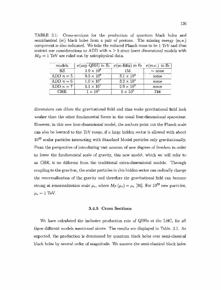
126
TABLE 3.1: Cross-sections for the production of quantum black holes andsemiclassical (sc) black holes from a pair of protons. The missing energy (m.e.)component is also indicated. We take the reduced Planck mass to be 1 TeV and thusrestrict our considerations to ADD with n ~ 5 since lower dimensional models withM D = 1 TeV are ruled out by astrophysical data.
models o-(any QBH) in fb o-(sc-BHs) in fb o-(m.e.) in fbRS 1.9 X lOti 151 '" none
ADD n = 5 9.5 x 10° 3.1 X 10⁴ someADD n = 6 1.0 X 10 1 3.2 X 10'1 someADD n = 7 1.1 X 101 2.9 X 10'1 some
CHR 1 x W) 5 X lOiS 744
dimensions can dilate the gravitational field and thus make gravitational field look
weaker than the other fundamental forces in the usual four-dimensional spacetime.
However, in this new four-dimensional model, the authors point out the Planck scale
can also be lowered to the TeV range, if a large hidden sector is allowed with about
1032 scalar particles interacting with Standard Model particles only gravitationally.
From the perspective of introducing vast amount of new degrees of freedom in order
to lower the fundamental scale of gravity, this new model, which we will refer to
as CHR, is no different from the traditional extra-dimensional models. Through
coupling to the graviton, the scalar particles in this hidden sector can radically change
the renormalization of the gravity and therefore the gravitational field can become
strong at renormalization scale J.L*, where M p (J.L*) = J.L* [36]. For 1032 new particles,
J.L* rv 1 TeV.
3.4.5 Cross Sections
We have calculated the inclusive production rate of QBHs at the LHC, for all
three different models mentioned above. The wmlts are displayed in Table. 3.1. As
expected, the production is dominated by quantum black holes over semi-classical
black holes by several order of magnitude. We assume the semi-classical black holes
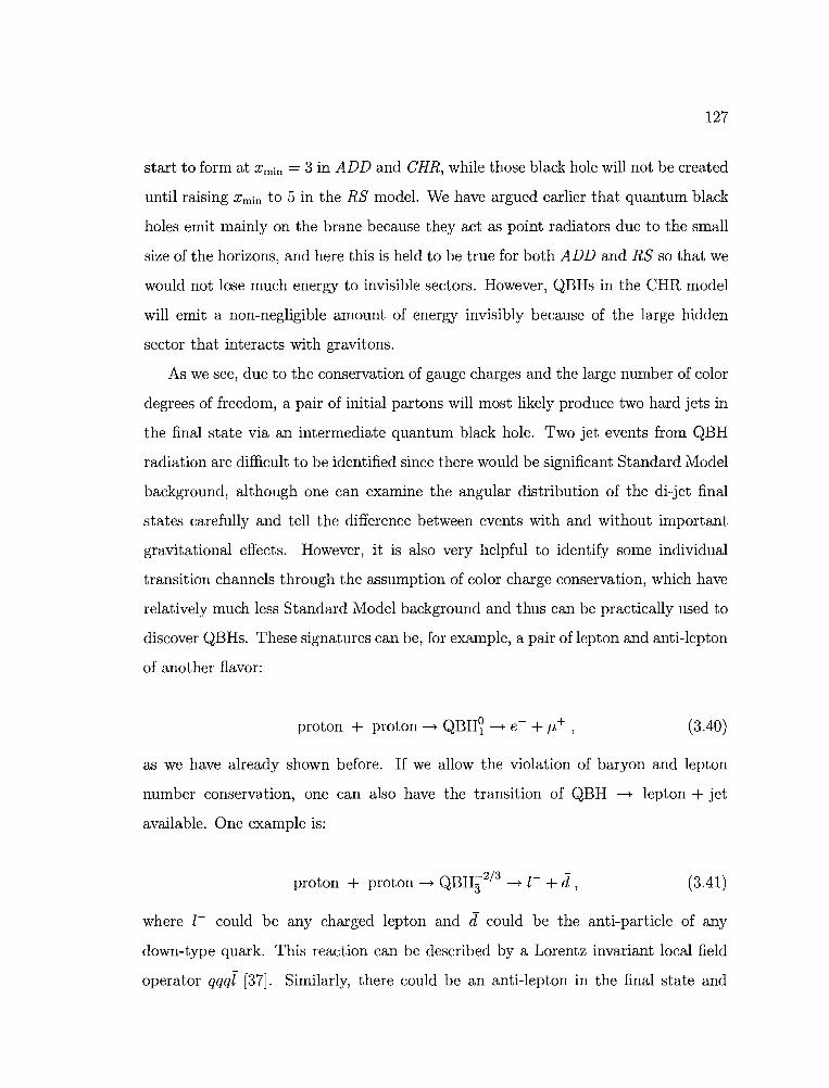
127
start to form at Xmin = 3 in ADD and CHR, while those black hole will not be created
until raising Xmin to 5 in the RS model. We have argued earlier that quantum black
holes emit mainly on the brane because they act as point radiators due to the small
size of the horizons, and here this is held to be true for both ADD and RS so that we
would not lose much energy to invisible sectors. However, QBHs in the eHR model
will emit a non-negligible amount of energy invisibly because of the large hidden
sector that interacts with gravitons.
As we see, due to the conservation of gauge charges and the large number of color
degrees of freedom, a pair of initial partons will most likely produce two hard jets in
the final state via an intermediate quantum black hole. Two jet events from QBH
radiation are difficult to be identified since there would be significant Standard Model
background, although one can examine the angular distribution of the di-jet final
states carefully and tell the difference between events with and without important
gravitational effects. However, it is also very helpful to identify some individual
transition channels through the assumption of color charge conservation, which have
relatively much less Standard Model background and thus can be practically used to
discover QBHs. These signatures can be, for example, a pair of lepton and anti-lepton
of another flavor:
proton + proton -----+ QBH~ -----+ e- + J1,+ , (3.40)
as we have already shown before. If we allow the violation of baryon and lepton
number conservation, one can also have the transition of QBH -----+ lepton + jet
available. One example is:
proton + proton -----+ QBHj-2/3 -----+ Z- + d , (3.41)
where Z- could be any charged lepton and d could be the anti-particle of any
down-type quark. This reaction can be described by a Lorentz invariant local field
operator qqqZ [37]. Similarly, there could be an anti-lepton in the final state and
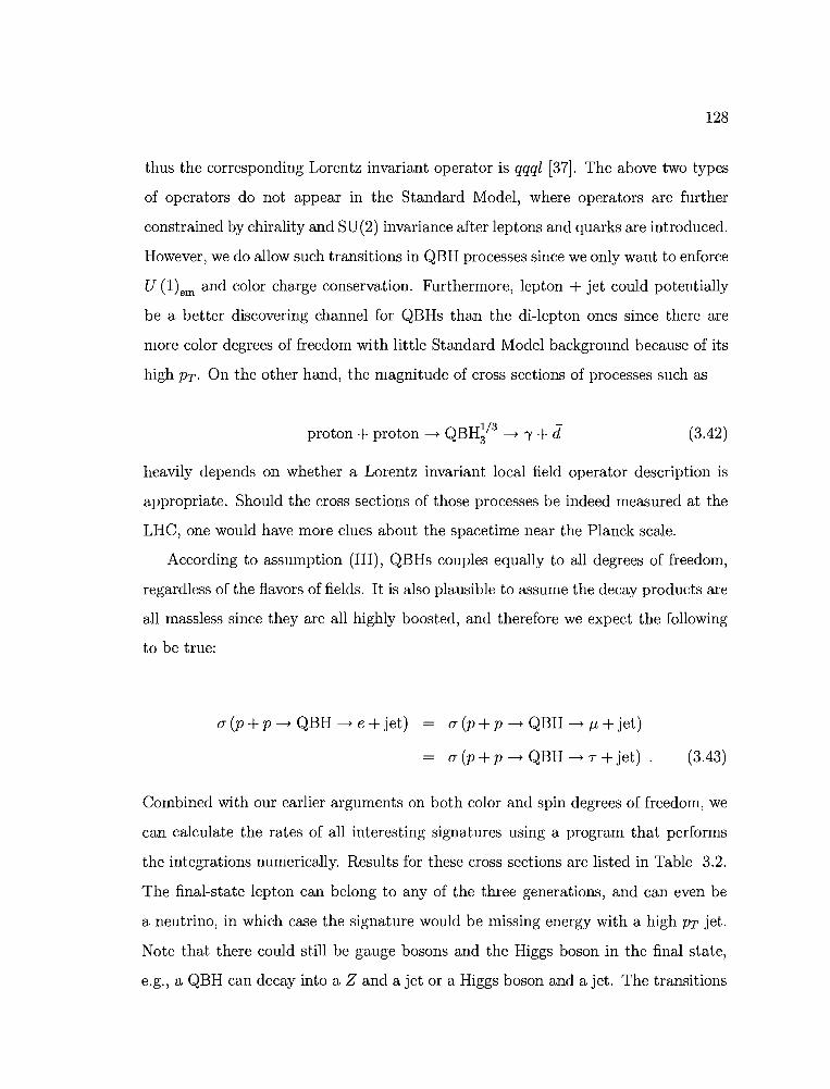
128
thus the corresponding Lorentz invariant operator is qqql [37]. The above two types
of operators do not appear in the Standard Model, where operators are further
constrained by chirality and SU(2) invariance after leptons and quarks are introduced.
However, we do allow such transitions in QBH processes since we only want to enforce
U (l)em and color charge conservation. Furthermore, lepton + jet could potentially
be a better discovering channel for QBHs than the di-Iepton ones since there are
more color degrees of freedom with little Standard Model background because of its
high PT. On the other hand, the magnitude of cross sections of processes such as
1/3 -proton + proton -t QBH3 -t, + d (3.42)
heavily depends on whether a Lorentz invariant local field operator description is
appropriate. Should the cross sections of those processes be indeed measured at the
LHC, one would have more clues about the spacetime near the Planck scale.
According to assumption (III), QBHs couples equally to all degrees of freedom,
regardless of the flavors of fields. It is also plausible to assume the decay products are
all massless since they are all highly boosted, and therefore we expect the following
to be true:
(J (p + P -t QBH -t e + jet) (J (p + P -t QBH -t J.,l + jet)
(J (p + P -t QBH -t T + jet) (3.43)
Combined with our earlier arguments on both color and spin degrees of freedom, we
can calculate the rates of all interesting signatures using a program that performs
the integrations numerically. Results for these cross sections are listed in Table 3.2.
The final-state lepton can belong to any of the three generations, and can even be
a neutrino, in which case the signature would be missing energy with a high PT jet.
Note that there could still be gauge bosons and the Higgs boson in the final state,
e.g., a QBH can decay into a Z and a jet or a Higgs boson and a jet. The transitions
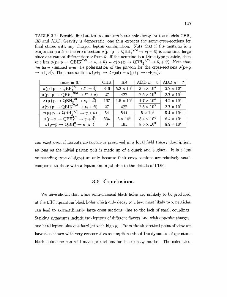
129
TABLE 3.2: Possible final states in quantum black hole decay for the models CHR,RS and ADD. Gravity is democratic; one thus expects the same cross-sections forfinal states with any charged lepton combination. Note that if the neutrino is aMajorana particle the cross-section a(p+p -+ QBHi2/3 -+ Vi + it) is nine time largesince one cannot differentiate V from D. If the neutrino is a Dirac type particle, thenone has a(p+p -+ QBHi2/3 -+ Vi + it) = a(p+p -+ QBHi2/3 -+ Di + it). Note thatwe have summed over the polarization of the photon for the cross-sections a(p+p-+ i+jet). The cross-section a(p+p -+ Z+jet) = a(p+p -+ i+jet).
rates in fb CHR RS ADD n = 6 ADD n = 7a(p+p -+ QBH~/3 -+ Z+ + d) 346 5.3 x 10³ 3.5 X 10⁴ 3.7 X 10⁴
a(p+p -+ QBH;2/3 -+ Z- + d) 27 422 2.5 x 10³ 2.7 X 10³
a(p+p -+ QBH~/3 -+ Vi + d) 167 1.5 x 10³ 1.7 X 10⁴ 4.2 X 10⁴
a(p+p -+ QBH;2/3 -+ Vi + it) 27 422 2.5 x 10³ 2.7 X 10³
a(p+p -+ QBH;2/3 -+ i + it) 54 844 5 x 10³ 5.4 X 10³
a(p+p -+ QBH~/3 -+ i + d) 334 3 x 10³ 3.4 X 10⁴ 8.4 X 10⁴
a(p+p -+ QBH~ -+ e-t- /-L ) 0 161 8.5 x 1O:t 8.9 X 10:t
can exist even if Lorentz invarience is preserved in a local field theory description,
as long as the initial parton pair is made up of a quark and a gluon. It is a less
outstanding type of signature only because their cross sections are relatively small
compared to those with a lepton and a jet, due to the details of PDFs.
3.5 Conclusions
We have shown that while semi-classical black holes are unlikely to be produced
at the LHC, quantum black holes which only decay to a few, most likely two, particles
can lead to extraordinarily large cross sections, due to the lack of small couplings.
Striking signatures include two leptons of different flavors and with opposite charges,
one hard lepton plus one hard jet with high PT. From the theoretical point of view we
have also shown with very conservative assumptions about the dynamics of quantum
black holes one can still make predictions for their decay modes. The calculated

130
branching ratios for such channels are sufficiently big and numerous interesting events
can be generated at the LHC, given our four central assumptions.

131
CHAPTER IV
DIRECT NUMERICAL INTEGRATION
4.1 Introduction
At the LHC era, the Standard Model cross sections of many transitions, where
2 particles scatter to produce n other particles, are important for the discovery of
new physics beyond the Standard Model itself. At the lowest order in perturbation
theory, the calculation of such cross sections is straightforward. One can simply
multiply the squared tree-level matrix elements by the measurement function for
each choice of final-state momentum {Pl,PZ, ... ,Pn}, and then integrate over these
momentum either numerically or analytically without too much trouble, since there
are no singularities present.
However, it is not trivial to extend the same calculation to the next-to--Ieading
order. A matrix element with one virtual loop needs to be multiplied with both the
complex conjugate of the tree-level matrix element and the measurement function,
plus the complex conjugate of this product. To calculate the corresponding cross
section, one can typically choose to compute the loop integral first within the loop
diagram, and use the result as a whole to be the integrand of the integration over
the final state momentum. It is unavoidable that people would run into infrared
and ultraviolet divergences during the loop integration, and that is exactly what
makes such NLO evaluations difficult. Necessary subtraction schemes would have
to be adopted to control the divergences. People have been devising algorithms to
decompose those loop integrals with multiple external legs using a series of the so-

...._._-------------
132
called "master integrals", for which values are known. There has been rapid progress
in this approach recently [38:1[39][40J.
Another methodology is to perform the loop integral numerically. The idea is
to integrate the loop momenta l of the loop diagram with the group of external
momentum {Pl,P2, ... ,Pn} altogether at the same time when evaluating the product
of the amplitude of the virtual loop diagram and that of the complex conjugate of
the tree-level diagram. This means one sample point for the numerical integration
in a Monte Carlo style algorithm would be simply {l;Pl,P2, ... ,Pn}. However, the
loop amplitude still contains factors such as 1/ ((l- Qi)2 + if), which gives rise to
singularities. The numerical approach can set up schemes where some of the above
singularities can be avoided through deforming the integration contour away from
the singular point into the complex l space. The essential problem is how to specify
the contour deformation in a systematic way when there are multiple singular factors
present in the integrand. One choice is to use the Feynman parameters, x, to rewrite
the integrand so that the loop integral can be integrated over l and x or even only
x. Then the mission becomes deforming the contour of x in the complex plane. It is
still categorized as the numerical Monte Carlo method because every set of Feynman
parameters x (there could be more than one Feynman parameter in a single loop
integral) will be sampled with a choice of the external momentum.
In [41J, an example is given for using Feynman parameters to integrate the loop
momenta numerically. The process studied is the scattering of
(4.1)
through a massless electron loop. The virtual loop diagram with 6 external photons
is shown in Fig.4.1. According to Feynman rules, the matrix element that correponds
to this diagram is
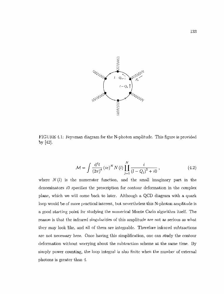
133
FIGURE 4.1: Feynman diagram for the N-photon amplitude. This figure is providedby [42].
/
d4l N.M - -- ie N N l Z
- (27ft () ( )D(l - Qj)2 + iO '(4.2)
where N (l) is the numerator function, and the small imaginary part in the
denominators iO specifies the prescription for contour deformation in the complex
plane, which we will corne back to later. Although a QCD diagram with a quark
loop would be of more practical interest, but nevertheless this N-photon amplitude is
a good starting point for studying the numerical Monte Carlo algorithm itself. The
reason is that the infrared singularities of this amplitude are not as serious as what
they may look like, and all of them are integrable. Therefore infrared subtractions
are not necessary here. Once having this simplification, one can study the contour
deformation without worrying about the subtraction scheme at the same time. By
simply power counting, the loop integral is also finite when the number of external
photons is greater than 4.
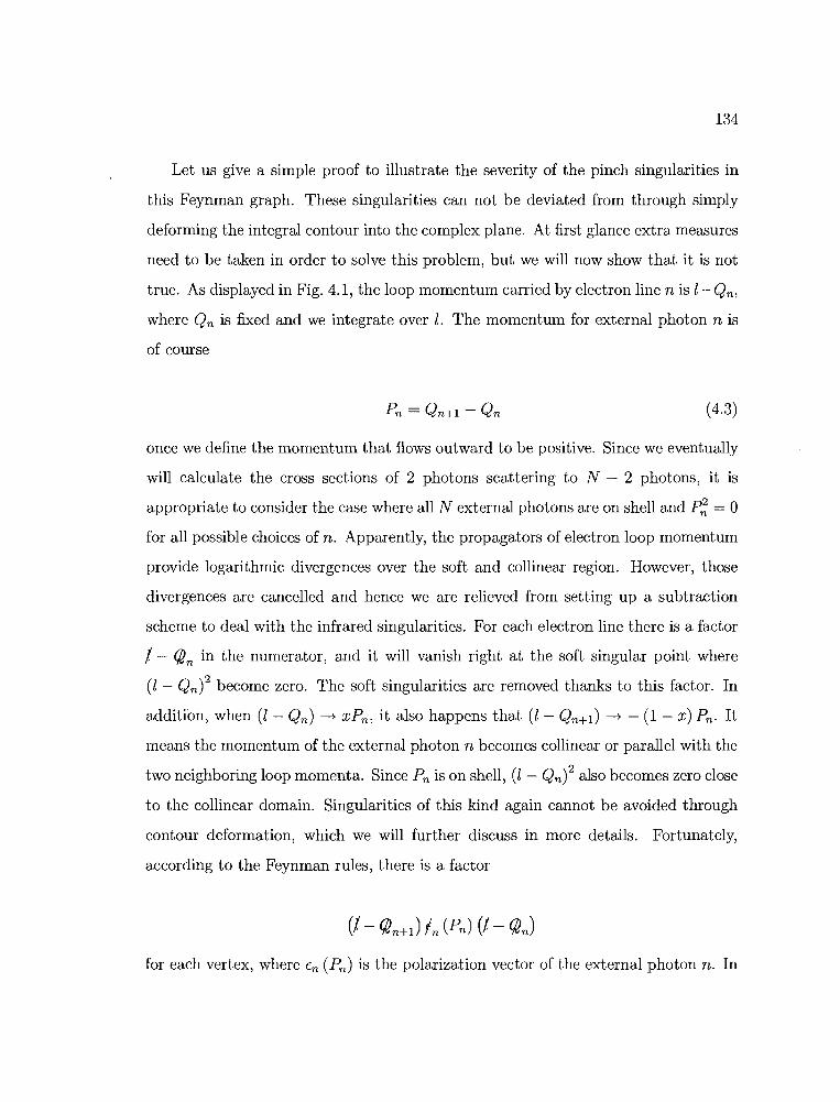
134
Let us give a simple proof to illustrate the severity of the pinch singularities in
this Feynman graph. These singularities can not be deviated from through simply
deforming the integral contour into the complex plane. At first glance extra measures
need to be taken in order to solve this problem, but we will now show that it is not
true. As displayed in Fig. 4.1, the loop momentum carried by electron line n is l-Qn,
where Qn is fixed and we integrate over l. The momentum for external photon n is
of course
(4.3)
once we define the momentum that flows outward to be positive. Since we eventually
will calculate the cross sections of 2 photons scattering to N - 2 photons, it is
appropriate to consider the case where all N external photons are on shell and P~ = 0
for all possible choices of n. Apparently, the propagators of electron loop momentum
provide logarithmic divergences over the soft and collinear region. However, those
divergences are cancelled and hence we are relieved from setting up a subtraction
scheme to deal with the infrared singularities. For each electron line there is a factor
t - Qn in the numerator, and it will vanish right at the soft singular point where
(l - Qn)2 become zero. The soft singularities are removed thanks to this factor. In
addition, when (l - Qn) ---+ xPn, it also happens that (l - Qn+l) ---+ - (1 - x) Pn. It
means the momentum of the external photon n becomes collinear or parallel with the
two neighboring loop momenta. Since Pn is on shell, (l- Qn)2 also becomes zero close
to the collinear domain. Singularities of this kind again cannot be avoided through
contour deformation, which we will further discuss in more details. Fortunately,
according to the Feynman rules, there is a factor
for each vertex, where En (Pn ) is the polarization vector of the external photon n. In
135
the collinear limit when (l - Qn) -----+ xP, we can use a little bit of the gamma matrix
algebra and derive
We require En (Pn ) . Pn = 0 because photon as a massless gauge boson can only have
transverse degrees of freedom and hence be transversely polarized. This automatically
removes collinear divergences from our consideration.
Back to the Feynman parameter approach, Eq. (4.2) can be rewritten down as
M
(4.5)
where £ is the spatially translated and Wick rotated loop momentum, and therefore
£.£ is in fact the Euclidean square of l. A2 (x) is a quadratic function of the Feynman
parameters, and C is the integration contour over which x's are integrated.
Since all singularities left in Eq. (4.5) are integrable, it is in principle guaranteed
the numerical integration will converge given enough sample points in a Monte Carlo
style calculation. However, a numerical algorithm is only useful when it can reduce
the statistical uncertainty to an acceptable degree with a practical number of sample
points. Thus the contour C of the Feynman parameters are carefully chosen [41],
instead of randomly picked, to stay away from singularities whenever it is possible.
It turns out the maximum number of external photons, for which such a numerical
calculation can give a sensible answer on an ordinary computer, is N = 6. The
numerical integral introduced in Eq. (4.5) would fail to converge fast enough for N >
6. For several helicity configurations (of the external photons), there are analytical
solutions, and the numerical results have been found to agree with the analytical
results.
136
There are limitations to the Feynman parameter method. As the number of
external photons increases, the power of the quadratic function A (x) also goes up, and
this can make the numerical convergence worse, although theoretically the integral
will converge eventually. Moreover, if a calculation is encountered where the infrared
subtraction is needed, people would not be able to construct any subtraction scheme
within the framework of the Feynman parameter approach. In contrast, it is already
known [43] how to construct subtractions directly in the momentum space. It would
be therefore very nice if one can specify a way to perform the numerical integral
directly in the momentum space, without the help of Feynman parameters.
The most difficult issue concerning a direct numerical integration would be the
determination of the contour of the integral. The Feynman parameter is free of this
problem because the singular denominator is the power of a quadratic function, A (x),
of the integration variables. It is very simple to find a contour that can be diverted
away from all the roots of the quadratic equation A (x) = O. However, as Eq. (4.2)
shows, there are many different factors in the denominator in the direct approach, and
the singularities are scattered out in a manner for which it is not trivial at all to find an
appropriated deformed contour in the loop momentum space. It is thus the objective
of this project to specify the contour deformation, and compare the numerical results
with those derived by the Feynman parameter method and the analytical answer.
The expectation is, as implied earlier, compared to the Feynman parameter method
the direct numerical integration should be able to calculate virtual loop diagrams
with more external photons. Even if it were only as good as the Feynman parameter
method, we would still be glad to have an algorithm in which the infrared subtraction
can be applied straightforwardly. The standard methodology where M is evaluated
as whole in terms of master integral might still be found to be superior to our new
numerical algorithm, but nevertheless it is still worthwhile to invent new tools and
methods which could turn out to be useful in some other contexts.
137
4.2 Contour Deformation
4.2.1 Generic Form
In Eq. (4.2), the integrand is singular on the surface of (l - Qjf It is a
lightcone with its vertex at Qj in the loop momentum space. People can avoid those
singularities by deforming the loop momentum into the complex plane. The general
technique is to add a small imaginary part to the original momentum, and thus the
deformed momentum becomes a vector function of the original loop momentum:
Pit (l) = lit + iK/t (l) , (4.6)
where ,."It are all real, and they are the components of a 4-vector. After making this
deformation, there will be a new imaginary term showing up in the denominators of
electron propagators, and people will no longer run into singularities on the surface
of the lightcones as long as the imaginary parts do not vanish. In addition, the value
of the deformed integral will remain the same as what the original value is if the
following criterions are satisfied:
(I) The deformation starts in the direction specified by the "+iO"prescription, meaning the imaginary part should be positive whenclose to the original singularities;
(II) The contour should not encounter any other singularities when it isdeformed away from the original singularities.
A simple proof of the above argument can be found in [44]. If we convert the
integration variables of the deformed integral from Pback to l, we would have
M=J d4l4(-ietdet(8P/8l)N(P(l))IT i 2' (4.7)(21T) j=1 (P - Qj)
for a virtual loop diagram with N photons.

138
Since the contour we study is deformed in a vector space, we need to specify both
the direction and the magnitude of the deformation. It would thus be helpful to
rewrite the imaginary part as
(4.8)
and in this expression, A(l) is the real function of momentum that controls the size of
the deformation at each point on the contour. The lower limit of this function is zero
everywhere, and the upper limit At shall be constrained by the second criteria for
contour deformation mentioned earlier, that is, the deformation should be stopped
before the contour hits any other new singularities. If using Eq. (4.8) to express the
denominator for propagator j in Eq.(4.7), one would have
By construction, A(l) ----+ 0 when one just starts the deformation, and the contour
is very close to the original singularities. Geometrically speaking, it also means the
integration variable l would be on the surface of one or more lightcones. Therefore, in
order to retain the value of the original integral, one must have A(l) (l - Qj )'''''0 (l) > 0
on the lightcones so that the +iO prescription can be satisfied. Again, the geometric
interpretation of this requirement is the 4-vector ""0 must be pointing toward the
interior of the lightcone. This can be easily proved by considering an arbitrary l on
the cone where the condition (l - Qj)2 is automatically met. If the corresponding
point l + A""O is indeed in the interior of the cone j, it would be a light-like point and
have
(4.10)
One can make use of the fact (l - Qj)2 = 0 and expand the left hand side of Eq. (4.10)
to the first order in A assuming A is a small parameter. It would come out that

139
). (l - Qi) . /1;0 > O. This proof also works the other way around. More over, it can be
shown in the same way that (l - Qj) . /1;0 = 0 means the vector /1;0 is tangent to the
cone surface.
Ideally, one would want to move the contour away from singularities whenever it
is possible. When there is only one cone j involved, that means, according to the
discussion above, we should let /1;0· (l - Qj) > O. However, it is only true when l is not
on the vertex of that cone, otherwise it is impossible to deform if l- Q j = O. We call it
a "pinch singularity" when the singularity cannot be avoided by making deformations.
In this case, the soft singularity is pinched, but fortunately the analytical divergences
can be removed by a corresponding numerator function as we already pointed out
earlier. The numerical values of the integrand near soft singularities could still be
large and undermine the numerical convergence of the whole integral. A special
technique will be introduced later to resolve this issue by sampling more points near
pinch singularities in a Monte Carlo style calculation.
Things are a little more complicated when momentum l is on more than one
lightcones at the same time. With the help of the geometric interpretation of /1;0 that
satisfies the +iO prescription, however, we can still see what /1;0 should look like in
the momentum space without a problem. One typical situation is when two cones
intersect, how should we manage the contour right on the intersection? Suppose the
vertex of one of the two cones is Qi and the vertex of the other is Qj. If Qj - Qi is
timelike, obviously the singularities on the intersection are not pinched, because we
can easily specify a /1;0 that points to the common interior of both cones, e.g.,
(4.11)
Through simple vector summation, one would find /1;0 defined as such does point
to the correct direction. We can of course prove the same argument by calculating
/1;0· (l- Qi). Since (l - Qi)2 = 0, the /1;0 given in Eq. (4.11) can lead to

140
(4.12)
and straightforwardly this dot product is positive because it is the product of one
timelike vector and one lightlike vector both in the same direction in time. One can
prove this same /);0 also satisfies the same requirement for cone j, and hence confirm
the claim that the contour is deformed in the right direction. If Qj - Qi is instead a
spacelike vector, a /);0 can be easily found in a similar way as well.
If Qj - Qi is lightlike, it means the two loop momentum, l - Qi and l - Qj, are
next to each other in the electron loop, and vector K == Qj - Qi must be equal to
the momentum of the external photon between these two loop momentum up to a
sign. Any l on the intersection of the two corresponding lightcones will make the
. loop momentum collinear with K, and we can parameterize l - Qi = xK. If x < 0
or x > 1, the inside of one cone is inside the other cone, so apparently a /);0 can be
pointing to the interior of both cones when it points to the interior of the inner cone.
However, as pointed earlier, collinear singularities exist when 0 < x < 1, because
the interior of one cone is always outside the other cone. It is thus impossible to
deform the contour into the complex plane in the right direction. To satisfy the
+iO prescription, the only thing one can do is to choose /);0 (x) = c (x) K on the
intersection with 0 < x < 1 so that neither (l - Qi) . /);0 nor (l- Qj) . /);0 is negative.
4.2.2 Geometric Configuration
One can have more specific discussion on the contour deformation with the help of
Fig. 4.2, in which vertices of lightcones and external momenta are suitably visualized.
This plot shows a coordinate system for the loop momentum l, as used in Eq. (4.7),
and this coordinate system is carefully chosen so that the transverse components
of incoming photons vanish. Soft singularities, l = Qi, are shown as black dots in
this sketch, where no contour deformations can be made. Lines joining those end
points are the collinear singularities, l = Qi + X (Qi+l - Qi) where 0 < x < 1.
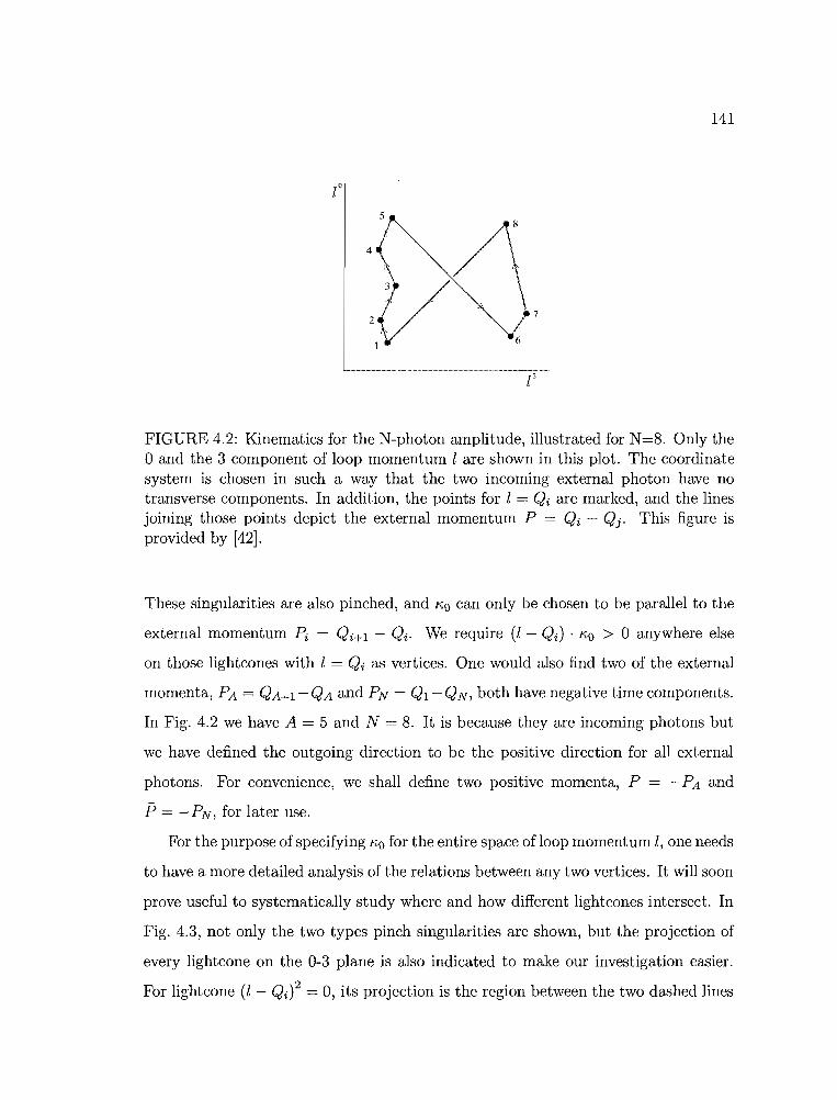
141
FIGURE 4.2: Kinematics for the N-photon amplitude, illustrated for N=8. Only theoand the 3 component of loop momentum l are shown in this plot. The coordinatesystem is chosen in such a way that the two incoming external photon have notransverse components. In addition, the points for l = Qi are marked, and the linesjoining those points depict the external momentum P = Qi - Qj. This figure isprovided by [42].
These singularities are also pinched, and /'\:0 can only be chosen to be parallel to the
external momentum Pi = Qi+l - Qi. We require (l - Qi) . /'\:0 > 0 anywhere else
on those lightcones with l = Qi as vertices. One would also find two of the external
momenta, PA = QA+I-QA and PN = QI-QN, both have negative time components.
In Fig. 4.2 we have A = 5 and N = 8. It is because they are incoming photons but
we have defined the outgoing direction to be the positive direction for all external
photons. For convenience, we shall define two positive momenta, P = - PA and
p = - PN , for later use.
For the purpose of specifying /'\:0 for the entire space of loop momentum l, one needs
to have a more detailed analysis of the relations between any two vertices. It will soon
prove useful to systematically study where and how different lightcones intersect. In
Fig. 4.3, not only the two types pinch singularities are shown, but the projection of
every lightcone on the 0-3 plane is also indicated to make our investigation easier.
For lightcone (l - Qi)2 = 0, its projection is the region between the two dashed lines
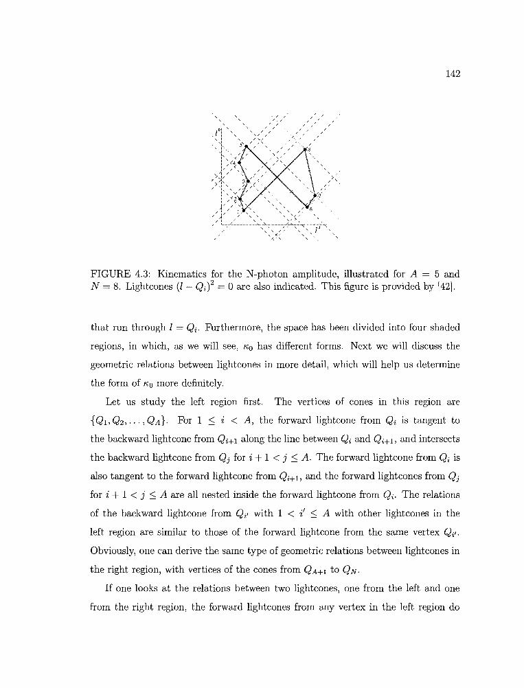
142
) .'
/ '/ '
/
/
,, ,, ,, ,, ,
/
/
// L ~: ~ ".: _._..:._'--, :,-.c- :.'"
" " / / ",'<;~ ',',
,)
FIGURE 4.3: Kinematics for the N-photon amplitude, illustrated for A = 5 andN = 8. Lightcones (I - Qd 2 = 0 are also indicated. This figure is provided by [42].
that run through I = Qi' FUrthermore, the space has been divided into four shaded
regions, in which, as we will see, "'0 has different forms. Next we will discuss the
geometric relations between lightcones in more detail, which will help us determine
the form of "'0 more definitely.
Let us study the left region first. The vertices of cones in this region are
{Ql, Q2, ... , QA}. For 1 ::; i < A, the forward lightcone from Q i is tangent to
the backward lightcone from Qi+l along the line between Qi and Qi+l, and intersects
the backward lightcone from Qj for i + 1 < j ::; A. The forward lightcone from Qi is
also tangent to the forward lightcone from Qi+l, and the forward lightcones from Qj
for i + 1 < j ::; A are all nested inside the forward lightcone from Qi. The relations
of the backward lightcone from Qi' with 1 < if ::; A with other lightcones in the
left region are similar to those of the forward lightcone from the same vertex Qi"
Obviously, one can derive the same type of geometric relations between lightcones in
the right region, with vertices of the cones from QA+l to QN.
If one looks at the relations between two lightcones, one from the left and one
from the right region, the forward lightcones from any vertex in the left region do
143
not intersect with the backward lightcones from any vertex in the right region. The
only exception is that the forward lightcone from Q1 is tangent to the backward cone
from QN along the line between Q1 and QN' Vice versa, the forward cones from
any vertex in the right region will not intersect with the backward lightcones from
any vertex in the left region, with the only exception of the forward cone from QA+1
being tangent to the backward cone from QA along the line from QA to QA+1'
There are no lightcone vertices at all either in the top region or the bottom region.
However, in the top region, the forward cones from any vertex in the left region will
intersect the forward cones from every vertex in the right region. Once again, the
exception is the forward cone from Q1 in the left region is tangent to the forward
cone from QN' In the same top region, the forward cones from any vertex in the
right region intersect the forward cones from every vertex in the left region, with the
exception that the forward cone from QA+1 is in fact tangent to the forward cone
from QA. For intersections in the bottom region, we can simply duplicate the above
analysis.
The picture of the lightcone configurations look very different when A = 1 or
A = N - 1. Fortunately, the above argument still holds in these two special cases.
To parameterize the four different regions, we choose a convenient set of coordinate
system and define the coordinates to be
x(l - QA+1) . P
p.p(l - Q1) . p
p.p (4.13)
Accordingly, the left region is x < 0 and x > 0; the right region is x > 0 and x < 0;
the top region is x > 0 and x > 0; the bottom region is x < 0 and x < o.
144
4.2.3 Double Parton Scattering
Until now we have seen collinear singularities and soft singularities, and have
concluded that they are in fact all integrable singularities because the powers of
zeros in the denominator could be lowered by corresponding numerator functions.
There could be one true singularity in the numerical integration, called double parton
scattering singularity, and it appears only if the line from Q1 to QN intersects the
line from QA to QA+1. A pinch singularity will sit right at such an intersection. Even
if the external momentum configuration does not exactly satisfy the above condition,
the two lines may still be close to intersecting, and the nearby region would cause
trouble to the numerical convergence of the integral.
In a real reacton where two photons scatter to produce more photons, the double
parton scattering will happen when the situation illustrated in Fig. 4.4 is true.
Generally, incoming photon N could split into a pair of off-shell electron and positron,
while the other incoming particle, photon A, could also split into a pair of off-shell
electron and positron. The electron from photon N could annhilate with the positron
from photon A and produce two or more external photons, and the positron from
photon N could also interact with the electron from photon A and produce two or
more external photons. Note that the reference frame can always boosted so that
neither of the two incoming photons has transverse momentum. Furthermore, we can
even choose a frame where the two incoming external photon are traveling on parallel
trajectories in opposite directions. One special case, as shown in Fig. 4.4, is the head
on collision of the initial photon pair, in which there exists one loop momentum to
make the splitting of photon N and the splitting of photon A both collinear, with
the two pairs of electrons and positrons all on shell, because the impact parameter
is now zero. Two collinear branchings at the same time could dramatically enhance
the cross section of the head-on collision, and thus contribute to a real divergence of
the integral. We can also easily prove that the double parton scattering singularity
exist if the transverse component PT of a subset (containing at least two photons) of

145
FIGURE 4.4: Physics picture of the double parton scattering. This figure is providedby [41].
the total external momentum vanishes in a frame where the incoming momentum are
pointing in the +z and -z direction. The amplitude can numerically be very large
when P~ «s. The PT test can be very useful in practical applications to crudely
evaluate the severity of the double parton scattering problem.
More precisely, one can find out how close the line between Q1 and QN is to the
line between QA and QA+1. If the two lines do intersect, apparently we would have
x = 0 and x = 0 for the intersecting point according to our earlier definition of x and
x, and there is no other point on the above two lines whose values of x and x can
vanish at the same time. However, if the two line do not intersection, there would
be exactly two points with a pair of zero x and x. We can find out the positions of
those two points by parameterizing the two lines using two additional parameters aj
and all, which are used to specify one arbitrary point on each of the line respectively.
The point on the line from Q1 to QN is called VI, and
(4.14)
146
It automatically has x = O. Using Eq. (4.13) and the definitions of P, P, if the x
value of point VI also vanishes, we must have
o (VI - QA+d· P
(-aIP+ QN - QA+d· P. (4.15)
One can therefore solve for aI and get an expression for point VI in terms of Qi, P and
P, which are all calculable based on the input of the diagram calculation. Similarly,
we can define
(4.16)
and solve for the only an that gives x = O. VI - Vn is a spacelike vector, and
the separation of the two points can be measured by the Lorentz invariant quantity
- (VI - vn)2. The smaller this separation is, more singular the nearby region would
be. One can denote the midpoint between VI and vn to be V,
V == (VI + vn) /2 . (4.17)
Naively this can be thought of as the most singular point. In our numerical program,
we choose V to be the origin of the coordinate system for I, although we shall not
assume this in the following discussion.
4.2.4 Deformation in All Four Regions
Now we shall propose a specific deformation by specifying the corresponding 4
vector 1);0 (I). As seen before, the contour eventually will deform into the complex
space by adding an imaginary part, i/), (l), and /), (I) is proportional to /),0. The
question of how far to deform the contour will be answered later. First we shall
present a general formula for /),0 (I), and the coefficients of different terms included
147
in the formula will then be given. Then it will be shown that this method does yield
a map of I'l:o and the integral contour can be deformed in the right direction required
by the +iO prescription everywhere in the space of l.
Define
N
I'l:o = - ~ cj(l- Qj) + c+ (P + P) - c_ (P + P) , (4.18)j=1
where coefficients Cj, c+ and c_ are all non-negative functions of l, and the lower
index j runs from 1 to N. Different terms are responsible for the deformations in the
four shaded regions indicated in Fig. 4.3, and they are carefully turned on and off as
one integrates over l along the contour.
For the generic case 1 < A < N - 1, we choose the coefficients to be
Cj = h_(l- Qj-d h+(l - Qj+d h_(l- QN)
x h+(l- QA+dg(l) j E {2, ... ,A-1},
Cj = h_(l- Qj-d h+(l- Qj+d h_(l - QA)
Xh+(l-Ql)g(l) jE{A+2, ... ,N-1},
Cl = h+(l - Q2) h_(l- QN-l) h+(l - QA+d g(l) ,
CA = h_(l- QA-d h+(l- QA+2) h_(l - QN) g(l) ,
CA+l = h+(l- QA+2) h_(l- QA-l) h+(l - Ql) g(l) ,
CN = h_(l- QN-d h+(l- Q2) h_(l - QA) g(l) ,
c+ = h_(l- QA) h_(l- QN)
x (x+x)e(x+x > 0) g-(l),
c_ = h+(l- Ql) h+(l- QA+d
x [-(x + x)] e(x + x < 0) g+(l) .
(4.19)
The functions h± (l), g± (l) and 9 (l) control the boundaries of regions for nonzero Cj,
148
C+ and C_, and will be defined below. For the special case A = 1, the definitions of
coefficients are a bit different,
Cj = h_(l- Qj-l) h+(l- Qj+d h_(l- Ql)
x h+(l - Ql) g(l) j E {3, ... ,N - I} ,
Cl = h_(l- QN-d h+(l- Q3) g(l) ,
C2 = h+(l- Q3) h+(l- Ql) g(l) ,
CN = h_(l- QN-l) h_(l- Ql) g(l) ,
c+ = h_(l- QN) (x + x) e(x + x> 0) g-(l) ,
c_ = h+(l - Q2) [-(x + x)] e(x + x < 0) g+(l) .
For the other special case A = N - 1,
Cj = h_(l- Qj-l) h+(l- Qj+l) h_(l- QN)
x h+(l- QN)g(l) j E {2, ... ,N - 2},
Cl = h+(l - Q2) h+(l- QN) g(l) ,
CN-l = h_(l- QN-2) h_(l- QN) g(l) ,
CN = h+(l- Q2) h_(l- QN-2) g(l) ,
c+ = h_(l- QN-l) (x + x) e(x + x> 0) g-(l) ,
c_ = h+(l- Ql) [-(x + x)] e(x + x < 0) g+(l) .
(4.20)
(4.21)
The factors h± (l - Qi) contained in Cj are functions of momentum l. For the purpose
of obeying +iO prescription, we want h+ to vanish only in the forward lightcone from
Qi, and want h_ to vanish only in the backward lightcone from Qi' The above
requirement can be satisfied if
(4.22)
(4.23)
149
and
h (k) = _ (Ikl- Ek )2 e(Ek < Ikl) .+ (Ikl - E k )2 + M'f
In the above definitions, E k and k are the energy and the spatial components of
the 4-vector k. Constructed as such, it can be easily proved that h+ (k) = 0 in the
forward lightcone from i = 0 and h_ (k) = 0 in the backward lightcone from i = O.
The magnitude of this function is affected by our choice for the parameter MI. In
our numerical program, the default value is M 1 = 0.05 (P . P) 1/2.
Factor 9 (i) is also included in the definition of Cj, and it is used to make sure the
contour deformation is relatively larger near the possible double parton scattering
singularity compared to those region far away from this singularity. It is in fact quite
rare to have a configuration of the external momentum that allows the presence of
double parton singularity, but the numerical convergence in the region near the point
v as we defined above is usually marginal. So we want to deform the contour away
from v as much as possible. The form of 9 (l) we adopt is defined to be
(i) - 1'1 Mi (4 24)9 - (iO _ VO)2 + (l- v)2 + Mi .
The dimensionless parameter I' determines the magnitude of 9 (i) right at v, and is
by default set to be 0.7 in our numerical program. The other parameter M2 is by
default set to be M2 = (P . 15) 1/2, and it affects the size of the deformation in regions
further away from the double parton scattering region.
The coefficient C+ includes a factor 9_ (i) and the coefficient c- includes a factor
9+ (l). If taking the top region as an example, we want the contour deformation to be
large on the forward lightcones and the spacelike intersections of forward lightcones
in the top region, and we want the deformation to be small when the contour is far
away from any singular region. This can be roughly satisfied by forcing the magnitude
of "'0 (i) to maximize on the surface of the upper branch of a hyperbola, with the
(4.25)
150
forward lightcone from the point v as its asymptotes, since most forward lightcones
from vertices in the left and right region will be near such a hyperbola. Therefore, we
find it could be helpful to let c+, which regulates the deformation in the top region,
to include the factor
(l) = "Iz9- 1 + (1- E/w)z '
where "Iz is a dimensionless parameter that affects the size of the contour deformation
near all forward lightcones. The parameter E and ware defined as
(4.26)
(4.27)
in which the parameter M3 has the dimension of mass and impacts when to maximize
c+" We set the default values of "Iz and M3 to be 1 and (p. P) l/Z in our numerical
program. Similarly, we choose the factor 9+ (l) in c- to be
(l) - "Iz9+ - 1 + (1 + E / w)z ,
with the same definitions for "Iz, E and was above. This way the deformation will also
approximately be large near the singular points and surfaces in the bottom region
and gradually decreases as the contour moves to domains without any cones.
Next, we shall first introduce some useful notations for the lightcones, and then
we will try to find out whether the general formula for 1);0 defined in Eq. (4.18) is
really able to yield the correct deformation near singularities by tracking the values
of 1);0 • (l - Qi). The generic case will be studied before the special case with A = 1
or A = N-1.
151
4.2.5 Notations for Cones
In order to make the later analysis more compact, we will name different parts of
a light cone, and use the cone from Qi as an example. The forward lightcone will be
denoted by C+ (Qi),
(4.28)
and the forward lightcone plus its interior will be denoted by C+,
(4.29)
The dot products of (I - Qi) and (p + P) are positive in the above two cases because
the two factors are both timelike vectors pointing in the same time direction. We
also denote the backward lightcone from Qi,
(4.30)
by C_ (Qi), and denote the backward lightcone plus its interior,
(4.31)
The dot products are now negative because the two factors are timelike vectors
pointing in the opposite time directions.
4.2.6 The Coefficients for 2 :s A :s N - 2
4.2.6.1 The Coefficients Cj for j E {2,'" ,A - 1}
We can have "'0' (I - Qi) 2: 0 for I on the lightcone from any Qi as long as every
single term in the definition of "'0 can have a non-negative dot product with the same
152
factor (I - Qi)· Let us talk about Cj with j E {2,··· ,A - I} first. We define the
term in ""0 that contains Cj to be
For I E C± (Qi) with any i other than j, we find the product
(4.32)
-Cj(l - Qi)2 + Cj(Qj - Qi) . (l- Qi)
Cj(Qj - Qi) . (I - Qi) . (4.33)
We first consider the case of j < i ~ A where Qj E C_ (Qi). Therefore, for
I E C_ (Qi) we would have ""j" (I - Qi) as desired since Cj is chosen to be non-negative
already. However, for I E C+ (Qi) the same dot product will never be greater than
zero. As a result, we have to make Cj vanish for I E C+ (Qi) in order to make the
product non-negative for all I on the cone from Qi. It is true that within the given
range of i and j in this particular case we always have C+ (Qi) C C+ (Qj+d. We can
then include the factor h+ (I - Qj+d in Cj so that it will vanish for I E C+ (Qi).
Similarly, if we consider the case where 1 ~ i < j we can get Qj E C+ (Qi) for any
j E {2,··· ,A - I}. It is ensured that ""j. (l- Qi) ~ 0 for any IE C+ (Qi), but again
the same dot product has the wrong sign for I E C_ (Qi), and thus Cj has to vanish
on the backward lightcone from Qi. Using the nesting relation C_ (Qi) C C_ (Qj-l),
we find we can acquire the correct sign by including a factor of lL (I - Qj-d in the
coefficient Cj.
So far we have only studied the cases where i ~ A. When A + 1 ~ i ~ N, the
two vertices Qi and Qj would be spacelike separated, and ""j . (1- Qi) can be either
positive or negative for I anywhere on the lightcone from Qi, based on Eq.(4.33).
Therefore, in order to make the dot product non-negative, we force Cj to vanish for
any I E C± (Qi). Since it is true for any i E [A + 1, N] that C+ (Qi) C C+ (QA+l)
and C_ (Qi) C C_ (QN), we include factor h+ (1- QA+l) and factor lL (l- QN) in
153
the definition of Cj. The factor 9 (l) is also included because we want to turn off the
deformation gradually when lO and fare large.
4.2.6.2 The Coefficients Cj for j = A
In this case, when i < j = A, the dot product K,j . (l - Qi) is again positive for
l E C+ (Qi) and negative for l E C_ (Qi) based on Eq. (4.33), and thus we still want
the factor h_ (l - Qj -1) in Cj (or CA). However, unlike j < A, there is no i that
could be greater than j = A and not larger than A, so we do not need the factor
h+ (l - Qj+1) in Cj any more.
For A + 2 ::; i ::; N, Qi and QA are spacelike, and /'\;A . (l - Qi) can be either
positive or negative for l E C± (Qi). The coefficient CA needs to vanish on the
lightcones from such Qi to generate the correct deformation. The nesting relations
now become C+ (Qi) C C+ (QA+2) and C_ (Qi) C C_ (QN). Accordingly, we include
the factor h+ (l - QA+2) and the factor h_ (l - QN) in CA.
We have not covered the case of i = A + 1 yet. Obviously QA and QA+1 are
lightlike, and QA E C+ (QA+l). The condition K,j . (l - Qi) 2: 0 are always satisfied
for any l E C+ (Qi) when i = A + 1 and j = A. For l E C_ (l - QA+d, the dot
product carries the "wrong sign", and CA has to vanish on the backward cone from
QA+1· We notice that C_ (QA+d C C~ (QN). The factor h_ (l- QN) that we have
already included in CA will therefore ensure that CA goes to zero for l E Q- (QA+d.
4.2.6.3 The Coefficients Cj for j = 1
Just as the analysis we have done for CA, the definition of C1 is similar to Cj for
1 < j < A - 1 but not identical. We do not need to include the factor h_ (l - Qj-d
because there is no Qi that satisfies 1 < i ::; j = 1 and we are automatically free of
some problems in which /'\;j • (l - Qi) has the "wrong" sign. We can force C1 to vanish
for l E C± (Qi) with A + 1 ::; i ::; N - 1 by putting in the factor h+ (l - QA+1) and
the factor h_ (l - QN-d.
154
4.2.6.4 The Coefficients Cj for j E {A + 1, ... ,N}
The coefficients Cj for A + 1 :::; j :::; N can be defined in the same way as we define
those coefficients Cj for 1 :::; j :::; A.
4.2.6.5 The Coefficient c+
We have defined a group of coefficients Cj for j E {I, ... , N}, and have proved
the corresponding "'j can yield "'j' (l - Qi) ~ 0 for any l E C± (Qi), where the index
i can be any integer between 1 and N. Moreover, one can show, in a straightforward
but tedious way, that L "'j . (l - Qi) > 0 for all l E C± (Qi) except for those
loop momentum on the pinched singularities in the left and right region in Fig. 4.3.
This is exactly what we want, because in order to have better control over the
numerical convergence of the whole integral, we need the contour to be deformed
from a singularity whenever it is possible. However, we have not achieved the same
objective yet in a large part of the top and bottom region with the collection of "'j,
e.g., L"'j = 0 for l on the intersection of C+ (Q2) and C+ (QA+2)' In fact, "'j are
mostly turned off in the top and bottom region because "'j' (l - Qi) could be negative
on the spacelike intersection of lightcones, as we discussed earlier.
Fortunately, this problem can be easily resolved by putting in a new term "'+to the imaginary part of £, and "'+ . (l - Qi) > 0 is always true for l E C+ (Qi) as
long as "'+ is timelike and points to the positive direction in time. We thus choose
"'+ ex: (p + P). The formal definition of this new term is
(4.34)
Obviously "'+ . (l- Qi) will have the "wrong" sign for l E C_ (Qi), and we need
to make sure c+ vanishes for those l. This requirement can be met by including
the factor h_ (l- QA) and the factor h_ (l- QN) since all other backward cones are
nested inside the backward cone from either QA or QN'

- -----------------
155
In practice, not only do we want to have nonzero deformation at the singularities,
but we also want to suppress the deformation when the contour is not near any
singularity. For this purpose, factors (x + x) e(x + x > 0) and 9_ (l) are included
when defining c+. As we argued before, the function 9_ (l) approaches approximately
1 near the forward lightcones in the top region, and x + x will grow with l along the
cones. The outcome is that the contour can be deformed significantly away from
the forward lightcones when l moves away from the double parton scattering region.
However, if the spatial component lis fixed, (x + x) 9_ (l) will decrease to zero when
its a-component gets bigger, which effectively turns off the deformation.
4.2.6.6 The Coefficient c_
Similar to what we have done to the coefficient c+ in the top region, we want to
add a new term /"'- to /\'0 so that /\, . (l - Qi) is positive for any l E C_ (Qi) in the
bottom region. Once again this can be easily achieved as long as /\,_ is timelike and
points to the negative direction in time. In particular, we can define
(4.35)
This same /\,_ would yield the "wrong" sign for /\,_. (l - Qi) on the forward lightcones
from any of the Qi, and thus c_ has to be turned off on all forward cones. This can
be ensured by including in the definition of c_ the factor h+ (l - Qd and the factor
h+ (l - QA+1), because all other forward cones are nested inside the forward cone
from either Q1 or QA+1. We also put in factors - (x + x) e(x + x < 0) and 9+ to
control the deformation in the bottom region.
4.2.7 The Coefficients for A = 1
When A = 1, the coefficients that appear m the definition of /\'0 need to be
specified slightly differently from the generic case where 2 :s A :S N - 1.

156
The geometric arrangements of the lightcones cones from Qj for
J E {3, ... , N - I} is the same as those of the lightcones from vertices in the
right region of the generic case. Therefore, the definitions of Cj completely follows
those of Cj for 3 :s; j :s; N - 1 in the generic case.
On the other hand, the coefficients CI, C2, CN, c+ and Cj need to be modified. Let us
start with CI. For K, I ex: - (I - QI), it points in the right direction for I E C+ (Q2) and
IE C_ (QN), but it points in the "wrong" direction for IE C_ (Q2) and IE C+ (QN).
Furthermore, K,l . (I - Qi) for i E {3, ... , N - I} can be either positive or negative.
To summarize, we want CI to vanish for I on all forward lightcones nested in the
forward cone from Q3 and for I on all backward cones nested inside the backward
cone from QN-I' The above requirements on CI can be realized by including factors
h+ (I - Q3) and h_ (I - QN-I).
The analysis for the coefficient C2 is similar. The vector K,2 points in the correct
direction for I on backward cones from all Qi except for Q2 itself, because the cone
from Q2 is nested inside any other backward cone in the problem. Accordingly, K,2
will point in the "wrong" direction for I on forward cones from all Qi except for Qi'
We thus require C2 to vanish on all the forward cones except for that from Q2' It is
achieved by including in C2 factors h+ (I - Ql) and h+ (I - Q3)'
Analogously to C2, CN can point in the right direction for all I by including in it
factors h_ (I - Qd and h_ (I - QN-I).
For c+, the vector K,+ ex: (p + P) obviously points in the right direction for I E
C+ (Qi) with any valid i choice, and points in the "wrong" direction for I E C_ (Qi)
with all valid i choice. We have a very convenient nesting relation to make use of when
A = 1 because all backward cones are nested inside the one from QN, and that means,
compared to the generic case, we only need to include in c+ the factor h_ (I - QN)
in order to make c+ vanish for I on all backward lightcones. Factors (x + x) e(x + x)
and g_ (I) is again used to control the relative size of the deformation in different sub
regions. The construction for c_ is similar to that of c+.
157
4.2.8 The Coefficients for A = N
The construction of the coefficients in the definition of lio follows the same logic
as that used in the special case of A = 1.
4.2.9 Size of the Deformation
We have so far determined the directions of the vector Ii everywhere in the space
of l by specifying lio and its coefficients as functions of l. As defined before,
(4.36)
and the real scalar factor A(l) controls the size of the deformation together with
lio. To stick to the +iO prescription, we need to ensure the integrand does not run
into any singularity as A (l) is increased from zero to its final value, otherwise the
modified contour might enclose different poles and thus have different residues from
the original contour. It is trivial when A(l) is infinitesimally small, because under the
guidance of lio the contour has already started to deform away from the non-pinched
singularities in the correct direction near the original route. However, the practical
A (l) should be as large as possible. Being too close to the singularities will undermine
the numerical convergence of the integral. On the other hand, one would guess A(l)
cannot be arbitrarily big, because for certain values of A it could be true that
(l- Qi + iA (l) lio (l))2 = 0 (4.37)
for some l away from the original singularities, while lio (l) . (l - Qi) > 0 for l near
those non-pinched singularities. It is also possible that when the contour get deformed
away from one cone, Qi, it might end up coming across the singularity near another
cone, Qj, which means
(l- Qj + iA (l) lio (l))2 = 0 (4.38)
158
The above analysis implies that we should find out the rules about how far the
contour can be deformed. The upper limit for A(i) needs to be set. In order to
resolve this problem, it is helpful to first see where the new singularities could be in
terms of the corresponding values of A(i). We can better formulate this subject by
requiring the maximum value, Af (i), to be the minimum of a number, Ai (i), defined
for each propagator, a universal choice, Ao (i), to be determined later, and a constant
number, Ac , whose default value is 1 in our numerical program:
Af (i) = Min [Min {Ai (in, Ao (i) ,Ac] . (4.39)
We first determine what Ai should be for each propagator. The new singularity
related to the cone from Qi appears when
The root of this quadratic equation of A is
A= -; {i K;O • (i - Qi)K;O
± VK;6 (i - Qi)2 - [K;O . (i - Qi)j2 }
(4.40)
(4.41)
We can see that since the solution for A(i) can be either real or complex, thus
the new singularity does not necessarily exist. The poles can have real parts when
[K;o . (i - QiW < K;~ (i - Qi?' but they will not be able to get near the real axis
unless [K;O' (i - QiW « K;~ (i - Q.i? are satisfied. In that case, one of two poles of A
can have a finite positive real part and the imaginary part of the same pole almost
vanishes, which means the contour can get very close to this pole as one increases A.
The special situation is when K;O • (i - Qi) = 0 and thus the same pole sits right on
the positive real axis. The absolute value of this pole would be

IAI =
1:61 V["'o . (l - Qi)]2 + ["'6 (l - Qi)2 - ("'0' (l - Qi))2]
(l - Qi)2",2o
159
(4.42)
Obviously we can avoid being too close to or even encountering this new singularity
easily by defining the corresponding Ai to be smaller than the absolute value of this
real pole. We will talk about the specific form for Ai later.
The poles can be purely imaginary when "'6 (l - Q'i? < ["'0' (l - QiW, and the
exact expressions for them will be
A = ~ {"'D. (l - Qi)"'0
± V["'o . (l - Qi)]2 - "'6 (l - Qi)2 }(4.43)
As we increase A from zero along the positive real axis, the contour will never get
close to any new singularity since the poles are both on the imaginary axis. Given
this, one would certainly want to set Ai to be as large as possible so that the contour
can be far away from the original singularity. However, there are still restrictions on
what one can actually use for Ai in this region of l. The most important constraint
comes from the requirement that the Jacobian determinant present in Eq. (4.7) needs
to be small. If the change in '" as we vary l is too sharp, or equivalently, if the gradient
of '" with respect to l is too large or even singular, the numerical convergence of the
integral in Eq. (4.7) will remain marginal due to a large or even singular Jacobian,
even if we have deformed the contour well away from the singularities. To fix this,
we have to make sure that Af is continuous across all possible boundaries at all times
and that the gradient of Af is never too large. Next we will discuss the construction
of Ai (l) and AD (l) in more details and see how the above criteria can be satisfied.

160
For the purpose of defining Ai, we will first divide the l space into three different
regions. The first region has
(4.44)
and it encloses all the sub regions where one of the two A poles in Eq. (4.41) can be
either close or right on the positive real axis of A. Therefore, we need a Ai that is small
enough so that the contour will not come across any new singularities. Particularly,
we can choose Ai to be only half of the absolute value of the poles,
A2 = /1;6(l- Qi)2~ (2/1;6)2
for 2[/1;0· (l - QiW < /1;6 (l - Qi)2
The second region is where
(4.45)
(4.46)
Note that at the boundary between region I and region II Ai has to be continuous.
We can define
A~ = 4[/1;0· (l - QiW - /1;6(l - Qi)2~ (2/1;5)2
for 0 < /1;6 (l - Qi)2 < 2[/1;0· (l - QiW ,
(4.47)
which does match the definition for Ai when /1;6 (l- Qi)2 = 2[/1;0· (l- Qi)]2. The third
region, which covers the rest of the l space, is when
(4.48)
and accordingly, one can define Ai in this region as well so that it can match the
definition for Ai in region II at the boundary, where /1;6 (l - Qi)2 = O. This motivates
us to choose in the third region that
·_----- -------------
161
2 4[K:o· (l - Qi)]2 - 2K:6(l - Qi)2.\ = (2K:5)2
for K:6 (l - Qi)2 < 0 .
(4.49)
Note that the above definitions for Ai are smooth functions of l almost everywhere,
except when the denominator K:6 = o. It means the gradient of Ai, hence the gradient
of K: (l), should be finite whenever K:o is not lightlike. On the other hand, the 4-vector
K:o cannot be lightlike unless its argument l is on the collinear lines. If l does sit
on the collinear singularities along one of the two lines l = Qi + Z(Qi+l - Qi) and
l = Qi + Z(Qi-l - Qi) that meet at l = Qi, both the numerator and the denominator
of Ai in any of the three regions will be zero. Naively it could easily be true that the
resulting Ai is also zero and gets picked to be AI since it is the smallest among AO' Ac
and min [Ai]. At the same time the gradient of this Ai, and hence the corresponding•
K:, could be singular. We do not want this to happen, and thus need to discuss in
more details about the values of Ai near the collinear lines we have just mentioned.
However, for l on all other collinear singularities that are not included above, it does
not matter if the gradient of Ai (l) is singular or not, because for those points the
numerator of Ai (l) would not be zero. Therefore, Ai will be infinitely large and cannot
be chosen to be AI, the upper limit for A(l) at that point.
The optimal scenario for this issue would be that there actually is a positive
and finite minimum value that Ai can ever get as small as. If it were true, then we
could choose a smooth function of l, AO (l), which will always be smaller than this
same minimum value for Ai near the collinear singularities closest to Qi. This way
the gradient of AI will never be singular, even though in those regions that we are
now considering the gradient of Ai can be very singular. To see whether this scenario
applies, we need to find out what the expressions for Ai will become near the collinear
singularities. We first rewrite the definition for K:o as
N
K;O = - L Cj(l- Qj) + C+(P + P) - c_(P + P)j=l
where
N
C= LCj ,j=l
N
I4 = LCj(Qj - Qd + c+(P + P) - c_(P + P)j=l
Under this new notation, we can derive that
and another term that also appears in the definition of Ai,
162
(4.50)
(4.51)
(4.52)
(4.53)
The third term (also the last term), (l - Qi)2, included in Ai can be related to the
other two terms by eliminating (l - Qi) . Ri from the above two equations, and then
one can obtain
(4.54)
Through tedious but straightforward analysis, we can find out that as l moves towards
the collinear singularities closest to Qi, the term R; tends to behave like [(l _ Qi)2] 2,
and approaches 0 very fast. The consequence of this observation is R; can therefore be
neglected in this region since it is a higher order term in the small quantity (l - Qi)2
compared to K;& and K;O • (l - Q)i). After making this approximation, we can have
163
(4.55)
If we square Eq. (4.55) and divide both sides of the equation by 2, we shall get
2["';0' (l - QiW ~ ,.,;6(l- Qi)2
C2[ 2]2 1 [2] 2+ "2 (l - Qi) + 2C2 "';0
> ,.,;6(l - Qi)2 ,
(4.56)
which means l would never be in the first region defined above when it is very
close to the collinear singularities along the two lines l = Qi + Z(Qi+l - Qi) and
l = Qi + z(Qi-l - Qi) that meet at l = Qi' However, the possibility of l being
in the other two regions cannot be ruled out, and it will depend on the sign of
,.,;6 (l - Qi)2 whether l belongs to region II or III. Nevertheless, we can figure out
what the global lower limit of Ai is by studying the lower limits of the same function
in two regions separately. In region II, if we replace "';0 . (l - Qi) in Eq. (4.47) by
using the approximated relation worked out in Eq. (4.55), we can conclude
(4.57)
Note that in the second line in the above equation, the first term is always non
negative, and it can vanish only when l approaches the boundary between region II
and III which is ,.,;6 (l- Qi)2 = O. Similarly, in region III we can replace "';0' (l- Qi)
in Eq. (4.49) using Eq. (4.55), we will find
(4.58)

(4.59)
(4.60)
164
Again, A~ can approach 1/4C2 only when l is near the boundary between region II
and III. In summary, for any l near the collinear singularities along the lines that
meet at l = Qi, it is always true that
1A·>• 2C
Since we want continuous Af everywhere in the l space, including the region near
collinear singularities, we can define
1Ao(l) = 4 C(l) ,
so that Af will be set to be the same smooth function of l accross all collinear
singularities.
4.3 Numerical Results
We have developed a computer program that incorporates the contour deforming
mechanism described in this thesis, using C++. The program is designed to calculate
the matrix element M by evaluating the integral presented in Eq. (4.7). For the
corresponding virtual loop Feynman diagram with N external photons, all N external
momentum Pi and photon polarizations Ei will be given as inputs before the computer
code is executed. Among them, 2 are incoming photons and the rest are outgoing.
To start with, we choose PI and P2 to be the momentum of the two incoming photons,
and let their transverse components vanish. However, we are interested in more than
just one diagram. Our goal is to compute the amplitude of 2 photons with fixed
momentum scattering to produce (N - 2) other photons also with pre-determined
momentum, regardless of their relative positions around the virtual loop in the graph.
As a result, for N photons we need to consider all of the non-cyclic permutations of
initial labeling of photon legs. There are (N - I)! such permutations in total. After
a permutation, as illustrated in Fig. 4.3, photon A and photon N will be initialized
165
to have the incoming momentum and polarizations. The amplitude at interest will
finally be acquired by summing the graphs over all possible permutations.
We will now pick an observable 0 that can best characterize our numerical
calculation. We specify the helicities in a form {hI, hz, .. . , hN }, with hI and hz
being the helicity of incoming photons. According to our notation, hI and hz are
actually the negative of physical polarizations because we have defined all external
momentum to be outgoing for convenience. For a given set of helicities for the external
photons, the phase of the matrix element M actually differs for different conventions
for the photon polarization vector. In practice, this phase does not have any effect
since we only concern about the absolute value of the scattering amplitude, IMI. We
can choose any convention for the polarization vector tp. (k, s) before squaring the
amplitude, and the final result will be proportional to IMI and will not depend on
where we start with. Moreover, we want to make 0 dimensionless, since we care more
about the interaction between the external momentum plus helicity configurations
and the final amplitudes. As a result, we need to divide 1M I by (VS) 4-N, where
VS is the center-of-mass energy of the initial photon pair. Applying the same logic,
we also want to remove the effects brought by the coupling constant by including a
factor of 1/aN/Z
. As a result, we want to show
(4.61)
in our subsequent plots.
In the computer code, we compute M in a Monte Carlo style, and we deform
the contour away from its original path in the complex plane. To achieve optimal
numerical convergence, we adopt K different methods of importance sampling in
regions where two or more lightcones intersect so that more points can be used
where bigger fluctuations are expected. The probability for the code to execute
method i is ai, for which points are sampled according to the distribution 9i (l). It
166
is straightforward to see that the value of the original integral will be retained as we
have
(4.62)
K
where L 0:i = 1. The form of the distribution 9i (l) depends on how lightconesi
intersect. Among the (N - I)! graphs pertaining to the same scattering amplitude,
some of them are more singular when the impact parameter b is smaller, because
those graphs will have a more severe problem of double parton scattering. So instead
of assigning equal weights to all graphs, we put more weights in those more singular
graphs when summing them over permutations. We have documented some sampling
methods at [45]. In the rest of this section we will display the numerical results of
N = 6 and N = 8 for several helicity configurations, and then compare them with
those using the Feynman parameter method.
4.3.1 N = 6
We choose to compute a group of scattering amplitudes with six photons that
are all located along an one-dimensional curve in the space of external momentum.
First an initial set of external momentum is given, in which momentum of the two
incoming photons, PI and P2, do not have any transverse component. In our case, we
let PI point in the - z direction so that the physical direction of photon 1 points in
the +z direction according to our notation, while we let P2 point in the +z direction.
The starting point of outgoing momentum used in our computer code is arbitrarily
chosen to be
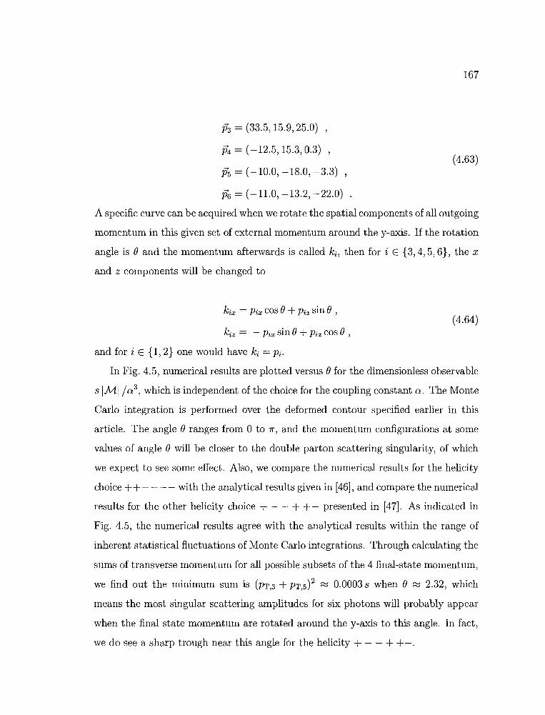
(4.63)
(4.64)
167
fa = (33.5,15.9,25.0) ,
P4 = (-12.5,15.3,0.3) ,
P5 = (-10.0, -18.0, -3.3) ,
ik = (-11.0, -13.2, -22.0) .
A specific curve can be acquired when we rotate the spatial components of all outgoing
momentum in this given set of external momentum around the y-axis. If the rotation
angle is () and the momentum afterwards is called ki , then for i E {3, 4, 5, 6}, the x
and z components will be changed to
k ix = Pix cos () + Piz sin () ,
k iz = - Pix sin () + Piz cos () ,
and for i E {1,2} one would have k i = Pi.
In Fig. 4.5, numerical results are plotted versus () for the dimensionless observable
s 1M I / (i, which is independent of the choice for the coupling constant 0:. The Monte
Carlo integration is performed over the deformed contour specified earlier in this
article. The angle () ranges from 0 to 1r, and the momentum configurations at some
values of angle () will be closer to the double parton scattering singularity, of which
we expect to see some effect. Also, we compare the numerical results for the helicity
choice ++ - - - - with the analytical results given in [46], and compare the numerical
results for the other helicity choice + - - + +- presented in [47]. As indicated in
Fig. 4.5, the numerical results agree with the analytical results within the range of
inherent statistical fluctuations of Monte Carlo integrations. Through calculating the
sums of transverse momentum for all possible subsets of the 4 final-state momentum,
we find out the minimum sum is (PT,3 + PT,5)2 ~ 0.0003 s when () ~ 2.32, which
means the most singular scattering amplitudes for six photons will probably appear
when the final state momentum are rotated around the y-axis to this angle. In fact,
we do see a sharp trough near this angle for the helicity + - - + +-.
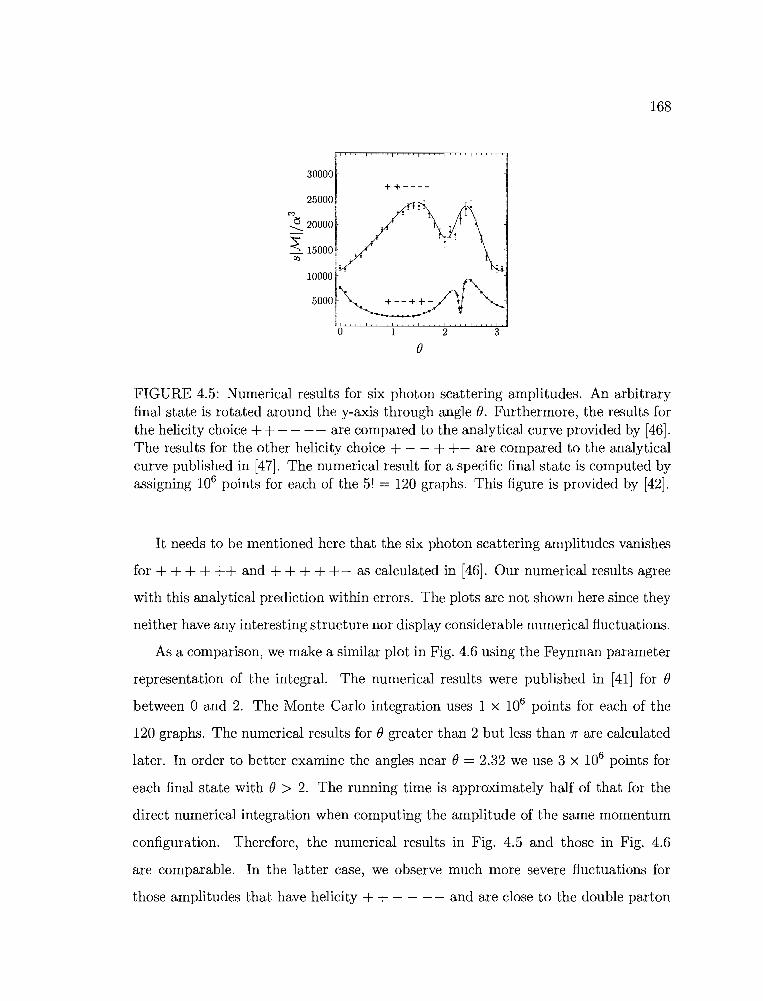
168
30000+ + ----
250000')
-2. 20000
:< 15000'"
10000
5000 +--++-
o()
2 3
FIGURE 4.5: Numerical results for six photon scattering amplitudes. An arbitraryfinal state is rotated around the y-axis through angle e. Furthermore, the results forthe helicity choice ++- - - - are compared to the analytical curve provided by [46].The results for the other helicity choice + - - ++- are compared to the analyticalcurve published in [47]. The numerical result for a specific final state is computed byassigning 106 points for each of the 5! = 120 graphs. This figure is provided by [42].
It needs to be mentioned here that the six photon scattering amplitudes vanishes
for + ++ + ++ and + + + ++- as calculated in [46]. Our numerical results agree
with this analytical prediction within errors. The plots are not shown here since they
neither have any interesting structure nor display considerable numerical fluctuations.
As a comparison, we make a similar plot in Fig. 4.6 using the Feynman parameter
representation of the integral. The numerical results were published in [41] for ebetween 0 and 2. The Monte Carlo integration uses 1 x 10⁶ points for each of the
120 graphs. The numerical results for egreater than 2 but less than 11' are calculated
later. In order to better examine the angles near e= 2.32 we use 3 x 10⁶ points for
each final state with e> 2. The running time is approximately half of that for the
direct numerical integration when computing the amplitude of the same momentum
configuration. Therefore, the numerical results in Fig. 4.5 and those in Fig. 4.6
are comparable. In the latter case, we observe much more severe fluctuations for
those amplitudes that have helicity + + - - - - and are close to the double parton
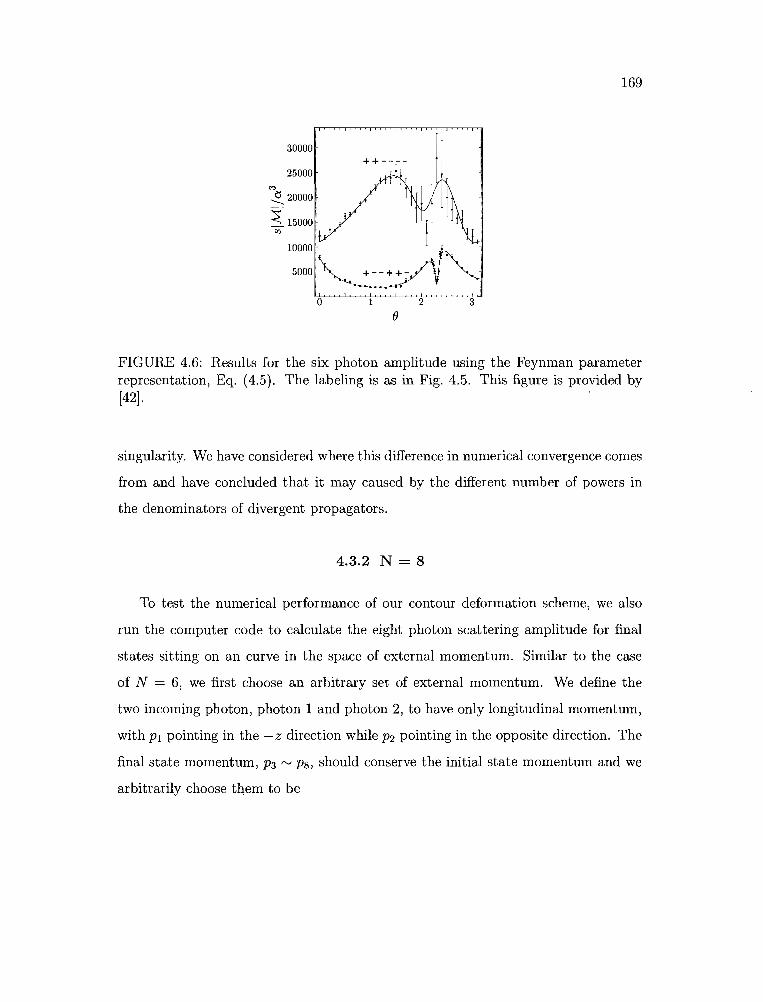
169
30000
25000M
~ 20000
<15000
'"
o(j
2 3
FIGURE 4.6: Results for the six photon amplitude using the Feynman parameterrepresentation, Eq. (4.5). The labeling is as in Fig. 4.5. This figure is provided by[42].
singularity. We have considered where this difference in numerical convergence comes
from and have concluded that it may caused by the different number of powers in
the denominators of divergent propagators.
4.3.2 N = 8
To test the numerical performance of our contour deformation scheme, we also
run the computer code to calculate the eight photon scattering amplitude for final
states sitting on an curve in the space of external momentum. Similar to the case
of N = 6, we first choose an arbitrary set of external momentum. We define the
two incoming photon, photon 1 and photon 2, to have only longitudinal momentum,
with PI pointing in the -z direction while P2 pointing in the opposite direction. The
final state momentum, P3 rv Ps, should conserve the initial state momentum and we
arbitrarily choose them to be
o()
2 3
170
FIGURE 4.7: Numerical results for the eight photon amplitude. The points forwhich amplitudes are calculated are acquired by rotating an arbitrary set of finalstate momentum around the y-axis through angle e. For comparison, the analyticalresults of [46] are also presented in the same plot. We use 2 x 10⁵ points for each ofthe 7! = 5040 graphs, except that we use four times more points, 1 x 10⁶ points, fore= 2.0 and e= 2.4 because t.he external momentum configurations are closer to thedouble parton scattering singularity for those two sets of momentum. This figure isprovided by [42].
P3 = (33.5,5.9,25.0) ,
i4 = (1.5,24.3,0.3) ,
iJs=(-19.1,-35.1,-3.3) ,
fie, = (28.2, -6.6,8.2) ,
ih = (-12.2, -8.6,8.2) ,
Ps = (-31.9,20.1, -38.4)
(4.65)
One can produce the entire curve by rotating the final state momentum given above
around the y-axis through angle e. We are again interested in e in the range from 0
to Jr.
We follow the same rules that have been devised to deform the contour for N =6 and compute a few different amplitudes for N = 8 whose external momentum
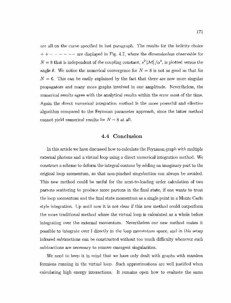
171
are all on the curve specified in last paragraph. The results for the helicity choice
+ + - - - - -- are displayed in Fig. 4.7, where the dimensionless observable for
N = 8 that is independent of the coupling constant, 82 1MI /a4
, is plotted versus the
angle e. We notice the numerical convergence for N = 8 is not as good as that for
N = 6. This can be easily explained by the fact that there are now more singular
propagators and many more graphs involved in one amplitude. Nevertheless, the
numerical results agree with the analytical results within the error most of the time.
Again the direct numerical integration method is the more powerful and effective
algorithm compared to the Feynman parameter approach, since the latter method
cannot yield numerical results for N = 8 at all.
4.4 Conclusion
In this article we have discussed how to calculate the Feynman graph with multiple
external photons and a virtual loop using a direct numerical integration method. We
construct a scheme to deform the integral contour by adding an imaginary part to the
original loop momentum, so that non-pinched singularities can always be avoided.
This new method could be useful for the next-to-Ieading order calculation of two
partons scattering to produce more partons in the final state, if one wants to treat
the loop momentum and the final state momentum as a single point in a Monte Carlo
style integration. Up until now it is not clear if this new method could outperform
the more traditional method where the virtual loop is calculated as a whole before
integrating over the external momentum. Nevertheless our new method makes it
possible to integrate over l directly in the loop momentum space, and in this setup
infrared subtractions can be constructed without too much difficulty whenever such
subtractions are necessary to remove emergent singularities.
We need to keep it in mind that we have only dealt with graphs with massless
fermions running in the virtual loop. Such approximations are well justified when
calculating high energy interactions. It remains open how to evaluate the same
172
scattering amplitudes but with massive fermion loop. The surface on which the
denominator of such a propagator vanishes would be hyperbolas instead of lightcones,
which could possibly be rid of some or even all collinear and soft singularities. A much
simpler contour deformation algorithm might be already sufficient for this scenario.
However, new problems can appear such as the threshold singularity.
173
CHAPTER V
CONCLUSION
Through our theoretical investigations, not only have we developed new methods
that can improve the efficiency and accuracy of numerical calculations based on the
Standard Model, but we have also learned about what possible theories beyond the
Standard Model would look like and how they would impact lab observations. We
believe that there is still a lot of work that needs to be done before we can understand
the physics near the terascale. In fact, we might never be able to fully grasp what
could possibly happen at the LHC. However, it is not the outcome of research but the
human's ultimate curiosity toward our universe that has kept science moving forward
for thousands of years. We will never lose our faith in the pursuit of truth.
174
BIBLIOGRAPHY
[1] Z. Nagy and D. E. Soper, "Matching parton showers to NLO computations,"JHEP 10, 024 (2005).
[2] M. Kramer and D. E. Soper, "Next-to-leading order QCD calculations withparton showers. I: Collinear singularities," Phys. Rev. D69, 054019 (2004).
[3] S. Catani and M. H. Seymour, "The Dipole Formalism for the Calculation ofQCD Jet Cross Sections at Next-to-Leading Order," Phys. Lett. B378, 287-301(1996).
[4] X. Artru and G. Mennessier, "String model and multiproduction," Nucl. Phys.B70, 93-115 (1974).
[5] M. G. Bowler, "e+ e- Production of Heavy Quarks in the String Model," Zeit.Phys. Cll, 169 (1981).
[6] B. Andersson, G. Gustafson, and B. Soderberg, "A probability measure onparton and string states," Nucl. Phys. B264, 29 (1986).
[7] . Kramer, Michael and D. E. Soper, "Next-to-leading order numericalcalculations in Coulomb gauge," Phys. Rev. D66, 054017 (2002).
[8] L. Clavelli, "Jet invariant mass in quantum chromodynamics," Phys. Lett. B85,111 (1979).
[9] M. Kramer, S. Mrenna, and D. E. Soper, "Next-to-leading order QCD jetproduction with parton showers and hadronization," Phys. Rev. D73, 014022(2006).
[10] R. K. Ellis, W. J. Stirling, and B. R. Webber, QCD and Collider Physics(Cambridge University Press, Cambridge, UK, 1996).
[11] G. Altarelli and G. Parisi, "Asymptotic Freedom in Parton Language," Nucl.Phys. B126, 298 (1977).
[12] J. D. Bjorken and S. D. Drell, Relativistic Quantum Mechanics (McGraw Hill,New York, USA, 1964).

175
[13] Z. Nagy and D. E. Soper, "Parton showers with quantum interference," JHEP09, 114 (2007).
atavailableis[14] D. E. Soper, "beowulf," This codehttp://physics.uoregon.edu/~soper/beowulf/.
[15] C. P. Robert and G. Casella, Monte Carlo Statistical Methods (Springer-Verlag,New York, USA, 2004).
[16] Y. L. Dokshitzer and B. R. Webber, "Calculation of power corrections tohadronic event shapes," Phys. Lett. B352, 451-455 (1995).
[17] G. Kramer and H. Spiesberger, "A new calculation of the NLO energy-energycorrelation function," Z. Phys. C73, 495-504 (1997).
[18] G. Abbiendi et al., "Measurement of event shape distributions and moments ine+ e- -2., hadrons at 91-GeV - 209-GeV and a determination of alpha(s)," Eur.Phys. J. C40, 287-316 (2005).
[19] P. A. Movilla Fernandez, O. Biebel, S. Bethke, S. Kluth, and P. Pfeifenschneider,"A study of event shapes and determinations of alpha(s) using data of e+ eannihilations at s**(1/2) = 22-GeV to 44-GeV," Eur. Phys. J. CI, 461-478(1998).
[20] P. A. Movilla Fernandez, O. Biebel, and S. Bethke, "Measurement of Cparameter and determinations of alpha(s) from C-parameter and jet broadeningat PETRA energies," (1998).
[21] N. Arkani-Hamed, S. Dimopoulos, and G. R. Dvali, "The hierarchy problem andnew dimensions at a millimeter," Phys. Lett. B429, 263-272 (1998).
[22] L. Randall and R. Sundrum, "A large mass hierarchy from a small extradimension," Phys. Rev. Lett. 83, 3370-3373 (1999).
[23] C. W. Misner, K. S. Thorne, and J. A. Wheeler, Gravitation (W. H. Freeman,San Francesco, CA, 1973).
[24] R. Emparan, M. Masip, and R. Rattazzi, "Cosmic rays as probes of large extradimensions and TeV gravity," Phys. Rev. D65, 064023 (2002).
[25] H. Yoshino and Y. Nambu, "Black hole formation in the grazing collision ofhigh- energy particles," Phys. Rev. D67, 024009 (2003).
[26] P. D. D'Eath and P. N. Payne, "Gravitational radiation in high speed black holecollisions. 3. Results and conclusions," Phys. Rev. D46, 694-701 (1992).
176
[27] P. Meade and L. Randall, "Black Holes and Quantum Gravity at the LHC,"JHEP 05, 003 (2008).
[28] J. Preskill, P. Schwarz, A. D. Shapere, S. Trivedi, and F. Wilczek, "Limitationson the statistical description of black holes," Mod. Phys. Lett. A6, 2353-2362(1991) .
[29] L. A. Anchordoqui, J. L. Feng, H. Goldberg, and A. D. Shapere, "Inelastic blackhole production and large extra dimensions," Phys. Lett. B594, 363-367 (2004).
[30] S. B. Giddings and S. D. Thomas, "High energy colliders as black hole factories:The end of short distance physics," Phys. Rev. D65, 056010 (2002).
[31] R. C. Myers and M. J. Perry, "Black Holes in Higher Dimensional Space-Times,"Ann. Phys. 172, 304 (1986).
[32] R. Emparan, G. T. Horowitz, and R. C. Myers, "Black holes radiate mainly onthe brane," Phys. Rev. Lett. 85, 499-502 (2000).
[33] S. Dimopoulos and G. L. Landsberg, "Black Holes at the LHC," Phys. Rev.Lett. 87, 161602 (2001).
[34] D. M. Eardley and S. B. Giddings, "Classical black hole production in highenergy collisions," Phys. Rev. D66, 044011 (2002).
[35] X. Calmet, S. D. H. Hsu, and D. Reeb, "Quantum gravity at a TeV and therenormalization of Newton's constant," Phys. Rev. D77, 125015 (2008).
[36] X. Calmet, W. Gong, and S. D. H. Hsu, "Colorful quantum black holes at theLHC," Phys. Lett. B668, 20-23 (2008).
[37] S. Weinberg, "Varieties of Baryon and Lepton Nonconservation," Phys. Rev.D22, 1694 (1980).
[38] G. Ossola, C. G. Papadopoulos, and R. Pittau, "Reducing full one-loopamplitudes to scalar integrals at the integrand level," Nucl. Phys. B763, 147-169(2007).
[39] R. K. Ellis, W. T. Giele, and Z. Kunszt, "A Numerical Unitarity Formalism forEvaluating One-Loop Amplitudes," JHEP 03, 003 (2008).
[40] C. F. Berger et al., "An Automated Implementation of On-Shell Methods forOne- Loop Amplitudes," Phys. Rev. D78, 036003 (2008).
[41] Z. Nagy and D. E. Soper, "Numerical integration of one-loop Feynman diagramsfor N- photon amplitudes," Phys. Rev. D74, 093006 (2006).
177
[42] W. Gong, Z. Nagy, and D. E. Soper, "Direct numerical integration of one-loopFeynman diagrams for N-photon amplitudes," Phys. Rev. D79, 033005 (2009).
[43] Z. Nagy and D. E. Soper, "General subtraction method for numerical calculationof one-loop QCD matrix elements," JHEP 09, 055 (2003).
[44] D. E. Soper, "Techniques for QCD calculations by numerical integration," Phys.Rev. D62, 014009 (2000).
[45] D. E. Soper, "NPhoton," This codehttp://physics.uoregon.edu/~soper/Nphoton/.
is available at
[46] G. Mahlon, "Use of recursion relations to compute one loop helicity amplitudes,"(1994) .
[47] T. Binoth, G. Heinrich, T. Gehrmann, and P. Mastrolia, "Six-PhotonAmplitudes," Phys. Lett. B649, 422-426 (2007).