~~ ~~

gemorandurn 4047

Theoretical Derivation and Calibration Technique of a Hemisp herical-Tipped, Five-Hole Probe

Scott 0. Kjelgaard Langley Research Center Hamfiton, Virginia

National Aeronautics and Space Administration

Scientific and Technical Information Division

1988

https://ntrs.nasa.gov/search.jsp?R=19890004025 2018-11-30T17:24:35+00:00Z

I

Summary

I I 1

A technique is presented for the calibration of a hemispherical-tipped, five-hole probe having a 0.125- in. diameter. Equations are derived from the poten- tial flow over a sphere relating the flow angle and velocity to pressure differentials measured by the probe. The technique for acquiring the calibration data and the technique for calculating the calibra- tion coefficients are presented. The accuracy of the probe in both the uniform calibration flow field and the nonuniform flow field over a 75O-swept delta wing is discussed.

b local span of 75O-swept delta wing, ft

particle diameter, ft DP

Introduction The measurement of flow field quantities, such

as flow velocity and angularity, has been conducted with the use of pressure probes with great success for many years. Through the years, a variety of pressure probe designs and calibration techniques have been developed. (See ref. 1 .) The hemispherical-tipped, five-hole probe is a good probe for the measurement of flow velocity and angularity in low-speed flows because of its high sensitivity to flow angle and its insensitivity to Reynolds number based on probe diameter Rd (i.e., 2 x lo3 < Rd < 150 X lo3).

This report details the theoretical derivation of calibration equations and the calibration technique for a hemispherical-tipped, five-hole probe having a 0.125-in. diameter. This probe is used in the Langley Basic Aerodynamics Research Tunnel (BART). The potential flow over a sphere is used to derive equa- tioris relating total-flow angle, roll angle, and velocity to pressure differences. These equations are general- ized and experimental data are then fit, in a least- squares sense, to obtain the calibration coefficients used to measure the flow over the 75O-swept delta wing. This calibration technique is an extension of the method used in reference 2, and the theoretical derivation of the calibration equations is also based on reference 2.

f i dimensionless pressure on port i defined as (pi - p s ) / q

root chord of 75O-swept delta wing (1.866 ft)

Stokes number, 2 % pressure at port i, lb/ft2

static pressure of flow, lb/ft2

difference in pressure between pitch ports, lb/ft2

difference in pressure between yaw ports, lb/ft2

dynamic pressure of flow, ipU&,, lb/ft2

quantity defined by equa- tion (15), lb/ft2

Reynolds number based on root chord, V L / u Reynolds number based on probe diameter, Vdlu vortex core radius, ft

root mean square

sensitivity of probe to pitch,

sensitivity of probe to yaw, f2 /deg

swirl velocity near vortex core, ft/sec

free-stream velocity of flow, ft/sec streamwise, lateral, and vertical velocity components, respectively, in body axis system, ft/sec

velocity of flow at surface of sphere, ft/sec

distance from coordinate origin in tunnel axis system, ft

pitch angle of total-pressure port to stagnation point, deg

pitch error due to manufactur- ing, deg

yaw angle of total-pressure port to stagnation point, deg

yaw error due to manufactur- ing, deg

e

ei

80

v

P

4

40

1c, q0,pitch

+ O , p V

Subscripts:

a

meas

P

total angle of total-pressure port to stagnation point, deg

angle between the i th port and stagnation point, deg

total angle where qp becomes zero, singularity point of equation (19), deg

kinematic viscosity, ft2/sec

density, slugs/ft3

roll angle at total-pressure port from lower a port to stagnation point, deg

fixed roll-angle error between probe calculation and sting,

yaw angle of probe, deg

misalignment in pitch between probe and free stream, deg

misalignment in yaw between probe and free stream, deg

deg

air

measured

particle

Calibration Technique The probe to be calibrated is a yaw-pitch probe

with a total-pressure port at the forward point of a hemispherical tip and a ring of six interconnected static ports approximately eight probe diameters from the tip. Details of the probe are presented in figure 1. To measure the angle of the velocity vec- tor, four ports are placed at approximately 45' to the total-pressure port in the directions of yaw and pitch. The total-pressure port and static-pressure port are numbered ports 1 and 2, respectively. (See fig. 2.)

vector, the difference between these pressures gives the standard incompressible measurement of the dy- namic pressure. When looking upwind, the right and left ports are called the /3 ports and are labeled 3 and 4, respectively. These will give the angle of yaw, which is the angle p. The top and bottom ports are called the a ports and are labeled 5 and 6, respec- tively. These will give the angle of pitch, which is the angle a.

To specify the orientation of the velocity vector with respect to the probe, the usual coordinates are

I

I When the probe is lined up with the local velocity

the angles a and p, which are rotated about the y- and z-axes of the probe as shown in figure 2. For a complete solution of the calibration problem to large angles, it is more convenient to use the angles 8 and 4. Since the pressures on the hemispherical tip are assumed to be symmetrical about the stagnation point, the significant angle is the total angle 8 that the probe makes with the velocity vector. To spec- ify the direction of the velocity vector relative to the probe, a polar angle q5 is taken about the probe and referenced to the lower a port. Spherical trigonom- etry yields the following conversion between the two coordinate systems:

t a n a = tan8cosq5 ( 14 sin p = sin 8 sin q5 (W cos e = cos a cos p (14 tan q5 = tan p/ sin a (14

Calibration Based on the Potential Flow Over a Sphere This calibration technique closely follows the

method described in reference 2. The pressure on a sphere is a function only of the total angle 0 from the stagnation point. A nondimensional quantity f; may be defined as the pressure at port i ( p i ) minus the static pressure ( p s ) , divided by the dynamic pressure (q) :

This quantity can be determined theoretically by using the potential-flow theory for uniform flow over a sphere. If axisymmetric flow is assumed, the superposition of a free stream and a doublet flow gives the velocity on the surface of the sphere as

(3) 3 V(0) = -U, sin8 2

Bernoulli's equation is then used to obtain the pres- sure distribution on the sphere as

(4) 1 1 2 p; + -pv2 = p s + -pu, 2 2

By using this equation and the definition of fi, one obtains

9 2 5 fi(ei) = -COS e, - - 4 4 ( 5 )

The most important quantities are the differences in pressure between the two a ports and the two p ports. These are labeled A p , and A p p , respectively, with the convention that they are positive in the

2

a- and @-directions. From the definition of fi, the following relations are obtained:

By using the functional form of fi, one obtains the relations

(9)

These relations can be converted to functions of 6' and + by reference to figure 2. The law of cosines for spherical triangles yields

cos 06 = COS e cos 45' + sin e sin 45' cos + (loa)

COS 05 = cos 8 cos 45' - sin 0 sin 45' cos + cos e4 = cos e cos 45' - sin e sin 45' cos + cos 83 = cos 8 cos 45' + sin 8 sin 45' cos +

(lob)

( 1 0 ~ )

(10d)

By substituting these equations into the equations for Ap, (eq. (8)) and Apg (eq. (9)), one obtains

(11)

(12)

9 4

9 4

Ap, = -qsin28cos+

App = -q sin 28 sin + The dependence on t9 and + can be separated by taking the ratio and the square root of the sum of the squares of these two equations:

The square-root quantity may be nondimension- alized by dividing by the quantity qp, defined as the pressure on port 1 minus the average of the pressures on the four angle ports. This relation can be written in terms of fi as

Substituting equations (5) and (10) into (15) reduces equation (15) to

qp = q(- 27 cos2e + -1 9 32 32

Substituting equation (16) into equation (14) yields

It should be noted that this has a singularity at 54.7'. The technique given here does not use the measurements made on the static-pressure ports, which can have significant errors at large angles to the velocity. However, once the dynamic pressure q and the total angle 0 are known, the static pressure can be calculated from the quantity f1 by using the following formula:

9 2 5 pl - p , = q(- cos e - -1 4 4

Equations (13), (16), (17), and (18) determine the primary quantities from which the angles 8 and + and the pressures q and p, can be found.

Generalization of Calibration Technique For a number of reasons, the potential-flow cali-

bration may not be satisfactory for a given yaw-pitch probe. The decrease in pressures with 8 given by the potential-flow theory is ideal for a sphere only while the probe is a hemispherical-tipped cylinder, and thus the decreased pressures differ from experi- mental values at large distances from the stagnation point. The placement of the ports may be in error because of manufacturing problems. This means that there will be fixed errors in the a- and @-directions, in the rotation angle +, and in the sums and differences of the pressures on the a and @ ports. For these reasons the theoretical calibration is generalized to include some experimentally determined parameters. While maintaining the same form, the constants of the 8 dependence are made arbitrary so that equa- tions (16), (17), and (18) are generalized to become

(19) sin 28 2 112

= A (AP2, + APp)

q P cos 2e - cos 2e0

qp = [qcOs 28 - cos 2e0) + D(COS e - COS eo)] (20)

3

The constant 80 is the singularity point of equa- tion (19) and must be the same for equation (20) to determine correct values for q. The calculation for + (eq. (13)) is made arbitrary by the subtraction of a constant +O and the multiplication by a constant B as follows:

-- A ' ~ - tan(+ - do) APCX

It should be noted that the constants B and $0 do not appear in the generalization of reference 2.

Determination of Calibration Constants The experimental technique for acquiring the five-

hole probe calibration data and the calculation of the calibration constants are described in this section. The 0.125-in-diameter five-hole probe was mounted in the test section of the Langley Basic Aerodynamics Research Tunnel on a C-strut so that the probe tip was always positioned at the same location when the probe was yawed. Pressure data were obtained using an electronic scanning pressure system with f l lb/in2 transducers. Four sets of calibration data were obtained at eight free-stream velocities. A set of calibration data was obtained by yawing the probe between -90' and 90' in 1' increments. The four data sets were obtained by rolling the probe through 90' increments. (Positive roll is counterclockwise when looking downstream at the probe tip.) A typical data set is presented in figure 3 for a free- stream velocity of 160 ft/sec and a roll of 0'. These data sets were then used to calculate the calibration coefficients. The procedure used to calculate the calibration coefficients involved six computer codes and is described below.

Before the discussion of the methods used to Calculate the probe errors and calibration coefficients, a few comments about the experimental procedure are necessary. When the probe is rolled 0' or 180°, the data acquired are for the calibration of the p ports (ports 3 and 4). When the probe is rolled 90' or 270°, the data acquired are for the calibration of the a ports (ports 5 and 6). The probe is always yawed in the same direction; therefore, when the probe is rolled O',

when rolled 90°,

when rolled 180°,

and when rolled 270°,

P = + $

a=-$

P = - $

a = + $

There are two sets of values for the constants 80, $0, A, B, C, D, E , F, and G. One set is derived for the a ports and the other set for the p ports. Each set of constants is used to calculate a value of 8 and 4 from the pressures measured by the five-hole probe. These two independent measures of 8 and + are converted into a and /3 and then are combined by using a cosine weighting function based on the roll angle 4. The final values of 8 and 4 are obtained using equations (lc) and (Id), respectively.

Step 1-Calculation of probe manufacturing errors and misalignment errors between the probe and the free stream. The first step in the probe calibration proce- dure is the determination of the probe manufactur- ing errors and the misalignment errors between the probe and the free stream. These errors are defined as a0 and PO (the errors caused by improper place- ment of the pressure orifices) and $o,yaw and (the misalignment errors of the probe with the free stream). Roll data that are 180' out of phase are used to calculate these errors.

To understand how the misalignment error of the probe with the free stream in yaw ($o,yaw) is calculated, assume that the probe is made perfectly (i.e., no probe error) and that we are looking at data for the /3 ports (rolls of 0' and 180'). If the probe is misaligned in yaw by some positive increment, then the probe reading App at zero yaw will be negative for the roll of 0' and positive for the roll of 180' (fig. 4(a)). The probe will have the same magnitude of sensitivity to flow angle in either roll; however, the sign of the sensitivity will be the opposite for the roll of 180'. Plotting the two roll data sets on the same plot yields figure 4(b), and the probe misalignment error is found at the intersection of the two curves. One should note that this error should be the same for both the p calibration data sets and the a calibration data sets because of the method of obtaining the calibration data.

Probe error due to manufacturing is found by a similar method. Assume that the probe is per- fectly aligned with the free-stream direction, but the p ports have been incorrectly placed as illustrated in figure 5(a). For the roll of O', the five-hole probe would measure some flow angle at 0' yaw (+App). For the roll of 180°, the five-hole probe would mea- sure the same value of +App. Once again the sensi- tivity of the probe to flow angle would have the same magnitude but would differ in sign for the two roll cases. If one uses this information, a figure can be constructed that allows the probe manufacturing er- ror to be calculated (fig. 5(b)). This technique is also used for the a ports.

4

Because the probe is not rotated in pitch, the only method for calculating the misalignment of the probe in pitch is by using the flow angle predicted by the probe and the probe error due to manufacturing. Figure 6 presents sketches that help in the under- standing of this pitch misalignment. The measured Ap, is a function of the error in manufacturing of the a ports and the misalignment of the probe with the free stream in pitch so that

for the rolls of 0' and 180', where Sa is determined by the slope of the calibration data. (Determination of Sp is demonstrated in fig. 5.)

Figure 7 presents the runs for rolls of 0' and 180' for the five-hole probe with a free-stream velocity of 160 ft/sec and shows the combined effect of probe er- ror due to manufacturing and misalignment. These errors can be measured directly off the plot; however, the code used for step 1 of the probe calibration cal- culates the errors by fitting a least-squares linear fit to the data in the yaw range from -12' to 12' and calculates the intersection of the two curves with each other and with the horizontal axis. These intersec- tions yield the information required to deduce the probe manufacturing and misalignment errors. One last point, because the probe is rolled, the combina- tion of probe errors due to manufacturing and mis- alignment with free stream is different for each roll angle to correct the calibration data properly. Thus, for a roll of O',

for a roll of go',

for a roll of MOO,

P = -(+ - +o,yaw + Po)

a = -+O,pitch aO

and for a roll of 270°,

Step 2- Calculation of calibration coefficients Bo and A . Once the probe manufacturing errors and the probe misalignment with the free stream are sub- tracted from the calibration data, the calibration co- efficients Bo and A are found by fitting the calibra- tion data to equation (19). Although yaw data are obtained between -90' and 90°, only yaw data be- tween -45' and 45' are used for the curve fit. The data are fit in a least-squares sense by using the dif- ferential correction method detailed in reference 3. It is assumed for the first iteration that B and 40 are equal to their theoretical values (1 and 0, respec- tively).

Step 3-Calculation of calibration coefficients $0 and B. Once Bo and A are obtained from step 2, the calibration coefficients $0 and B are found by fitting the calibration data to equation (22) in a least- squares sense by using the differential correction method. Once these constants have been found, they are used in the step 2 calculations to yield a better fit for Bo and A. Steps 2 and 3 are iterated until the constants Bo, A, B , and 40 have converged (usually requiring three iterations). The iteration technique is required by the software used to calculate the yaw and pitch from the differential pressures measured by the five-hole probe. (See the appendix.)

Step 4-Calculation of calibration coefficients C and D. Once the constants Bo, A , B , and 40 have converged, they are used to calculate the calibration coefficients C and D. These coefficients relate the pressures measured at the tip of the probe to the local dynamic pressure of the flow and are found in a manner similar to the others. The calibration data are fit in a least-squares sense to equation (20) by using the differential correction method.

Step 5-Calculation of calibration coefficients E, F, and G. The last step in the probe calibration is the calculation of the calibration coefficients E , F, and G. These coefficients relate the pressures measured on the probe tip to the static pressure in the flow. The best-fit values for the calibration coefficients Bo, $0, A, B , C, and D are used while the calibration data are fit, in a least-squares sense, to equation (21) by using the differential correction technique mentioned previously.

Technique for Measuring Unknown Flow Velocity and Angularity

Once the calibration coefficients are obtained, their dependence on free-stream velocity (Reynolds

5

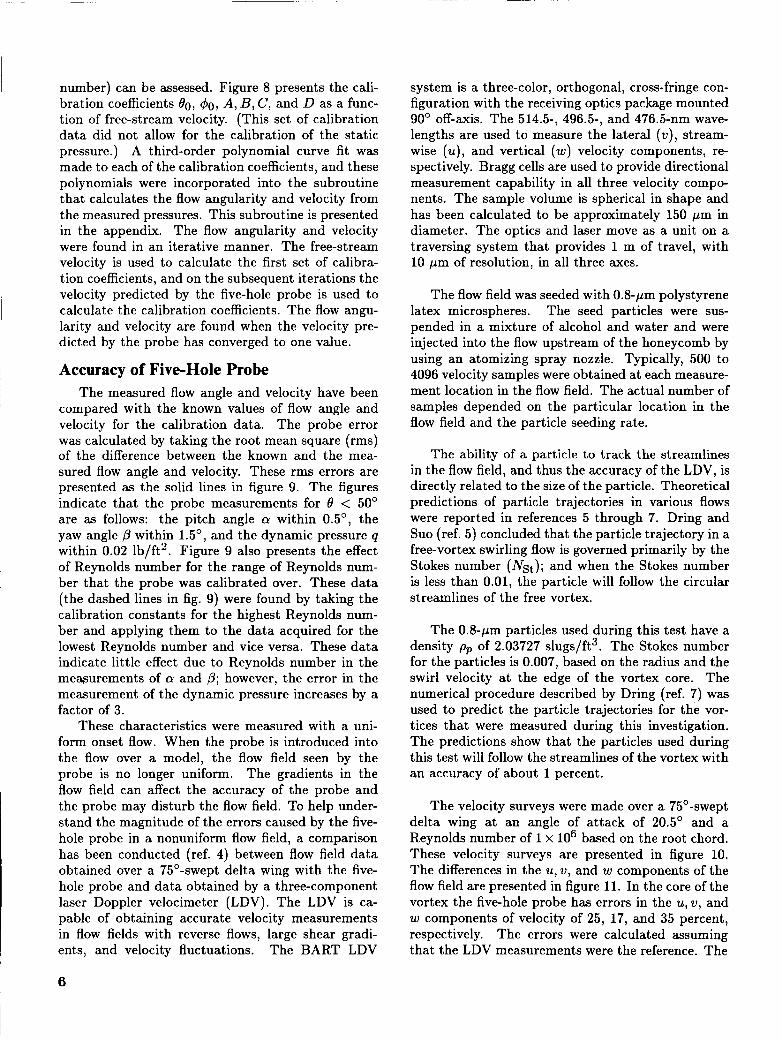
number) can be assessed. Figure 8 presents the cali- bration coefficients 80, 40, A , B, C, and D as a func- tion of free-stream velocity. (This set of calibration data did not allow for the calibration of the static pressure.) A third-order polynomial curve fit was made to each of the calibration coefficients, and these polynomials were incorporated into the subroutine that calculates the flow angularity and velocity from the measured pressures. This subroutine is presented in the appendix. The flow angularity and velocity were found in an iterative manner. The free-stream velocity is used to calculate the first set of calibra- tion coefficients, and on the subsequent iterations the velocity predicted by the five-hole probe is used to calculate the calibration coefficients. The flow angu- larity and velocity are found when the velocity pre- dicted by the probe has converged to one value.

Accuracy of Five-Hole Probe The measured flow angle and velocity have been

compared with the known values of flow angle and velocity for the calibration data. The probe error was calculated by taking the root mean square (rms) of the difference between the known and the mea- sured flow angle and velocity. These rms errors are presented as the solid lines in figure 9. The figures indicate that the probe measurements for 0 < 50' are as follows: the pitch angle a within 0.5', the yaw angle /3 within 1.5', and the dynamic pressure q within 0.02 lb/ft2. Figure 9 also presents the effect of Reynolds number for the range of Reynolds num- ber that the probe was calibrated over. These data (the dashed lines in fig. 9) were found by taking the calibration constants for the highest Reynolds num- ber and applying them to the data acquired for the lowest Reynolds number and vice versa. These data indicate little effect due to Reynolds number in the mewurements of a and /3; however, the error in the measurement of the dynamic pressure increases by a factor of 3.

These characteristics were measured with a uni- form onset flow. When the probe is introduced into the flow over a model, the flow field seen by the probe is no longer uniform. The gradients in the flow field can affect the accuracy of the probe and the probe may disturb the flow field. To help under- stand the magnitude of the errors caused by the five- hole probe in a nonuniform flow field, a comparison has been conducted (ref. 4) between flow field data obtained over a 75O-swept delta wing with the five- hole probe and data obtained by a three-component laser Doppler velocimeter (LDV). The LDV is ca- pable of obtaining accurate velocity measurements in flow fields with reverse flows, large shear gradi- ents, and velocity fluctuations. The BART LDV

6

system is a three-color, orthogonal, cross-fringe con- figuration with the receiving optics package mounted 90' off-axis. The 514.5-, 496.5-, and 476.5-nm wave- lengths are used to measure the lateral (v), stream- wise (u) , and vertical (w) velocity components, re- spectively. Bragg cells are used to provide directional measurement capability in all three velocity compo- nents. The sample volume is spherical in shape and has been calculated to be approximately 150 pm in diameter. The optics and laser move as a unit on a traversing system that provides 1 m of travel, with 10 pm of resolution, in all three axes.

The flow field was seeded with 0.8-pm polystyrene latex microspheres. The seed particles were sus- pended in a mixture of alcohol and water and were injected into the flow upstream of the honeycomb by using an atomizing spray nozzle. Typically, 500 to 4096 velocity samples were obtained at each measure- ment location in the flow field. The actual number of samples depended on the particular location in the flow field and the particle seeding rate.

The ability of a particle to track the streamlines in the flow field, and thus the accuracy of the LDV, is directly related to the size of the particle. Theoretical predictions of particle trajectories in various flows were reported in references 5 through 7. Dring and Suo (ref. 5) concluded that the particle trajectory in a free-vortex swirling flow is governed primarily by the Stokes number (Ns t ) ; and when the Stokes number is less than 0.01, the particle will follow the circular streamlines of the free vortex.

The 0.8-pm particles used during this test have a density p p of 2.03727 slugs/ft3. The Stokes number for the particles is 0.007, based on the radius and the swirl velocity at the edge of the vortex core. The numerical procedure described by Dring (ref. 7) was used to predict the particle trajectories for the vor- tices that were measured during this investigation. The predictions show that the particles used during this test will follow the streamlines of the vortex with an accuracy of about 1 percent.

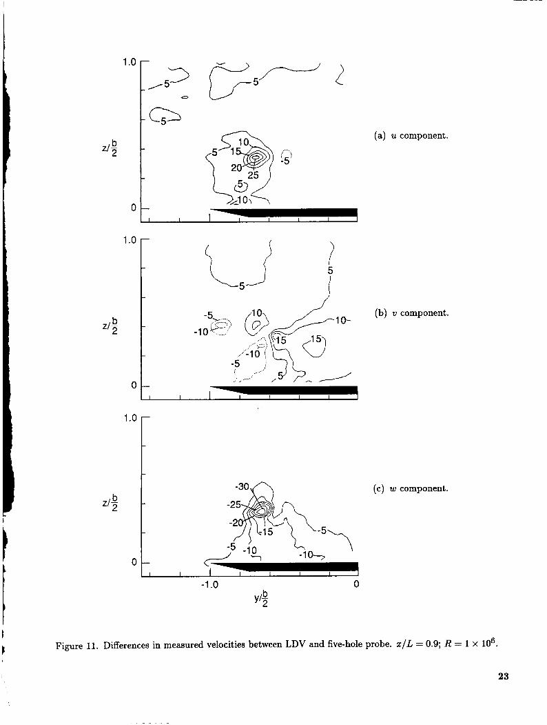
The velocity surveys were made over a 75O-swept delta wing at an angle of attack of 20.5' and a Reynolds number of 1 x lo6 based on the root chord. These velocity surveys are presented in figure 10. The differences in the u, v, and w components of the flow field are presented in figure 11. In the core of the vortex the five-hole probe has errors in the u, v, and w components of velocity of 25, 17, and 35 percent, respectively. The errors were calculated assuming that the LDV measurements were the reference. The

equation used to calculate the u-component error is

where the subscript FH denotes the five-hole probe. The errors in w and w are calculated in a similar fashion.

Figure 12 presents the gradients in the w and w components of velocity measured by the five-hole probe for the same data set. A comparison of fig- ures 11 and 12 shows that the probe does a reason- able job of measuring the flow field quantities in re- gions of low gradients (with a probe error less than 5 percent when the velocity gradient is less than 800&/ft). However, in the vortex core, very high gradients (> 3000&/ft) yield differences of more than 20 percent between the two measurement tech- niques.

Concluding Remarks A technique has been presented for the calibration

of a hemispherical-tipped, five-hole probe with a 0.125-in. diameter. Equations were derived from the potential flow over a sphere relating the flow angle and velocity to pressure differentials measured by the probe. Four sets of calibration data were acquired at eight free-stream velocities. A set of calibration data was obtained by yawing the probe between -90' and 90' in 1' increments. The four

data sets were obtained by rolling the probe through 90' increments. The calibration data are fit to the equations derived from the potential flow over a sphere to obtain the calibration coefficients, which are then used to convert measured pressures into flow angularity and velocity data.

To assess the ability of the five-hole probe to mea- sure flow angularity and velocity, the known calibra- tion data were compared with those measured by the five-hole probe. For the uniform flow field measured for the probe calibration, the probe measurements were as follows for a total angle of total-pressure port to stagnation point less than 50': the pitch an- gle within 0.5', the yaw angle within 1.5', and the dynamic pressure within 0.02 lb/ft2. For the non- uniform flow over a 75O-swept delta wing, com- parisons between the five-hole probe and a three- component laser Doppler velocimeter showed that the probe performed a reasonable job of measuring the flow field quantities in regions of low gradients (with a probe error less than 5 percent when the ve- locity gradient is less than 800&/ft). However, in the vortex core, very high gradients (> 3000&/ft) yielded differences of more than 20 percent between the two measurement techniques.

NASA Langley Research Center Hampton, VA 23665-5225 September 20, 1988

I

/"

,,,/

i Appendix

Listing of Five-Hole-Probe Subroutine i

This subroutine is used to convert the pressures measured by the yaw-pitch probe into flow velocity and angularity.

C C C C C C C C C C

I C C C C C C C C C C C

‘

SUBROUTINE FIVEHOLE(P,ALPHA,BETA,THETA,PHI,Q,PS,VELJ’REV)

FIVEHOLE CONVERTS MEASURED PRESSURES INTO FLOW ANGLES AND VELOCITY DATA USING THE CALIBRATION EQUATIONS DERIVED IN APPENDIX A OF REFERENCE 2

SUBROUTINE WRITTEN BY KJELGAARD IN AUGUST 1986 DESCRIPTION OF VARIABLES INPUT

P - ARRAY CONTAINING PRESSURES MEASURED BY 5-HOLE PROBE P(l) CONTAINS PRESSURE AT PORT 1 P(2) CONTAINS PRESSURE AT PORT 2, ETC.

OUTPUT ALPHA - PITCH ANGLE MEASURED BY PROBE BETA THETA - TOTAL FLOW ANGLE MEASURED FROM PORT 1 TO STAGNATION

- YAW ANGLE MEASURED BY PROBE

POINT - FLOW ROLL ANGLE MEASURED FROM LOWER ALPHA PORT TO STAGNATION POINT

PHI

Q PS VEL-PREV - VELOCITY USED TO CALCULATE PROBE CONSTANTS

- DYNAMIC PRESSURE OF THE FLOW AT THE PROBE TIP - STATIC PRESSURE MEASURED AT THE PROBE TIP

c- C

REAL P(*) REAL ALPH(2) ,BET(2) ,THET(B) ,QT(2) ,PST(2) REAL A(2) ,THETAO( 2) ,PHIO( 2) ,B( 2) ,C( 2) ,D( 2) ,E( 2) ,F (2) ,G(2) EXTERNAL POLY DPA=P (6)-P (5) DPB=P(3)-P(4) QP=P( 1)-.25* (P( 3)+P(4) +P( 5)+P(6)) Al=SQRT(DPA**2+DPB**2)/QP

PROBE CONSTANTS

A( l)=POLY (VELPREV,.l3930,-2.5727E-3,1.43414E-5,0) A(2)=POLY (VELPREV,3.1607,-8.1927E-3,7.175OE-5,-1.8642E7) THETAO( l)=POLY (VELPREV,55.595,-5.862lE2,4.7727E4,- 1.14273-6) THETAO( 2)=POLY (VEL-PREV,57.134,-9.3249E-2,8.0274E-4,-2.0331E6) B ( l)=POLY (VELPREV, .31547,2.4019E2 ,-2.0699E4,5.5 1563-7) B( 2)=POLY (VELPREV , .67481,9.7006E-3,-7.1074E5,1.4787E-7) PHIO( 1)zPOLY (VELJ’REV,-.48446,-4.9767E2,4.5553E-4,-1.2265E-6) PHIO(S)=POLY (VELPREV,-4.2108,4.5463E-2,-2.7104E-4,4.4549E-7) C( 1)EPOLY (VELPREV,.25419,-1.674lE-3,9.327OE6,-8.6405E9) C(2)=POLY (VELPREV,.38568,-5.2703E-3,3.7782E5,-8.2944E-8) D( l)=POLY (VELJ’REV,.74529,1.7064E-2,-1.1424E4,2.2726E7) D(2)zPOLY (VELPREV,.23948,2.9862E2,-2.1885E4,5.0793E-7)

C C ITERATIVELY SOLVE FOR THETA

DO 1 I=1,2 THET(I)=O. THSTEP=10.

CALCULATE PHI

IF (DPA .EQ. 0) DPA=.00001 PHIM=ATAND(B(I) *DPB/DPA) IF (DPA .LT. 0) PHIM=180.+PHIM IF (PHIM .LT. 0) PHIM=PHIM+360. PHIT=PHIM-PHIO( I) A2=1 DO 2000 ILOOP=1,50

IF (ILOOP .EQ.50) THEN WR"E(G,'('' TOO MANY ITERATIONS IN CALB")') THET(I)=.5*ACOSD(A(I)*SIND(2.*THETAO(I))/Al+

GO TO 3170 * COSD(2.*THETAO(I)))

END IF THET(I)=THET(I) + THSTEP A3=COSD(2.*THET(I))-COSD(2.*THETAO(I)) IF (A3.EQ.0.0) THEN

WR"E(G,'('' PROBLEM IN CALIB")') WRITE( 6, ' (4F 10.5) ') THET( I) ,THSTEP A3=1E-5

END IF

IF (A2 .LT. 0) THEN AP=Al-A(I)*SIND(2.*THET(I))/AS

THET( I) =THET (1)-THSTEP THSTEP=THSTEP*.5 GO T O 3160

END IF IF (A2 .LE. .02) GO T O 3170

3160 CONTINUE 2000 CONTINUE 3170 ALPH(1) =ATAND( TAND (THET(1)) *COSD( PHIT))

BET(I)=ASIND( SIND( THET(I)) *sIND (PHIT)) QT(I)~QP/(C(I)*(COSD(2.*THET(I))-COSD(2.*THETAO(I)))+

PST(I)~P(1)-QT(I)*(E(I)*COSD(2.*THET(I))+F(I)*COSD(THET(I)) * D(I)*(COSD(THET(I))-COSD(THETAO(1))))

* +G(I)) 1 CONTINUE C C C C

USE PHI FOR WEIGHTING FUNCTION FOR COMBINATION OF ALPHA AND BETA CONSTANTS AND COMBINE

WGHT=COSD(PHI) **2

BETA=BET( 1)* WGHT+BET(2)* WGHTl ALPHA=ALPH( l)*WGHT+ALPH(2)*WGHTl Q=QT( 1) * WGHT+QT(2) * WGHTl PS=PST( 1)* WGHT+PST(2)* WGHTl

USE THESE TO CALCULATE THETA AND PHI

WGHT1=1- WGHT

C C

9

C THETA=ACOSD(COSD(ALPHA)*COSD(BETA)) IF (ALPHA .EQ. 0) THEN

PHI=SIGN(SO.,BETA) ELSE

PHI=ATAND (TAND (BETA) /SIND (ALPHA)) END IF IF (ALPHA .LT. 0) PHI= PHI+180. IF (PHI .LT. 0) PHI= PHI+360.

!

RETURN END

FUNCTION POLY (V,A,B,C,D) POLY = A + B*V + C*V*V + D*V*V*V RETURN END

10 I

I

References 1. Bryer, D. W.; and Pankhurst, R. C.: Pressure-Probe

Methods for Determining Wind Speed and Flow Direction. Her Majesty’s Stationery Off. (London), 1971.

2 . Fearn, Richard L.; and Weston, Robert P.: Induced Velocity Field of a Jet in a Crossflow. NASA TP-1087, 1978. Nielsen, Kaj L.: Methods in Numerical Analysis, Second ed. Macmillan Co., 1964. Kjelgaard, Scott 0.; and Sellers, William L., 111: De- tailed Flowfield Measurements Over a 75’ Swept Delta

3.

4.

Wing for Code Validation. Paper presented at the AGARD Symposium on Validation of Computational Fluid Dynamics (Lisbon, Portugal), May 2-5, 1988.

5. Dring, R. P.; and Suo, M.: Particle Trajectories in Swirling Flows. J. Energy, vol. 2, July-Aug. 1978,

6. Dring, R. P.; Caspar, J. R.; and Suo, M.: Particle Trajectories in Z’urbine Cascades. J. Energy, vol. 3, no. 3, May-June 1979, pp. 161-166.

7. Dring, R. P.: Sizing Criteria for Laser Anemometry Particles. lkans. ASME, J . Fluids Eng., vol. 104, Mar.

pp. 232-237.

1982, pp. 15-17.

I

11

a

L

a

L

l a

h

a a a 3 5

I

a,

Lo cu

ru 0

I 12

7fx

I

5

/

Probe axes systems

Figure 2. Coordinate system of five-hole probe.

-3 20 -80 -40 0 40 80 120

V! deg

Figure 3. Typical set of calibration data.

13

(a) Section illustrating probe misalignment with free stream. View looking down from above.

(b) Plot illustrating probe misalignment in yaw with free stream.

Figure 4. Yaw error due to misalignment with free stream.

14

Roll of 0" UCO

UCO Roll of 180"

(a) Sketch illustrating manufacturing error. View looking down from above.

.6

.4

.2

APp 'q 0

-.2

-.4

-.6

(b) Plot illustrating probe manufacturing error in ,B ports.

Figure 5. Manufacturing error in p ports.

15

Ua,

Roll of 0"

u w

Roll of 180"

Figure 6 . Sketch illustrating probe error in pitch due to misalignment with free stream. View looking from side.

.2

-.2

-.4 0 4

Figure 7. Typical data set presenting uncorrected calibration data.

16

0 -0

c\1

0 -a T-

o o -a Q,

- 3 .c

8 3

-0 03

0

6ap ' O d

6ap 'On

0 0 N

3 a r

3 0 N Q , v 3 .c

8 3

3 33

3 d

0 0 cu

0 (D 7

0 0 c u m - v )

5

8 2,

.c

0 co

0

17

0

a 2 0

ru 0

0

0 0 (u

0 co T

o v ( u a , - 3 -

8 3

0 a3

0

n rw V

n 4 V I

V

I I I I 0 03 0 d

c9 o! @i cu c9

V cu c9 cu cu

I I 6ap lo@

18

i

0 -0

N

0 -a Y

0 0 - N a, - 0 c

8 3

-0 co

0

0

0 0 a0 d

a 1 0 0 c 0 m d d

2 CE]

8 b

&l

0 -0

N

0 -a 7

0 0 - N a, - c n

2 8

3

-0 co

0 0 b e4 a !3

0 0 0, c 0 m d d

2 CEl 8 b

$4

0

0 0

a 2 8 0 0 +I 0 m d d

2 CE]

8 b

&l

0 0 P- m

1 Ld 0 0 Q,

0 c

m d d

2 CEl Ll

19

0

0 0 N

0 (D 7

0 0 N U

r 3 c

8 3

3 P

3 e I I I I I I

( 4 L o L n Y Y T O ( D N c o d . 0

20

2.0r I I

1

I I

2.4 - 2.0 -

I

(b) rms error in keas versus 8.

1.6 -

1.2 -

0 I I

a 3 r I

(c) rms error in qmeas versus e.

-

Cali brat ion constants

Correct _ _ _ - Incorrect

Figure 9. Characteristics of probe calibrated in this investigation.

21

Y b

I

1 I

I

I

.5 c I

I

- ua2 I

-1 .o -.5 0

(a) Crossflow velocity vectors measured with five-hole probe.

-1 .o -.5 0

I (b) Crossflow velocity vectors measured with three-component laser Doppler velocimeter.

Figure 10. Velocity surveys obtained over 75O-swept delta wing at an angle of attack of 20.5’, x / L = 0.9, and R = 1 x lo6.

I 22

I

1 .o

21, b

0

b5' (a) u component.

1 .o

21, b

n

- 3 0 0 b -

-

21,

0 - I I I

-1 .o 0 b YJZ

(b) TI component.

(c) w component.

Figure 11. Differences in measured velocities between LDV and five-hole probe. x / L = 0.9; R = 1 x lo6.

23

1 .o

21, b

0

0

\

I I I I I I I I I -1 .o 0

(a) Gradient of lateral component of velocity nondimensionalized by maximum of 6111 &/ft.

1 .o

21, b

0

d

-1 .o 0

(b) Gradient of vertical component of velocity nondimensionalized by maximum of 7074 &/ft.

Figure 12. Velocity gradients calculated from five-hole-probe results.

24

Report Documentation Page

1. Report No. 2. Government Accession No. NASA TM-4047

1. Title and Subtitle

3. Recipient's Catalog No.

5. Report Date

6. Performing Organization Code

Theoretical Derivation and Calibration Technique of a Hemispherical-Tipped, Five-Hole Probe

3. Performing Organization Name and Address NASA Langley Research Center Hampton, VA 23665-5225

8. Performing Organization Report No. 7. Author(s)

L-16454 Scott 0. Kjelgaard

10. Work Unit No.

505-60-1 1-03 11. Contract or Grant No.

12. Sponsoring Agency Name and Address National Aeronautics and Space Administration Washington, DC 20546-0001

13. Type of Report and Period Covered

Technical Memorandum 14. Sponsoring Agency Code

16. Abstract A technique is presented for the calibration of a hemispherical-tipped, five-hole probe having a 0.125- in. diameter. Equations are derived from the potential flow over a sphere relating the flow angle and velocity to pressure differentials measured by the probe. The technique for acquiring the calibration data and the technique for calculating the calibration coefficients are presented. The accuracy of the probe in both the uniform calibration flow field and the nonuniform flow field over a 75O-swept delta wing is discussed.

his page)

17. Key Words (Suggested by Authors(s)) Pressure probe Yaw-pitch probe Five-hole probe Probe calibration

19. Security Classif.(of this report) 120. Security Classif.(of 21. No. of Pages 22. Price 25 A02

18. Distribution Statement Unclassified-Unlimited

lASA FORM 1626 OCT 86 NASA-Langley, 1988

For sale by the National Technical Information Service, Springfield, Virginia 22161-2171