Theoretical and Phenomenological Study of G2Compactifications of M Theory

by

Ran Lu

A dissertation submitted in partial fulfillmentof the requirements for the degree of

Doctor of Philosophy(Physics)

in the University of Michigan2013

Doctoral Committee:

Professor Gordon L. Kane, ChairProfessor Lizhen JiProfessor Finn LarsenAssociate Professor Aaron T. PierceProfessor Bing Zhou

©Ran Lu

2013

A C K N O W L E D G M E N T S

This thesis would have been impossible without the excellent support of myadvisor, Gordon Kane. I am very lucky to have the opportunity to work withyou and I sincerely grateful for all that you have done for me.I would also like to thank my collaborators: Bobby Acharya, Daniel Feldman,Eric Kuflik, Piyush Kumar, Brent Nelson, LianTao Wang, Scott Watson andBob Zheng. It has been a great pleasure to work with all of you and I learnedso much during our collaborations.I have had helpful discussions with many other people, including (non-exhaustively): Michele Cicoli, Jim Halverson, Jack Kearney, Ian-Woo Kim,Finn Larsen, Jim Liu, Sam McDermott, Malcolm Perry, Aaron Pierce, StuartRaby, Saul Ramos-Sanchez, and Haibo Yu.

ii

TABLE OF CONTENTS

Acknowledgments . . . . . . . . . . . . . . . . . . . . . . . . . . . . . . . . . . . . . . . ii

List of Figures . . . . . . . . . . . . . . . . . . . . . . . . . . . . . . . . . . . . . . . . . v

List of Tables . . . . . . . . . . . . . . . . . . . . . . . . . . . . . . . . . . . . . . . . . . viii

Abstract . . . . . . . . . . . . . . . . . . . . . . . . . . . . . . . . . . . . . . . . . . . . . x

Chapter

1 Introduction . . . . . . . . . . . . . . . . . . . . . . . . . . . . . . . . . . . . . . . . . 1

1.1 Introduction . . . . . . . . . . . . . . . . . . . . . . . . . . . . . . . . . . . . . 1

2 M theory compactification on G2 manifolds . . . . . . . . . . . . . . . . . . . . . . . . 4

2.1 G2 manifolds . . . . . . . . . . . . . . . . . . . . . . . . . . . . . . . . . . . . 42.2 Matter and Gauge Theory . . . . . . . . . . . . . . . . . . . . . . . . . . . . . . 42.3 Moduli Stabilization . . . . . . . . . . . . . . . . . . . . . . . . . . . . . . . . 52.4 Geometric Symmetries and Moduli Transformations . . . . . . . . . . . . . . . . 92.5 Discrete symmetries and Moduli Stabilization . . . . . . . . . . . . . . . . . . . 10

3 G2-MSSM . . . . . . . . . . . . . . . . . . . . . . . . . . . . . . . . . . . . . . . . . . 12

3.1 The spectrum . . . . . . . . . . . . . . . . . . . . . . . . . . . . . . . . . . . . 123.2 Doublet-triplet splitting and µ . . . . . . . . . . . . . . . . . . . . . . . . . . . 14

3.2.1 Review of Witten’s Proposal . . . . . . . . . . . . . . . . . . . . . . . . 153.2.2 An Aside: R versus Non-R Discrete Symmetry . . . . . . . . . . . . . . 173.2.3 Generating µ via Moduli Stabilization . . . . . . . . . . . . . . . . . . . 173.2.4 Non-Perturbative Contributions to µ . . . . . . . . . . . . . . . . . . . . 203.2.5 Constraints on the (approximate) ZN Symmetry . . . . . . . . . . . . . 223.2.6 The Necessity of Another Exact Symmetry . . . . . . . . . . . . . . . . 253.2.7 Embedding ZM within ZN . . . . . . . . . . . . . . . . . . . . . . . . . 26

3.3 Electroweak Symmetry Breaking and Little Hierarchy Problem . . . . . . . . . . 283.3.1 Electroweak Symmetry Breaking . . . . . . . . . . . . . . . . . . . . . 293.3.2 Renormalization Group Equations of MSSM . . . . . . . . . . . . . . . 303.3.3 General Mechanism and Numerical Results . . . . . . . . . . . . . . . . 32

4 Cosmology and Dark Matter . . . . . . . . . . . . . . . . . . . . . . . . . . . . . . . . 38

4.1 Cosmological Moduli/Gravitino Problem . . . . . . . . . . . . . . . . . . . . . . 384.2 Dark Matter Candidates in G2-MSSM . . . . . . . . . . . . . . . . . . . . . . . 39

iii

4.3 The non-thermal WIMP ‘Miracle’ . . . . . . . . . . . . . . . . . . . . . . . . . 404.4 Indirect Detection . . . . . . . . . . . . . . . . . . . . . . . . . . . . . . . . . . 40

4.4.1 GALPROP Parameters . . . . . . . . . . . . . . . . . . . . . . . . . . . 454.4.2 Solar Modulation . . . . . . . . . . . . . . . . . . . . . . . . . . . . . . 474.4.3 Astrophysical Flux . . . . . . . . . . . . . . . . . . . . . . . . . . . . . 524.4.4 Density Fluctuation Factor . . . . . . . . . . . . . . . . . . . . . . . . . 52

4.5 Direct Detection . . . . . . . . . . . . . . . . . . . . . . . . . . . . . . . . . . . 54

5 The Mass of the Lightest Higgs Particle . . . . . . . . . . . . . . . . . . . . . . . . . . 56

5.1 Higgs Mass Calculation . . . . . . . . . . . . . . . . . . . . . . . . . . . . . . . 565.2 The Higgs and BSM Physics . . . . . . . . . . . . . . . . . . . . . . . . . . . . 585.3 Computation of the Higgs Mass . . . . . . . . . . . . . . . . . . . . . . . . . . 60

5.3.1 Matching at Msusy . . . . . . . . . . . . . . . . . . . . . . . . . . . . . 615.3.2 Two -loop RGEs and Weak Scale Matching . . . . . . . . . . . . . . . . 61

5.4 Result . . . . . . . . . . . . . . . . . . . . . . . . . . . . . . . . . . . . . . . . 62

6 Gluino and Chargino Searches at the LHC . . . . . . . . . . . . . . . . . . . . . . . . 65

6.1 General Gluino Search Signatures . . . . . . . . . . . . . . . . . . . . . . . . . 656.2 Discovery Prospects and Concrete Signatures . . . . . . . . . . . . . . . . . . . 66

6.2.1 Global Analysis and Discovery Prospects of SUSY . . . . . . . . . . . 686.3 Third family enhanced gluino decays . . . . . . . . . . . . . . . . . . . . . . . . 70

6.3.1 Benchmark Models . . . . . . . . . . . . . . . . . . . . . . . . . . . . . 716.3.2 Signal Isolation and Backgrounds . . . . . . . . . . . . . . . . . . . . . 71

6.4 Searching for Gluino Events with W± Tracks . . . . . . . . . . . . . . . . . . . 736.5 Reconstructing the Gluino Mass . . . . . . . . . . . . . . . . . . . . . . . . . . 78

7 Conclusion . . . . . . . . . . . . . . . . . . . . . . . . . . . . . . . . . . . . . . . . . . 80

7.1 conclusion and future directions . . . . . . . . . . . . . . . . . . . . . . . . . . 80A.1 Implications of Top-Down Constraints . . . . . . . . . . . . . . . . . . . . . . . 82

A.1.1 Constraints on Wilson Line Parameters from Anomaly Cancellation . . . 82A.1.2 Fermion Mass Forbidden by ZN . . . . . . . . . . . . . . . . . . . . . . 83A.1.3 Constraints on the LSP Lifetime . . . . . . . . . . . . . . . . . . . . . . 84

A.2 Largest Spin Independent Cross Sections . . . . . . . . . . . . . . . . . . . . . . 85

Appendix . . . . . . . . . . . . . . . . . . . . . . . . . . . . . . . . . . . . . . . . . . . . 82

Bibliography . . . . . . . . . . . . . . . . . . . . . . . . . . . . . . . . . . . . . . . . . . 88

iv

LIST OF FIGURES

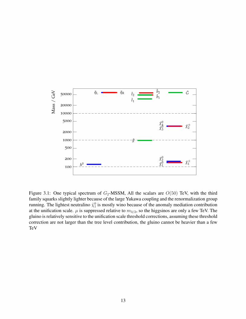
3.1 One typical spectrum of G2-MSSM, All the scalars are O(50) TeV, with the thirdfamily squarks slightly lighter because of the large Yukawa coupling and the renor-malization group running. The lightest neutralino χ0

1 is mostly wino because of theanomaly mediation contribution at the unification scale. µ is suppressed relative tom3/2, so the higgsinos are only a few TeV. The gluino is relatively sensitive to the uni-fication scale threshold corrections, assuming these threshold correction are not largerthan the tree level contribution, the gluino cannot be heavier than a few TeV . . . . . . 13

3.2 The 1 loop RGE coefficients fM0 and fA0 atQEWSB as given in Eq.(3.65). The amountof cancellation in the Eq.(3.65) for m2

Hu(QEWSB) depends on |A0|/M0, and we show

the values that minimize m2Hu

at one-loop. In this figure, M0 runs from 10 TeV at thelower end of the curve to 50 TeV at the top of the curve. (See Fig. (3.4) for the fullanalysis with with 2 loop running and the threshold/radiative corrections.) . . . . . . 33

3.3 Two-loop renormalization group running of mHu for 3 models for the cases M0 =(10, 30, 50) TeV. The tadpole corrections are shown, and appear as a vertical drop atQEWSB =

√mt1

mt2as is appropriate. The numerical value of mHu , which is the tree

+ tadpole value, continue to take the same value at scales Q below the point QEWSB

as is theoretically expected. The values of µ are µ = (500 GeV, 1.0 TeV, 1.8 TeV).This can be seen for example for the M0 = 30 TeV in figure 3.4 using Eq. (3.43). . . 34

3.4 A large parameter space sweep using the full numerical analysis discussed in the textforM0 = 30 TeV, with µ ∈ [0.9, 2] TeV, with tan β ∈ [3, 15] showing a robust regionwhere mHu , the loop corrected value at the EWSB scale, is reduced significantly rel-ative to M0 = 30 TeV, with the greatest suppression occurring for trilinear of aboutthe same magnitude. . . . . . . . . . . . . . . . . . . . . . . . . . . . . . . . . . . . 35

4.1 The positron flux ratio, generated with the parameters described in the text and Table4.1 with a MW = 180 GeV wino. The solid line is the ratio of the total positron flux,which includes the positrons from the wino annihilation, the astrophysical flux andthe conventional astrophysics background to positrons plus electrons. The long dashline contains just the wino annihilation and the conventional astrophysics background,and the short dash line is the ratio of the secondary positrons only.The data are from[1] and [2], Our analysis assumes the reported normalization of the PAMELA andAMS-02 data. If those change it will affect the higher energy extrapolation here. . . . 48

v

4.2 The antiproton flux ratio. The solid line is the ratio of the total antiproton flux, whichinclude the antiproton from wino annihilation, and conventional astrophysics back-ground, the dash line has the same components but without the density fluctuationfactor, the dot line is astrophysics background only. The data are from PAMELA [3].Note the signal is larger than the background down to very low energies. . . . . . . . . 49

4.3 The Boron to Carbon ratio with our standard parameters, solar modulation effect isnot included, The data are from [4]. . . . . . . . . . . . . . . . . . . . . . . . . . . . 50

4.3 The Boron to Carbon ratio with one parameter different (δ changes from 0.5 to 0.4).This illustrates that the Boron to Carbon ratio is very sensitive the diffusion parame-ters. The data are from [4]. . . . . . . . . . . . . . . . . . . . . . . . . . . . . . . . . 51

4.4 The absolute flux of e++e−, The solid line is the sum of electron and positron from thewino annihilation, the density fluctuation factor, our assumed extra flux, and conven-tional astrophysics background, the dash line has the same components but withoutthe density fluctuation factor. The dash-dot line contains wino annihilation and as-trophysics background, and the dot line is the conventional astrophysics backgroundonly. See comments in Figure 4.1. The data are from [5]. . . . . . . . . . . . . . . . . 53

5.1 The prediction for the Higgs mass at two-loops for realistic string/M theory vacua definedin the text, as a function of tanβ for three different values of the gravitino mass m3/2, andvarying the theoretical and experimental inputs as described below. For precise numbers andmore details, see section 5.4. The central band within the dashed curves for which scatterpoints are plotted corresponds to m3/2 = 50 TeV. This band includes the total uncertainty inthe Higgs mass arising from the variation of three theoretical inputs at the unification scale,and from those in the top mass mt and the SU(3) gauge coupling αs within the alloweduncertainties. The innermost (white) band bounded by solid curves includes the uncertainty inthe Higgs mass for m3/2 = 50 TeV only from theoretical inputs. The upper (dark gray) bandbounded by solid curves corresponds to the total uncertainty in the Higgs mass for m3/2 =

100 TeV while the lower (light gray) band bounded by solid curves corresponds to that form3/2 = 25 TeV. For m3/2 = 50 TeV, the red scatter points (with tanβ less than about4.5) and blue scatter points (with tanβ greater than about 4.5) correspond to “Large” µ and“Small” µ respectively, as described in section 5.2 and section 5.4. . . . . . . . . . . . . . . 57

6.1 Upper left panel: M4jetseff =

∑J=1−4 P

JT (J) + Pmiss

T at 10 TeV with 1 fb−1 for the G12

model benchmark with ST ≥ 0.25 (transverse sphericity), PmissT ≥ 200 GeV and a

lepton veto. The backgrounds mainly comes from dijets, tt and W+ jets. Upper rightpanel: Distribution of jet number showing excesses in events with large jet multiplic-ities at low luminosity. Lower left panel: Discovery reach for the same model with√s = (7, 10, 14) TeV. Lower right panel: Same model and cuts as the upper panel

for 14 TeV with 5 fb−1 in the variable M2beff =

∑J=1−2 P

bT (J) + Pmiss

T . . . . . . . . . 676.2 Ratio of gaugino masses in the G2 model. The predicted ratios can be quite different

than those that arise in other models of soft SUSY breaking (for a comparison see Ref.[6]). The mass range here for the wino is (170 - 210) GeV and the gluino lies in therange (500-900) GeV. . . . . . . . . . . . . . . . . . . . . . . . . . . . . . . . . . . 70

vi

6.3 Charged Winos resulting from gluino pair production, binned as a function of trans-verse distance traveled from the beam line. These results correspond to 10 fb−1 ofLHC-8 data (σgg ∼ 235 fb), with mg = 750 GeV, mW = 150 GeV. For graphicalpurposes, charginos traveling a transverse distance < 30 cm are not shown. . . . . . . 76

vii

LIST OF TABLES

3.1 Non anomalous Z4 symmetry which satisfies Wilson line and phenomenological con-straints. This symmetry is manifestly anomaly free and does not require any GSmechanism for anomaly cancellation. One of the down quark masses is forbiddenby this Z4, and therefore must be radiatively generated once the symmetry is broken,for example by non-holomorphic Higgs coupling between the Hu and the down-typequarks/leptons. If all moduli fields have even charge under this Z4, this Z4 symmetrycan be broken to an exact Z2 R-parity upon moduli stabilization. . . . . . . . . . . . . 28

4.1 The parameters used for simulation. The physical meaning of these parameters isdescribed in the text. . . . . . . . . . . . . . . . . . . . . . . . . . . . . . . . . . . . 46

5.1 Uncertainties in the calculation of the Higgs mass for a given value ofm3/2 and tan β,as shown in Figure 1. All masses are in GeV. . . . . . . . . . . . . . . . . . . . . . . 63

5.2 Variation of the theoretical and experimental inputs. All masses are in GeV. . . . . . . 63

6.1 Some benchmark models predicting a light gluino and a LSP that is a wino with adegenerate chargino with a light second neutralino (which is mostly bino). The lastfour columns carry units of GeV. . . . . . . . . . . . . . . . . . . . . . . . . . . . . 68

6.2 Dominant branching ratios of the gluinos. . . . . . . . . . . . . . . . . . . . . . . . 696.3 Shown is σSUSY(fb), the theoretical cross section before passing through the detector

simulation, σeff(fb), the effective cross section after events have passed the L1 triggerswith L = 1fb−1 at

√s = 10 TeV. Observable counts in the number of tagged b-

jets and multijets are also shown N(2b), N(4j) along with their signal to square rootbackground ratios. The missing energy cut is ≥ 200 GeV and we have imposed atransverse sphericity cut of ST ≥ 0.25. . . . . . . . . . . . . . . . . . . . . . . . . . 69

6.4 Relevant branching ratios for the benchmark models considered in this paper. Themodels A and B have bino LSP. In Model C, the lightest neutralino and lightestchargino are both winos. In all models the first two generation squark masses aretaken to be 8 TeV. The third generation is taken to be somewhat lighter and is chosento generate the required branching ratios of the model. . . . . . . . . . . . . . . . . . 71

viii

6.5 Cross sections for production of signal and backgrounds. The first column gives thetotal production cross section. The second gives the cross section after the L1 trig-gers defined in PGS-4 (see text). The remaining columns give the cross section afterselection cuts in Eq. 6.1 and Eq. 6.2, with an additional missing energy (MET) re-quirement, 6ET ≥ 100 GeV. The bb + jets and bbbb-inclusive backgrounds have beenconsidered, and after the applying the selection cuts in Eqs. 6.1-6.2 and requiring atleast one lepton, the number of events are negligible in the {b, `} channels consideredhere. In this table, we set mg = 500 GeV and mLSP = 100 GeV. . . . . . . . . . . . . 72

6.6 Number of SM events, number of signal event, and signal significance, with 2, 3, or4 b-tagged jets and OS, SS, or 3 leptons at the early LHC-7, for 1fb−1 integratedluminosity. For the 1-lepton counts, cut-1 was applied, while for the other leptoncounts cut-2 was applied. These numbers were found formg = 500 GeV andmLSP =100 GeV. . . . . . . . . . . . . . . . . . . . . . . . . . . . . . . . . . . . . . . . . . 74

6.7 Inclusive count of the number of charginos which make it past a given detector layer.These results correspond to 10 fb−1 of LHC-8 data (σgg ∼ 235 fb), with mg = 750 GeV. 75

6.8 Number of charginos which make it past the 3rd SCT layer in signal regions of variousATLAS SUSY search channels. These results are for 10 fb−1 of LHC-8 data. Wehave chosen channels expected to be sensitive to gluino pair production events. Othersearch channels give weaker chargino signals, which can be enhanced by looseningcuts. The meff cuts are given in units of GeV. . . . . . . . . . . . . . . . . . . . . . . 77

ix

ABSTRACT

Theoretical and Phenomenological Study of G2 Compactifications of M Theory

by

Ran Lu

Chair: Gordon Kane

This thesis focuses on the study of G2 compactification of M theory. With the as-

sumption that the low energy effective theory is the minimal supersymmetric standard

model (MSSM), these kinds of compactifications produce an interesting model called

G2-MSSM with distinctive particle spectrum. An approximate discrete symmetry on the

G2 manifold combined with symmetry breaking Wilson lines provide a solution to the

doublet-triplet splitting problem and generate a suppressed µ term. This small µ term

is consistent with electroweak symmetry breaking and the so called “little hierarchy”

problem is alleviated in G2-MSSM. The phenomenology of G2-MSSM is also studied.

The lightest supersymmetric particle (LSP), which is almost always a wino, is stable be-

cause of the R-parity of the theory, and has the right relic abundance when non-thermally

produced by the moduli decay. And due to its large annihilation cross section, it might

provide a partial explanation of the signals observed by indirect detection experiments.

Because of the suppressed µ term, the mass of the lightest Higgs particle in G2-MSSM

is about 125 GeV when the scalars are O(50 TeV). The gauginos are much lighter than

the scalars in G2-MSSM. The gluino and chargino have interesting collider signals at the

LHC.

x

CHAPTER 1

Introduction

1.1 Introduction

String/M theory is a framework that may help to formulate a underlying theory to understand theworld better, If so, it will be essential to “compactify” the 10 dimensional string theories or the11 dimensional M theory to four dimensions. We concentrate on the best motivated case wherethe small dimensions are Planck scale size (but still large enough so the supergravity calculationsare reliable). Even though the energy scale of the extra dimensions is assumed to be much abovethe center-of-mass energy of collisions at the Large Hadron Collider (LHC), the extra dimensionsstill manifest themselves at lower energies through the presence of moduli fields. These are modesof the extra dimensional graviton whose vacuum-expectation-values (vev’s) determine the shapesand sizes that the extra dimensions take. Being modes of the extra dimensional graviton, themoduli couple to matter with Planck suppressed interactions universally. The moduli have to bestabilized since all couplings and masses are determined from their vev’s. Although understandingphenomenologically relevant supersymmetry breaking in string theory is a challenging task, manyresults, including those needed to calculate the Higgs boson mass, can be obtained with rathermild, well motivated assumptions.

G2 compactification of M theory (i.e. compactification on a manifold with G2 honolomy) hasmade a lot progress in the recent years. Due to the mathematical difficulties associated with con-structing G2 manifolds, studying string compactifications on Calabi-Yau manifolds was and still ismore popular than studying G2 compactifications. Calabi-Yau 3-folds and 4-folds are understoodmuch better than G2 manifolds, mainly because algebraic geometry is very powerful on complexmanifolds. Using Yau’s theorem[7] one only need to calculate the first chern class to check theexistence of Calabi-Yau structure. On the other hand, the only way to verify a manifold admitsa G2 structure is to show that there is actually a G2 invariant metric. However, moduli stabiliza-tion, which requires great effort in Calabi-Yau compactification, is simplified in the G2 case. Ona Calabi-Yau manifold, one needs to stabilize complex structure moduli and Kahler moduli sep-

1

arately, usually with different mechanisms. Because G2 manifolds only have geometric moduli,all of them can be stabilized using QCD like interactions. When there are gaugino condensationsas well as meson fields from quark condensations, it is possible to stabilize moduli to a de Sittervacuum with small cosmological constant. In the scenario studied in [8, 9], the F-terms of themoduli are much smaller than the F-term of the meson field.

In the simplest case, the low energy spectrum only contains the MSSM, and the effective theoryis called G2-MSSM. But due to the unification of the gauge couplings, one naturally expects thefield theory after compactification is a grand unification theory (GUT) like SU(5). Doublet-tripletsplitting must be implemented to maintain the gauge coupling unification. This is also related tothe so-called “µ problem” which is one of the most fundamental issues in making a systematictheory of the physical world. It is a large hierarchy problem, with µ naturally being of the orderthe unification scale, but only make sense if it were at the TeV scale. It will be shown in thefollowing chapters that there is an elegant solution using an approximate discrete symmetry on theG2 manifold, first studied by Witten. We extended the idea to embed µ in the theory with stabilizedmoduli and estimate its size, thus proposing a solution to this fundamental problem.

This also provides a new approach to the little hierarchy problem. Even though there are stillunsolved problems in G2 compactifications, it is possible to study the phenomenology with somemild assumptions about the spectrum. In this thesis I will mainly consider the G2-MSSM. Oncethe spectrum is fixed, it is straightforward to calculate the mass of the lightest Higgs particle, studynew physics signals at the LHC, and explore the implications for cosmology and dark matter.

The Standard Model suffers from “naturalness” or “hierarchy” problem(s). In addition to thewell-known technical naturalness problem of the Higgs, there is the basic question of the originof the electroweak scale. In the context considered here: the embedding of the (supersymmetric)Standard Model in a UV complete microscopic theory like string/M theory has to explain why theelectroweak scale is so much smaller than the natural scale in string theory, the string scale, whichis usually assumed to be many of orders of magnitude above the TeV scale. The µ parameter(which sets the masses of Higgsinos and contributes to the masses of Higgs bosons) must alsobe around TeV scale. The models we describe here, with softly broken supersymmetry, includesolutions for all of these problems.

The organization of this thesis is the following. In Chapter 2 we briefly review the theoreticalsetup of M theory compactified on G2-manifolds. Following this, in Chapter 3 we study the lowenergy effective theory G2-MSSM. We show the discrete symmetry provides a satisfying solutionto the doublet-triplet splitting problem. The discrete symmetry must be anomaly free, which putsnon-trivial constraints on the discrete symmetry itself as well as the eigenvalues of the Yukawacoupling matrices. We then show the small µ term is compatible with electroweak symmetrybreaking condition and the G2-MSSM serves as an example of a new approach to solve the little

2

hierarchy problem. In Chapter 4 we obtain a lower bound of the gravitino mass from cosmology,and show the dark matter candidates in G2-MSSM are consistent with the non-thermal history ofthe universe and current results from direct and indirect dark matter experiments. The Higgs massis calculated in Chapter 5. For the general heavy scalar MSSM scenario, the Higgs mass has alarge uncertainty due to tan β, for G2-MSSM however, the requirement of consistent electroweaksymmetry breaking (EWSB) fixes tan β to a relatively small range. For O(50 TeV) scalars, theHiggs mass is very nearly 125 GeV, consistent with the current observations[10, 11]. In Chapter6 we study the LHC phenomenology of G2-MSSM, mainly focusing on the gluino and charginosignals.

3

CHAPTER 2

M theory compactification on G2 manifolds

2.1 G2 manifolds

G2 manifolds are 7 dimensional manifolds with holonomy group G2. Holonomy group describesthe behavior of vectors and spinors under parallel transportation on general manifolds. The G2

manifolds play a similar in M theory as Calabi-Yau 3-folds do in string theory and 4-folds do in F-theory. Because of the special holonomy, a global spinor field can be defined on the manifold. Thuswhen compactified on aG2 manifold, M theory gives a low energy effectiveN = 1 supersymmetrictheory in the uncompactified 4D spacetime. Unlike the more familiar Calabi-Yau case, there isnothing similar to the Yau’s theorem for G2 manifold. So in order to show a manifold is reallya G2 manifold, one needs to show explicitly the metric is G2 invariant.This is much harder thanproving a manifold is Calabi-Yau where one just need to calculate the first Chern class. Becauseof this, only a few examples of the G2 manifolds are known, and the general properties of theG2 manifolds are much less well-understood. Joyce [12, 13] constructed examples of smoothcompactified G2 manifolds as resolutions of T7/Γ orbifolds, here Γ is a discrete group. And non-compact G2 manifolds with conical singularities are studied in [14]. Recently Corti et al.[15] hasconstructed coassociative K3 fibred compact G2 manifolds using the so-called twisted connectedsum construction starting with K3 fibred (semi-)Fano 3-folds. The K3 fibres in the constructionare generally smooth, with a finite number of singular fibres. However, in order for the low energyeffective theory to be phenomenologically relevant, the G2 manifolds must have K3 fibration withgeneric singular fibres, and isolated conical singularities. It is still an open problem if one canconstruct this kind of manifold by generalizing the constructions mentioned above.

2.2 Matter and Gauge Theory

Gauge interactions are the most important building blocks of new physics models. In M theorycompactified on a G2 manifold, gauge symmetry is usually realized by requiring the existence of

4

a K3-fibration with singular fibres. ADE-type gauge symmetries (SU(n), SO(2n) and E6, E7,E8) are localized along three dimensional submanifolds of orbifold singularities [16, 17]. Chiralmatter, charged under the ADE gauge theory, is localized at conical singularities in the seven di-mensional G2 manifold, at points where the ADE singularity is enhanced [18, 19, 20]. Matterwill additionally be charged under the U(1) symmetries, corresponding to the vanishing 2-cyclesthat enhances the singularity. Hence, all chiral matter will charged under at least one U(1) sym-metry. Bi-fundamental matter, charged under two non-Abelian gauge groups, is also possible, andpotentially will play an important role in explaining the O(1) top Yukawa coupling [14, 21].

As argued by Pantev and Wijnholt [22], the additional U(1) symmetries are never anomalous.Therefore, there is no Green-Schwarz mechanism [23] needed for anomaly cancellation, and GUT-scale FI D-terms are not present in the theory. This will be important later, since it removes apossibility for generating large scalar vacuum expectation values (vevs) for charged matter fields.

Two gauge theories will generically only have precisely the same size gauge coupling if theyarise from the same orbifold singularities. Therefore, if gauge coupling unification is to be moti-vated theoretically, and not an approximation or accident, the gauge group of the ADE singularityshould be a simple group containing the Standard Model gauge group, which we will take (forsimplicity) to be SU(5). Any larger group containing SU(5) will give results similar to those wefind below. To obtain the Standard Model gauge group, SU(5) needs to be broken. Perhaps the4D gauge symmetry can be broken spontaneously, but at this moment only representations smallerthan the adjoint are realizable in M theory–the 10 and 5 representations (and their conjugates) inSU(5). This leaves only “flipped SU(5)” [24, 25, 26] as a possible mechanism to break the GUTgroup and solve doublet-triplet splitting. Given the difficulty in constructing a realistic flippedSU(5) model [27], it will not be considered here. The remaining possibility is to break the higherdimensional gauge theory by Wilson lines and will be discussed below.

2.3 Moduli Stabilization

In the mid-80’s it was realized that, classically, string vacua contain a plethora of moduli fields.The standard lore was that, after supersymmetry(SUSY) breaking, the moduli fields would obtainmasses and appropriate vacuum expectation values. Part of this lore was also the idea that strongdynamics in a hidden sector would be responsible for breaking supersymmetry in the visible sectorat, or around, the TeV scale. Though some progress was made, it was not until recently that ithas been clearly demonstrated that these ideas can be completely realized in string/M theory: inM theory compactified on a G2-manifold (without fluxes) strong gauge dynamics can generatea potential which stabilizes all moduli and breaks supersymmetry at a hierarchically small scale[28, 29]. These vacua will be the starting point for our considerations.

5

The G2 structure of a manifold X is determined by the unique G2 invariant 3-form ϕ. ϕ can bewritten as

ϕ =∑i

siβi (2.1)

where βi are a basis of 3rd cohomology group H3 (X,R), and si are the moduli fields. The Kahlerpotential of the moduli fields is chosen to be [30]

K0 = −3 log(4π1/3VX

)(2.2)

where VX is the volume of the G2 manifold. The only requirement for VX is that it is a homege-neous polynomial of si of degree 7/3, for example

VX =∏i

(si)ai , (2.3)

and ai satisfies∑

i ai = 7/3.The moduli stabilization is achieved by introducing at least 2 hidden sectors with QCD-like

interactions. The 3D submanifolds supporting the two ADE sigularities must have similar form,and for the simplicity of the discussion we assume they are the same 3-cycle in X with the volume

V RQ =

∑i

Nisi. (2.4)

There is also a 3-form C in the 11D supergravity interaction. When compactified on the 3-cyclesit gives axions ai (not to be confused with ai in (2.3)) in the low energy theory, which pair withthe moduli fields and become chiral multiplets in the N = 1 supersymmetric effective theory(The fermionic partners arise from the gravitino fields). So we can define the complexified 3-formvolume as

VQ =∑i

Nizi where zi = si + iai. (2.5)

With 2 hidden sectors a non-perturbative superpotential is generated from gaugino condensation

W0 = A1eb1VQ + A2e

b2VQ . (2.6)

To obtain a de Sitter vacuum with almost zero cosmological constant, it is necessary to includeextra matter content like the chiral fermions as well as gaugino fields in at least one hidden sec-tor [31], which will generate a meson field φ when the interaction becomes strong. The Kahler

6

potential for the meson field is

KC =k (si)

VXφφ. (2.7)

For simplicity we will take k (si) = 1. And the superpotential follows the standard super-QCDresults:

WC = A1φaeb1VQ + A2e

b2VQ . (2.8)

From the interaction K0, KC , WC defined above, we can calculate the scalar potential

V = eK0+KC(KijDiWCDjWC − 3|WC |2

)where DiWC = ∂iWC + ∂iKCWC (2.9)

and show there is a local minimum corresponding to a metastable dS vacuum with broken SUSY.Details of the calculation can be find in [28, 29]. Intuitively, in the large volume limit, withoutconsidering the meson field φ, all the moduli can be stablized in an AdS vacuum, and the vacuumexpectation value(vev) of the moduli at this point can be formally expressed as:

si = −aiW0

∂iW0

(2.10)

Here we use (2.3) as the Kahler potential of the theory. For more general scenarios we can stilldefine ai as a function of si and its numerical value can be calculated directly (without knowingthe vev of the moduli) at the vacuum.

After including the meson, using the obvious ansatz for moduli fields

si = −aiWC

∂iWC

L (2.11)

L is a constant, and after minimizing the scalar potential

L = 1 +O

(1

Peff

)(2.12)

Peff is some large constant. When considering two gauge group SU(P ) and SU(Q)

Peff = P log

(QA1φ

a

PA2

)(2.13)

Because SUSY is restored when L = 1, the SUSY breaking F-term of the moduli fields are sup-pressed by Peff . On the other hand, the meson fields are in some sense unconstrained by theapproximate supersymmetric AdS vacuum, and its F-term has to be large in order to achieve van-ishing cosmological constant.

7

In these vacua, the gravitino mass (and therefore also the moduli masses [32]) m3/2 ∼ Λ3

m2pl

,where Λ is the strong coupling scale of the hidden sector gauge interaction. This is parametricallyof order Λ ∼ e−2π/(αhb)mpl, where αh is the coupling constant of the hidden sector and b is abeta-function coefficient. The vacuum expectation values of the moduli fields are also determinedin terms of αh: Roughly speaking, one has:

〈si〉 ∼ 1/αh (2.14)

where the modulus here is dimensionless and not yet canonically normalized. The physical mean-ing of the vevs of sA is that it characterizes the volumes in eleven dimensional units of 3-cyclesin the extra dimensions, e.g., the 3-cycle that supports the hidden sector gauge group. Thus, self-consistently when the hidden sector is weakly coupled in the UV, the moduli are stabilized at largeenough volumes in order to trust the supergravity potential which only makes sense in this regime.In general, the rough formula exhibits the scaling with αh and, numerically the moduli vevs in thevacua considered thus far range from about 1 ≤ sA ≤ 5/αh.

In order to incorporate the moduli vevs into the effective field theory in an M theory vacuum,we have to consider the normalized dimensionful vevs which appear in the Einstein frame super-gravity Lagrangian. For obtaining the normalization it suffices to consider the moduli kinetic termsalone:

L ⊃ m2pl

1

2gAB∂µs

A∂µsB (2.15)

where sA are the dimensionless moduli described above and gAB is the (Kahler) metric on themoduli space. From the fact that the extra dimensions have holonomy G2, it follows that eachcomponent of gAB is homogeneous of degree minus two in the moduli fields

gAB = ∂A∂BK = ∂A∂B (−3 lnV7 + . . . ) (2.16)

because the volume of X , V7, is homogeneous of degree 7/3.For isotropicG2-manifolds, i.e. those which receive similar order contributions to their volume

from each of the N moduli, studying examples shows that, not only is the metric of order 1s2

, butalso of order 1/N :

g ∼ 1

N

1

(sA)2(2.17)

Therefore in a given vacuum the order of magnitude of the entries of gAB are

g ∼ α2h

N(2.18)

Therefore, a dimensionless modulus vev of order 1/αh translates into a properly normalized

8

dimensionful vev〈sA〉 ∼ 1√

N∼ 0.1mpl (2.19)

for N ∼ 100, which is a typical expectation for the number of moduli [12, 13]1.

2.4 Geometric Symmetries and Moduli Transformations

Compact, Ricci-flat manifolds with finite fundamental groups, such as manifolds with holonomyG2 or SU(3) cannot have continuous symmetries. They can, however, have discrete symmetries.Witten [33] was considering just such a discrete symmetry (G) of aG2-manifold when he proposedthe symmetry which prevents µ. More discussion about the implementation can be found in thenext chapter, here we focus on the more general picture. Below we will focus on an abelian sym-metry ZN in order to be concrete, but the general conclusion does not depend on this assumption.

The fact that the particular G2-manifold, characterized by the particular point in moduli spacesA0 , is ZN-invariant is simply the statement that, in some properly chosen basis, sA0 is invariantunder the discrete symmetry:

sB0 MBA = sA0 (2.20)

Here MBA are some representation of the discrete symmetry. Clearly, this will not be true for a

generic vector sA; hence, for a generic point in the moduli space, the entire ZN symmetry will bebroken. Since the representation of ZN defined by the matrix M is real, it must be the sum of acomplex representation plus its conjugate. Thus, the basis βB can be chosen such that the complexrepresentation is spanned by complex linear combinations of moduli fields. For instance, theremight be a linear combination

S = s1 + is2 (2.21)

which we choose to write in-terms of the dimensionful fields (s), that transforms as

S → e2πi/NS. (2.22)

Since we usually consider complex representations of discrete symmetries acting on the matterfields in effective field theories, it will be precisely the linear combinations of moduli (those in theform (2.21)) which span rC which will appear in the ”symmetry breaking sector” of the effectiveLagrangian. In other words, the moduli will appear in complex linear combinations such as (2.21)in the Kahler potential operators containing other fields that transform under the ZN. Note thatin (2.21) we are abusing notation in the sense that the ”i” which appears is in general an N -by-N

1Presumably,N is of the same order as the number of renormalizable coupling constants of the effective low energytheory.

9

matrix whose square is minus the identity.

2.5 Discrete symmetries and Moduli Stabilization

The discrete symmetries of the G2 manifolds have important phenomenological applications. Inthe next chapter we will show the matter(R) parity can be realized by discrete symmetry on G2

manifold. And an approximate discrete symmetry can be used to suppress the µ term. It is impor-tant to understand how the moduli stabilization mechanism interacts with the discrete symmetry.Unfortunately we do not have an explicit example of a G2 manifold with the required QCD likehidden sector. So there is no concrete demonstration it is indeed possible to stabilize to a G2

manifold with the preferred exact and approximate symmetry.Discrete symmetries are much better understood in Calabi-Yau manifolds. Witten has con-

structed families of Calabi-Yau 3-folds that always have a Z2 symmetry, no matter what values themoduli vevs are. It is possible similar constructions can be found for the G2 manifolds.

For the approximate discrete symmetries, it is important to estimate the size of the symmetrybreaking. In principle one can use the distance on the moduli space between the manifold picked bythe moduli stabilization mechanism and the manifold on which the said symmetries are exact. Thiskind of calculation is possible for some simple Calabi-Yau manifolds but still unfeasible for G2

manifold. One still can make some educated guesses. In the well-understood quintic Calabi-Yauvarieties, complex structure moduli are just coefficients of the 5th order monomial in the defininghomogeneous polynomial of the quintic Calabi-Yau. And when their values are properly chosen,the variety can have various kinds of discrete symmetries. For example, the Fermat quintic

Q0(x) = Z1

∑i

x5i + Z2x1x2x3x4x5 (2.23)

has a large discrete symmetry S5 × (Z5)3. Moduli stabilization, if possible, will produce somedifferent configuration

Q1(x) =∑abcde

fabcdexaxbxcxdxe. (2.24)

Suppose some physical quantities we are interested are protected by the (Z5)3 symmetry. Thissymmetry is broken by those non-zero fabcde which does not respect this symmetry on Q1. So wewill assume for theG2 case, the vevs of the moduli (at least in some well-chosen basis) can be usedto estimate the size of the symmetry breaking. Furthermore, in order for the above argument tomake sense, it is necessary to assume Q1 or its G2 counterpart is close to Q0 or its G2 counterpart.So the symmetry breaking moduli vevs can be treated as a perturbation. These perturbations can beexpanded using functions defined on Q0 and respecting the discrete symmetry. Thus the symmetry

10

breaking vevs furnish some linear representation of the discrete symmetry, to the leading order.

11

CHAPTER 3

G2-MSSM

3.1 The spectrum

As mentioned in the previous chapter, the gauge groups correspond to the 3-cycles in the G2

manifold, and the gauge couplings are proportional to the volume of the 3-cycles. Because ofthe evidence of gauge coupling unification in MSSM, it is reasonable to assume all the gaugeinteractions are coming from a single 3-cycle. So the theory at compactification scale is a grandunification theory(GUT). We will focus on SU (5) GUT with the doublet triplet problem solved bythe forementioned discrete symmetry. The triplets in general receive masses of unification scale.So the TeV scale spectrum is just MSSM. We call this effective theory G2-MSSM.Once we fixthe low energy spectrum to be MSSM, it is straightforward to apply the standard supergravityformalism [34] to calculate the particle masses and couplings [8, 9]. Figure 3.1 shows a typicalspectrum of G2-MSSM. The prominent feature of the spectrum is that the gaugino mass is muchsuppressed compared to the masses of the scalar superpartners. This can be traced back to themoduli stabilization mechanism. Classically, it is well known that string/M theory has no vacuumwith a positive cosmological constant (de Sitter minimum). From the effective field theory pointof view, this is the statement that moduli fields tend to have potentials which, in the classical limithave no de Sitter minimum. If we now consider quantum corrections to the moduli potential,which only involve the moduli fields – if they are computed in a perturbative regime – they tendto be small and hence are unlikely to generate de Sitter vacua. Positive, larger sources of vacuumenergy must therefore arise from other, non-moduli fields. This is indeed the case in the M theoryvacua described in the previous chapter. Here the dominant contribution to the vacuum energyarises from a matter field in the hidden sector (where it can be shown that, without the matter field,no de Sitter vacuum exists).

Adopting supersymmetric terminology, this suggests that the fields with the dominant F -termsare not moduli. Hence, the moduli F -terms are suppressed relative to the dominant contribution(in fact, in M theory the suppression is of order αh). This affects the spectrum of new particles.

12

100

200

500

1000

2000

5000

10000

20000

50000

Mas

s/

GeV

h0

qLb1

b2

t1

t2

g

χ01

χ02

χ±1

χ03

χ04 χ±

2

GqR

Figure 3.1: One typical spectrum of G2-MSSM, All the scalars are O(50) TeV, with the thirdfamily squarks slightly lighter because of the large Yukawa coupling and the renormalization grouprunning. The lightest neutralino χ0

1 is mostly wino because of the anomaly mediation contributionat the unification scale. µ is suppressed relative to m3/2, so the higgsinos are only a few TeV. Thegluino is relatively sensitive to the unification scale threshold corrections, assuming these thresholdcorrection are not larger than the tree level contribution, the gluino cannot be heavier than a fewTeV

13

In string/M theory, gaugino masses are generated through F -terms of moduli vevs (because thegauge coupling function is a superfield containing volume moduli). Hence, at leading order thesewill be suppressed relative to, say, scalar masses which receive order m3/2 contributions from allF -terms in the absence of accidental symmetries. Therefore, in the G2-MSSM (and presumablyother classes of string vacua) the scalar superpartners and moduli fields will have masses of orderm3/2 whereas the gaugino’s will have masses which are suppressed; in fact in the G2-MSSM thegaugino masses at the GUT scale are at least two orders of magnitude below m3/2. This is whatmakes the anomaly mediated contributions to gaugino masses relevant to the G2-MSSM and alsowhy the models often contain a Wino LSP [8, 35]. For the phenomenology considered in thefollowing chapters, it is also important that the suppression of the gaugino masses is greater thanthe suppression of moduli vevs discussed above by one order of magnitude (at the GUT scale), atleast for G2-manifolds with less than O(104) moduli.

3.2 Doublet-triplet splitting and µ

As the first step of constructing G2-MSSM, we need to decouple the triplet in the 5 and 5 in theHiggs multiplets, while keep the coupling between the doublet, the µ term small. This is the wellknown doublet-triplet splitting problem. In Heterotic string theory, doublet-triplet splitting is oftensolved by orbifold compactifications1. Non-trivial Wilson lines in an orbifold compactificationbreak the GUT symmetry, and at the same time the orbifold is so chosen such that the zero modes ofthe Higgs triplets are projected out (since they transform non-trivially under the orbifold symmetry)leaving zero modes of only the Higgs doublets2. In M theory in contrast, although gauge fieldspropagate in extra (seven) dimensions, matter fields only live in four dimensions, hence they arenot zero modes of a Kaluza-Klein (KK) tower of fields. So, the above mechanism of splitting willnot work in M-theory. Furthermore, proposals based on symmetries that forbid µ either by a U(1)

or stringy selection rules, will also forbid the triplet mass MT ; these will not work as well.An elegant solution was proposed by Witten [33] using the discrete symmetry of the G2 mani-

folds. This geometric discrete symmetry can be combined with a discrete Wilson line that breaksSU(5), so that the resulting symmetry (call it F ∼= ZN ) does not commute with SU(5). Thisallows the different components of an SU(5) multiplet, which are assumed to be localized on thefixed points set of F , to have different ZN charges [40]. Therefore, this has the potential to solvethe doublet-triplet splitting problem. It is important to note that this discrete symmetry owes itsorigin to local symmetries, arising from the Lorentz group and gauge group in higher dimensions.

1Field theoretic constructions with similar features involving an extra orbifold dimension are given in [36, 37, 38,39].

2A similar mechanism can be employed in Type II intersecting brane models with a GUT gauge group.

14

As such, this symmetry cannot be violated by quantum gravity effects, provided it is anomaly-free[41]. We extended this idea and made the discrete symmetry only an approximate symmetryafter moduli stabilization. This provided a concrete estimation of the µ term. When we haveO (100) moduli fields, the µ term is about O (0.1)m3/2. In the next two Chapters we will showthat this result has strong implication for the dark matter detection and calculating the Higgs bosonmass.

3.2.1 Review of Witten’s Proposal

Here we review the geometric origin of the ZN symmetry constructed in [40], which splits theSU(5) Higgs multiplets and solves the doublet-triplet splitting problem. In M-theory compactifiedon a manifold X of G2 holonomy, gauge fields are localized on a three-dimensional subspace Qof the internal G2 manifold (in addition to that in the usual Minkowski spacetime). On the otherhand, as mentioned above chiral superfields are localized on points in Q where X develops conicalsingularities. Thus, they only live in Minkowski spacetime.

Now, in order to break the GUT gauge symmetry (SU(5) here) on Q by Wilson lines, Q mustnot be simply connected. In the simplest example, Q is the quotient of a three-sphere by a discreteZN symmetry group L, Q ∼= S3/L. If we describe the coordinates on S3 by two complex numbersz1 and z2 with |z1|2 + |z2|2 = 1, then the action of L on S3 is given by:

L : zi → e2πi/Nzi, i = 1, 2 (3.1)

AsQ has a non-vanishing fundamental group π1(Q), it admits a flat SU(5) vacuum gauge fieldconfiguration with non-trivial holonomy [42, 43], i.e. a Wilson line. This Wilson line takes theform

W = Diag(e2iρ, e2iρ, e2iρ, e−3iρ, e−3iρ

), (3.2)

where eiρ is some N -th root of unity. Now, we have all the ingredients to construct the desireddiscrete symmetry F . We consider (or assume) X with a discrete symmetry F ∼= ZN , and whichacts on Q as follows:

F : z1 → z1, z2 → e2πi/Nz2. (3.3)

The fixed points of Q under F can be described by two circles S1 and S2, where S1 is definedby |z1| = 1, z2 = 0 and S2 is defined by z1 = 0, |z2| = 1. S1 is trivially left fixed by F , whileS2 is left fixed by F modulo the equivalence relation (1) generated by L. The resulting unbrokendiscrete symmetry acts as F on S1, but acts as F ×W on S2.

Now, we assume that all chiral superfields (SU(5) multiplets here) are localized on S1 ∪ S2.

15

Then, all components of a given SU(5) multiplet localized on S1 will transform with the same ZNcharge due to the action of F , but the ZN charges of the SU(5) multiplets localized on S2 will besplit by the action of the Wilson line W defined by (3.2). By localizing the Higgs 5H on S1 and5H on S2 or vice versa, doublet-triplet splitting can be readily achieved by appropriately adjustingρ and their charges under F , q5 and q5.

However, the freedom we have in splitting the charges within the SU(5) multiplets is signifi-cantly constrained. It is well-known that the Wilson line W which breaks SU(5) to the SM gaugegroup commutes with the hypercharge U(1)Y ; hence an important consequence of such Wilson line

breaking is that the splitting of charges (under F ) within an SU(5) multiplet will be proportional

to some integer times U(1)Y hypercharge. In particular, for a 10M SU(5) multiplet,

qQ = q10M + ρ · δ10

qcU = q10M − 4ρ · δ10

qcE = q10M + 6ρ · δ10 (3.4)

where q10 is the global charge of the SU(5) multiplet under F , and δ10 = 1(0) if the 10M islocalized on S2(S1). We have normalized ρ so that it is an integer between 0 and N − 1. Similarly,for a 5M multiplet,

qL = q5M− 3ρ · δ5M

qcD = q5M+ 2ρ · δ5M

(3.5)

where again δ5M= 1(0) if 5M is localized on S2(S1). Triplet-doublet splitting requires the Higgs

triplets to be vectorlike under the ZN symmetry, qTu +qTd = 0. Since qTu/Td = q5H/5H∓2ρ ·δ5H/5H

and qHu/Hd = q5H/5H± 3ρ · δ5H/5H

, requiring qTu + qTd = 0 leads to:

qHu + qHd = 5ρ(δ5H − δ5H

)Mod N (3.6)

with δ5H , δ5Hsimilarly defined such that δ = 1(0) if the given multiplet is localized on S2(S1).

Therefore in order for doublet-triplet splitting to occur, one of the Higgs multiplets must be local-ized on S1 and the other on S2, giving rise to qHu + qHd = ±5ρ. Since the ZN symmetry solvesthe doublet-triplet splitting problem by forbidding the µ term, ZN must be broken in some wayto generate a non-zero µ term. In section 2.3, we discuss how moduli stabilization can break thisdiscrete symmetry and generate a non-zero µ of the correct size.

16

3.2.2 An Aside: R versus Non-R Discrete Symmetry

It is important to realize that the discrete symmetry F discussed in the previous subsection can inprinciple be of two types - R and non-R. Usually, one thinks of the discrete symmetries as non-R,i.e. in which all θ components of a given chiral superfield transform in the same manner. However,discrete symmetries can also be an R-symmetry. In the context of M theory, this happens whenthe G2-invariant three-form Φ in an M -theory compactification on a G2 manifold is not strictlyinvariant under the discrete symmetry F , but transforms by a phase. Since the three-form Φ isreal3, the only possibility is4 :

Φ→ ±Φ (3.7)

Now, Φ can be written in components as :

Φabc = ηT Γabc η, (3.8)

where η is the covariantly constant spinor on theG2 manifold, and Γabc is the 7 dimensional gammamatrix. Therefore, we see that when Φ transforms non-trivially (Φ→ −Φ), η transforms under Fas :

η → ±i η. (3.9)

Since η transforms non-trivially, the discrete symmetry F in this case is an R-symmetry.For concreteness, the analysis in later sections is done for case when F corresponds to a discrete

non-R symmetry. It is straightforward to modify the analysis for a discrete R-symmetry.

3.2.3 Generating µ via Moduli Stabilization

As discussed in above, the ZN symmetry is a geometric symmetry of the internal G2 manifold,under which the moduli are charged. The G2 moduli [28] reside in chiral supermultiplets whosecomplex scalar components,

zj = tj + isj, (3.10)

are formed from the geometric moduli of the manifold5, si, and axionic components of the three-from C-field, ti. We expect the moduli to break the discrete symmetry just below Planck scale

3This is because the G2 manifold is a real manifold, unlike a Calabi-Yau manifold.4In contrast, the holomorphic three-form in a Calabi-Yau manifold can transform by an arbitrary phase under F .5Note section 2. The ”i”’s are not the same in S and z.

17

when their vevs are stabilized [29, 8] (see Section (2.2)),

〈si〉 ∼ 0.1mp. (3.11)

Likewise, the moduli F terms are expected to give gaugino masses in the usual way, so that

〈Fzi〉 ' m1/2mp. (3.12)

wherem1/2 is the tree level gaugino mass at the GUT scale. The axion shift symmetries ti → ti+ai

require that only imaginary parts of the moduli appear in perturbative interactions. The superpo-tential, being holomorphic in the fields, will not contain polynomial terms that explicitly dependon the moduli. The µ-term can then only be generated via Kahler interactions when supersymme-try is broken via a Guidice-Massiero like mechanism [44], i.e., from Kahler potential couplingsquadratic in the Higgs fields.

To understand the size of µ (andBµ) we we first find a combination of moduli fields (or productof moduli fields), invariant under the axion symmetries, that transform under (a complex represen-tation of ) ZN with charge qHu + qHd

S1 = ai + isj (3.13)

and another with charge −qHu − qHd

S2 = am + isn. (3.14)

These fields have the correct charge to break the symmetry and generate the µ-term which has totalZN charge −qHu − qHd .

In a general supergravity theory [45, 34] the fermion mass matrix is

mψij = m3

pleG/2 (∇iGj +GiGj) (3.15)

and the holomorphic components of the scalar mass matrix are

mφ 2ij = m4

pleG(∇iGj +Gk∇i∇jGk

)(3.16)

whereG = m−2pl K+ln(m−6

pl |W |2) and subscripts onG denote derivatives with respect to the scalarfields φi or their conjugates φ∗i . Respectively, (3.15) and (3.16) can be used to find µ

µ = 〈m3/2KHuHd− F kKHuHdk〉 (3.17)

18

and BµBµ = 〈2m2

3/2KHuHd−m3/2F

kKHuHdk +m3/2FmKHuHdm

−(m3/2F

mKnlKlmHuKnHd

+ (Hd ↔ Hu))

− F nF m(

12KHuHdnm −KjlKlnHu

KjmHd+ (Hd ↔ Hu)

)〉

(3.18)

where the indices run over the moduli fields and we have used that the superpotential does notcontribute to either mass. Leading contributions come from Kahler potential terms

K ⊃ α(S1)

†

mpl

HuHd + β(S2)

mpl

HuHd + h.c. (3.19)

where the coefficients α, β are expected to be O(1). Plugging the Kahler potential ( 3.19) into theformulas for µ and Bµ gives

µ = α 〈S1〉

mplm3/2 + α 〈F

S1 〉mpl

Bµ = 2α 〈S1〉

mplm2

3/2 + α 〈FS1 〉

mplm3/2 + β 〈F

S2 〉mpl

m3/2.(3.20)

However, as a result of (3.11), (3.12) and the suppression ofm1/2 by order two orders of magnitudein the G2-MSSM, 〈Si〉m3/2 ' 10 〈F Si〉, the contribution to µ and Bµ coming from F -terms aresub-dominant, at least if we assume that N � 104. Therefore, to a good approximation

Bµ ' 2µm3/2 (3.21)

a fact which will have significant phenomenological consequences6 .The coefficients of the operators in (3.19) are in principle determined from M theory, but is

not yet known how to calculate them. It is natural to assume that the coupling coefficients are ofO(1). When combined with a model of moduli stabilization, such as in the G2-MSSM describedin [28, 29, 8] and briefly reviewed section (2.2), µ and Bµ can be approximately determined. Sincethe real and imaginary components of the complex fields, S1 (3.13) and S2 (3.14), are expectedto have similar, but not necessarily identical vevs, µ will generically have a phase that will beunrelated to the phases that enter the gaugino masses. But, Bµ and µ will have the same phasesince both are proportional to S1 and the same coupling constant.

Before moving on to the next section we discuss the possibility that other matter fields may becharged under the ZN symmetry, spontaneously break the ZN symmetry, and generate µ. Consideran SU(5)-singlet matter fieldX that generates the µ-term via the superpotential couplingXHuHd.SinceX is a matter field,M theory requires that it is charged under least one U(1) symmetry. ThenHuHd is not invariant under the U(1), and consequently, the triplet mass term TdTu is not invariant,

6We leave the case of N ≥ 104 for further study.

19

spoiling doublet-triplet splitting. Thus, such contributions should not occur.Alternatively, the µ-term may be generated by a U(1) invariant combination of two fields, for

example by the operatorX1X2

ΛHuHd. (3.22)

Requiring µ & 103 GeV, and taking Λ ∼ MGUT this would require√〈X1X2〉 & 1010 GeV.

Radiative symmetry breaking will generally give a vev ∼ m3/2– usually large vevs are associatedwith FI D-terms. But since FI D-terms are absent in M theory, it may be difficult for such largevevs to arise from here. The recent results of [46] do suggest that the F -term potential can generatelarge matter field vevs, however in that case the vevs are too large to be relevant for the µ problem.Therefore, we very tentatively conclude that a matter field spurion is not responsible for breakingthe ZN symmetry and giving a physically relevant µ-term.

Finally, we comment on a potential domain wall problem. The moduli are stabilized away froma ZN point, which implies that the ZN symmetry was really only an approximate symmetry of theG2-manifold. The moduli stabilization serves to parameterize the amount that the G2-manifolddiffers from a ZN symmetric manifold. Therefore, since the ZN symmetry is not an exact symme-try of the G2 manifold, the Lagrangian will explicitly break the ZN symmetry, and domains wallswould not have formed in the early universe.

3.2.4 Non-Perturbative Contributions to µ

A few points are worth mentioning regarding the arguments in the previous subsections. First,since F owes its origin to gauge or Lorentz symmetry in higher dimensions, any potential anoma-lies must cancel, either manifestly or by employing the Green-Schwarz mechanism in which anaxion shifts in an appropriate way to cancel any apparent anomalies[47, 48]. We will discuss theconstraints on low-energy physics arising from anomaly cancellation in section A.1.1.

In the arguments above, we have implicitly assumed that the discrete symmetry F ∼= ZN

is manifestly non-anomalous. If the discrete symmetry F (whether non-R or R) were anomalouswith respect to any of the SM gauge symmetries, this means that at least one combination of axionsmust shift to cancel the corresponding anomaly. In that case, it is possible in principle to have anon-perturbative instanton term in the superpotential of the following form

W ⊃ λ e−b zmplHuHd, (3.23)

which is invariant under F . Here z is a holomorphic modulus with the appropriate shift under Fto make e−b zHuHd invariant under F 7, and λ is a numerical coefficient. Note that this is true

7Of course, whether such a term is really present in a given model depends on the charge assignments of HuHd

20

for both anomalous discrete non-R and R symmetries; the difference between the two cases onlylies in the charge assignments of HuHd and z under F which allows the e−b zHuHd operator inthe superpotential. In this case it is still possible to have the Kahler potential operator (3.19) inaddition, if there exists a modulus S with the appropriate F charge.

Thus, if the discrete symmetry F is anomaly-free only after taking the Green-Schwarz mech-anism into account, then there are two potential contributions to the µ parameter - one from anon-perturbative superpotential term (3.23), and one from a Kahler potential term. In particular,the contribution from the superpotential operator is rather uncertain, because the exponential pref-actor in (3.23) is model-dependent8. Furthermore, for a given axionic shift ∆z, the contribution toµ from (14) is exponentially sensitive to the charge of HuHd, as b∆z = i (qHu + qHd Mod 2π)

and the contribution to the µ term is proportional to e−b〈z〉.For the particular case in which HuHd has charge 0 under a discrete R-symmetry, the non-

perturbative contribution to µ can be related to the vev of non-perturbative hidden sector superpo-tential W0 responsible for low scale supersymmetry for a vanishingly small cosmological constant[50]. Now, it is known that in N = 1 SUGRA, the gravitino mass is :

m3/2 = eK/2 〈W 〉 ' W0

Vp (3.24)

where V is the volume of the internal manifold in string units, and p is a rational number dependingon the type of string/M theory in question (p = 1 for Heterotic, while p = 3/2 for M-theory).

Therefore, even after assuming λ = O(1), the contribution to µ from (3.23) can only be relatedtom3/2 up to a volume factor which is very model and moduli-stabilization dependent. In contrast,for a discrete symmetry which is manifestly non-anomalous, the only possible contribution to µarises from the Kahler potential operator (3.19) and is determined much more precisely. In therest of the paper, to be precise, we will only consider a discrete non-R symmetry for which thedominant comtribution to µ comes from Giudice-Masiero operators (3.19), which is natural toexpect in the case of a manifestly anomaly free discrete symmetry.

On the other hand, we will show that as far as the implications for Yukawa couplings and RPVoperators are concerned, our results are independent of whether F is manifestly anomaly-free ornot.

and z under F .8For a discussion of this in an F-theory context, see [49]

21

3.2.5 Constraints on the (approximate) ZN Symmetry

3.2.5.1 Theoretical Constraints from Anomaly Cancellation

Having discussed the origin of the ZN symmetry which potentially solves the µ problem, wenow discuss theoretical constraints on this discrete symmetry. As mentioned earlier, if the ZN isconsistently embedded within a UV complete theory, the gauge-gauge-ZN anomaly coefficientsin the low energy theory should vanish. For instance, if the discrete symmetry is consistentlyembedded within a gauge symmetry broken at some higher scale[41], gauge invariance impliesthat anomaly cancellation constraints on ZN must be satisfied [51, 52]. In addition, argumentsfrom t’Hooft anomaly matching conditions imply that if the discrete ZN symmetry results froma geometric symmetry in higher dimensions, the linear Gauge-Gauge-ZN anomaly cancellationconstraints should hold [53, 54, 55]. We will not consider ZN -Gravity anomalies below, in generalone can always add hidden sectors to balance the anomaly coefficients.

The SU(3)−SU(3)−ZN , SU(2)−SU(2)−ZN and U(1)Y −U(1)Y −ZN anomaly coefficientsA3, A2, A1 are provided in Appendix A.1.1 for a non-R ZN symmetry. Anomaly universality(which must occur for SU(5) unification [48]) requires9:

A3 = σA mod η

A2 = σA mod η

5A1 = 5σA mod η (3.25)

where η = N for odd N and η = N/2 for even N . For non-zero σA mod η, anomaly cancellationrequires that a Green-Schwarz axion be present with a discrete shift symmetry which cancels theanomaly in order to make anomaly freedom manifest.

Ibanez and Ross were the first to systematically discuss these anomaly constraints and cate-gorize anomaly free abelian ZN symmetries which forbid dangerous proton-decay inducing op-erators [51], with an extended analysis performed by Dreiner et. al in [57]. Motivated by thiswork, many authors have constructed anomaly free ZN R-symmetries [58, 47, 59, 60, 61, 56, 62]which address the µ problem while forbidding dangerous B-L violating operators. In particular,[59] demonstrated that requiring a ZN which solves the µ problem, commutes with SO(10) andallows the Weinberg LHuLHu neutrino mass operator leads to a unique ZR

4 symmetry, which canbe obtained as a remenant of an internal symmetry in heterotic orbifold compactifications [63, 56].

In contrast to the case of a ZRN symmetry, anomaly cancellation constraints are more difficult to

9Because of the normalization of the hypercharge used in the definition of A1, A1 is only defined mod η5 . See for

example Appendix B of [56]

22

satisfy for non-R ZN symmetries which solve the doublet-triplet splitting problem. This was firstpointed out in [59], where it was shown that if a non-R ZN symmetry commutes with SU(5) in thematter sector, it can not simaltaneously satisfy anomaly cancellation and doublet-triplet splitting.Indeed if qQi = qU i and qDi = qLi , the anomaly constraint A3 = A2 mod η is equivalent to:

(qTu + qTd) = (qHu + qHd) mod N (3.26)

completing the aforementioned proof. However, assuming that the 10 and 5 matter multiplets arenot split by the ZN symmetry is in a sense ad-hoc. With the doublet-triplet splitting mechanismdiscussed in Section 2, the same mechanism that splits the Higgs SU(5) multiplets can also splitmatter sector SU(5) multiplets. Using the language of Section 2, the no-go theorem of [59] is notapplicable if some of the 10M,5M matter fields are localized on S2 such that their ZN charges aresplit by the action of the Wilson line (3.2).

Combining the Wilson line contraints with the requirements of anomaly cancellation and doublet-triplet splitting significantly limits the possible ZN charge assignments for the MSSM fields. Theconsequences of combining these constraints are discussed in detail in Appendix A.1. An inter-esting result which arises is that at least one of the mass eigenvalues in the down quark or leptonsector will be forbidden by the ZN symmetry. The derivation of this result is provided in Ap-pendix A.1.2. Thus in order for this solution to the µ problem to give realistic physics, at leastone of the fermion masses must be generated in some manner once the ZN symmetry is brokenby moduli stabilization. Therefore this SU(5) Wilson line solution to the doublet-triplet split-ting problem implies a direct connection between the µ term and textures in the fermion Yukawacouplings. The only phenomenological input required to derive this result is the requirement ofdoublet-triplet splitting; the anomaly and SU(5) Wilson line constraints are purely theoretical andarise from consistently embedding the ZN symmetry in a UV completion, such as the M-theorycompactifications discussed in [40].

3.2.5.2 Phenomenological Constraints from Proton Decay

In addition to anomaly constraints, there are also phenomenological constraints on the nature of theZN symmetry. As already discussed, the ZN symmetry must forbid the µ term and allow the tripletmass term TuTd. Additional constraints arise from considering the proton decay rate induced byR-parity violating operators if they are not forbidden by the ZN . The possible R-parity violatingsuperpotential operators in the MSSM are given by:

WRPV ⊃ µiLiHu + λ′ijkLiLjEck + λ′′ijkQiLjD

ck + λ′′′ijkD

ciD

cjU

ck , (3.27)

23

where gauge invariance requires antisymmetry of λ′ and λ′′′ under interchange of the first twoindices. All three bilinear µiLiHu terms must be forbidden by the ZN symmetry in order to notdestabilize the weak scale. The trilinearQLDc andU cU cDc terms induce proton decay; constraintson the proton lifetime result in (see for example section 5 of [64]):

λ′′λ′′′ . 10−24, (3.28)

where λ′′ and λ′′′ in the preceding expression are taken to be the dominant RPV couplings inλ′′ijk, λ

′′′ijk. Thus, in order to satisfy proton decay constraints, at least one of the QLDc, U cDcDc

operators must be forbidden by ZN . Since LLEc does not induce proton decay, constraints onthis coupling are not as strong, although the presence or absence of this coupling will significantlyimpact LSP phenomenology.

In addition to dimension 4 RPV operators, it is well known that dimension 5 RPV superpoten-tial operators QQQL and U cDcU cEc can also induce proton decay rates which contradict currentexperimental bounds, despite being suppressed by the heavy Higgs triplet mass scale[65]. In orderto avoid proton decay constraints, these dimension 5 operators must also be forbidden by ZN 10.Combining these constraints, we consider only ZN symmetries which satisfy the following crite-ria11:

1. The ZN charge of Tu Td = 0 mod N . This can always be satisfied by imposing (3.6) andappropriately choosing q5H

and q5H.

2. The ZN charge of HuHd 6= 0 mod N . This can always be satisfied by imposing (3.6) andthe requirement 5ρ 6= 0 mod N .

3. The ZN charge of LiHu 6= 0 mod N for all three generations.

4. The ZN charge of either QLDc, U cDcDc, or both 6= 0 mod N for all generation indices.

5. The ZN charge of both QQQL and U cDcU cEc 6= 0 mod N for all generation indices.

These conditions are necessary but not sufficient for a fully realistic theory. This is becausegenerating a nonzero µ term will break the ZN symmetry; this can potentially regenerate the dan-gerous RPV terms in (3.27), resulting in unacceptable proton decay rates and/or experimentallyexcluded neutrino masses. As we will discuss in the following section, there must be some left-over ZM symmetry which remains when ZN is broken to generate the µ term in order to satisfy

10If forbidden by the ZN symmetry, such couplings can still be induced once the ZN symmetry is broken and the µterm is generated. However the coefficients of these couplings will be suppressed by a factor of µ/mpl in addition tothe triplet mass scale, avoiding proton decay constraints by several orders of magnitude.

11We assume a cosmological history in which baryogenesis is achieved via an Affleck-Dine type mechanism [66],so that the presence of RPV terms will not wash-out any baryon asymmetry.

24

experimental constraints. The embedding of the exact ZM symmetry within the ZN symmetrywill determine the resulting R-Parity violating or R-parity conserving structure of the low energytheory.

3.2.6 The Necessity of Another Exact Symmetry

As discussed in section 3.2.3, the discrete ZN symmetry must be broken by moduli stabilization inorder to generate the µ term. In addition to the µ term, the RPV operators in (3.27) can potentiallybe regenerated with coefficients µi ∼ µ, λ, λ′λ′′ ∼ O(µ/mpl). Alternatively, there may be aleftover discrete symmetry that remains exact once the µ term is generated, such that some or allof these RPV operators are still forbidden when moduli stabilization breaks ZN . This is equivalentto saying that there is some ZN symmetry in moduli space, which breaks to an exact ZM ⊂ ZN

subgroup upon moduli stabilization.If the ZN symmetry forbids all RPV operators in (3.27), but moduli stabilization completely

breaks the ZN symmetry (i.e. ZM is trivial), we expect the RPV superpotential to be generated asdiscussed in [64]:

WRPV ∼ εµLiHu +O(

µ

mpl

)LLEc +O

(µ

mpl

)QLDc +O

(µ

mpl

)DcDcU c (3.29)

Making the field redefinition

H ′d =(µHd + εµLi)√

µ2 + εµ2(3.30)

L′i =(εµL+ µHd)√

µ2 + εµ2(3.31)

absorbs the LHu term into the µ term, but due to the Yukawa couplings this field redefinition willalso generate superpotential couplings such that:

WRPV ∼ ε (y`LLEc + ydQLD

c) +O(

µ

mpl

)DcDcU c (3.32)

where we have assumed ε . O(1).Applying the proton decay constraint (3.28) with λ′ ∼ εyd and λ′′ ∼ µ/mpl, we see that the

superpotential in (3.29) is excluded by several orders of magnitude unless ε . 10−5. A similarconstraint on ε arises from neutrino mass constraints. This corresponds to a fine-tuning of thecoefficient in the Kahler potential which gives the LHu term as we naturally expect ε . O(1).Thus in order for the ZN symmetry to be phenomenologically viable, it can not be broken such

25

that all RPV couplings are regenerated with naturally expected coefficients12.Even if moduli stabilization results in a “nearby” manifold in moduli space, such that the

breaking of this ZN can be parameterized by non-renormalizable operators proportional to somemodulus vev as in (3.32), small breaking effects can still violate the numerous experimental con-straints discussed in this paper. For the ZR

4 symmetry from the heterotic orbifold considered in[59], it is assumed that instantons break this symmetry to an exact Z2 which acts as R-parity. Sincethis ZR

4 is the remnant of a geometric symmetry on the orbifold, one must check that moduli sta-bilization does not stabilize moduli far away from the orbifold point, or else the Z2 symmetry willbe badly broken and operators similar to (3.32) will be generated13.

3.2.7 Embedding ZM within ZN

In principle the exact symmetry and the approximate symmetry are unrelated to each other, afterall they correspond to two different manifolds. In order to be explicit in the following discussionhowever, we adopt the simplest possibility: We assume the exact symmetry ZM is a subgroupof the approximate symmetry ZN , with compatible charge assignment of the matter and modulifields. In other words ZN is not completely broken by moduli stabilization and generation of theµ term. To achieve this we must impose the additional constraint that the ZN charges of someRPV superpotential terms in (3.27) are such that they are not necessarily generated upon modulistabilization. If we denote S as the “effective modulus field” which transforms in a complexrepresentation of ZN and generates the µ term as in equation (3.19), then an RPV superpotentialoperator forbidden by ZN will be generated once the µ term is generated if the Kahler potentialterms

K ⊃ Sn

(mpl)n+1OD3

RPV +Sn

(mpl)nOD2

RPV (3.33)

are uncharged under ZN , where OD3RPV and OD2

RPV represent dimension 3 and dimension 2 RPVsuperpotential operators forbidden by the ZN symmetry. Stated in terms of ZN charges, if S hasZN charge qS and the operatorO has charge qO, O will be generated when the µ term is generatedif:

12One could imagine suppressing further suppressing the LHu operator with a U(1)χ gauge symmetry. Any suchgauge symmetry must be broken at or above the TeV scale in order to avoid experimental constraints, and doing sorequires additional model building. For example, if there are no additional O(1) Yukawa couplings in the superpo-tential besides the top yukawa, a significant non-universality in the soft-breaking scalar masses is required to breakU(1)χ with a right-handed sneutrino VEV[67]. On the other hand, if there are exotics charged under U(1)χ with largesuperpotential couplings, these couplings can drive the breaking of U(1)χ without a non-universal soft-mass spectrum[68]. We will not consider such non-minimal further models in this work.

13A similar analysis examining instanton effects which generate proton-decay operators forbidden by an anomalousU(1) was performed in the context of intersecting D-brane models [69].

26

n qS + qO = kN. (3.34)

for some integer n and k. Applying Bezout’s lemma14 to (3.34), it is straightforward to show thatan operator O forbidden by ZN will be generated by moduli stabilization if:

Mod (qO, qeff ) = 0 (3.35)

where qeff is the greatest common divisor of N and qs. In other words, once the µ term is gener-ated, the ZN symmetry will be broken to at least a ZM symmetry, where M = qeff . It is possiblethat the ZN symmetry will be further broken by some other modulus VEV 〈S ′〉 with some otherZN charge qS′ . In this case, qeff in equation (3.35) becomes the greatest common divisor of N ,qS and qS′ . The generalization to several different charges for moduli VEVs is straightforward,although given a finite integer N the maximum number of different moduli VEVs which still givea nontrivial ZM symmetry is limited.15

In either case, in order to satisfy the experimental constraints mentioned in this section theremaining ZM symmetry should not be trivial (M = qeff 6= 1). From this, we immediately seethat N can not be prime, and that N , qS and q′S must have some non-trivial common factor. For thesimplest case involving only a single modulus VEV with charge qs, N = 4 is the lowest possibleorder for the ZN symmetry. If qS 6= qS′ , the lowest order symmetry we can obtain which has anon-trivial leftover symmetry is a Z8 symmetry. Because the µ term is by definition unchargedunder ZM , we can use equation (6) to obtain a relationship between the Wilson line parameter ρand M :

5ρ = 0 Mod M. (3.36)

This relation will enable us to derive important results in the RPV scenario.Even if there is a non-trivial exact16 ZM symmetry which remains upon moduli stabilization,

the possible patterns of RPV operators allowed by the ZM symmetry are severely restricted byexperimental constraints. In addition to proton decay constraints, one must also consider con-

14Bezout’s lemma states that for integer a, b and d, the equation x a+ y b = d will have solutions for integer x andy if d is a multiple of the greatest common divisor of x and y. Applying this to (3.34) with a = qs, b = N and d = qOresults in (3.35).

15Instead of the operator given in (3.19), it is possible that the dominant contribution to the µ term comes fromoperators of the form K ⊃ (S/mpl)

mHuHd, such that m qS = −qHu − qHd Mod N . In this case, the µ term will

be suppressed by additional powers of the modulus VEV. In this scenario, qeff is still the greatest common divisor ofN , qS and q′S , and thus the results regarding the ZM symmetry are unchanged.

16In this work we assume that the remaining ZM symmetry is exact. In principal, ZM could be broken at somescale Λ such by some mechanism; if Λ� µ then the regenerated RPV operators might have coefficients small enoughto avoid experimental constraints. However, this requires the introduction of a new scale of ZM breaking Λ, which atthis point seems ad hoc.

27

Z4 Charge Q1 Q2 Q3 U1 U2 U3 E1c E2

c E3c

3 3 3 3 3 3 3 3 3

Z4 Charge D1 D2 D3 L1 L2 L3 Hu Hd Tu Td3 1 1 1 1 1 2 0 0 0

Table 3.1: Non anomalous Z4 symmetry which satisfies Wilson line and phenomenological con-straints. This symmetry is manifestly anomaly free and does not require any GS mechanism foranomaly cancellation. One of the down quark masses is forbidden by this Z4, and therefore mustbe radiatively generated once the symmetry is broken, for example by non-holomorphic Higgscoupling between the Hu and the down-type quarks/leptons. If all moduli fields have even chargeunder this Z4, this Z4 symmetry can be broken to an exact Z2 R-parity upon moduli stabilization.

straints on neutrino masses from bilinear µiLHu operators and astrophysical constraints on theLSP lifetime.

Despite the numerous theoretical and phenomenological constraints on ZN/ZM symmetriesdiscussed in this work, it is not difficult to find examples of ZN symmetries which satisfy allspecified constraints. The lowest order symmetry with all the desired properties is a Z4 symmetry;an example is given in Table 3.1. This symmetry can be broken to an exact Z2 R-Parity oncemoduli stabilization generates the µ term. A key point is that for any leftover symmetry to remainupon moduli stabilization, the moduli fields must be uncharged under a subgroup of ZN . For theexample in Table 3.1, the moduli fields must have even charge under Z4 so that a leftover Z2

symmetry remains upon moduli stabilization.

3.3 Electroweak Symmetry Breaking and Little Hierarchy Prob-lem

The main result of the previous section is the prediction of a suppressed µ term.

µ ∼ 〈s〉mpl

m3/2 (3.37)

This result by itself is a top-down prediction. One still need to check whether the electroweaksymmetry breaking (EWSB) condition is compatible with this result. In fact, this is deeply relatedto the little hierarchy problem. Most of the new physics models introduces new particles and inter-actions that are constrained by experimental results. The easiest solution to avoid the experimentalbounds is to make new particles heavy. Then one needs to explain the hierarchy between the elec-troweak scale and the new physics scale. In the G2-MSSM case, there are two scales: The scalars

28

are typically O(50 TeV), and the µ term is O(5 TeV). One of the EWSB conditions is:

M2Z = −2|µ|2 + 2

m2Hd−m2

Hutan2 β

tan2 β − 1(3.38)

It is not obvious the equation can be satisfied with µ so much smaller than the scalar masses.However as we are going to show in the following subsections, cancellation naturally occurs inG2-MSSM, and EWSB is perfectly consistent with a suppressed µ term.

3.3.1 Electroweak Symmetry Breaking

The first and foremost phenomenological constraint is that the theory accurately produce elec-troweak symmetry breaking. That is, the theory must give a stable potential (bounded from below),break the electroweak symmetry and allow for the correct Z-boson mass. Respectively, these threeconditions can be quantified by the following tree level constraints at the EWSB scale

|Bµ| ≤ 12(m2

Hu+m2

Hd) + |µ|2

|Bµ|2 ≥ (m2Hu

+ |µ|2)(m2Hd

+ |µ|2)

M2Z = −2|µ|2 + 2

m2Hd−m2

Hutan2 β

tan2 β − 1

(3.39)

where tanβ is not an independent parameter, but is determined by

sin 2β =−2Bµ

m2A

. (3.40)

andm2A = m2

Hu +m2Hd

+ 2|µ|2. (3.41)

where A is the pseudoscalar Higgs boson.To get a feeling for tanβ, we plug in the expected values (at the unification scale and with

degenerate scalars) of Bµ ' 0.2m23/2 and m2

A ' 2m23/2, into (3.40) which gives tanβ ' 10. On

the other hand, RGE flow will lower the values of both Bµ and m2A, resulting in variations around

tanβ ' 10. When tan β is not small, it can be approximated as

tan β =m2Hd

Bµ. (3.42)

29

Inserting (3.42) to (3.39) and solve for µ while assuming µ is small, we obtain

µ2 =m2Hd

B2 −m2Hd

m2Hu . (3.43)

It is obvious the solution is self-consistent when B and mHd are not very close and mHu issmall. In the next section we will show these conditions are satisfied by the RGEs solutions.

3.3.2 Renormalization Group Equations of MSSM

The masses and couplings we calculated from the supergravity formalism are the values at theunification scale. In order to study EWSB, it is necessary to calculate their values at the electroweakscale using the RGEs. When tan β is not very large, the relevant RGEs at 1-loop are the RGEs ofthe gauge couplings, the top Yukawa coupling, the soft masses of Hu, Hd, Q3 and T3, the trilinearcoupling At, and Bµ.

First we consider the one-loop RGEs for the gauge couplings:

16π2dg1

dt=

33

5g3

1, (3.44)

16π2dg2

dt= g3

2, (3.45)

16π2dg3

dt= −3g3

3, (3.46)

where t = log (µ/MGUT ). Applying the boundary condition that all the gauge coupling unify atthe unification scale, we can solve for αi = g2

i /4π:

1

α1

=1

α0

− 33

10πt, (3.47)

1

α2

=1

α0

− 1

2πt, (3.48)

1

α3

=1

α0

+3

2πt. (3.49)

t = 0 corresponds to the unification scale and α0 is the unified gauge coupling.After solving the RGEs for the gauge coupling, we can consider the top Yukawa coupling

16π2dytdt

= yt

(6|yt|2 −

16

3g2

3 − 3g22 −

13

15g2

1

). (3.50)

30

The solution can be written as

αt(t) ≡y2t

16π2=

αt(0)E(t)

1− 12αt(0)F (t). (3.51)

Here as usual αt = y2t /4π, and the function E (t) and F (t) are defined as

E(t) =(

1 + 6α0

4πt)− 16

9(

1− 2α0

4πt)3(

1− 66

5

α0

4πt

) 1399

, (3.52)

F (t) =

∫ t

0

E(t′)dt′. (3.53)

F (t) has to be evaluated numerically, if we assume α0 = 125

, the unification scale is 2.88 ×1016 GeV, SUSY breaking scale is 6.96 × 103 GeV, t = −29, then E(t) = 8.26 and F (t) =

−92.57. Because yt(MSUSY) = 0.8, we can calculate yt(0) = 0.41, ( 6αt(0)F (MSUSY) ≈-0.6).Finally it is easy to solve the RGEs of the trilinear coupling and the soft masses.

dAtdt

= 12αt(t)At, (3.54)

dB

dt= 6αt(t)At, (3.55)

dm2Hu

dt= 6αt(t)(m

2Q3

+m2U3

+m2Hu + |At|2), (3.56)

dm2U3

dt= 4αt(t)(m

2Q3

+m2U3

+m2Hu + |At|2), (3.57)

dm2Q3

dt= 2αt(t)(m

2Q3

+m2U3

+m2Hu + |At|2). (3.58)

The solutions are

B(t) = B(0) +6αt(0)F (t)

1− 12αt(0)F (t)At(0) ≈ 2m0 − 0.3A0, (3.59)

At(t) =At(0)

1− 12αt(0)F (t)≈ 0.45A0, (3.60)

m2HU

=1

2

(m2HU

(0)−m2U3

(0)−m2Q3

(0) +G (t))≈ 0.18m2

0 − 0.12A20, (3.61)

m2U3

=1

3

(−m2

HU(0) + 2m2

U3(0)−m2

Q3(0) +G (t)

)≈ 0.45m2

0 − 0.08A20, (3.62)

m2Q =

1

6

(−m2

HU(0)−m2

U3(0) + 5m2

Q3(0) +G (t)

)≈ m2

0 − 0.04.A20 (3.63)

For the numerical result, we assume the scalar masses are unified to m0 at the unification scale,

31

and B0 = 2m0. We also define G (t) as:

G (t) =m2HU

(0) +m2U3

(0) +m2Q3

(0)

1− 12αt(0)F (t)+

12αt(0)F (t)A2t (0)

(1− 12αt(0)F (t))2(3.64)

3.3.3 General Mechanism and Numerical Results

As shown in the previous subsection, the RG equations for the Higgs mass-squared parametersm2Hu

(t) and m2Hd

(t)–which will feed directly into the calculation of the Higgs vev (see Eq.(3.39))–shows that m2

Hdessentially does not run, while m2

Hudoes, so that one has that m2

Hd(t) ' M2

0

andm2Hu(t) ' fM0(t)M2

0 − fA0(t)A20 +R(t) , (3.65)

where t = ln(Q/MGUT ), MGUT being the unification scale. The functions fM0 , fA0 are, to leadingorder, determined by Standard Model quantities (gauge couplings and Yukawa couplings) andthe unification scale. Analytical formulas for fM0 , fA0 are given in the Appendices for one-looprunning, while the numerical calculations are performed using the full two-loop RG equations.R(t) = f3(t)A0M3(0) + f4(t)M2

3 (0) + . . . are corrections that are smaller or the same size as thesum of the first two terms in Eq. (3.65). One finds that fM0 and fA0 at the EWSB scale have a valueof

fM0 ' fA0 ' 0.1 . (3.66)

Thus m2Hu

is suppressed by the values of fM0 , fA0 . To illustrate this effect, we plot fM0 vs. fA0

in Fig. (3.2) which shows the dependence of m2Hu

(QEWSB) on the soft masses is reduced, as is thesize of m2

Hu(QEWSB) relative to M3/2.

At first it may seem that results in Eq.(3.66) are independent of the scale of the soft masses,but in-fact large scalar masses, of order 10 TeV and larger, are necessary for this effect. This scalealready arises as a bound from BBN on moduli-masses, which in turn gives a similar bound onthe soft-breaking scalar superpartner masses [32]. As discussed in the previous subsection, thevalues of fM0 and fA0 are mostly sensitive to the top Yukawa coupling. The top mass receiveslarge (10 − 15)% corrections from squark/gluino loops [70] in the models we discuss, resultingin a lower top Yukawa coupling required to produce the correct top-quark mass. In other typesof models which are not the type studied here, loop corrections from lighter squarks below about5 TeV do not provide sufficient suppression, and the large Yukawa coupling would drive m2

Hu

negative.G2-MSSM predicts an additional cancellation in m2

Hu(QEWSB), since the supergravity La-

grangian generically predicts that

M0 ' A0 'M3/2 . (3.67)

32

0Mf

0.1 0.12 0.14 0.16 0.18 0.2 0.22

0Af

0.12

0.121

0.122

0.123

0.124

0.125

=1.20

|/M0

|A

=1.10

|/M0

|A

=1.00

|/M0

|A

Figure 3.2: The 1 loop RGE coefficients fM0 and fA0 at QEWSB as given in Eq.(3.65). The amountof cancellation in the Eq.(3.65) for m2

Hu(QEWSB) depends on |A0|/M0, and we show the values

that minimize m2Hu

at one-loop. In this figure, M0 runs from 10 TeV at the lower end of the curveto 50 TeV at the top of the curve. (See Fig. (3.4) for the full analysis with with 2 loop running andthe threshold/radiative corrections.)

Since the values of fM0 , fA0 are naturally each order 0.1 and their difference leads to anothersuppression of order 0.1, the natural scale of m2

Hu(QEWSB) is

m2Hu ∼ 10−2M2

3/2 ∼ O(TeV2) . (3.68)

Thus, the effects of the large M20 and A2

0 in the determination of m2Hu

(QEWSB) are absent, and

the naive fine-tuning is significantly reduced.As a result of this cancellation the corrections of the size R in Eq.(3.65) are smaller or the

same size as the term that cancels: fM0(t)M20 − fA0(t)A2

0. This allows for a value µ (and M3) at

33

Q (GeV)

4105

106

107

108

109

1010

10 1110 121013

10 141015

1016

10

(G

eV

)U

Hm

310

410

=9.2 TeV0

= 10 TeV, A0m

=34.6 TeV0

= 30 TeV, A0m

=63.2 TeV0

= 50 TeV, A0m

Figure 3.3: Two-loop renormalization group running of mHu for 3 models for the casesM0 = (10, 30, 50) TeV. The tadpole corrections are shown, and appear as a vertical drop atQEWSB =

√mt1

mt2as is appropriate. The numerical value of mHu , which is the tree + tadpole

value, continue to take the same value at scales Q below the point QEWSB as is theoretically ex-pected. The values of µ are µ = (500 GeV, 1.0 TeV, 1.8 TeV). This can be seen for example forthe M0 = 30 TeV in figure 3.4 using Eq. (3.43).

the electroweak symmetry breaking scale that is of order a TeV or smaller when the soft scalarsmasses and trilinear couplings are large, in the range (10-50) TeV or larger.

The cancellation in Eqs. (3.65,3.66,3.68) coupled with equation, Eq. (3.43), can be taken asour basic result. Eqs.(3.65,3.66,3.68,3.43) shows that with inputs having all the soft-breakingparameters of order 30 TeV one finds the conditions for EWSB are always satisfied for reasonableranges of the parameters, and the values of µ can be at (or below) the TeV scale consistent withEWSB and the measured value of MZ .

Equation (3.43), with the important numerical values, is realized naturally with heavy scalars

34

0|/M0

|A

0.5 0.6 0.7 0.8 0.9 1 1.1 1.2 1.3

0/M

uH

m

­210

­210×2

­110

­110×2

­110×3

­110×4

­110×5

Figure 3.4: A large parameter space sweep using the full numerical analysis discussed in the textforM0 = 30 TeV, with µ ∈ [0.9, 2] TeV, with tan β ∈ [3, 15] showing a robust region where mHu ,the loop corrected value at the EWSB scale, is reduced significantly relative toM0 = 30 TeV, withthe greatest suppression occurring for trilinear of about the same magnitude.

M0 and large bilinear B0 and trilinear A0 couplings of comparable size. We add that Eq. (3.43) isa derived result and not assumed; we interpret this as then a true prediction of string models withthe breaking of superysmmetry through gravitationally coupled moduli. We note that the resultµ2 ∼ m2

Hucan be obtained in gauge mediation (where µ2 � Bµ) in models for which Bµ� m2

Hd

is assumed [71] (see also [72]).In our numerical analysis we employ the 2-loop renormalization group equations (RGEs) for

the soft supersymmetry breaking masses and couplings [73] with radiative corrections to the gaugeand Yukawa couplings as computed in [70]. Radiative electroweak symmetry breaking is carriedout with SOFTSUSY [74]. In the Higgs sector, we include all the 2-loop corrections [75, 76].

35

Explicitly we find Eq. (3.43) is a consistent representation of µ for

M3/2 = M0 = 30 TeV with µ ∈ [0.9, 2] TeV . (3.69)

For M3/2 = M0 = 10 TeV we find µ as low 300 GeV, though about (500-600) GeV appearsmore ‘natural’ as a lower limit from our scan of the parameter space. In the numerical analysis weincrease the maximum trials in obtaining the solution of the RGEs relative to the default number inSOFTSUSY which serves, in part, to optimize our focussed scan. This is described in more detailin Ref. [74]. Our analysis is focussed on M0 ∈ [10, 30] TeV, with M0 ' |A0|. We do not performan extensive study of solutions with M3/2 & 50 TeV because the programs may not be reliablethere with the desired accuracy.

Figure (3.3) shows mHu for appropriate A0,M0, and how it runs down to values of orderM3/2/10 from the RGE effects alone, where in the last step the Coleman-Weinberg correctionsto the potential brings down the size of the up type Higgs mass2 soft term by additional factors.It is the very fact that string models tell us B0 ∼ M3/2, A0 ' M3/2,M0 ' M3/2 that leads tothis solution. If one put the trilinear coupling to zero, this solution to a very large reduction of µwould be missed. The result we propose here is very different from the focus point solution wherem2Hu

runs to a common invariant value and turns tachyonic [77, 78, 79], and for which scalarmasses and trilinear couplings order 30 TeV were not discussed. We elaborate further on this inthe Appendices.

In contrast we discuss here a new phenomenon where there is a cancellation of the coefficientsofA2

0 andM20 which are of comparable size but with opposite sign and thus results in a suppression

of m2Hu

relative to the very heavy gravitino mass of order (10 − 50) TeV. The solution for µ inthe models we discuss is naturally in the range µ . (0.5 − 3) TeV for M0 = (10 − 50) TeV

when |A0| ' M0. Differently, in our case one can think in terms of a cancellation of the twocontributions to Eq.(3.65), but it is natural and not tuned. The top Yukawa runs significantly fromthe GUT scale and drives the soft up type scalar higgs mass parameter to be small relative to thegravitino mass and it is positive and not tachyonic, and in addition, the large trilinear also leads toa faster running of m2

Hu.

As mentioned above, Fig. (3.3) shows the the running of the up type Higgs soft mass for 3sample models with values of µ at EWSB scale, µ = (500 GeV, 1.0 TeV, 1.8 TeV), for the threecases M0 = (10 TeV, 30 TeV, 50 TeV) and with the other soft breaking parameters of compara-ble size, and with the SU(2), U(1) gaugino masses well below 1 TeV; the gluino masses are theheaviest and range from 400 GeV to 1 TeV. In Figure (3.4) we show a robust and large parameterspace, for the case M0 = 30 TeV where the largest suppression of the loop corrected value, mHu ,occurs for a trilinear coupling of size M0 which in turn suppresses µ at the EWSB scale. For the

36

case of M0 = 30 TeV, one sees the largest suppression of mHu occurs at |A0|/M0 ' 1.2. For thecase of M0 = 10 TeV we find a similar analysis shows the point of maximal suppression occurscloser to |A0|/M0 ' 0.9.

37

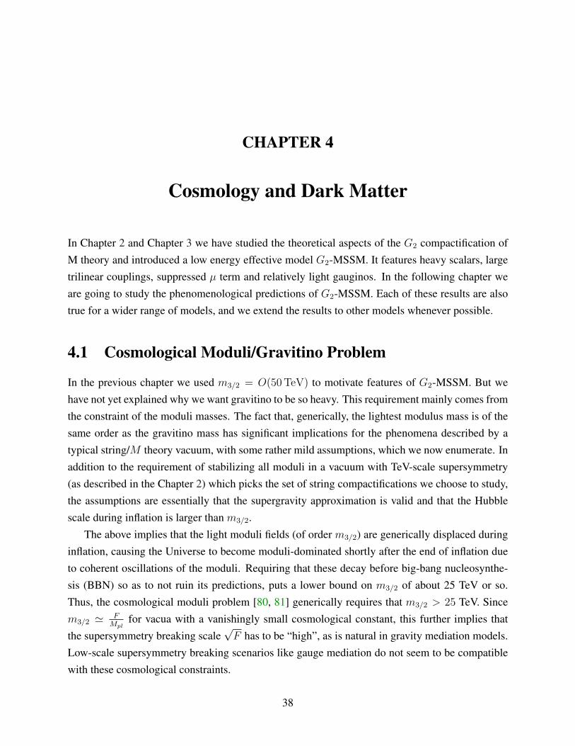
CHAPTER 4

Cosmology and Dark Matter

In Chapter 2 and Chapter 3 we have studied the theoretical aspects of the G2 compactification ofM theory and introduced a low energy effective model G2-MSSM. It features heavy scalars, largetrilinear couplings, suppressed µ term and relatively light gauginos. In the following chapter weare going to study the phenomenological predictions of G2-MSSM. Each of these results are alsotrue for a wider range of models, and we extend the results to other models whenever possible.

4.1 Cosmological Moduli/Gravitino Problem

In the previous chapter we used m3/2 = O(50 TeV) to motivate features of G2-MSSM. But wehave not yet explained why we want gravitino to be so heavy. This requirement mainly comes fromthe constraint of the moduli masses. The fact that, generically, the lightest modulus mass is of thesame order as the gravitino mass has significant implications for the phenomena described by atypical string/M theory vacuum, with some rather mild assumptions, which we now enumerate. Inaddition to the requirement of stabilizing all moduli in a vacuum with TeV-scale supersymmetry(as described in the Chapter 2) which picks the set of string compactifications we choose to study,the assumptions are essentially that the supergravity approximation is valid and that the Hubblescale during inflation is larger than m3/2.

The above implies that the light moduli fields (of order m3/2) are generically displaced duringinflation, causing the Universe to become moduli-dominated shortly after the end of inflation dueto coherent oscillations of the moduli. Requiring that these decay before big-bang nucleosynthe-sis (BBN) so as to not ruin its predictions, puts a lower bound on m3/2 of about 25 TeV or so.Thus, the cosmological moduli problem [80, 81] generically requires that m3/2 > 25 TeV. Sincem3/2 ' F

Mplfor vacua with a vanishingly small cosmological constant, this further implies that

the supersymmetry breaking scale√F has to be “high”, as is natural in gravity mediation models.

Low-scale supersymmetry breaking scenarios like gauge mediation do not seem to be compatiblewith these cosmological constraints.

38

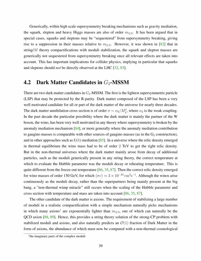
Generically, within high scale supersymmetry breaking mechanisms such as gravity mediation,the squark, slepton and heavy Higgs masses are also of order m3/2. It has been argued that inspecial cases, squarks and sleptons may be “sequestered” from supersymmetry breaking, givingrise to a suppression in their masses relative to m3/2. However, it was shown in [82] that instring/M theory compactifications with moduli stabilization, the squark and slepton masses aregenerically not sequestered from supersymmetry breaking once all relevant effects are taken intoaccount. This has important implications for collider physics, implying in particular that squarksand sleptons should not be directly observed at the LHC [32, 83].

4.2 Dark Matter Candidates in G2-MSSM

There are two dark matter candidates inG2-MSSM. The first is the lightest supersymmetric particle(LSP) that may be protected by the R-parity. Dark matter composed of the LSP has been a verywell motivated candidate for all or part of the dark matter of the universe for nearly three decades.The dark matter annihilation cross section is of order σ ∼ α2/M

2χ, where α2 is the weak coupling.

In the past decade the particular possibility where the dark matter is mainly the partner of the Wboson, the wino, has been very well motivated in any theory where supersymmetry is broken by theanomaly mediation mechanism [84], or more generally where the anomaly mediation contributionto gaugino masses is comparable with other sources of gaugino masses (as in the G2 construction),and in other approaches such as U(1) mediation [85]. In a universe where the relic density emergedin thermal equilibrium the wino mass had to be of order 2 TeV to get the right relic density.But in the non-thermal universes where the dark matter mainly arose from decay of additionalparticles, such as the moduli generically present in any string theory, the correct temperature atwhich to evaluate the Hubble parameter was the moduli decay or reheating temperature. This isquite different from the freeze-out temperature [86, 35, 87]. Then the correct relic density emergedfor wino masses of order 150 GeV, for which 〈συ〉 ' 3× 10−24 cm3s−1. Although the winos arisecontinuously as the moduli decay, rather than the superpartners being mainly present at the bigbang, a ”non-thermal wimp miracle” still occurs when the scaling of the Hubble parameter andcross section with temperature and mass are taken into account [86, 35, 87].

The other candidate of the dark matter is axions. The requirement of stabilizing a large numberof moduli in a realistic compactification with a simple mechanism naturally picks mechanismsin which many axions1 are exponentially lighter than m3/2, one of which can naturally be theQCD axion [88, 89]. Hence, this provides a string theory solution of the strong-CP problem withstabilized moduli and axions, and also naturally predicts an O(1) fraction of Dark Matter in theform of axions, the abundance of which must now be computed with a non-thermal cosmological

1the imaginary parts of the complex moduli

39

history [88].

4.3 The non-thermal WIMP ‘Miracle’

Compactified string/M theory generically gives rise to moduli fields in the effective low energydescription of physics. These are the low energy manifestations of the extra dimensions presentin string/M theory and are necessarily present as long as the supergravity approximation is valid.Moduli fields couple gravitationally universally to matter with interactions suppressed by a largescale, such as the GUT or Planck scale. They generically will dominate the energy density of theUniverse after inflation but must decay before big-bang nucleosynthesis (BBN). When they decay,they not only dilute the density of any thermal relics by many orders of magnitude, but they alsoproduce WIMPs as decay products.

This gives rise to a WIMP number density of order :

nχ ∼ΓX〈σ v〉totχχ

∼ H(TR)

〈σ v〉totχχ(4.1)

where TR is the reheat temperature generated when the modulus X decays, ΓX the modulus decaywidth and H(T ) the Hubble scale at temperature T . By contrast, in the thermal case, nthermalχ ∼H(TF )〈σ v〉totχχ

, where TF is the WIMP freezeout temperature. This implies that to obtain a roughly correctabundance in the non-thermal case, 〈σ v〉totχχ has to be larger compared to that for the thermal caseby a factor of TF

TR. Finally, within the framework of supersymmetry there naturally exist WIMP LSP

candidates like the Wino or the Higgsino with annihilation cross-sections precisely in the requiredrange. Since Winos have a larger annihilation cross-section than Higgsinos for the same mass, aWino-like LSP with a small Higgsino component is favored2.

In the next section, we describe an approach which satisfies all the conditions required for the“non-thermal WIMP miracle” to work, and which also gives rise to Wino-like LSPs in a largeregion of parameter space. Henceforth, we will study this case in detail.

4.4 Indirect Detection

Indirect Detection experiments are designed to search for particles that are potentially producedby the annihilation/decay of the dark matter in our galaxy. How does one learn what physicsinterpretation to give to tentative signals of antimatter and gammas in the galaxy? Could it bedue to annihilating dark matter? Answering this is not straightforward – it strongly depends on

2For simplicity, we do not consider models beyond the MSSM.

40

assumptions that are not always made explicit, and the answer is also very sensitive to assumptionsabout propagation in the galaxy, and to parameters used to describe the propagation. Perhapssurprisingly, assumptions about cosmological history are crucial. It also depends on whether morethan one mechanism is providing the signals.

As the recent PAMELA [1], Fermi [5] and then AMS-02 satellite data [2] appeared, essentiallyeveryone who studied it assumed that the universe cooled in thermal equilibrium after the bigbang (dark matter particles χ annihilated into Standard Model particles, which could annihilateback into dark matter particles if they had enough energy, until the cooling led to freeze-out ofthe dark matter at some relic density). Then the relic density is ρ ≈ H/〈σv〉, where the Hubbleparameter H is evaluated at the freeze-out temperature (about Mχ/25). This remarkable formula,with the relic density depending only on the cosmological Hubble parameter and on the weak scaleannihilation rate, has been called the ”wimp miracle”. Getting the correct relic density implied that〈συ〉 ≈ 3× 10−26 cm3s−1, so any candidate with a larger annihilation cross section was excluded.In recent years, however, it has become increasingly clear that comprehensive underlying theorieswhich explain more than one thing at a time generically have additional sources of dark matter,such as decaying particles, and therefore that assuming thermal equilibrium as the universe coolsis oversimplified and misleading. This was noticed in [90, 91, 92], emphasized a decade ago byMoroi and Randall[86], and more recently documented in detail in a model based on a string theoryconstruction with M theory compactified on a manifold with G2 holonomy[35]. See also [87].

Further, the standard assumption of most studies was that a single candidate had to describe thedata for electrons, positrons, antiprotons, and gammas at all energies. It’s not clear why one wouldassume that, since in the presence of dark matter there will in general be contributions from theannihilating dark matter, and also from several astrophysical sources such as interstellar mediumaccelerated by supernova remnant shock waves, pulsars, and perhaps more. In some theories thedark matter is metastable, its decay induced by much higher dimension operators, and contributesboth via annihilation and via decay (work in progress)

Remarkably, this 150 GeV mass scale is just the one that is right for the PAMELA data. In auniverse where the relic density arises non-thermally, as generically in string theories, a wino LSPwith relic density normalized to the observed local relic density (0.3 GeV/cm3) gives about theamount of positrons and antiprotons (and their distributions) reported in the PAMELA experiment!No “boost factor” is needed.

Positrons and antiprotons have long resident times in the galaxy, millions of years. In orderto compute the number of events as functions of energy that PAMELA and Fermi should observeone needs to include all the effects of propagation in the galaxy. There are two main programsto facilitate that, GALPROP[93] and DarkSUSY[94, 95], each valuable for somewhat differentcalculations. Here we use GALPROP since we need to have one program that treats the signal

41

and background particles in a self-consistent manner as they are affected by the galactic magneticfields, lose energy by synchrotron radiation, inverse Compton scattering, collisions, escape thegalactic disk, etc. As we will explain, this is crucial for understanding the antiprotons, where weargue that use of parameterized backgrounds has led people incorrectly to assume that PAMELAwas not seeing an annihilation signal in antiprotons.

We find that in the PAMELA region the results can depend significantly on a number of as-trophysical parameters (see Table 4.1), and that there are many degeneracies and flat directionsamong the parameters. The GALPROP running time is long, of order several hours, so we havenot yet been able to do full parameter scanning. Improved computing, and additional constraintsfrom satellite data that should be reported in the next few months, should improve this situationsignificantly. It should be emphasized that the positrons and antiprotons ”injected” into the galaxyby pure wino annihilation have no parameters apart from the mass scale, which can only vary atthe 5-10% level. All the issues about describing the data arise from the propagation.

If annihilation of LSP dark matter is the origin of the excess positrons, it obviously must giveexcess antiprotons since all MSSM states will include quarks and antiquarks in their annihilationproducts, and the antiquarks fragment into antiprotons. In particular, for the wino LSP the annihi-lation of winos is to W+ + W−, and the W-bosons have known branching ratios to leptonic andquark final states, and the probability they will give antiprotons was measured at LEP. The relevantprocesses are incorporated into PYTHIA and we use them. There is no freedom. This has led tomany statements in literature that the apparent absence of an antiproton excess excludes MSSMLSP models, and in particular excludes wino annihilation as the explanation of the positron excess,and forces one to approaches that only give leptons. It turns out that these conclusions are wrong,for three interesting reasons. First, the antiproton spectrum from quark fragmentation is significantdown to quite soft antiprotons, and it gives a significant number of antiprotons in the 1 − 10 GeV

region and even below. The positron spectrum from W’s has many energetic positrons at higherenergies, and is peaked at higher energies than the antiproton spectrum. Second, the antiprotonsdo not lose much energy as they propagate compared to the positrons, so the GeV antiprotons aredetected by PAMELA, while the positrons lose energy readily and the soft ones do not make it tothe detector. This can be seen from the figures below, where the signal from antiprotons is abovethe background down to the lowest energies, while the positron signal is at the background levelbelow about 5 GeV, and essentially gone below 10 GeV. Thus the positron spectra for signal andbackground have different shapes, while the antiproton spectra have essentially the same shape andmainly differ in normalization.

The third issue concerns how the background is defined. The “background” can only be de-fined if one either has data in a region where there is known to be no signal, or if one has a theoryof the background. There are two points. Some time ago reference [96] showed that solving the

42

propagation equations allowed a rather large variation in the antiproton background normaliza-tion, about a factor of five for parameters that were consistent with other constraints such as theBoron/Carbon ratio. This has also been emphasized by [96, 97]. Low energy data for antiprotonshas existed for over a decade[98, 99, 100]. People proceeded by fitting the antiproton data anddefining the fit as the background. Then they compared the PAMELA data with such backgrounds,and of course concluded there was no signal, because the signal had already been included in thebackground! If a dark matter annihilation contribution was included, it was double counted! Aswe show below, for entirely reasonable GALPROP parameters one can self-consistently computethe antiproton background, and with a wino annihilation signal it gives a good description of thedata. Consequently the early experiments such as BESS and HEAT did detect dark matter viaantiprotons.

There is another effect that has been neglected so far in most interpretations of the PAMELAand Fermi data. Dark matter annihilation is proportional to the square of the relic density. Becausegalaxies are built from smaller galaxies, and also because of normal random density fluctuations,the relic density throughout the relevant parts of the galaxy for a given observable will not be a flat0.3 GeV/cm3, but will vary. Since 〈ρ2〉 − 〈ρ〉2 6= 0, density fluctuation effects must occur. Initialstudies have been done by several authors[101, 102], who have established that the effects differfor positrons and for antiprotons, and are energy dependent, because the energy loss mechanismsare significantly different for positrons and antiprotons. While it is not clear yet how to calculateaccurately the sizes and energy dependences of these effects, it is likely that assuming no effect isa less good approximation than initial approximate calculations of the effects. We include smalleffects we estimate semi-analytically and show results with and without them. Ultimately it willbe very important to learn how to calculate these effects well and include them.

The positron data below 10 − 15 GeV is not consistent among experiments, and is not welldescribed by models. This is assumed to be due to charge-dependent solar modulation effects andis being actively studied by experts in that area, and by the experimenters [103]. We do not attemptto put in detailed corrections for this, but we do include the (non-charge-dependent) effects in thesimulation. Results in general also depend on the profile of the dark matter in the galaxy, mostimportantly for gammas from the galactic center. We do not study this dependence much heresince it does not much affect the positron and antiproton results, and we are computer-limited. Weremark on it in context below.

The PAMELA experiment has reported deviations from expected astrophysics for positrons,and as we explained above, for antiprotons, below about 100 GeV. In this paper our goal is todemonstrate that a wino LSP is a strong candidate for explaining these deviations. We assume thatpossible astrophysical sources can be added to give a complete description of the data includingFermi (which light wino annihilation obviously cannot explain). We only parameterize the higher

43

energy astrophysical part, and assume it can be accommodated by some combination of acceler-ation of the interstellar medium electrons by supernova remnant shock waves, pulsars, etc with anet e+/e− ratio of 1/3. Once we do that we make a number of predictions for the positron ratioand antiprotons at energies above those already reported, for diffuse gammas and gammas fromthe galactic center, and for gamma fluxes from dwarf galaxies in our galactic halo. We check con-straints from synchrotron radiation and ”WMAP” haze. Our prediction for gammas assumes thesource of higher energy e+ + e− does not also produce a significant flux of high energy gammas.So corrections may be needed here, but the gammas from wino annihilation will be an irreduciblesource.

We also do not criticize any other attempt to describe the data – in nearly all cases forthcom-ing PAMELA and Fermi data will favor one or another approach. Many are based on interestingideas and models. While some predictions are very sensitive to propagation effects, others suchas whether the positron ratio rises or falls above 100 GeV is not very sensitive to propagation anddifferent models have very different predictions. We predict a fall or flattening (depending some-what on the high energy astrophysical component), while most models predict a strong rise. Whilepropagation uncertainties do not modify our qualitative predictions, it is clear that the presence ofthe rather hard contribution to the e+ + e− flux introduces uncertainty in our predictions, since itcould affect the positron ratio at lower energies, and it might or might not contribute to antiprotonand gamma fluxes. As described below, we simply parameterize it and we assume it only con-tributes to the electrons and positrons, and that it contains mostly electrons (e+/e− = 1/3). Thislimits the quality of our predictions.

In the following we first describe our use of GALPROP in some detail, including some effectsor constraints we incorporate. Then we show the data and a description of the data based on anni-hilation of 180 GeV dark matter winos plus cosmic ray backgrounds, with signal and backgroundscomputed in a consistent manner. What we show is not a fit to data but merely educated guessessince the computing time for a full parameter scan is still prohibitive for us. As shown in Table 4.1below, we vary eight GALPROP parameters and some others, and all of them affect the interpre-tation. We have established that comparable descriptions of the data can be obtained for differentGALPROP parameters from those we show since there are degeneracies. We emphasize that ourgoal is to show that the wino LSP in the mass range of order 200 GeV is a good candidate forthe dark matter of the universe, including theoretical and experimental information as well as it ispossible today. Even though much is not known about the propagation of the electrons, positrons,antiprotons and gammas, quite a lot is known. Then we describe the contribution we arbitrarilyassume for the higher energy electrons and positrons. We will report on studies of the GALPROPparameter degeneracies and the wino mass later, assuming our predictions for the positron andantiproton higher energy data are correct.

44

After that we turn to presenting the data and the descriptions. We do that for one mass and oneset of propagation parameters, and one dark matter profile (NFW). Descriptions and predictionsfor higher energies are shown for the PAMELA positron excess, the PAMELA antiproton excess,the e+ + e− sum, the diffuse gammas, the gammas from the galactic center, dwarf galaxies, andchecks such as the Boron/Carbon ratio.

4.4.1 GALPROP Parameters

We use GALPROP v50.1p[93] to simulate the propagation of both cosmic rays and dark matterannihilation products in the galaxy in a consistent way. The rates and spectrum for both will changeif the propagation parameters change. The propagation process is described by the propagationequation for the particle density ψ:

∂ψ

∂t= q (~r, p) + ~∇ ·

(Dxx

~∇ψ − ~V ψ)

+∂

∂pp2Dpp

∂

∂p

1

p2ψ

− ∂

∂p

[pψ − p

3

(~∇ · ~V

)ψ]− 1

τfψ − 1

τrψ, (4.2)

where Dxx is the diffusion constant which is determined by:

Dxx = βD0xx

( RR0

)δ, (4.3)

where β is the velocity of the particle, R is the particle rigidity, and R0 is the reference rigiditywhich is taken to be 4 GV in all the simulations. In order to consider the propagation of the darkmatter signals in the same framework, the official GALPROP code is modified to accept the darkmatter injection spectrum calculated using PYTHIA via DarkSUSY 5.0.4[94]. The parametersused in this paper are based on the conventional model with constant Xco-factor provide in GAL-PROP source code (galdef 50p 599278). In general we vary the parametersDxx, δ , the half heightof the diffusion zone zh, the primary electron injection index γ0, the normalization of the primaryelectron flux Ne− , the scaling factor for inverse Compton scattering, the convection velocity Vc,and the Alfven velocity Va. We survey ranges of these parameters (but do not fit data or scanparameters because of computing limitations) in order to learn if a combination of conventionalcosmic ray physics plus dark matter annihilation can give a reasonable description of the PAMELAand Fermi data within certain constraints such as the B/C ratio described further below.

We find a set of parameters that give a good description of the data, and those are used in thefigures below except when stated otherwise.The half height of the diffusion zone zh = 2 kpc.The diffusion coefficient is D0xx = 2.5 × 1028 cm2s−1, δ = 0.5. We also assume a softer

45

GALPROP ParametersDxx0 (cm2s−1) 2.5× 1028

δ 0.5R0 (GV) 4zh (kpc) 2γ0 2.6

Ne− (cm−2s−1sr−1MeV−1) 2.88× 10−10

Vc (kms−1kpc−1) 5Va (kms−1) 31

ISRF factors (optical, FIR, CMB) 0.5, 0.5, 0.5Solar Modulation Parametersφ (MV) 500pc (GeV) 1

Astrophysical Flux Parametersa 1.0b 1.8

z0 (kpc) 0.2γ 1.5

M (GeV) 950Density Fluctuation Factor Parameters

Bc 2.5f 0.5

Table 4.1: The parameters used for simulation. The physical meaning of these parameters isdescribed in the text.

primary electron injection spectrum by setting the injection index γ0 for primary electrons be-tween 4 GeV to 106 GeV to 2.6. Also the primary electron flux is normalized to Ne− = 2.88 ×10−10 cm−2sr−1s−1MeV−1 at 34.5 GeV. The scaling factors for inverse Compton (ISRF factor)are adjusted to 0.5, which is approximately equivalent to setting τ = 2× 1016 s in the energy lossrate formula for electron b (ε)e± = 1

τε2. The convection velocity is Vc = 5 km s−1kpc−1, and the

Alfven speed which determines the reacceleration process is Va = 31 km s−1. The summary of theparameters we are using can be found in Table 4.1. Other parameters not mentioned here are thesame as galdef 50p 599278.

As described in the introduction, the dark matter we focus on is the theoretically well-motivatedcase of a pure wino LSP, which annihilates to W ’s: W + W → W+ + W−. The dark matterinjection parameters are then completely determined by the wino mass and W± decays.

46

4.4.2 Solar Modulation

The effect of solar modulation is estimated by the Force-Field approximation [104], The flux ob-served at Earth’s orbit JE (ε) is related to the flux in the interstellar flux by the following relation:

JE (ε) =ε2 −m2

ε2∞ −m2

J∞ (ε∞) (4.4)

where ε∞ is the energy of the corresponding interstellar flux, which is determined by:

ε∞ =

{p log

(pc+εcp+ε

)+ ε+ Φ ε < εc

ε+ Φ ε ≥ εc(4.5)

Φ is the modulation energy shift which can be calculated from the modulation potential Φ = |Z| eφ,In our simulation the modulation potential φ is 500 MV, the reference momentum pc is 1 GeV.Only the solar modulation effect for electron/positron and antiproton/proton is considered in thiswork. These effects do not include charge dependent solar modulation, which is under study [103]

47

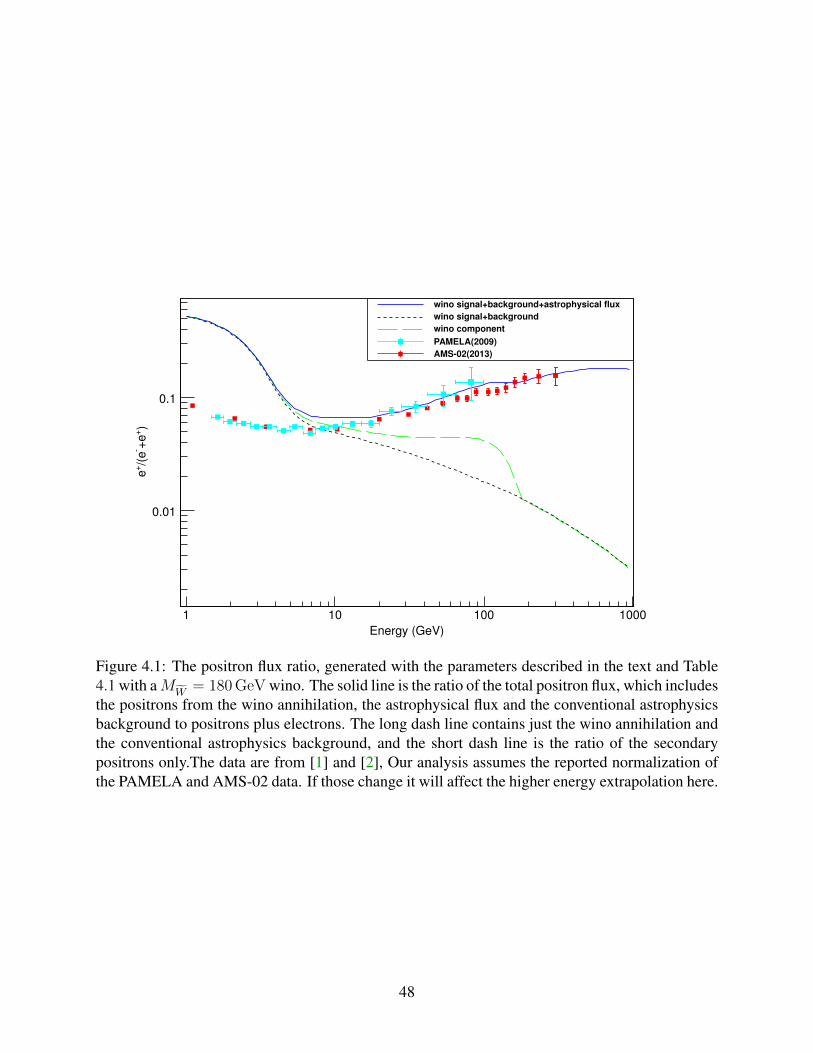
Energy (GeV)

1 10 100 1000

)+

+e

­/(

e+

e

0.01

0.1

wino signal+background+astrophysical flux

wino signal+background

wino component

PAMELA(2009)

AMS­02(2013)

Figure 4.1: The positron flux ratio, generated with the parameters described in the text and Table4.1 with aMW = 180 GeV wino. The solid line is the ratio of the total positron flux, which includesthe positrons from the wino annihilation, the astrophysical flux and the conventional astrophysicsbackground to positrons plus electrons. The long dash line contains just the wino annihilation andthe conventional astrophysics background, and the short dash line is the ratio of the secondarypositrons only.The data are from [1] and [2], Our analysis assumes the reported normalization ofthe PAMELA and AMS-02 data. If those change it will affect the higher energy extrapolation here.

48

Kinetic Energy (GeV)

1 10 100 1000

)p

/(p

+p

­510

­410

wino signal(with dff)+background

wino signal+background

background

PAMELA

Figure 4.2: The antiproton flux ratio. The solid line is the ratio of the total antiproton flux, whichinclude the antiproton from wino annihilation, and conventional astrophysics background, the dashline has the same components but without the density fluctuation factor, the dot line is astrophysicsbackground only. The data are from PAMELA [3]. Note the signal is larger than the backgrounddown to very low energies.

49

Kinetic Energy (GeV/nuc)

0.1 1 10 100 1000

B/C

Rati

o

0.05

0.1

0.15

0.2

0.25

0.3

0.35GALPROP

HEAO

(A)

Figure 4.3: The Boron to Carbon ratio with our standard parameters, solar modulation effect is notincluded, The data are from [4].

50

Kinetic Energy (GeV/nuc)

0.1 1 10 100 1000

B/C

Rati

o

0.05

0.1

0.15

0.2

0.25

0.3

0.35GALPROP

HEAO

(B)

Figure 4.3: The Boron to Carbon ratio with one parameter different (δ changes from 0.5 to 0.4).This illustrates that the Boron to Carbon ratio is very sensitive the diffusion parameters. The dataare from [4].

51

4.4.3 Astrophysical Flux

It is obvious that a 180 GeV wino alone cannot explain Fermi date and PAMELA data at the sametime. There must be some extra flux responsible for the high energy signals. In order to estimatethe high energy (> 200 GeV) electrons/positrons flux, we consider a simple model for extra fluxwhich is suggested by interstellar medium electrons accelerated by supernova remnants and shockwaves, or by pulsar spectra models. The basic setup we use is similar to Zhang and Cheng[105].For a recent review of pulsar models, see Profumo[106]. The spatial distribution of the sources is:

ρ (r) = N

(r

r�

)ae− b(r−r�)

r� e− zz0 (4.6)

where N is the overall normalization constant, z0 = 0.2kpc, r� = 8.5kpc, a = 1.0 and b = 1.8.The energy dependence of the injection spectrum is:

dNe±

dE= N ′E−γe−

EM (4.7)

where N ′ is another normalization constant, which can be absorbed into N , γ = 1.5 and M =

950 GeV. In order to fit PAMELA and Fermi data, we made an ad hoc assumption that the ratioof positron and electron in the unknown extra flux is 1 : 6. The high energy positrons/electronsare then propagated by GALPROP, and the resulting flux is normalized to fit the Fermi data byrequiring the extra electron flux at 275.5 GeV to be 3.0× 10−13 cm−2sr−1s−1MeV−1

4.4.4 Density Fluctuation Factor

The results from N-body simulations [107], and an understanding of how galaxies formed, indicatethat it is inevitable for the dark matter halo of our galaxy to have substructures. The existence ofthese substructures would change the predictions of the cosmic ray fluxes, particularly for darkmatter annihilation. Even without substructures, it is clear that the density of dark matter will notbe absolutely flat, but will fluctuate around an average value. Both of these effects require the fluxfrom dark matter annihilation, which is sensitive to the square of the dark matter density, to showdensity fluctuation effects. As emphasized by Lavalle and collaborators[101, 102], the effects ofthese substructures are different for positrons and antiproton, and must also be energy dependent.The details of these effects depend on the spatial and mass distribution of these substructures. Herewe use a very simple model to estimate the effects: Assuming all the substructures share the samemass and density, and the spatial number density of the substructures is proportional to the densityprofile of the smooth distribution of dark matter halo.

52

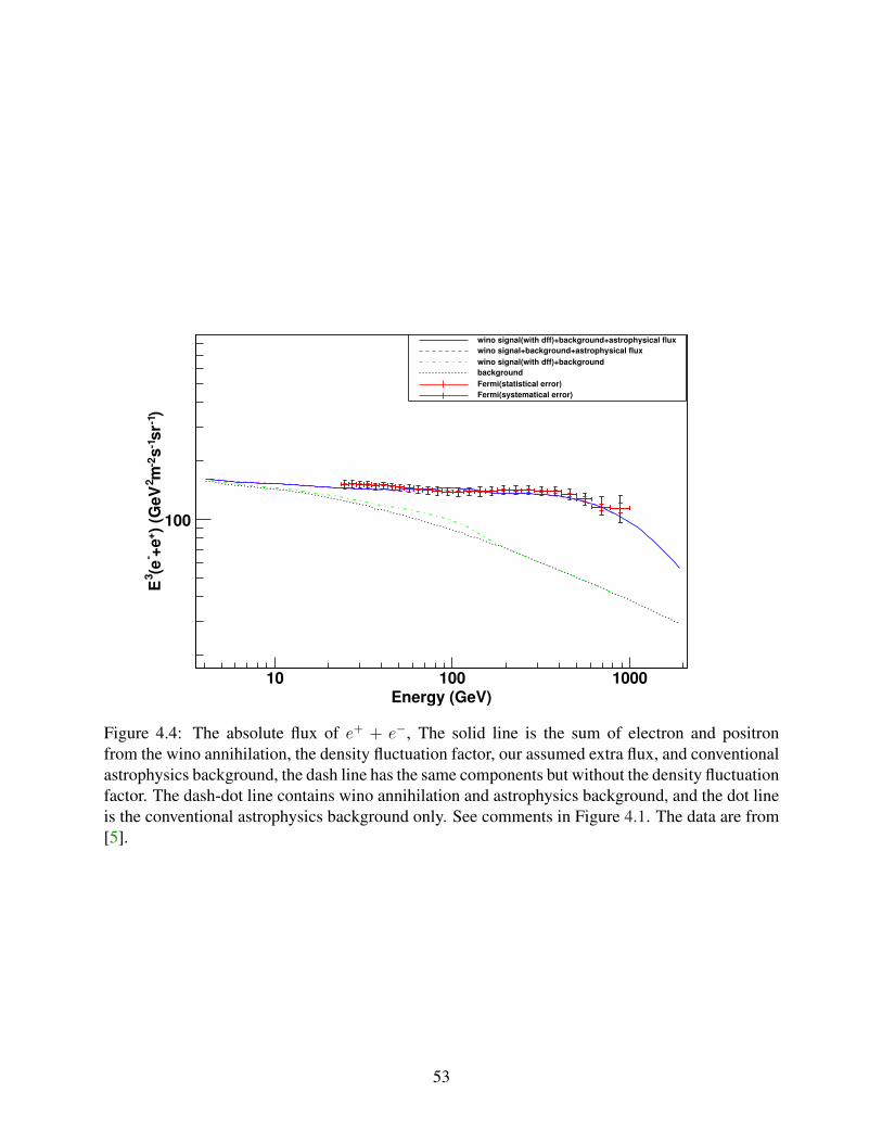
Energy (GeV)10 100 1000

)­1

sr

­1s

­2m

2)

(GeV

++

e­

(e3

E

100

wino signal(with dff)+background+astrophysical flux

wino signal+background+astrophysical flux

wino signal(with dff)+background

background

Fermi(statistical error)

Fermi(systematical error)

Figure 4.4: The absolute flux of e+ + e−, The solid line is the sum of electron and positronfrom the wino annihilation, the density fluctuation factor, our assumed extra flux, and conventionalastrophysics background, the dash line has the same components but without the density fluctuationfactor. The dash-dot line contains wino annihilation and astrophysics background, and the dot lineis the conventional astrophysics background only. See comments in Figure 4.1. The data are from[5].

53

With these assumptions, the density fluctuation factor can be calculated with:

D (E) = (1− f)2 + fBcI1

I2

(4.8)

where f is the mass fraction of the substructures in the dark matter halo, Bc is the intrinsic densityincrease of the substructures or fluctuations, and In is determined by

In =

∫DM halo

G (x,E)

{ρs (x)

ρ0

}nd3x (4.9)

where G (x,E) is the Green’s function of the propagating particle.We assume f = 0.5 and Bc = 2.5. Only the density fluctuations of positron and antiproton

are considered. The electron/positron Green’s function from Baltz and Edsjo[108] and the fastformulae for antiproton Green’s function from Maurin, Taillet and Combet[109] are used to eval-uate the integral. With these assumptions we find the effects of the density fluctuations are small.We included them for completeness. Theory curves including them are labeled “dff” (for “densityfluctuation factors”) in the figures.

4.5 Direct Detection

Direct detection experiments of dark matter are based on the detection of collisions between thedark matter particle and the nuclei. In contrast to the large annihilation cross section, a pure winohas a very small direct detection cross section, which makes the direct detection searches for winoLSP dark matter extremely challenging.

In the decoupling limit, defined when the pseudoscalar mass is much larger that the Z-bosonmass, mA0 � MZ , the charged and heavy CP-even Higgses are also heavy, mH± ' mH0 ' mA0 .The other Higgs boson h0 remains light and behaves in the same way as the SM Higgs boson. Herewe will assume its mass is 125 GeV. Since the squarks are also heavy inG2-MSSM, the light Higgsboson exchange will give the only substantial contribution to the spin-independent scattering crosssections. The scattering of the LSP off nuclei is via the Higgsino and gaugino component. Whilethe LSP will be mostly Wino-like, the prediction that µ is of order the TeV scale implies that theLSP wavefunction can have non-trivial Higgsino mixing.

Following [110] we estimate the size of the direct detection cross section in the decoupling

54

limit to be

σSI (χN → χN) ≈ 3.6× 10−45cm2

(125 GeV

mh

)4(ZHu sin β − ZHd cos β

0.1

)2

× (ZW − tan θWZB)2 (4.10)

where the Z’s give the composition of the LSP

χ ≡ ZB B + ZW W + ZHd Hd + ZHu Hu. (4.11)

This gives us an estimate of the largest direct detection scattering cross sections, which naivelymay seem that for ZHu ∼ 0.1 can be very close to the reach of XENON. Eq. (4.10) can further besimplified, with the aid of analytical expressions for the neutralino mass matrix eigenvalues andeigenvectors [111, 112, 113]. Taking the limit M1 = M2, which maximizes the scattering crosssection for fixed µ and tanβ, (4.10) becomes

σMSSMSI (χN → χN) ≈ 4.3× 10−45cm2

(125 GeV

mh

)4(1 TeV

µ

)2(sin 2β +M2/µ

1− (M2/µ)2

)2

(4.12)

which falls off both with tanβ and µ. Allowing for the variation in M1 and M2 in the G2-MSSMwill only decrease this fraction. The value M2/µ is typically around .1 ∼ .2. For general MSSM,sin 2β can be almost 1, corresponding to a very small tan β. For G2-MSSM, as mentioned in theprevious chapter, tan β ∼ 10, which makes sin 2β ∼ 0.1. So the upper limit of the direct detectioncross section for G2-MSSM is about 10−47cm2

55

CHAPTER 5

The Mass of the Lightest Higgs Particle

5.1 Higgs Mass Calculation

Most physicists agree that understanding the origin of electroweak symmetry breaking is essentialfor progress in going beyond the Standard Model. We will demonstrate that, with some broad andmild assumptions motivated by cosmological constraints, generic compactified string/M -theorieswith stabilized moduli and low-scale supersymmetry imply a Standard Model-like single Higgsboson with a mass 105 GeV . Mh . 129 GeV if the matter and gauge spectrum surviving belowthe compactification scale is that of the MSSM, as seen from Figure 5.1. For an extended gaugeand/or matter spectrum, there can be additional contributions to Mh. Furthermore, in G2-MSSMmodels we find that the range of possible Higgs masses is apparently much smaller, For 30 TeV .

m3/2 . 100 TeV, which is consistent with cosmology and dark matter observations, 122 GeV .

Mh . 129 GeV. When we choose m3/2 = 50 TeV, the mass is 126± 1.5 GeV.In connecting string/M theory to low-energy particle physics, one has to compactify the extra

dimensions. Motivated by grand unification and its successful embedding into string/M theorywe assume that the string/M theory scale, the Kaluza-Klein scale and the unification scale areall within an order of magnitude of 1016 GeV. Within the theoretical precision desired, numericalresults for Mh are not sensitive to variations of an order of magnitude or so in these scales.

We will be interested in models with supersymmetry breaking mechanisms which give rise toTeV-scale supersymmetry, and hence solve the naturalness problems in the Standard Model. Thebasic mechanisms were described in [28, 29] for M -theory and in [114, 115, 89] for Type IIBcompactifications, where it was shown that all moduli can be stabilized and supersymmetry canbe broken with ∼ TeV-scale superpartners with a natural choice of parameters - in which the onlydimensionful scale is Mpl! In a vacuum with broken supersymmetry and vanishing cosmologicalconstant, the mass of the gravitino (m3/2), which is the superpartner of the massless graviton, isthe order-parameter of supersymmetry breaking and sets the mass scale for all superpartners andalso indirectly the Higgs mass.

56

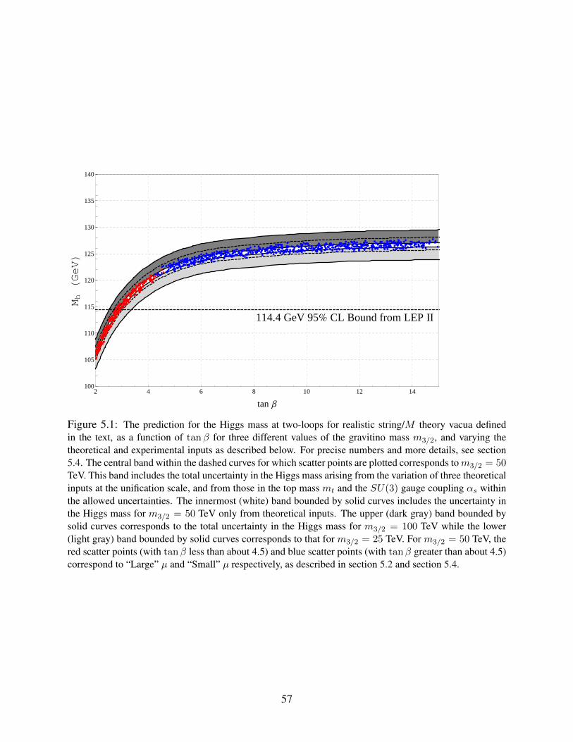
2 4 6 8 10 12 14100

105

110

115

120

125

130

135

140

tan Β

Mh

HGe

VL

114.4 GeV 95% CL Bound from LEP II

Figure 5.1: The prediction for the Higgs mass at two-loops for realistic string/M theory vacua definedin the text, as a function of tanβ for three different values of the gravitino mass m3/2, and varying thetheoretical and experimental inputs as described below. For precise numbers and more details, see section5.4. The central band within the dashed curves for which scatter points are plotted corresponds tom3/2 = 50TeV. This band includes the total uncertainty in the Higgs mass arising from the variation of three theoreticalinputs at the unification scale, and from those in the top mass mt and the SU(3) gauge coupling αs withinthe allowed uncertainties. The innermost (white) band bounded by solid curves includes the uncertainty inthe Higgs mass for m3/2 = 50 TeV only from theoretical inputs. The upper (dark gray) band bounded bysolid curves corresponds to the total uncertainty in the Higgs mass for m3/2 = 100 TeV while the lower(light gray) band bounded by solid curves corresponds to that for m3/2 = 25 TeV. For m3/2 = 50 TeV, thered scatter points (with tanβ less than about 4.5) and blue scatter points (with tanβ greater than about 4.5)correspond to “Large” µ and “Small” µ respectively, as described in section 5.2 and section 5.4.

57

A natural prediction of such compactifications is that the mass of the lightest modulus is closeto m3/2. In fact, this is a generic result for compactified string/M -theories with stabilized moduliwithin the supergravity approximation. In vacua in which the superpotential W is not tuned, itessentially arises from the fact that there is a relationship between the dynamics stabilizing themoduli and the dynamics breaking supersymmetry due to the extremely tiny value of the cosmo-logical constant. Thus, the modulus mass becomes related to the gravitino mass. For more details,see [116, 117, 118, 119, 120, 121]. For the generic case with many moduli, at least some of themoduli are stabilized by perturbative effects in the Kahler potential [29, 89]. Then, it can be shownthat the lightest modulus1 has a mass of the same order as m3/2 [122, 32].

5.2 The Higgs and BSM Physics

We are interested in calculating the Higgs mass arising from realistic compactifications satisfyingthe conditions above. In a supersymmetric theory, two Higgs doublets are required for anomalycancellation; so by the “Higgs mass” we mean the mass of the lightest CP-even neutral scalar inthe Higgs sector. A remarkable fact about the Higgs mass in general supersymmetric theories isthat an upper limit onMh of order 2MZ exists just from the requirement of validity of perturbationtheory up to the high scale of order 1016 GeV [123, 124]. This is due to the fact that the Higgsmass at tree-level only depends on SM gauge couplings (which have been measured), and possiblyother Yukawa or gauge couplings (which are bounded from above by perturbativity). However,in addition to the gauge and matter spectrum, the precise value of the Higgs mass depends cru-cially on radiative effects, which in turn depend on all the soft parameters including the µ and Bµparameters.

In this work we assume that the visible sector consists of the SM gauge group with the MSSMmatter content below the unification scale, as suggested by gauge coupling unification and radiativeEWSB in the MSSM. In addition, we consider compactifications in which the gravitino mass m3/2

is not too far above the lower bound of∼ 25 TeV from the moduli decay constraint, and the gauginomasses are suppressed by one-to-two orders of magnitude relative to m3/2. For µ we study twocases, one in which µ is suppressed by one-to-two orders of magnitude relative tom3/2 as predictedin [125], and the other in which µ is of the same order as m3/2 [56, 126, 127, 128, 129]. We denotethese two cases as “Small” µ and “Large” µ respectively. The two cases are studied as they pickout different regions of tan β and hence give different predictions for the Higgs mass as seen fromFigure 1. For more discussion, see section 5.4.

Note that only one of the five scalars in the Higgs sector of the MSSM is light, the rest are allof order m3/2. Hence, we are in the “decoupling limit” of the MSSM where the lightest CP-even

1 more precisely, the real part of the chiral superfield making up the complex modulus in the 4D theory.

58

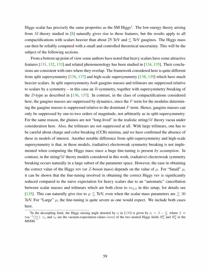
Higgs scalar has precisely the same properties as the SM Higgs2. The low-energy theory arisingfrom M -theory studied in [8] naturally gives rise to these features, but the results apply to allcompactifications with scalars heavier than about 25 TeV and . TeV gauginos. The Higgs masscan then be reliably computed with a small and controlled theoretical uncertainty. This will be thesubject of the following sections.

From a bottom up point of view some authors have noted that heavy scalars have some attractivefeatures [131, 132, 133] and related phenomenology has been studied in [134, 135]. Their conclu-sions are consistent with ours where they overlap. The framework considered here is quite differentfrom split supersymmetry [136, 137] and high-scale supersymmetry [138, 139] which have muchheavier scalars. In split supersymmetry both gaugino masses and trilinears are suppressed relativeto scalars by a symmetry – in this case an R-symmetry, together with supersymmetry breaking ofthe D-type as described in [136, 137]. In contrast, in the class of compactifications consideredhere, the gaugino masses are suppressed by dynamics, since the F -term for the modulus determin-ing the gaugino masses is suppressed relative to the dominant F -term. Hence, gaugino masses canonly be suppressed by one-to-two orders of magnitude, not arbitrarily as in split-supersymmetry.For the same reason, the gluinos are not “long-lived” in the realistic string/M theory vacua underconsideration here. Also, the trilinears are not suppressed at all. With large trilinears, one has tobe careful about charge and color breaking (CCB) minima, and we have confirmed the absence ofthese in models of interest. Another notable difference from split-supersymmetry and high-scalesupersymmetry is that, in those models, (radiative) electroweak symmetry breaking is not imple-mented when computing the Higgs mass since a huge fine-tuning is present by assumption. Incontrast, in the string/M theory models considered in this work, (radiative) electroweak symmetrybreaking occurs naturally in a large subset of the parameter space. However, the ease in obtainingthe correct value of the Higgs vev (or Z-boson mass) depends on the value of µ. For “Small” µ,it can be shown that the fine-tuning involved in obtaining the correct Higgs vev is significantlyreduced compared to the naive expectation for heavy scalars due to an “automatic” cancellationbetween scalar masses and trilinears which are both close to m3/2 in this setup; for details see[135]. This can naturally give rise to µ . TeV, even when the scalar mass parameters are & 30

TeV. For “Large” µ, the fine-tuning is quite severe as one would expect. We include both caseshere.

2In the decoupling limit, the Higgs mixing angle denoted by α in [130] is given by α = β − π2 , where β ≡

tan−1(vuvd ). vu and vd are the vacuum-expectation-values (vevs) of the two neutral Higgs fields H0u and H0

d in theMSSM.

59

5.3 Computation of the Higgs Mass

Computing the Higgs mass in the MSSM with scalar masses and trilinears at Msusy & 25 TeV,and gauginos and µ suppressed by one-to-two orders of magnitude relative to the scalar masses, isnon-trivial. Although conceptually quite different, some of the technical issues involved have anoverlap with split-supersymmetry and high-scale supersymmetry.

Since the scalar masses are much larger than a TeV, they could lead to non-trivial quantumcorrections in the gaugino-higgsino and Higgs sectors enhanced by “large logarithms” of the ratiobetween the electroweak scale and the scalar mass scale. Many numerical codes tend to becomeless reliable for scalar masses larger than a few TeV for the above reason. However, in contrast tosplit supersymmetry and high-scale supersymmetry models, the scalar masses here are 25-100 TeVwhich is not that “large”, since log(Msusy

MEW) is not large. So, numerical codes should still provide

a reasonable estimate. The ratio of the two Higgs fields vevs, tan β cannot yet be calculatedaccurately, and significantly affects the value of Mh if tan β . 10, so we include the variationfrom tan β. This dependence actually allows an approximate measurement or useful limit ontan β which is otherwise very difficult to do.

In light of the above, we adopt the following procedure. At the unification scale around 1016

GeV, in accord with theoretical expectations we fix the soft parameters - the scalar masses equalto m3/2, the trilinears A close to m3/2, and the gaugino masses suppressed by one-to-two ordersof magnitude relative to the scalar masses as described in [8]. Then, for a given value of tan β,the numerical codes SOFTSUSY [74] and SPHENO [140] are used to renormalize these quantitiesdown to Msusy ≈ m3/2, where electroweak symmetry breaking is implemented. This determinesµ and Bµ. The quantities are chosen such that the values of µ and Bµ are consistent with thetheoretical expectations. One consequence of this is that tan β is not expected to span the fullyphenomenologically allowed range from∼ 2 to∼ 60, but only a restricted range from∼ 2 to∼ 15

[32]. In any case, from Figure 1, since the Higgs mass saturates for tan β & 12, plotting highervalues of tan β will not provide new information.

Then, we compute the Higgs mass in the “match-and-run” approach using values of gauginomasses, µ and Bµ at Msusy determined from above. We follow a procedure similar to that in [141]except that we only consider those parameters at the unification scale which after RG evolutionto Msusy give rise to viable electroweak symmetry breaking. We also compute the Higgs massdirectly with SOFTSUSY using theoretical inputs at the unification scale, and compare to theresults obtained with the “match-and-run” approach, the detailed procedure for which is describedbelow.

60

5.3.1 Matching at Msusy

At the scale Msusy, the full supersymmetric theory is matched to a low energy theory with fewerparticles, consisting of the SM particles, the gauginos and the higgsinos for the “Small” µ case,and only the SM particles and the gauginos for the “Large” µ case. The matching condition for thequartic coupling of the Higgs in the low-energy theory is given at Msusy by:

λ =1

4

[g2

2 +3

5g2

1

]cos2 2β + δλth (5.1)

where g1, g2 are the U(1)Y and SU(2)L gauge couplings evaluated at Msusy. The threshold cor-rections to the quartic coupling at one-loop consist of leading log (LL) as well as finite corrections.The above matching condition is strictly valid only in the DR scheme, so there is an additionalcorrection if one wants to convert to theMS scheme as explained in the appendix of [142]. We usethe standard choice Msusy =

√Mt1 Mt2 where Mt1 ,Mt2 are the masses of the two stop squarks,

and include all the relevant LL and finite threshold corrections. The dominant finite thresholdeffects to the Higgs quartic coupling comes from stop squarks, and is given by:

δλth ≈3 y4

t

8π2

(A2t

m2t

− A4t

12m4t

)(5.2)

Since the trilinears A are of the same order as scalars, this is a non-trivial correction when thescalars and trilinears are around 25 TeV. Other finite threshold corrections are smaller, and havebeen neglected as they do not affect the result to within the accuracy desired.

The matching conditions for the gaugino-higgsino-Higgs couplings (denoted by κ in general)at Msusy in the DR scheme are given by:

κ2u = g2 sin β; κ2d = g2 cos β;

κ1u =

√3

5g1 sin β; κ1d =

√3

5g1 cos β; (5.3)

where the gauge couplings are to be evaluated at Msusy. As for the Higgs quartic coupling, addi-tonal corrections are present in the MS scheme, which can be obtained from [142].

5.3.2 Two -loop RGEs and Weak Scale Matching

We use two-loop RGEs computed in [141] for the gauge couplings, third-generation Yukawa cou-plings yt, yb, yτ , the Higgs quartic λ, and the gaugino-higgsino-Higgs (κ) couplings (for “Small”µ), to renormalize them down to the weak scale. For “Large” µ, the κ couplings are not presentin the low-energy theory, and (5.3) is used to compute the threshold correction from higgsinos at

61

Msusy.Note that unlike the κ couplings and the quartic coupling, the boundary conditions for which are

defined at Msusy, the boundary conditions for the gauge and Yukawa couplings yb, yτ are definedat MZ - the Z-pole, while that for the top Yukawa coupling yt is defined at the top pole massmt = 173.1± 0.9 GeV [143]. In particular, the boundary values of the running gauge and Yukawacouplings in the MS scheme are extracted from experimental observables at the weak scale byincluding threshold effects, as explained in [142]. For the top Yukawa coupling yt, non-trivialthree-loop QCD corrections, and one-loop electroweak and superpartner threshold corrections arealso included as they are non-negligible and play an important role in the precise prediction for theHiggs mass.Since the boundary conditions are given at different scales, an iterative procedure isrequired to solve the coupled differential RGE equations. We follow a procedure similar to that in[141, 144, 142]. Then, the Higgs mass is given by:

Mh =√

2 v

√λ(Q) + δλ(Q) + δλ(Q) (5.4)

where v = 174.1 GeV, δλ stands for the corrections from the SM particles, and δλ stands for thecorrections from the supersymmetric fermions at the weak scale, and all couplings are evaluatedat the MS scale Q = mt. The expressions are given in [141]. Finally, as mentioned earlier, sincenumerical codes are expected to give a good estimate of the Higgs mass, we compute the Higgsmass directly with SOFTSUSY. We find very good agreement between the two results, to within 1GeV.

5.4 Result

Figure 5.1 gives the Higgs mass as a function of tan β by varying the theoretical inputs at theunification scale in ranges predicted by the theory, and mt and αs within the allowed uncertainties.The values of the Higgs mass shown are in the “match-and-run” approach. The ranges of thetheoretical and experimental inputs, and the resulting uncertainties are discussed in detail below.The µ and Bµ parameters are related by electroweak symmetry breaking to tan β, so by varyingtan β one is effectively varying µ and Bµ. As pointed out in section 5.1, theoretical considerationstypically give rise to two different classes of phenomenologically viable predictions for µ – one inwhich µ is suppressed by one-to-two orders of magnitude relative to m3/2, and the other in whichµ is comparable to m3/2. As seen from Figure 1, the two classes of predictions for µ give rise todifferent values of tan β because of the EWSB constraints that relates them; hence a measurementof the Higgs mass will not only determine or constrain tan β, it will also favor one class of µ-generating mechanisms over the other! For instance, in G2-MSSM models arising from M theory,

62

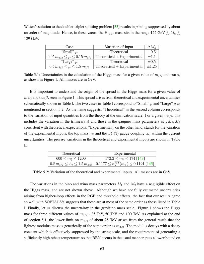
Witten’s solution to the doublet-triplet splitting problem [33] results in µ being suppressed by aboutan order of magnitude. Hence, in these vacua, the Higgs mass sits in the range 122 GeV . Mh .

129 GeV.

Case Variation of Input ∆Mh

“Small” µ Theoretical ±0.50.05m3/2 ≤ µ ≤ 0.15m3/2 Theoretical + Experimental ±1.1

“Large” µ Theoretical ±0.50.5m3/2 ≤ µ ≤ 1.5m3/2 Theoretical + Experimental ±1.25

Table 5.1: Uncertainties in the calculation of the Higgs mass for a given value of m3/2 and tan β,as shown in Figure 1. All masses are in GeV.

It is important to understand the origin of the spread in the Higgs mass for a given value ofm3/2 and tan β, seen in Figure 1. This spread arises from theoretical and experimental uncertaintiesschematically shown in Table I. The two cases in Table I correspond to “Small” µ and “Large” µ asmentioned in section 5.2. As the name suggests, “Theoretical” in the second column correspondsto the variation of input quantities from the theory at the unification scale. For a given m3/2, thisincludes the variation in the trilinears A and those in the gaugino mass parameters M1,M2,M3

consistent with theoretical expectations. “Experimental”, on the other hand, stands for the variationof the experimental inputs, the top mass mt and the SU(3) gauge coupling αs, within the currentuncertainties. The precise variations in the theoretical and experimental inputs are shown in TableII.

Theoretical Experimental600 ≤ mg ≤ 1200 172.2 ≤ mt ≤ 174 [143]

0.8m3/2 ≤ At ≤ 1.5m3/2 0.1177 ≤ αMSs (mZ) ≤ 0.1191 [145]

Table 5.2: Variation of the theoretical and experimental inputs. All masses are in GeV.

The variations in the bino and wino mass parameters M1 and M2 have a negligible effect onthe Higgs mass, and are not shown above. Although we have not fully estimated uncertaintiesarising from higher-loop effects in the RGE and threshold effects, the fact that our results agreeso well with SOFTSUSY suggests that these are at most of the same order as those listed in TableI. Finally, let us discuss the uncertainty in the gravitino mass scale. Figure 1 shows the Higgsmass for three different values of m3/2 - 25 TeV, 50 TeV and 100 TeV. As explained at the endof section 5.1, the lower limit on m3/2 of about 25 TeV arises from the general result that thelightest modulus mass is generically of the same order as m3/2. The modulus decays with a decayconstant which is effectively suppressed by the string scale, and the requirement of generating asufficiently high reheat temperature so that BBN occurs in the usual manner, puts a lower bound on

63

m3/2. Therefore, the lower limit on m3/2 is uncertain only by a small amount. Although the upperlimit is less tightly constrained, theoretical expectations constrain it to be not be much above 100TeV. This is because in the string/M theory vacua considered here, gaugino masses are suppressedonly by one-to-two orders of magnitude relative to m3/2 in accord with theoretical expectations[146, 147, 148, 149, 150, 151]. Therefore, the requirement of gauginos to be light enough (withmasses . TeV) such that they are part of the low-energy theory at Msusy as assumed in section5.3.1, puts an upper limit on m3/2 of about 100 TeV. A similar upper bound also arises in realisticmoduli stabilization mechanisms satisfying the supergravity approximation. Improvements in dataas well as theory in the future will be extremely helpful in constraining the gravitino mass.

64

CHAPTER 6

Gluino and Chargino Searches at the LHC

The generic prediction of heavy scalars in G2-MSSM makes its LHC phenomenology both chal-lenging and interesting. Since we will not be able to produce the scalar particles directly at theLHC, the gauginos will be our main window of new physics: The wino LSP will produce largemissing energy. It is possible to study signals rely solely on missing transverse energy(MET) likemonojets. Most of the time however, it is much easier to search for other gauginos in G2-MSSM.The production cross section of gluinos are not small due to the strong coupling. Gluinos decaythrough the heavy squarks, so the decay channel with the lightest squark is enhanced. InG2-MSSMthis corresponds to the decay channel containing 3rd generation squarks. This enhancement is par-tially cancelled by the small phase space when top quarks are presented in the decay product. Insummary the gluino will decay into all the quarks with similar branching fractions, with the decaychannels containing the top and bottom quarks slightly enhanced.

When the LSP is a pure wino like in the G2-MSSM, the mass of the LSP and the lightestchargino are almost degenerate. The chargino can only decay into soft leptons or pions plus theLSP. This gives the chargino an unusually long lifetime. After being produced in the LHC, it canfly several centimeters, generate signals in the tracking chamber. Then the chargino will decay intothe LSP and soft particles, effectively becomes invisible from the detector point of view.Besidesbeing another way to searching for new physics, the chargino tracks also provide unique kinematicinformation. The 3-momentum of the chargino, which is almost equal to the 3-momentum ofthe LSP, can be used to estimate the missing energy. With enough chargino tracks and extrainformation about the mass of the LSP, it might be even possible to reconstruct the entire events.

6.1 General Gluino Search Signatures

In this work we have implemented the complete analytical expressions for soft breaking terms ofthe G2-MSSM into SOFTSUSY[74]. The analysis includes the gaugino mass threshold correc-tions [70] with 2 loop scalar corrections, 2-loop RGEs for the Higgs and gaugino masses, µ, and

65

Yukawa and gauge couplings [73, 74]. Branching fractions have been computed with SUSY-HIT [152] and production of signal and backgrounds are generated with PYTHIA [153] andPGS4 [154] with the level 1 (L1) triggers designed to efficiently reproduce CMS specifications[155] (for detailed discussions see e.g. [156]). Signal and background have been simulated at√s = (7, 10, 14) TeV in order to generalize our predictions for preliminary LHC runs and fu-

ture operational center of mass energies. Specifically, SM backgrounds have been generated withQCD multi-jet production due to light quark flavors, heavy flavor jets (bb, tt), Drell-Yan, singleZ/W production in association with quarks and gluons (Z+ jets / W+ jets), and ZZ, WZ, WW

pair production resulting in multi-leptonic backgrounds. Laboriously, samples were generated at√s = (7, 10, 14)TeV with up to 5 fb−1 of luminosity. In PGS4 jets are defined through a cluster-

based algorithm which has a heavy flavor tagging efficiency based on the parametrizations of theCDF Run II tight/loose (secondary) vertex b-tagging algorithm [157]. The standard criteria forthe discovery limit of new signals is that the SUSY signals should exceed either 5

√NSM or 10

whichever is larger, i.e., N cSUSY > Max

{5√N c

SM, 10}

, were c indicates the channel of interest.The signature space of the models we probe has distinctive dark matter predictions. The models

we consider are dominated by dark matter annihilations into W+W− and can yield a significantflux of cosmic antimatter in the galactic halo (for early work see [108, 158, 159, 160]). Theannihilation cross section receives an enhancement relative to other SUSY modes since it is s-wave and has a relative strength dictated by the SU(2) gauge coupling and the wino component ofthe LSP. The models are made consistent with the relic density constraints as will be discussed.

6.2 Discovery Prospects and Concrete Signatures

In theories with wino LSPs, the dominant LHC production modes are not strictly those fromstrongly produced SUSY. The production modes of the wino (N1) and the lightest chargino (C1)are competitive with the gluino (g) production and sometimes are larger. However due to the smallsplittings (a fraction of a GeV) between the wino and chargino the decay products here are soft. Ex-cept for larger gluino masses, we find that most events that pass the triggers do indeed come fromgg production, though as much as 30% of the events come from electroweak production. Thus thedominant production modes are pp → [(gg), (N1C1), (C±1 , C

∓1 )]. The decays modes lead to rich

jet and missing energy signatures with a sizeable number of leptons in the final state. In particularthe dominant decays are as follows: g → [(N2tt), (N1bb), (N1qq), (C

−1 bt+ h.c.), (C−1 du+ h.c.)]

with secondary decays N2 → C1W∗ → (C1lνl), (C1qq

′) and C1 → N1W∗ → (N1lνl), (N1qq

′)

with tertiary branchings of the produced standard model particles t→ Wb and W → [(qq′), (lνl)].The models are rather predictive as they typically require no more than 2-3 branchings to

complete SUSY cascades resulting in lepton and jet signatures. While this is a typical signature

66

(4jets ­ 0L) (GeV)eff

M400 600 800 1000 1200 1400 1600 1800 2000

Ev

en

ts/5

0 G

eV

/10

00

pb

­1(@

10

Te

V)

0

10

20

30

40

50

60

Signal+Background

Signal

Background

Number of Jets

0 2 4 6 8 10 12 14

Ev

en

ts/1

00

0 p

b­1

(@1

0T

eV

)

0

20

40

60

80

100

120

140

160

180

200 Signal+Background

Background

= 170 GeVwinoM

= 551 GeVg~

M

)­1

Luminosity (pb

100 1000

BD

isco

very

Po

ten

tial S

/

0

10

20

30

40

50

60

70 5 Jets≥

2 Jets≥

TeV14, 10, 7 = s

(2b tag ­ 0L) (GeV)eff

M200 300 400 500 600 700 800 900 1000 1100 1200

Ev

en

ts/2

0 G

eV

/5 f

b­1

(@1

4T

eV

)

0

10

20

30

40

50

60

70

Signal+Background

Background

= 170 GeVwinoM = 551 GeV

g~M

Figure 6.1: Upper left panel: M4jetseff =

∑J=1−4 P

JT (J) + Pmiss

T at 10 TeV with 1 fb−1 for the G12

model benchmark with ST ≥ 0.25 (transverse sphericity), PmissT ≥ 200 GeV and a lepton veto.

The backgrounds mainly comes from dijets, tt and W+ jets. Upper right panel: Distribution of jetnumber showing excesses in events with large jet multiplicities at low luminosity. Lower left panel:Discovery reach for the same model with

√s = (7, 10, 14) TeV. Lower right panel: Same model

and cuts as the upper panel for 14 TeV with 5 fb−1 in the variable M2beff =

∑J=1−2 P

bT (J) +Pmiss

T .

67

of SUSY in a generic model, it is actually a prediction of the wino branch of the G2 model aselectroweak symmetry breaking corners the viable parameter space and thus the viable signaturespace. The decays of C1 → N1 and their jet and lepton by-products will be very soft yet therecan be radiation of gluon from the initial or final state partons that can generate a relatively hardjet. Thus one can look for a hard monojet and n-jet events with large missing energy as an earlyindication of the production of supersymmetric events at the LHC. In Table (6.1) we illustrate sometypical spectra found in the G2 models for mN1

∼ (170 − 190) GeV (precisely in the mass rangepointed to by the recent positron ratio measurements from PAMELA and AMS II [see Chapter 4]along with the dominant branching ratio of the gluino given in Table (6.2).

Table 6.1: Some benchmark models predicting a light gluino and a LSP that is a wino with adegenerate chargino with a light second neutralino (which is mostly bino). The last four columnscarry units of GeV.

Gm2 m3/2 (TeV) δ V7 tanβ mg mW mC±

1mN2

G12 38.950 -2.9 30.0 1.98 551 170.2 170.4 260

G22 21.186 -10.0 33.0 1.41 717 173.4 174.0 190

G32 20.700 -9.3 36.0 1.57 652 176.0 176.5 185

G42 20.618 -9.1 30.0 1.71 632 180.9 181.3 185

G52 35.492 -5.4 32.0 1.54 761 190.5 190.6 263

For the G2 models, a central prediction is a relatively light gluino over the range of wino massthat is capable of describing the PAMELA data as is illustrated in Table (6.1). In Figure (6.1) (leftupper panel) one observes that the models can produce detectable multi-jet signals even at

√s = 10

TeV for L ∼ 1fb−1 of integrated luminosity under the standard 5σ discovery reach criteria in thekinematic variable M4jets

eff =∑

J=1−4 PJT (J) + Pmiss

T . In Figure (6.1) (right upper panel) we showthe large number of multijet signals. The analysis shows that the model can produce a large excessin hadronic jets over the backgrounds. The large jet multiplicity arises from the three body decayof the gluinos and from jets arising from initial state radiation. We find the discovery limit isoptimal for 4-5 jets with a lepton veto and large missing energy cut. The lower right panel exhibitsM2b

eff =∑

J=1−2 PbT (J) + Pmiss

T with larger luminosity. The lower left panel shows the discoveryreach for the same model with

√s = (7, 10, 14) TeV and 5σ can be reached with several hundred

inverse picobarns of data.

6.2.1 Global Analysis and Discovery Prospects of SUSY

Having established that the highly constrained, and therefore predictive G2 model can give riseto testable signals of SUSY with early LHC data, we now extend the analysis to a larger regionof the G2 parameter space rather than focusing on a benchmark model. We have performed adetailed scan of the parameter space of these models over the parameters consistent with radiative

68

Table 6.2: Dominant branching ratios of the gluinos.

Br(g → X) G12 G2

2 G32 G4

2 G52

g → bbN1 14.2 6.4 10.2 11.3 19.5g → qqN1 21.0 7.4 12.6 14.6 10.0g → ttN2 - 47.6 21.8 14.5 14.6

g → tbC− + h.c. 18.9 16.2 20.8 20.9 24.6g → quqdC

− + h.c 41.5 14.6 25.2 29.0 24.9

Table 6.3: Shown is σSUSY(fb), the theoretical cross section before passing through the detectorsimulation, σeff(fb), the effective cross section after events have passed the L1 triggers with L =1fb−1 at

√s = 10 TeV. Observable counts in the number of tagged b-jets and multijets are also

shown N(2b), N(4j) along with their signal to square root background ratios. The missing energycut is ≥ 200 GeV and we have imposed a transverse sphericity cut of ST ≥ 0.25.

Gm2 σ(gg) (fb) σ(N1C1) (fb) σ(C±1 C∓1 ) (fb) σSUSY (fb) σeff (fb) N(4j) N√

B|4j N(2b) N√

B|2b

G11 1613 996 301 2910 1645 416 13.3 37 4.7

G22 236 970 277 1484 353 79 2.5 22 2.8

G23 481 903 280 1665 553 133 4.2 37 4.7

G24 648 877 246 1773 736 217 7.0 32 4.1

G25 182 696 208 1087 250 64 2.0 10 1.2

electroweak symmetry breaking subject to the constraint that the wino mass is in the range (170 -210) GeV . We uncover a large parameter space where the gluino can be relatively light in the G2

model. Many of these models have a gluino in the mass range of 500 to 900 GeV (see Fig.(6.2)for the corresponding gaugino mass ratios). LHC predictions with light gluino have been studiedrecently [32, 6, 161, 162], but without considering the connection to the PAMELA data, which wepursue in the next section.

In Table (6.3) we display the relatively large total theoretical production cross section beforecuts (σSUSY from gluino, neutralino, chargino production) and the effective SUSY cross sectionσeff (cross section after the L1 triggers have been passed). One observes that the L1 triggers arewell optimized for these events as a large fraction of the SUSY cross section is maintained. Thesubstantial missing energy arises in many of the models from the prompt branching of the gluinointo 2 jets and the LSP wino. Event rates at the LHC are shown in the 4-jet channel and the 2bchannel with just 1 fb−1 of integrated luminosity at

√s = 10 TeV along with the ratio of the signal

to the square root of the background. These models can be discovered very early with the LHCand can begin to be probed at

√s = 7 TeV.

Models with wino-like LSPs, and thus nearly degenerate charginos and neutralinos, are wellknown to be be difficult to study [163]. The chargino lifetime can be of order a centimeter, and thesecond heavier neutralino can even have order tens of GeV splitting (see Table (6.1) for such theorymotivated examples). Once a set of gluino candidates have been identified, an off-line analysisfocused towards the study of the chargino and neutralino states in the gluino decay products will

69

Gaugino Mass Ratio0 1 2 3 4 5 6

Nu

mb

er

of

Mo

dels

0

200

400

600

800

1000

1N~/M

1C~M

1N~/M

2N~M

1N~/M

g~M

Figure 6.2: Ratio of gaugino masses in the G2 model. The predicted ratios can be quite differentthan those that arise in other models of soft SUSY breaking (for a comparison see Ref. [6]). Themass range here for the wino is (170 - 210) GeV and the gluino lies in the range (500-900) GeV.

be necessary.

6.3 Third family enhanced gluino decays

The gluino decays via virtual squarks to qqχ01 or qqχ±1 . Since the rate for a given diagram scales

as the virtual squark mass to the −4 power from the propagator, the lightest squarks dominate.Therefore, we are led to consider decay channels g → ttN , g → tbC−, and g → bbN . Decays ofmultiple top quarks lead to b-rich and lepton rich final states, and give excellent potential for earlydiscovery. In fact, we show that significant excesses can be observed at the early LHC-7 TeV. Forexample, gluino masses larger than 600 GeV can be discovered in the single-lepton plus 4 b-jetschannel.

We carry out our study on several benchmark models. To study the reach of gluino pair produc-tion, with decays into third generation squarks, a detailed scan of the parameter space involvingthe gluino mass and LSP mass, for different branching ratios, is performed. We emphasize thatthe goal of this study is to demonstrate that gluino pair production with decays via third genera-tion squarks provides an ideal channel for early discovery at the LHC, since it leads to lepton andb-quark rich final states.

70

6.3.1 Benchmark Models

Three benchmark models are considered which will form the basis for the numerical scan discussedbelow. The model parameters and relevant decay branching ratios are shown in Table 6.4. ModelA is a simple example of multi-top physics. The spectrum would have a stop much lighter thanthe other squarks, and therefore gluino pair production always produces four tops in the final state.Model B is designed to include the decay channel g → bbχ0

1, which will result if the sbottom isalso lighter than the first two generation squarks, and mt ∼ mb. Model B is observably differentthan Model A, while somewhat more difficult to discover. These models have a Bino-like LSP. InModel C, the Wino is the LSP, and is approximately degenerate with the lightest chargino, whichis also Wino-like. It is designed to further include a chargino in the decay chain, which allowsthe decay g → tbχ+

1 . Since the charged Wino is approximately degenerate with the wino LSP, itappears only as missing energy; though if one focuses on the signal events the chargino stub [163]can probably be seen in the vertex detector.

Branching ratiosg → ttχ0

1 g → bbχ01 g → tbχ+

1 + h.c.A 1 0 0B 0.5 0.5 0C .08 0.22 0.7

Table 6.4: Relevant branching ratios for the benchmark models considered in this paper. Themodels A and B have bino LSP. In Model C, the lightest neutralino and lightest chargino are bothwinos. In all models the first two generation squark masses are taken to be 8 TeV. The thirdgeneration is taken to be somewhat lighter and is chosen to generate the required branching ratiosof the model.

The three models are taken as a basis for 3 seperate numerical scans, where mg and mLSP , arevaried while the branching ratios are fixed, as shown in Table 6.4. In particular, scans in model Aand model B varied mg and mLSP = mχ0

1. while scan in model C varied mg and mLSP = mχ0

1'

mχ±1.

6.3.2 Signal Isolation and Backgrounds

The relatively large b-jet and lepton multiplicity associated with multiple top production providefor potentially striking signatures that are easily distinguishable above the expected SM back-ground. By requesting multiple b-tagged jets and at least one lepton, it is possible to achieve signalsignificance S/

√B > 5 for 1 fb−1 of integrated luminosity.

The most significant backgrounds from the SM for final states with many b-jets, several isolated

71

leptons and missing energy, are from top pair production, tt. The expected cross-section at the LHCfor 7-TeV center-of-mass energy is σ = 164pb (NLO) [164]. Also included in the analysis are a setof SM backgrounds involving associated production of gauge bosons with third generation quarks.These contribute less significantly to the backgrounds than tt, but can contribute to signals withhigh lepton multiplicity. All background sources considered, and their respective cross sectionsare given in Table 6.5. With the exception of the tt cross section, we increased all SM backgroundcross sections by a factor of 2, to account for possible K-factor from NLO corrections. Since therelevant backgrounds for the channels considered end up small (Table 6.5), uncertainties in thecross section are not important.

All background event samples were produced with Madgraph v.4 [165], while the partonshower and hadronization were done by Pythia 6.4 [153]. Additional hard jets (up to three)were generated via Madgraph, while the MLM [166, 167, 168] matching scheme implementedin Madgraph was used to match these jets to the ones produced in the Pythia showers. The eventswere then passed through the PGS-4 [154] detector simulators with parameters chosen to mimica generic ATLAS type detector. The b-tagging efficiency was changed to more closely match theexpected efficiencies at ATLAS [169, 170]. For b-jets with 50 GeV . pT . 200 GeV, which istypical of the b-jets in the signal, the efficiency is approximately 60% for tagging a b-quark.

Process σ [fb] σL1[fb] σ1[fb] σ2[fb]bb+ γ/Z + jets 4.69× 105 1.41× 104 34.0 107.8bb+W± + jets 2.41× 104 5.39× 102 7.71 13.3tt+ γ/Z + jets 1.54× 103 7.69× 102 42.3 95.4tt+W± + jets 2.25× 102 1.31× 102 14.3 27.6

tb+ γ/Z + jets +h.c. 1.34× 103 8.09× 102 7.37 26.6bb+ V V + jets 1.14× 103 2.33× 102 1.45 3.94

tt+ jets 1.60× 105 6.60× 104 2076.7 5905.6V V + jets 1.03× 105 1.03× 105 108.6 377.7Model A 1.19× 103 9.48× 102 403.8 508.1Model B 1.19× 103 1.03× 103 505.2 703.1Model C 1.19× 103 5.80× 102 300.5 420.5

Table 6.5: Cross sections for production of signal and backgrounds. The first column gives thetotal production cross section. The second gives the cross section after the L1 triggers defined inPGS-4 (see text). The remaining columns give the cross section after selection cuts in Eq. 6.1 andEq. 6.2, with an additional missing energy (MET) requirement, 6ET ≥ 100 GeV. The bb + jetsand bbbb-inclusive backgrounds have been considered, and after the applying the selection cuts inEqs. 6.1-6.2 and requiring at least one lepton, the number of events are negligible in the {b, `}channels considered here. In this table, we set mg = 500 GeV and mLSP = 100 GeV.

The signal event samples, for gluino pair production and decay, were produced using Pythia6.4 and have been passed through the same PGS-4 detector simulation. Basic muon isolation was

72

applied to all samples. To reduce the number of backgrounds events are required to pass the L1-triggers as defined by PGS. We also display the effect of two possible additional selection cuts,together with the additional requirement 6ET ≥ 100 GeV,

cut-1 : nj(pT ≥ 50 GeV) ≥ 4 (6.1)

cut-2 : nj(pT ≥ 30 GeV) ≥ 4 (6.2)

in the last two columns of Table 6.5. The second cut (weaker than the first) is optimal for discoverysignatures, such as the same-sign dilepton signature, that have relatively small SM backgrounds.

Next, the signal is searched for in multi b-jet (nb = 2, 3, 4) and multi lepton channels (1`, SS,OS, 3`). All objects are required to have a minimum pT of 20 GeV. Same sign (SS) and oppositesign (OS) di-leptons are separated as they can have different origins and sizes. We will use thepossible excess in these channels to assess the discovery potential. Table 6.6 shows the expectednumber of events from the SM background as classified according to the number of b-tagged jetsand isolated leptons in the event.

Table 6.6 shows the expected number of signal events with b-tagged jets and isolated leptonsfor the three benchmark models. Model A, which is predominantly a four top signal, has signifi-cantly more multi-lepton and b-jet events passing selection cuts than Model B and Model C, whichhave fewer four top events. In Table 6.6, the signal significance achievable with 1 fb−1 integratedluminosity is shown. By requesting at least 4 b-tagged jets it is possible to observe signal signifi-cance S/

√B ≥5 for events with a single lepton. The one-lepton four-b-jet channel will prove to

be robust and the best channel for discovery.

6.4 Searching for Gluino Events with W± Tracks

Charged tracks resulting from long lived pair produced charginos can provide an unambiguousSUSY signal in particle colliders[171, 172, 173, 174, 175, 176, 177]. Assuming the Higgsinomass parameter µ & 1 TeV as is natural in theories with heavy gravitinos1, the charged and neutralWino masses are essentially degenerate at tree level. The largely model independent mass splittingwhich results from loop corrections is δm ∼ 160 MeV [171]. To a good approximation the chargedWino decay width can be given by the two body decay width for W± → W 0π±[175]:

Γ(W±) =2G2

F

πcos2 θcf

2πδm

3

√1− m2

π

δm2, (6.3)

1For example, it was recently shown in [178] and [135] that µ ∼ TeV arises naturally in certain M-theory com-pactifications.

73

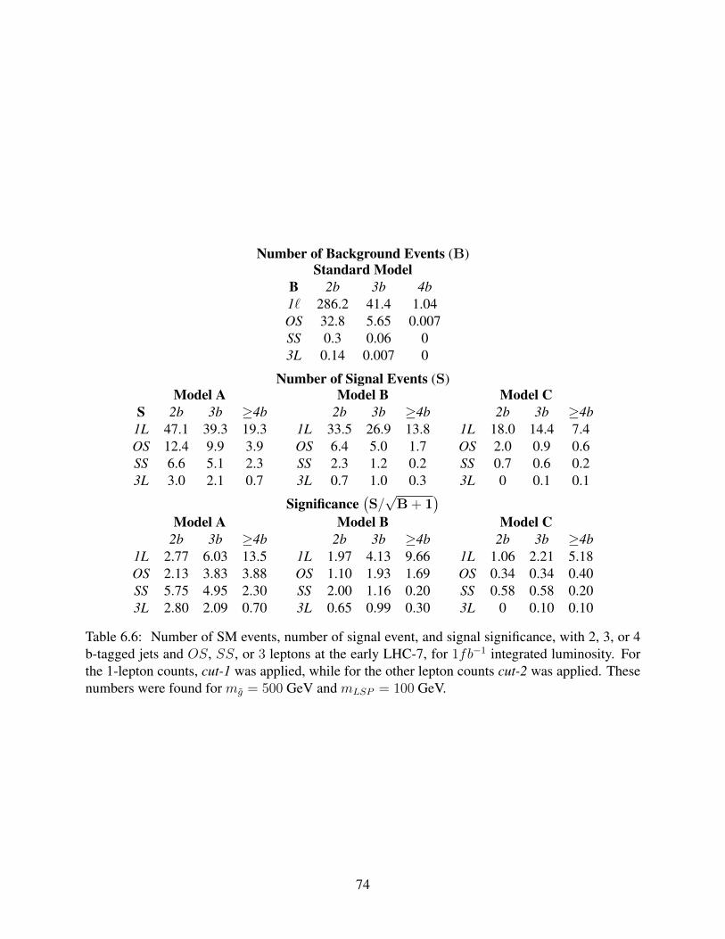
Number of Background Events (B)Standard Model

B 2b 3b 4b1` 286.2 41.4 1.04OS 32.8 5.65 0.007SS 0.3 0.06 03L 0.14 0.007 0

Number of Signal Events (S)Model A Model B Model C

S 2b 3b ≥4b1L 47.1 39.3 19.3OS 12.4 9.9 3.9SS 6.6 5.1 2.33L 3.0 2.1 0.7

2b 3b ≥4b1L 33.5 26.9 13.8OS 6.4 5.0 1.7SS 2.3 1.2 0.23L 0.7 1.0 0.3

2b 3b ≥4b1L 18.0 14.4 7.4OS 2.0 0.9 0.6SS 0.7 0.6 0.23L 0 0.1 0.1

Significance(S/√B + 1

)Model A Model B Model C

2b 3b ≥4b1L 2.77 6.03 13.5OS 2.13 3.83 3.88SS 5.75 4.95 2.303L 2.80 2.09 0.70

2b 3b ≥4b1L 1.97 4.13 9.66OS 1.10 1.93 1.69SS 2.00 1.16 0.203L 0.65 0.99 0.30

2b 3b ≥4b1L 1.06 2.21 5.18OS 0.34 0.34 0.40SS 0.58 0.58 0.203L 0 0.10 0.10

Table 6.6: Number of SM events, number of signal event, and signal significance, with 2, 3, or 4b-tagged jets and OS, SS, or 3 leptons at the early LHC-7, for 1fb−1 integrated luminosity. Forthe 1-lepton counts, cut-1 was applied, while for the other lepton counts cut-2 was applied. Thesenumbers were found for mg = 500 GeV and mLSP = 100 GeV.

74

where θc is the Cabbibo and angle and the pion decay width fπ ∼ 130 MeV. For large valuesof µ & 1 TeV and moderate values of tan β the loop contribution dominates the mass splitting,resulting in a charged Wino lifetime cτ ∼ O(5) cm [171]2.

A prolific source of detectable charged Wino tracks results from three body decays of pairproduced gluinos, pp→ gg → W±, W 0+ jets. In typical heavy squark and Wino LSP models, thegluino has a O(50%) branching ratio to W± final states; these events result in many hard objects,and are easily triggered on [179, 180]. The NLO gluino pair production cross section for the massrange of interest, 600 GeV . mg . 1000 GeV, is O(10 − 1000) fb. Increasing the LHC centerof mass energy from

√s = 7 TeV to

√s = 8 TeV approximately doubles the gluino production

cross section (as calculated by PROSPINO[181]). Thus with 10 fb−1 of luminosity, we shouldalready expect numerous gluino pair production events at LHC-8; roughly half of these gluinoswill produce a charged Wino as a 3-body decay product, since the SU(2) symmetry relates thebranching ratio to qqW 0, q′qW− and q′qW+.

In order to detect charged Winos resulting from gluino decays, W± must live long enough toform a track in the inner detector. Specifically, we focus on the detection capabilities of the AT-LAS detector. In the barrel region, the inner detector of the ATLAS detector contains three layersof pixel detector at average radii of 5 cm, 9 cm, 12 cm, then there are four layers of semiconductortracker (SCT), located respectively at 30 cm, 37 cm, 44 cm and 51 cm away from the beam line.The transition radiation tracker (TRT) is located outside the SCT, 55.4 cm away from the beamline [182]. If the charged Wino reaches the third layer of the SCT its track can be reconstructedusing the information from the pixel detector and the SCT, and its three-momentum can be de-termined with good resolution [183]. Perhaps it will be possible to use shorter chargino tracks.The soft pion (or lepton) resulting from the chargino decay would also be a distinctive signal if itcould be observed, and would give useful information regarding the kinematics of the event. To

mW 1st SCT Layer 2nd SCT Layer 3rd SCT Layer 4th SCT Layer100 GeV 416.3 292.6 208.2 147.9150 GeV 232.2 150.6 98.9 69.5200 GeV 125.3 76.5 46.4 30.8250 GeV 85.2 42.2 24.7 14.8300 GeV 49.7 27.6 17.0 9.4

Table 6.7: Inclusive count of the number of charginos which make it past a given detector layer.These results correspond to 10 fb−1 of LHC-8 data (σgg ∼ 235 fb), with mg = 750 GeV.

estimate the usefulness of looking for stiff charginos, we simulate decays of charged Winos result-ing from gluino pair production. The pair produced gluino events are generated by the MadGraph

2However if µ ∼ M2, there is an O(mW2/µ2) tree level mass splitting which can potentially become O(1) GeV,

significantly decreasing the lifetime such that cτ � 1 cm.

75

0.3 0.4 0.5 0.6 0.7 0.8 0.9 1.00

20

40

60

80

100

Transverse Distance Traveled HmL

Num

ber

ofC

harg

inos

�10

cm�

LH

C-

8,10

fb-

1

Figure 6.3: Charged Winos resulting from gluino pair production, binned as a function of trans-verse distance traveled from the beam line. These results correspond to 10 fb−1 of LHC-8 data(σgg ∼ 235 fb), with mg = 750 GeV, mW = 150 GeV. For graphical purposes, charginos travelinga transverse distance < 30 cm are not shown.

5/MadEvent package [184], and the gluino decays (as well as hadronization and showering) areimplemented through PYTHIA6 [153]. The mass splitting δm which enters into the decay widthis calculated using SOFTSUSY [185]. The results for mg = 750 GeV3 with 10 fb−1 of LHC-8data (without any kinematic cuts) are shown in Figure 1 and Table 1. In Fig. 1, the charged Winos4

are binned as a function of transverse distance traveled before decay. Table 1 shows an inclusivecount of the number charginos which make it past a given detector layer. These results indicatethat with the 10 fb−1 of LHC-8 data expected at the end of 2012, for mW . 300 GeV we expect& 20 charginos will make it past the third SCT layer.

To search for gluinos, one can use the usual SUSY search channels (or even looser cuts) toisolate relatively pure events from the gluino decay, and then search for chargino tracks in thoseevents. For a concrete example, in the G2-MSSM (resulting from M-theory compactified on aG2 manifold [187]) the gluino has a substantial branching fraction to third generation quarks:g → tbW− + h.c.. As demonstrated in [179, 180], searching for events containing a lepton andmultiple b-jets is the most powerful way to discover this kind of model. With the additional signalsgiven by chargino tracks, one can also make use of the weaker SUSY search channels such as 1

3We note that with heavy squarks, and the enhancement of gluino decays to heavy quarks due to a lighter stop andsbottom, 750 GeV gluinos are not excluded by any ATLAS or CMS analysis.

4In order for the non-thermal cosmology to give approximately correct relic density and not overclose the universe,the chargino cannot be very heavy, so we only consider charginos mass from 100 GeV to 300 GeV[186].

76

lepton + 1 b-jet. As an example, we consider a G2-MSSM model with a 750 GeV gluino and 150GeV Wino LSP with 10 fb−1 of LHC-8 data5. After applying cuts similar to the 1 lepton + 1 b-jetATLAS search channel[188]:

1 lepton, 6ET > 80 GeV, ≥ 4 jets, ≥ 1 b-jets, (6.4)

about 200 gluino pair events survive. Roughly 10 of these surviving events will contain a longchargino track which can be reconstructed. Aside from the 1 lepton + 1 b-jet channel, this charginosignal can be observed in many other SUSY channels, as illustrated in Table 2. In this table, thekinematic cuts defining the signal regions of the 1 b-jet + 6ET channel are defined in [188], andthe cuts defining the signal regions of the jets + 6ET channel are defined in [189]. These results

b-jets + 6ET Signal Region[188] SR0-A1meff >500

SR0-B1meff >700

SR0-C1meff >900

Charginos Past 3rd SCT 28 25 17jets + 6ET Signal Region[189] 4-jet,

meff >5004-jet,meff >1000

4-jet,High Mass

Charginos Past 3rd SCT 40 26 20

Table 6.8: Number of charginos which make it past the 3rd SCT layer in signal regions of variousATLAS SUSY search channels. These results are for 10 fb−1 of LHC-8 data. We have chosenchannels expected to be sensitive to gluino pair production events. Other search channels giveweaker chargino signals, which can be enhanced by loosening cuts. The meff cuts are given inunits of GeV.

demonstrate that the signal of chargino tracks is robust under typical SUSY squark/gluino searchcuts; in particular, increasing themeff cut from 500 GeV to 1000 GeV still maintains∼ 60% of thechargino signal. Thus chargino tracks provide an additional “free” channel for gluino discovery,which can be studied without loosening cuts and introducing additional SM background eventsinto the SUSY signal region.

The stub track resulting from chargino decay is a distinctive SUSY signal without SM back-ground. However, in reality the signal may be contaminated by detector noise and mis-reconstructedtracks. We did not include these possible backgrounds in our study; instead we argue they can becontrolled without significantly hurting the signals. First of all, the kinematic cuts we applied toremove a large amount of the SM background should also help reduce fake chargino tracks. Re-quiring pT > 80 GeV for the chargino track candidate keeps ∼ 80% of the signal events, whileeliminating detector noise resulting from soft mis-reconstructed tracks. For a fake track with high

5Detector effects are included by running simulated events through the PGS-4[154] detector simulation.

77

pT , the fake chargino pT will be nearly collinear with 6ET unless there are large contributions to 6ETfrom energetic neutrinos. Thus imposing a ∆φ (W±, 6ET ) > 0.4 cut will reduce the backgroundfrom hard jets faking chargino tracks, while keeping ∼ 60% of the signal events. In addition,the pixel detector can measure dE/dx energy loss of the particle. The charginos on average haveβγ = 2, while the SM tracks with the same momentum have much larger βγ. It is possible that thisenergy loss can be used to separate the real chargino tracks from the backgrounds. With enoughevents, dE/dx spectra can even be used to estimate the mass of the chargino. However, precisedetermination of the background after imposing cuts can only be determined by experimental de-tector groups upon analyzing the data.

6.5 Reconstructing the Gluino Mass

If chargino tracks are observed, one can use this additional information to separate SUSY eventsfrom the SM background, and estimate the mass of the gluino even without precise knowledge ofthe chargino mass. As already mentioned in the ATLAS jets + 6ET search, ignoring the chargino/LSPmass only changes the reconstructed gluino mass by a small amount, O(m2

LSP/m2g). To obtain suf-

ficient statistics for the analysis, we use a set of cuts slightly looser than the cuts used in the ATLASjets + 6ET search[189]:

6ET > 130 GeV, ≥ 4 jets, pT (j1) > 130 GeV,

pT (j2, j3, j4) > 50 GeV, ∆R(chargino, jets) > 0.3 (6.5)

For 10 fb−1 of LHC-8 data, there will be about 60 events containing a reconstructed charginotrack which pass the cuts listed in (??). In order to find the pair of jets most likely to havecome from the same gluino as the chargino track, we calculate the transverse momentum of theother chargino/neutralino from the missing transverse momentum, and separate the 6 objects (2charginos and 4 jets) into 2 clusters, each containing 1 chargino and 2 jets. The optimal clusteringis determined by minimizing the difference in |pT | between the two clusters. Using the clustercontaining the real chargino track and assuming mW = 0, we can make a histogram of the re-constructed gluino mass. Fitting the histogram with a distribution gives a reconstructed gluinomass near the actual value, with ∼ 100 GeV uncertainty. Thus chargino tracks can provide anindependent kinematic measure of the gluino mass, whose accuracy will improve with improvingstatistics.

Simply knowing that a gluino of some approximately measured mass decays to a chargino +jets of some pT puts a valuable upper limit on the chargino mass (and therefore the dark mattermass). With more information, it may be possible to obtain a precise measurement of the chargino

78

mass. For instance, measuring the pT of the soft pion resulting from the chargino decay alongwith the chargino track 3-momentum might allow a kinematic reconstruction of the chargino mass.However, it is unclear whether or not measuring such a soft track would be experimentally feasible.Other experimental approaches, such as determining the dE/dx spectra of the chargino tracks, canalso refine measurements of the chargino mass.

Since these analysis were done, the LHC detector groups have presented gluino searches thatexcluded the light gluino masses. Since none of the analysis use the realistic gluion branchingratio such as BR(tt) ≈ 7%, BR(bb) ≈ 10%, BR(tb + tb) ≈ 26%, it is not easy to use the reportedresults to give precise gluino limits; we estimate that mg < 950 GeV is probably excluded, butTeV gluinos are not.

79

CHAPTER 7

Conclusion

7.1 conclusion and future directions

In this thesis I studied G2 compactification of the M theory. The moduli stabilization and SUSYbreaking are achieved by hidden sector QCD like interactions. To obtain a de Sitter space witha small cosmological constant, a meson field from the quark condensation has to be included.Motivated by our knowledge about the Calabi-Yau manifold, it is plausible to have a G2 manifoldwith a discrete symmetry after moduli stabilization.

Once we establish all the theoretical ingredients, we focused on the SU(5) GUT model. Wilsonlines are introduced to break the SU(5) to the standard model gauge group SU(3)×SU(2)×U(1).By combining them with appropriate discrete symmetries on the G2 manifold, we can solve thedoublet-triplet splitting problem. The effective theory below the unification scale, G2-MSSM, hasa MSSM spectrum with distinctive features such as heavy scalars, suppressed µ term and lightgauginos. The matter/R-parity can be realized as another discrete symmetry on the stabilized G2

manifold. Anomaly-free conditions put non-trivial constrains not only on the discrete symmetryitself, but also on the Yukawa couplings. The approximate symmetry suppressing the µ term willalso suppress at least one eigenvalue of the Yukawa matrix of the down-type quarks or the leptons.Then we demonstrated the little hierarchy problem is alleviated in the G2-MSSM because of thelarge trilinear couplings. The compactification predicts the gravitino mass is exponentially sup-pressed comparing to the Planck scale. The lower bound of the moduli/gravitino mass is obtainedfrom cosmology. To preserve the well established BBN mechanism, it is important that the moduliand the gravitino decay well before BBN time. This in turn requires m3/2 ∼ O(50 TeV).

The rest of this thesis focused on the phenomenology of G2-MSSM. First we considered thedark matter candidates. Wino LSP and axion are both good candidates for dark matter and therelic abundances of both are of the same order according to the theoretical calculation. Wino LSPhas a large annihilation cross section. It can be used to partially explain the “anomalies” in theobservation of recent indirect dark matter experiments. The direct detection experiments are more

80

challenging for wino dark matter due to its very small cross section. The only way to increase thecross section is to increase the Higgsino component by lowering the µ term. However the µ termis determined from the top-down approach independently. Thus we can obtain a upper limit of thedirect detection cross section well below the current experimental bounds.

The LHC phenomenology had two parts. First we calculated the Higgs mass in G2-MSSM.Because of the heavy scalars, the lightest Higgs particle received large loop corrections. Afterresuming the major contributions, the mass of the lightest Higgs particle in G2-MSSM is close to125 GeV, about ±1.5 GeV for tan β prefered by the theory, which is consistent with the recentresults from ATLAS [10] and CMS [11]. The more exciting possibility is the direct observation ofsuperparticles at the LHC. Because the scalars are too heavy to be produced directly, we concen-trated on the light gauginos. Gluino searches using MET and multijets are always a good approach.In some cases the decay branching fractions to the 3rd generation quarks are enhanced, so target-ing channels with b-jets and/or leptons with large MET can be more effective. There is also apotentially interesting search channel for the light chargino. The disappearing chargino tracks arenot only useful in searching for new physics, but can also provide extra kinematic information forquantitative studies.

On the theoretical aspect, G2-manifolds are notoriously difficult to construct, but new develop-ments in recent years might soon evolve to produce compactG2-manifolds with singularities suitedfor phenomenological purposes. It is also important to understand the top Yukawa coupling in Mtheory. There is a construction for the standard model gauge group, but there is still no satisfyingsolution for unification theories.

We will understand the phenomenology a lot better with deeper knowledge of theG2-manifold.Meanwhile it is interesting to consider the phenomenology of more general scenarios like enlargedgauge group such as SO(10), or extra matter fields.

81

APPENDIX A

Useful Results

A.1 Implications of Top-Down Constraints

A.1.1 Constraints on Wilson Line Parameters from Anomaly Cancellation

The SU(3)−SU(3)−ZN , SU(2)−SU(2)−ZN and U(1)Y −U(1)Y −ZN anomaly coefficientsfor a non-R ZN symmetry are given by:

ASU(3)−SU(3)−ZN ≡ A3 =1

2

3∑i=1

(2qQi + qU i + qDi

)+

1

2(qTu + qTd)

ASU(2)−SU(2)−ZN ≡ A2 =1

2

3∑i=1

(3qQi + qLi

)+

1

2(qHu + qHd)

AU(1)−U(1)−ZN ≡ A1 =1

2

3∑i=1

(1

5qQi +

8

5qU i +

6

5qEic +

2

5qDi +

3

5qLi

)+

1

5(qTu + qTd) +

3

10(qHu + qHd) (A.1)

where qQi represents the ZN charge for the i’th generation of theQ superfield, and similarly forqU i , qDi , etc. As discussed in section 3.2.5.1, anomaly cancellation requires that 3.25 is satisfied.Furthermore, consitency with the Wilson line mechanism described in Chapter 3 requires that (3.4)-(3.6) are satisfied. It is straightforward to show using (3.4) and (3.5) that the anomaly coefficientsin (A.1) satisfy:

2A3 + 3A2 = 5A1. (A.2)

Therefore A1 provides no additional constraint, and anomaly cancellation is achieved providedthe conditions on A3 and A2 in (3.25) are satisfied. In other words, A3 = A2 is sufficient to

82

achieve anomaly cancellation regardless of whether or not a Green-Schwarz axion is present. Bycombining the condition A3 = A2 with (3.4)-(3.6), we obtain:

3∑i=1

5ρ(δ5i− δ10i

)= 5ρ

(δ5H − δ5H

)Mod N = qHu + qHd . (A.3)

Here the δ10i and δ5 parameterize the Wilson line splitting of the SU(5) multiplets, and thesum over i represents a sum over all three generations. Since doublet-triplet splitting requires5ρ 6= Mod N and recalling that by our parameterization δi = 0 or 1, we can enumerate thepossible solutions to (3.25):

1.∑3

i=1

(δ5i− δ10i

)=(δ5H − δ5H

). In this case, the anomaly constraints are trivially satisfied

regardless of the value which 5ρ takes.

2.∑3

i=1

(δ5i− δ10i

)= −

(δ5H − δ5H

)or∑3

i=1

(δ5i− δ10i

)= 3

(δ5H − δ5H

). In this case, the

anomaly constraints are satisfied if 10ρ = N . This requires evenN and results in 5ρ = N/2,and thus ZM = ZN/2 assuming no other moduli charges.

3.∑3

i=1

(δ5i− δ10i

)= −2

(δ5H − δ5H

). In this case, anomaly freedom requires 15ρ = N , and

thus 5ρ = N/3.

4.∑3

i=1

(δ5i− δ10i

)= −3

(δ5H − δ5H

). In this case, anomaly freedom requires 20ρ = N, 2N

and thus 5ρ = N/2, N/4.

A.1.2 Fermion Mass Forbidden by ZN

For the ZN solution to the µ problem described in this work, top-down constraints imply that atleast one of the mass eigenvalues in either the down or lepton sector must be forbidden by ZN ifZN solves the doublet-triplet splitting problem. In what follows, we give a simple derivation ofthis result.

A three by three matrix A with entries Ai,j will have a nonzero determinant if:

Π3i=1 (Ai,σi) 6= 0. (A.4)

where σi is some permutation of 1, 2 and 3. For example, if we are considering the diagonalcomponents of A then (σ1, σ2, σ3) = (1, 2, 3), and (A.4) would result in A11A22A33 6= 0. If A hasa zero diagonal component, detA 6= 0 if (A.4) is satisfied for some other permutation σi.

If all mass eigenvalues in the down quark sector are allowed by ZN , then (A.4) amounts to acondition on the ZN charges of MSSM fields:

83

qQi + qHd + qDcσ(i)

= 0, (A.5)

for i = 1, 2, 3. A similar equation with Li and Ecσ(i) arises from the lepton Yukawa matrix.

Regardless of the permutation chosen for σi, we can sum (A.5) over i and obtain the conditionsfor all lepton and down quark mass eigenvalues to be allowed by ZN :

3∑i=1

qQi + qHd + qDci = 03∑i=1

qLi + qHd + qEci = 0. (A.6)

Using (4) and (5) this can be rewritten as:

3∑i=1

5ρ(δ10i − δ5i

)= Mod N. (A.7)

From equation (A.7), we see that this can not be satisfied if ZN achieves doublet-triplet split-ting. Therefore if the ZN discussed here solves the µ problem, then at least one mass in thedown/lepton sector is forbidden by ZN and must be generated in some manner once ZN is broken.

A.1.3 Constraints on the LSP Lifetime

The constraints on the LSP lifetime can by approximated as [190]:

τLSP . 0.1 seconds or τLSP & 1025 seconds (A.8)

The bound τLSP . 0.1 second comes from primordial nucleosynthesis constraints on long-lived BSM [191, 192, 193, 194, 195], and the bound τLSP & 1025 seconds comes from indirectdetection constraints. In the case of purely trilinear RPV (i.e. no blinear RPV operator present),the LSP lifetime is given by:

τlsp1 sec

≈ 10−17

λ2

( m0

TeV

)4(

100 GeV

mLSP

)5

. (A.9)

where λ is the dominant trilinear RPV coupling in λ, λ′, λ′′ following the notation of (3.27).Taking the squark mass m0 to be 10 TeV and mLSP = 100 GeV, the constraint (A.8) can beexpressed as:

λ & 10−6 or λ . 10−19. (A.10)

As previously discussed, if moduli stablization regenerates the trilinear RPV coupling then λ ∼O (10−15). Therefore if the only form of RPV in the theory is a trilinear RPV term forbidden by

84

ZN but generated by moduli stablization, the theory will be ruled out by experimental constraintson LSP lifetime.

A.2 Largest Spin Independent Cross Sections

Following [110], the spin-independent cross section for the LSP scattering off a nucleon, is givenin the decoupling limit (MZ �MA) by the approximation

σSI (χN → χN) ≈ 5× 10−45cm2

(115 GeV

mh

)4(ZHu sin β − ZHd cos β

0.1

)2

(ZW − tan θWZB)2

(A.11)where the Z’s give the composition of the LSP

χ ≡ ZB B + ZW W + ZHd Hd + ZHu Hu. (A.12)

Consider the neutralino mass matrix [196]:

M =

M1 0 −MZ cos β sin θW MZ sin β sin θW

0 M2 MZ cos β cos θW −MZ sin β cos θW

−MZ cos β sin θW MZ cos β cos θW 0 −µMZ sin β sin θW −MZ sin β cos θW −µ 0

(A.13)

in the {B, W , Hd, Hu} basis.The analytical expression [111, 112, 113] for the components in theLSP can be written as:

αZB = zB = − sin θW

αZW = zW = cos θWM1 −Mχ

M2 −Mχ

= cos θW(M1 −Mχ)2

∆

αZHd = zHd =µ (M1 −Mχ) (M2 −Mχ) +M2

Z sin β cos β ((M1 −M2) cos2 θW +M2 −Mχ)

MZ (M2 −Mχ) (−µ cos β +Mχ sin β)

αZHu = zHu =Mχ (M1 −Mχ) (M2 −Mχ) +M2

Z cos2 β ((M1 −M2) cos2 θW +M2 −Mχ)

MZ (M2 −Mχ) (−µ cos β +Mχ sin β)

(A.14)

where α =√z2B + z2

W + z2Hd

+ z2Hu

is an overall normalization factor and ∆ ≡ (Mχ−M1)(Mχ−M2).

The combination ZHu sin β − ZHd cos β, that appears in the scattering cross section takes an

85

especially simple form

ZHu sin β − ZHd cos β =(Mχ sin β − µ cos β) (M1 −Mχ) (M2 −Mχ)

MZ (M2 −Mχ) (−µ cos β +Mχ sin β)=M1 −Mχ

MZ

. (A.15)

It is clear from (A.15) that as M1 −Mχ increases, ZHu sin β − ZHd cos β grows slower than theZW component. Thus after normalization both the Hu and the Hd components will decrease. Sothe maximum of ZHu sin β − ZHd cos β is realized when M1 −Mχ is minimal.

The eigenvalues of the neutralino mass matrix (A.13) are given by the solutions to:

(x−M1) (x−M2) (x− µ) (x+ µ) +(M1 cos2 θW +M2 sin2 θ

)M2

Zµ sin 2β = 0 (A.16)

Then the LSP mass, corresponding to Mχ ≡ x, can be found by taking the limit Mχ � µ,so that (A.16) is simply a quadratic equation. Then it is easy to see that the minimal value ofM1 −Mχ, which maximizes ZHu sin β − ZHd cos β, corresponds to the situation when M1 −M2

is also minimized. Additionally, when M1 = M2, the term ZW − tan θWZB also reaches itsmaximum. Thus the maximum scattering cross sections will occur when M1 = M2.

To normalize the expressions in (A.14) (i.e. finding α) is tedious. Instead, a new basis is definedwhere γ = cos θW B + sin θW W and Z = − sin θW B + cos θW W , where in the supersymmetriclimit, these are the superpartners of the photon and Z-boson, respectively. The new mass matrix,in the {γ, Z, Hd, Hu} is

M =

M1cos θW

2 +M2sin θW2 (M2 −M1) sin θW cos θW 0 0

(M2 −M1) sin θW cos θW M2cos θW2 +M1sin θW

2 MZ cos β −MZ sin β

0 MZ cos β 0 −µ0 −MZ sin β −µ 0

(A.17)

Taking the limit M1 = M2 ≡ M , one immediately one finds that γ in an eigenvector with masseigenvalue M . The next lightest eigenvector of the remaining 3 × 3 sub-matrix will be mostly Z,and to leading order in MZ/µ, the mass is

Mχ 'M − M2Z

µ

(M

MZ

− sin 2β

)(A.18)

Next we will assume that the phases of M and µ are such that absolute value of Mχ is smallerthan |M |, so that it is indeed the LSP. The other scenario, in which the LSP is mostly γ, will havenegligible scattering cross-section.

Diagonalizing the remaining 3 × 3 sub-matrix, the coefficients of Hu and Hd component to

86

leading order is

ZHd =1

2

((sin β − cos β)MZ

µ+M+

(sin β + cos β)MZ

µ−M

)=MZ (µ sin β +M cos β)

µ2 −M2

ZHu =1

2

((sin β − cos β)MZ

µ+M− (sin β + cos β)MZ

µ−M

)= −MZ (µ cos β +M sin β)

µ2 −M2(A.19)

and from the definition on Z,

ZW − tan θWZB = cos θW−1. (A.20)

Finally, using (A.19) and (A.20) as inputs to (A.11) the upper limit for the cross section is

σSI (χN → χN) ≈ 6× 10−45cm2

(115 GeV

mh

)4(1 TeV

µ

)2(sin 2β +M2/µ

1− (M2/µ)2

)2

(A.21)

From the discussion in the text we expect M2/µ . 0.2, sin 2β . 0.8 and µ & 1 TeV, givinglargest scattering cross-sections around σSI . 6 × 10−45cm2. However, as discussed in Section6.3, the constraints cannot all be satisfied simultaneously, so in practice only a cross section ofabout 10−45 cm2 could be achieved.

87

BIBLIOGRAPHY

[1] PAMELA Collaboration, O. Adriani et al., “An anomalous positron abundance in cosmicrays with energies 1.5.100 GeV,” Nature 458 (2009) 607–609, arXiv:0810.4995[astro-ph].

[2] AMS Collaboration Collaboration, M. Aguilar et al., “First Result from the AlphaMagnetic Spectrometer on the International Space Station: Precision Measurement of thePositron Fraction in Primary Cosmic Rays of 0.5350 GeV,” Phys.Rev.Lett. 110 no. 14,(2013) 141102.

[3] O. Adriani et al., “A new measurement of the antiproton-to-proton flux ratio up to 100GeV in the cosmic radiation,” Phys. Rev. Lett. 102 (2009) 051101, arXiv:0810.4994[astro-ph].

[4] J. J. Engelmann, P. Ferrando, A. Soutoul, P. Goret, and E. Juliusson, “Charge compositionand energy spectra of cosmic-ray nuclei for elements from Be to NI - Results fromHEAO-3-C2,” Astronomy and Astrophysics 233 (July, 1990) 96–111.

[5] The Fermi LAT Collaboration, A. A. Abdo et al., “Measurement of the Cosmic Ray e+plus e- spectrum from 20 GeV to 1 TeV with the Fermi Large Area Telescope,”arXiv:0905.0025 [astro-ph.HE].

[6] D. Feldman, Z. Liu, and P. Nath, “Gluino NLSP, Dark Matter via Gluino Coannihilation,and LHC Signatures,” Phys.Rev. D80 (2009) 015007, arXiv:0905.1148 [hep-ph].

[7] S.-T. Yau, “On the ricci curvature of a compact Kahler manifold and the complexMonge-Ampere equation, I,” Comm. Pure Appl. Math. 31 (1978) 339.

[8] B. S. Acharya, K. Bobkov, G. L. Kane, J. Shao, and P. Kumar, “The G2-MSSM - An MTheory motivated model of Particle Physics,” Phys. Rev. D78 (2008) 065038,arXiv:0801.0478 [hep-ph].

[9] B. S. Acharya and K. Bobkov, “Kahler Independence of the G(2)-MSSM,” JHEP 1009(2010) 001, arXiv:0810.3285 [hep-th].

[10] “Combined coupling measurements of the higgs-like boson with the atlas detector using upto 25 fb−1 of proton-proton collision data,” Tech. Rep. ATLAS-CONF-2013-034, CERN,Geneva, Mar, 2013.

88

[11] “Combination of standard model higgs boson searches and measurements of the propertiesof the new boson with a mass near 125 gev,” Tech. Rep. CMS-PAS-HIG-13-005, CERN,Geneva, 2013.

[12] D. Joyce, “Compact Riemannian 7-manifolds with holonomy G2. Part I,” J.Diff.Geom. 43(1996) 291.

[13] D. Joyce, “Compact Riemannian 7-manifolds with holonomy G2. Part II,” J.Diff.Geom. 43(1996) 329.

[14] M. Atiyah and E. Witten, “M theory dynamics on a manifold of G(2) holonomy,”Adv.Theor.Math.Phys. 6 (2003) 1–106, arXiv:hep-th/0107177 [hep-th].

[15] A. Corti, M. Haskins, J. Nordstrom, and T. Pacini, “G2-manifolds and associativesubmanifolds via semi-Fano 3-folds,” arXiv:1207.4470 [math.DG].

[16] B. S. Acharya, “On Realizing N=1 superYang-Mills in M theory,”arXiv:hep-th/0011089 [hep-th].

[17] B. S. Acharya, “M theory, Joyce orbifolds and superYang-Mills,” Adv.Theor.Math.Phys. 3(1999) 227–248, arXiv:hep-th/9812205 [hep-th].

[18] E. Witten, “Anomaly cancellation on G(2) manifolds,” arXiv:hep-th/0108165[hep-th].

[19] B. S. Acharya and E. Witten, “Chiral fermions from manifolds of G(2) holonomy,”arXiv:hep-th/0109152 [hep-th].

[20] B. S. Acharya and S. Gukov, “M theory and singularities of exceptional holonomymanifolds,” Phys.Rept. 392 (2004) 121–189, arXiv:hep-th/0409191 [hep-th].

[21] T. Friedmann and E. Witten, “Unification scale, proton decay, and manifolds of G(2)holonomy,” Adv.Theor.Math.Phys. 7 (2003) 577–617, arXiv:hep-th/0211269[hep-th].

[22] T. Pantev and M. Wijnholt, “Hitchin’s Equations and M-Theory Phenomenology,”J.Geom.Phys. 61 (2011) 1223–1247, arXiv:0905.1968 [hep-th].

[23] M. B. Green and J. H. Schwarz, “Anomaly Cancellation in Supersymmetric D=10 GaugeTheory and Superstring Theory,” Phys.Lett. B149 (1984) 117–122.

[24] S. M. Barr, “A New Symmetry Breaking Pattern for SO(10) and Proton Decay,” Phys.Lett.B112 (1982) 219.

[25] J. Derendinger, J. E. Kim, and D. V. Nanopoulos, “Anti-SU(5),” Phys.Lett. B139 (1984)170.

[26] I. Antoniadis, J. R. Ellis, J. Hagelin, and D. V. Nanopoulos, “Supersymmetric FlippedSU(5) Revitalized,” Phys.Lett. B194 (1987) 231.

89

[27] E. Kuflik and J. Marsano, “Comments on Flipped SU(5) (and F-theory),” JHEP 1103(2011) 020, arXiv:1009.2510 [hep-ph].

[28] B. S. Acharya, K. Bobkov, G. Kane, P. Kumar, and D. Vaman, “An M theory Solution tothe Hierarchy Problem,” Phys.Rev.Lett. 97 (2006) 191601, arXiv:hep-th/0606262[hep-th].

[29] B. S. Acharya, K. Bobkov, G. L. Kane, P. Kumar, and J. Shao, “Explaining the ElectroweakScale and Stabilizing Moduli in M Theory,” Phys.Rev. D76 (2007) 126010,arXiv:hep-th/0701034 [hep-th].

[30] B. S. Acharya, F. Denef, and R. Valandro, “Statistics of M theory vacua,” JHEP 0506(2005) 056, arXiv:hep-th/0502060 [hep-th].

[31] J. M. Maldacena and C. Nunez, “Supergravity description of field theories on curvedmanifolds and a no go theorem,” Int.J.Mod.Phys. A16 (2001) 822–855,arXiv:hep-th/0007018 [hep-th].

[32] B. S. Acharya, G. Kane, and E. Kuflik, “String Theories with Moduli Stabilization ImplyNon-Thermal Cosmological History, and Particular Dark Matter,” arXiv:1006.3272[hep-ph].

[33] E. Witten, “Deconstruction, G(2) holonomy, and doublet triplet splitting,”arXiv:hep-ph/0201018 [hep-ph].

[34] A. Brignole, L. E. Ibanez, and C. Munoz, “Soft supersymmetry breaking terms fromsupergravity and superstring models,” arXiv:hep-ph/9707209 [hep-ph].

[35] B. S. Acharya et al., “Non-thermal Dark Matter and the Moduli Problem in StringFrameworks,” JHEP 06 (2008) 064, arXiv:0804.0863 [hep-ph].

[36] Y. Kawamura, “Triplet doublet splitting, proton stability and extra dimension,”Prog.Theor.Phys. 105 (2001) 999–1006, arXiv:hep-ph/0012125 [hep-ph].

[37] L. J. Hall and Y. Nomura, “Gauge unification in higher dimensions,” Phys.Rev. D64 (2001)055003, arXiv:hep-ph/0103125 [hep-ph].

[38] L. J. Hall, H. Murayama, and Y. Nomura, “Wilson lines and symmetry breaking onorbifolds,” Nucl.Phys. B645 (2002) 85–104, arXiv:hep-th/0107245 [hep-th].

[39] Y. Kawamura and T. Miura, “Classification of Standard Model Particles in E6 OrbifoldGrand Unified Theories,” arXiv:1301.7469 [hep-ph].

[40] E. Witten, “Deconstruction, G(2) holonomy, and doublet triplet splitting,”arXiv:hep-ph/0201018 [hep-ph].

[41] L. M. Krauss and F. Wilczek, “Discrete Gauge Symmetry in Continuum Theories,”Phys.Rev.Lett. 62 (1989) 1221.

90

[42] Y. Hosotani, “Dynamical Mass Generation by Compact Extra Dimensions,” Phys.Lett.B126 (1983) 309.

[43] P. Candelas, G. T. Horowitz, A. Strominger, and E. Witten, “Vacuum Configurations forSuperstrings,” Nucl.Phys. B258 (1985) 46–74.

[44] G. Giudice and A. Masiero, “A Natural Solution to the mu Problem in SupergravityTheories,” Phys.Lett. B206 (1988) 480–484.

[45] J. Wess and J. Bagger, “Supersymmetry and supergravity,”.

[46] B. S. Acharya and M. Torabian, “Supersymmetry Breaking, Moduli Stabilization andHidden U(1) Breaking in M-Theory,” Phys.Rev. D83 (2011) 126001,arXiv:1101.0108 [hep-th].

[47] K. Babu, I. Gogoladze, and K. Wang, “Natural R parity, mu term, and fermion masshierarchy from discrete gauge symmetries,” Nucl.Phys. B660 (2003) 322–342,arXiv:hep-ph/0212245 [hep-ph].

[48] T. Araki, T. Kobayashi, J. Kubo, S. Ramos-Sanchez, M. Ratz, et al., “(Non-)Abeliandiscrete anomalies,” Nucl.Phys. B805 (2008) 124–147, arXiv:0805.0207[hep-th].

[49] M. Cvetic, I. Garcia Etxebarria, and J. Halverson, “Three Looks at Instantons in F-theory –New Insights from Anomaly Inflow, String Junctions and Heterotic Duality,” JHEP 1111(2011) 101, arXiv:1107.2388 [hep-th].

[50] H. M. Lee, S. Raby, M. Ratz, G. G. Ross, R. Schieren, et al., “Discrete R symmetries forthe MSSM and its singlet extensions,” Nucl.Phys. B850 (2011) 1–30,arXiv:1102.3595 [hep-ph].

[51] L. E. Ibanez and G. G. Ross, “Discrete gauge symmetries and the origin of baryon andlepton number conservation in supersymmetric versions of the standard model,” Nucl.Phys.B368 (1992) 3–37.

[52] L. E. Ibanez and G. G. Ross, “Discrete gauge symmetry anomalies,” Phys.Lett. B260(1991) 291–295.

[53] J. Preskill, S. P. Trivedi, F. Wilczek, and M. B. Wise, “Cosmology and broken discretesymmetry,” Nucl.Phys. B363 (1991) 207–220.

[54] T. Banks and M. Dine, “Note on discrete gauge anomalies,” Phys.Rev. D45 (1992)1424–1427, arXiv:hep-th/9109045 [hep-th].

[55] C. Csaki and H. Murayama, “Discrete anomaly matching,” Nucl.Phys. B515 (1998)114–162, arXiv:hep-th/9710105 [hep-th].

[56] H. M. Lee, S. Raby, M. Ratz, G. G. Ross, R. Schieren, et al., “Discrete R symmetries forthe MSSM and its singlet extensions,” Nucl.Phys. B850 (2011) 1–30,arXiv:1102.3595 [hep-ph].

91

[57] H. K. Dreiner, C. Luhn, and M. Thormeier, “What is the discrete gauge symmetry of theMSSM?,” Phys.Rev. D73 (2006) 075007, arXiv:hep-ph/0512163 [hep-ph].

[58] K. Kurosawa, N. Maru, and T. Yanagida, “Nonanomalous R symmetry in supersymmetricunified theories of quarks and leptons,” Phys.Lett. B512 (2001) 203–210,arXiv:hep-ph/0105136 [hep-ph].

[59] H. M. Lee, S. Raby, M. Ratz, G. G. Ross, R. Schieren, et al., “A unique ZR4 symmetry for

the MSSM,” Phys.Lett. B694 (2011) 491–495, arXiv:1009.0905 [hep-ph].

[60] J. L. Evans, M. Ibe, J. Kehayias, and T. T. Yanagida, “Non-Anomalous DiscreteR-symmetry Decrees Three Generations,” Phys.Rev.Lett. 109 (2012) 181801,arXiv:1111.2481 [hep-ph].

[61] M. Asano, T. Moroi, R. Sato, and T. T. Yanagida, “Non-anomalous Discrete R-symmetry,Extra Matters, and Enhancement of the Lightest SUSY Higgs Mass,” Phys.Lett. B705(2011) 337–341, arXiv:1108.2402 [hep-ph].

[62] M. Paraskevas and K. Tamvakis, “On Discrete R-Symmetries in MSSM and itsExtensions,” Phys.Rev. D86 (2012) 015009, arXiv:1205.1391 [hep-ph].

[63] R. Kappl, B. Petersen, S. Raby, M. Ratz, R. Schieren, et al., “String-Derived MSSM Vacuawith Residual R Symmetries,” Nucl.Phys. B847 (2011) 325–349, arXiv:1012.4574[hep-th].

[64] B. S. Acharya, G. Kane, E. Kuflik, and R. Lu, “Theory and Phenomenology of µ in Mtheory,” JHEP 1105 (2011) 033, arXiv:1102.0556 [hep-ph].

[65] H. Murayama and A. Pierce, “Not even decoupling can save minimal supersymmetricSU(5),” Phys.Rev. D65 (2002) 055009, arXiv:hep-ph/0108104 [hep-ph].

[66] I. Affleck and M. Dine, “A New Mechanism for Baryogenesis,” Nucl.Phys. B249 (1985)361.

[67] M. Ambroso and B. A. Ovrut, “The Mass Spectra, Hierarchy and Cosmology of B-LMSSM Heterotic Compactifications,” Int.J.Mod.Phys. A26 (2011) 1569–1627,arXiv:1005.5392 [hep-th].

[68] P. Langacker and J. Wang, “U(1)-prime symmetry breaking in supersymmetric E(6)models,” Phys.Rev. D58 (1998) 115010, arXiv:hep-ph/9804428 [hep-ph].

[69] M. Cvetic, J. Halverson, and R. Richter, “Mass Hierarchies versus proton Decay in MSSMOrientifold Compactifications,” arXiv:0910.2239 [hep-th].

[70] D. M. Pierce, J. A. Bagger, K. T. Matchev, and R.-j. Zhang, “Precision corrections in theminimal supersymmetric standard model,” Nucl.Phys. B491 (1997) 3–67,arXiv:hep-ph/9606211 [hep-ph].

92

[71] C. Csaki, A. Falkowski, Y. Nomura, and T. Volansky, “New Approach to the mu-BmuProblem of Gauge-Mediated Supersymmetry Breaking,” Phys.Rev.Lett. 102 (2009)111801, arXiv:0809.4492 [hep-ph].

[72] M. Dine, “Some issues in gauge mediation,” Nucl.Phys.Proc.Suppl. 62 (1998) 276–280,arXiv:hep-ph/9707413 [hep-ph].

[73] S. P. Martin and M. T. Vaughn, “Two loop renormalization group equations for softsupersymmetry breaking couplings,” Phys.Rev. D50 (1994) 2282,arXiv:hep-ph/9311340 [hep-ph].

[74] B. Allanach, “SOFTSUSY: a program for calculating supersymmetric spectra,”Comput.Phys.Commun. 143 (2002) 305–331, arXiv:hep-ph/0104145 [hep-ph].

[75] G. Degrassi, P. Slavich, and F. Zwirner, “On the neutral Higgs boson masses in the MSSMfor arbitrary stop mixing,” Nucl.Phys. B611 (2001) 403–422,arXiv:hep-ph/0105096 [hep-ph].

[76] A. Dedes and P. Slavich, “Two loop corrections to radiative electroweak symmetrybreaking in the MSSM,” Nucl.Phys. B657 (2003) 333–354, arXiv:hep-ph/0212132[hep-ph].

[77] P. Nath and R. L. Arnowitt, “Nonuniversal soft SUSY breaking and dark matter,” Phys.Rev.D56 (1997) 2820–2832, arXiv:hep-ph/9701301 [hep-ph].

[78] K. L. Chan, U. Chattopadhyay, and P. Nath, “Naturalness, weak scale supersymmetry andthe prospect for the observation of supersymmetry at the Tevatron and at the CERN LHC,”Phys.Rev. D58 (1998) 096004, arXiv:hep-ph/9710473 [hep-ph].

[79] J. L. Feng, K. T. Matchev, and T. Moroi, “Focus points and naturalness in supersymmetry,”Phys.Rev. D61 (2000) 075005, arXiv:hep-ph/9909334 [hep-ph].

[80] T. Banks, D. B. Kaplan, and A. E. Nelson, “Cosmological implications of dynamicalsupersymmetry breaking,” Phys.Rev. D49 (1994) 779–787, arXiv:hep-ph/9308292[hep-ph].

[81] B. de Carlos, J. Casas, F. Quevedo, and E. Roulet, “Model independent properties andcosmological implications of the dilaton and moduli sectors of 4-d strings,” Phys.Lett.B318 (1993) 447–456, arXiv:hep-ph/9308325 [hep-ph].

[82] M. Berg, D. Marsh, L. McAllister, and E. Pajer, “Sequestering in StringCompactifications,” JHEP 1106 (2011) 134, arXiv:1012.1858 [hep-th].

[83] B. S. Acharya, P. Grajek, G. L. Kane, E. Kuflik, K. Suruliz, et al., “Identifying Multi-TopEvents from Gluino Decay at the LHC,” arXiv:0901.3367 [hep-ph].

[84] L. Randall and R. Sundrum, “Out of this world supersymmetry breaking,” Nucl. Phys.B557 (1999) 79–118, arXiv:hep-th/9810155.

93

[85] P. Langacker, G. Paz, L.-T. Wang, and I. Yavin, “Z’-mediated Supersymmetry Breaking,”Phys. Rev. Lett. 100 (2008) 041802, arXiv:0710.1632 [hep-ph].

[86] T. Moroi and L. Randall, “Wino cold dark matter from anomaly-mediated SUSYbreaking,” Nucl. Phys. B570 (2000) 455–472, arXiv:hep-ph/9906527.

[87] G. Kane and S. Watson, “Dark Matter and LHC: What is the Connection?,” Mod. Phys.Lett. A23 (2008) 2103–2123, arXiv:0807.2244 [hep-ph].

[88] B. S. Acharya, K. Bobkov, and P. Kumar, “An M Theory Solution to the Strong CPProblem and Constraints on the Axiverse,” JHEP 1011 (2010) 105, arXiv:1004.5138[hep-th].

[89] K. Bobkov, V. Braun, P. Kumar, and S. Raby, “Stabilizing All Kahler Moduli in Type IIBOrientifolds,” JHEP 1012 (2010) 056, arXiv:1003.1982 [hep-th].

[90] M. Kamionkowski and M. S. Turner, “Thermal relics: Do we know their abundances?,”Phys. Rev. D42 (1990) 3310–3320.

[91] D. J. H. Chung, E. W. Kolb, and A. Riotto, “Nonthermal supermassive dark matter,” Phys.Rev. Lett. 81 (1998) 4048–4051, arXiv:hep-ph/9805473.

[92] G. F. Giudice, E. W. Kolb, and A. Riotto, “Largest temperature of the radiation era and itscosmological implications,” Phys. Rev. D64 (2001) 023508, arXiv:hep-ph/0005123.

[93] A. W. Strong and I. V. Moskalenko, “Propagation of cosmic-ray nucleons in the Galaxy,”Astrophys. J. 509 (1998) 212–228, arXiv:astro-ph/9807150.

[94] P. Gondolo, J. Edsjo, P. Ullio, L. Bergstrom, M. Schelke, and E. A. Baltz, “DarkSUSY:Computing supersymmetric dark matter properties numerically,” JCAP 0407 (2004) 008,arXiv:astro-ph/0406204.

[95] P. Gondolo, J. Edsjo, P. Ullio, L. Bergstrom, M. Schelke, E. A. Baltz, T. Bringmann, andG. Duda. http://www.physto.se/˜edsjo/darksusy.

[96] F. Donato, N. Fornengo, D. Maurin, and P. Salati, “Antiprotons in cosmic rays fromneutralino annihilation,” Phys. Rev. D69 (2004) 063501, arXiv:astro-ph/0306207.

[97] L. Bergstrom, J. Edsjo, M. Gustafsson, and P. Salati, “Is the dark matter interpretation ofthe EGRET gamma excess compatible with antiproton measurements?,” JCAP 0605(2006) 006, arXiv:astro-ph/0602632.

[98] BESS Collaboration, S. Orito et al., “Precision measurement of cosmic-ray antiprotonspectrum,” Phys. Rev. Lett. 84 (2000) 1078–1081, arXiv:astro-ph/9906426.

[99] BESS Collaboration, T. Maeno et al., “Successive measurements of cosmic-ray antiprotonspectrum in a positive phase of the solar cycle,” Astropart. Phys. 16 (2001) 121–128,arXiv:astro-ph/0010381.

94

[100] Y. Asaoka et al., “Measurements of cosmic-ray low-energy antiproton and proton spectrain a transient period of the solar field reversal,” Phys. Rev. Lett. 88 (2002) 051101,arXiv:astro-ph/0109007.

[101] J. Lavalle, J. Pochon, P. Salati, and R. Taillet, “Clumpiness of dark matter and positronannihilation signal: Computing the odds of the galactic lottery,”arXiv:astro-ph/0603796.

[102] J. Lavalle, Q. Yuan, D. Maurin, and X. J. Bi, “Full Calculation of Clumpiness Boost factorsfor Antimatter Cosmic Rays in the light of ΛCDM N-body simulation results,”arXiv:0709.3634 [astro-ph].

[103] J. M. Clem, D. P. Clements, J. Esposito, P. Evenson, D. Huber, J. L’Heureux, P. Meyer, andC. Constantin, “Solar Modulation of Cosmic Electrons,” Astrophysical Journal 464 (June,1996) 507–+.

[104] L. J. Gleeson and W. I. Axford, “Cosmic Rays in the Interplanetary Medium,”Astrophysical Journal 149 (Sept., 1967) L115–L118.

[105] L. Zhang and K. S. Cheng, “Cosmic-ray positrons from mature gamma-ray pulsars,”Astronomy and Astrophysics 368 (Mar., 2001) 1063–1070.

[106] S. Profumo, “Dissecting Pamela (and ATIC) with Occam’s Razor: existing, well-knownPulsars naturally account for the ’anomalous’ Cosmic-Ray Electron and Positron Data,”arXiv:0812.4457 [astro-ph].

[107] J. Diemand, B. Moore, and J. Stadel, “Earth-mass dark-matter haloes as the first structuresin the early universe,” Nature. 433 (2005) 389–391, arXiv:astro-ph/0501589.

[108] E. A. Baltz and J. Edsjo, “Positron Propagation and Fluxes from Neutralino Annihilation inthe Halo,” Phys. Rev. D59 (1998) 023511, arXiv:astro-ph/9808243.

[109] D. Maurin, R. Taillet, and C. Combet, “Approximate formulae for exotic GCR anti-p andanti-d: Fluxes and astrophysical uncertainties,” arXiv:astro-ph/0609522.

[110] T. Cohen, D. J. Phalen, and A. Pierce, “On the Correlation Between the Spin-Independentand Spin-Dependent Direct Detection of Dark Matter,” Phys.Rev. D81 (2010) 116001,arXiv:1001.3408 [hep-ph].

[111] M. El Kheishen, A. Aboshousha, and A. Shafik, “Analytic formulas for the neutralinomasses and the neutralino mixing matrix,” Phys.Rev. D45 (1992) 4345–4348.

[112] V. D. Barger, M. Berger, and P. Ohmann, “The Supersymmetric particle spectrum,”Phys.Rev. D49 (1994) 4908–4930, arXiv:hep-ph/9311269 [hep-ph].

[113] G. Bertone, D. Hooper, and J. Silk, “Particle dark matter: Evidence, candidates andconstraints,” Phys.Rept. 405 (2005) 279–390, arXiv:hep-ph/0404175 [hep-ph].

[114] S. Kachru, R. Kallosh, A. D. Linde, and S. P. Trivedi, “De Sitter vacua in string theory,”Phys.Rev. D68 (2003) 046005, arXiv:hep-th/0301240 [hep-th].

95

[115] F. Denef, M. R. Douglas, B. Florea, A. Grassi, and S. Kachru, “Fixing all moduli in asimple f-theory compactification,” Adv.Theor.Math.Phys. 9 (2005) 861–929,arXiv:hep-th/0503124 [hep-th].

[116] O. Lebedev, H. P. Nilles, and M. Ratz, “De Sitter vacua from matter superpotentials,”Phys.Lett. B636 (2006) 126–131, arXiv:hep-th/0603047 [hep-th].

[117] E. Dudas, C. Papineau, and S. Pokorski, “Moduli stabilization and uplifting withdynamically generated F-terms,” JHEP 0702 (2007) 028, arXiv:hep-th/0610297[hep-th].

[118] H. Abe, T. Higaki, T. Kobayashi, and Y. Omura, “Moduli stabilization, F-term upliftingand soft supersymmetry breaking terms,” Phys.Rev. D75 (2007) 025019,arXiv:hep-th/0611024 [hep-th].

[119] R. Kallosh and A. D. Linde, “O’KKLT,” JHEP 0702 (2007) 002,arXiv:hep-th/0611183 [hep-th].

[120] O. Lebedev, V. Lowen, Y. Mambrini, H. P. Nilles, and M. Ratz, “Metastable Vacua in FluxCompactifications and Their Phenomenology,” JHEP 0702 (2007) 063,arXiv:hep-ph/0612035 [hep-ph].

[121] J. Fan, M. Reece, and L.-T. Wang, “Mitigating Moduli Messes in Low-Scale SUSYBreaking,” JHEP 1109 (2011) 126, arXiv:1106.6044 [hep-ph].

[122] M. Gomez-Reino and C. A. Scrucca, “Locally stable non-supersymmetric Minkowskivacua in supergravity,” JHEP 0605 (2006) 015, arXiv:hep-th/0602246[hep-th].

[123] G. L. Kane, C. F. Kolda, and J. D. Wells, “Calculable upper limit on the mass of the lightestHiggs boson in any perturbatively valid supersymmetric theory,” Phys.Rev.Lett. 70 (1993)2686–2689, arXiv:hep-ph/9210242 [hep-ph].

[124] J. Espinosa and M. Quiros, “Upper bounds on the lightest Higgs boson mass in generalsupersymmetric Standard Models,” Phys.Lett. B302 (1993) 51–58,arXiv:hep-ph/9212305 [hep-ph].

[125] B. S. Acharya, G. Kane, E. Kuflik, and R. Lu, “Theory and Phenomenology of µ in Mtheory,” JHEP 1105 (2011) 033, arXiv:1102.0556 [hep-ph].

[126] M. Cvetic, J. Halverson, and R. Richter, “Realistic Yukawa structures from orientifoldcompactifications,” JHEP 0912 (2009) 063, arXiv:0905.3379 [hep-th].

[127] D. Green and T. Weigand, “Retrofitting and the mu Problem,” arXiv:0906.0595[hep-th].

[128] L. Ibanez and R. Richter, “Stringy Instantons and Yukawa Couplings in MSSM-likeOrientifold Models,” JHEP 0903 (2009) 090, arXiv:0811.1583 [hep-th].

96

[129] J. Casas and C. Munoz, “A Natural solution to the mu problem,” Phys.Lett. B306 (1993)288–294, arXiv:hep-ph/9302227 [hep-ph].

[130] S. P. Martin, “A Supersymmetry primer,” arXiv:hep-ph/9709356 [hep-ph].

[131] J. D. Wells, “PeV-scale supersymmetry,” Phys.Rev. D71 (2005) 015013,arXiv:hep-ph/0411041 [hep-ph].

[132] C. Brust, A. Katz, S. Lawrence, and R. Sundrum, “SUSY, the Third Generation and theLHC,” JHEP 1203 (2012) 103, arXiv:1110.6670 [hep-ph].

[133] A. G. Cohen, D. Kaplan, and A. Nelson, “The More minimal supersymmetric standardmodel,” Phys.Lett. B388 (1996) 588–598, arXiv:hep-ph/9607394 [hep-ph].

[134] H. Baer, V. Barger, P. Huang, and A. Mustafayev, “Implications of a high mass lightMSSM Higgs scalar for SUSY searches at the LHC,” Phys.Rev. D84 (2011) 091701,arXiv:1109.3197 [hep-ph].

[135] D. Feldman, G. Kane, E. Kuflik, and R. Lu, “A new (string motivated) approach to the littlehierarchy problem,” Phys.Lett. B704 (2011) 56–61, arXiv:1105.3765 [hep-ph].

[136] N. Arkani-Hamed and S. Dimopoulos, “Supersymmetric unification without low energysupersymmetry and signatures for fine-tuning at the LHC,” JHEP 0506 (2005) 073,arXiv:hep-th/0405159 [hep-th].

[137] N. Arkani-Hamed, S. Dimopoulos, G. Giudice, and A. Romanino, “Aspects of splitsupersymmetry,” Nucl.Phys. B709 (2005) 3–46, arXiv:hep-ph/0409232[hep-ph].

[138] L. J. Hall and Y. Nomura, “A Finely-Predicted Higgs Boson Mass from A Finely-TunedWeak Scale,” JHEP 1003 (2010) 076, arXiv:0910.2235 [hep-ph].

[139] G. Elor, H.-S. Goh, L. J. Hall, P. Kumar, and Y. Nomura, “Environmentally SelectedWIMP Dark Matter with High-Scale Supersymmetry Breaking,” Phys.Rev. D81 (2010)095003, arXiv:0912.3942 [hep-ph].

[140] W. Porod, “SPheno, a program for calculating supersymmetric spectra, SUSY particledecays and SUSY particle production at e+ e- colliders,” Comput.Phys.Commun. 153(2003) 275–315, arXiv:hep-ph/0301101 [hep-ph].

[141] G. F. Giudice and A. Strumia, “Probing High-Scale and Split Supersymmetry with HiggsMass Measurements,” Nucl.Phys. B858 (2012) 63–83, arXiv:1108.6077[hep-ph].

[142] N. Bernal, A. Djouadi, and P. Slavich, “The MSSM with heavy scalars,” JHEP 0707(2007) 016, arXiv:0705.1496 [hep-ph].

[143] Tevatron Electroweak Working Group, CDF Collaboration, D0 CollaborationCollaboration, “Combination of CDF and D0 results on the mass of the top quark using upto 5.8 fb-1 of data,” arXiv:1107.5255 [hep-ex].

97

[144] M. Binger, “Higgs boson mass in split supersymmetry at two-loops,” Phys.Rev. D73 (2006)095001, arXiv:hep-ph/0408240 [hep-ph].

[145] S. Bethke, “The 2009 World Average of alpha(s),” Eur.Phys.J. C64 (2009) 689–703,arXiv:0908.1135 [hep-ph].

[146] K. Choi, A. Falkowski, H. P. Nilles, and M. Olechowski, “Soft supersymmetry breaking inKKLT flux compactification,” Nucl.Phys. B718 (2005) 113–133,arXiv:hep-th/0503216 [hep-th].

[147] M. Endo, M. Yamaguchi, and K. Yoshioka, “A Bottom-up approach to moduli dynamics inheavy gravitino scenario: Superpotential, soft terms and sparticle mass spectrum,”Phys.Rev. D72 (2005) 015004, arXiv:hep-ph/0504036 [hep-ph].

[148] K. Choi, K. S. Jeong, and K.-i. Okumura, “Phenomenology of mixed modulus-anomalymediation in fluxed string compactifications and brane models,” JHEP 0509 (2005) 039,arXiv:hep-ph/0504037 [hep-ph].

[149] A. Falkowski, O. Lebedev, and Y. Mambrini, “SUSY phenomenology of KKLT fluxcompactifications,” JHEP 0511 (2005) 034, arXiv:hep-ph/0507110 [hep-ph].

[150] K. Choi, “Moduli stabilization and the pattern of soft SUSY breaking terms,”arXiv:hep-ph/0511162 [hep-ph].

[151] J. P. Conlon and F. Quevedo, “Gaugino and Scalar Masses in the Landscape,” JHEP 0606(2006) 029, arXiv:hep-th/0605141 [hep-th].

[152] A. Djouadi, M. Muhlleitner, and M. Spira, “Decays of supersymmetric particles: TheProgram SUSY-HIT (SUspect-SdecaY-Hdecay-InTerface),” Acta Phys.Polon. B38 (2007)635–644, arXiv:hep-ph/0609292 [hep-ph].

[153] T. Sjostrand, S. Mrenna, and P. Z. Skands, “PYTHIA 6.4 Physics and Manual,” JHEP 0605(2006) 026, arXiv:hep-ph/0603175 [hep-ph].

[154] J. Conway, “PGS4.” http://physics.ucdavis.edu/˜conway/research/software/pgs/pgs4-general.htm.

[155] CMS Collaboration Collaboration, G. Bayatian et al., “CMS technical design report,volume II: Physics performance,” J.Phys. G34 (2007) 995–1579.

[156] N. Chen, D. Feldman, Z. Liu, and P. Nath, “SUSY and Higgs Signatures Implied byCancellations in b→ s gamma,” Phys.Lett. B685 (2010) 174–181, arXiv:0911.0217[hep-ph].

[157] CDF Collaboration Collaboration, D. Acosta et al., “Measurement of the tt productioncross section in pp collisions at

√s = 1.96 TeV using lepton + jets events with secondary

vertex b−tagging,” Phys.Rev. D71 (2005) 052003, arXiv:hep-ex/0410041[hep-ex].

98

[158] E. A. Baltz, J. Edsjo, K. Freese, and P. Gondolo, “The Cosmic ray positron excess andneutralino dark matter,” Phys.Rev. D65 (2002) 063511, arXiv:astro-ph/0109318[astro-ph].

[159] G. L. Kane, L.-T. Wang, and J. D. Wells, “Supersymmetry and the positron excess incosmic rays,” Phys.Rev. D65 (2002) 057701, arXiv:hep-ph/0108138 [hep-ph].

[160] J. Hisano, S. Matsumoto, O. Saito, and M. Senami, “Heavy wino-like neutralino darkmatter annihilation into antiparticles,” Phys.Rev. D73 (2006) 055004,arXiv:hep-ph/0511118 [hep-ph].

[161] S. Bhattacharya, U. Chattopadhyay, D. Choudhury, D. Das, and B. Mukhopadhyaya,“Non-universal scalar mass scenario with Higgs funnel region of SUSY dark matter: ASignal-based analysis for the Large Hadron Collider,” Phys.Rev. D81 (2010) 075009,arXiv:0907.3428 [hep-ph].

[162] H. Baer, V. Barger, A. Lessa, and X. Tata, “Supersymmetry discovery potential of the LHCat s**(1/2) = 10-TeV and 14-TeV without and with missing E(T),” JHEP 0909 (2009) 063,arXiv:0907.1922 [hep-ph].

[163] J. L. Feng, T. Moroi, L. Randall, M. Strassler, and S.-f. Su, “Discovering supersymmetry atthe Tevatron in Wino LSP scenarios,” Phys. Rev. Lett. 83 (1999) 1731–1734,arXiv:hep-ph/9904250.

[164] Atlas Collaboration Collaboration, G. Aad et al., “Measurement of the top quark-pairproduction cross section with ATLAS in pp collisions at

√s = 7 TeV,” Eur.Phys.J. C71

(2011) 1577, arXiv:1012.1792 [hep-ex].

[165] J. Alwall, M. Herquet, F. Maltoni, O. Mattelaer, and T. Stelzer, “MadGraph 5 : GoingBeyond,” JHEP 1106 (2011) 128, arXiv:1106.0522 [hep-ph].

[166] J. Alwall, S. de Visscher, and F. Maltoni, “QCD radiation in the production of heavycolored particles at the LHC,” JHEP 0902 (2009) 017, arXiv:0810.5350 [hep-ph].

[167] S. Hoeche, F. Krauss, N. Lavesson, L. Lonnblad, M. Mangano, et al., “Matching partonshowers and matrix elements,” arXiv:hep-ph/0602031 [hep-ph].

[168] M. L. Mangano, M. Moretti, F. Piccinini, R. Pittau, and A. D. Polosa, “ALPGEN, agenerator for hard multiparton processes in hadronic collisions,” JHEP 0307 (2003) 001,arXiv:hep-ph/0206293 [hep-ph].

[169] The ATLAS Collaboration Collaboration, G. Aad et al., “Expected Performance of theATLAS Experiment - Detector, Trigger and Physics,” arXiv:0901.0512 [hep-ex].

[170] B. Altunkaynak, M. Holmes, P. Nath, B. D. Nelson, and G. Peim, “SUSY DiscoveryPotential and Benchmarks for Early Runs at

√s = 7 TeV at the LHC,” Phys.Rev. D82

(2010) 115001, arXiv:1008.3423 [hep-ph].

99

[171] J. L. Feng, T. Moroi, L. Randall, M. Strassler, and S.-f. Su, “Discovering supersymmetry atthe Tevatron in wino LSP scenarios,” Phys.Rev.Lett. 83 (1999) 1731–1734,arXiv:hep-ph/9904250 [hep-ph].

[172] T. Moroi and L. Randall, “Wino cold dark matter from anomaly mediated SUSY breaking,”Nucl.Phys. B570 (2000) 455–472, arXiv:hep-ph/9906527 [hep-ph].

[173] J. F. Gunion and S. Mrenna, “A Study of SUSY signatures at the Tevatron in models withnear mass degeneracy of the lightest chargino and neutralino,” Phys.Rev. D62 (2000)015002, arXiv:hep-ph/9906270 [hep-ph].

[174] S. Mrenna and J. Gunion, “The degenerate Wino-like chargino neutralino scenario at alinear collider,” Int.J.Mod.Phys. A16S1B (2001) 822–824.

[175] M. Ibe, T. Moroi, and T. Yanagida, “Possible Signals of Wino LSP at the Large HadronCollider,” Phys.Lett. B644 (2007) 355–360, arXiv:hep-ph/0610277 [hep-ph].

[176] S. Asai, T. Moroi, K. Nishihara, and T. Yanagida, “Testing the Anomaly Mediation at theLHC,” Phys.Lett. B653 (2007) 81–87, arXiv:0705.3086 [hep-ph].

[177] S. Asai, T. Moroi, and T. Yanagida, “Test of Anomaly Mediation at the LHC,” Phys.Lett.B664 (2008) 185–189, arXiv:0802.3725 [hep-ph].

[178] B. S. Acharya, G. Kane, E. Kuflik, and R. Lu, “Theory and Phenomenology of µ in Mtheory,” JHEP 1105 (2011) 033, arXiv:1102.0556 [hep-ph].

[179] B. S. Acharya, P. Grajek, G. L. Kane, E. Kuflik, K. Suruliz, et al., “Identifying Multi-TopEvents from Gluino Decay at the LHC,” arXiv:0901.3367 [hep-ph].

[180] G. L. Kane, E. Kuflik, R. Lu, and L.-T. Wang, “Top Channel for Early SUSY Discovery atthe LHC,” Phys.Rev. D84 (2011) 095004, arXiv:1101.1963 [hep-ph].

[181] W. Beenakker, R. Hopker, and M. Spira, “PROSPINO: A Program for the production ofsupersymmetric particles in next-to-leading order QCD,” arXiv:hep-ph/9611232[hep-ph].

[182] ATLAS Collaboration Collaboration, G. Aad et al., “The ATLAS Experiment at theCERN Large Hadron Collider,” JINST 3 (2008) S08003.

[183] S. Asai, Y. Azuma, O. Jinnouchi, T. Moroi, S. Shirai, et al., “Mass Measurement of theDecaying Bino at the LHC,” Phys.Lett. B672 (2009) 339–343, arXiv:0807.4987[hep-ph].

[184] J. Alwall, M. Herquet, F. Maltoni, O. Mattelaer, and T. Stelzer, “MadGraph 5 : GoingBeyond,” JHEP 1106 (2011) 128, arXiv:1106.0522 [hep-ph].

[185] B. Allanach, “SOFTSUSY: a program for calculating supersymmetric spectra,”Comput.Phys.Commun. 143 (2002) 305–331, arXiv:hep-ph/0104145 [hep-ph].

100

[186] B. S. Acharya, P. Kumar, K. Bobkov, G. Kane, J. Shao, et al., “Non-thermal Dark Matterand the Moduli Problem in String Frameworks,” JHEP 0806 (2008) 064,arXiv:0804.0863 [hep-ph].

[187] B. S. Acharya, K. Bobkov, G. L. Kane, J. Shao, and P. Kumar, “The G(2)-MSSM: An MTheory motivated model of Particle Physics,” Phys.Rev. D78 (2008) 065038,arXiv:0801.0478 [hep-ph].

[188] “Search for supersymmetry in pp collisions at sqr(s)=7 tev in final states with missingtransverse momentum and b-jets with the atlas detector,” Tech. Rep.ATLAS-CONF-2012-003, CERN, Geneva, Feb, 2012.

[189] ATLAS Collaboration Collaboration, G. Aad et al., “Search for squarks and gluinos usingfinal states with jets and missing transverse momentum with the ATLAS detector in sqrt(s)= 7 TeV proton-proton collisions,” arXiv:1109.6572 [hep-ex].

[190] H. K. Dreiner, “An Introduction to explicit R-parity violation,”arXiv:hep-ph/9707435 [hep-ph].

[191] M. Reno and D. Seckel, “Primordial Nucleosynthesis: The Effects of Injecting Hadrons,”Phys.Rev. D37 (1988) 3441.

[192] J. R. Ellis, G. Gelmini, J. L. Lopez, D. V. Nanopoulos, and S. Sarkar, “Astrophysicalconstraints on massive unstable neutral relic particles,” Nucl.Phys. B373 (1992) 399–437.

[193] M. Kawasaki, K. Kohri, and T. Moroi, “Big-Bang nucleosynthesis and hadronic decay oflong-lived massive particles,” Phys.Rev. D71 (2005) 083502,arXiv:astro-ph/0408426 [astro-ph].

[194] M. Kawasaki, K. Kohri, and T. Moroi, “Hadronic decay of late - decaying particles andBig-Bang Nucleosynthesis,” Phys.Lett. B625 (2005) 7–12,arXiv:astro-ph/0402490 [astro-ph].

[195] K. Jedamzik, “Big bang nucleosynthesis constraints on hadronically andelectromagnetically decaying relic neutral particles,” Phys.Rev. D74 (2006) 103509,arXiv:hep-ph/0604251 [hep-ph].

[196] J. Frere and G. L. Kane, “ON THE POSSIBILITY OF FINDING LIGHT UNCOLOREDSUPERSYMMETRIC PARTNERS AT PRESENT AND FUTURE MACHINES,”Nucl.Phys. B223 (1983) 331.

101