Theoretical and Experimental Results for Planning with

Theoretical and Experimental Results forPlanning with Learned Binarized Neural

Network Transition Models

Buser Say1[0000−0003−2822−5909], Jo Devriendt2,3[0000−0002−6346−3665], JakobNordstrom3,2[0000−0002−2700−4285], and Peter J. Stuckey1[0000−0003−2186−0459]

1 Monash University, Melbourne, Australia{buser.say,peter.stuckey}@monash.edu

2 Lund University, Lund, Sweden [email protected] University of Copenhagen, Copenhagen, Denmark [email protected]

Abstract. We study planning problems where the transition functionis described by a learned binarized neural network (BNN). Theoreti-cally, we show that feasible planning with a learned BNN model is NP-complete, and present two new constraint programming models of thistask as a mathematical optimization problem. Experimentally, we runsolvers for constraint programming, weighted partial maximum satisfia-bility, 0–1 integer programming, and pseudo-Boolean optimization, andobserve that the pseudo-Boolean solver outperforms previous approachesby one to two orders of magnitude. We also investigate symmetry han-dling for planning problems with learned BNNs over long horizons. Whilethe results here are less clear-cut, we see that exploiting symmetries cansometimes reduce the running time of the pseudo-Boolean solver by upto three orders of magnitude.

Keywords: automated planning · binarized neural networks · math-ematical optimization · pseudo-Boolean optimization · cutting planesreasoning · symmetry

1 Introduction

Automated planning is the reasoning side of acting in Artificial Intelligence [23].Planning automates the selection and ordering of actions to reach desired statesof the world. An automated planning problem represents the real-world dynamicsusing a model of the world, which can either be manually encoded [20, 14, 13, 24,7], or learned from data [29, 12, 1, 2]. In this paper, we focus on the latter.

Automated planning with deep neural network (DNN) learned state tran-sition models is a two stage data-driven framework for learning and solvingplanning problems with unknown state transition models [28]. The first stage ofthe framework learns the unknown state transition model from data as a DNN.The second stage of the framework plans optimally with respect to the learnedDNN model by solving an equivalent mathematical optimization problem (e.g.,a mixed-integer programming (MIP) model [28], a 0–1 integer programming

2 B. Say et al.

(IP) model [25, 26], or a weighted partial maximum satisfiability (WP-MaxSAT)model [25, 26]). In this paper, we focus on the theoretical, mathematical mod-elling and the experimental aspects of the second stage of the data-driven frame-work where the learned DNN is a binarized neural network (BNN) [16].

We study the complexity of feasible automated planning with learned BNNtransition models under the common assumption that the learned BNN is fullyconnected, and show that this problem is NP -complete. In terms of mathematicalmodelling, we propose two new constraint programming (CP) models that aremotivated by the work on learning BNNs with CP [33]. We then conduct twosets of experiments for the previous and our new mathematical optimizationmodels for the learned automated problem. In our first set of experiments, wefocus on solving the existing learned automated problem instances using off-the-shelf solvers for WP-MaxSAT [6], MIP [17], pseudo-Boolean optimization(PBO) [10] and CP [17]. Our results show that the PBO solver RoundingSat [10]outperforms the existing baselines by one to two orders of magnitude. In oursecond set of experiments, we focus on the challenging task of solving learnedautomated planning problems over long planning horizons. Here, we study andtest the effect of specialized symmetric reasoning over different time steps of thelearned planning problem. Our preliminary results demonstrate that exploitingthis symmetry can significantly reduce the overall runtime of the underlyingsolver (i.e., RoundingSat) by upto three orders of magnitude. Overall, with thispaper we make both theoretical and practical contributions to the field of data-driven automated planning with learned BNN transition models.

In the next section we formally define the planning problem using binarizedneural network (BNN) transitions functions. In Section 3 we define a 0–1 integerprogramming (IP) model that will solve the planning problem given a learnedBNN. In Section 4 we show that the feasibility problem is NP -complete. In Sec-tion 5 we give two constraint programming models for the solving the planningproblem. In Section 6 we discuss a particular symmetry property of the model,and discuss how to take advantage of it. In Section 7 we give experimental results.Finally, in Section 8 we conclude and discuss future work.

2 Planning with Learned BNN Transition Models

We begin by presenting the definition of the learned automated planning problemand the BNN architecture used for learning the transition model from data.

2.1 Problem Definition

A fixed-horizon learned deterministic automated planning problem [28, 25] is atuple Π = 〈S,A,C, T , V,G,R,H〉, where S = {s1, . . . , sn} and A = {a1, . . . , am}are sets of state and action variables for positive integers n,m with domainsDs1 , . . . , Dsn and Da1 , . . . , Dam respectively, C : Ds1 × · · · ×Dsn ×Da1 × · · · ×Dam → {true, false} is the global function, T : Ds1 × · · · × Dsn × Da1 × · · · ×Dam → Ds1 × · · · ×Dsn denotes the learned state transition function, and R :

Theoretical and Experimental Results for Planning with Learned BNNs 3

Ds1 × · · · × Dsn × Da1 × · · · × Dam → R is the reward function. Further, Vis a tuple of constants 〈V1, . . . , Vn〉 ∈ Ds1 × · · · × Dsn that denotes the initialvalues of all state variables, G : Ds1 × · · · ×Dsn → {true, false} is the goal statefunction, and H ∈ Z+ is the planning horizon.

A solution to (i.e., a plan for) Π is a tuple of values At = 〈at1, . . . , atm〉 ∈Da1×· · ·×Dam for all action variables A over time steps t ∈ {1, . . . ,H} such thatT (〈st1, . . . , stn, at1, . . . , atm〉) = 〈st+1

1 , . . . , st+1n 〉 and C(〈st1, . . . , stn, at1, . . . , atm〉) =

true for time steps t ∈ {1, . . . ,H}, Vi = s1i for all si ∈ S and

G(〈sH+11 , . . . , sH+1

n 〉) = true. An optimal solution to Π is a solution such that

the total reward∑Ht=1R(〈st+1

1 , . . . , st+1n , at1, . . . , a

tm〉) is maximized.

It is assumed that the functions C,G,R and T are known, that C,G can beequivalently represented by a finite set of linear constraints, that R is a linearexpression and that T is a learned binarized neural network [16]. Next, we givean example planning problem where these assumptions are demonstrated.

Example 1. A simple instance of a learned automated planning problem Π is asfollows.

– The set of state variables is defined as S = {s1} where s1 ∈ {0, 1}.– The set of action variables is defined as A = {a1} where a1 ∈ {0, 1}.– The global function C is defined as C(〈s1, a1〉) = true when s1 + a1 ≤ 1.– The value of the state variable s1 is V1 = 0 at time step t = 1.– The goal state function G is defined as G(〈s1〉) = true if and only if s1 = 1.– The reward function R is defined as R(〈s1, a1〉) = −a1.– The learned state transition function T is in the form of a BNN, which will

be described below.– A planning horizon of H = 4.

A plan (assuming the BNN described later in Figure 1) is a11 = 1, a2

1 = 1, a31 = 1,

a41 = 0 with corresponding states s1

1 = 0, s21 = 0 s3

1 = 0, s41 = 0, s5

1 = 1. Thetotal reward for the plan is −3. ut

2.2 Binarized Neural Networks

Binarized neural networks (BNNs) are neural networks with binary weightsand activation functions [16]. As a result, BNNs can learn memory-efficientmodels by replacing most arithmetic operations with bit-wise operations. Thefully-connected BNN that defines the learned state transition function T , givenL layers with layer width Wl in layer l ∈ {1, . . . , L}, and a set of neuronsJ(l) = {u1,l, . . . , uWl,l}, is stacked in the following order.

Input Layer. The first layer consists of neurons ui,1 ∈ J(1) that represent the do-

main of the learned state transition function T . We will assume that the domainsof action and state variables are binary, and let neurons u1,1, . . . , un,1 ∈ J(1) rep-resent the state variables S and neurons un+1,1, . . . , un+m,1 ∈ J(1) represent theaction variables A. During the training of the BNN, binary values 0 and 1 ofaction and state variables are represented by −1 and 1, respectively.

4 B. Say et al.

u1,1

u2,1

Layer 1 Layer 2

n1,2

w2,1,2=-1

w1,1,2=1

u1,2

x1,2 = y1,1 − y2,1 − 02 + 2

3 + 1

y1,2 = {1, if x1,2 ≥ 0−1, otherwise

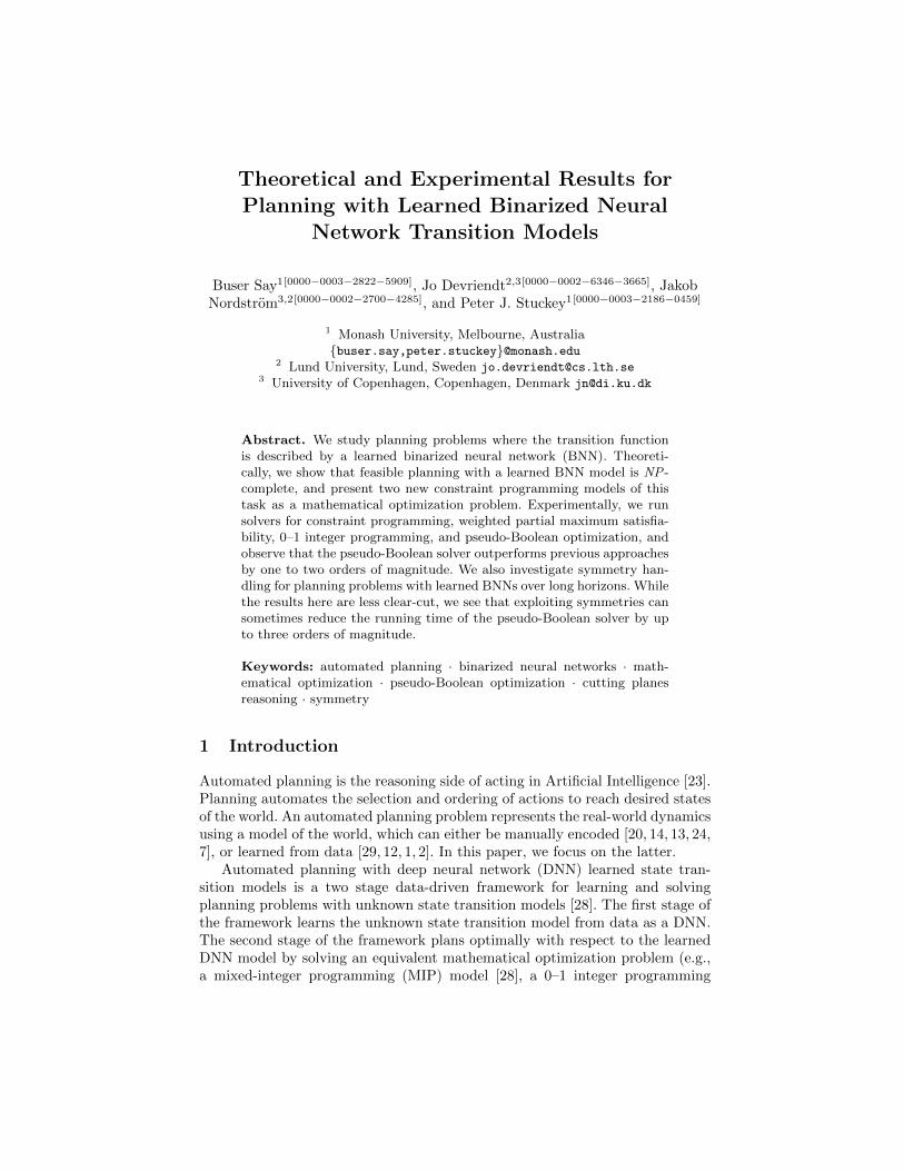
Fig. 1: Learned BNN with two layers L = 2 for the problem in Example 1. Inthis example learned BNN, the input layer J(1) has neurons u1,1 and u2,1 rep-resenting s1 and a1, respectively. The node n2,1 represents batch normalizationfor neuron u2,1. Given the parameter values w1,1,l = 1, w2,1,l = −1, µ1,2 = 0,σ2

1,2 = 2, ε1,2 = 2, γ1,2 = 3 and βj,l = 1, the input x1,2 to neuron u1,2 iscalculated according to the formula specified in Section 2.2.

Batch Normalization Layers. For layers l ∈ {2, . . . , L}, Batch Normaliza-tion [18] transforms the weighted sum of outputs at layer l − 1 in 4j,l =∑i∈J(l−1) wi,j,lyi,l−1 to inputs xj,l of neurons uj,l ∈ J(l) using the formula xj,l =

4j,l−µj,l√σ2j,l+εj,l

γj,l + βj,l, where yi,l−1 denotes the output of neuron ui,l−1 ∈ J(l − 1),

and the parameters are the weight wi,j,l, input mean µj,l, input variance σ2j,l, nu-

merical stability constant εj,l, input scaling γj,l, and input bias βj,l, all computedat training time.

Activation Layers. Given input xj,l, the deterministic activation function yj,lcomputes the output of neuron uj,l ∈ J(l) at layer l ∈ {2, . . . , L}, which is 1if xj,l ≥ 0 and −1 otherwise. The last activation layer consists of neuronsui,L ∈ J(L) that represent the codomain of the learned state transition func-

tion T . We assume neurons u1,L, . . . , un,L ∈ J(L) represent the state variables S.

The proposed BNN architecture is trained to learn the function T from datathat consists of measurements on the domain and codomain of the unknown statetransition function T : Ds1 ×· · ·×Dsn ×Da1 ×· · ·×Dam → Ds1 ×· · ·×Dsn . Anexample learned BNN for the problem of Example 1 is visualized in Figure 1.

3 0–1 Integer Programming Model for the LearnedPlanning Problem

In this section, we present the 0–1 integer programming (IP) model from [25, 26]previously used to solve learned automated planning problems. A 0–1 IP modelcan be solved optimally by a mixed-integer programming (MIP) solver (as waspreviously investigated [25, 26]). Equivalently, this can be viewed as a pseudo-Boolean optimization (PBO) model to be solved using a PBO solver, since allthe variables are 0–1 or equivalently Boolean.


u1,1

u2,1

Layer 1 Layer 2

u1,2

w2,1,2=-1

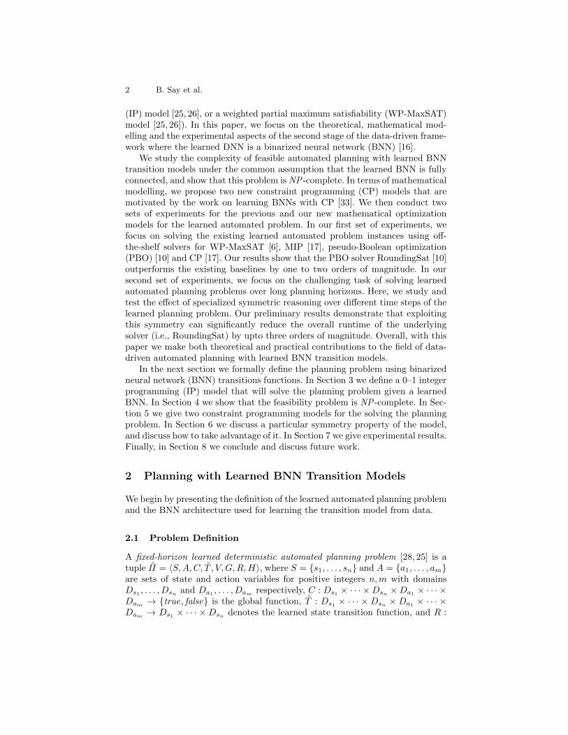
w1,1,2=1B(1,2) = 1 = ⌈ 1 2 + 2

3 − 0⌉

y1,2 = {1, if y1,1 − y2,1 + B(1,2) ≥ 0−1, otherwise

Fig. 2: The visualization of bias computation B(1, 2) for neuron u1,2 ∈ J(2) inthe example learned BNN presented in Figure 1.

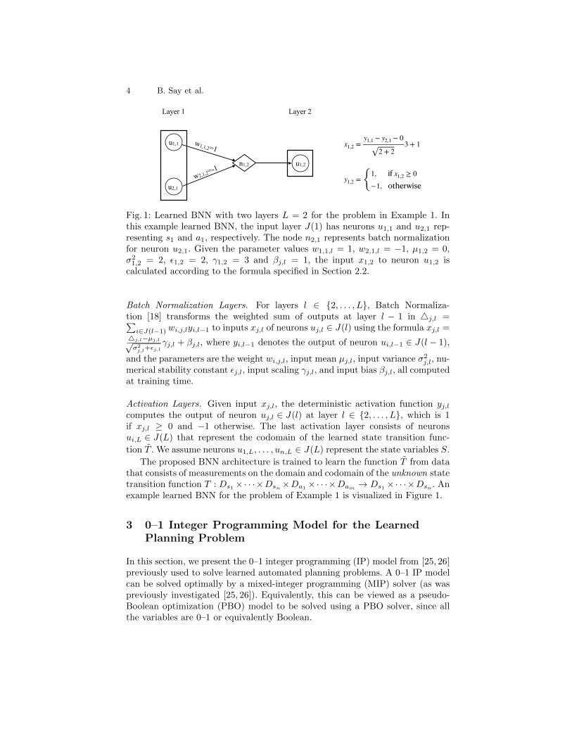
Decision Variables. The 0–1 IP model uses the following decision variables:

– Xi,t encodes whether action ai ∈ A is executed at time step t ∈ {1, . . . ,H}or not.

– Yi,t encodes whether we are in state si ∈ S at time step t ∈ {1, . . . ,H + 1}or not.

– Zi,l,t encodes whether neuron ui,l ∈ J(l) in layer l ∈ {1, . . . , L} is activatedat time step t ∈ {1, . . . ,H} or not.

Parameters. The 0–1 IP model uses the following parameters:

– wi,j,l is the value of the learned BNN weight between neurons ui,l−1 ∈ J(l−1)and uj,l ∈ J(l) in layer l ∈ {2, . . . , L}.

– B(j, l) is the bias of neuron uj,l ∈ J(l) in layer l ∈ {2, . . . , L}. Given thevalues of normalization parameters µj,l, σ

2j,l, εj,l, γj,l and βj,l, the bias is

computed as B(j, l) =

⌈βj,l

√σ2j,l+εj,l

γj,l− µj,l

⌉. The visualization of the calcu-

lation of the bias B(j, l) is presented in Figure 2.

Constraints. The 0–1 IP model has the following constraints:

Yi,1 = Vi ∀si∈S (1)

G(〈Y1,H+1, . . . , Yn,H+1〉) = true (2)

C(〈Y1,t, . . . , Yn,t, X1,t, . . . , Xm,t〉) = true ∀t∈{1,...,H} (3)

Yi,t = Zi,1,t ∀si∈S,t∈{1,...,H} (4)

Xi,t = Zi+n,1,t ∀ai∈A,t∈{1,...,H} (5)

Yi,t+1 = Zi,L,t ∀si∈S,t∈{1,...,H} (6)(B(j, l)− |J(l−1)|

)(1−Zj,l,t

)≤ In(j, l, t) ∀uj,l∈J(l),l∈{2,...,L},t∈{1,...,H} (7)(

B(j, l)+|J(l−1)|+1)Zj,l,t − 1 ≥ In(j, l, t) ∀uj,l∈J(l),l∈{2,...,L},t∈{1,...,H} (8)

where the input expression In(j, l, t) for neuron uj,l ∈ J(l) in layer l ∈ {2, . . . , L}at time step t ∈ {1, . . . ,H} is equal to

∑ui,l−1∈J(l−1) wi,j,l(2·Zi,l−1,t−1)+B(j, l).

6 B. Say et al.

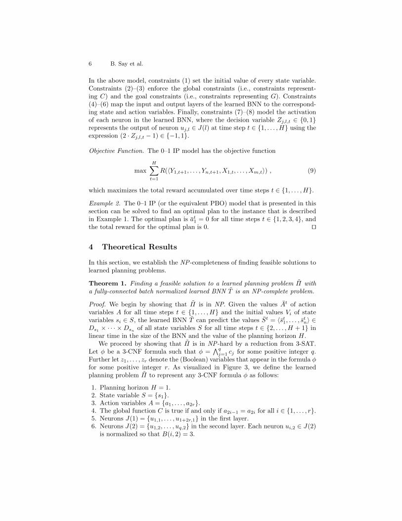
In the above model, constraints (1) set the initial value of every state variable.Constraints (2)–(3) enforce the global constraints (i.e., constraints represent-ing C) and the goal constraints (i.e., constraints representing G). Constraints(4)–(6) map the input and output layers of the learned BNN to the correspond-ing state and action variables. Finally, constraints (7)–(8) model the activationof each neuron in the learned BNN, where the decision variable Zj,l,t ∈ {0, 1}represents the output of neuron uj,l ∈ J(l) at time step t ∈ {1, . . . ,H} using theexpression (2 · Zj,l,t − 1) ∈ {−1, 1}.

Objective Function. The 0–1 IP model has the objective function

max

H∑t=1

R(〈Y1,t+1, . . . , Yn,t+1, X1,t, . . . , Xm,t〉) , (9)

which maximizes the total reward accumulated over time steps t ∈ {1, . . . ,H}.

Example 2. The 0–1 IP (or the equivalent PBO) model that is presented in thissection can be solved to find an optimal plan to the instance that is describedin Example 1. The optimal plan is at1 = 0 for all time steps t ∈ {1, 2, 3, 4}, andthe total reward for the optimal plan is 0. ut

4 Theoretical Results

In this section, we establish the NP -completeness of finding feasible solutions tolearned planning problems.

Theorem 1. Finding a feasible solution to a learned planning problem Π witha fully-connected batch normalized learned BNN T is an NP-complete problem.

Proof. We begin by showing that Π is in NP. Given the values At of actionvariables A for all time steps t ∈ {1, . . . ,H} and the initial values Vi of statevariables si ∈ S, the learned BNN T can predict the values St = 〈st1, . . . , stn〉 ∈Ds1 × · · · ×Dsn of all state variables S for all time steps t ∈ {2, . . . ,H + 1} inlinear time in the size of the BNN and the value of the planning horizon H.

We proceed by showing that Π is in NP -hard by a reduction from 3-SAT.Let φ be a 3-CNF formula such that φ =

∧qj=1 cj for some positive integer q.

Further let z1, . . . , zr denote the (Boolean) variables that appear in the formula φfor some positive integer r. As visualized in Figure 3, we define the learnedplanning problem Π to represent any 3-CNF formula φ as follows:

1. Planning horizon H = 1.2. State variable S = {s1}.3. Action variables A = {a1, . . . , a2r}.4. The global function C is true if and only if a2i−1 = a2i for all i ∈ {1, . . . , r}.5. Neurons J(1) = {u1,1, . . . , u1+2r,1} in the first layer.6. Neurons J(2) = {u1,2, . . . , uq,2} in the second layer. Each neuron ui,2 ∈ J(2)

is normalized so that B(i, 2) = 3.


u1,1

u2i,1

u2i+1,1

Layer 1 Layer 2 Layer 3

uj,2

uk,2

u1,3

.

.

w2i+1,k,2=-1

w2i,k,2=1

w2i+1,j,2=1w2i,j,2=1

.

.

.

.

.

.

.

.

.

.

.

Fig. 3: Visualization of the NP -hardness proof by a reduction from a 3-CNFformula φ =

∧qj=1 cj to the learned planning problem Π. In the first layer,

two neurons u2i,1, u2i+1,1 ∈ J(1) together represent the Boolean variable zifrom the formula φ. When variable zi does not appear in clause ck, the weightsw2i,k,2, w2i+1,k,2 are set so the input to neuron uk,2 ∈ J(2) is cancelled out (i.e.,case (a) of step (7)). In the remaining cases, the weights w2i,j,2, w2i+1,j,2 are setto ensure the input to neuron uj,2 ∈ J(2) is positive if and only if the respectiveliteral that appears in clause cj evaluates to true (e.g., case (c) of step (7) isvisualized).

7. Set the learned weights between neurons u2i,1, u2i+1,1 ∈ J(1)\u1,1 and uj,2 ∈J(2) according to the following rules. (a) If zi does not appear in clause cj ,set w2i,j,2 = 1, w2i+1,j,2 = −1, (b) else if the negation of zi appears in clausecj (i.e., ¬zi), set w2i,j,2 = w2i+1,j,2 = −1, (c) else, set w2i,j,2 = w2i+1,j,2 = 1.

8. Neuron J(3) = {u1,3} in the third layer. Neuron u1,3 is normalized such thatB(1, 3) = −q.

9. Set the learned weights wi,1,3 = 1 between ui,2 ∈ J(2) and u1,3 ∈ J(3).10. The goal state function G is defined as G(〈1〉) = true and G(〈0〉) = false.

In the reduction presented above, step (1) sets the value of the planninghorizon H to 1. Step (2) defines a single state variable s1 to represent whetherthe formula φ is satisfied (i.e., s1 = 1) or not (i.e., s1 = 0). Step (3) definesaction variables a1, . . . , a2r to represent the Boolean variables z1, . . . , zr in theformula φ. Step (4) ensures that the pairs of action variables a2i−1, a2i thatrepresent the same Boolean variable zi take the same value. Step (5) definesthe neurons in the first layer (i.e., l = 1) of the BNN. Step (6) defines theneurons in the second layer (i.e., l = 2) of the BNN. Each neuron ui,2 ∈ J(2)represents a clause ci in the formula φ, and the input of each neuron ui,2 isnormalized so that B(i, 2) = 3. Step (7) defines the weights between the firstand the second layers so that the output of neurons u2i,1, u2i+1,1 ∈ J(1) onlyaffects the input of the neurons uj,2 ∈ J(2) in the second layer if and only if theBoolean variable zi appears in clause cj . When this is not the case, the output

8 B. Say et al.

of neurons u2i,1, u2i+1,1 are cancelled out due to the different values of theirweights, so that w2i,j,2 + w2i+1,j,2 = 0. Steps (6) and (7) together ensure that forany values of V1 and w1,j,2, neuron uj,2 ∈ J(2) is activated if and only if at leastone literal in clause cj evaluates to true.4 Step (8) defines the single neuron inthe third layer (i.e., l = 3) of the BNN. Neuron u1,3 ∈ J(3) predicts the value ofstate variable s1. Step (9) defines the weights between the second and the thirdlayers so that the neuron u1,3 ∈ J(3) activates if and only if all clauses in theformula φ are satisfied. Finally, step (10) ensures that the values of the actionsconstitute a solution to the learned planning problem Π if and only if all clausesare satisfied. ut

5 Constraint Programming Models for the LearnedPlanning Problem

In this section, we present two new constraint programming (CP) models to solvethe learned automated planning problem Π. The models make use of reificationrather than restricting themselves to linear constraints. This allows a more directexpression of the BNN constraints.

5.1 Constraint Programming Model 1

Decision Variables and Parameters. The CP model 1 uses the same set of de-cision variables and parameters as the 0–1 IP model previously described inSection 3.

Constraints. The CP model 1 has the following constraints:

Constraints (1)–(6)

(In(j, l, t) ≥ 0) = Zj,l,t ∀uj,l∈J(l),l∈{2,...,L},t∈{1,...,H} (10)


∑ui,l−1∈J(l−1) wi,j,l(2·Zi,l−1,t−1)+B(j, l).

In the above model, constraint (10) models the activation of each neuron in thelearned BNN by replacing constraints (7)–(8).

Objective Function. The CP model 1 uses the same objective function as the0–1 IP model previously described in Section 3.

4 Each neuron uj,2 that represents clause cj receives seven non-zero inputs (i.e., onefrom state and six from action variables). The bias B(j, 2) is set so that the activationcondition holds when at least one literal in clause cj evaluates to true. For example,the constraint −2+w1,j,2V1+B(j, 2) ≥ 0 represents the case when exactly one literalin clause cj evaluates to true where the terms −2 and w1,j,2V1 represent the inputsfrom the six action variables and the single state variable, respectively. Similarly, theconstraint −6 + w1,j,2V1 + B(j, 2) < 0 represents the case when all literals in clausecj evaluate to false and the activation condition does not hold.


5.2 Constraint Programming Model 2

Decision Variables. The CP model 2 uses the Xi,t and Yi,t decision variablespreviously described in Section 3.

Parameters. The CP model 2 uses the same set of parameters as the 0–1 IPmodel previously described in Section 3.

Constraints. The CP model 2 has the following constraints:

Constraints (1)–(6)

(In(j, l, t) ≥ 0) = Expr j,l,t ∀uj,l∈J(l),l∈{2,...,L},t∈{1,...,H} (11)


∑ui,l−1∈J(l−1) wi,j,l(2 · Expr i,l−1,t − 1) +

B(j, l), and output expression Expr j,l,t represents the binary output of neuronuj,l ∈ J(l) in layer l ∈ {2, . . . , L} at time step t ∈ {1, . . . ,H}. In the abovemodel, constraint (11) models the activation of each neuron in the learned BNNby replacing the decision variable Zj,l,t in constraint (10) with the expressionExpr j,l,t The difference between an integer variable and an expression is thatduring solving the solver does not store the domain (current set of possiblevalues) for an expression. Expressions allow more scope for the presolve of CPOptimizer [17] to rewrite the constraints to a more suitable form, and allow theuse of more specific propagation scheduling.

Objective Function. The CP model 2 uses the same objective function as the0–1 IP model that is previously described in section 3.

6 Model Symmetry

Examining the 0–1 IP (or equivalently the PBO) model, one can see the bulkof the model involves copies of the learned BNN constraints over all time steps.These constraints model the activation of each neuron (i.e., constraints (4)–(8))and constrain the input of the BNN (i.e., constraint (3)). The remainder of themodel is constraints on the initial and goal states (i.e., constraints (1)–(2)). Soif we ignore the initial and goal state constraints, the model is symmetric overthe time steps. Note that this symmetry property is not a global one: the modelis not symmetric as a whole. Rather, this local symmetry arises because subsetsof constraints are isomorphic to each other. Because of this particular formof symmetry, the classic approach of adding symmetry breaking predicates [5]would not be sound, as this requires global symmetry.

Instead, we exploit this symmetry by deriving symmetric nogoods on-the-fly. If a nogood is derived purely from constraints (3)–(8), and if a sufficientlysmall subset of time steps was involved in its derivation, then we can shift thetime steps of this nogood over the planning horizon, learning a valid symmetricnogood. To track which constraints a nogood is derived from, we use the SAT

10 B. Say et al.

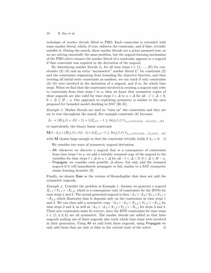
technique of marker literals lifted to PBO. Each constraint is extended withsome marker literal, which, if true, enforces the constraint, and if false, triviallysatisfies it. During the search, these marker literals are a priori assumed true, sowe are solving essentially the same problem, but the nogood learning mechanismof the PBO solver ensures the marker literal of a constraint appears in a nogoodif that constraint was required in the derivation of the nogood.

By introducing marker literals Lt for all time steps t ∈ {1, . . . ,H} for con-straints (3)–(8) and an extra “asymmetric” marker literal L∗ for constraint (2)and the constraints originating from bounding the objective function, and thentreating all initial state constraints as markers, we can track if only constraints(3)–(8) were involved in the derivation of a nogood, and if so, for which timesteps. When we find that the constraints involved in creating a nogood only referto constraints from time steps l to u, then we know that symmetric copies ofthese nogoods are also valid for time steps l +∆ to u+∆ for all −l < ∆ < 0,0 < ∆ ≤ H − u. Our approach to exploiting symmetry is similar to the onesproposed for bounded model checking in SAT [30, 31].

Example 3. Marker literals are used to “turn on” the constraints and they areset to true throughout the search. For example constraint (8) becomes

Lt → (B(j, l) + J(l − 1) + 1)Zj,l,t − 1 ≥ In(j, l, t) ∀uj,l∈J(l),l∈{2,...,L},t∈{1,...,H}

or equivalently, the binary linear constraint

M(1−Lt)+(B(j, l)+J(l−1)+1)Zj,l,t−1 ≥ In(j, l, t) ∀uj,l∈J(l),l∈{2,...,L},t∈{1,...,H}

with M chosen large enough so that the constraint trivially holds if Lt = 0. utWe consider two ways of symmetric nogood derivation:

– All: whenever we discover a nogood that is a consequence of constraintsfrom time steps l to u, we add a suitably renamed copy of the nogood to thevariables for time steps l +∆ to u+∆ for all −l < ∆ < 0, 0 < ∆ ≤ H − u,

– Propagate: we consider each possible ∆ above, but only add the renamednogood if it will immediately propagate or fail, similar to a SAT symmetricclause learning heuristic [8].

Finally, we denote Base as the version of RoundingSat that does not add thesymmetric nogoods.

Example 4. Consider the problem in Example 1. Assume we generate a nogoodX1,1 ∨ Y1,1 ∨¬X1,2, which is a consequence only of constraints for the BNNs fortime steps 1 and 2. The actual generated nogood is then ¬L1∨¬L2∨X1,1∨Y1,1∨¬X1,2 which illustrates that it depends only on the constraints in time steps 1and 2. We can then add a symmetric copy ¬L2 ∨ ¬L3 ∨X1,2 ∨ Y1,2 ∨ ¬X1,3 fortime steps 2 and 3, as well as ¬L3 ∨¬L4 ∨X1,3 ∨ Y1,3 ∨¬X1,4 for steps 3 and 4.These new constraints must be correct, since the BNN constraints for time stepst ∈ {1, 2, 3, 4} are all symmetric. The marker literals are added so that laternogoods making use of these nogoods also track which time steps were involvedin their generation. Using All we add both these nogoods, using Propagate weonly add those that are unit or false in the current state of the solver. ut


Fig. 4: Cumulative number of problems solved by IP (blue), WP-MaxSAT (red),CP1 (green), CP2 (black) and PBO (orange) models over 27 instances of theproblem Π within the time limit.

7 Experimental Results

In this section, we present results on two sets of computational experiments.In the first set of experiments, we compare different approaches to solving thelearned planning problem Π with mathematical optimization models. In thesecond set of experiments, we present preliminary results on the effect of derivingsymmetric nogoods when solving Π over long horizons H.

7.1 Experiments 1

We first experimentally test the runtime efficiency of solving the learned planningproblem Π with mathematical optimization models using off-the-shelf solvers.All the existing benchmark instances of the learned planning problem Π (i.e., 27in total) were used [26]. We ran the experiments on a MacBookPro with 2.8 GHzIntel Core i7 16GB memory, with one hour total time limit per instance. We usedthe MIP solver CPLEX 12.10 [17] to optimize the 0–1 IP model, MaxHS [6]with underlying CPLEX 12.10 linear programming solver to optimize the WP-MaxSAT model [26], and CP Optimizer 12.10 [17] to optimize the CP Model 1(CP1) and the CP Model 2 (CP2). Finally, we optimized a pseudo-Booleanoptimization (PBO) model, which simply replaces all binary variables in the 0–1IP model with Boolean variables, using RoundingSat [10].

In Figure 4, we visualize the cumulative number of problems solved by allfive models, namely: IP (blue), WP-MaxSAT (red), CP1 (green), CP2 (black)and PBO (orange), over 27 instances of the learned planning problem Π withinone hour time limit. Figure 4 clearly highlights the experimental efficiency ofsolving the PBO model. We find that using the PBO model with RoundingSatsolves all existing benchmarks under 1000 seconds. In contrast, we observe thatthe 0–1 IP model performs poorly, with only 19 instances out of 27 solved withinthe one hour time limit. The remaining three models, WP-MaxSAT, CP1 and

12 B. Say et al.

(a) CP1 vs. CP2 (b) WP-MaxSAT vs. CP1 (c) WP-MaxSAT vs. CP2

Fig. 5: Pairwise runtime comparison between WP-MaxSAT, CP1 and CP2 mod-els over 27 instances of problem Π within the time limit.

CP2, demonstrate relatively comparable runtime performance, which we explorein more detail next.

In Figures 5a, 5b and 5c, we present scatter plots comparing the WP-MaxSAT, CP1 and CP2 models. In each figure, each dot (red) represents aninstance of the learned planning problem Π and each axis represents a model(i.e., WP-MaxSAT, CP1 or CP2). If a dot falls below the diagonal line (blue),it means the corresponding instance is solved faster by the model representedby the y-axis than the one represented by the x-axis. In Figure 5a, we comparethe two CP models CP1 and CP2. A detailed inspection of Figure 5a shows acomparable runtime performance on the instances that take less than 1000 sec-onds to solve (i.e., most dots fall closely to the diagonal line). In the remainingtwo instances that are solved by CP2 under 1000 seconds, CP1 runs out of theone hour time limit. These results suggest that using expressions instead of deci-sion variables to model the neurons of the learned BNN allows the CP solver tosolve harder instances (i.e., instances that take more than 1000 seconds to solve)more efficiently. In Figures 5b and 5c, we compare CP1 and CP2 against theWP-MaxSAT model, respectively. Both figures show a similar trend on runtimeperformance; the CP models close instances that take less than 1000 seconds tosolve by one to two orders of magnitude faster than the WP-MaxSAT model, andthe WP-MaxSAT model performs comparably to the CP models on the harderinstances. Overall, we find that WP-MaxSAT solves one more and one less in-stances compared to CP1 and CP2 within the one hour time limit, respectively.These results suggest that the WP-MaxSAT model pays a heavy price for thelarge size of its compilation when the instances take less than 1000 seconds tosolve, and only benefits from its SAT-based encoding for harder instances.

Next, we compare the runtime performance of WP-MaxSAT, CP1 and CP2against the best performing model (i.e., PBO) in more detail in Figures 6a,6b and 6c. These plots show that the PBO model significantly outperformsthe WP-MaxSAT, CP1 and CP2 models across all instances. Specifically, Fig-ure 6a shows that the PBO model is better than the previous state-of-the-art


(a) PBO vs. WP-MaxSAT (b) PBO vs. CP1 (c) PBO vs. CP2

Fig. 6: Pairwise runtime comparison between PBO, and WP-MaxSAT, CP1 andCP2 models over 27 instances of problem Π within the time limit.

WP-MaxSAT model across all instances by one to two orders of magnitude interms of runtime performance. Similarly, Figures 6b and 6c show that the PBOmodel outperforms both CP models across all instances, except in one and twoinstances, respectively, by an order of magnitude.

It is interesting that the 0–1 IP model works so poorly for the MIP solver,while the equivalent PBO model is solved efficiently using a PBO solver. It seemsthat the linear relaxations used by the MIP solver are too weak to generate usefulinformation, and it ends up having to fix activation variables in order to reasonmeaningfully. In contrast, it appears that the PBO solver is able to determinesome useful information from the neuron constraints without necessarily fixingthe activation variables—probably since it uses integer-based cutting planes rea-soning [4] rather than continuous linear programming reasoning for the linearexpressions—and the nogood learning helps it avoid repeated work.

7.2 Experiments 2

We next evaluate the effect of symmetric nogood derivation on solving thelearned planning problem Π over long horizons H. For these experiments, wegenerated instances by incrementing the value of the planning horizon H in thebenchmark instances in Section 7.1, and used the same hardware and time limitsettings. We modified the best performing solver RoundingSat [10] to includesymmetry reasoning as discussed in Section 6.

In Figure 7, we visualize the cumulative number of problems solved for allthree versions of RoundingSat, namely Base (blue), Propagate (red), and All(black), over 21 instances of the learned planning problem Π over long hori-zons H within one hour time limit. Figure 7 demonstrates that symmetric no-good derivation can improve the efficiency of solving the underlying PBO model.We find that Propagate solves the most instances within the time limit. A moredetailed inspection of the results further suggests that between the remainingtwo version of RoundingSat, All solves more instances faster compared to Base.

14 B. Say et al.

Fig. 7: Cumulative number of problems solved for Base (blue), Propagate (red)and All (black) models over 21 instances of the problem Π within the time limit.

(a) Base vs. Propagate (b) Base vs. All (c) Propagate vs. All

Fig. 8: Pairwise runtime comparison between Base, Propagate and All modelsover 21 instances of problem Π within the time limit.

Next, in Figures 8a, 8b and 8c, we explore the pairwise runtime compar-isons of the three versions of RoundingSat in more detail. In Figures 8a and 8b,we compare Propagate and All against Base, respectively. It is clear from thesescatter plots that Propagate and All outperform Base in terms of runtime per-formance. Specifically, in Figure 8b, we find that All outperforms Base by up tothree orders of magnitude in terms of runtime performance. Finally, in Figure 8c,we compare the two versions of RoundingSat that are enhanced with symmetricnogood derivation. A detailed inspection of Figure 8c reveals that All is slightlyfaster than Propagate in general.

8 Related Work, Conclusions and Future Work

In this paper, we studied the important problem of automated planning withlearned BNNs, and made four important contributions. First, we showed thatthe feasibility problem is NP -complete. Unlike the proof presented for the task


of verifying learned BNNs [3], our proof does not rely on setting weights to zero(i.e., sparsification). Instead, our proof achieves the same expressivity for fullyconnected BNN architectures, without adding additional layers or increasingthe width of the layers,by representing each input with two copies of actionvariables. Second, we introduced two new CP models for the problem. Third, wepresented detailed computational results for solving the existing instances of theproblem. Lastly, we studied the effect of deriving symmetric nogoods on solvingnew instances of the problem with long horizons.

It appears that BNN models provide a perfect class of problems for pseudo-Boolean solvers, since each neuron is modelled by pseudo-Boolean constraints,but the continuous relaxation is too weak for MIP solvers to take advantage of,while propagation-based approaches suffer since they are unable to reason aboutlinear expressions directly. PBO solvers directly reason about integer (0–1) linearexpressions, making them very strong on this class of problems.

Our results have the potential to improve other important tasks with learnedBNNs (and other DNNs), such as automated planning in real-valued action andstate spaces [35, 27, 36], decision making in discrete action and state spaces [21],goal recognition [11], training [33], verification [19, 9, 15, 22], robustness evalua-tion [32] and defenses to adversarial attacks [34], which rely on efficiently solvingsimilar problems that we solve in this paper. The derivation of symmetric no-goods is a promising avenue for future work, in particular, if a sufficient numberof symmetric nogoods can be generated. Relating the number of derived sym-metric nogoods to the wall-clock speed-up of the solver or the reduction of thesearch tree might shed further light on the efficacy of this approach.

Acknowledgements

Some of our preliminary computational experiments used resources provided bythe Swedish National Infrastructure for Computing (SNIC) at the High Perfor-mance Computing Center North (HPC2N) at Umea University. Jo Devriendtand Jakob Nordstrom were supported by the Swedish Research Council grant2016-00782, and Jakob Nordstrom also received funding from the IndependentResearch Fund Denmark grant 9040-00389B.

References

1. Bennett, S.W., DeJong, G.F.: Real-world robotics: Learning to plan for robustexecution. In: Machine Learning. vol. 23, pp. 121–161 (1996)

2. Benson, S.S.: Learning Action Models for Reactive Autonomous Agents. Ph.D.thesis, Stanford University, Stanford, CA, USA (1997)

3. Cheng, C.H., Nuhrenberg, G., Huang, C.H., Ruess, H.: Verification of binarizedneural networks via inter-neuron factoring. In: Piskac, R., Rummer, P. (eds.) Ver-ified Software. Theories, Tools, and Experiments. pp. 279–290. Springer Interna-tional Publishing, Cham (2018)

4. Cook, W., Coullard, C.R., Turan, G.: On the complexity of cutting-plane proofs.Discrete Applied Mathematics 18(1), 25–38 (1987)

16 B. Say et al.

5. Crawford, J., Ginsberg, M., Luks, E., Roy, A.: Symmetry-breaking predicates forsearch problems. In: Proceedings of the Fifth International Conference on Princi-ples of Knowledge Representation and Reasoning. pp. 148–159. Morgan Kaufmann(1996)

6. Davies, J., Bacchus, F.: Solving MAXSAT by solving a sequence of simpler SATinstances. In: Lee, J. (ed.) Principles and Practice of Constraint Programming. pp.225–239. CP 2011, Springer Berlin Heidelberg, Berlin, Heidelberg (2011)

7. Davies, T.O., Pearce, A.R., Stuckey, P.J., Lipovetzky, N.: Sequencing operatorcounts. In: Proceedings of the Twenty-Fifth International Conference on Auto-mated Planning and Scheduling. pp. 61–69. AAAI Press (2015)

8. Devriendt, J., Bogaerts, B., Bruynooghe, M.: Symmetric explanation learning: Ef-fective dynamic symmetry handling for SAT. In: Gaspers, S., Walsh, T. (eds.)Theory and Applications of Satisfiability Testing – SAT 2017. pp. 83–100. SpringerInternational Publishing, Cham (2017)

9. Ehlers, R.: Formal verification of piece-wise linear feed-forward neural networks.In: D’Souza, D., Narayan Kumar, K. (eds.) Automated Technology for Verificationand Analysis. pp. 269–286. Springer International Publishing, Cham (2017)

10. Elffers, J., Nordstrom, J.: Divide and conquer: Towards faster pseudo-boolean solv-ing. In: Proceedings of the Twenty-Seventh International Joint Conference on Ar-tificial Intelligence. pp. 1291–1299. IJCAI’18 (2018)

11. Fraga Pereira, R., Vered, M., Meneguzzi, F., Ramırez, M.: Online probabilisticgoal recognition over nominal models. In: Proceedings of the Twenty-Eighth Inter-national Joint Conference on Artificial Intelligence. pp. 5547–5553. InternationalJoint Conferences on Artificial Intelligence Organization (2019)

12. Gil, Y.: Acquiring Domain Knowledge for Planning by Experimentation. Ph.D.thesis, Carnegie Mellon University, USA (1992)

13. Helmert, M.: The fast downward planning system. In: Journal Artificial IntelligenceResearch. vol. 26, pp. 191–246. AI Access Foundation, USA (2006)

14. Hoffmann, J., Nebel, B.: The FF planning system: Fast plan generation throughheuristic search. In: Journal of Artificial Intelligence Research. vol. 14, pp. 253–302.AI Access Foundation, USA (2001)

15. Huang, X., Kwiatkowska, M., Wang, S., Wu, M.: Safety verification of deep neuralnetworks. In: Majumdar, R., Kuncak, V. (eds.) Computer Aided Verification. pp.3–29. Springer International Publishing, Cham (2017)

16. Hubara, I., Courbariaux, M., Soudry, D., El-Yaniv, R., Bengio, Y.: Binarized neuralnetworks. In: Proceedings of the Thirtieth International Conference on NeuralInformation Processing Systems. pp. 4114–4122. NIPS’16, Curran Associates Inc.,USA (2016)

17. IBM: IBM ILOG CPLEX Optimization Studio CPLEX User’s Manual (2020)18. Ioffe, S., Szegedy, C.: Batch normalization: Accelerating deep network training by

reducing internal covariate shift. In: Proceedings of the Thirty-Second InternationalConference on International Conference on Machine Learning. pp. 448–456. ICML,JMLR.org (2015)

19. Katz, G., Barrett, C., Dill, D., Julian, K., Kochenderfer, M.: Reluplex: An efficientSMT solver for verifying deep neural networks. In: Proceedings of the Twenty-Ninth International Conference on Computer Aided Verification. CAV (2017)

20. Kautz, H., Selman, B.: Planning as satisfiability. In: Proceedings of the TenthEuropean Conference on Artificial Intelligence. pp. 359–363. ECAI’92 (1992)

21. Lombardi, M., Gualandi, S.: A Lagrangian propagator for artificial neural networksin constraint programming. In: Constraints. vol. 21, pp. 435–462 (2016)


22. Narodytska, N., Kasiviswanathan, S., Ryzhyk, L., Sagiv, M., Walsh, T.: Verifyingproperties of binarized deep neural networks. In: Proceedings of the Thirty-SecondAAAI Conference on Artificial Intelligence. pp. 6615–6624 (2018)

23. Nau, D., Ghallab, M., Traverso, P.: Automated Planning: Theory & Practice. Mor-gan Kaufmann Publishers Inc., San Francisco, CA, USA (2004)

24. Pommerening, F., Roger, G., Helmert, M., Bonet, B.: LP-based heuristics for cost-optimal planning. In: Proceedings of the Twenty-Fourth International Conferenceon Automated Planning and Scheduling. pp. 226–234. ICAPS’14, AAAI Press(2014)

25. Say, B., Sanner, S.: Planning in factored state and action spaces with learnedbinarized neural network transition models. In: Proceedings of the Twenty-SeventhInternational Joint Conference on Artificial Intelligence. pp. 4815–4821. IJCAI’18(2018)

26. Say, B., Sanner, S.: Compact and efficient encodings for planning in factored stateand action spaces with learned binarized neural network transition models. Artifi-cial Intelligence 285, 103291 (2020)

27. Say, B., Sanner, S., Thiebaux, S.: Reward potentials for planning with learnedneural network transition models. In: Schiex, T., de Givry, S. (eds.) Proceedings ofthe Twenty-Fifth International Conference on Principles and Practice of ConstraintProgramming. pp. 674–689. Springer International Publishing, Cham (2019)

28. Say, B., Wu, G., Zhou, Y.Q., Sanner, S.: Nonlinear hybrid planning with deep netlearned transition models and mixed-integer linear programming. In: Proceedingsof the Twenty-Sixth International Joint Conference on Artificial Intelligence. pp.750–756. IJCAI’17 (2017)

29. Shen, W.M., Simon, H.A.: Rule creation and rule learning through environmentalexploration. In: Proceedings of the Eleventh International Joint Conference onArtificial Intelligence. pp. 675—-680. IJCAI’89, Morgan Kaufmann Publishers Inc.,San Francisco, CA, USA (1989)

30. Shtrichman, O.: Tuning SAT checkers for bounded model checking. In: Emerson,E.A., Sistla, A.P. (eds.) Computer Aided Verification. pp. 480–494. Springer BerlinHeidelberg, Berlin, Heidelberg (2000)

31. Shtrichman, O.: Pruning techniques for the SAT-based bounded model checkingproblem. In: Margaria, T., Melham, T. (eds.) Correct Hardware Design and Veri-fication Methods. pp. 58–70. Springer Berlin Heidelberg, Berlin, Heidelberg (2001)

32. Tjeng, V., Xiao, K., Tedrake, R.: Evaluating robustness of neural networks withmixed integer programming. In: Proceedings of the Seventh International Confer-ence on Learning Representations. ICLR (2019)

33. Toro Icarte, R., Illanes, L., Castro, M.P., Cire, A.A., McIlraith, S.A., Beck, J.C.:Training binarized neural networks using MIP and CP. In: Schiex, T., de Givry, S.(eds.) Principles and Practice of Constraint Programming. pp. 401–417. SpringerInternational Publishing, Cham (2019)

34. Wong, E., Kolter, Z.: Provable defenses against adversarial examples via the con-vex outer adversarial polytope. In: Proceedings of the Thirty-Fifth InternationalConference on Machine Learning. ICML (2018)

35. Wu, G., Say, B., Sanner, S.: Scalable planning with tensorflow for hybrid nonlineardomains. In: Proceedings of the Thirty First Annual Conference on Advances inNeural Information Processing Systems. Long Beach, CA (2017)

36. Wu, G., Say, B., Sanner, S.: Scalable planning with deep neural network learnedtransition models. Journal of Artificial Intelligence Research 68, 571–606 (2020)

Documents

Theoretical and Experimental Results for Planning with