The Need for Structure in Quantum Speedups

Scott Aaronson∗

MIT

Andris Ambainis†

University of Latvia and IAS, Princeton

Abstract

Is there a general theorem that tells us when we can hope for exponential speedups fromquantum algorithms, and when we cannot? In this paper, we make two advances toward sucha theorem, in the black-box model where most quantum algorithms operate.

First, we show that for any problem that is invariant under permuting inputs and outputsand that has sufficiently many outputs (like the collision and element distinctness problems), thequantum query complexity is at least the 7th root of the classical randomized query complexity.(An earlier version of this paper gave the 9th root.) This resolves a conjecture of Watrous from2002.

Second, inspired by work of O’Donnell et al. (2005) and Dinur et al. (2006), we conjecturethat every bounded low-degree polynomial has a “highly influential” variable. Assuming thisconjecture, we show that every T -query quantum algorithm can be simulated on most inputsby a TO(1)-query classical algorithm, and that one essentially cannot hope to prove P 6= BQP

relative to a random oracle.

1 Introduction

Perhaps the central lesson gleaned from fifteen years of quantum algorithms research is this:

Quantum computers can offer superpolynomial speedups over classical computers, butonly for certain “structured” problems.

The key question, of course, is what we mean by “structured.” In the context of most existingquantum algorithms, “structured” basically means that we are trying to determine some globalproperty of an extremely long sequence of numbers, assuming that the sequence satisfies someglobal regularity. As a canonical example, consider Period-Finding, the core of Shor’s algorithmsfor factoring and computing discrete logarithms [29]. Here we are given black-box access to anexponentially-long sequence of integers X = (x1, . . . , xN ); that is, we can compute xi for a giveni. We are asked to find the period of X—that is, the smallest k > 0 such that xi = xi−k forall i > k—promised that X is indeed periodic, with period k ≪ N (and also that the xi valuesare approximately distinct within each period). The requirement of periodicity is crucial here:

∗MIT. Email: aaronson@csail.mit.edu. This material is based upon work supported by the National ScienceFoundation under Grant No. 0844626, by a TIBCO Career Development Chair, and by an Alan T. Waterman award.

†Email: ambainis@lu.lv. Supported by University of Latvia Research Grant ZP01-100, FP7 Marie Curie Inter-national Reintegration Grant (PIRG02-GA-2007-224886), FP7 FET-Open project QCS and ERC Advanced GrantMQC (at the University of Latvia) and the National Science Foundation under agreement No. DMS-1128155 (atIAS, Princeton). Any opinions, findings and conclusions or recommendations expressed in this material are those ofthe author(s) and do not necessarily reflect the views of the National Science Foundation.

1

it is what lets us use the Quantum Fourier Transform to extract the information we want from asuperposition of the form

1√N

N∑

i=1

|i〉 |xi〉 .

For other known quantum algorithms, X needs to be (for example) a cyclic shift of quadraticresidues [16], or constant on the cosets of a hidden subgroup.

By contrast, the canonical example of an “unstructured” problem is the Grover search problem.Here we are given black-box access to an N -bit string (x1, . . . , xN ) ∈ 0, 1N , and are askedwhether there exists an i such that xi = 1.1 Grover [20] gave a quantum algorithm to solve thisproblem using O(

√N) queries [20], as compared to the Ω (N) needed classically. However, this

quadratic speedup is optimal, as shown by Bennett, Bernstein, Brassard, and Vazirani [10]. Forother “unstructured” problems—such as computing the Parity or Majority of an N -bit string—quantum computers offer no asymptotic speedup at all over classical computers (see Beals et al.[8]).

Unfortunately, this “need for structure” has essentially limited the prospects for superpolyno-mial quantum speedups to those areas of mathematics that are liable to produce things like periodicsequences or sequences of quadratic residues.2 This is the fundamental reason why the greatestsuccesses of quantum algorithms research have been in cryptography, and specifically in number-theoretic cryptography. It helps to explain why we do not have a fast quantum algorithm to solveNP-complete problems (for example), or to break arbitrary one-way functions.

Given this history, the following problem takes on considerable importance:

Problem 1 (Informal) For every “unstructured” problem f , are the quantum query complexityQ(f) and the classical randomized query complexity R(f) polynomially related?

Despite its apparent vagueness, Problem 1 can be formalized in several natural and convincingways—and under these formalizations, the problem has remained open for about a decade.

1.1 Formalizing the Problem

Let S ⊆ [M ]N be a collection of inputs, and let f : S → 0, 1 be a function that we are trying tocompute. In this paper, we assume for simplicity that the range of f is 0, 1; in other words, thatwe are trying to solve a decision problem. It will also be convenient to think of f as a functionfrom [M ]N to 0, 1, ∗, where ∗ means ‘undefined’ (that is, that a given input X ∈ [M ]N is not inf ’s domain S).

We will work in the well-studied decision-tree model. In this model, given an input X =(x1, . . . , xN ), an algorithm can at any time choose an i and receive xi. We count only the number ofqueries the algorithm makes to the xi’s, ignoring other computational steps. Then the deterministicquery complexity of f , or D(f), is the number of queries made by an optimal deterministic algorithmon a worst-case input X ∈ S. The (bounded-error) randomized query complexity R(f) is theexpected number of queries made by an optimal randomized algorithm that, for every X ∈ S,computes f(X) with probability at least 2/3. The (bounded-error) quantum query complexity Q(f)is the same as R(f), except that we allow quantum algorithms. Clearly Q(f) ≤ R(f) ≤ D(f) ≤ N

1A variant asks us to find an i such that xi = 1, under the mild promise that such an i exists.2Here we exclude BQP-complete problems, such as simulating quantum physics (the “original” application of

quantum computers), approximating the Jones polynomial [4], and estimating a linear functional of the solution of awell-conditioned linear system [21].

2

for all f . See Buhrman and de Wolf [15] for detailed definitions as well as a survey of thesemeasures.

If S = [M ]N , then we say f is total, and if M = 2, then we say f is Boolean. The case of totalf is relatively well-understood. Already in 1998, Beals et al. [8] showed the following:

Theorem 2 (Beals et al.) D(f) = O(Q(f)6) for all total Boolean functions f : 0, 1N → 0, 1.

Furthermore, it is easy to generalize Theorem 2 to show that D (f) = O(Q(f)6) for all totalfunctions f : [M ]N → 0, 1, not necessarily Boolean.3 In other words, for total functions, thequantum query complexity is always at least the 6th root of the classical query complexity. Thelargest known gap between D(f) and Q(f) for a total function is quadratic, and is achieved by theOR function (because of Grover’s algorithm).

On the other hand, as soon as we allow non-total functions, we can get enormous gaps. Aaron-son [2] gave a Boolean function f : S → 0, 1 for which R(f) = NΩ(1), yet Q(f) = O (1).4 Otherexamples, for which R(f) = Ω(

√N) and Q(f) = O(logN log logN), follow easily from Simon’s al-

gorithm [30] and Shor’s algorithm [29]. Intuitively, these functions f achieve such large separationsby being highly structured: that is, their domain S includes only inputs that satisfy a stringentpromise, such as encoding a periodic function, or (in the case of [2]) encoding two Boolean functions,one of which is correlated with the Fourier transform of the other one.

By contrast with these highly-structured problems, consider the collision problem: that ofdeciding whether a sequence of numbers (x1, . . . , xN ) ∈ [M ]N is one-to-one (each number appearsonce) or two-to-one (each number appears twice). Let Col(X) = 0 if X is one-to-one andCol(X) = 1 if X is two-to-one, promised that one of these is the case. Then Col(X) is nota total function, since its definition involves a promise on X. Intuitively, however, the collisionproblem seems much less “structured” than Simon’s and Shor’s problems. One way to formalizethis intuition is as follows. Call a partial function f : [M ]N → 0, 1, ∗ permutation-invariant if

f(x1, . . . , xN ) = f(τ(xσ(1)), . . . , τ(xσ(N)))

for all inputs X ∈ [M ]N and all permutations σ ∈ SN and τ ∈ SM . Then Col(X) is permutation-invariant: we can permute a one-to-one sequence and relabel its elements however we like, but itis still a one-to-one sequence, and likewise for a two-to-one sequence. Because of this symmetry,attempts to solve the collision problem using (for example) the Quantum Fourier Transform seemunlikely to succeed. And indeed, in 2002 Aaronson [1] proved that Q (Col) = Ω(N1/5): thatis, the quantum query complexity of the collision problem is at most polynomially better thanits randomized query complexity of Θ(

√N). The quantum lower bound was later improved to

Ω(N1/3) by Aaronson and Shi [3], matching an upper bound of Brassard, Høyer, and Tapp [13].Generalizing boldly from this example, John Watrous (personal communication) conjectured

that the randomized and quantum query complexities are polynomially related for every permutation-invariant problem:

3Theorem 2 is proved by combining three ingredients: D(f) = O (C(f) bs(f)), C(f) = O(bs(f)2), and bs(f) =O(Q(f)2) (where C(f) is the certificate complexity of f and bs(f) is the block sensitivity). And all three ingredientsgo through with no essential change if we set M > 2, and define suitable M -ary generalizations of C(f) and bs(f).(We could also convert the non-Boolean function f : [M ]N → 0, 1 to a Boolean one, but then we would lose a factorof logM .)

4Previously, de Beaudrap, Cleve, and Watrous [9] had stated a similar randomized versus quantum separation.However, their separation applied not to the standard quantum black-box model, but to a different model in whichthe black box permutes the answer register |y〉 in some unknown way (rather than simply mapping |y〉 to |y ⊕ f (x)〉).

3

Conjecture 3 (Watrous 2002) R(f) ≤ Q(f)O(1) for every partial function f : [M ]N → 0, 1, ∗that is permutation-invariant.

Let us make two remarks about Conjecture 3. First, the conjecture talks about randomizedversus quantum query complexity, since in this setting, it is easy to find functions f for which R(f)and Q(f) are both tiny but D(f) is huge. As an example, consider the Deutsch-Jozsa problem[17]: given a Boolean input (x1, . . . , xN ), decide whether the xi’s are all equal or whether half ofthem are 1 and the other half are 0, under the promise that one of these is the case.

Second, if M = 2 (that is, f is Boolean), then Conjecture 3 follows relatively easily from knownresults: indeed, we prove in Appendix 6 that R(f) = O(Q(f)2) in that case. So the interestingcase is when M ≫ 2, as it is for the collision problem.

Conjecture 3 provides one natural way to formalize the idea that classical and quantum querycomplexities should be polynomially related for all “unstructured” problems. A different way isprovided by the following conjecture, which we were aware of since about 1999:

Conjecture 4 (folklore) Let Q be a quantum algorithm that makes T queries to a Boolean inputX = (x1, . . . , xN ), and let ε > 0. Then there exists a deterministic classical algorithm that makespoly(T, 1/ε, 1/δ) queries to the xi’s, and that approximates Q’s acceptance probability to within anadditive error ε on a 1− δ fraction of inputs.

But what exactly does Conjecture 4 have to do with “the need for structure in quantumspeedups”? With Conjecture 3, the connection to this paper’s theme was more-or-less obvious,but with Conjecture 4, some additional explanation is probably needed.

Intuitively, we want to say the following: in order to achieve a superpolynomial speedup inthe black-box model, a quantum computer needs not merely a promise problem, but a “severelyconstrained” promise problem. In other words, only a minuscule fraction of the 2N oracle stringsX = (x1, . . . , xN ) ought to satisfy the promise—precisely like what happens in Simon’s and Shor’sproblems, where the promise asserts that X encodes a periodic function. If the promise is too“mild”—if, say, it holds for all X in some set S ⊆ 0, 1N with |S| = Ω(2N )—then we should beback in the situation studied by Beals et al. [8], where the oracle X lacked enough “structure”for a Shor-like algorithm to exploit, and as a result, the best one could hope for was a polynomialquantum speedup like that of Grover’s algorithm.

Yet, if we interpret the above intuition too naıvely, then it is easy to find counterexamples. Toillustrate, let S1 consist of all strings X ∈ 0, 1N that encode valid inputs to Simon’s problem,let S0 consist of all Y ∈ 0, 1N that have Hamming distance at least N/10 from every X ∈ S1,and let S = S0 ∪ S1. Then define a Boolean function fSimon : S → 0, 1 by fSimon(X) = 1 forall X ∈ S1, and fSimon(X) = 0 for all X ∈ S0. As observed by Buhrman et al. [14] (see alsoAmbainis and de Wolf [6] and Hemaspaandra, Hemaspaandra, and Zimand [22]), this “property-testing version of Simon’s problem” achieves an exponential separation between randomized andquantum query complexities: R(fSimon) = Ω(

√N/ logN) while Q(fSimon) = O(logN). But the

promise is certainly “mild”: indeed |S| ≥ 2N − 2cN for some constant c < 1.On the other hand, examining this counterexample more closely suggests a way to salvage our

original intuition. For notice that there exists a fast, deterministic classical algorithm that correctlyevaluates fSimon(X) on almost all inputs X ∈ S: namely, the algorithm that always outputs 0! Thisalgorithm errs only on the minuscule fraction of inputs X ∈ S that happen to belong to S1. Thus,we might conjecture that this points to a general phenomenon: namely, whenever there exists afast quantum algorithm to compute a Boolean function f : S → 0, 1 with |S| = Ω

(2N), there

4

also exists a fast classical algorithm to compute f(X) on most inputs X ∈ S. In Appendix 8, wewill prove that Conjecture 4 is equivalent to this conjecture.

Indeed, Conjecture 4 readily implies a far-reaching generalization of the result of Beals et al.[8] stating that D(f) = O(Q(f)6) for all total Boolean functions f . In particular, define theε-approximate query complexity of a Boolean function f : 0, 1N → 0, 1, or Dε(f), to be theminimum number of queries made by a deterministic algorithm that evaluates f correctly on atleast a 1 − ε fraction of inputs X. Likewise, let Qε(f) be the minimum number of queries madeby a quantum algorithm that evaluates f correctly on at least a 1 − ε fraction of inputs. ThenConjecture 4 implies that Dε(f) and Qδ(f) are polynomially related for all Boolean functions fand all constants ε > δ > 0 independent of N .5 This would provide a quantum counterpart to abeautiful 2002 result of Smyth [31], who solved an old open problem of Steven Rudich by showingthat Dε(f) = O(Cε3/30(f)

2/ε3) for all ε > 0 (where Cδ(f) denotes the “δ-approximate certificatecomplexity” of f).

More dramatically, if Conjecture 4 holds, then we basically cannot hope to prove P 6= BQP

relative to a random oracle. This would answer a question raised by Fortnow and Rogers [19] in1998, and would contrast sharply with the situation for non-random oracles: we have had oraclesrelative to which P 6= BQP, and indeed BQP 6⊂ MA, since the work of Bernstein and Vazirani [11]in the early 1990s. More precisely, under some suitable complexity assumption (such as P = P#P),we would get BQPA ⊂ AvgPA with probability 1 for a random oracle A. Here AvgP is the classof languages for which there exists a polynomial-time algorithm that solves a 1 − o (1) fraction ofinstances of size n. In other words, separating BQP from AvgP relative to a random oracle would beas hard as separating complexity classes in the unrelativized world. This would provide a quantumcounterpart to a theorem of Impagliazzo and Rudich (credited in [23]), who used the powerfulresults of Kahn, Saks, and Smyth [23] to show that if P = NP, then NPA ∩ coNPA ⊂ ioAvgPA withprobability 1 for a random oracle A.6

1.2 Our Results

Our main contribution in this paper is essentially to prove Watrous’s conjecture (Conjecture 3),that randomized and quantum query complexities are polynomially related for every symmetricproblem.

Theorem 5 R(f) = O(Q(f)7 polylog Q(f)) for every partial function f : [M ]N → 0, 1, ∗ that ispermutation-invariant.

We conjecture that R(f) and Q(f) are polynomially related even for functions f satisfyingone of the two symmetries: namely, f(x1, . . . , xN ) = f(xσ(1), . . . , xσ(N)) for all σ ∈ SN . We alsoconjecture that the exponent of 7 can be improved to 2: in other words, that Grover’s algorithmonce again provides the optimal separation between the quantum and classical models.

While the proof of Theorem 5 is somewhat involved, it can be entirely understood by thoseunfamiliar with quantum computing: the difficulties lie in getting the problem into a form whereexisting quantum lower bound technology can be applied to it. Let us stress that it was not at allobvious a priori that existing quantum lower bounds would suffice here; that they did came as asurprise to us.

5More generally, as we will show in Corollary 23, the relation we obtain is Dε+δ(f) ≤ (Qε(f)/δ)O(1) for all ε, δ > 0.

6Here ioAvgP means “average-case P for infinitely many input lengths n.” The reason Impagliazzo and Rudichonly get a simulation in ioAvgP, rather than AvgP, has to do with the fact that Smyth’s result [31] only relates Dε(f)to Cε3/30(f), rather than Dε+δ(f) to Cε(f) for all δ > 0.

5

We first define and analyze a simple randomized algorithm, which tries to compute f(X) for agiven X = (x1, . . . , xN ) by estimating the multiplicity of each element xi. Next, by consideringwhere this randomized algorithm breaks down, we show that one can identify a “hard core” withinf : roughly speaking, two input types A∗ and B∗, such that the difficulty of distinguishing A∗ fromB∗ accounts for a polynomial fraction of the entire difficulty of computing f . The rest of the proofconsists of lower-bounding the quantum query complexity of distinguishing A∗ from B∗. We do sousing a hybrid argument: we develop a “chopping procedure” that gradually deforms A∗ to make itmore similar to B∗, creating a sequence of intermediate input types A0 = A∗,A1,A2, . . . ,A2L = B∗.We then show that, for every ℓ ∈ [L], distinguishing Aℓ from Aℓ−1 requires many quantum queries,either by a reduction from Zhandry’s recent Ω(N1/3) quantum lower bound for the SetEquality

problem [33] (which is a nontrivial generalization of Aaronson and Shi’s collision lower bound [3]),or else by an application of Ambainis’s general quantum adversary theorem [5].

Note that, prior to Zhandry’s Ω(N1/3) quantum lower bound for SetEquality, Midrijanis[24] had proved a lower bound of Ω((N/ logN)1/5); the latter was the first quantum lower boundfor SetEquality, and the only one for nearly a decade. An earlier version of this paper usedMidrijanis’s lower bound to show that R(f) = O(Q(f)9 polylog Q(f)) for all permutation-symmetricf . The improvement to R(f) = O(Q(f)7 polylogQ(f)) in the current version comes entirely fromZhandry’s improvement of the SetEquality lower bound to the optimal Ω(N1/3).

Doing the hybrid argument in the “obvious” way produces a bound of the form R(f) ≤Q(f)O(1) polylogN , which fails to imply a polynomial relationship between R(f) and Q(f) when

Q(f) ≤ (logN)o(1). However, a more sophisticated hybrid argument eliminates the polylogNfactor.

Our second contribution is more exploratory, something we put forward in the hope of inspiringfollowup work. We study Conjecture 4, which states that every T -query quantum algorithm can besimulated on most inputs using TO(1) classical queries. We relate this conjecture to a fundamentalopen problem in Fourier analysis and approximation theory. Given a real polynomial p : RN → R,let

Inf i [p] := EX∈0,1N

[(p(X) − p(Xi))2

]

be the influence of the ith variable, where Xi means X with the ith bit flipped. Then we conjecturethat every bounded low-degree polynomial has a “highly influential” variable. More precisely:

Conjecture 6 (Bounded Polynomials Have Influential Variables) Let p : RN → R be a

polynomial of degree d. Suppose that 0 ≤ p(X) ≤ 1 for all X ∈ 0, 1N , and

EX∈0,1N

[(p(X)− E [p])2

]≥ ε.

Then there exists an i such that Infi [p] ≥ (ε/d)O(1).

We show the following:

Theorem 7 Assume Conjecture 6. Then

(i) Conjecture 4 holds.

(ii) Dε+δ(f) ≤ (Qε(f)/δ)O(1) for all Boolean functions f : 0, 1N → 0, 1 and all ε, δ > 0.

(iii) If P = P#P, then BQPA ⊂ AvgPA with probability 1 for a random oracle A.

6

The main evidence for Conjecture 6—besides the fact that all the Fourier analysis experts weasked were confident of it!—is that extremely similar statements have recently been proved. Firstly,O’Donnell, Saks, Schramm, and Servedio [26] proved an analogue of Conjecture 6 for decision trees,which are a special case of bounded real polynomials:

Theorem 8 (O’Donnell et al. 2005) Let f : 0, 1N → 0, 1 be a Boolean function, and sup-pose Pr [f = 1] Pr [f = 0] ≥ ε. Then there exists an i such that Infi [f ] ≥ 4ε/D(f), where D(f) isthe decision tree complexity of f .

Unfortunately, Theorem 8 does not directly imply anything about our problem, even thoughBeals et al. [8] showed that D(f) and Q(f) are polynomially related for all total Boolean functionsf . The reason is that the acceptance probability of a quantum algorithm need not approximate atotal Boolean function.

The second piece of evidence for Conjecture 6 comes from a powerful result of Dinur, Friedgut,Kindler, and O’Donnell [18], which implies our conjecture, except with Infi [p] ≥ ε3/2O(d) instead

of Infi [p] ≥ (ε/d)O(1). Let us state the special case of their result that is relevant for us:

Theorem 9 (Dinur et al. 2006) Let ε > 0, and let p : RN → R be a degree-d polynomial suchthat 0 ≤ p(X) ≤ 1 for all X ∈ 0, 1N . Then there exists a 2O(d)/ε2-junta p : RN → R (that is, apolynomial depending on at most 2O(d)/ε2 variables) such that

EX∈0,1N

[(p(X)− p(X))2

]≤ ε.

Even though Theorem 9 has an exponential rather than polynomial dependence on 1/d, weobserve that it already has a nontrivial consequence for quantum computation. Namely, it impliesthat any T -query quantum algorithm can be simulated on most inputs using 2O(T ) classical queries.7

Recall that the gaps between classical and quantum query complexities can be superexponential(and even NΩ(1) versus O (1), as in the example of Aaronson [2]), so even an exponential upperbound is far from obvious.

1.3 Subsequent Work

Since the first version of this paper was circulated, there have been at least three interestingdevelopments (not counting the Ω(N1/3) quantum lower bound of Zhandry [33] for SetEquality,which we incorporate here).

First, Yuen [32] adapted the hybrid argument that we used to prove Theorem 5, in order toshow that distinguishing a random function X : [N ] → [N ] from a random permutation requiresΩ(N1/5/ logN) quantum queries. (Subsequently, however, Zhandry [33] proved a tight lower boundof Ω(N1/3) for the random function versus random permutation problem, using completely differentideas.)

Second, Montanaro [25] used a hypercontractive inequality to prove Conjecture 6, in the specialcase where p is a multilinear polynomial all of whose coefficients (when written in the Fourier basis)have the same absolute value. Currently, it remains open to generalize Montanaro’s technique toarbitrary multilinear polynomials, let alone arbitrary polynomials.

Third, Backurs and Bavarian [7] solved a technical problem that arose from an earlier versionof this paper. In the earlier version, we stated Conjecture 6 in terms of L1-influences rather

7Indeed, in this case the classical queries are nonadaptive.

7

than L2-influences, and we also used the L1-norm in proving the consequences of Conjecture 6 forquantum query complexity. Subsequently, Backurs (personal communication) found an error inour proof. Fortunately, however, we noticed that (a) our proof could be fixed by simply switchingfrom L1-norm to L2-norm throughout, and (b) the L2 version of Conjecture 6 was, in any case,provably equivalent to our original L1 version. So we switched to the L2-norm. At the sametime, though, we remained curious about our original L1-based argument could have worked. Thequestion boiled down to the following: given a degree-d real polynomial p : RN → R, let

Inf1i [p] := EX∈0,1N

[∣∣p(X)− p(Xi)∣∣] .

Then do we have∑N

i=1 Inf1i [p] ≤ dO(1), whenever p(X) ∈ [0, 1] for all X ∈ 0, 1N? Backurs and

Bavarian [7] show that the answer is yes: indeed, the sum of the L1-influences is upper-boundedby O(d3 log d). Using their result, one can salvage our original L1-based argument.

For simplicity, though, in this version of the paper we stick with L2-influences. There, theanalogue of Backurs and Bavarian’s result is much easier, and states that

∑Ni=1 Infi [p] ≤ d (we

provide the folklore proof in Lemma 20). For completeness, in Appendix 7 we prove the equivalenceof the L1 and L2 versions of Conjecture 6.

2 Quantum Lower Bound for All Symmetric Problems

In this section we prove Theorem 5: that R(f) = O(Q(f)7 polylogQ(f)) for all permutation-symmetric f .

We start with a simple observation that is essential to everything that follows. Since f issymmetric, we can group the inputs X = (x1, . . . , xN ) into equivalence classes that we call types.

Definition 10 Given an input X = (x1, . . . , xN ) ∈ [M ]N , the type of X is a list of positive integersA = (a1, . . . , au), which records the multiplicities of the integers occurring in X from most to leastfrequent. So in particular, a1 ≥ · · · ≥ au and a1 + · · · + au = N . For convenience, we adopt theconvention that ai = 0 for all i > u.

In other words, a type is just a partition (or Young diagram) that records the multiplicitiesof the input elements. For example, a one-to-one input has type a1 = · · · = aN = 1, while atwo-to-one input has type a1 = · · · = aN/2 = 2. We write X ∈ A if X is of type A. Clearlyf(X) depends only on the type of X. Furthermore, given a quantum query algorithm Q, we canassume without loss of generality that Pr [Q accepts X] depends only on the type of X—since wecan “symmetrize” Q (that is, randomly permute X’s inputs and outputs) prior to running Q.

2.1 Randomized Upper Bound

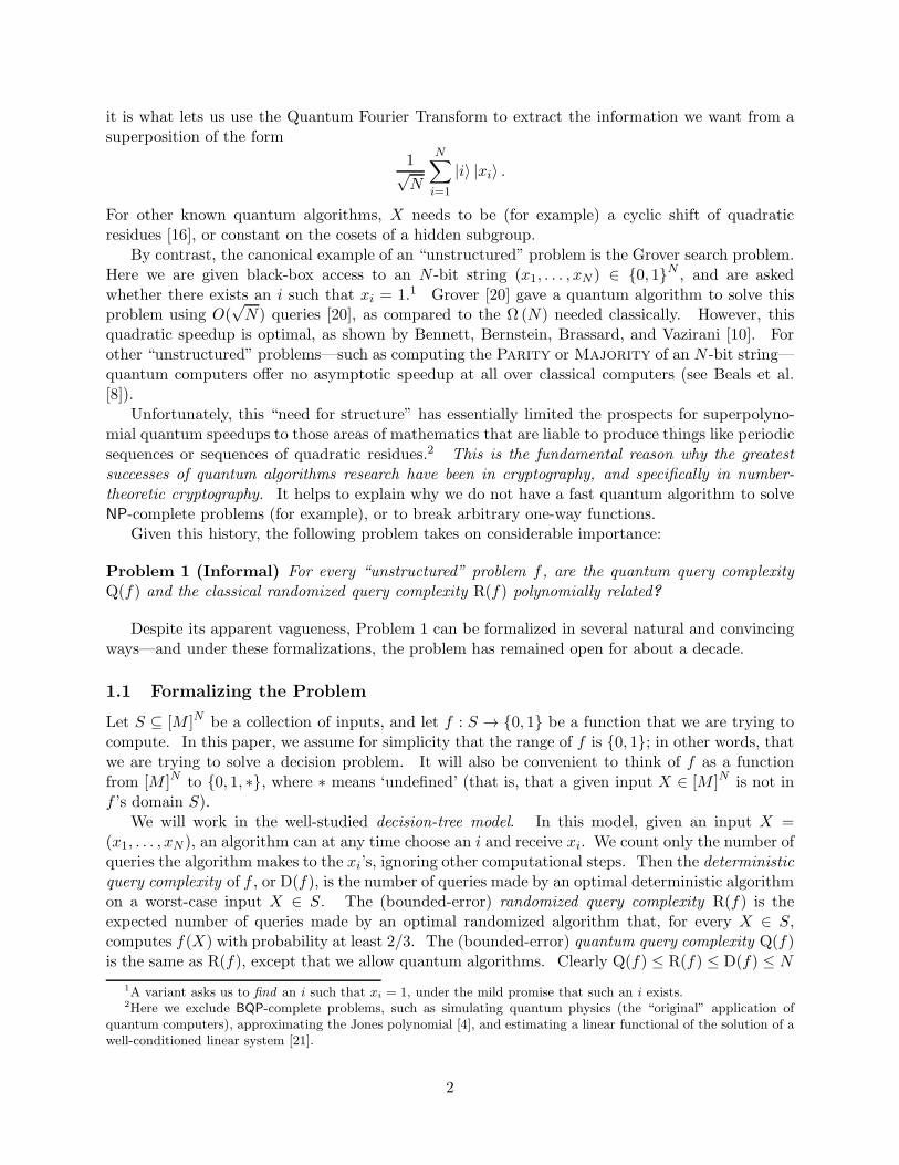
Let X = (x1, . . . , xN ) be an input. For each j ∈ [M ], let κj be the number of i’s such that xi = j.Then the first step is to give a classical randomized algorithm that estimates the κj ’s. Thisalgorithm, ST , is an extremely straightforward sampling procedure. (Indeed, there is essentiallynothing else that a randomized algorithm can do here.) ST will make O(T 1+c log T ) queries, whereT is a parameter and c ∈ (0, 1] is a constant that we will choose later to optimize the final bound.

Set U := 21T 1+c lnTChoose U indices i1, . . . , iU ∈ [N ] uniformly at random with replacement

8

Query xi1 , . . . , xiUFor each j ∈ [M ]:

Let zj be the number of occurrences of j in (xi1 , . . . , xiU )Output κj :=

zjU ·N as the estimate for κj

We now analyze how well ST works.

Lemma 11 With probability 1−O (1/T ), we have |κj − κj | ≤ NT +

κj

T c for all j ∈ [M ].

Proof. For each j ∈ [M ], we consider four cases. First suppose κj ≥ N/T 1−c. Notice that zj isa sum of U independent Boolean variables, and that E [zj ] =

UN E[κj ] =

UN κj . Thus

Pr[|κj − κj | >

κjT c

]= Pr

[∣∣∣∣zj −U

Nκj

∣∣∣∣ >UκjNT c

]

< 2 exp

(−Uκj/N

3T 2c

)

< 2 exp

(− U

3T 1+c

)

= 2T−7,

where the second line follows from a Chernoff bound and the third from κj ≥ N/T 1−c.Second, suppose N/T ≤ κj < N/T 1−c. Then

Pr

[|κj − κj | >

N

T

]= Pr

[∣∣∣∣zj −U

Nκj

∣∣∣∣ >U

T

]

< 2 exp

(−Uκj/N

3

(N

Tκj

)2)

< 2 exp

(− U

3T 1+c

)

= 2T−7

where the second line follows from a Chernoff bound (which is valid because NTκj

≤ 1) and the third

from κj < N/T 1−c.Third, suppose N/T 6 ≤ κj < N/T . Then

Pr

[|κj − κj | >

N

T

]= Pr

[∣∣∣∣zj −U

Nκj

∣∣∣∣ >U

T

]

<

(eN/(Tκj)

(1 +N/ (Tκj))1+N/(Tκj)

)Uκj/N

≤ exp

(− N

Tκj· Uκj

N

)

= exp

(−U

T

)

= O

(1

T 7

),

9

where the second line follows from a Chernoff bound, the third line follows from NTκj

> 1, and the

last follows from U = 21T 1+c lnT .Fourth, suppose κj < N/T 6. Then

Pr

[|κj − κj | >

N

T

]= Pr

[∣∣∣∣zj −U

Nκj

∣∣∣∣ >U

T

]

≤ Pr [zj ≥ 2]

≤(U

2

)(κjN

)2

≤ U2

T 6

(κjN

)

≤ κjTN

for all sufficiently large T , where the second line follows from κj < N/T 6, the third from the unionbound, the fourth from κj < N/T 6 (again), and the fifth from U ≤ 21T 2 lnT .

Notice that there are at most T 6 values of j such that κj ≥ N/T 6. Hence, putting all fourcases together,

Pr

[∃j : |κj − κj | >

N

T+

κjT c

]≤ T 6 · O

(1

T 7

)+

∑

j:κj<N/T 6

κjTN

= O

(1

T

).

Now call A a 1-type if f(X) = 1 for all X ∈ A, or a 0-type if f(X) = 0 for all X ∈ A. Considerthe following randomized algorithm RT to compute f(X):

Run ST to find an estimate κi for each κiSort the κi’s in descending order, so that κ1 ≥ · · · ≥ κMIf there exists a 1-type A = (a1, a2, . . .) such that |κi − ai| ≤ N

T + aiT c

for all i, then output f(X) = 1Otherwise output f(X) = 0

Clearly RT makes O(T 1+c log T ) queries, just as ST does. We now give a sufficient conditionfor RT to succeed.

Lemma 12 Suppose that for all 1-types A = (a1, a2, . . .) and 0-types B = (b1, b2, . . .), there existsan i such that |ai − bi| > 2N

T + ai+biT c . Then RT computes f with bounded probability of error, and

hence R(f) = O(T 1+c log T ).

Proof. First suppose X ∈ A where A = (a1, a2, . . .) is a 1-type. Then by Lemma 11, withprobability 1−O (1/T ) we have |κi − ai| ≤ N

T + aiT c for all i. (It is easy to see that sorting the κi’s

can only decrease the maximum difference.) Provided this occurs, RT finds some 1-type close to(κ1, κ2, . . .) (possibly A itself) and outputs f(X) = 1.

Second, suppose X ∈ B where B = (b1, b2, . . .) is a 0-type. Then with probability 1− O (1/T )we have |κi − bi| ≤ N

T + biT c for all i. Provided this occurs, by the triangle inequality, for every

1-type A = (a1, a2, . . .) there exists an i such that

|κi − ai| ≥ |ai − bi| − |κi − bi| >N

T+

aiT c

.

10

Hence RT does not find a 1-type close to (κ1, κ2, . . .), and it outputs f(X) = 0.In particular, suppose we keep decreasing T until there exists a 1-type A∗ = (a1, a2, . . .) and a

0-type B∗ = (b1, b2, . . .) such that

|ai − bi| ≤2N

T+

ai + biT c

(1)

for all i, stopping as soon as that happens. Then Lemma 12 implies that we will still haveR (f) = O(T 1+c log T ). For the rest of the proof, we will fix that “almost as small as possible”value of T for which (1) holds, as well as the 1-type A∗ and the 0-type B∗ that RT “just barelydistinguishes” from one another.

2.2 The Chopping Procedure

Given two sets of inputs A and B with A∩B = ∅, let Q(A,B) be the minimum number of queriesmade by any quantum algorithm that accepts every X ∈ A with probability at least 2/3, andaccepts every Y ∈ B with probability at most 1/3. Also, let Qε(A,B) be the minimum number ofqueries made by any quantum algorithm that accepts every X ∈ A with at least some probabilityp, and that accepts every Y ∈ B with probability at most p− ε. Then we have the following basicrelation:

Proposition 13 Q(A,B) = O(1ε Qε(A,B)) for all A,B and all ε > 0.

Proof. This follows from standard amplitude estimation techniques (see Brassard et al. [12] forexample).

The rest of the proof consists of lower-bounding Q(A∗,B∗), the quantum query complexity ofdistinguishing inputs of type A∗ from inputs of type B∗. We do this via a hybrid argument. LetL := ⌈log2 N⌉+ 1. At a high level, we will construct a sequence of types A0, . . . ,A2L such that

(i) A0 = A∗,

(ii) A2L = B∗, and

(iii) Q(Aℓ,Aℓ−1) is large for every ℓ ∈ [2L].

Provided we can do this, it is not hard to see that we get the desired lower bound on Q(A∗,B∗).Suppose a quantum algorithm distinguishes A0 = A∗ from A2L = B∗ with constant bias. Thenby the triangle inequality, it must also distinguish some Aℓ from Aℓ+1 with reasonably large bias(say Ω (1/ logN)). By Proposition 13, any quantum algorithm that succeeds with bias ε can beamplified, with O (1/ε) overhead, to an algorithm that succeeds with constant bias.

Incidentally, the need, in this hybrid argument, to amplify the distinguishing bias ε = εℓ fromΩ (1/ logN) to Ω (1) is exactly what could produce an undesired 1/ logN factor in our final lowerbound on Q(f), if we were not careful. (We mentioned this issue in Section 1.2.) The way we willsolve this problem, roughly speaking, is to design the Aℓ’s in such a way that our lower bounds onQ(Aℓ,Aℓ−1) increase quickly as functions of ℓ. That way, we can take the biases εℓ to decreasequadratically with ℓ (thus summing to a constant), yet still have Q(Aℓ,Aℓ−1) increasing quicklyenough that

Qεℓ(Aℓ,Aℓ−1) = Ω(εℓQ(Aℓ,Aℓ−1))

remain “uniformly large,” with 1/ log T factors but no 1/ logN factor.

11

Figure 1: Chopping a row of Aℓ’s Young diagram to make it more similar to Bℓ.

We now describe the procedure for creating the intermediate types Aℓ. Intuitively, we want toform Aℓ from Aℓ−1 by making its Young diagram more similar to that of B∗, by decreasing therows of Aℓ−1 which are larger than the corresponding rows of B∗ and increasing the rows of Aℓ−1

which are smaller than the corresponding rows of B∗.More precisely, we construct the intermediate types A1,A2, . . . via the following procedure. In

this procedure, (a1, a2, . . .) is an input type that is initialized to A∗, and B∗ = (b1, b2, . . .).

let P be the first power of 2 greater than or equal to Nfor ℓ := 1 to L

let SA be the set of i such that ai − bi ≥ P/2l

let SB be the set of i such that bi − ai ≥ P/2l

let m := min(|SA| , |SB|)choose m elements i from SA, set ai := ai −P/2ℓ and remove them from SA

choose m elements i from SB, set ai := ai+P/2ℓ and remove them from SB

let A2ℓ−1 := type(a1, a2, . . .)if |SA| > 0

let ai := ai − P/2ℓ for all i ∈ SA

choose |SA| elements i such that ai < bi and set ai := ai + P/2ℓ

if |SB | > 0let ai := ai + P/2ℓ for all i ∈ SB

choose |SB| elements i such that ai > bi and set ai := ai − P/2ℓ

let A2ℓ := type(a1, a2, . . .)next ℓ

The procedure is illustrated pictorially in Figure 1.We start with some simple observations. First, by construction, this procedure halts after

2L = O (logN) iterations. Second, after the ℓth iteration, we have |ai − bi| < P2ℓ

for all i. This

follows by induction. Let a′i be the value of ai before the ℓth iteration. Because of the inductiveassumption, we must have |a′i − bi| < P

2ℓ−1—for if |a′i − bi| ≥ P2ℓ, then ai is changed by P

2ℓduring

the ℓth iteration, to decrease the difference |ai − bi|. After this change,

|ai − bi| =∣∣a′i − bi

∣∣− P

2ℓ<

P

2ℓ−1− P

2ℓ=

P

2ℓ.

Besides the |a′i − bi| ≥ P2ℓ

case, there is one other case where |ai − bi| could change. In the transitionfrom A2ℓ−1 to A2ℓ, if |SA| > 0 or |SB| > 0, then we change ai for |SA| or |SB| elements i that do notbelong to SA or SB . For those elements, we have |ai − bi| < P

2ℓand we change ai in the direction

12

of bi (we increase it by P2ℓ

if ai < bi and decrease it by the same amount if ai > bi). Therefore,

after the change, the sign of the difference ai − bi flips and |ai − bi| < P2ℓ.

Now let us define

‖A − B‖ :=1

2

N∑

i=1

|ai − bi| .

Notice that ‖Aℓ −Aℓ−1‖ = rP/2ℓ′, where r is the number of rows that get increased (or decreased)

in the ℓth iteration and l′ = ⌈ l2⌉. We now prove an upper bound on ‖Aℓ −Aℓ−1‖ when ℓ is small,

which will be useful later.

Lemma 14 If ℓ ≤ (log2 T )− 2, then

‖A2ℓ−2 −A2ℓ−1‖+ ‖A2ℓ−1 −A2ℓ‖ ≤ 4N

T c.

Proof. Let m := max(|SA| , |SB |). Then

‖A2ℓ−2 −A2ℓ−1‖+ ‖A2ℓ−1 −A2ℓ‖ = mP

2ℓ.

Without loss of generality, we assume that m = |SA|. To show the lemma, it suffices to prove that

|SA| ≤ 4N/T c

P/2ℓ.

We consider the sum∑

j∈R |aj − bj| where R is the set of all j such that |aj − bj| ≥ P2ℓ, with

(a1, a2, . . .) evolving from A0 to A2ℓ−2 and B∗ = (b1, b2, . . .) fixed. Initially (when (a1, a2, . . .) =A0), we have

P

2ℓ≤ |aj − bj| ≤

2N

T+

aj + bjT c

for each j ∈ R. Since ℓ ≤ (log2 T )− 2, the left inequality implies

|aj − bj| ≥4N

T,

which combined with the right inequality yields

aj + bjT c

≥ 2N

T. (2)

Therefore

∑

i∈R|ai − bi| ≤

∑

i∈R

(2N

T+

ai + biT c

)

≤ 2∑

i∈R

ai + biT c

≤ 4N

T c,

where the third line uses (2).The sum

∑i∈R |ai − bi| is not increased by any step of the algorithm that generates A0, . . . ,A2ℓ−2.

Therefore, at the beginning of the ℓth iteration, we still have∑

i∈R |ai − bi| ≤ 4NT c . This means that

|SA| ≤ 4N/T c

P/2ℓ.

13

2.3 Quantum Lower Bounds

Recall that we listed four properties that we needed the chopping procedure to satisfy. We havealready seen that it satisfies properties (i)-(ii), so the remaining step is to show that it satisfiesproperty (iii). That is, we need to lower-bound Q(Aℓ,Aℓ−1), the bounded-error quantum querycomplexity of distinguishing inputs of type Aℓ from inputs of type Aℓ−1. To do this, it will beconvenient to consider two cases: first, that forming Aℓ involved chopping few elements of Aℓ−1,and second, that it involved chopping many elements. We will show that we “win either way,” bya different quantum lower bound in each case.

First consider the case that few elements were chopped. Here we prove a lower bound usingAmbainis’s quantum adversary method [5], in its “general” form (the one used, for example, tolower-bound the quantum query complexity of inverting a permutation). For completeness, wenow state Ambainis’s adversary theorem in the form we will need.

Theorem 15 (Ambainis [5]) Let A,B ⊆ [M ]N be two sets of inputs with A ∩ B = ∅. LetR ⊆ A×B be a relation on input pairs, such that for every X ∈ A there exists at least one Y ∈ Bwith (X,Y ) ∈ R and vice versa. Given inputs X = (x1, . . . , xN ) in A and Y = (y1, . . . , yN ) in B,let

qX,i = PrY ∈B

[xi 6= yi | (X,Y ) ∈ R] ,

qY,i = PrX∈A

[xi 6= yi | (X,Y ) ∈ R] .

Suppose that qX,iqy,i ≤ α for every (X,Y ) ∈ R and every i ∈ [N ] such that xi 6= yi. ThenQ(A,B) = Ω(1/

√α).

Using Theorem 15, we can prove the following lower bound on Q (Aℓ,Aℓ−1).

Lemma 16 Let d = ‖Aℓ −Aℓ−1‖, and assume d ≤ N/2. Then Q(Aℓ,Aℓ−1) = Ω(√

N/d).

Proof. Let Aℓ−1 = (a1, a2, . . .), and let ℓ′ = ⌈ ℓ2⌉. Then in the transition from Aℓ−1 to Aℓ, we

augment or chop various rows by P/2ℓ′elements each. Let i (1) , . . . , i (r) be the r rows in Aℓ−1

that get chopped and let i′ (1) , . . . , i′ (r) be the r rows in Aℓ−1 that get augmented.Fix distinct h1, . . . , hr ∈ [M ] and h′1, . . . , h

′r ∈ [M ]. Also, let us restrict ourselves to inputs

such that for each j ∈ [r], there are exactly ai(j) indices i ∈ [N ] satisfying xi = hj and exactly ai′(j)indices i ∈ [N ] satisfying xi = h′j . G iven inputs X = (x1, . . . , xN ) in Aℓ−1 and Y = (y1, . . . , yN )in Aℓ, we set (X,Y ) ∈ R if and only if it is possible to transform X to Y in the following way:

(1) For each j ∈ [r], change exactly P/2ℓ′of the xi’s that are equal to hj to value h′j . (The total

number of changed elements is d.)

(2) Swap the d elements of X that were changed in step (2) with any other d elements xi of X,subject to the following constraints:

(a) we do not use xi such that xi = hj for some j andaij−P/2ℓ

′

P/2ℓ′< N−d

3d ;

(b) we do not use xi such that xi = h′j for some j andaij

P/2ℓ′< N−d

3d .

The procedure is illustrated pictorially in Figure 2. Note that we can reverse the procedure ina natural way to go from Y back to X:

14

Figure 2: In this example, N = 11, r = 2, P/2ℓ = 2, and a1 = a2 = 3. So we transform X to Y bychoosing h1 = 1 and h2 = 2, changing any two elements equal to h1 and any two elements equal toh2, and then swapping the four elements that we changed with four unchanged elements.

(1) For each j ∈ [r], change exactly P/2ℓ′of the xi’s that are equal to h′j to value hj .

(2) Swap the d elements of X that were changed in step (2) with any d elements xi of X, subjectto the same constraints as in the step (2) of the X → Y conversion.

Fix any (X,Y ) ∈ R, and let i ∈ [N ] be any index such that xi 6= yi. Then we claim thatthe parameters of Theorem 15 satisfy either qX,i ≤ 6d

N−d or qY,i ≤ 6dN−d . To see this, let us write

qX,i = q′X,i + q′′X,i, where q′X,i is the probability that xi is changed in step (1) of the X → Yconversion and q′′X,i is the probability that xi is not changed in step (1), but is swapped with somechanged element in step (2). We also express qY,i in a similar way, with respect to the Y → Xconversion.

We consider two cases. The first case is that xi is one of the “other d elements” with whichwe swap the changed elements in step (2) of the X → Y conversion. In this case, q′X,i 6= 0 only if

xi = hj for some j. Then because of the constraint (a), we have q′X,i ≤ 3dN+2d . We also have

q′′X,i = PrY ′∈Aℓ

[xi 6= y′i |

(X,Y ′) ∈ R

]≤ d

(N − d)/3=

3d

N − d,

because each of the constraints (a) and (b) eliminates at most (N − d)/3 of the N − d variables xithat are available for swapping in step (2). Therefore, qX,i = q′X,i + q′′X,i ≤ 6d

N−d .The second case is that xi is one of the elements that are changed in step (1) of the X → Y

conversion. Then yi is one of the “other d elements” in step (2) of the Y → X conversion. Similarlyto the previous case, we can show that qY,i ≤ 6d

N−d .Since qX,i ≤ 1 and qY,i ≤ 1, it follows that

qX,iqY,i ≤6d

N − d.

Thus, by Theorem 15,

Q(Aℓ,Aℓ−1) = Ω

(1

√qX,iqY,i

)= Ω

(√N − d

d

)= Ω

(√N

d

).

We now consider the case that many elements are chopped. Here we prove a lower bound byreduction from SetEquality. Given two sequences of integers Y ∈ [M ]N and Z ∈ [M ]N , neitherwith any repeats, the SetEquality problem is to decide whether Y and Z are equal as sets ordisjoint as sets, promised that one of these is the case. SetEquality is similar to the collision

15

problem studied by Aaronson and Shi [3], but it lacks permutation symmetry, making it harderto prove a lower bound by the polynomial method. By combining the collision lower bound withAmbainis’s adversary method, Midrijanis [24] was nevertheless able to show that

Q (SetEquality) = Ω

((N

logN

)1/5).

Very recently, and using different ideas, Zhandry [33] managed to improve Midrijanis’s lower boundto the following:

Theorem 17 (Zhandry [33]) Q(SetEquality) = Ω(N1/3).

Theorem 17 is known to be tight, by the upper bound of Brassard, Høyer, and Tapp [13]mentioned in Section 1.1.

We will consider a modification of the SetEquality problem, which we call 3SetEquality.Here we are given three sequences of integers Y,Z,W ∈ [M ]N , none of which has any repeats. Weare promised that Y and W are disjoint as sets, and that Z is equal either to Y or to W as a set.The task is to distinguish between those two cases.

Theorem 18 Q(3SetEquality) = Ω(N1/3).

Proof. The theorem follows from Theorem 17 together with the following claim: if 3SetEqualityis solvable by a quantum algorithm A that uses T queries, then 3SetEquality is solvable by aquantum algorithm that uses O(T ) queries.

To show this, let Y,W be an instance of SetEquality. We produce an instance of 3SetE-quality by choosing Z to be either a randomly permuted version of Y or a randomly permutedversion of W . We then run the algorithm for 3SetEquality on that instance. If Y and W aredisjoint, then the promise of 3SetEquality is satisfied and the algorithm will find whether weused Y or W to generate Z. If Y = W , then using Y and using W results in the same proba-bility distribution for Z; hence no algorithm will be able to guess whether we used Y or W withprobability greater than 1/2.

We now use Theorem 18 to prove another lower bound on Q(Aℓ,Aℓ−1).

Lemma 19 Suppose Aℓ was formed from Aℓ−1 by chopping r rows. Then Q(Aℓ,Aℓ−1) = Ω(r1/3

).

Proof. We will show how to embed a 3SetEquality instance of size r into the Aℓ versus Aℓ−1

problem.Let Aℓ−1 = (a1, . . . , au). Also, let i (1) , . . . , i (r) ∈ [u] be the r rows that are chopped in

going from Aℓ−1 to Aℓ, let i′ (1) , . . . , i′ (r) ∈ [u] be the r rows that are augmented, and letj (1) , . . . , j (u− 2r) ∈ [u] be the u − 2r rows that are left unchanged. Recall that, in goingfrom Aℓ−1 to Aℓ, each row i (k) (or i′ (k)) is chopped or augmented by P/2ℓ

′elements, where

ℓ′ = ⌈ ℓ2⌉.

Now let Y = (y1, . . . , yr), Z = (z1, . . . , zr), W = (z1, . . . , zr) be an instance of 3SetEquality.Then we construct an input X ∈ [M ]N as follows. First, for each k ∈ [r], set ai(k) − P/2ℓ

′of the

xi’s equal to yk, set P/2ℓ′of the xi’s equal to zk and set a′i(k) of the xi’s equal to wk. Next, let

w1, w2, . . . ∈ [M ] be a list of numbers that are guaranteed not to be in Y ∪ Z. Then for eachk ∈ [u− 2r], set aj(k) of the xi’s equal to wk.

It is easy to see that, if Y and Z are equal as sets, then X will have type Aℓ−1, while if Z andW are equal as sets, then X will have type Aℓ. So in deciding whether X belongs to Aℓ or Aℓ−1,we also decide whether Y = Z or Z = W . The lemma now follows from Theorem 18.

16

2.4 Putting Everything Together

Let C be a quantum query algorithm that distinguishes A0 = A∗ from A2L = B∗, and assume C isoptimal: that is, it makes Q(A∗,B∗) ≤ Q(f) queries. As mentioned earlier, we can assume thatPr [C accepts X] depends only on the type of X. Thus, let

pℓ := Pr [C accepts X ∈ Aℓ] .

Then by assumption, |p0 − p2L| ≥ 1/3. Now let βℓ := 110ℓ2

, and observe that∑∞

ℓ=1 βℓ < 16 . By

the triangle inequality, it follows that there exists an ℓ ∈ [2L] such that |pℓ − pℓ−1| ≥ βℓ. In otherwords, we get a Q(f)-query quantum algorithm that distinguishes Aℓ from Aℓ−1 with bias βℓ. ByProposition 13, this immediately implies

Q(Aℓ,Aℓ−1) = O

(Q(f)

βℓ

)

or equivalently

Q(f) = Ω

(Q(Aℓ,Aℓ−1)

ℓ2

).

Now let d = ‖Aℓ −Aℓ−1‖, and suppose Aℓ was produced from Aℓ−1 by chopping r rows. Thend = rP/2ℓ

′ ≤ 2rN/2ℓ′where l′ = ⌈ l

2⌉. Combining Lemmas 16 and 19, we find that

Q(Aℓ,Aℓ−1) = Ω

(max

√N

d, r1/3

)

= Ω

(√2ℓ′

r+ r1/3

)

= Ω(2ℓ

′/5),

since the minimum occurs when r is asymptotically 23ℓ′/5. If ℓ′ ≤ (log2 T ) − 2, then combining

Lemmas 16 and 14, we also have the lower bound

Q(Aℓ,Aℓ−1) = Ω

(√N

4N/T c

)= Ω(

√T c).

Hence

Q(f) =

Ω(√

T c

ℓ2

)if ℓ′ ≤ (log2 T )− 2

Ω(2ℓ

′/5)

if ℓ′ > (log2 T )− 2.

Let us now make the choice c = 2/5, so that we get a lower bound of

Q(f) = Ω

(T 1/5

log2 T

)

in either case. Hence T = O(Q(f)5 log10 Q(f)). By Lemma 12:

R(f) = O(T 1+c log T )

= O(T 7/5 log T )

= O(Q(f)7 log15 Q(f)).

This completes the proof of Theorem 5.

17

3 Quantum Lower Bounds Under The Uniform Distribution

In this section, we consider the problems of P?= BQP relative to a random oracle, and of simulating

a T -query quantum algorithm on most inputs using TO(1) classical queries. We show that theseproblems are connected to a fundamental conjecture about influences in low-degree polynomials.

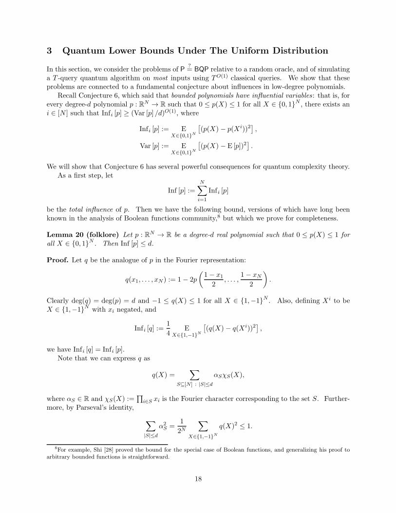
Recall Conjecture 6, which said that bounded polynomials have influential variables: that is, forevery degree-d polynomial p : RN → R such that 0 ≤ p(X) ≤ 1 for all X ∈ 0, 1N , there exists ani ∈ [N ] such that Infi [p] ≥ (Var [p] /d)O(1), where

Infi [p] := EX∈0,1N

[(p(X) − p(Xi))2

],

Var [p] := EX∈0,1N

[(p(X) − E [p])2

].

We will show that Conjecture 6 has several powerful consequences for quantum complexity theory.As a first step, let

Inf [p] :=

N∑

i=1

Inf i [p]

be the total influence of p. Then we have the following bound, versions of which have long beenknown in the analysis of Boolean functions community,8 but which we prove for completeness.

Lemma 20 (folklore) Let p : RN → R be a degree-d real polynomial such that 0 ≤ p(X) ≤ 1 forall X ∈ 0, 1N . Then Inf [p] ≤ d.

Proof. Let q be the analogue of p in the Fourier representation:

q(x1, . . . , xN ) := 1− 2p

(1− x1

2, . . . ,

1− xN2

).

Clearly deg(q) = deg(p) = d and −1 ≤ q(X) ≤ 1 for all X ∈ 1,−1N . Also, defining Xi to beX ∈ 1,−1N with xi negated, and

Inf i [q] :=1

4E

X∈1,−1N[(q(X)− q(Xi))2

],

we have Inf i [q] = Infi [p].Note that we can express q as

q(X) =∑

S⊆[N ] : |S|≤d

αSχS(X),

where αS ∈ R and χS(X) :=∏

i∈S xi is the Fourier character corresponding to the set S. Further-more, by Parseval’s identity,

∑

|S|≤d

α2S =

1

2N

∑

X∈1,−1Nq(X)2 ≤ 1.

8For example, Shi [28] proved the bound for the special case of Boolean functions, and generalizing his proof toarbitrary bounded functions is straightforward.

18

Now, in the Fourier representation, it is known that

Inf i [q] =∑

|S|≤d : i∈Sα2S .

Hence

Inf [p] = Inf [q] =∑

i∈[N ]

∑

|S|≤d : i∈Sα2S =

∑

|S|≤d

∑

i∈Sα2S =

∑

|S|≤d

|S|α2S ≤ d

∑

|S|≤d

α2S ≤ d

as claimed.We also need the following lemma of Beals et al. [8].

Lemma 21 (Beals et al.) Suppose a quantum algorithm Q makes T queries to a Boolean inputX ∈ 0, 1N . Then Q’s acceptance probability is a real multilinear polynomial p(X), of degree atmost 2T .

3.1 Consequences of Our Influence Conjecture

We now prove our first consequence of Conjecture 6: namely, that it implies the folklore Conjecture4.

Theorem 22 Suppose Conjecture 6 holds, and let ε, δ > 0. Then given any quantum algorithmQ that makes T queries to a Boolean input X, there exists a deterministic classical algorithmthat makes poly(T, 1/ε, 1/δ) queries, and that approximates Q’s acceptance probability to within anadditive constant ε on a 1− δ fraction of inputs.

Proof. Let p(X) be the probability that Q accepts input X = (x1, . . . , xN ). Then Lemma 21 saysthat p is a real polynomial of degree at most 2T . Assume Conjecture 6. Then for every suchp, there exists an index i satisfying Infi [p] ≥ w(Var [p] /T ), for some fixed polynomial w. Underthat assumption, we give a classical algorithm C that makes poly(T, 1/ε, 1/δ) queries to the xi’s,and that approximates p(X) on most inputs X. In what follows, assume X ∈ 0, 1N is uniformlyrandom.

set p0 := pfor j := 0, 1, 2, . . .:

if Var [pj] ≤ ε2δ/2output EY ∈0,1N−j [pj(Y )] as approximation for p(X) and halt

else

find an i ∈ [N − j] such that Infi [pj] > w(ε2δ/2T )query xi, and let pj+1 : R

N−j → R be the polynomial

induced by the answer

When C halts, by assumption Var [pj] ≤ ε2δ/2. By Markov’s inequality, this implies

PrX∈0,1N−j

[|pj(X) − E [pj]| > ε] <δ

2,

meaning that when C halts, it succeeds with probability at least 1− δ/2.

19

On the other hand, suppose Var [pj ] > ε2δ/2. Then by Conjecture 6, there exists an indexi∗ ∈ [N ] such that

Inf i∗ [pj] ≥ w

(Var [pj ]

T

)≥ w

(ε2δ

2T

).

Thus, suppose we query xi∗ . Since X is uniformly random, xi∗ will be 0 or 1 with equal probability,even conditioned on the results of all previous queries. So after the query, our new polynomialpj+1 will satisfy

Pr[pj+1 = pj|xi∗=0

]= Pr

[pj+1 = pj|xi∗=1

]=

1

2,

where pj|xi∗=0 and pj|xi∗=1 are the polynomials on N−j−1 variables obtained from pj by restrictingxi∗ to 0 or 1 respectively. Therefore

Exi∗∈0,1

[Inf [pj+1]] =1

2

(Inf[pj|xi∗=0

]+ Inf

[pj|xi∗=1

])

=1

2

∑

i 6=i∗

Infi[pj|xi∗=0

]+∑

i 6=i∗

Inf i[pj|xi∗=1

]

=∑

i 6=i∗

Infi [pj]

= Inf [pj ]− Infi∗ [pj]

≤ Inf [pj ]− w

(ε2δ

2T

).

By linearity of expectation, this imples that for all j,

EX∈0,1N

[Inf [pj ]] ≤ Inf [p0]− jw

(ε2δ

2T

)

But recall from Lemma 20 thatInf [p0] ≤ deg (p0) ≤ 2T.

It follows that C halts after an expected number of iterations that is at most

Inf [p0]

w(ε2δ/2T )≤ 2T

w(ε2δ/2T ).

Thus, by Markov’s inequality, the probability (over X) that C has not halted after 4Tδ·w(ε2δ/2T )

iterations is at most δ/2. Hence by the union bound, the probability over X that C fails is at mostδ/2 + δ/2 = δ. Since each iteration queries exactly one variable and

4T

δ · w(ε2δ/2T ) = poly(T, 1/ε, 1/δ),

this completes the proof.An immediate corollary is the following:

Corollary 23 Suppose Conjecture 6 holds. Then Dε+δ(f) ≤ (Qε(f)/δ)O(1) for all Boolean func-

tions f and all ε, δ > 0.

20

Proof. Let Q be a quantum algorithm that evaluates f(X), with bounded error, on a 1−ε fractionof inputs X ∈ 0, 1N . Let p(X) := Pr [Q accepts X]. Now run the classical simulation algorithmC from Theorem 22, to obtain an estimate p(X) of p(X) such that

PrX∈0,1N

[|p(X) − p(X)| ≤ 1

10

]≥ 1− δ.

Output f(X) = 1 if p(X) ≥ 12 and f(X) = 0 otherwise. By the theorem, this requires poly(T, 1/δ)

queries to X, and by the union bound it successfully computes f(X) on at least a 1− ε− δ fractionof inputs X.

We also get the following complexity-theoretic consequence:

Theorem 24 Suppose Conjecture 6 holds. Then P = P#P implies BQPA ⊂ AvgPA with proba-bility 1 for a random oracle A.

Proof. Let Q be a polynomial-time quantum Turing machine that queries an oracle A, andassume Q decides some language L ∈ BQPA with bounded error. Given an input x ∈ 0, 1n, letpx(A) := Pr

[QA(x) accepts

]. Then clearly px(A) depends only on some finite prefix B of A, of

size N = 2poly(n). Furthermore, Lemma 21 implies that px is a polynomial in the bits of B, ofdegree at most poly(n).

Assume Conjecture 6 as well as P = P#P. Then we claim that there exists a deterministicpolynomial-time algorithm C such that for all Q and x ∈ 0, 1n,

PrA

[|px(A)− px(A)| >

1

10

]<

1

n3, (3)

where px(A) is the output of C given input x and oracle A. This C is essentially just the algorithmfrom Theorem 22. The key point is that we can implement C using not only poly(n) queries toA, but also poly(n) computation steps.

To prove the claim, let M be any of the 2poly(n) monomials in the polynomial pj from Theorem22, and let αM be the coefficient of M . Then notice that αM can be computed to poly(n) bits ofprecision in P#P, by the same techniques used to show BQP ⊆ P#P [11]. Therefore the expectation

EY ∈0,1N−j

[pj(Y )] =∑

M

αM

2|M |

can be computed in P#P as well. The other two quantities that arise in the algorithm—Var [pj ]and Infi [pj]—can also be computed in P#P, since they are simply sums of squares of differences ofpj(X)’s. This means that finding an i such that Infi [pj] > w(ε2δ/T ) is in NP#P. But under theassumption that P = P#P, we have P = NP#P as well. Therefore all of the computations neededto implement C take polynomial time.

Now let δn(A) be the fraction of inputs x ∈ 0, 1n such that |px(A)− px(A)| > 110 . Then by

(3) together with Markov’s inequality,

PrA

[δn(A) >

1

n

]<

1

n2.

Since∑∞

n=11n2 converges, it follows that δn(A) ≤ 1

n for all but finitely many values of n, withprobability 1 over A. Assuming this occurs, we can simply hardwire the behavior of Q on theremaining n’s into our classical simulation procedure C. Hence L ∈ AvgPA.

21

Since the number of BQPA languages is countable, the above implies that L ∈ AvgPA for everyL ∈ BQPA simultaneously (that is, BQPA ⊂ AvgPA) with probability 1 over A.

As a side note, suppose we had an extremely strong variant of Conjecture 6, one that impliedsomething like

PrA

[|px(A)− px(A)| >

1

10

]<

1

exp(n).

in place of (3). Then we could eliminate the need for AvgP in Theorem 24, and show that P = P#P

implies PA = BQPA with probability 1 for a random oracle A.

3.2 Unconditional Results

We conclude this section with some unconditional results. These results will use Theorem 9 ofDinur et al. [18]: that for every degree-d polynomial p : RN → R such that 0 ≤ p(X) ≤ 1 forall X ∈ 0, 1N , there exists a polynomial p depending on at most 2O(d)/ε2 variables such that‖p− p‖22 ≤ ε, where

‖p‖22 := EX∈0,1N

[p(X)2

].

Theorem 9 has the following simple corollary.

Corollary 25 Suppose a quantum algorithm Q makes T queries to a Boolean input X ∈ 0, 1N .Then for all α, δ > 0, we can approximate Q’s acceptance probability to within an additive constant

α, on a 1− δ fraction of inputs, by making 2O(T )

α4δ4deterministic classical queries to X. (Indeed, the

classical queries are nonadaptive.)

Proof. Let p(X) := Pr [Q accepts X]. Then p is a degree-2T real polynomial by Lemma 21.

Hence, by Theorem 9, there exists a polynomial p, depending on K = 2O(T )

α4δ4variables xi1 , . . . , xiK ,

such thatE

X∈0,1N[(p(X)− p(X))2

]≤ α2δ2.

By the Cauchy-Schwarz inequality, then,

EX∈0,1N

[|p(X) − p(X)|] ≤ αδ,

so by Markov’s inequalityPr

X∈0,1N[|p(X)− p(X)| > α] < δ.

Thus, our algorithm is simply to query xi1 , . . . , xiK , and then output p(X) as our estimate for p(X).

Likewise:

Corollary 26 Dε+δ(f) ≤ 2O(Qε(f))/δ4 for all Boolean functions f and all ε, δ > 0.

Proof. Set α to any constant less than 1/6, then use the algorithm of Corollary 25 to simulate theε-approximate quantum algorithm for f . Output f(X) = 1 if p(X) ≥ 1

2 and f(X) = 0 otherwise.

Given an oracle A, let BQPA[log] be the class of languages decidable by a BQP machine able tomake O (log n) queries to A. Also, let AvgPA

|| be the class of languages decidable, with probability

1 − o (1) over x ∈ 0, 1n, by a P machine able to make poly(n) parallel (nonadaptive) queries toA. Then we get the following unconditional variant of Theorem 24.

22

Theorem 27 Suppose P = P#P. Then BQPA[log] ⊂ AvgPA|| with probability 1 for a random oracle

A.

Proof. The proof is essentially the same as that of Theorem 24, except that we use Corollary 25in place of Conjecture 6. In the proof of Corollary 25, observe that the condition

EX∈0,1N

[|p(X) − p(X)|] ≤ αδ

impliesE

X∈0,1N[|pµ(X)− p(X)|] ≤ αδ (4)

as well, where pµ(X) equals the mean of p(Y ) over all inputs Y that agree with X on xi1 , . . . , xiK .Thus, given a quantum algorithm that makes T queries to an oracle string, the computationalproblem that we need to solve boils down to finding a subset of the oracle bits xi1 , . . . , xiK such

that K = 2O(T )

α4δ4and (4) holds. Just like in Theorem 24, this problem is solvable in the counting

hierarchy CH = P#P ∪ P#P#P ∪ · · · . So if we assume P = P#P, then it is also solvable in P.

In Theorem 24, the conclusion we got was BQPA ⊂ AvgPA with probability 1 for a randomoracle A. In our case, the number of classical queries K is exponential (rather than polynomial)in the number of quantum queries T , so we only get BQPA[log] ⊂ AvgPA. On the other hand, sincethe classical queries are nonadaptive, we can strengthen the conclusion to BQPA[log] ⊂ AvgPA

|| .

4 Open Problems

It would be nice to improve the R(f) = O(Q(f)7 polylogQ(f)) bound for all symmetric problems.As mentioned earlier, we conjecture that the right answer is R(f) = O(Q(f)2). In trying toimprove our lower bound, it seems best to avoid the use of SetEquality. After all, it is a curiousfeature of our proof that, to get a lower bound for symmetric problems, we need to reduce fromthe non-symmetric SetEquality problem!

Another problem is to remove the assumption M ≥ N in our lower bound for symmetricproblems. Experience with related problems strongly suggests that this can be done, but onemight need to replace our chopping procedure by something different.

We also conjecture that R(f) ≤ Q(f)O(1) for all partial functions f that are symmetric onlyunder permuting the inputs (and not necessarily the outputs). Proving this seems to require anew approach. Another problem, in a similar spirit, is whether R(f) ≤ Q(f)O(1) for all partialfunctions f : S → 0, 1 such that S (i.e., the promise on inputs) is symmetric, but f itself neednot be symmetric.

It would be interesting to reprove the R(f) ≤ Q(f)O(1) bound using only the polynomialmethod, and not the adversary method. Or, to rephrase this as a purely classical question: for allX = (x1, . . . , xN ) in [M ]N , let BX be the N ×M matrix whose (i, j)th entry is 1 if xi = j and 0

otherwise. Then given a set S ⊆ [M ]N and a function f : S → 0, 1, let deg(f) be the minimumdegree of a real polynomial p : RMN → R such that

(i) 0 ≤ p(BX) ≤ 1 for all X ∈ [M ]N , and

(ii) |p(BX)− f(X)| ≤ 13 for all X ∈ S.

23

Then is it the case that R(f) ≤ deg(f)O(1) for all permutation-invariant functions f?On the random oracle side, the obvious problem is to prove Conjecture 6—thereby establishing

that Dε(f) and Qδ(f) are polynomially related, and all the other consequences shown in Section3. Alternatively, one could look for some technique that was tailored to polynomials p that ariseas the acceptance probabilities of quantum algorithms. In this way, one could conceivably solveDε(f) versus Qδ(f) and the other quantum problems, without settling the general conjecture aboutbounded polynomials.

5 Acknowledgments

We thank Aleksandrs Belovs, Andy Drucker, Ryan O’Donnell, and Ronald de Wolf for helpful dis-cussions; Mark Zhandry for taking up our challenge to improve the lower bound on Q (SetEquality)to the optimal Ω(N1/3); and Dana Moshkovitz for suggesting a proof of Lemma 34. We especiallythank Arturs Backurs, Janis Iraids, the attendees of the quantum computing reading group at theUniversity of Latvia, and the anonymous reviewers for their feedback, and for catching some errorsin earlier versions of this paper.

References

[1] S. Aaronson. Quantum lower bound for the collision problem. In Proc. ACM STOC, pages635–642, 2002. quant-ph/0111102.

[2] S. Aaronson. BQP and the polynomial hierarchy. In Proc. ACM STOC, 2010. arXiv:0910.4698.

[3] S. Aaronson and Y. Shi. Quantum lower bounds for the collision and the element distinctnessproblems. J. ACM, 51(4):595–605, 2004.

[4] D. Aharonov, V. Jones, and Z. Landau. A polynomial quantum algorithm for approximatingthe Jones polynomial. In Proc. ACM STOC, pages 427–436, 2006. quant-ph/0511096.

[5] A. Ambainis. Quantum lower bounds by quantum arguments. J. Comput. Sys. Sci., 64:750–767, 2002. Earlier version in ACM STOC 2000. quant-ph/0002066.

[6] A. Ambainis and R. de Wolf. Average-case quantum query complexity. In Proc. Intl. Symp. onTheoretical Aspects of Computer Science (STACS), pages 133–144, 2000. quant-ph/9904079.

[7] A. Backurs and M. Bavarian. On the sum of L1 influences. arXiv:1302.4625, ECCC TR13-039,2013.

[8] R. Beals, H. Buhrman, R. Cleve, M. Mosca, and R. de Wolf. Quantum lower bounds bypolynomials. J. ACM, 48(4):778–797, 2001. Earlier version in IEEE FOCS 1998, pp. 352-361.quant-ph/9802049.

[9] J. N. de Beaudrap, R. Cleve, and J. Watrous. Sharp quantum versus classical query complexityseparations. Algorithmica, 34(4):449–461, 2002. quant-ph/0011065.

[10] C. Bennett, E. Bernstein, G. Brassard, and U. Vazirani. Strengths and weaknesses of quantumcomputing. SIAM J. Comput., 26(5):1510–1523, 1997. quant-ph/9701001.

24

[11] E. Bernstein and U. Vazirani. Quantum complexity theory. SIAM J. Comput., 26(5):1411–1473, 1997. First appeared in ACM STOC 1993.

[12] G. Brassard, P. Høyer, M. Mosca, and A. Tapp. Quantum amplitude amplification and estima-tion. In S. J. Lomonaco and H. E. Brandt, editors, Quantum Computation and Information,Contemporary Mathematics Series. AMS, 2002. quant-ph/0005055.

[13] G. Brassard, P. Høyer, and A. Tapp. Quantum algorithm for the collision problem. ACMSIGACT News, 28:14–19, 1997. quant-ph/9705002.

[14] H. Buhrman, L. Fortnow, I. Newman, and H. Rohrig. Quantum property testing. SIAM J.Comput., 37(5):1387–1400, 2008. Previous version in SODA’2003. quant-ph/0201117.

[15] H. Buhrman and R. de Wolf. Complexity measures and decision tree complexity: a survey.Theoretical Comput. Sci., 288:21–43, 2002.

[16] W. van Dam, S. Hallgren, and L. Ip. Quantum algorithms for some hidden shift problems.SIAM J. Comput., 36(3):763–778, 2006. Conference version in SODA 2003. quant-ph/0211140.

[17] D. Deutsch and R. Jozsa. Rapid solution of problems by quantum computation. Proc. Roy.Soc. London, A439:553–558, 1992.

[18] I. Dinur, E. Friedgut, G. Kindler, and R. O’Donnell. On the Fourier tails of bounded functionsover the discrete cube. In Proc. ACM STOC, pages 437–446, 2006.

[19] L. Fortnow and J. Rogers. Complexity limitations on quantum computation. J. Comput. Sys.Sci., 59(2):240–252, 1999. cs.CC/9811023.

[20] L. K. Grover. A fast quantum mechanical algorithm for database search. In Proc. ACM STOC,pages 212–219, 1996. quant-ph/9605043.

[21] A. Harrow, A. Hassidim, and S. Lloyd. Quantum algorithm for solving linear systems ofequations. Phys. Rev. Lett., 15(150502), 2009. arXiv:0811.3171.

[22] E. Hemaspaandra, L. A. Hemaspaandra, and M. Zimand. Almost-everywhere superiorityfor quantum polynomial time. Information and Computation, 175(2):171–181, 2002. quant-ph/9910033.

[23] J. Kahn, M. Saks, and C. Smyth. A dual version of Reimer’s inequality and a proof of Rudich’sconjecture. In Proc. IEEE Conference on Computational Complexity, pages 98–103, 2000.

[24] G. Midrijanis. A polynomial quantum query lower bound for the set equality problem. InProc. Intl. Colloquium on Automata, Languages, and Programming (ICALP), pages 996–1005,2004. quant-ph/0401073.

[25] A. Montanaro. Some applications of hypercontractive inequalities in quantum informationtheory. J. Math. Phys., 53(122206), 2012. arXiv:1208.0161.

[26] R. O’Donnell, M. E. Saks, O. Schramm, and R. A. Servedio. Every decision tree has aninfluential variable. In Proc. IEEE FOCS, pages 31–39, 2005.

[27] R. Paturi. On the degree of polynomials that approximate symmetric Boolean functions. InProc. ACM STOC, pages 468–474, 1992.

25

[28] Y. Shi. Lower bounds of quantum black-box complexity and degree of approximating poly-nomials by influence of Boolean variables. Inform. Proc. Lett., 75(1-2):79–83, 2000. quant-ph/9904107.

[29] P. W. Shor. Polynomial-time algorithms for prime factorization and discrete logarithms on aquantum computer. SIAM J. Comput., 26(5):1484–1509, 1997. Earlier version in IEEE FOCS1994. quant-ph/9508027.

[30] D. Simon. On the power of quantum computation. In Proc. IEEE FOCS, pages 116–123, 1994.

[31] C. D. Smyth. Reimer’s inequality and Tardos’ conjecture. In Proc. ACM STOC, pages 218–221, 2002.

[32] H. Yuen. A quantum lower bound for distinguishing random functions from random permu-tations. arXiv:1310.2885, 2013.

[33] M. Zhandry. A note on the quantum collision problem for random functions. arXiv:1312.1027,2013.

6 Appendix: The Boolean Case

Given a partial Boolean function f : 0, 1N → 0, 1, ∗, call f symmetric if f(X) depends onlyon the Hamming weight |X| := x1 + · · · + xN . For completeness, in this appendix we prove thefollowing basic fact:

Theorem 28 R(f) = O(Q(f)2) for every partial symmetric Boolean function f .

For total symmetric Boolean functions, Theorem 28 was already shown by Beals et al. [8],using an approximation theory result of Paturi [27]. Indeed, in the total case one even hasD(f) = O(Q(f)2). So the new twist is just that f can be partial.

Abusing notation, let f (k) ∈ 0, 1, ∗ be the value of f on all inputs of Hamming weight k(where as usual, ∗ means ‘undefined’). Then we have the following quantum lower bound:

Lemma 29 Suppose that f (a) = 0 and f (b) = 1 or vice versa, where a < b and a ≤ N/2. Then

Q(f) = Ω(√

bNb−a

).

Proof. This follows from a straightforward application of Ambainis’s adversary theorem (Theorem15). Specifically, let A,B ⊆ 0, 1N be the sets of all strings of Hamming weights a and brespectively, and for all X ∈ A and Y ∈ B, put (X,Y ) ∈ R if and only if X Y (that is, xi ≤ yifor all i ∈ [N ]). Then

Q (f) = Ω

(√N − a

b− a· b

b− a

)= Ω

(√bN

b− a

).

Alternatively, this lemma can be proved using the approximation theory result of Paturi [27],following Beals et al. [8].

In particular, if we set β := bN and ε := b−a

N , then Q(f) = Ω(√β/ε). On the other hand, we

also have the following randomized upper bound, which follows from a Chernoff bound (similar toLemma 11):

26

Lemma 30 Assume β > ε > 0. By making O(β/ε2) queries to an N -bit string X, a classicalsampling algorithm can estimate the fraction β := |X| /N of 1 bits to within an additive error ±ε/3,with success probability at least 2/3.

Thus, assume the function f is non-constant, and let

γ := maxf(a)=0,f(b)=1

√bN

b− a. (5)

Assume without loss of generality that the maximum of (5) is achieved when a < b and a ≤ N/2, ifnecessary by applying the transformations f(X) → 1−f(X) and f(X) → f(N−X). Now considerthe following randomized algorithm to evaluate f , which makes T := O(γ2) queries:

Choose indices i1, . . . , iT ∈ [N ] uniformly at random with replacement

Query xi1 , . . . , xiTSet k := N

T (xi1 + · · ·+ xiT )

If there exists a b ∈ 0, . . . , N such that f (b) = 1 and |k − b| ≤√bN3γ

output f(X) = 1Otherwise output f(X) = 0

By Lemma 30, the above algorithm succeeds with probability at least 2/3, provided we chooseT suitably large. Hence R(f) = O(γ2). On the other hand, Lemma 29 implies that Q(f) = Ω(γ).Hence R(f) = O(Q(f)2), completing the proof of Theorem 28.

7 Appendix: 1-Norm versus 2-Norm

As mentioned in Section 1.3, in the original version of this paper we stated Conjecture 6, and allour results assuming it, in terms of L1-influences rather than L2-influences. Subsequently, ArtursBackurs discovered a gap in our L1-based argument. In recent work, Backurs and Bavarian [7]managed to fill the gap, allowing our L1-based argument to proceed. Still, the simplest fix for theproblem Backurs uncovered is just to switch from L1-influences to L2-influences, so that is whatwe did in Section 3 (and in our current statement of Conjecture 6).

Fortunately, it turns out that the L1 and L2 versions of Conjecture 6 are equivalent, so makingthis change does not even involve changing our conjecture. For completeness, in this appendix weprove the equivalence of the L1 and L2 versions of Conjecture 6.

As usual, let p : 0, 1N → [0, 1] be a real polynomial, let X ∈ 0, 1N , and let Xi denote Xwith the ith bit flipped. Then the L1-variance Vr [p] of p and the L1-influence Infi [p] of the ith

variable xi are defined as follows:

Vr [p] := EX∈0,1N

[|p(X)− E [p]|] ,

Inf1i [p] := EX∈0,1N

[∣∣p(X)− p(Xi)∣∣] .

The L1 analogue of Conjecture 6 simply replaces Var [p] by Vr [p] and Inf i [p] by Inf1i [p]:

Conjecture 31 (Bounded Polynomials Have Influential Variables, L1 Version) Let p : RN →R be a degree-d real polynomial such that 0 ≤ p(X) ≤ 1 for all X ∈ 0, 1N . Then there exists ani ∈ [N ] such that Inf1i [p] ≥ (Vr [p] /d)O(1).

27

We now prove the equivalence:

Proposition 32 Conjectures 6 and 31 are equivalent.

Proof. First assume Conjecture 6. By the Cauchy-Schwarz inequality,

Infi [p] = EX∈0,1N

[(p(X)− p(Xi))2

]≥(

EX∈0,1N

[∣∣p(X)− p(Xi)∣∣])2

= Inf1i [p]2 .

Also, since p(X) ∈ [0, 1],

Vr [p] = EX∈0,1N

[|p(X)− E [p]|] ≥ EX∈0,1N

[(p(X)− E [p])2

]= Var [p] .

Hence there exists an i ∈ [N ] such that

Infi [p] ≥ Inf1i [p]2 ≥

(Vr [p]

d

)O(1)

≥(Var [p]

d

)O(1)

and Conjecture 31 holds.Likewise, assume Conjecture 31. Then we have Inf1i [p] ≥ Infi [p] since p(X) ∈ [0, 1], and

Var [p] ≥ Vr [p]2 by the Cauchy-Schwarz inequality. Hence there exists an i ∈ [N ] such that

Inf1i [p] ≥ Infi [p] ≥(Var [p]

d

)O(1)

≥(Vr [p]

d

)O(1)

and Conjecture 6 holds.

8 Appendix: Equivalent Form of Conjecture 4

Recall Conjecture 4, which said (informally) that any quantum algorithm that makes T queries toX ∈ 0, 1N can be simulated to within ±ε additive error on a 1− δ fraction of X’s by a classicalalgorithm that makes poly(T, 1/ε, 1/δ) queries. In Section 1.1, we claimed that Conjecture 4 wasequivalent to an alternative conjecture, which we now state more formally:

Conjecture 33 Let S ⊆ 0, 1N with |S| ≥ c2N , and let f : S → 0, 1. Then there exists adeterministic classical algorithm that makes poly(Q(f), 1/α, 1/c) queries, and that computes f(X)on at least a 1− α fraction of X ∈ S.

In this appendix, we justify the equivalence claim. We first need a simple combinatorial lemma.

Lemma 34 Suppose we are trying to learn an unknown real p ∈ [0, 1]. There are k “hint bits”h1, . . . , hk, where each hi is 0 if (i− 1) /k ≤ p or 1 if i/k ≥ p (and can otherwise be arbitrary).However, at most b < k/2 of the hi’s are then corrupted by an adversary, producing the new stringh′1, . . . , h

′k. Using h′1, . . . , h

′k, one can still determine p to within additive error ± (b+ 1) ε.

Proof. Given the string h′ = (h′1, . . . , h′k), we apply the following correction procedure: we repeat-

edly search for pairs i < j such that h′i = 1 and h′j = 0, and “delete” those pairs (that is, we seth′i = h′j = ∗, where ∗ means “unknown”). We continue for t steps, until no more such pairs exist.

28

Next, we delete the rightmost b− t zeroes in h′ (replacing them with ∗’s), and likewise delete theleftmost b− t ones. Finally, as our estimate for p, we output

q :=i∗ + j∗ − 1

2k,

where i∗ is the index of the rightmost 0 remaining in h′ (or i∗ = 0 if no 0’s remain), and j∗ is theindex of the leftmost 1 remaining (or j∗ = k + 1 if no 1’s remain).

To show correctness: every time we find an i < j pair such that h′i = 1 and h′j = 0, at leastone of h′i and h′j must have been corrupted by the adversary. It follows that t ≤ b, where t isthe number of deleted pairs. Furthermore, after the first stage finishes, every 1 is to the right ofevery 0, at most b− t of the remaining bits are corrupted, and the bits that are corrupted must beamong the rightmost zeroes of the leftmost ones (or both). Hence, after the second stage finishes,every h′i = 0 reliably indicates that p ≥ (i− 1) /k, and every h′j = 1 reliably indicates that p ≤ j/k.Moreover, since only 2b bits are deleted in total, we must have j∗ − i∗ ≤ 2b + 1, where i∗ and j∗

are as defined above. It follows that |p− q| ≤ (b+ 1) ε.

Theorem 35 Conjectures 4 and 33 are equivalent.

Proof. We start with the easy direction, that Conjecture 4 implies Conjecture 33. Given f : S →0, 1 with |S| ≥ c2N , let Q be a quantum algorithm that evaluates f with error probability atmost 1/3 using T queries. Let p(X) be Q’s acceptance probability on a given input X ∈ 0, 1N(not necessarily in S). Then by Conjecture 4, there exists a deterministic classical algorithmthat approximates p(X) to within additive error ±ε on a 1 − δ fraction of X ∈ 0, 1N usingpoly(T, 1/ε, 1/δ) queries. If we set (say) ε := 1/7 and δ := αc, then such an approximation letsus decide whether f(X) = 0 or f(X) = 1 for a 1 − α fraction of X ∈ S, using poly(T, 1/α, 1/c)queries.

We now show the other direction, that Conjecture 33 implies Conjecture 4. Let Q be a T -queryquantum algorithm, let p(X) be Q’s acceptance probability on input X, and suppose we want toapproximate p(X) to within error ±ε on at least a 1 − δ fraction of X ∈ 0, 1N . Let ǫ := ε/3.Assume for simplicity that ǫ has the form 1/k for some positive integer k; this will have no effecton the asymptotics. For each j ∈ [k], let

Sj :=

X : p(X) ≤ j − 1

kor p(X) ≥ j

k

,

and define the function fj : Sj → 0, 1 by

fj(X) :=

0 if p(X) ≤ (j − 1) /k1 if p(X) ≥ j/k.

By Proposition 13, we have Q(fj) = O(kT ) for all j ∈ [k]. Also, note that

Ej[|Sj|] ≥

(1− 1

k

)2n.

By Markov’s inequality, this implies that there can be at most one j ∈ [k] (call it j∗) such that|Sj | < 2n−2. Likewise, note that for every X ∈ 0, 1N , there is at most one j ∈ [k] such thatX /∈ Sj.

Together with Conjecture 33, the above facts imply that, for all j 6= j∗ and α > 0, there existsa deterministic classical algorithm Aj,α, making poly(T, 1/α) queries, that computes fj(X) on at

29

least a 1−α fraction of all X ∈ Sj . Suppose we run Aj,α for all j 6= j∗. Then by the union bound,

for at least a 1− kα fraction of X ∈ 0, 1N , there can be at most two j ∈ [k] such that Aj,α failsto compute fj(X): namely, j∗, and the unique j (call it j′) such that X /∈ Sj′ . Thus, suppose Aj,α

succeeds for all j /∈ j∗, j′. By Lemma 34, this implies that p(X) has been determined up to anadditive error of ±3ǫ = ±ε. Hence, we simply need to set α := δ/k, in order to get a classicalalgorithm that makes k · poly(T, k/δ) = poly(T, 1/ε, 1/δ) queries, and that approximates p(X) upto additive error ±ε for at least a 1− δ fraction of X ∈ 0, 1N .

30