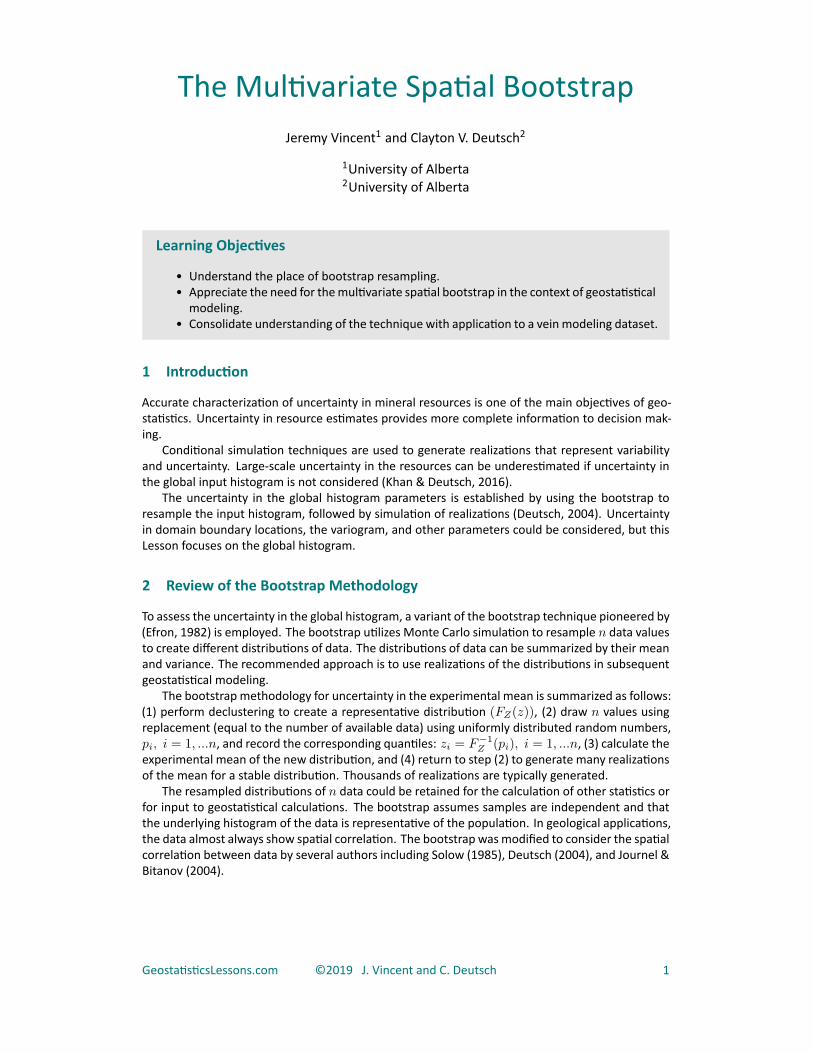
The Multivariate Spatial BootstrapJeremy Vincent1 and Clayton V. Deutsch2

1University of Alberta2University of Alberta

Learning Objectives

• Understand the place of bootstrap resampling.• Appreciate the need for themultivariate spatial bootstrap in the context of geostatistical

modeling.• Consolidate understanding of the technique with application to a vein modeling dataset.

1 Introduction

Accurate characterization of uncertainty in mineral resources is one of the main objectives of geo‐statistics. Uncertainty in resource estimates provides more complete information to decision mak‐ing.

Conditional simulation techniques are used to generate realizations that represent variabilityand uncertainty. Large‐scale uncertainty in the resources can be underestimated if uncertainty inthe global input histogram is not considered (Khan & Deutsch, 2016).

The uncertainty in the global histogram parameters is established by using the bootstrap toresample the input histogram, followed by simulation of realizations (Deutsch, 2004). Uncertaintyin domain boundary locations, the variogram, and other parameters could be considered, but thisLesson focuses on the global histogram.

2 Review of the Bootstrap Methodology

To assess the uncertainty in the global histogram, a variant of the bootstrap technique pioneered by(Efron, 1982) is employed. The bootstrap utilizes Monte Carlo simulation to resample n data valuesto create different distributions of data. The distributions of data can be summarized by their meanand variance. The recommended approach is to use realizations of the distributions in subsequentgeostatistical modeling.

The bootstrap methodology for uncertainty in the experimental mean is summarized as follows:(1) perform declustering to create a representative distribution (FZ(z)), (2) draw n values usingreplacement (equal to the number of available data) using uniformly distributed random numbers,pi, i = 1, ...n, and record the corresponding quantiles: zi = F−1

Z (pi), i = 1, ...n, (3) calculate theexperimental mean of the new distribution, and (4) return to step (2) to generate many realizationsof the mean for a stable distribution. Thousands of realizations are typically generated.

The resampled distributions of n data could be retained for the calculation of other statistics orfor input to geostatistical calculations. The bootstrap assumes samples are independent and thatthe underlying histogram of the data is representative of the population. In geological applications,the data almost always show spatial correlation. The bootstrap wasmodified to consider the spatialcorrelation between data by several authors including Solow (1985), Deutsch (2004), and Journel &Bitanov (2004).

GeostatisticsLessons.com ©2019 J. Vincent and C. Deutsch 1

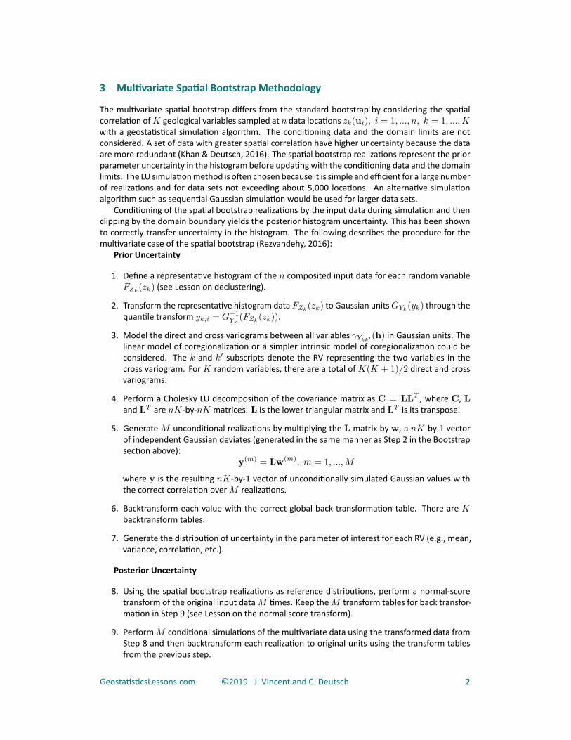
3 Multivariate Spatial Bootstrap Methodology

The multivariate spatial bootstrap differs from the standard bootstrap by considering the spatialcorrelation ofK geological variables sampled at n data locations zk(ui), i = 1, ..., n, k = 1, ...,Kwith a geostatistical simulation algorithm. The conditioning data and the domain limits are notconsidered. A set of data with greater spatial correlation have higher uncertainty because the dataare more redundant (Khan & Deutsch, 2016). The spatial bootstrap realizations represent the priorparameter uncertainty in the histogram before updating with the conditioning data and the domainlimits. The LU simulationmethod is often chosen because it is simple and efficient for a large numberof realizations and for data sets not exceeding about 5,000 locations. An alternative simulationalgorithm such as sequential Gaussian simulation would be used for larger data sets.

Conditioning of the spatial bootstrap realizations by the input data during simulation and thenclipping by the domain boundary yields the posterior histogram uncertainty. This has been shownto correctly transfer uncertainty in the histogram. The following describes the procedure for themultivariate case of the spatial bootstrap (Rezvandehy, 2016):

Prior Uncertainty

1. Define a representative histogram of the n composited input data for each random variableFZk

(zk) (see Lesson on declustering).

2. Transform the representative histogram dataFZk(zk) to Gaussian unitsGYk

(yk) through thequantile transform yk,i = G−1

Yk(FZk

(zk)).

3. Model the direct and cross variograms between all variables γYkk′ (h) in Gaussian units. Thelinear model of coregionalization or a simpler intrinsic model of coregionalization could beconsidered. The k and k′ subscripts denote the RV representing the two variables in thecross variogram. ForK random variables, there are a total ofK(K + 1)/2 direct and crossvariograms.

4. Perform a Cholesky LU decomposition of the covariance matrix as C = LLT , where C, Land LT are nK‐by‐nK matrices. L is the lower triangular matrix and LT is its transpose.

5. Generate M unconditional realizations by multiplying the L matrix by w, a nK‐by‐1 vectorof independent Gaussian deviates (generated in the same manner as Step 2 in the Bootstrapsection above):

y(m) = Lw(m), m = 1, ...,M

where y is the resulting nK‐by‐1 vector of unconditionally simulated Gaussian values withthe correct correlation overM realizations.

6. Backtransform each value with the correct global back transformation table. There are Kbacktransform tables.

7. Generate the distribution of uncertainty in the parameter of interest for each RV (e.g., mean,variance, correlation, etc.).

Posterior Uncertainty

8. Using the spatial bootstrap realizations as reference distributions, perform a normal‐scoretransform of the original input dataM times. Keep theM transform tables for back transfor‐mation in Step 9 (see Lesson on the normal score transform).

9. PerformM conditional simulations of the multivariate data using the transformed data fromStep 8 and then backtransform each realization to original units using the transform tablesfrom the previous step.

GeostatisticsLessons.com ©2019 J. Vincent and C. Deutsch 2

Figure 1: The multivariate spatial bootstrap workflow; Hist = histogram, Hist_ps = posterior, Real =realization.

10. Clip the realizations to the domain limits.

The spatial bootstrap process is sketched:

4 Example

Input DataThe following example utilizes a two‐dimensional, multivariate geological data set containingn = 67composited drill hole data. Compositing ensures the samples are equally weighted. The data arebounded by a 50m domain clipping limit (Figure 2). The variables of interest are thickness (Th) andgold (Au) (K = 2). They are spatially correlated (ρTh:Au = 0.50), with higher values generallylocated in the upper half of the domain. Declustering was undertaken using a 90m x 90m grid togenerate the representative distributions.

The data are normal‐score transformed for variogram modeling and spatial bootstrap resam‐pling. The direct experimental variograms are modeled using a single spherical structure, withranges of 250m and 165m for Th and Au respectively (Figure 3). An intrinsic model of coregional‐ization is used to scale the cross‐covariance between the two variables. A range of 250m is used forboth Th and Au in this step because Th is the primary variable of interest.

Prior Histogram UncertaintyUnconditional LU simulation is used to simulate M = 200 realizations of the declustered Th andAu distributions, each containing n = 67 data points. These are displayed as the green lines in thecumulative probability plots in the upper graphs of Figure 4. The variability of these realizationsreflects the resampling of the drill holes considering only the data locations and the covariance, notthe data values or the domain limits.

Each realization is averaged to create a distribution of 200 mean values that are plotted in thebottom of Figure 4. These histograms represent the prior uncertainty distributions of each variable.The mean values of Th and Au compare very closely to the mean values of the declustered distri‐butions. The uncertainty in the histograms is large due to the correlation of Th andAu. Recall that

GeostatisticsLessons.com ©2019 J. Vincent and C. Deutsch 3

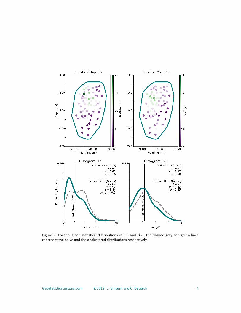
Figure 2: Locations and statistical distributions of Th and Au. The dashed gray and green linesrepresent the naive and the declustered distributions respectively.

GeostatisticsLessons.com ©2019 J. Vincent and C. Deutsch 4

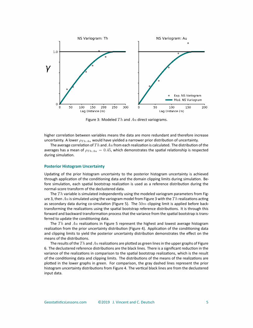
Figure 3: Modeled Th and Au direct variograms.

higher correlation between variables means the data are more redundant and therefore increaseuncertainty. A lower ρTh:Au would have yielded a narrower prior distribution of uncertainty.

The average correlation ofTh andAu from each realization is calculated. The distribution of theaverages has a mean of ρTh:Au = 0.45, which demonstrates the spatial relationship is respectedduring simulation.

Posterior Histogram UncertaintyUpdating of the prior histogram uncertainty to the posterior histogram uncertainty is achievedthrough application of the conditioning data and the domain clipping limits during simulation. Be‐fore simulation, each spatial bootstrap realization is used as a reference distribution during thenormal‐score transform of the declustered data.

The Th variable is simulated independently using the modeled variogram parameters from Fig‐ure 3, thenAu is simulated using the variogrammodel from Figure 3 with the Th realizations actingas secondary data during co‐simulation (Figure 5). The 50m clipping limit is applied before back‐transforming the realizations using the spatial bootstrap reference distributions. It is through thisforward and backward transformation process that the variance from the spatial bootstrap is trans‐ferred to update the conditioning data.

The Th and Au realizations in Figure 5 represent the highest and lowest average histogramrealization from the prior uncertainty distribution (Figure 4). Application of the conditioning dataand clipping limits to yield the posterior uncertainty distribution demonstrates the effect on themeans of the distributions.

The results of the Th andAu realizations are plotted as green lines in the upper graphs of Figure6. The declustered reference distributions are the black lines. There is a significant reduction in thevariance of the realizations in comparison to the spatial bootstrap realizations, which is the resultof the conditioning data and clipping limits. The distributions of the means of the realizations areplotted in the lower graphs in green. For comparison, the gray dashed lines represent the priorhistogram uncertainty distributions from Figure 4. The vertical black lines are from the declusteredinput data.

GeostatisticsLessons.com ©2019 J. Vincent and C. Deutsch 5

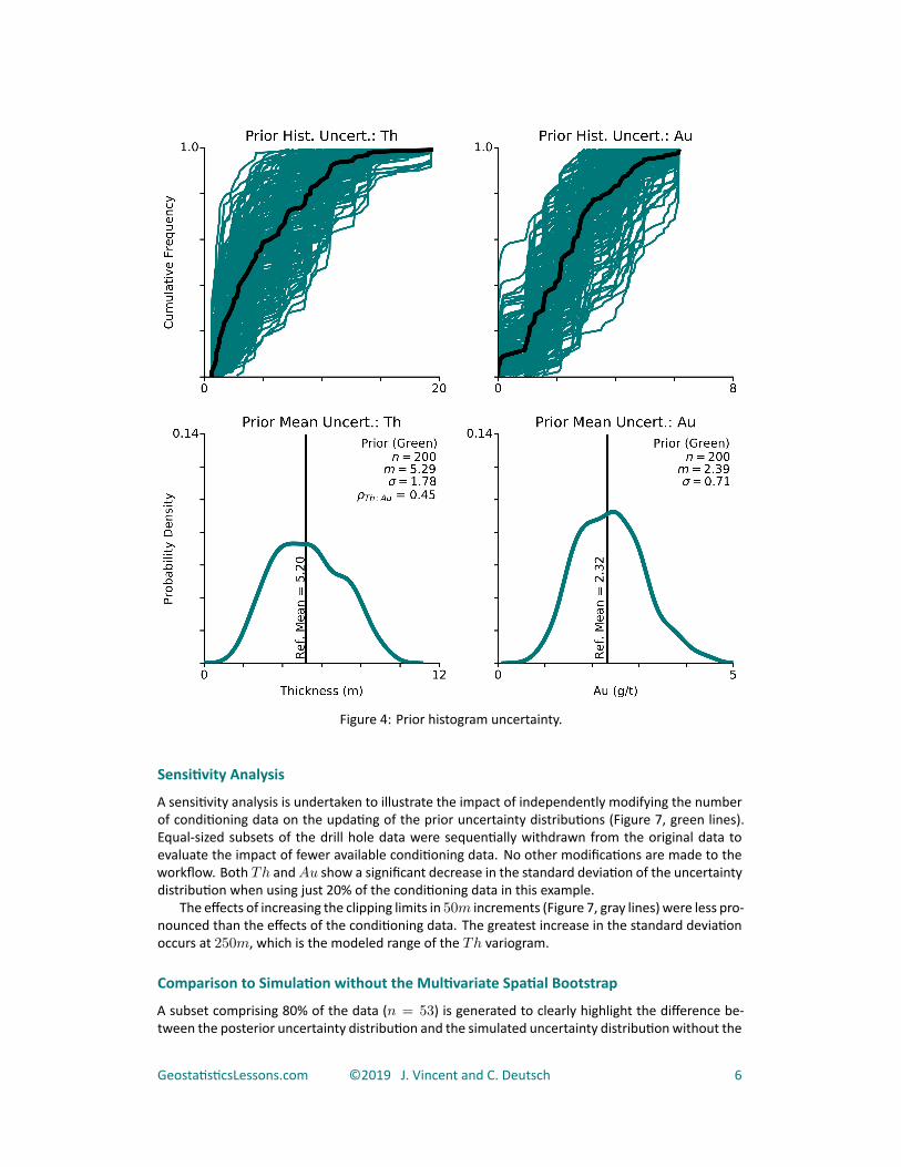
Figure 4: Prior histogram uncertainty.

Sensitivity AnalysisA sensitivity analysis is undertaken to illustrate the impact of independently modifying the numberof conditioning data on the updating of the prior uncertainty distributions (Figure 7, green lines).Equal‐sized subsets of the drill hole data were sequentially withdrawn from the original data toevaluate the impact of fewer available conditioning data. No other modifications are made to theworkflow. Both Th andAu show a significant decrease in the standard deviation of the uncertaintydistribution when using just 20% of the conditioning data in this example.

The effects of increasing the clipping limits in 50m increments (Figure 7, gray lines) were less pro‐nounced than the effects of the conditioning data. The greatest increase in the standard deviationoccurs at 250m, which is the modeled range of the Th variogram.

Comparison to Simulation without the Multivariate Spatial BootstrapA subset comprising 80% of the data (n = 53) is generated to clearly highlight the difference be‐tween the posterior uncertainty distribution and the simulated uncertainty distributionwithout the

GeostatisticsLessons.com ©2019 J. Vincent and C. Deutsch 6

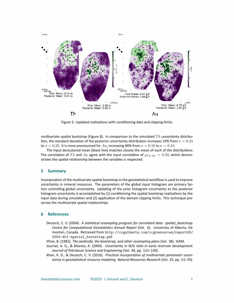
Figure 5: Updated realizations with conditioning data and clipping limits.

multivariate spatial bootstrap (Figure 8). In comparison to the simulated Th uncertainty distribu‐tion, the standard deviation of the posterior uncertainty distribution increases 33% from σ = 0.24to σ = 0.32. It is more pronounced for Au, increasing 80% from σ = 0.10 to σ = 0.18.

The input declustered mean (black line) matches closely the mean of each of the distributions.The correlation of Th and Au agree with the input correlation of ρTh:Au = 0.50, which demon‐strates the spatial relationship between the variables is respected.

5 Summary

Incorporation of the multivariate spatial bootstrap in the geostatistical workflow is used to improveuncertainty in mineral resources. The parameters of the global input histogram are primary fac‐tors controlling global uncertainty. Updating of the prior histogram uncertainty to the posteriorhistogram uncertainty is accomplished by (1) conditioning the spatial bootstrap realizations by theinput data during simulation and (2) application of the domain clipping limits. This technique pre‐serves the multivariate spatial relationships.

6 References

Deutsch, C. V. (2004). A statistical resampling program for correlated data: spatial_bootstrap.Centre for Computational Geostatistics Annual Report (Vol. 6). University of Alberta, Ed‐monton, Canada. Retrieved from http://ccgalberta.com/ccgresources/report06/2004-401-spatial_bootstrap.pdf

Efron, B. (1982). The jackknife, the bootstrap, and other resampling plans (Vol. 38). SIAM.Journel, A. G., & Bitanov, A. (2004). Uncertainty in N/G ratio in early reservoir development.

Journal of Petroleum Science and Engineering (Vol. 44, pp. 115–130).Khan, K. D., & Deutsch, C. V. (2016). Practical incorporation of multivariate parameter uncer‐

tainty in geostatistical resource modeling. Natural Resources Research (Vol. 25, pp. 51–70).

GeostatisticsLessons.com ©2019 J. Vincent and C. Deutsch 7

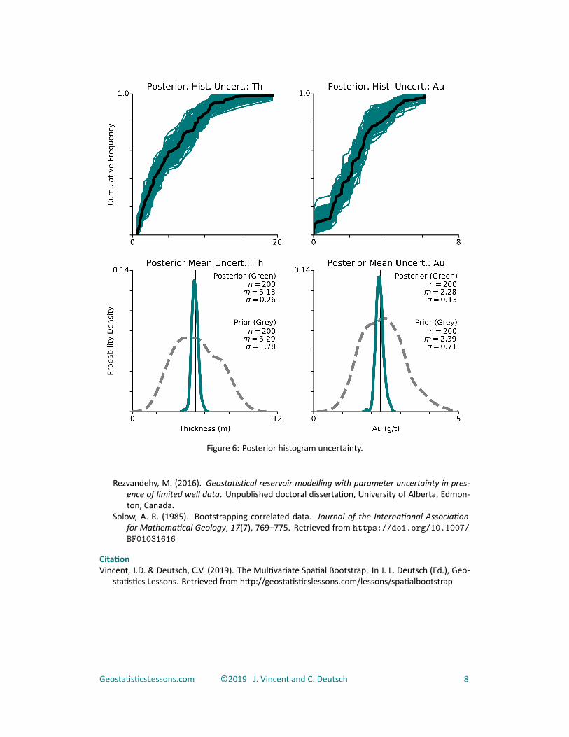
Figure 6: Posterior histogram uncertainty.

Rezvandehy, M. (2016). Geostatistical reservoir modelling with parameter uncertainty in pres‐ence of limited well data. Unpublished doctoral dissertation, University of Alberta, Edmon‐ton, Canada.

Solow, A. R. (1985). Bootstrapping correlated data. Journal of the International Associationfor Mathematical Geology, 17(7), 769–775. Retrieved from https://doi.org/10.1007/BF01031616

CitationVincent, J.D. & Deutsch, C.V. (2019). The Multivariate Spatial Bootstrap. In J. L. Deutsch (Ed.), Geo‐

statistics Lessons. Retrieved from http://geostatisticslessons.com/lessons/spatialbootstrap

GeostatisticsLessons.com ©2019 J. Vincent and C. Deutsch 8

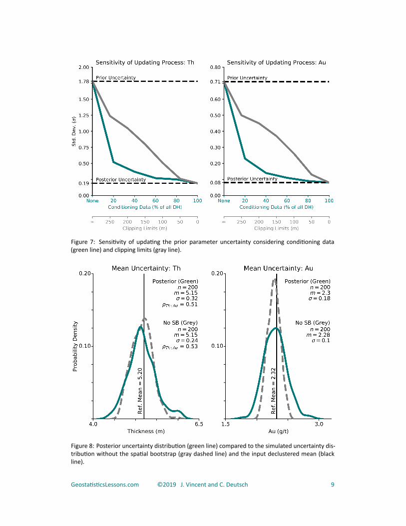
Figure 7: Sensitivity of updating the prior parameter uncertainty considering conditioning data(green line) and clipping limits (gray line).

Figure 8: Posterior uncertainty distribution (green line) compared to the simulated uncertainty dis‐tribution without the spatial bootstrap (gray dashed line) and the input declustered mean (blackline).

GeostatisticsLessons.com ©2019 J. Vincent and C. Deutsch 9