Embed Size (px)
Citation preview

The XSB System
Version 3.3
Volume 2: Libraries, Interfaces and Packages
xsb
July 4, 2013

Credits
Interfaces have become an increasingly important part of XSB. The interface from C toProlog was implemented by David Warren as was the DLL interface; the interface fromProlog to C (foreign language interface) was developed by Jiyang Xu, Kostis Sagonasand Steve Dawson. The Oracle interface was written by Hassan Davulcu and ErnieJohnson. The ODBC took as its starting point the Oracle interface, and was writtenby Lily Dong and Baoqiu Cui, and maintained by David Warren. The interface toPOSIX regular expression and wildcard matching as well as the Libwww-based Webaccess package was written by Michael Kifer. The interface to Perl pattern matchingroutines was written by Michael Kifer and Jin Yu. The SModels interface was writtenby Luis F. Castro.
The SLX preprocessor was written by José Júlio Alferes and Luís Moniz Pereira. Unix-style scripting libraries were written by Terrance Swift, and the ordset library waswritten by Richard O’Keefe.

Contents
1 Library Utilities 1
1.1 List Processing . . . . . . . . . . . . . . . . . . . . . . . . . . . . . . . . . . . . . . . 1
1.1.1 Processing Comma Lists . . . . . . . . . . . . . . . . . . . . . . . . . . . . . . 3
1.2 Attributed Variables . . . . . . . . . . . . . . . . . . . . . . . . . . . . . . . . . . . . 3
1.2.1 Lowlevel Interface . . . . . . . . . . . . . . . . . . . . . . . . . . . . . . . . . 4
1.3 constraintLib: a library for CLP . . . . . . . . . . . . . . . . . . . . . . . . . . . . 7
1.4 Formatted Output . . . . . . . . . . . . . . . . . . . . . . . . . . . . . . . . . . . . . 9
1.5 String Manipulation . . . . . . . . . . . . . . . . . . . . . . . . . . . . . . . . . . . . 11
1.6 Script Writing Utilities . . . . . . . . . . . . . . . . . . . . . . . . . . . . . . . . . . . 12
1.6.1 Communication with Subprocesses . . . . . . . . . . . . . . . . . . . . . . . . 14
1.7 Socket I/O . . . . . . . . . . . . . . . . . . . . . . . . . . . . . . . . . . . . . . . . . 21
1.8 Arrays . . . . . . . . . . . . . . . . . . . . . . . . . . . . . . . . . . . . . . . . . . . . 26
1.9 The Profiling Library . . . . . . . . . . . . . . . . . . . . . . . . . . . . . . . . . . . . 27
1.10 Gensym . . . . . . . . . . . . . . . . . . . . . . . . . . . . . . . . . . . . . . . . . . . 29
1.11 Random Number Generator . . . . . . . . . . . . . . . . . . . . . . . . . . . . . . . . 29
1.12 Loading Separated Files . . . . . . . . . . . . . . . . . . . . . . . . . . . . . . . . . . 31
1.13 Scanning in Prolog . . . . . . . . . . . . . . . . . . . . . . . . . . . . . . . . . . . . . 32
1.14 XSB Lint . . . . . . . . . . . . . . . . . . . . . . . . . . . . . . . . . . . . . . . . . . 33
1.15 Miscellaneous Predicates . . . . . . . . . . . . . . . . . . . . . . . . . . . . . . . . . . 34
1.16 Other Libraries . . . . . . . . . . . . . . . . . . . . . . . . . . . . . . . . . . . . . . . 35
1.16.1 Justification . . . . . . . . . . . . . . . . . . . . . . . . . . . . . . . . . . . . . 35
1.16.2 AVL Trees . . . . . . . . . . . . . . . . . . . . . . . . . . . . . . . . . . . . . . 35
1.16.3 Ordered Sets: ordsets.P . . . . . . . . . . . . . . . . . . . . . . . . . . . . . 36
1.16.4 Unweighted Graphs: ugraphs.P . . . . . . . . . . . . . . . . . . . . . . . . . 36
i
CONTENTS ii
1.16.5 Heaps: heaps.P . . . . . . . . . . . . . . . . . . . . . . . . . . . . . . . . . . 36
2 XSB-ODBC Interface 38
2.1 Introduction . . . . . . . . . . . . . . . . . . . . . . . . . . . . . . . . . . . . . . . . . 38
2.2 Using the Interface . . . . . . . . . . . . . . . . . . . . . . . . . . . . . . . . . . . . . 39
2.2.1 Connecting to and Disconnecting from Data Sources . . . . . . . . . . . . . . 39
2.2.2 Accessing Tables in Data Sources Using SQL . . . . . . . . . . . . . . . . . . 40
2.2.3 Cursor Management . . . . . . . . . . . . . . . . . . . . . . . . . . . . . . . . 42
2.2.4 Accessing Tables in Data Sources through the Relation Level . . . . . . . . . 42
2.2.5 Using the Relation Level Interface . . . . . . . . . . . . . . . . . . . . . . . . 43
2.2.6 Handling NULL values . . . . . . . . . . . . . . . . . . . . . . . . . . . . . . . 44
2.2.7 The View Level Interface . . . . . . . . . . . . . . . . . . . . . . . . . . . . . 46
2.2.8 Insertions and Deletions of Rows through the Relational Level . . . . . . . . 48
2.2.9 Access to Data Dictionaries . . . . . . . . . . . . . . . . . . . . . . . . . . . . 50
2.2.10 Other Database Operations . . . . . . . . . . . . . . . . . . . . . . . . . . . . 50
2.2.11 Transaction Management . . . . . . . . . . . . . . . . . . . . . . . . . . . . . 51
2.2.12 Interface Flags . . . . . . . . . . . . . . . . . . . . . . . . . . . . . . . . . . . 51
2.2.13 Datalog . . . . . . . . . . . . . . . . . . . . . . . . . . . . . . . . . . . . . . . 52
2.3 Error messages . . . . . . . . . . . . . . . . . . . . . . . . . . . . . . . . . . . . . . . 53
2.4 Notes on specific ODBC drivers . . . . . . . . . . . . . . . . . . . . . . . . . . . . . . 53
3 The New XSB-Database Interface 54
3.1 Introduction . . . . . . . . . . . . . . . . . . . . . . . . . . . . . . . . . . . . . . . . . 54
3.2 Configuring the Interface . . . . . . . . . . . . . . . . . . . . . . . . . . . . . . . . . 54
3.3 Using the Interface . . . . . . . . . . . . . . . . . . . . . . . . . . . . . . . . . . . . . 57
3.3.1 Connecting to and Disconnecting from Databases . . . . . . . . . . . . . . . . 57
3.3.2 Querying Databases . . . . . . . . . . . . . . . . . . . . . . . . . . . . . . . . 58
3.4 Error Handling . . . . . . . . . . . . . . . . . . . . . . . . . . . . . . . . . . . . . . . 59
3.5 Notes on specific drivers . . . . . . . . . . . . . . . . . . . . . . . . . . . . . . . . . . 61
4 Introduction to XSB Packages 63
5 Wildcard Matching 64

CONTENTS iii
6 pcre: Pattern Matching and Substitution Using PCRE 66
6.1 Introduction . . . . . . . . . . . . . . . . . . . . . . . . . . . . . . . . . . . . . . . . . 66
6.2 Pattern matching . . . . . . . . . . . . . . . . . . . . . . . . . . . . . . . . . . . . . . 66
6.3 String Substitution . . . . . . . . . . . . . . . . . . . . . . . . . . . . . . . . . . . . . 67
6.4 Installation and configuration . . . . . . . . . . . . . . . . . . . . . . . . . . . . . . . 68
6.4.1 Configuring for Linux, Mac, and other Unices . . . . . . . . . . . . . . . . . . 68
6.4.2 Configuring for Windows . . . . . . . . . . . . . . . . . . . . . . . . . . . . . 68
7 curl: The XSB Internet Access Package 70
7.1 Introduction . . . . . . . . . . . . . . . . . . . . . . . . . . . . . . . . . . . . . . . . . 70
7.2 Integration with File I/O . . . . . . . . . . . . . . . . . . . . . . . . . . . . . . . . . 70
7.2.1 Opening a Web Document . . . . . . . . . . . . . . . . . . . . . . . . . . . . . 71
7.2.2 Closing a Web Document . . . . . . . . . . . . . . . . . . . . . . . . . . . . . 71
7.3 Low Level Predicates . . . . . . . . . . . . . . . . . . . . . . . . . . . . . . . . . . . . 72
7.3.1 Loading web documents . . . . . . . . . . . . . . . . . . . . . . . . . . . . . . 72
7.3.2 Retrieve the properties of a web document . . . . . . . . . . . . . . . . . . . 72
7.3.3 Encode Url . . . . . . . . . . . . . . . . . . . . . . . . . . . . . . . . . . . . . 72
7.3.4 Obtaining the Redirection URL . . . . . . . . . . . . . . . . . . . . . . . . . . 73
7.4 Installation and configuration . . . . . . . . . . . . . . . . . . . . . . . . . . . . . . . 73
8 sgml and xpath: SGML/XML/HTML Parsers and XPath 74
8.1 Introduction . . . . . . . . . . . . . . . . . . . . . . . . . . . . . . . . . . . . . . . . . 74
8.2 Overview of the SGML Parser . . . . . . . . . . . . . . . . . . . . . . . . . . . . . . . 75
8.3 Predicate Reference . . . . . . . . . . . . . . . . . . . . . . . . . . . . . . . . . . . . 76
8.3.1 Loading Structured Documents . . . . . . . . . . . . . . . . . . . . . . . . . . 76
8.3.2 Handling of White Spaces . . . . . . . . . . . . . . . . . . . . . . . . . . . . . 79
8.3.3 XML documents . . . . . . . . . . . . . . . . . . . . . . . . . . . . . . . . . . 79
8.3.4 DTD-Handling . . . . . . . . . . . . . . . . . . . . . . . . . . . . . . . . . . . 80
8.3.5 Low-level Parsing Primitives . . . . . . . . . . . . . . . . . . . . . . . . . . . 81
8.3.6 External Entities . . . . . . . . . . . . . . . . . . . . . . . . . . . . . . . . . . 84
8.3.7 Exceptions . . . . . . . . . . . . . . . . . . . . . . . . . . . . . . . . . . . . . 84
8.3.8 Unsupported features . . . . . . . . . . . . . . . . . . . . . . . . . . . . . . . 85
8.3.9 Summary of Predicates . . . . . . . . . . . . . . . . . . . . . . . . . . . . . . 86

CONTENTS iv
8.4 XPath support . . . . . . . . . . . . . . . . . . . . . . . . . . . . . . . . . . . . . . . 86
9 rdf: The XSB RDF Parser 89
9.1 Introduction . . . . . . . . . . . . . . . . . . . . . . . . . . . . . . . . . . . . . . . . . 89
9.2 High-level API . . . . . . . . . . . . . . . . . . . . . . . . . . . . . . . . . . . . . . . 89
9.2.1 RDF Object representation . . . . . . . . . . . . . . . . . . . . . . . . . . . . 90
9.2.2 Name spaces . . . . . . . . . . . . . . . . . . . . . . . . . . . . . . . . . . . . 91
9.2.3 Low-level access . . . . . . . . . . . . . . . . . . . . . . . . . . . . . . . . . . 91
9.3 Testing the RDF translator . . . . . . . . . . . . . . . . . . . . . . . . . . . . . . . . 92
10 Constraint Packages 93
10.1 clpr: The CPL(R) package . . . . . . . . . . . . . . . . . . . . . . . . . . . . . . . . 93
10.1.1 The CLP(R) API . . . . . . . . . . . . . . . . . . . . . . . . . . . . . . . . . . 94
10.2 The bounds Package . . . . . . . . . . . . . . . . . . . . . . . . . . . . . . . . . . . . 99
10.2.1 The bounds API . . . . . . . . . . . . . . . . . . . . . . . . . . . . . . . . . . 101
11 Constraint Handling Rules 104
11.1 Introduction . . . . . . . . . . . . . . . . . . . . . . . . . . . . . . . . . . . . . . . . . 104
11.2 Syntax and Semantics . . . . . . . . . . . . . . . . . . . . . . . . . . . . . . . . . . . 104
11.2.1 Syntax . . . . . . . . . . . . . . . . . . . . . . . . . . . . . . . . . . . . . . . . 104
11.2.2 Semantics . . . . . . . . . . . . . . . . . . . . . . . . . . . . . . . . . . . . . . 105
11.3 CHR in XSB Programs . . . . . . . . . . . . . . . . . . . . . . . . . . . . . . . . . . 107
11.3.1 Embedding in XSB Programs . . . . . . . . . . . . . . . . . . . . . . . . . . . 107
11.3.2 Compilation . . . . . . . . . . . . . . . . . . . . . . . . . . . . . . . . . . . . . 107
11.4 Useful Predicates . . . . . . . . . . . . . . . . . . . . . . . . . . . . . . . . . . . . . . 108
11.5 Examples . . . . . . . . . . . . . . . . . . . . . . . . . . . . . . . . . . . . . . . . . . 108
11.6 CHR and Tabling . . . . . . . . . . . . . . . . . . . . . . . . . . . . . . . . . . . . . . 109
11.6.1 General Issues and Principles . . . . . . . . . . . . . . . . . . . . . . . . . . . 109
11.6.2 Call Abstraction . . . . . . . . . . . . . . . . . . . . . . . . . . . . . . . . . . 110
11.6.3 Answer Projection . . . . . . . . . . . . . . . . . . . . . . . . . . . . . . . . . 110
11.6.4 Answer Combination . . . . . . . . . . . . . . . . . . . . . . . . . . . . . . . . 112
11.6.5 Overview of Tabling-related Predicates . . . . . . . . . . . . . . . . . . . . . . 114
11.7 Guidelines . . . . . . . . . . . . . . . . . . . . . . . . . . . . . . . . . . . . . . . . . . 114

CONTENTS v
11.8 CHRd . . . . . . . . . . . . . . . . . . . . . . . . . . . . . . . . . . . . . . . . . . . . 114
12 XASP: Answer Set Programming with XSB and Smodels 116
12.1 Installing the Interface . . . . . . . . . . . . . . . . . . . . . . . . . . . . . . . . . . . 117
12.1.1 Installing the Interface under Unix . . . . . . . . . . . . . . . . . . . . . . . . 117
12.1.2 Installing XASP under Windows using Cygwin . . . . . . . . . . . . . . . . . 118
12.2 The Smodels Interface . . . . . . . . . . . . . . . . . . . . . . . . . . . . . . . . . . . 120
12.2.1 Using the Smodels Interface with Multiple Threads . . . . . . . . . . . . . . . 123
12.3 The xnmr_int Interface . . . . . . . . . . . . . . . . . . . . . . . . . . . . . . . . . . 123
13 PITA: Probabilistic Inference with Tabling and Answer subsumption 126
13.0.1 Installation . . . . . . . . . . . . . . . . . . . . . . . . . . . . . . . . . . . . . 126
13.0.2 Use . . . . . . . . . . . . . . . . . . . . . . . . . . . . . . . . . . . . . . . . . 128
14 Other XSB Packages 130
14.1 Programming with FLORA-2 . . . . . . . . . . . . . . . . . . . . . . . . . . . . . . . 130
14.2 Summary of xmc: Model-checking with XSB . . . . . . . . . . . . . . . . . . . . . . 132
14.3 slx: Extended Logic Programs under the Well-Founded Semantics . . . . . . . . . . 133
14.4 gapza: Generalized Annotated Programs . . . . . . . . . . . . . . . . . . . . . . . . . 135
Chapter 1
Library Utilities
In this chapter we introduce libraries of some useful predicates that are supplied with XSB. Inter-faces and more elaborate packages are documented in later chapters. These predicates are availableonly when imported them from (or explicitly consult) the corresponding modules.
1.1 List Processing
The XSB library contains various list utilities, some of which are listed below. These predicatesshould be explicitly imported from the module specified after the skeletal specification of eachpredicate. There are a lot more useful list processing predicates in various modules of the XSBsystem, and the interested user can find them by looking at the sources.
append(?List1, ?List2, ?List3) module: basics
Succeeds if list List3 is the concatenation of lists List1 and List2.
member(?Element, ?List) module: basics
Checks whether Element unifies with any element of list List, succeeding more than once ifthere are multiple such elements.
memberchk(?Element, ?List) module: basics
Similar to member/2, except that memberchk/2 is deterministic, i.e. does not succeed morethan once for any call.
ith(?Index, ?List, ?Element) module: basics
Succeeds if the Indexth element of the list List unifies with Element. Fails if Index is nota positive integer or greater than the length of List. Either Index and List, or List andElement, should be instantiated (but not necessarily ground) at the time of the call.
delete_ith(+Index, +List, ?Element, ?RestList) module: listutil
Succeeds if the Indexth element of the list List unifies with Element, and RestList is List
with Element removed. Fails if Index is not a positive integer or greater than the length ofList.
1
CHAPTER 1. LIBRARY UTILITIES 2
log_ith(?Index, ?Tree, ?Element) module: basics
Succeeds if the Indexth element of the Tree Tree unifies with Element. Fails if Index is nota positive integer or greater than the number of elements that can be in Tree. Either Index
and Tree, or Tree and Element, should be instantiated (but not necessarily ground) at thetime of the call. Tree is a list of full binary trees, the first being of depth 0, and each onebeing of depth one greater than its predecessor. So log_ith/3 is very similar to ith/3 exceptit uses a tree instead of a list to obtain log-time access to its elements.
log_ith_bound(?Index, ?Tree, ?Element) module: basics
is like log_ith/3, but only if the Indexth element of Tree is non-variable and equal toElement. This predicate can be used in both directions, and is most useful with Indexunbound, since it will then bind Index and Element for each non-variable element in Tree
(in time proportional to N ∗ logN , for N the number of non-variable entries in Tree.)
length(?List, ?Length) module: basics
Succeeds if the length of the list List is Length. This predicate is deterministic if List isinstantiated to a list of definite length, but is nondeterministic if List is a variable or has avariable tail. If List is uninstantiated, it is unified with a list of length Length that containsvariables.
same_length(?List1, ?List2) module: basics
Succeeds if list List1 and List2 are both lists of the same number of elements. No relationbetween the types or values of their elements is implied. This predicate may be used togenerate either list (containing variables as elements) given the other, or to generate two listsof the same length, in which case the arguments will be bound to lists of length 0, 1, 2, . . ..
select(?Element, ?L1, ?L2) module: basics
List2 derives from List1 by selecting (removing) an Element non-deterministically.
reverse(+List, ?ReversedList) module: basics
Succeeds if ReversedList is the reverse of list List. If List is not a proper list, reverse/2
can succeed arbitrarily many times. It works only one way.
perm(+List, ?Perm) module: basics
Succeeds when List and Perm are permutations of each other. The main use of perm/2 isto generate permutations of a given list. List must be a proper list. Perm may be partlyinstantiated.
subseq(?Sequence, ?SubSequence, ?Complement) module: basics
Succeeds when SubSequence and Complement are both subsequences of the list Sequence
(the order of corresponding elements being preserved) and every element of Sequence whichis not in SubSequence is in the Complement and vice versa. That is,
length(Sequence) = length(SubSequence) + length(Complement)
for example, subseq([1,2,3,4], [1,3], [2,4]). The main use of subseq/3 is to generatesubsets and their complements together, but can also be used to interleave two lists in allpossible ways.
CHAPTER 1. LIBRARY UTILITIES 3
merge(+List1, +List2, ?List3) module: listutil
Succeeds if List3 is the list resulting from “merging” lists List1 and List2, i.e. the elementsof List1 together with any element of List2 not occurring in List1. If List1 or List2 containduplicates, List3 may also contain duplicates.
absmerge(+List1, +List2, ?List3) module: listutil
Predicate absmerge/3 is similar to merge/3, except that it uses predicate absmember/2
described below rather than member/2.
absmember(+Element, +List) module: listutil
Similar to member/2, except that it checks for identity (through the use of predicate ’==’/2)rather than unifiability (through ’=’/2) of Element with elements of List.
member2(?Element, ?List) module: listutil
Checks whether Element unifies with any of the actual elements of List. The only differ-ence between this predicate and predicate member/2 is on lists having a variable tail, e.g.[a, b, c | _ ]: while member/2 would insert Element at the end of such a list if it did notfind it, Predicate member2/2 only checks for membership but does not insert the Element
into the list if it is not there.
closetail(?List) module: listutil
Predicate closetail/1 closes the tail of an open-ended list. It succeeds only once.
1.1.1 Processing Comma Lists
It is often useful to process comma lists when meta-interpreting or preprocessing. XSB librariesinclude the following simple utilities.
comma_to_list(+CommaList,-List) module: basics
Transforms CommaList to List.
comma_append(?CL1,?CL2,?CL3) basics
comma_length(?CommaList,?Length) basics
comma_member(?Element,?CommaList) basics
comma_member(?Element,?CommaList) module: basics
Analogues for comma lists of append/3, length/3, member/2 and memberchk/2, respectively.
1.2 Attributed Variables
Attributed variables are a special data type that associates variables with arbitrary attributesas well as supports extensible unification. Attributed variables have proven to be a flexible andpowerful mechanism to extend a classic logic programming system with the ability of constraintsolving. Our low-level API for constraints closely resembles that of hProlog [8] and SWI [31].

CHAPTER 1. LIBRARY UTILITIES 4
1.2.1 Lowlevel Interface
Attributes of variables are pairs of attribute module names and values. An attribute module namecan be any atom. A value can be any XSB value (term, variable, atom, . . . ). Any variable hasat most one attribute for a particular attribute module. Attribute modules are distinct from XSBmodules: although it is most efficient to keep each handlers for each attribute module in their ownXSB module. c Attributes can be manipulated with the following three predicates (get_attr/3,put_attr/3 and del_attr/2) defined in the module machine.
get_attr(-Var,+Mod, ?Val) module: machine
Gets the value of the attribute of Var in attribute module Mod. Non-variable terms in Var
cause a type error. Val will be unified with the value of the attribute, if it exists. Otherwisethe predicate fails.
put_attr(-Var,+Mod, ?Val) module: machine
Sets the value of the attribute of Var in attribute module Mod. Non-variable terms in Var
cause a type error. The previous value of the attribute is overwritten, if it exists.
del_attr(-Var, +Mod) module: machine
Removes the attribute of Var in attribute module Mod. Non-variable terms in Var cause atype error. The previous value of the attribute is removed, if it exists.
One has to extend the default unification algorithm for used attributes by installing a handlerin the following way:
:- install_verify_attribute_handler(+Mod,−AttrV alue,−Target, +Handler, +WarningF lag)
:- install_verify_attribute_handler(+Mod,−AttrV alue,−Target, +Handler)
The predicates install_verify_attribute_handler/5 and install_verify_attribute_handler/4
are defined in module machine. Mod is the attribute Module and Handler is a term with argumentsAttrV alue and Target. The Handler term has to correspond to a handler predicate that takes thevalue of the attribute (AttrV alue) and the term that the attributed value is bound to (Target) asarguments. The argument WarningF lag in the 5-argument version of the predicate can be usedto suppress the warning issued when replacing the verify_attribute_handler for a module. Ifthe argument is warning_on then the warning is issued if a handler for the module already exists.Otherwise, the warning is suppressed. The 4-argument version of the predicate does not suppressthe warning.
To get good efficiency, it is usually best to keep the handlers for each attribute module inseparate XSB modules. The handler is called after the unification of an attributed variable with aterm or other attributed variable, if the attributed variable has an attribute in the correspondingmodule. The two arguments of the unification are already bound at the time the handler is called,i.e. the handler is a post-unify handler.
Here, by giving the implementation of a simple finite domain constraint solver (see the file fd.P
below), we show how these lowlevel predicates for attributed variables can be used. In this example,an attribute in the module fd is used and the value of this attribute is a list of terms.

CHAPTER 1. LIBRARY UTILITIES 5
%% File: fd.P
%%
%% A simple finite domain constrait solver implemented using the lowlevel
%% attributes variables interface.
:- import put_attr/3, get_attr/3, del_attr/2,
install_verify_attribute_handler/4 from machine.
:- import member/2 from basics.
:- install_verify_attribute_handler(fd,AttrValue,Target,fd_handler(AttrValue,Target)).
fd_handler(Da, Target) :-
(var(Target), % Target is an attributed variable
get_attr(Target, fd, Db) -> % has a domain
intersection(Da, Db, [E|Es]), % intersection not empty
(Es = [] -> % exactly one element
Target = E % bind Var (and Value) to E
; put_attr(Target, fd, [E|Es]) % update Var’s (and Value’s)
)
; member(Target, Da) % is Target a member of Da?
).
intersection([], _, []).
intersection([H|T], L2, [H|L3]) :-
member(H, L2), !,
intersection(T, L2, L3).
intersection([_|T], L2, L3) :-
intersection(T, L2, L3).
domain(X, Dom) :-
var(Dom), !,
get_attr(X, fd, Dom).
domain(X, List) :-
List = [El|Els], % at least one element
(Els = [] % exactly one element
-> X = El % implied binding
; put_attr(Fresh, fd, List), % create a new attributed variable
X = Fresh % may call verify_attributes/2
).
show_domain(X) :- % print out the domain of X
var(X), % X must be a variable
get_attr(X, fd, D),
write(’Domain of ’), write(X),
write(’ is ’), writeln(D).
When writing or porting a constraint package, it is usually useful to adjust the way that correctanswer substitutions are shown in the command line. This can be controlled using the followingtwo predicates:

CHAPTER 1. LIBRARY UTILITIES 6
install_attribute_portray_hook(Module,Attribute,Handler) module: machineThis hook is called by the command-line interpreter when printing out the value of each
variable in a top-level query. When a printing out an attributed variable, any appropriatehandlers are called to portray the constraints represented by the attribute. As an example,the bounds package (Section 10.2) uses a hook to print out the bounds of variables:
| ?- X in 1..10,Y in 1..10,X + 4 #< Y -3.
X = _h629 { bounds : 1 .. 2 }
Y = _h673 { bounds : 9 .. 10 }
Writing a handler can be as simple as possible or as elaborate as desired. In the case ofbounds the handler is simple:
bounds_attr_portray_hook(bounds(L,U,_)) :- write(L..U).
The hook is installed when the constraint package is loaded by placing in the package loaderdirective such as:
:- install_attribute_portray_hook(bounds,Attr,bounds_attr_portray_hook(Attr)).
Note that the hook will be indexed on the module associated with the attribute (in this casebounds). XSB’s command-line interpreter will unify the second argument of the portray hookwith the attribute, and then call Handler.
install_attribute_constraint_hook(Module,Vars,Names,Handler) module: machineFor some constraint packages, it may not be particularly useful to associate constraints with
variables: instead, the projection of global constraints onto the variables of the top-levelquery may be more useful. This is the case in the CLP(R) package (Section 10.1), where thecommand-line interaction may look as follows:
| ?- {X = 2*Y,Y >= 7},inf(X,F).
{ X >= 14.0000 }
{ Y = 0.5000 * X }
X = _h8841
Y = _h9506
F = 14.0000
In XSB, the (projection of the) global constraints in CLP(R) are displayed by the followingroutines:
clpr_portray_varlist(Vars,Names):-
filter_varlist(Vars,Names,V1,N1),
dump(V1,N1,Constraints),
member(C,Constraints),
console_write(’ { ’), console_write(C),console_writeln(’ } ’),
fail.
clpr_portray_varlist(_V,_N).
filter_varlist([],[],[],[]).
filter_varlist([V1|R1],[N1|R2],[V1|R3],[N1|R4]):-

CHAPTER 1. LIBRARY UTILITIES 7
var(V1),!,
filter_varlist(R1,R2,R3,R4).
filter_varlist([_V1|R1],[_N1|R2],R3,R4):-
filter_varlist(R1,R2,R3,R4).
This predicate sets up a call to the CLP(R) library predicate dump/3, whose constraints itthen writes out to the console. Analogous to the portray hook, the console hook is installedusing the directive:
:- install_constraint_portray_hook(clpr,Vars,Names,clpr_portray_varlist(Vars,Names)).
If the clpr module is loaded, the command line interpreter checks any constraint portrayhooks upon the first success of a top-level goal. It then unifies the second argument Vars
with the variables of the goal, and Names with the names of the variables of the goal whichare then passed on to Handler
1.3 constraintLib: a library for CLP
XSB supports constraint logic programming through its engine-level support of attributed vari-ables (Section 1.2), and its support for constraint handling rules (CHR) (Chapter 11). TheconstraintLib library includes routines for delaying and examining bindings that are commonlyused to implement CHR and other constraint libraries.
When processing constraints, it is often useful to delay a goal based on the instantiation levelof a term or set of terms. For instance a 3 > X + Y should be delayed until both X and Y areinstantiated. However the goal should be reinvoked as soon as possible after both are instantiatedin order to prune search paths that may not be useful to pursue. The predicate when/2 provides auseful mechanism to delay goals based on instantiation patterns 1.
when(+Condition,Goal) module: constraintLib
Delays the execution of Goal until Condition is satisfied, whereupon Goal will be executed.Condition can have the form
• ?=(Term1,Term2)
• nonvar(Term)
• ground(Term) 2
• (Condition,Condition)
• (Condition ; Condition)
Example: The following session illustrates the use of when/2 to delay a goal.
1Despite the similar name, this method of delaying is conceptually different from SLG delaying discussed inVolume 1 of this manual, which is used for resolving cycles of dependencies in computing the well-founded semantics,and is not based on the state of instantiation of a term.
2To use ground/1 in the condition, it must be imported into the file where it is used.
CHAPTER 1. LIBRARY UTILITIES 8
|?- when(nonvar(X),writeln(test(1-2,nonvar))),writeln(test(1,nonvar)),X = f(_Y).
test(1,nonvar)
test(1 - 2,nonvar)
X = f(_h245)
unifiable(X, Y, -Unifier) module: constraintLib
If X and Y can unify, succeeds unifying Unifier with a list of terms of the form Var =
Value representing a most general unifier of X and Y. unifiable/3 can handle cyclic terms.Attributed variables are handled as normal variables. Associated hooks are not executed 3.
setarg(+Index,+Term,+Value) module: constraintLib
The predicate setarg/3 provides an efficient but non-logical way to update argument Index
of a Prolog term Term to Value via destructive assignment and without the necessity ofcopying Term. setarg/3 should be used sparingly, to ensure both clarity and portability ofcode.
Example
|?- X = p(f(1),g(2),r([a])),
writeln(zero(X)),
( set_arg(X,2,g([b])),
writeln(one(X)),
fail
; writeln(two(X))).
zero(p(f(1),g(2),r([a])))
one(p(f(1),g([b]),r([a])))
two(p(f(1),g(2),r([a])))
X = p(f(1),g(2),r([a]))
Error Cases
• Index is a variable
– instantiation_error
• Index neither a variable nor an integer
– type_error(integer,Index)
• Index is less than 0
– domain_error(not_less_than_zero,Index)
• Term is a variable
– instantiation_error
• Term neither a variable nor a compound term
– type_error(compound,Term)
term_variables(+Term,-Variables module: constraintLib
Given any Prolog term Term as input, returns a sorted list of variables in the term.
3In Version 3.3, unifiable/3 is implemented as a Prolog predicate and so is slower than many of the predicatesin this section.

CHAPTER 1. LIBRARY UTILITIES 9
1.4 Formatted Output
format(+String,+Control) module: format
format(+Stream,+String,+Control) module: format
format/2 and format/3 act as a Prolog analog to the C stdio function printf(), allowingformatted output 4.
Output is formatted according to String which can contain either a format control sequence,or any other character which will appear verbatim in the output. Control sequences act asplace-holders for the actual terms that will be output. Thus
?- format("Hello ~q!",world).
will print Hello world!.
If there is only one control sequence, the corresponding element may be supplied alone inControl. If there are more, Control must be a list of these elements. If there are none thenControl must be an empty list. There have to be as many elements in Control as controlsequences in String.
The character ~ introduces a control sequence. To print a ~ just repeat it:
?- format("Hello ~~world!", []).
will output Hello ~world!.
The general format of a control sequence is ~NC. The character C determines the type of thecontrol sequence. N is an optional numeric argument. An alternative form of N is *. * impliesthat the next argument in Arguments should be used as a numeric argument in the controlsequence. For example:
?- format("Hello~4cworld!", [0’x]).
and
?- format("Hello~*cworld!", [4,0’x]).
both produce
Helloxxxxworld!
The following control sequences are available in XSB.
4The format family of predicates is due to Quintus Prolog, by way of Ciao.
CHAPTER 1. LIBRARY UTILITIES 10
• ~a The argument is an atom. The atom is printed without quoting.
• ~Nc (Print character.) The argument is a number that will be interpreted as an ASCIIcode. N defaults to one and is interpreted as the number of times to print the character.
• ~f (Print float). The argument is a float. The float will be printed out by XSB.
• ~d (Print integer). The argument is an integer, and will be printed out by XSB.
• ~Ns (Print string.) The argument is a list of ASCII codes. Exactly N characters will beprinted. N defaults to the length of the string. Example:
?- format("Hello ~4s ~4s!", ["new","world"]).
?- format("Hello ~s world!", ["new"]).
will print as
Hello new worl!
Hello new world!
respectively.
• ~i (Ignore argument.) The argument may be of any type. The argument will be ignored.Example:
?- format("Hello ~i~s world!", ["old","new"]).
will print as
Hello new world!
• ~k (Print canonical.) The argument may be of any type. The argument will be passedto write_canonical/2 ). Example:
?- format("Hello ~k world!", a+b+c).
will print as
Hello +(+(a,b),c) world!
• ~q (Print quoted.) The argument may be of any type. The argument will be passed towriteq/2. Example:
?- format("Hello ~q world!", [[’A’,’B’]]).
will print as
Hello [’A’,’B’] world!
• ~w (write.) The argument may be of any type. The argument will be passed to write/2.Example:
?- format("Hello ~w world!", [[’A’,’B’]]).
will print as

CHAPTER 1. LIBRARY UTILITIES 11
Hello [A,B] world!
• ~Nn (Print newline.) Print N newlines. N defaults to 1. Example:
?- format("Hello ~n world!", []).
will print as
Hello
world!
1.5 String Manipulation
XSB has a number of powerful predicates that simplify the job of string manipulation. Thesepredicates are especially powerful when they are combined with pattern-matching facilities providedby the pcre package described in Chapter 6 5.
str_sub(+Sub, +Str, ?Pos) module: string
Succeeds if Sub is a substring of Str. In that case, Pos unifies with the position where thematch occurred. Positions start from 0. str_sub/2 is also available, which is equivalent tohaving _ in the third argument of str_sub/3.
str_match(+Sub, +Str, +Direction, ?Beg, ?End) module: string
This is an enhanced version of the previous predicate. Direction can be forward or reverse
(or any abbreviation of these). If forward, the predicate finds the first match of Sub fromthe beginning of Str. If reverse, it finds the first match from the end of the string (i.e.,the last match of Sub from the beginning of Str). Beg and End must be integers or unboundvariables. (It is possible that one is bound and another is not.) Beg unifies with the offset ofthe first character where Sub matched, and End unifies with the offset of the next characterto the right of Sub (such a character might not exist, but the offset is still defined). Offsetsstart from 0.
Both Beg and End can be bound to negative integers. In this case, the value represents theoffset from the second character past the end of Str. Thus -1 represents the character nextto the end of Str and can be used to check where the end of Sub matches in Str. In thefollowing examples
?- string_match(Sub,Str,forw,X,-1).
?- string_match(Sub,Str,rev,X,-1).
?- string_match(Sub,Str,forw,0,X).
5Not all string manipulation predicates have been made thread-safe in Version 3.3.

CHAPTER 1. LIBRARY UTILITIES 12
the first checks if the first match of Sub from the beginning of Str is a suffix of Str (becauseEnd represents the character next to the last character in Sub, so End=-1 means that the lastcharacters of Sub and of Str occupy the same position). If so, X is bound to the offset (fromthe end of Str) of the first character of Sub. The second example checks if the last match ofSub in Str is a suffix of Str and binds X to the offset of the beginning of that match (countedfrom the beginning of Str). The last example checks if the first match of Sub is a prefix ofStr. If so, X is bound to the offset (from the beginning of Str) of the last character of Sub.
substring(+String, +BeginOffset, +EndOffset, -Result) module: string
String can be an atom or a list of characters, and the offsets must be integers. If EndOffset
is negative, endof(String)+EndOffset+1 is assumed. Thus, -1 means end of string. IfBeginOffset is less than 0, then 0 is assumed; if it is greater than the length of the string,then string end is assumed. If EndOffset is non-negative, but is less than BeginOffset, thenempty string is returned.
Offsets start from 0.
The result returned in the fourth argument is a string, if String is an atom, or a list ofcharacters, if so is String.
The substring/4 predicate always succeeds (unless there is an error, such as wrong argumenttype).
Here are some examples:
| ?- substring(’abcdefg’, 3, 5, L).
L = de
| ?- substring("abcdefg", 4, -1, L).
L = [101,102]
(i.e., L = ef represented using ASCII codes).
1.6 Script Writing Utilities
Prolog, (in particular XSB!) can be useful for writing scripts. Prolog’s simple syntax and declarativesemantics make it especially suitable for scripts that involve text processing. There are severalways to access script-writing commands from XSB. The first is to execute the command via thepredicates shell/1 or shell/2. These predicates can execute any command but they do notprovide streamability across UNIX and Windows commands, and they do not return any output ofcommands to Prolog. Special predicates are provided to handle cross-platform compatibility andto bring output into XSB.
Effort has been made to make the these thread-safe; however in Version 3.3, calls to the XSBscript writing utilities go through a single mutex, and may cause contention if many threads seekto concurrently use sockets.

CHAPTER 1. LIBRARY UTILITIES 13
expand_filename(+FileName,-ExpandedName) module: machine
Expands the file name passed as the first argument and binds the variable in the secondargument to the expanded name. This includes (1) expanding Unix tildes, (2) prependingFileName to the current directory, and (3) “rectifying” the expanded file name. In rectifi-cation, the expanded file name is “rectified” so that multiple repeated slashes are replacedwith a single slash, the intervening “./” are removed, and “../” are applied so that the pre-ceding item in the path name is deleted. For instance, if the current directory is /home, thenabc//cde/..///ff/./b will be converted into /home/abc/ff/b.
Under Windows, this predicates does rectification as described above, (using backslashes whenappropriate), but it does not expand the tildes.
expand_filename_no_prepend(+FileName,-ExpandedName) module: shell
This predicate behaves as expand_filename/2, but only expands tildes and does rectification.It does not prepend the current working directory to relative file names.
parse_filename(+FileName,-Dir,-Base,-Extension) module: machine
This predicate parses file names by separating the directory part, the base name part, andfile extension. If file extension is found, it is removed from the base name. Also, directorynames are rectified and if a directory name starts with a tilde (in Unix), then it is expanded.Directory names always end with a slash or a backslash, as appropriate for the OS at hand.
For instance, ∼john///doe/dir1//../foo.bar will be parsed into: /home/john/doe/, foo,and bar (where we assume that /home/john is what ∼john expands into).
sleep(+Seconds) module: shell
Put XSB to sleep for a given number of seconds.
Error Cases
• Seconds is a variable
– instantiation_error.
• Seconds is not an integer
– type_error(integer, Seconds).
sys_pid(-Pid) module: shell
Get Id of the current process.
getenv(+VarName,-VarVal module: machine
Unifies VarVal with the value of VarName in the current shell. If VarName is not an environ-ment varible, the predicate fails.
Example:
:- import getenv/2 from machine.
yes
| ?- getenv(’HOSTTYPE’,F).
F = intel-pc
CHAPTER 1. LIBRARY UTILITIES 14
putenv(+String) module: machine
If String is of the form VarName=Value, inserts or resets the environment variable VarName.If VarName does not exist, it is inserted with VarVal. If the VarName does exist, it is reset toVarVal. putenv/2 always succeeds.
Exceptions:
instantiation_error String is not instantiated at the time of call.
type_error VarName or VarVal is not an atom or a list of atoms.
1.6.1 Communication with Subprocesses
In the previous section, we have seen several predicates that allow XSB to create other processes.However, these predicates offer only a very limited way to communicate with these processes. Thepredicate spawn_process/5 and friends come to the rescue. It allows a user to spawn any process(including multiple copies of XSB) and redirect its standard input and output to XSB streams.XSB can then write to the process and read from it. The section of socket I/O describes yet anothermode of interprocess communication.
In addition, the predicate pipe_open/2 described in this section lets one create any number ofpipes (that do not need to be connected to the standard I/O stream) and talk to child processesthrough these pipes. All predicates in this section, except pipe_open/2 and fd2stream/2, must beimported from module shell. The predicates pipe_open/2 and fd2stream/2 must be importedfrom file_io.
spawn_process(+CmdSpec,-StreamToProc,-StreamFromProc,-ProcStderrStream,-ProcId)
Spawn a new process specified by CmdSpec. CmdSpec must be either a single atom or a listof atoms. If it is an atom, then it must represent a shell command. If it is a list, the firstmember of the list must be the name of the program to run and the other elements must bearguments to the program. Program name must be specified in such a way as to make surethe OS can find it using the contents of the environment variable PATH. Also note that pipes,I/O redirection and such are not allowed in command specification. That is, CmdSpec mustrepresent a single command. (But read about process plumbing below and about the relatedpredicate shell/5.)
The next three parameters of spawn_process are XSB I/O stream identifiers for the process(leading to the subprocess standard input), from the process (from its standard output), anda stream capturing the subprocess standard error output. The last parameter is the systemprocess id.
Here is a simple example of how it works.
| ?- import file_flush/2, file_read_line_atom/2 from file_io.
| ?- import file_nl/1 , file_write/2 from xsb_writ.
| ?- spawn_process([cat, ’-’], To, From, Stderr, Pid),
CHAPTER 1. LIBRARY UTILITIES 15
writeln(To,’Hello cat!’), flush_output(To,_), file_read_line_atom(From,Y).
To = 3
From = 4
Stderr = 5
Pid = 14328
Y = Hello cat!
yes
Here we created a new process, which runs the “cat” program with argument “–”. This forcescat to read from standard input and write to standard output. The next line writes an atom andnewline to the XSB stream To, which is bound to the standard input of the cat process (procid 14328). The cat process then copies the input to its standard output. Since standard outputof the cat process is redirected to the XSB stream From in the parent process, the last line inour program is able to read it and return in the variable Y. Note that in the second line we usedflush_output/2. Flushing the output is extremely important here, because XSB I/O pipe (file)streams are buffered. Thus, cat might not see its input until the buffer is filled up, so the aboveclause might hang. flush_output/2 makes sure that the input is immediately available to thesubprocess.
In addition to the above general schema, the user can tell spawn_process/5 not to open oneof the communication streams or to use one of the existing communication streams. This is usefulwhen you do not expect to write or read to/from the subprocess or when one process wants to writeto another (see the process plumbing example below). To tell that a certain stream is not needed,it suffices to bind that stream to an atom. For instance,
| ?- spawn_process([cat, ’-’], To, none, none, _),
nl(To), writeln(To,’Hello cat!’), flush_output(To).
To = 3,
Hello cat!
reads from XSB and copies the result to standard output. Likewise,
| ?- spawn_process(’cat library.tex’, none, From, none, _),
file_read_line_atom(From, S).
From = 4
S = \chapter{Library Utilities} \label{library_utilities}
In each case, only one of the streams is open. (Note that the shell command is specified as an atomrather than a list.) Finally, if both streams are suppressed, then spawn_process reduces to theusual shell/1 call (in fact, this is how shell/1 is implemented):

CHAPTER 1. LIBRARY UTILITIES 16
| ?- spawn_process([pwd], none, none).
/usr/local/foo/bar
On the other hand, if any one of the three stream variables in spawn_process is bound to analready existing file stream, then the subprocess will use that stream (see the process plumbingexample below).
One of the uses of XSB subprocesses is to create XSB servers that spawn subprocesses andcontrol them. A spawned subprocess can be another XSB process. The following example showsone XSB process spawning another, sending it a goal to evaluate and obtaining the result:
| ?- spawn_process([xsb], To, From,Err,_),
write(To,’assert(p(1)).’), flush_output(To,_),
write(To,’p(X), writeln(X).’), flush_output(To,_),
file_read_line_atom(From,XX).
XX = 1
yes
| ?-
Here the parent XSB process sends “assert(p(1)).” and then “p(X), writeln(X).” to thespawned XSB subprocess. The latter evaluates the goal and prints (via “writeln(X)”) to itsstandard output. The main process reads it through the From stream and binds the variable XX tothat output.
Finally, we should note that the stream variables in the spawn_process predicate can be usedto do process plumbing, i.e., redirect output of one subprocess into the input of another. Here isan example:
| ?- open(test,write,Stream),
spawn_process([cat, ’data’], none, FromCat1, none, _),
spawn_process([sort], FromCat1,Stream, none, _).
Here, we first open file test. Then cat data is spawned. This process has the input and standarderror stream blocked (as indicated by the atom none), and its output goes into stream FromCat1.Then we spawn another process, sort, which picks the output from the first process (since it usesthe stream FromCat1 as its input) and sends its own output (the sorted version of data) to itsoutput stream Stream. However, Stream has already been open for output into the file test.Thus, the overall result of the above clause is tantamount to the following shell command:
cat data | sort > test
Important notes about spawned processes:

CHAPTER 1. LIBRARY UTILITIES 17
1. Asynchronous processes spawned by XSB do not disappear (at least on Unix) when theyterminate, unless the XSB program executes a wait on them (see process_control below).Instead, such processes become defunct zombies (in Unix terminology); they do not do any-thing, but consume resources (such as file descriptors). So, when a subprocess is known toterminate, it must be waited on.
2. The XSB parent process must know how to terminate the asynchronous subprocesses itspawns. The drastic way is to kill it (see process_control below). Sometimes a subprocessmight terminate by itself (e.g., having finished reading a file). In other cases, the parentand the child programs must agree on a protocol by which the parent can tell the child toexit. The programs in the XSB subdirectory examples/subprocess illustrate this idea. Ifthe child subprocess is another XSB process, then it can be terminated by sending the atomend_of_file or halt to the standard input of the child. (For this to work, the child XSBmust waiting at the prompt).
3. It is very important to not forget to close the streams that the parent uses to communicatewith the child. These are the streams that are provided in arguments 2,3,4 of spawn_process.The reason is that the child might terminate, but these streams to the standard input of thechild will remain open, since they belong to the parent process. As a result, the parent willown defunct I/O streams and might eventually run out of file descriptors or streams.
process_status(+Pid,-Status)
This predicate always succeeds. Given a process id, it binds the second argument (which mustbe an unbound variable) to one of the following atoms: running, stopped, exited_normally,exited_abnormally, aborted, invalid, and unknown. The invalid status is given to pro-cesses that never existed or that are not children of the parent XSB process. The unknown
status is assigned when none of the other statuses can be assigned.
Note: process status (other than running) is system dependent. Windows does not seem tosupport stopped and aborted. Also, processes killed using the process_control predicate(described next) are often marked as invalid rather than exited, because Windows seemsto lose all information about such processes. Process status might be inaccurate in some Unixsystems as well, if the process has terminated and wait() has been executed on that process.
process_control(+Pid,+Operation)
Perform a process control operation on the process with the given Pid. Currently, the onlysupported operations are kill (an atom) and wait(Code) (a term). The former causes theprocess to exit unconditionally, and the latter waits for process completion. When the processexits, Code is bound to the process exit code. The code for normal termination is 0.
This predicate succeeds, if the operation was performed successfully. Otherwise, it fails. Thewait operation fails if the process specified in Pid does not exist or is not a child of the parentXSB process.
The kill operation might fail, if the process to be killed does not exist or if the parent XSBprocess does not have the permission to terminate that process. Unix and Windows havedifferent ideas as to what these permissions are. See kill(2) for Unix and TerminateProcessfor Windows.

CHAPTER 1. LIBRARY UTILITIES 18
Note: under Windows, the programmer’s manual warns of dire consequences if one kills aprocess that has DLLs attached to it.
get_process_table(-ProcessList) module: shell
This predicate is imported from module shell. It binds ProcessList to the list of terms,each describing one of the active XSB subprocesses (created via spawn_process/5). Eachterm has the form:
process(Pid,ToStream,FromStream,StderrStream,CommandLine).
The first argument in the term is the process id of the corresponding process, the next threearguments describe the three standard streams of the process, and the last is an atom thatshows the command line used to invoke the process. This predicate always succeeds.
shell(+CmdSpec,-StreamToProc, -StreamFromProc, -ProcStderr, -ErrorCode)
The arguments of this predicate are similar to those of spawn_process, except for thefollowing: (1) The first argument is an atom or a list of atoms, like in spawn_process.However, if it is a list of atoms, then the resulting shell command is obtained by stringconcatenation. This is different from spawn_process where each member of the list mustrepresent an argument to the program being invoked (and which must be the first memberof that list). (2) The last argument is the error code returned by the shell command and nota process id. The code -1 and 127 mean that the shell command failed.
The shell/5 predicate is similar to spawn_process in that it spawns another process and cancapture that process’ input and output streams. The important difference, however, is thatXSB will ways until the process spawned by shell/5 terminates. In contrast, the processspawned by spawn_process will run concurrently with XSB. In this latter case, XSB mustexplicitly synchronize with the spawned subprocess using the predicate process_control/2
(using the wait operation), as described earlier.
The fact that XSB must wait until shell/5 finishes has a very important implication: theamount of data the can be sent to and from the shell command is limited (1K is probablysafe). This is because the shell command communicates with XSB via pipes, which havelimited capacity. So, if the pipe is filled, XSB will hang waiting for shell/5 to finish andshell/5 will wait for XSB to consume data from the pipe. Thus, use spawn_process/5 forany kind of significant data exchange between external processes and XSB.
Another difference between these two forms of spawning subprocesses is that CmdSpec inshell/5 can represent any shell statement, including those that have pipes and I/O redi-rection. In contrast, spawn_process only allows command of the form “program args”. Forinstance,
| ?- open(test,write,Stream),
shell(’cat | sort > data’, Stream, none, none, ErrCode)
As seen from this example, the same rules for blocking I/O streams apply to shell/5. Fi-nally, we should note that the already familiar standard predicates shell/1 and shell/2
(documented in Volume 1) are implemented using shell/5, and shell/5 shares their errorcases.

CHAPTER 1. LIBRARY UTILITIES 19
Notes:
1. With shell/5, you do not have to worry about terminating child processes: XSB waitsuntil the child exits automatically. However, since communication pipes have limitedcapacity, this method can be used only for exchanging small amounts of informationbetween parent and child.
2. The earlier remark about the need to close I/O streams to the child does apply.
pipe_open(-ReadPipe, -WritePipe)
Open a new pipe and return the read end and the write end of that pipe. If the operationfails, both ReadPipe and WritePipe are bound to negative numbers. The pipes returnedby the pipe_open/2 predicate are small integers that represent file descriptors used by theunderlying OS. They are not XSB I/O streams, and they cannot be used for I/O directly.To use them, one must convert them to streams using open/3 or open/4. 6
The best way to illustrate how one can create a new pipe to a child (even if the child hasbeen created earlier) is to show an example. Consider two programs, parent.P and child.P.The parent copy of XSB consults parent.P, which does the following: First, it creates a pipeand spawns a copy of XSB. Then it tells the child copy of XSB to assert the fact pipe(RP),where RP is a number representing the read part of the pipe. Next, the parent XSB tells thechild XSB to consult the program child.P. Finally, it sends the message Hello!.
The child.P program gets the pipe from predicate pipe/1 (note that the parent tells thechild XSB to first assert pipe(RP) and only then to consult the child.P file). After that,the child reads a message from the pipe and prints it to its standard output. Both programsare shown below:
%% parent.P
:- import pipe_open/2 from file_io.
%% Create the pipe and pass it to the child process
?- pipe_open(RP,WP),
%% WF is now the XSB I/O stream bound to the write part of the pipe
open(pipe(WP),write,WF),
%% ProcInput becomes the XSB stream leading directly to the child’s stdin
spawn_process(nxsb1, ProcInput, block, block, Process),
%% Tell the child where the reading part of the pipe is
fmt_write(ProcInput, "assert(pipe(%d)).\n", arg(RP)),
fmt_write(ProcInput, "[child].\n", _),
flush_output(ProcInput, _),
%% Pass a message through the pipe
fmt_write(WF, "Hello!\n", _),
flush_output(WF, _),
fmt_write(ProcInput, "end_of_file.\n",_), % send end_of_file atom to child
6 XSB does not convert pipe file descriptors into I/O streams automatically. Because of the way XSB I/O streamsare represented, they are not inherited by the child process and they do not make sense to the child process (especiallyif the child is not another XSB process). Therefore, we must pass the child processes an OS file descriptor instead.The child then converts these descriptor into XSB I/O streams.
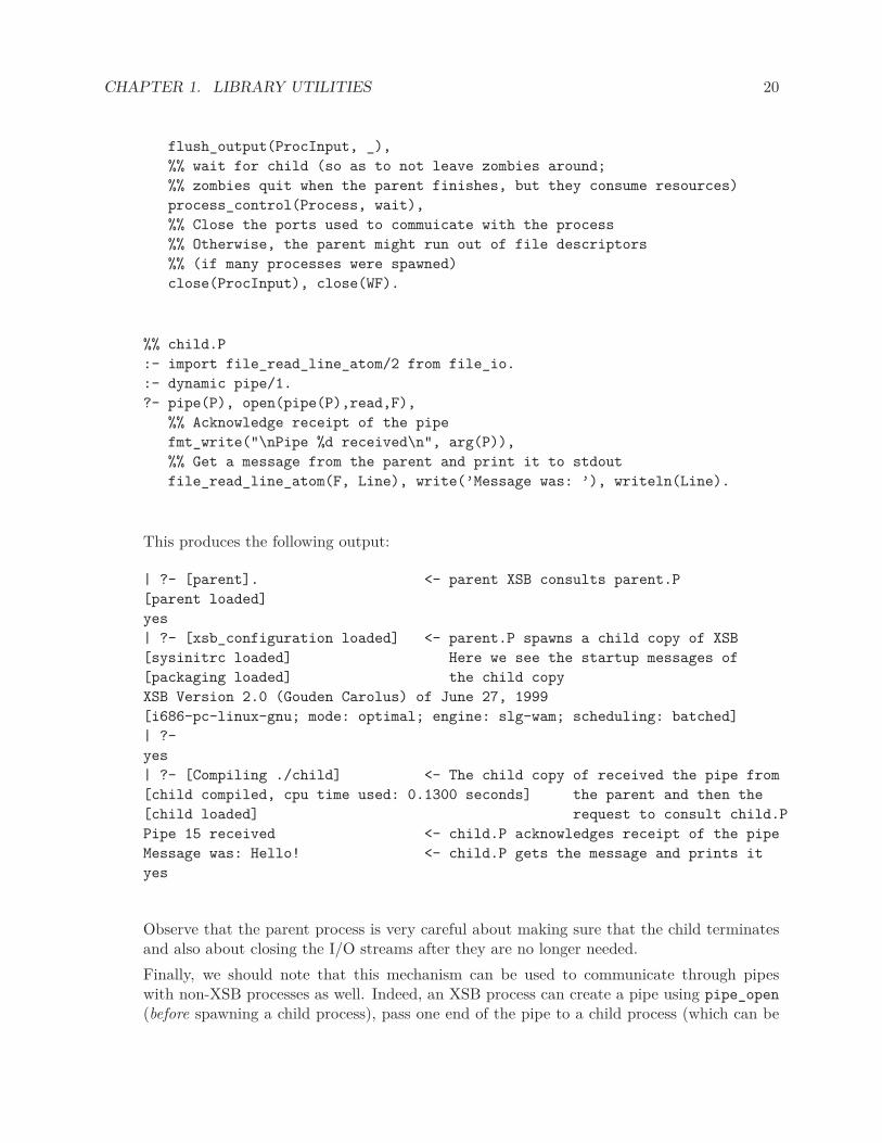
CHAPTER 1. LIBRARY UTILITIES 20
flush_output(ProcInput, _),
%% wait for child (so as to not leave zombies around;
%% zombies quit when the parent finishes, but they consume resources)
process_control(Process, wait),
%% Close the ports used to commuicate with the process
%% Otherwise, the parent might run out of file descriptors
%% (if many processes were spawned)
close(ProcInput), close(WF).
%% child.P
:- import file_read_line_atom/2 from file_io.
:- dynamic pipe/1.
?- pipe(P), open(pipe(P),read,F),
%% Acknowledge receipt of the pipe
fmt_write("\nPipe %d received\n", arg(P)),
%% Get a message from the parent and print it to stdout
file_read_line_atom(F, Line), write(’Message was: ’), writeln(Line).
This produces the following output:
| ?- [parent]. <- parent XSB consults parent.P
[parent loaded]
yes
| ?- [xsb_configuration loaded] <- parent.P spawns a child copy of XSB
[sysinitrc loaded] Here we see the startup messages of
[packaging loaded] the child copy
XSB Version 2.0 (Gouden Carolus) of June 27, 1999
[i686-pc-linux-gnu; mode: optimal; engine: slg-wam; scheduling: batched]
| ?-
yes
| ?- [Compiling ./child] <- The child copy of received the pipe from
[child compiled, cpu time used: 0.1300 seconds] the parent and then the
[child loaded] request to consult child.P
Pipe 15 received <- child.P acknowledges receipt of the pipe
Message was: Hello! <- child.P gets the message and prints it
yes
Observe that the parent process is very careful about making sure that the child terminatesand also about closing the I/O streams after they are no longer needed.
Finally, we should note that this mechanism can be used to communicate through pipeswith non-XSB processes as well. Indeed, an XSB process can create a pipe using pipe_open
(before spawning a child process), pass one end of the pipe to a child process (which can be

CHAPTER 1. LIBRARY UTILITIES 21
a C program), and use open/3 to convert the other end of the pipe to an XSB stream. TheC program, of course, does not need open/3, since it can use the pipe file handle directly.Likewise, a C program can spawn off an XSB process and pass it one end of a pipe. The XSBchild-process can then convert this pipe fd to a file using fd2iostream and then talk to theparent C program.
fd2iostream(+Pipe, -IOstream)
Take a file descriptor and convert it to an XSB I/O stream. This predicate should be usedonly for user-defined I/O. Otherwise, use open/{3,4} when possible.
1.7 Socket I/O
The XSB socket library defines a number of predicates for communication over BSD-style sockets.Most are modeled after and are interfaces to the socket functions with the same name. For detailedinformation on sockets, the reader is referred to the Unix man pages (another good source is UnixNetwork Programming, by W. Richard Stevens). Several examples of the use of the XSB socketsinterface can be found in the XSB/examples/ directory in the XSB distribution.
XSB supports two modes of communication via sockets: stream-oriented and message-oriented.In turn, stream-oriented communication can be buffered or character-at-a-time.
To use buffered stream-oriented communication, system socket handles must be converted toXSB I/O streams using fd2iostream/2. In these stream-oriented communication, messages haveno boundaries, and communication appears to the processes as reading and writing to a file. Atpresent, buffered stream-oriented communication works under Unix only.
Character-at-a-time stream communication is accomplished using the primitives socket_put/3
and socket_get0/3. These correspond to the usual Prolog put/1 and get0/1 I/O primitives.
In message-oriented communication, processes exchange messages that have well-defined bound-aries. The communicating processes use socket_send/3 and socket_recv/3 to talk to each other.XSB messages are represented as strings where the first four bytes (sizeof(int)) is an integer(represented in the binary network format — see the functions htonl and ntohl in socket docu-mentation) and the rest is the body of the message. The integer in the header represents the lengthof the message body.
Effort has been made to make the socket interface thread-safe; however in Version 3.3, calls tothe XSB socket interface go through a single mutex, and may cause contention if many threadsseek to concurrently use sockets.
We now describe the XSB socket interface. All predicates below must be imported from themodule socket. Note that almost all predicates have the last argument that unifies with the errorcode returned from the corresponding socket operation. This argument is explained separately.
General socket calls. These are used to open/close sockets, to establish connections, and setspecial socket options.

CHAPTER 1. LIBRARY UTILITIES 22
socket(-Sockfd, ?ErrorCode)
A socket Sockfd in the AF_INET domain is created. (The AF_UNIX domain is not yetimplemented). Sockfd is bound to a small integer, called socket descriptor or socket handle.
socket_set_option(+Sockfd,+OptionName,+Value)
Set socket option. At present, only the linger option is supported. “Lingering” is a situationwhen a socket continues to live after it was shut down by the owner. This is used in orderto let the client program that uses the socket to finish reading or writing from/to the socket.Value represents the number of seconds to linger. The value -1 means do not linger at all.
socket_close(+Sockfd, ?ErrorCode)
Sockfd is closed. Sockets used in socket_connect/2 should not be closed by socket_close/1
as they will be closed when the corresponding stream is closed.
socket_bind(+Sockfd,+Port, ?ErrorCode)
The socket Sockfd is bound to the specified local port number.
socket_connect(+Sockfd,+Port,+Hostname,?ErrorCode)
The socket Sockfd is connected to the address (Hostname and Port). If socket_connect/4
terminates abnormally for any reason (connection refused, timeout, etc.), then XSb closesthe socket Sockfd automatically, because such a socket cannot be used according to the BSDsemantics. Therefore, it is always a good idea to check to the return code and reopen thesocket, if the error code is not SOCK_OK.
socket_listen(+Socket, +Length, ?ErrorCode)
The socket Sockfd is defined to have a maximum backlog queue of Length pending connec-tions.
socket_accept(+Sockfd,-SockOut, ?ErrorCode)
Block the caller until a connection attempt arrives. If the incoming queue is not empty,the first connection request is accepted, the call succeeds and returns a new socket, SockOut,which can be used for this new connection.
Buffered, message-based communication. These calls are similar to the recv and send callsin C, except that XSB wraps a higher-level message protocol around these low-level functions. Moreprecisely, socket_send/3 prepends a 4-byte field to each message, which indicates the length of themessage body. When socket_recv/3 reads a message, it first reads the 4-byte field to determinethe length of the message and then reads the remainder of the message.
All this is transparent to the XSB user, but you should know these details if you want to usethese details to communicate with external processes written in C and such. All this means thatthese external programs must implement the same protocol. The subtle point here is that differentmachines represent integers differently, so an integer must first be converted into the machine-independent network format using the functions htonl and ntohl provided by the socket library.For instance, to send a message to XSB, one must do something like this:
char *message, *msg_body;

CHAPTER 1. LIBRARY UTILITIES 23
unsigned int msg_body_len, network_encoded_len;
msg_body_len = strlen(msg_body);
network_encoded_len = (unsigned int) htonl((unsigned long int) msg_body_len);
memcpy((void *) message, (void *) &network_encoded_len, 4);
strcpy(message+4, msg_body);
To read a message sent by XSB, one can do as follows:
int actual_len;
char lenbuf[4], msg_buff;
unsigned int msglen, net_encoded_len;
actual_len = (long)recvfrom(sock_handle, lenbuf, 4, 0, NULL, 0);
memcpy((void *) &net_encoded_len, (void *) lenbuf, 4);
msglen = ntohl(net_encoded_len);
msg_buff = calloc(msglen+1, sizeof(char))); // check if this suceeded!!!
recvfrom(sock_handle, msg_buff, msglen, 0, NULL, 0);
If making the external processes follow the XSB protocol is not practical (because you did notwrite these programs), then you should use the character-at-a-time interface or, better, the bufferedstream-based interface both of which are described in this section. At present, however, the bufferedstream-based interface does not work on Windows.
socket_recv(+Sockfd,-Message, ?ErrorCode)
Receives a message from the connection identified by the socket descriptor Sockfd. BindsMessage to the message. socket_recv/3 provides a message-oriented interface. It under-stands message boundaries set by socket_send/3.
socket_send(+Sockfd,+Message, ?ErrorCode)
Takes a message (which must be an atom) and sends it through the connection specifiedby Sockfd. socket_send/3 provides message-oriented communication. It prepends a 4-byteheader to the message, which tells socket_recv/3 the length of the message body.
Stream-oriented, character-at-a-time interface. Internally, this interface uses the samesendto and recvfrom socket calls, but they are executed for each character separately. Thisinterface is appropriate when the message format is not known or when message boundaries aredetermined using special delimiters.
socket_get0/3 creates the end-of-file condition when it receives the end-of-file character CH_EOF_P
(a.k.a. 255) defined in char_defs.h (which must be included in the XSB program). C programsthat need to send an end-of-file character should send (char)-1.
socket_get0(+Sockfd, -Char, ?ErrorCode)
The equivalent of get0 for sockets.
CHAPTER 1. LIBRARY UTILITIES 24
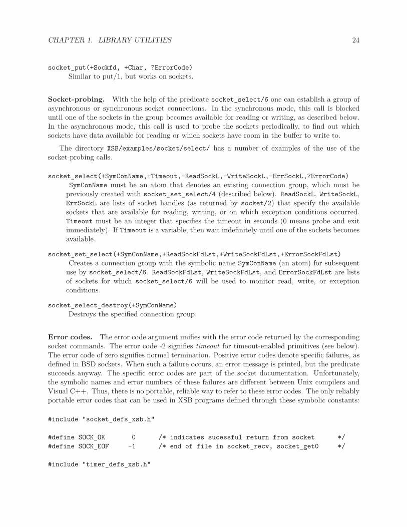
socket_put(+Sockfd, +Char, ?ErrorCode)
Similar to put/1, but works on sockets.
Socket-probing. With the help of the predicate socket_select/6 one can establish a group ofasynchronous or synchronous socket connections. In the synchronous mode, this call is blockeduntil one of the sockets in the group becomes available for reading or writing, as described below.In the asynchronous mode, this call is used to probe the sockets periodically, to find out whichsockets have data available for reading or which sockets have room in the buffer to write to.
The directory XSB/examples/socket/select/ has a number of examples of the use of thesocket-probing calls.
socket_select(+SymConName,+Timeout,-ReadSockL,-WriteSockL,-ErrSockL,?ErrorCode)
SymConName must be an atom that denotes an existing connection group, which must bepreviously created with socket_set_select/4 (described below). ReadSockL, WriteSockL,ErrSockL are lists of socket handles (as returned by socket/2) that specify the availablesockets that are available for reading, writing, or on which exception conditions occurred.Timeout must be an integer that specifies the timeout in seconds (0 means probe and exitimmediately). If Timeout is a variable, then wait indefinitely until one of the sockets becomesavailable.
socket_set_select(+SymConName,+ReadSockFdLst,+WriteSockFdLst,+ErrorSockFdLst)
Creates a connection group with the symbolic name SymConName (an atom) for subsequentuse by socket_select/6. ReadSockFdLst, WriteSockFdLst, and ErrorSockFdLst are listsof sockets for which socket_select/6 will be used to monitor read, write, or exceptionconditions.
socket_select_destroy(+SymConName)
Destroys the specified connection group.
Error codes. The error code argument unifies with the error code returned by the correspondingsocket commands. The error code -2 signifies timeout for timeout-enabled primitives (see below).The error code of zero signifies normal termination. Positive error codes denote specific failures, asdefined in BSD sockets. When such a failure occurs, an error message is printed, but the predicatesucceeds anyway. The specific error codes are part of the socket documentation. Unfortunately,the symbolic names and error numbers of these failures are different between Unix compilers andVisual C++. Thus, there is no portable, reliable way to refer to these error codes. The only reliablyportable error codes that can be used in XSB programs defined through these symbolic constants:
#include "socket_defs_xsb.h"
#define SOCK_OK 0 /* indicates sucessful return from socket */
#define SOCK_EOF -1 /* end of file in socket_recv, socket_get0 */
#include "timer_defs_xsb.h"

CHAPTER 1. LIBRARY UTILITIES 25
#define TIMEOUT_ERR -2 /* Timeout error code */
Timeouts. XSB socket interface allows the programer to specify timeouts for certain opera-tions. If the operations does not finish within the specified period of time, the operation isaborted and the corresponding predicate succeeds with the TIMEOUT_ERR error code. The fol-lowing primitives are timeout-enabled: socket_connect/4, socket_accept/3, socket_recv/3,socket_send/3, socket_get0/3, and socket_put/3. To set a timeout value for any of the aboveprimitives, the user should execute set_timer/1 right before the subgoal to be timed. Note thattimeouts are disabled after the corresponding timeout-enabled call completes or times out. There-fore, one must use set_timer/1 before each call that needs to be controlled by a timeout mechanism.
The most common use of timeouts is to either abort or retry the operation that times out. Forthe latter, XSB provides the sleep/1 primitive, which allows the program to wait for a few secondsbefore retrying.
The set_timer/1 and sleep/1 primitives are described below. They are standard predicatesand do not need to be explicitly imported.
set_timer(+Seconds)
Set timeout value. If a timer-enabled goal executes after this value is set, the clock beginsticking. If the goal does not finish in time, it succeeds with the error code set to TIMEOUT_ERR.The timer is turned off after the goal executes (whether timed out or not and whether itsucceeds or fails). This goal always succeeds.
Note that if the timer is not set, the timer-enabled goals execute “normally,” without timeouts.In particular, they might block (say, on socket_recv, if data is not available).
sleep(+Seconds)
Put XSB to sleep for the specified number of seconds. Execution resumes after the Seconds
number of seconds. This goal always succeeds.
Here is an example of the use of the timer:
:- compiler_options([xpp_on]).
#include "timer_defs_xsb.h"
?- set_timer(3), % wait for 3 secs
socket_recv(Sockfd, Msg, ErrorCode),
(ErrorCode == TIMEOUT_ERR
-> writeln(’Socket read timed out, retrying’),
try_again(Sockfd)
; write(’Data received: ’), writeln(Msg)
).
Apart from the above timer-enabled primitives, a timeout value can be given to socket_select/6
directly, as an argument.
CHAPTER 1. LIBRARY UTILITIES 26
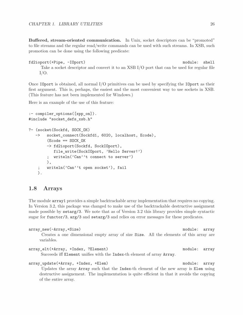
Buffered, stream-oriented communication. In Unix, socket descriptors can be “promoted”to file streams and the regular read/write commands can be used with such streams. In XSB, suchpromotion can be done using the following predicate:
fd2ioport(+Pipe, -IOport) module: shell
Take a socket descriptor and convert it to an XSB I/O port that can be used for regular fileI/O.
Once IOport is obtained, all normal I/O primitives can be used by specifying the IOport as theirfirst argument. This is, perhaps, the easiest and the most convenient way to use sockets in XSB.(This feature has not been implemented for Windows.)
Here is an example of the use of this feature:
:- compiler_options([xpp_on]).
#include "socket_defs_xsb.h"
?- (socket(Sockfd, SOCK_OK)
-> socket_connect(Sockfd1, 6020, localhost, Ecode),
(Ecode == SOCK_OK
-> fd2ioport(Sockfd, SockIOport),
file_write(SockIOport, ’Hello Server!’)
; writeln(’Can’’t connect to server’)
),
; writeln(’Can’’t open socket’), fail
).
1.8 Arrays
The module array1 provides a simple backtrackable array implementation that requires no copying.In Version 3.2, this package was changed to make use of the backtrackable destructive assignmentmade possible by setarg/3. We note that as of Version 3.2 this library provides simple syntacticsugar for functor/3, arg/3 and setarg/3 and relies on error messages for these predicates.
array_new(-Array,+Size) module: array
Creates a one dimensional empty array of size Size. All the elements of this array arevariables.
array_elt(+Array, +Index, ?Element) module: array
Succeeds iff Element unifies with the Index-th element of array Array.
array_update(+Array, +Index, +Elem) module: array
Updates the array Array such that the Index-th element of the new array is Elem usingdestructive assignement. The implementation is quite efficient in that it avoids the copyingof the entire array.
CHAPTER 1. LIBRARY UTILITIES 27
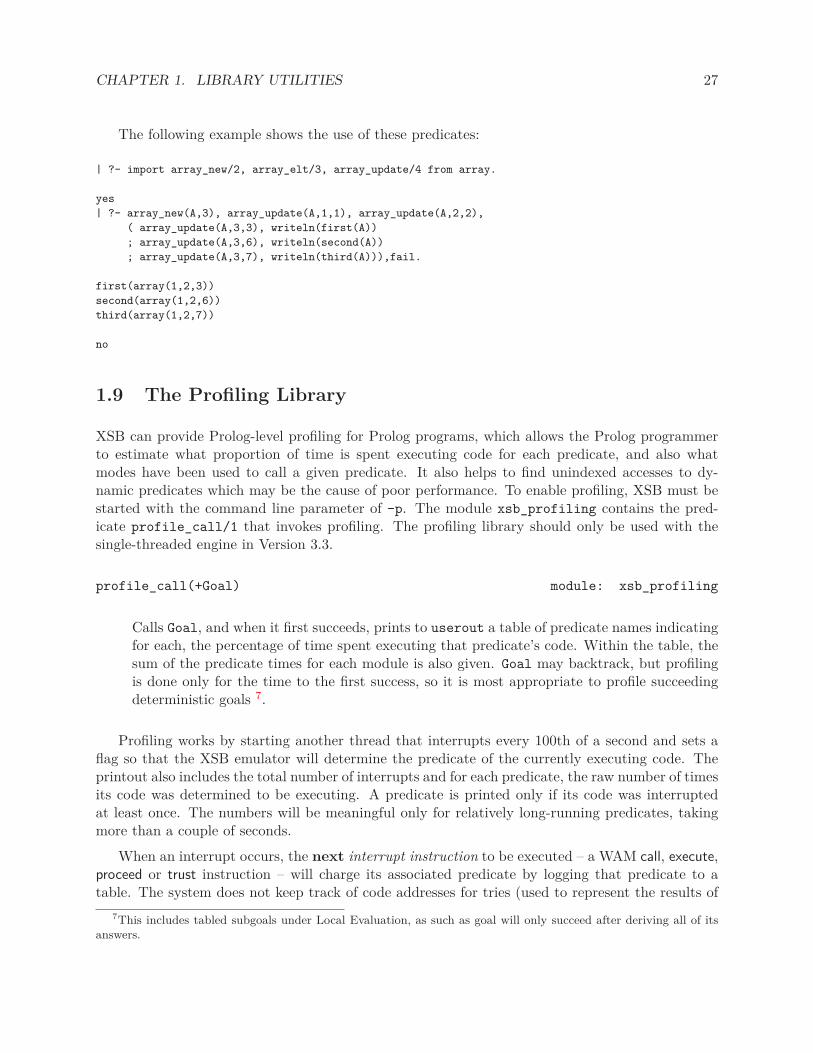
The following example shows the use of these predicates:
| ?- import array_new/2, array_elt/3, array_update/4 from array.
yes
| ?- array_new(A,3), array_update(A,1,1), array_update(A,2,2),
( array_update(A,3,3), writeln(first(A))
; array_update(A,3,6), writeln(second(A))
; array_update(A,3,7), writeln(third(A))),fail.
first(array(1,2,3))
second(array(1,2,6))
third(array(1,2,7))
no
1.9 The Profiling Library
XSB can provide Prolog-level profiling for Prolog programs, which allows the Prolog programmerto estimate what proportion of time is spent executing code for each predicate, and also whatmodes have been used to call a given predicate. It also helps to find unindexed accesses to dy-namic predicates which may be the cause of poor performance. To enable profiling, XSB must bestarted with the command line parameter of -p. The module xsb_profiling contains the pred-icate profile_call/1 that invokes profiling. The profiling library should only be used with thesingle-threaded engine in Version 3.3.
profile_call(+Goal) module: xsb_profiling
Calls Goal, and when it first succeeds, prints to userout a table of predicate names indicatingfor each, the percentage of time spent executing that predicate’s code. Within the table, thesum of the predicate times for each module is also given. Goal may backtrack, but profilingis done only for the time to the first success, so it is most appropriate to profile succeedingdeterministic goals 7.
Profiling works by starting another thread that interrupts every 100th of a second and sets aflag so that the XSB emulator will determine the predicate of the currently executing code. Theprintout also includes the total number of interrupts and for each predicate, the raw number of timesits code was determined to be executing. A predicate is printed only if its code was interruptedat least once. The numbers will be meaningful only for relatively long-running predicates, takingmore than a couple of seconds.
When an interrupt occurs, the next interrupt instruction to be executed – a WAM call, execute,proceed or trust instruction – will charge its associated predicate by logging that predicate to atable. The system does not keep track of code addresses for tries (used to represent the results of
7This includes tabled subgoals under Local Evaluation, as such as goal will only succeed after deriving all of itsanswers.
CHAPTER 1. LIBRARY UTILITIES 28
completed tables, and trie-indexed asserted code), so for some interrupts the associated executingpredicate cannot be determined. In these cases the interrupt is charged against an “unknown/?”pseudo-predicate, and this count is included in the output.
Profiling does not give the context from which the predicate is called, so you may want to makerenamed copies of basic predicates to use in particular circumstances to determine their times.
Predicates compiled with the “optimize” option may provide misleading results under profiling.Note that all system predicates (including those in basics) are compiled with the “optimize” option,by default. That option causes tail-recursive predicates to use a “jump” instruction rather thanan “execute” instruction to make the recursive call, and so an interrupt in such a loop will not becharged until the next interrupt instruction is executed. If much time is spent in the recursion, thismight not be for a long time, and the interrupt might ultimately be charged to another predicate.(If an interrupt has not been charged by the time of the next interrupt, it is lost.)
Profiling is currently available under Windows, Mac OS X, and Linux. However, for the profilingalgorithm to provide a good estimation, the thread that wakes and sets the interrupt flag must beof high priority and given the CPU when it wants it. Accordingly, the estimates may be better orworse depending on the scheduling strategy of a given platform 8.
The profiling module also provides support for determining when a dynamic predicate is invokedin a mode that isn’t supported by any index. The XSB programmer can set a flag that will causea message to be printed when a dynamic predicate is invoked, no index is applicable, and there aremore than 20 potentially matching clauses. See profile_unindexed_calls/1 below for details.
profile_mode_call(+Goal) module: xsb_profiling
Calls the goal Goal and constructs a table of the modes in which the predicate is called andthe number of times it is called in that mode. Modes are simply “b” for ground and “f” forvariable. Counts are kept in a table with entries of the form Pred(Md1,Md2,..,Mdn) wherePred is the name of the called predicate and the Mdi are either ’f’ or ’b’, indicating free orbound for the corresponding argument. The table can be printed using profile_mode_dump/0
and can be cleared using profile_mode_init/0.
profile_mode_dump module: xsb_profiling
Prints out the counts of calls in particular modes as accumulated usingprofile_mode_call(+Goal).
profile_mode_init module: xsb_profiling
Clears the table that accumulates counts of calls in particular modes (done byprofile_mode_call(+Goal).
8Windows and Mac OS X 10.6 provide good estimates. Some Linuxes however, do not charge about 20% of theirinterrupts due to thread scheduling issues. This loss of interrupts makes the profile estimate inefficient, but does notbias the estimate. We haven’t figured out how to get priority scheduling for interrupts on all machines, so if you wantprofiling to work more efficiently, maybe you can help figure out how to get appropriate scheduling.

CHAPTER 1. LIBRARY UTILITIES 29
profile_unindexed_calls(+Par) module: xsb_profiling
Sets the kind of unindexed profiling to perform. If Par is 0 no unindexed logging will bedone. (This is the default.) If Par is 1 each call to a dynamic predicate that cannot use anyindex (and would backtrack through more than 20 clauses) will generate a log message touserout. Each unindexed call to a predicate will be logged only once; after logging is done, thelog instruction is changed to a branch, so it will never produce another log message for thatdynamic code. If Par is 2, logging is done as for 1, except every unindexed call to any dynamicpredicate will be logged; i.e. the logging instruction is not changed after logging. If Par is apredicate specification (of the form Pred/Arity, Module:Pred/Arity, Term, or Module:Term),only unindexed calls to the indicated goal will be logged, and when each is logged a back-tracewill be printed. This allows the programmer to find the location of an unindexed call.
1.10 Gensym
The Gensym library provides a convenient way to generate unique integers or constants.
prepare(+Index) module: gensym
Sets the initial integer to be used for generation to Index. Thus, the command ?- prepare(0)
would cause the first call to gennum/1 to return 1. Index must be a non-negative integer.
gennum(-Var) module: gensym
Unifies Var with a new integer.
gensym(+Atom,-Var) module: gensym
Generates a new integer, and concatenates this integer with Atom, unifying the result withVar. For instance a call ?- gensym(foo,Var) might unify Var with foo32.
1.11 Random Number Generator
The following predicates are provided in module random to generate random numbers (both integersand floating numbers), based on the Wichmann-Hill Algorithm [30, 19]. The random numbergenerator is entirely portable, and does not require any calls to the operating system. As notedbelow, it does require 3 seeds, each of which must be an integer in a given range. These seeds arethread-specific: thus different threads may generate independent sequences of random numbers.
random(-Number) module: random
Binds Number to a random float in the interval [0.0, 1.0). Note that 1.0 will never begenerated.
random(+Lower,+Upper,-Number) module: random
Binds Number to a random integer in the interval [Lower,Upper) if Lower and Upper areintegers. Otherwise Number is bound to a random float between Lower and Upper. Upper willnever be generated.

CHAPTER 1. LIBRARY UTILITIES 30
getrand(?State) module: random
Tries to unify State with the term rand(X,Y,Z) where X,Y,and Z are integers describing thestate of the random generator.
setrand(rand(+X,+Y,+Z)) module: random
Sets the state of the random generator. X,Y, and Z must be integers in the ranges [1,30269),[1,30307), [1,30323), respectively.
datime_setrand module: random
This simple initialization utility sets the random seed triple based on a function of the currentday, hour, minute and second.
randseq(+K, +N, -RandomSeq) module: random
Generates a sequence of K unique integers chosen randomly in the range from 1 to N.RandomSeq is not returned in any particular order.
randset(+K, +N, -RandomSet) module: random
Generates an ordered set of K unique integers chosen randomly in the range from 1 to N. Theset is returned in reversed order, with the largest element first and the smallest last.
gauss(-G1,-G2) module: ramdom
Generates two random numbers that are normally distributed with mean 0 and standarddeviation 1. It uses the polar form of the Box-Muller transformation [5] of uniform randomvariables as generated by random/1.
weibull(K,Lambda,X) module: ramdom
Generates a random number for the Weibull distribution:
f(x; k, λ) =k
λ(x
λ)k−1e−(x/λ)h
based on the transformationx = λ(−ln(U))1/k
of a uniformly distributed ranom variable produce by random/1
exponential(K,X) module: ramdom
Generates a random number for the exponential distribution:
f(x; k, λ) =e−(x/λ)h
λ
based on the transformationx = λ(−ln(U))
of a uniformly distributed ranom variable produce by random/1. This is the same as theWeibull distribution with k = 1.

CHAPTER 1. LIBRARY UTILITIES 31
1.12 Loading Separated Files
A common file format uses comma separated values, the so-called csv files. The XSB module,proc_files, supports the loading of files in this, and similar, formats to define Prolog predicates.
load_csv(+FileName,+PredSpec) module: proc_files
load_csv/2 takes a file name and a predicate specification, and reads a csv-formatted fileinto memory, defining the indicated dynamic predicate. The simplest form of PredSpec isPredName/Arity. In this case the arity must equal the number of fields in the csv file, andthe predicate must be dynamic. Each line in the file will define one fact of the predicatePredName/Arity. Fields in the file enclosed in double quotes will be treated as single fields(and thus can contain commas and new-lines.) The dynamic predicate will be emptied beforethe facts from the file are added. Each field will be loaded as an atom (including fields thatcontain just integers.)
Alternatively, PredSpec may be of the form predName(TypeSpec1,...,TypeSpecN), wherepredName is the name of the dynamic predicate to be defined by the file contents, and eachTypeSpecI indicates the type of the corresponding field in the file. The permitted values ofTypeSpec are:
atom The corresponding field value will become an atom in the loaded fact.
integer The corresponding field value will be converted to an integer in the loaded fact.
float The corresponding field value will be converted to a float in the loaded fact.
term The corresponding field must contain a Prolog term in canonical form, and it will beconverted to that term in the loaded fact.
__ (A variable) Treated as atom.
load_dsv(+FileName,+PredSpec,+Options) module: proc_files
This predicate supports the loading of more general forms of files with value-separated fields.The FileName and PredSpec parameters are exactly as in load_csv/2, as described justabove. Options is a list of options. (With an empty list, load_dsv acts as load_csv/2.) Theoptions are:
separator=”Sep” which indicates that the character(s) Sep will be used as the field separator. There maybe one or more characters.
delimiter=”C” which indicates that the single character C will be used as the field delimiter (the defaultbeing “”””, and I’ve yet to find a situation in which I want to change it.)
titles which indicates that the first line of the file should be ignored and not contribute a factto the dynamic predicate.
CHAPTER 1. LIBRARY UTILITIES 32
1.13 Scanning in Prolog
Scanners, (sometimes called tokenizers) take an input string, usually in ASCII or similar format,and produce a scanned sequence of tokens. The requirements that various applications have forscanning differ in small but important ways – a character that is special to one application may bepart of the token of another; or some applications may want lower case text converted to upper-case test. The stdscan.P library provides a simple scanner written in XSB that can be configuredin several ways. While useful, this scanner is not intended to be as powerful as general-purposescanners such as lex or flex.
scan(+List,-Tokens) module: stdscan
Given as input a List of character codes, scan/2 scans this list producing a list of atomsconstituting the lexical tokens. Its parameters are set via set_scan_pars/1.
Tokens produced are either a sequence of letters and/or numbers or consist of a single specialcharacter (e.g. ( or )). Whitespaces may occur between tokens.
scan(+List,+FieldSeparator,-Tokens) module: stdscan
Given as input a List of character codes, along with a character code for a field separator,scan/3 scans this list producing a list of list of atoms constituting the lexical tokens ineach field. scan/3 thus can be used to scan tabular information. Its parameters are set viaset_scan_pars/1.
set_scan_pars(+List) module: stdscan
set_scan_pars(+List) is used to configure the tokenizer to a particular need. List is a listof parameters including the following:
• whitespace. The default action of the scanner is to return a list of tokens, with anywhitespace removed. If whitespace is a parameter, then the scanner returns the to-ken ” when it finds whitespace separating two tokens (unless the two tokens are lettersequences; since two letter sequences can be two tokens ONLY if they are separatedby whitespace, such an indication of whitespace would be redundant.) Including theparameter no_whitespace undoes the effect of previously including whitespace.
• upper_case The default action of the parser is to treat lowercase letter differently fromuppercase letters. This parameter should be set if conversion to uppercase should be donewhen producing a token that does not consist entirely of letters (e.g. one with mixedletters and digits). Including the parameter no_case undoes the effect of previouslyincluding upper_case.
• upper_case_in_lit The default action of the parser is to treat lowercase letter differ-ently from uppercase letters. This parameter should be set if conversion to uppercaseshould be done when producing a token that consists entirely of letters. Including theparameter no_case_in_lit undoes the effect of previously including upper_case.

CHAPTER 1. LIBRARY UTILITIES 33
• whitespace(Code) adds Code as a whitespace code. By default, all ASCII codes lessthan or equal to 32 are regarded as whitespace.
• letter(Code) adds Code as a letter constituting a token. By default, ASCII codes forcharacters a–z and A–Z are regarded as letters.
• special_char(Code) adds Code as a special character. By default, ASCII codes for thefollowing characters are regarded as special characters:
| { } [ ] " $ % & ’ ( ) * + , - . / : ; < = > ? @ \ ^ _ ~ ‘
get_scan_pars(-List) module: stdscan
get_scan_pars/1 returns a list of the currently active parameters.
1.14 XSB Lint
The xsb_lint_impexp.P file contains a simple tool to analyze import/exports and definitionsand uses of predicates. It tries to find possible inconsistencies, producing warnings when it findsthem and generating document_import/document_export declarations that might be useful. Itcan be used after a large multi-file, multi-module XSB program has been written to find possibleinconsistencies in (or interesting aspects of) how predicates are defined and used.
XSB source files that contain an export compiler directive are considered as modules. Predi-cates defined in modules, but not exported, are local to that module. When compiling a module,the XSB compiler generates useful warnings when predicates are used but not defined or definedbut not used. All predicates that are defined in source files that do not contain an export directiveare compiled to be defined in a global module, called usermod, and no warning messages are gen-erated. The user may add document_export and document_import compiler directives (exactlyanalogous to the export and import directives) to non-module source files. These directives areignored by the compiler for its compilation, but cause the define-use analysis to be done and anywarning messages to be issued, if appropriate. This allows a user to get the benefit of the define-useanalysis without using modules. (See Volume 1, Chapter 3 for more details.)
The xsb_lint_impexp utility processes both modules and regular XSB source files that containdocument_export statements. xsb_lint_impexp is not itself a module. To use it, [xsb_lint_impexp]
must be consulted, which will define the checkImpExps/{1,2} and add_libraries/1 predicatesin usermod.
add_libraries(+DirectoryNameList)
add_libraries/1 takes a list of directory names and adds them to the library_directory/1
predicate. This causes the XSB system to look for XSB source code files in these directories.To use checkImpExps/{1,2}, all the directories that contain files (or modules) referenced(recursively) in the files to be processed must be in the library_directory/1 predicate.This predicate can be used to add a number of directories at once.
checkImpExps(+Options,+FileNameList)
checkImpExps/1 reads all the XSB source files named in the list FileNameList, and all files
CHAPTER 1. LIBRARY UTILITIES 34
they reference (recursively), and produces a listing that describes properties of how theyreference predicates.
Options is a list of atoms (from the following list) indicating details of how checkImpExps
should work.
1. used_elsewhere: Print a warning message in the case of a predicate defined in a file,not used there, but used elsewhere (in a file in FileNameList). This can be useful tosee whether it might be better to move the predicate definition to another file, but itproduces many warnings for predicates in multi-use libraries.
2. unused: Print a warning message in the case of a predicate that is exported but neverused. This can be useful to see if predicate is not used anywhere, and thus could bedeleted. Again this produces many warnings for predicates in multi-use libraries.
3. all_files: By default, only predicates in files that contain a :- document_export or:- export declaration are processed. This option causes predicates of all files (andmodules) to be processed.
4. all_symbol_uses: Treat all non-predicate uses of symbols (even constants) as predicateuses for the purpose of generating imports.
5. no_symbol_uses: Don’t treat any non-predicate uses of symbols as predicate uses forthe purpose of generating imports.
We further explain the final two options, which allow the user to determine more preciselywhat uses of a symbol are considered as uses of it as the predicate symbol. All uses ofsymbols that appear in a “predicate context", i.e., in the body of a rule or in a meta-predicateargument position of a use of a meta-predicate, are considered uses of that predicate symbol.The default is also to allow nonconstant symbols appearing in any other context to also countas uses of that symbol as that predicate symbol. This is useful for programs that define theirown meta-predicates.
checkImpExps(+FileNameList)
checkImpExps/1 is currently equivalent to checkImpExps([],FileNameList).
1.15 Miscellaneous Predicates
term_hash(+Term,+HashSize,-HashVal) module: machine
Given an arbitrary Prolog term, Term, that is to be hashed into a table of HashSize buckets,this predicate returns a hash value for Term that is between 0 and HashSize -1.
pretty_print(+ClausePairs) module: pretty_print
pretty_print(+Stream,+ClausePairs) module: pretty_print
The input to pretty_print/1, ClausePairs, can be either a list of clause pairs or a singleclause pair. A clause pair is either a Prolog clause (or declaration) or a pair:

CHAPTER 1. LIBRARY UTILITIES 35
(Clause,Dict)
Where Dict is a list of the form A = V where V is a variable in Clause and A is the string tobe used to denote the variable 9.
By default, pretty_print/1 outputs atomic terms using writeq/1, but specialized outputcan be configured via asserting in usermod a term of the form
user_replacement_hook(Term,Call)
which will use Call to output an atomic literal A whenever A unifies with Term. For example,pretty printing weight constraints in XSB’s XASP package is done via the hook
user_replacement_hook(weight_constr(Term),output_weight_constr(Term))
which outputs a weight constraint in a (non-Prolog) syntax that is used by several ASPsystems.
1.16 Other Libraries
Not all XSB libraries are fully documented. We provide brief summaries of some of these otherlibraries.
1.16.1 Justification
By Hai-Feng Guo
Most Prolog debuggers, including XSB’s, are based on a mechanism that allows a user to tracethe evaluation of a goal by interrupting the evaluation at call, success, retry, or failure of varioussubgoals. While this has proved an excellent mechanism for evaluating SLD(NF) executions, it isdifficult at best to use such a mechanism during a tabled evaluation. This is because, unlike withSLD(NF), SLG requires answers to be returned to tabled subgoals at various times (depending onwhether batched or local evaluation is used), negative subgoals to be sometimes be delayed and/orsimplified, etc.
One approach to understanding tabled evaluation better is to abstract away the proceduralaspects of debugging and to use the tables produced by an evaluation to construct a justificationafter the evaluation has finished. The justification library does just this using algorithms describedin [14].
1.16.2 AVL Trees
By Mats Carlsson
9Thus the list of variable names returned by read_term/{2,3} can be used directly in Dict.

CHAPTER 1. LIBRARY UTILITIES 36
AVL trees provide a mechanism to maintain key value pairs so that loop up, insertion, anddeletion all have complexity O(log n). This library contains predicates to transform a sorted list toan AVL tree and back, along with predicates to manipulate the AVL trees.
1.16.3 Ordered Sets: ordsets.P
By Richard O’Keefe
(Summary from code documentation) ordset.P provides an XSB port of the widely used ordsetlibrary, whose summary we paraphrase here. In the ordset library, sets are represented by orderedlists with no duplicates. Thus {c,r,a,f,t} is represented as [a,c,f,r,t]. The ordering is defined bythe @< family of term comparison predicates, which is the ordering used by sort/2 and setof/3.The benefit of the ordered representation is that the elementary set operations can be done in timeproportional to the sum of the argument sizes rather than their product. Some of the unorderedset routines, such as member/2, length/2, or select/3 can be used unchanged.
1.16.4 Unweighted Graphs: ugraphs.P
By Mats Carlsson
XSB also includes a library for unweighted graphs. This library allows for the representationand manipulation of directed and non-directed unlabelled graphs, including predicates to find thetransitive closure of a graph, maximal paths, minimal paths, and other features. This libraryrepresents graphs as an ordered set of their edges and does not use tabling. As a result, it may beslower for large graphs than similar predicates based on a datalog representatoin of edges.
1.16.5 Heaps: heaps.P
By Richard O’Keefe
(Summary from code documentation). A heap is a labelled binary tree where the key of eachnode is less than or equal to the keys of its sons. The point of a heap is that we can keep onadding new elements to the heap and we can keep on taking out the minimum element. If thereare N elements total, the total time is O(Nlg(N)). If you know all the elements in advance, youare better off doing a merge-sort, but this file is for when you want to do say a best-first search,and have no idea when you start how many elements there will be, let alone what they are.
A heap is represented as a triple t(N, Free, Tree) where N is the number of elements in thetree, Free is a list of integers which specifies unused positions in the tree, and Tree is a tree madeof t terms for empty subtrees and t(Key,Datum,Lson,Rson) terms for the rest The nodes of thetree are notionally numbered like this:
1
2 3
4 6 5 7
8 12 10 14 9 13 11 15
CHAPTER 1. LIBRARY UTILITIES 37
.. .. .. .. .. .. .. .. .. .. .. .. .. .. .. ..
The idea is that if the maximum number of elements that have been in the heap so far is M ,and the tree currently has K elements, the tree is some subtreee of the tree of this form havingexactly M elements, and the Free list is a list of K −M integers saying which of the positions inthe M -element tree are currently unoccupied. This free list is needed to ensure that the cost ofpassing N elements through the heap is O(Nlg(M)) instead of O(NlgN). For M say 100 and Nsay 104 this means a factor of two.

Chapter 2
XSB-ODBC Interface
By Baoqiu Cui, Lily Dong, and David S. Warren 1.
2.1 Introduction
The XSB-ODBC interface is subsystem that allows XSB users to access databases through ODBCconnections. This is mostly of interest to Microsoft Windows users. The interface allows XSBusers to access data in any ODBC compliant database management system (DBMS). Using thisuniform interface, information in different DBMS’s can be accessed as though it existed as Prologfacts. The XSB-ODBC interface provides users with three levels of interaction: an SQL level, arelation level and a view level. The SQL level allows users to write explicit SQL statements to bepassed to the interface to retrieve data from a connected database. The relation level allows usersto declare XSB predicates that connect to individual tables in a connected database, and whichwhen executed support tuple-at-a-time retrieval from the base table. The view level allows users touse a complex XSB query, including conjunction, negation and aggregates, to specify a databasequery. A listing of the features that the XSB-ODBC interface provides is as follows:
• Concurrent access from multiple XSB processes to a single DBMS
• Access from a single XSB process to multiple ODBC DBMS’s
• Full data access and cursor transparency including support for
– Full data recursion through XSB’s tabling mechanism (depending on the capabilities ofthe underlying ODBC driver.
– Runtime type checking
– Automatic handling of NULL values for insertion, deletion and querying
• Full access to data source including
1This interface was partly based on the XSB-Oracle Interface by Hassan Davulcu, Ernie Johnson and TerranceSwift.
38

CHAPTER 2. XSB-ODBC INTERFACE 39
– Transaction support
– Cursor reuse for cached SQL statements with bind variables (thereby avoiding re-parsingand re-optimizing).
– Caching compiler generated SQL statements with bind variables and efficient cursormanagement for cached statements
• A powerful Prolog / SQL compiler based on [9].
• Full source code availability
• Independence from database schema by the relation level interface
• Performance as SQL by employing a view level
• No mode specification is required for optimized view compilation
We use the Hospital database as our example to illustrate the usage of XSB-ODBC interface inthis manual. We assume the basic knowledge of Microsoft ODBC interface and its ODBC adminis-trator throughout the text. Please refer to “Inside WindowsT M 95” (or more recent documentation)for information on this topic.
2.2 Using the Interface
The XSB-ODBC module is a module and as such exports the predicates it supports. In order touse any predicate defined below, it must be imported from odbc_call. For example, before youcan use the predicate to open a data source, you must include:
:- import odbc_open/3 from odbc_call.
2.2.1 Connecting to and Disconnecting from Data Sources
Assuming that the data source to be connected to is available, i.e. it has an entry in ODBC.INI filewhich can be checked by running Microsoft ODBC Administrator, it can be connected to in thefollowing way:
| ?- odbc_open(data_source_name, username, passwd).
If the connection is successfully made, the predicate invocation will succeed. This step isnecessary before anything can be done with the data sources since it gives XSB the opportunity toinitialize system resources for the session.
This is an executable predicate, but you may want to put it as a query in a file that declares adatabase interface and will be loaded.
To close the current session use:

CHAPTER 2. XSB-ODBC INTERFACE 40
| ?- odbc_close.
and XSB will give all the resources it allocated for this session back to the system.
If you are connecting to only one data source at a time, the predicates above are sufficient.However, if you want to connect to multiple data sources at the same time, you must use extendedversions of the predicates above. When connecting to multiple sources, you must give an atomicname to each source you want to connect to, and use that name whenever referring to that source.The names may be chosen arbitrarily but must be used consistently. The extended versions are:
| ?- odbc_open(data_source_name, username, passwd, connectionName).
and
| ?- odbc_close(connectionName).
A list of existing Data Source Names and descriptions can be obtained by backtracking throughodbc_data_sources/2. For example:
| ?- odbc_data_sources(DSN,DSNDescr).
DSN = mycdf
DSNDescr = MySQL driver;
DSN = mywincdf
DSNDescr = TDS driver (Sybase/MS SQL);
2.2.2 Accessing Tables in Data Sources Using SQL
There are several ways that can be used to extract information from or modify a table in a datasource. The most basic way is to use predicates that pass an SQL statement directly to the ODBCdriver. The basic call is:
| ?- odbc_sql(BindVals,SQLStmt,ResultRow).
where BindVals is a list of (ground) values that correspond to the parameter indicators in theSQL statement (the ’?’s); SQLStmt is an atom containing an SQL statement; and ResultRow is areturned list of values constituting a row from the result set returned by the SQL query. Thus fora select SQL statement, this call is nondeterministic, returning each retrieved row in turn.
The BindVals list should have a length corresponding to the number of parameters in thequery, in particular being the empty list ([]) if SQLStmt contains no ’?’s. If SQLStmt is not a selectstatement returning a result set, then ResultRow will be the empty list, and the call is deterministic.Thus this predicate can be used to do updates, DDL statements, indeed any SQL statement.
CHAPTER 2. XSB-ODBC INTERFACE 41
SQLStmt need not be an atom, but can be a (nested) list of atoms which flattens (and concate-nates) to form an SQL statement.
BindVals is normally a list of values of primitive Prolog types: atoms, integers, or floats.The values are converted to the types of the corresponding database fields. However, complexProlog values can also be stored in a database field. If a term of the form term(VAL) appearsin the BindVal list, then VAL (a Prolog term) will be written in canonical form (as produced bywrite_canonical) to the corresponding database field (which must be CHAR or BYTE). If a termof the form string(CODELIST) appears in BindVal, then CODELIST must be a list of ascii-codes (asproduced by atom_codes) and these codes will be converted to a CHAR or BYTE database type.
ResultRow for a select statement is normally a list of variables that will nondeterministically bebound to the values of the fields of the tuples returned by the execution of the select statement. TheProlog types of the values returned will be determined by the database types of the correspondingfields. A CHAR or BYTE database type will be returned as a Prolog atom; an INTEGER databasefield will be returned as a Prolog integer, and similarly for floats. However, the user can requestthat CHAR and BYTE database fields be returned as something other than an atom. If theterm string(VAR) appears in ResultRow, then the corresponding database field must be CHARor BYTE, and in this case, the variable VAR will be bound to the list of ascii-codes that make upthe database field. This allows an XSB programmer to avoid adding an atom to the atom tableunnecessarily. If the term term(VAR) appears in ResultRow, then the corresponding database fieldvalue is assumed to be a Prolog term in canonical form, i.e., can be read by read_canonical/1.The corresponding value will be converted into a Prolog term and bound to VAR. This allows aprogrammer to store complex Prolog terms in a database. Variables in such a term are local onlyto that term.
When connecting to multiple data sources, you should use the form:
| ?- odbc_sql(ConnectionName,BindVals,SQLStmt,ResultRow).
For example, we can define a predicate, get_test_name_price, which given a test ID, retrievesthe name and price of that test from the test table in the hospital database:
get_test_name_price(Id,Nam,Pri) :-
odbc_sql([Id],’SELECT TName,Price FROM Test WHERE TId = ?’, [Nam,Pri]).
The interface uses a cursor to retrieve this result and caches the cursor, so that if the samequery is needed in the future, it does not need to be re-parsed, and re-optimized. Thus, if thispredicate were to be called several times, the above form is more efficient than the following form,which must be parsed and optimized for each and every call:
get_test_name_price(Id,Nam,Pri) :-
odbc_sql([],[’SELECT TName,Price FROM Test WHERE TId = ’’’,Id,’’’’], [Nam,Pri]).
Note that to include a quote (’) in an atom, it must be represented by using two quotes.
There is also a predicate:
CHAPTER 2. XSB-ODBC INTERFACE 42
| ?- odbc_sql_cnt(ConnectionName,BindVals,SQLStmt,Count).
This predicate is very similar to odbc_slq/4 except that it can only be used for UPDATE,INSERT, and DELETE SQL statements. The first three arguments are just as in odbc_slq/4; thefourth must be a variable in which is returned the integer count of the number of rows affected bythe SQL operation.
2.2.3 Cursor Management
The XSB-ODBC interface is limited to using 100 open cursors. When XSB systems use databaseaccesses in a complicated manner, management of open cursors can be a problem due to thetuple-at-a-time access of databases from Prolog, and due to leakage of cursors through cuts andthrows. Often, it is more efficient to call the database through set-at-a-time predicates such asfindall/3, and then to backtrack through the returned information. For instance, the predicatefindall_odbc_sql/4 can be defined as:
findall_odbc_sql(ConnName,BindVals,SQLStmt,ResultRow):-
findall(Res,odbc_sql(ConnName,BindVals,SQLStmt,Res),Results),
member(ResultRow,Results).
As a convenience, therefore, the predicates findall_odbc_sql/3 and findall_odbc_sql/4 aredefined in the ODBC interface.
2.2.4 Accessing Tables in Data Sources through the Relation Level
While all access to a database is possible using SQL as described above, the XSB-ODBC interfacesupports higher-level interaction for which the user need not know or write SQL statements; thatis done as necessary by the interface. With the relation level interface, users can simply declarea predicate to access a table and the system generates the necessary underlying code, generatingspecialized code for each mode in which the predicate is called.
To declare a predicate to access a database table, a user must use the odbc_import/2 interfacepredicate.
The syntax of odbc_import/2 is as follows:
| ?- odbc_import(’TableName’(’FIELD1’, ’FIELD2’, ..., ’FIELDn’), ’PredicateName’).
where ’TableName’ is the name of the database table to be accessed and ’PredicateName’ is thename of the XSB predicate through which access will be made. ’FIELD1’, ’FIELD2’, ... , ’FIELDn’
are the exact attribute names(case sensitive) as defined in the database table schema. The chosencolumns define the view and the order of arguments for the database predicate ’PredicateName’.
For example, to create a link to the Test table through the ’test’ predicate:
CHAPTER 2. XSB-ODBC INTERFACE 43
| ?- odbc_import(’Test’(’TId’,’TName’,’Length’,’Price’),test).
yes
When connecting to multiple data sources, you should use the form:
| ?- odbc_import(ConnectionName,
’TableName’(’FIELD1’, ’FIELD2’, ..., ’FIELDn’),
’PredicateName’).
2.2.5 Using the Relation Level Interface
Once the links between tables and predicates have been successfully established, information canthen be extracted from these tables using the corresponding predicates. Continuing from the aboveexample, now rows from the table Test can be obtained:
| ?- test(TId, TName, L, P).
TId = t001
TName = X-Ray
L = 5
P = 100
Backtracking can then be used to retrieve the next row of the table Test.
Records with particular field values may be selected in the same way as in Prolog; no modespecification for database predicates is required. For example:
| ?- test(TId, ’X-Ray’, L, P).
will automatically generate the query:
SELECT rel1.TId, rel1.TName, rel1.Length, rel1.Price
FROM Test rel1
WHERE rel1.TName = ?
and
| ?- test(’NULL’(_), ’X-Ray’, L, P).
generates: (See Section 2.2.6)
SELECT NULL , rel1.TName, rel1.Length, rel1.Price
FROM Test rel1
WHERE rel1.TId IS NULL AND rel1.TName = ?

CHAPTER 2. XSB-ODBC INTERFACE 44
During the execution of this query the bind variable ? will be bound to the value ’X-Ray’.
Of course, the same considerations about cursors noted in Section 2.2.3 apply to the relation-level interface. Accordingly, the ODBC interface also defines the predicate odbc_import/4 whichallows the user to specify that rows are to be fetched through findall/3. For example, the call
odbc_import(’Test’(’TId’,’TName’,’Length’,’Price’),test,[findall(true)]).
will behave as described above but will make all database calls through findall/3 and return rowsby backtracking through a list rather than maintaining open cursors.
Also as a courtesy to Quintus Prolog users we have provided compatibility support for somePRODBI predicates which access tables at a relational level 2.
| ?- odbc_attach(PredicateName, table(TableName)).
eg. invoke
| ?- odbc_attach(test2, table(’Test’)).
and then execute
| ?- test2(TId, TName, L, P).
to retrieve the rows.
2.2.6 Handling NULL values
The interface treats NULL’s by introducing a single valued function ’NULL’/1 whose single valueis a unique (Skolem) constant. For example a NULL value may be represented by
’NULL’(null123245)
Under this representation, two distinct NULL values will not unify. On the other hand, the searchcondition IS NULL Field can be represented in XSB as Field = ’NULL’(_)
Using this representation of NULL’s the following protocol for queries and updates is established.
Queries
| ?- dept(’NULL’(_),_,_).
Generates the query:
2This predicate is obsolescent and odbc_import/{2,3,4} should be used instead.

CHAPTER 2. XSB-ODBC INTERFACE 45
SELECT NULL , rel1.DNAME , rel1.LOC
FROM DEPT rel1
WHERE rel1.DEPTNO IS NULL;
Hence, ’NULL’(_) can be used to retrieve rows with NULL values at any field.
’NULL’/1 fails the predicate whenever it is used with a bound argument.
| ?- dept(’NULL’(null2745),_,_). → fails always.
Query Results
When returning NULL’s as field values, the interface returns NULL/1 function with a unique integerargument serving as a skolem constant.
Notice that the above guarantees the expected semantics for the join statements. In the followingexample, even if Deptno is NULL for some rows in emp or dept tables, the query still evaluates thejoin successfully.
| ?- emp(Ename,_,_,_,Deptno),dept(Deptno,Dname,Loc)..
Inserts
To insert rows with NULL values you can use Field = ’NULL’(_) or Field = ’NULL’(null2346).For example:
| ?- emp_ins(’NULL’(_), ...). → inserts a NULL value for ENAME
| ?- emp_ins(’NULL’(’bound’), ...) → inserts a NULL value for ENAME.
Deletes
To delete rows with NULL values at any particular FIELD use Field = ’NULL’(_), ’NULL’/1 witha free argument. When ’NULL’/1 ’s argument is bound it fails the delete predicate always. Forexample:
| ?- emp_del(’NULL’(_), ..). → adds ENAME IS NULL to the generated SQL
statement
| ?- emp_del(’NULL’(’bound’), ...). → fails always
The reason for the above protocol is to preserve the semantics of deletes, when some freearguments of a delete predicate get bound by some preceding predicates. For example in thefollowing clause, the semantics is preserved even if the Deptno field is NULL for some rows.
| ?- emp(_,_,_,_,Deptno), dept_del(Deptno).
CHAPTER 2. XSB-ODBC INTERFACE 46
2.2.7 The View Level Interface
The view level interface can be used to define XSB queries which include only imported databasepredicates (by using the relation level interface) described above and aggregate predicates (definedbelow). When these queries are invoked, they are translated into complex database queries, whichare then executed taking advantage of the query processing ability of the DBMS.
One can use the view level interface through the predicate odbc_query/2:
| ?- odbc_query(’QueryName’(ARG1, ..., ARGn), DatabaseGoal).
All arguments are standard XSB terms. ARG1, ARG2, ..., ARGn define the attributes to be retrievedfrom the database, while DatabaseGoal is an XSB goal (i.e. a possible body of a rule) that definesthe selection restrictions and join conditions.
The compiler is a simple extension of [9] which generates SQL queries with bind variables andhandles NULL values as described in Section 2.2.6. It allows negation, the expression of arithmeticfunctions, and higher-order constructs such as grouping, sorting, and aggregate functions.
Database goals are translated according to the following rules from [9]:
• Disjunctive goals translate to distinct SQL queries connected through the UNION operator.
• Goal conjunctions translate to joins.
• Negated goals translate to negated EXISTS subqueries.
• Variables with single occurrences in the body are not translated.
• Free variables translate to grouping attributes.
• Shared variables in goals translate to equi-join conditions.
• Constants translate to equality comparisons of an attribute and the constant value.
• Nulls are translated to IS NULL conditions.
For more examples and implementation details see [9].
In the following, we show the definition of a simple join view between the two database predicatesRoom and Floor.
Assuming the declarations:
| ?- odbc_import(’Room’(’RoomNo’,’CostPerDay’,’Capacity’,’FId’),room).
| ?- odbc_import(’Floor’(’FId’,’’,’FName’),floor).
use

CHAPTER 2. XSB-ODBC INTERFACE 47
| ?- odbc_query(query1(RoomNo,FName),
(room(RoomNo,_,_,FId),floor(FId,_,FName))).
yes
| ?- query1(RoomNo,FloorName).
Prolog/SQL compiler generates the SQL statement:
SELECT rel1.RoomNo , rel2.FName FROM Room rel1 , Floor rel2
WHERE rel2.FId = rel1.FId;
Backtracking can then be used to retrieve the next row of the view.
| ?- query1(’101’,’NULL’(_)).
generates the SQL statement:
SELECT rel1.RoomNo, NULL
FROM Room rel1 , Floor rel2
WHERE rel1.RoomId = ? AND rel2.FId = rel1.FId AND rel2.FName IS NULL;
The view interface also supports aggregate functions such as sum, avg, count, min and max.For example
| ?- odbc_import(’Doctor’(’DId’, ’FId’, ’DName’,’PhoneNo’,’ChargePerMin’),doctor).
yes
| ?- odbc_query(avgchargepermin(X),
(X is avg(ChargePerMin, A1 ^ A2 ^ A3 ^ A4 ^
doctor(A1,A2, A3,A4,ChargePerMin)))).
yes
| ?- avgchargepermin(X).
SELECT AVG(rel1.ChargePerMin)
FROM doctor rel1;
X = 1.64
yes
A more complicated example is the following:
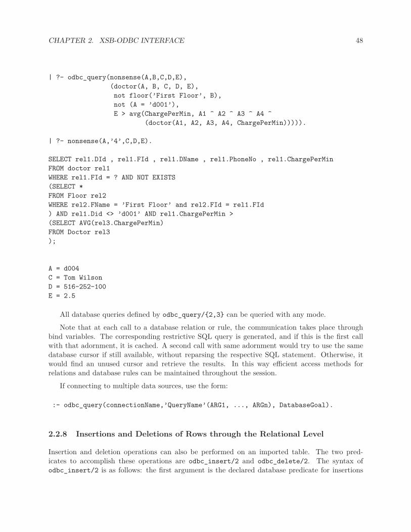
CHAPTER 2. XSB-ODBC INTERFACE 48
| ?- odbc_query(nonsense(A,B,C,D,E),
(doctor(A, B, C, D, E),
not floor(’First Floor’, B),
not (A = ’d001’),
E > avg(ChargePerMin, A1 ^ A2 ^ A3 ^ A4 ^
(doctor(A1, A2, A3, A4, ChargePerMin))))).
| ?- nonsense(A,’4’,C,D,E).
SELECT rel1.DId , rel1.FId , rel1.DName , rel1.PhoneNo , rel1.ChargePerMin
FROM doctor rel1
WHERE rel1.FId = ? AND NOT EXISTS
(SELECT *
FROM Floor rel2
WHERE rel2.FName = ’First Floor’ and rel2.FId = rel1.FId
) AND rel1.Did <> ’d001’ AND rel1.ChargePerMin >
(SELECT AVG(rel3.ChargePerMin)
FROM Doctor rel3
);
A = d004
C = Tom Wilson
D = 516-252-100
E = 2.5
All database queries defined by odbc_query/{2,3} can be queried with any mode.
Note that at each call to a database relation or rule, the communication takes place throughbind variables. The corresponding restrictive SQL query is generated, and if this is the first callwith that adornment, it is cached. A second call with same adornment would try to use the samedatabase cursor if still available, without reparsing the respective SQL statement. Otherwise, itwould find an unused cursor and retrieve the results. In this way efficient access methods forrelations and database rules can be maintained throughout the session.
If connecting to multiple data sources, use the form:
:- odbc_query(connectionName,’QueryName’(ARG1, ..., ARGn), DatabaseGoal).
2.2.8 Insertions and Deletions of Rows through the Relational Level
Insertion and deletion operations can also be performed on an imported table. The two pred-icates to accomplish these operations are odbc_insert/2 and odbc_delete/2. The syntax ofodbc_insert/2 is as follows: the first argument is the declared database predicate for insertions

CHAPTER 2. XSB-ODBC INTERFACE 49
and the second argument is some imported data source relation. The second argument can be de-clared with some of its arguments bound to constants. For example after Room is imported throughodbc_import:
|?- odbc_import(’Room’(’RoomNo’,’CostPerDay’,’Capacity’,’FId’), room).
yes
Now we can do
| ?- odbc_insert(room_ins(A1,A2,A3),(room(A1,A2,A3,’3’))).
yes
| ?- room_ins(’306’,’NULL’(_),2).
yes
This will insert the row: (’306’,NULL, 2,’3’) into the table Room. Note that any call to room_ins/7
should have all its arguments bound.
See Section 2.2.6) for information about NULL value handling.
The first argument of odbc_delete/2 predicate is the declared delete predicate and the secondargument is the imported data source relation with the condition for requested deletes, if any. Thecondition is limited to simple comparisons. For example assuming Room/3 has been imported asabove:
| ?- odbc_delete(room_del(A), (room(’306’,A,B,C), A > 2)).
yes
After this declaration you can use:
| ?- room_del(3).
to generate the SQL statement:
DELETE From Room rel1
WHERE rel1.RoomNo = ’306’ AND rel1.CostPerDay = ? AND ? > 2
;
Note that you have to commit your inserts or deletes to tables to make them permanent. (Seesection 2.2.11).

CHAPTER 2. XSB-ODBC INTERFACE 50
These predicates also have the form in which an additional first argument indicates a connection,for use with multiple data sources.
Also, some ODBC drivers have been found that do not accept the form of SQL generated fordeletes. In these cases, you must use the lower-level interface: odbc_sql.
2.2.9 Access to Data Dictionaries
The following utility predicates provide users with tools to access data dictionaries 3. A briefdescription of these predicates is as follows:
odbc_show_schema(accessible(Owner)) Shows the names of all accessible tables that areowned by Owner. (This list can be long!) If Owner is a variable, all tables will be shown,grouped by owner.
odbc_show_schema(user) Shows just those tables that belongs to user.
odbc_show_schema(tuples(’Table’)) Shows all rows of the database table named ’Table’.
odbc_show_schema(arity(’Table’)) The number of fields in the table ’Table’.
odbc_show_schema(columns(’Table’)) The field names of a table.
For retrieving above information use:
• odbc_get_schema(accessible(Owner),List)
• odbc_get_schema(user,List)
• odbc_get_schema(arity(’Table’),List)
• odbc_get_schema(columns(’Table’),List)
The results of above are returned in List as a list.
2.2.10 Other Database Operations
odbc_create_table(’TableName’,’FIELDs’) FIELDS is the field specification as in SQL.
eg. odbc_create_table(’MyTable’, ’Col1 NUMBER,
Col2 TEXT(50),
Col3 TEXT(13)’).
odbc_create_index(’TableName’,’IndexName’, index(_,Fields)) Fields is the list of columnsfor which an index is requested. For example:
3Users of Quintus Prolog may note that these predicates are all PRODBI compatible.
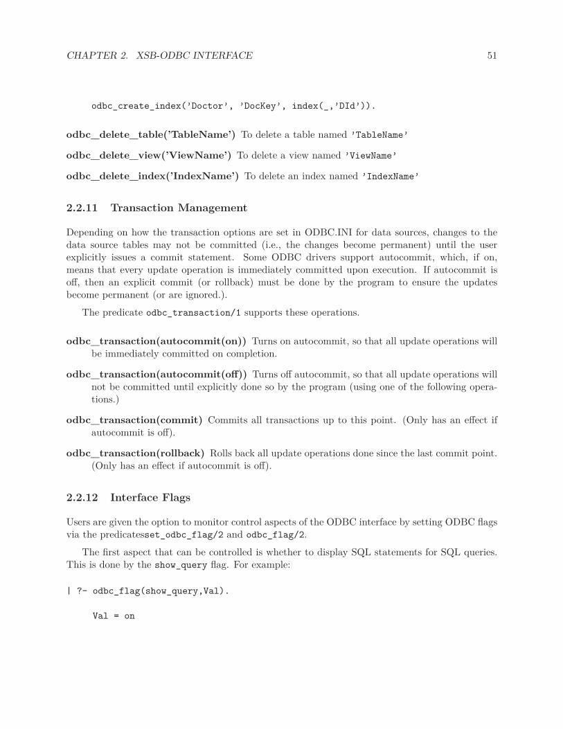
CHAPTER 2. XSB-ODBC INTERFACE 51
odbc_create_index(’Doctor’, ’DocKey’, index(_,’DId’)).
odbc_delete_table(’TableName’) To delete a table named ’TableName’
odbc_delete_view(’ViewName’) To delete a view named ’ViewName’
odbc_delete_index(’IndexName’) To delete an index named ’IndexName’
2.2.11 Transaction Management
Depending on how the transaction options are set in ODBC.INI for data sources, changes to thedata source tables may not be committed (i.e., the changes become permanent) until the userexplicitly issues a commit statement. Some ODBC drivers support autocommit, which, if on,means that every update operation is immediately committed upon execution. If autocommit isoff, then an explicit commit (or rollback) must be done by the program to ensure the updatesbecome permanent (or are ignored.).
The predicate odbc_transaction/1 supports these operations.
odbc_transaction(autocommit(on)) Turns on autocommit, so that all update operations willbe immediately committed on completion.
odbc_transaction(autocommit(off)) Turns off autocommit, so that all update operations willnot be committed until explicitly done so by the program (using one of the following opera-tions.)
odbc_transaction(commit) Commits all transactions up to this point. (Only has an effect ifautocommit is off).
odbc_transaction(rollback) Rolls back all update operations done since the last commit point.(Only has an effect if autocommit is off).
2.2.12 Interface Flags
Users are given the option to monitor control aspects of the ODBC interface by setting ODBC flagsvia the predicatesset_odbc_flag/2 and odbc_flag/2.
The first aspect that can be controlled is whether to display SQL statements for SQL queries.This is done by the show_query flag. For example:
| ?- odbc_flag(show_query,Val).
Val = on
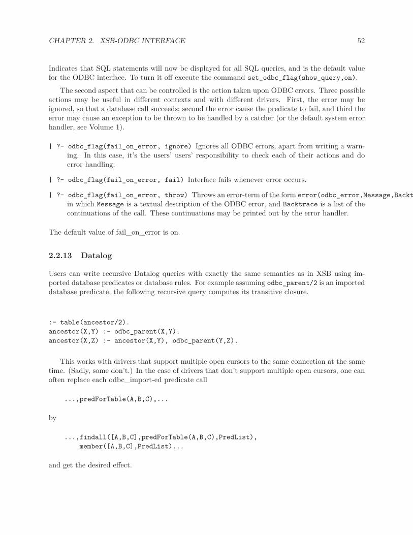
CHAPTER 2. XSB-ODBC INTERFACE 52
Indicates that SQL statements will now be displayed for all SQL queries, and is the default valuefor the ODBC interface. To turn it off execute the command set_odbc_flag(show_query,on).
The second aspect that can be controlled is the action taken upon ODBC errors. Three possibleactions may be useful in different contexts and with different drivers. First, the error may beignored, so that a database call succeeds; second the error cause the predicate to fail, and third theerror may cause an exception to be thrown to be handled by a catcher (or the default system errorhandler, see Volume 1).
| ?- odbc_flag(fail_on_error, ignore) Ignores all ODBC errors, apart from writing a warn-ing. In this case, it’s the users’ users’ responsibility to check each of their actions and doerror handling.
| ?- odbc_flag(fail_on_error, fail) Interface fails whenever error occurs.
| ?- odbc_flag(fail_on_error, throw) Throws an error-term of the form error(odbc_error,Message,Backtrace)
in which Message is a textual description of the ODBC error, and Backtrace is a list of thecontinuations of the call. These continuations may be printed out by the error handler.
The default value of fail_on_error is on.
2.2.13 Datalog
Users can write recursive Datalog queries with exactly the same semantics as in XSB using im-ported database predicates or database rules. For example assuming odbc_parent/2 is an importeddatabase predicate, the following recursive query computes its transitive closure.
:- table(ancestor/2).
ancestor(X,Y) :- odbc_parent(X,Y).
ancestor(X,Z) :- ancestor(X,Y), odbc_parent(Y,Z).
This works with drivers that support multiple open cursors to the same connection at the sametime. (Sadly, some don’t.) In the case of drivers that don’t support multiple open cursors, one canoften replace each odbc_import-ed predicate call
...,predForTable(A,B,C),...
by
...,findall([A,B,C],predForTable(A,B,C),PredList),
member([A,B,C],PredList)...
and get the desired effect.

CHAPTER 2. XSB-ODBC INTERFACE 53
2.3 Error messages
ERR - DB: Connection failed For some reason the attempt to connect to data source failed.
• Diagnosis: Try to see if the data source has been registered with Microsoft ODBCAdministrator, the username and password are correct and MAXCURSORNUM is notset to a very large number.
ERR - DB: Parse error The SQL statement generated by the Interface or the first argument toodbc_sql/1 or odbc_sql_select/2 can not be parsed by the data source driver.
• Diagnosis: Check the SQL statement. If our interface generated the erroneous statementplease contact us at [email protected].
ERR - DB: No more cursors left Interface run out of non-active cursors either because of aleak or no more free cursors left.
• Diagnosis: System fails always with this error. odbc_transaction(rollback) or odbc_transaction(commit)should resolve this by freeing all cursors.
ERR - DB: FETCH failed Normally this error should not occur if the interface running prop-erly.
• Diagnosis: Please contact us at [email protected]
2.4 Notes on specific ODBC drivers
MyODBC The ODBC driver for MySQL is called MyODBC, and it presents some partic-ularities that should be noted.
First, MySQL, as of version 3.23.55, does not support strings of length greater than255 characters. XSB’s ODBC interface has been updated to allow the use of the BLOBdatatype to encode larger strings.
More importantly, MyODBC implements SQLDescribeCol such that, by default, it re-turns actual lengths of columns in the result table, instead of the formal lengths in thetables. For example, suppose you have, in table A, a field f declared as “VARCHAR(200)”. Now, you create a query of the form “SELECT f FROM A WHERE ...” If,in the result set, the largest size of f is 52, that’s the length that SQLDescribeCol willreturn. This breaks XSB’s caching of query-related data-structures. In order to preventthis behavior, you should configure your DSN setup so that you pass “Option=1” toMyODBC.

Chapter 3
The New XSB-Database Interface
By Saikat Mukherjee, Michael Kifer and Hui Wan
3.1 Introduction
The XSB-DB interface is a package that allows XSB users to access databases through variousdrivers. Using this interface, information in different DBMSs can be accessed by SQL queries.The interface defines Prolog predicates which makes it easy to connect to databases, query them,and disconnect from the databases. Central to the concept of a connection to a database is thenotion of a connection handle. A connection handle describes a particular connection to a database.Similar to a connection handle is the notion of a query handle which describes a particular querystatement. As a consequence of the handles, it is possible to open multiple database connections (tothe same or different databases) and keep alive multiple queries (again from the same or differentconnections). The interface also supports dynamic loading of drivers. As a result, it is possible toquery databases using different drivers concurrently 1.
Currently, this package provides drivers for ODBC, a native MySQL driver, and a driver forthe embedded MySQL server.
3.2 Configuring the Interface
Generally, each driver has to be configured separately, but if the database packages such as ODBC,MySql, etc., are installed in standard places then the XSB configuration mechanism will do the jobautomatically.
Under Windows, first make sure that XSB is configured and built correctly for Windows, andthat it runs. As part of that building process, the command
makexsb_wind
1In Version 3.3, this package has not been ported to the multi-threaded engine.
54
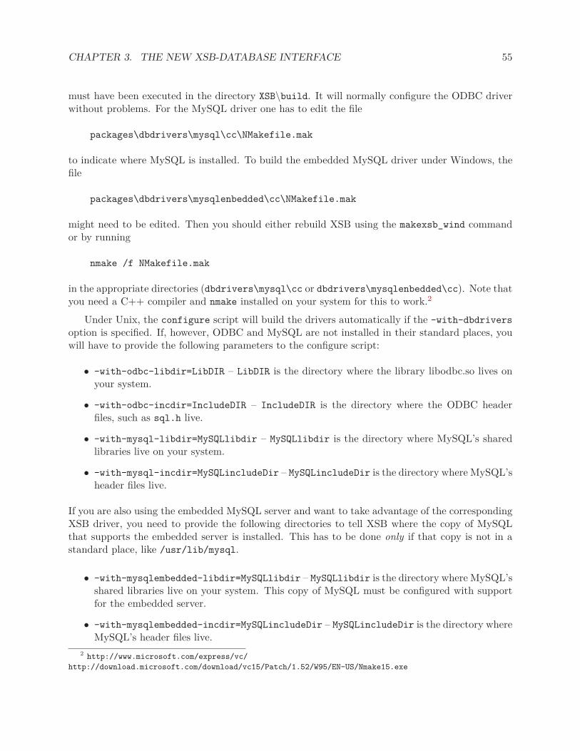
CHAPTER 3. THE NEW XSB-DATABASE INTERFACE 55
must have been executed in the directory XSB\build. It will normally configure the ODBC driverwithout problems. For the MySQL driver one has to edit the file
packages\dbdrivers\mysql\cc\NMakefile.mak
to indicate where MySQL is installed. To build the embedded MySQL driver under Windows, thefile
packages\dbdrivers\mysqlenbedded\cc\NMakefile.mak
might need to be edited. Then you should either rebuild XSB using the makexsb_wind commandor by running
nmake /f NMakefile.mak
in the appropriate directories (dbdrivers\mysql\cc or dbdrivers\mysqlenbedded\cc). Note thatyou need a C++ compiler and nmake installed on your system for this to work.2
Under Unix, the configure script will build the drivers automatically if the –with-dbdrivers
option is specified. If, however, ODBC and MySQL are not installed in their standard places, youwill have to provide the following parameters to the configure script:
• –with-odbc-libdir=LibDIR – LibDIR is the directory where the library libodbc.so lives onyour system.
• –with-odbc-incdir=IncludeDIR – IncludeDIR is the directory where the ODBC headerfiles, such as sql.h live.
• –with-mysql-libdir=MySQLlibdir – MySQLlibdir is the directory where MySQL’s sharedlibraries live on your system.
• –with-mysql-incdir=MySQLincludeDir – MySQLincludeDir is the directory where MySQL’sheader files live.
If you are also using the embedded MySQL server and want to take advantage of the correspondingXSB driver, you need to provide the following directories to tell XSB where the copy of MySQLthat supports the embedded server is installed. This has to be done only if that copy is not in astandard place, like /usr/lib/mysql.
• –with-mysqlembedded-libdir=MySQLlibdir – MySQLlibdir is the directory where MySQL’sshared libraries live on your system. This copy of MySQL must be configured with supportfor the embedded server.
• –with-mysqlembedded-incdir=MySQLincludeDir – MySQLincludeDir is the directory whereMySQL’s header files live.
2 http://www.microsoft.com/express/vc/
http://download.microsoft.com/download/vc15/Patch/1.52/W95/EN-US/Nmake15.exe

CHAPTER 3. THE NEW XSB-DATABASE INTERFACE 56
Under Cygwin, the ODBC libraries come with the distribution; they are located in the directory/cygdrive/c/cygwin/lib/w32api/ and are called odbc32.a and odbccp32.a. (Check if yourinstallation is complete and has these libraries!) Otherwise, the configuration of the interfaceunder Cygwin is same as in unix (you do not need to provide any ODBC-specific parameters tothe configure script under Cygwin).
If at the time of configuring XSB some database packages (e.g., MySQL) are not installed onyour system, you can install them later and configure the XSB interface to them then. For instance,to configure the ODBC interface separately, you can type
cd packages/dbdrivers/odbc
configure
Again, if ODBC is installed in a non-standard location, you might need to supply the options–with-odbc-libdir and –with-odbc-incdir to the configure script. Under Cygwin ODBC isalways installed in a standard place, and configure needs no additional parameters.
Under Windows, separate configuration of the XSB-DB interfaces is also possible, but you needVisual Studio installed. For instance, to configure the MySQL interface, type
cd packages\dbdrivers\mysql\cc
nmake /f NMakefile.mak
As before, you might need to edit the NMakefile.mak script to tell the compiler where the requiredMySQL’s libraries are. You also need the file packages\dbdrivers\mysql\mysql_init.P with thefollowing content:
:- export mysql_info/2.
mysql_info(support, ’yes’).
mysql_info(libdir, ’’).
mysql_info(ccflags, ’’).
mysql_info(ldflags, ’’).
Similarly, to configure the ODBC interface, do
cd packages\dbdrivers\odbc\cc
nmake /f NMakefile.mak
You will also need to create the file packages\dbdrivers\odbc\odbc_init.P with the followingcontents:
:- export odbc_info/2.
odbc_info(support, ’yes’).
odbc_info(libdir, ’’).
odbc_info(ccflags, ’’).
odbc_info(ldflags, ’’).

CHAPTER 3. THE NEW XSB-DATABASE INTERFACE 57
3.3 Using the Interface
We use the student database as our example to illustrate the usage of the XSB-DB interface inthis manual. The schema of the student database contains three columns viz. the student name,the student id, and the name of the advisor of the student.
The XSB-DB package has to be first loaded before using any of the predicates. This is done bythe call:
| ?- [dbdrivers].
Next, the driver to be used for connecting to the database has to be loaded. Currently, theinterface has support for a native MySQL driver (using the MySQL C API), and an ODBC driver.For example, to load the ODBC driver call:
| ?- load_driver(odbc).
Similarly, to load the mysql driver call:
| ?- load_driver(mysql).
or
| ?- load_driver(mysqlembedded).
3.3.1 Connecting to and Disconnecting from Databases
There are two predicates for connecting to databases, db_connect/5 and db_connect/6. Thedb_connect/5 predicate is for ODBC connections, while db_connect/6 is for other (non-ODBC)database drivers.
| ?- db_connect(+Handle, +Driver, +DSN, +User, +Password).
| ?- db_connect(+Handle, +Driver, +Server, +Database, +User, +Password).
The db_connect/5 predicate assumes that an entry for a data source name (DSN) exists in theodbc.ini file. The Handle is the connection handle name used for the connection. The Driver isthe driver being used for the connection. The User and Password are the user name and passwordbeing used for the connection. The user is responsible for giving the name to the handle. Toconnect to the data source mydb using the user name xsb and password xsb with the odbc driver,the call is as follows:
| ?- db_connect(ha, odbc, mydb, xsb, xsb).

CHAPTER 3. THE NEW XSB-DATABASE INTERFACE 58
where ha is the user-chosen handle name (a Prolog atom) for the connection.
The db_connect/6 predicate is used for drivers other than ODBC. The arguments Handle,Driver, User, and Password are the same as for db_connect/5. The Server and Database
arguments specify the server and database to connect to. For example, for a connection to adatabase called test located on the server wolfe with the user name xsb, the password foo, andusing the mysql driver, the call is:
| ?- db_connect(ha, mysql, wolfe, test, xsb, foo).
where ha is the handle name the user chose for the connection.
If the connection is successfully made, the predicate invocation will succeed. This step isnecessary before anything can be done with the data sources since it gives XSB the opportunity toinitialize system resources for the session.
To close a database connection use:
| ?- db_disconnect(Handle).
where handle is the connection handle name. For example, to close the connection to above mysqldatabase call:
| ?- db_disconnect(ha).
and XSB will give all the resources it allocated for this session back to the system.
3.3.2 Querying Databases
The interface supports two types of querying. In direct querying, the query statement is notprepared while in prepared querying the query statement is prepared before being executed. Theresults from both types of querying are retrieved tuple at a time. Direct querying is done by thepredicate:
| ?- db_query(ConnectionHandle, QueryHandle, SQLQueryList, ReturnList).
ConnectionHandle is the name of the handle used for the database connection. QueryHandle isthe name of the query handle for this particular query. For prepared queries, the query handle isused both in order to execute the query and to close it and free up space. For direct querying, thequery handle is used only for closing query statements (see below). The SQLQueryList is a list ofterms which is used to build the SQL query. The terms in this list are ground atoms. ReturnListis a list of variables each of which correspond to a return value in the query. It is upto the user tospecify the correct number of return variables corresponding to the query. Also, as in the case of aconnection handle, the user is responsible for giving the name to the query handle. For example, aquery on the student database to select all the students for a given advisor is accomplished by thecall:
CHAPTER 3. THE NEW XSB-DATABASE INTERFACE 59
| ?- X = adv,
db_query(ha, qa, [’select T.name from student T where T.advisor = ’, X], [P]),
fail.
where ha and qa are respectively the connection handle and query handle name the user chose.
Observe that the query list is composed of the SQL string and a ground value for the advisor.The return list is made of one variable corresponding to the student name. The failure drive loopretrieves all the tuples.
Preparing a query is done by the call to the predicate:
| ?- db_prepare(ConnectionHandle, QueryHandle, SQLQueryList).
As before, ConnectionHandle and QueryHandle specify the handles for the connection and thequery. The SQLQueryList is a list of terms which build up the query string. The placeholder ‘?’is used for values which have to be bound during the execution of the statement. For example, toprepare a query for selecting the advisor name for a student name using our student database:
| ?- db_prepare(ha, qa, [’select T.advisor from student T where T.name = ?’]).
A prepared statement is executed using the predicate:
| ?- db_prepare_execute(QueryHandle, BindList, ReturnList).
The BindList contains the ground values corresponding to the ‘?’ in the prepared statement.The ReturnList is a list of variables for each argument in a tuple of the result set.
For direct querying, the query handle is closed automatically when all the tuples in the resultset have been retrieved. In order to explicitly close a query handle, and free all the resourcesassociated with the handle, a call is made to the predicate:
| ?- db_statement_close(QueryHandle).
where QueryHandle is the query handle for the statement to be closed.
The interface is also able to transparently handle Prolog terms. Users can both save and retrieveterms without any special processing.
3.4 Error Handling
Each predicate in the XSB-DB interface throws an exception with the functor
xsb_error(database(Number), Message)

CHAPTER 3. THE NEW XSB-DATABASE INTERFACE 60
where Number is a string with the error number and Message is a string with a slightly detailederror message. It is upto the user to catch this exception and proceed with error handling. Thisis done by the throw-catch error handling mechanism in XSB. For example, in order to catch theerror which will be thrown when the user attempts to close a database connection for a handle (ha)which does not exist:
| ?- catch(db_disconnect(ha),
xsb_error(database(Number), Message), handler(Number, Message)).
It is the user’s responsibility to define the handler predicate which can be as simple as printingout the error number and message or may involve more complicated processing.
A list of error numbers and messages that are thrown by the XSB-DB interface is given below:
• XSB_DBI_001: XSB_DBI ERROR: Driver already registeredThis error is thrown when the user tries to load a driver, using the load_driver predicate,which has already been loaded previously.
• XSB_DBI_002: XSB_DBI ERROR: Driver does not existThis error is thrown when the user tries to connect to a database, using db_connect, with adriver which has not been loaded.
• XSB_DBI_003: XSB_DBI ERROR: Function does not exist in this driverThis error is thrown when the user tries to use a function support for which does not existin the corresponding driver. For example, this error is generated if the user tries to usedb_prepare for a connection established with the mysql driver.
• XSB_DBI_004: XSB_DBI ERROR: No such connection handleThis error is thrown when the user tries to use a connection handle which has not beencreated.
• XSB_DBI_005: XSB_DBI ERROR: No such query handleThis error is thrown when the user tries to use a query handle which has not been created.
• XSB_DBI_006: XSB_DBI ERROR: Connection handle already existsThis error is thrown when the user tries to create a connection handle in db_connect usinga name which already exists as a connection handle.
• XSB_DBI_007: XSB_DBI ERROR: Query handle already existsThis error is thrown when the user tries to create a query handle, in db_query or db_prepare,using a name which already exists as a query handle for a different query.
• XSB_DBI_008: XSB_DBI ERROR: Not all parameters suppliedThis error is thrown when the user tries to execute a prepared statement, using db_prepare_execute,without supplying values for all the parameters in the statement.
• XSB_DBI_009: XSB_DBI ERROR: Unbound variable in parameter listThis error is thrown when the user tries to execute a prepared statement, using db_prepare_execute,without binding all the parameters of the statement.

CHAPTER 3. THE NEW XSB-DATABASE INTERFACE 61
• XSB_DBI_010: XSB_DBI ERROR: Same query handle used for different queriesThis error is thrown when the user issues a prepare statement (db_prepare) using a queryhandle that has been in use by another prepared statement and which has not been closed.Query handles must be closed before reuse.
• XSB_DBI_011: XSB_DBI ERROR: Number of requested columns exceeds thenumber of columns in the queryThis error is thrown when the user db_query specifies more items to be returned in the lastargument than the number of items in the SELECT statement in the corresponding query.
• XSB_DBI_012: XSB_DBI ERROR: Number of requested columns is less thanthe number of columns in the queryThis error is thrown when the user db_query specifies fewer items to be returned in the lastargument than the number of items in the SELECT statement in the corresponding query.
• XSB_DBI_013: XSB_DBI ERROR: Invalid return list in querySomething else is wrong with the return list of the query.
• XSB_DBI_014: XSB_DBI ERROR: Too many open connectionsThere is a limit (200) on the number of open connections.
• XSB_DBI_015: XSB_DBI ERROR: Too many registered driversThere is a limit (100) on the number of database drivers that can be registered at the sametime.
• XSB_DBI_016: XSB_DBI ERROR: Too many active queriesThere is a limit (2000) on the number of queries that can remain open at any given time.
3.5 Notes on specific drivers
ODBC Driver
The ODBC driver has been tested in Linux using the unixodbc driver manager. It currentlysupports the following functionality: (a) connecting to a database using a DSN, (b) direct queryingof the database, (c) using prepared statements to query the database, (d) closing a statementhandle, and (d) disconnecting from the database. The ODBC driver has also been tested underWindows and Cygwin.
MySQL Driver
The MySQL driver provides access to the native MySQL C API. Currently, it has support for thefollowing functionality: (a) connecting to a database using db_connect, (b) direct querying of thedatabase, (c) using prepared statements to query the database, (d) closing a statement handle, and(e) disconnecting from the database.
The MySQL driver has been tested under Linux and Windows.

CHAPTER 3. THE NEW XSB-DATABASE INTERFACE 62
Driver for the Embedded MySQL Server
This driver provides access to the Embedded MySQL Server Library libmysqld. Currently, it hassupport for the following functionality: (a) connecting to a database db_connect, (b) direct query-ing of the database, (c) using prepared statements to query the database, (d) closing a statementhandle, and (e) disconnecting from the database.
The MySQL driver for Embedded MySQL Server has been tested under Linux.
In order to use this driver, you will need:
• MySQL with Embedded Server installed on your machine. If your don’t have a precompiledbinary distribution of MySQL, which was configured with libmysqld support (the embed-ded server library), you will need to build MySQL from sources and configure it with the–with-embedded-server option.
• append to /etc/my.cnf (or /etc/mysql/my.cnf – whichever is used on your machine) or∼/.my.cnf:
[mysqlembedded_driver_SERVER]
language = /usr/share/mysql/english
datadir = .....
You will probably need to replace /usr/share/mysql/english with a directory appropriatefor your MySQL installation.
You might also need to set the datadir option to specify the directory where the databasesmanaged by the embedded server are to be kept. This has to be done if there is a possibilityof running the embedded MySQL server alongside the regular MySQL server. In that case,the datadir directory of the embedded server must be different from the datadir directory ofthe regular server (which is likely to be specified using the datadir option in /etc/my.cnf or/etc/mysql/my.cnf. This is because specifying the same directory might lead to a corruptionof your databases. See http://dev.mysql.com/doc/refman/5.1/en/multiple-servers.html
for further details on running multiple servers.
Please note that loading the embedded MySQL driver increases the memory footprint of XSB.This additional memory is released automatically when XSB exits. If you need to release thememory before exiting XSB, you can call driverMySQLEmbedded_lib_end after disconnectingfrom MySQL. Note that once driverMySQLEmbedded_lib_end is called, no further connectionsto MySQL are allowed from the currently running session of XSB (or else XSB will exit abnor-mally).

Chapter 4
Introduction to XSB Packages
An XSB package is a piece of software that extends XSB functionality but is not critical to pro-gramming in XSB. Around a dozen packages are distributed with XSB, ranging from simple meta-interpreters to complex software systems. Some packages provide interfaces from XSB to othersoftware systems, such as Perl, SModels or Web interfaces (as in the libwww package). Others,such as the CHR and Flora packages, extend XSB to different programming paradigms.
Each package is distributed in the $XSB_DIR/packages subdirectory, and has two parts: aninitialization file, and a subdirectory in which package source code files and executables are kept.For example, the xsbdoc package has files xsbdoc.P, xsbdoc.xwam, and a subdirectory, xsbdoc.If a user doesn’t want to retain xsbdoc (or any other package) he or she may simply remove theinitialization files and the associated subdirectory without affecting the core parts of the XSBsystem.
Several of the packages are documented in this manual in the various chapters that follow.However, many of the packages contain their own manuals. For these packages, we provide only asummary of their functionality in Chapter 14.
63

Chapter 5
Wildcard Matching
By Michael Kifer
XSB has an efficient interface to POSIX wildcard matching functions. To take advantage of thisfeature, you must build XSB using a C compiler that supports POSIX 2.0 (for wildcard matching).This includes GCC and probably most other compilers. This also works under Windows, providedyou install Cygnus’ CygWin and use GCC to compile 1.
The wildmatch package provides the following functionality:
1. Telling whether a wildcard, like the ones used in Unix shells, match against a given string.Wildcards supported are of the kind available in tcsh or bash. Alternating characters (e.g.,“[abc]” or “[^abc]”) are supported.
2. Finding the list of all file names in a given directory that match a given wildcard. This facilitygeneralizes directory/2 (in module directory), and it is much more efficient.
3. String conversion to lower and upper case.
To use this package, you need to type:
| ?- [wildmatch].
If you are planning to use it in an XSB program, you need this directive:
:- import glob_directory/4, wildmatch/3, convert_string/3 from wildmatch.
The calling sequence for glob_directory/4 is:
glob_directory(+Wildcard, +Directory, ?MarkDirs, -FileList)
1This package has not yet been ported to the multi-threaded engine.
64
CHAPTER 5. WILDCARD MATCHING 65
The parameter Wildcard can be either a Prolog atom or a Prolog string. Directory is also anatom or a string; it specifies the directory to be globbed. MarkDirs indicates whether directorynames should be decorated with a trailing slash: if MarkDirs is bound, then directories will be sodecorated. If MarkDirs is an unbound variable, then trailing slashes will not be added.
FileList gets the list of files in Directory that match Wildcard. If Directory is bound to anatom, then FileList gets bound to a list of atoms; if Directory is a Prolog string, then FileList
will be bound to a list of strings as well.
This predicate succeeds is at least one match is found. If no matches are found or if Directory
does not exist or cannot be read, then the predicate fails.
The calling sequence for wildmatch/3 is as follows:
wildmatch(+Wildcard, +String, ?IgnoreCase)
Wildcard is the same as before. String represents the string to be matched against Wildcard.Like Wildcard, String can be an atom or a string. IgnoreCase indicates whether case of lettersshould be ignored during matching. Namely, if this argument is bound to a non-variable, thenthe case of letters is ignored. Otherwise, if IgnoreCase is a variable, then the case of letters ispreserved.
This predicate succeeds when Wildcard matches String and fails otherwise.
The calling sequence for convert_string/3 is as follows:
convert_string(+InputString, +OutputString, +ConversionFlag)
The input string must be an atom or a character list. The output string must be unbound. Itstype will “atom” if so was the input and it will be a character list if so was the input string. Theconversion flag must be the atom tolower or toupper.
This predicate always succeeds, unless there was an error, such as wrong type argument passedas a parameter.

Chapter 6
pcre: Pattern Matching andSubstitution Using PCRE
By Mandar Pathak
6.1 Introduction
This package employs the PCRE library to enable XSB perform pattern matching and stringsubstitution based on Perl regular expressions.
6.2 Pattern matching
The pcre package provides two ways of doing pattern matching: first-match mode and bulk-matchmode. The syntax of the pcre:match/4 predicate is:
?- pcre:match(+Pattern, +Subject, -MatchList, +Mode).
To find only the first match, the Mode parameter must be set to the atom one. To find allmatches, the Mode parameter is set to the atom bulk. The result of the matching is returned as alist of the form:
match(Match,Prematch,Postmatch,[Subpattern1, Subpattern2,. . . ])
The Pattern and the Subject arguments of pcre:match must be XSB atoms. If there is amatch in the subject, then the result is returned as a list of the form shown above. Match refersto the substring which matched the entire pattern. Prematch contains part of the subject-stringthat precedes the matched substring. Postmatch contains part of the subject following the matchedsubstring. The list of subpatterns (the 4-th argument of the match data structure) corresponds tothe substrings which matched the parenthesized expressions in the given pattern. For example:
66
CHAPTER 6. PCRE: PATTERN MATCHING AND SUBSTITUTION USING PCRE 67
?- pcre:match(’(\d{5}-\d{4})\ [A-Z]{2}’,
’Hello12345-6789 NYwalk’, X, ’one’).
X = [match(12345-6789 NY,Hello,walk,[12345-6789])]
In this example, the match was found for substring ‘12345-6789 NY’. The prematch is ‘Hello’and the postmatch is ‘walk’. The substring ‘12345-6789’ matched the parenthesized expression(\d{5}−\d{4}) and hence it is returned as part of the subpatterns list. Consider another example:
?- pcre:match(’[a-z]+@[a-z]+\.(com|net|edu)’,
’[email protected]@[email protected]’, X, ’bulk’).
X = [match([email protected],,@[email protected],[com]),
match([email protected],a@b.,@d.edu,[net]),
match([email protected],[email protected],@d.edu,[net]),
match([email protected],[email protected],@d.edu,[net]),
match([email protected],[email protected]@c.,,[edu]),
match([email protected],[email protected]@c.n,,[edu]),
match([email protected],[email protected]@c.ne,,[edu])]
This example uses the bulk match mode of the pcre_match/4 to find all possible matcheswhich resemble a very basic email address. In case there is no prematch or postmatch to a matchedsubstring, an empty string is returned.
In general, there can be any number of parenthesized subtatterns in a given pattern and thesubpattern match-list in the 4-th argument of the match data structure can have 0, 1, 2, or moreelements.
6.3 String Substitution
The pcre package also provides a way to perform string substitution via the pcre:substitute/4
predicate. It has the following syntax:
?- pcre:substitute(+Pattern, +Subject, +Substitution, -Result).
Pattern is the regular expression against which Subject is matched. Each match found is thenreplaced by the Substitution, and the result is returned in the variable Result. Here, Pattern,Subject and Substitution have to be XSB atoms whereas Result must be an unbound variable. Thefollowing example illustrates the use of this predicate:
?- pcre:substitute(’is’,’This is a Mississippi issue’, ’was’, X).
X = Thwas was a Mwasswassippi wassue
Note that the predicate pcre:substitute/4 always works in a bulk mode. If one needs tosubstitute only one occurrence of a pattern, this is easy to do using the pcre:match/4 predicate.For instance, if one wants to replace the third occurrence of “is” in the above string, we couldissue the query

CHAPTER 6. PCRE: PATTERN MATCHING AND SUBSTITUTION USING PCRE 68
?- pcre:match(’is’,’This is a Mississippi issue’,X,bulk).
take the third element in the returned list, which is
match(is,’This is a M’,’sissippi issue’,[])
and then concatenate the 2-nd argument with “was” and with the 3-d argument of that match datastructure.
More examples of the use of the pcre package can be found in
$XSBDIR/examples/pcretest.P
6.4 Installation and configuration
XSB’s pcre package requires that the PCRE library is installed. For Windows, the PCRE library filesare included with the installation. For Linux and Mac, the libpcre and libpcre-dev packagesmust be installed using the distribution’s package manager.
6.4.1 Configuring for Linux, Mac, and other Unices
If a particular Linux distribution does not include these libraries they must be downloaded andbuilt manually. Please visit
http://www.pcre.org/
to download the latest distribution and follow the instructions given with the package.
To configure pcre on Linux, Mac, or on some other Unix variant, switch to the XSB/build
directory and type:
cd ../packages/pcre
./configure
./makexsb
6.4.2 Configuring for Windows
Configuring pcre on Windows requires creating the DLL for Windows. To create the DLL, openthe Visual C++ command prompt, switch to the root XSB directory, and type:
cd packages\pcre\cc
nmake /f NMakefile.mak

CHAPTER 6. PCRE: PATTERN MATCHING AND SUBSTITUTION USING PCRE 69
This builds the DLL required by XSB’s pcre package on Windows. To ensure that the buildwent ahead smoothly, open the directory
{XSB_DIR}\config\x86-pc-windows\bin
and verify that the file pcre4pl.dll exists there.
Once the package has been configured, it must be loaded before it can be used:
?- [pcre].

Chapter 7
curl: The XSB Internet AccessPackage
By Aneesh Ali
7.1 Introduction
The curl package is an interface to the libcurl library, which provides access to most of thestandard Web protocols. The supported protocols include FTP, FTPS, HTTP, HTTPS, SCP,SFTP, TFTP, TELNET, DICT, LDAP, LDAPS, FILE, IMAP, SMTP, POP3 and RTSP. Libcurlsupports SSL certificates, HTTP POST, HTTP PUT, FTP uploading, HTTP form based upload,proxies, cookies, user+password authentication (Basic, Digest, NTLM, Negotiate, Kerberos4), filetransfer resume, http proxy tunneling etc.
The curl package accepts input in the form of URLs and Prolog atoms. To load the curl
package, the user should type
?- [curl].
The curl package is integrated with file I/O of XSB in a transparent fashion and for many purposesWeb pages can be treated just as yet another kind of a file. We first explain how Web pages canbe accessed using the standard file I/O feature and then describe other predicates, which providea lower-level interface.
7.2 Integration with File I/O
The curl package is integrated with XSB File I/O so that a web page can be opened as any otherfile.Once a Web page is opened, it can be read or written just like the a normal file.
70

CHAPTER 7. CURL: THE XSB INTERNET ACCESS PACKAGE 71
7.2.1 Opening a Web Document
Web documents are opened by the usual predicates see/1, open/3, open/4.
see(url(+Url))
see(url(+Url,Options))
open(url(+Url), +Mode, -Stream)
open(url(+Url), +Mode, -Stream, +Options)
Url is an atom that specifies a URL. Stream is the file stream of the open file. Mode can be
read to create an input stream or write, to create an output stream. For reading, thecontents of the Web page are cached in a temporary file. For writing, a temporary empty fileis created. This file is posted to the corresponding URL at closing.
The Options parameter is a list that controls loading. Members of that list can be of thefollowing form:
redirect(Bool)Specifies the redirection option. The supported values are true and false. If true, anynumber of redirects is allowed. If false, redirections are ignored. The default is true.
secure(CrtName)Specifies the secure connections (https) option. CrtName is the name of the file holdingone or more certificates to verify the peer with.
auth(UserName, Password)Sets the username and password basic authentication.
timeout(Seconds)Sets the maximum time in seconds that is allowed for the transfer operation.
user_agent(Agent)Sets the User-Agent: header in the http request sent to the remote server.
7.2.2 Closing a Web Document
Web documents opened by the predicates see/1, open/3, and open/4 above must be closed bythe predicates close/2 or close/3. The data written to the stream is first posted to the URL. Ifthat succeeds, the stream is closed. ???? And if it does not suceed????
close(+Stream, +Source)
close(+Stream, +Source, +Options)Source can be of the form url(url). Stream is a file stream. Options is a list of optionssupported normally for close.

CHAPTER 7. CURL: THE XSB INTERNET ACCESS PACKAGE 72
7.3 Low Level Predicates
This section describes additional predicates provided by the curl packages, which extend thefunctionality provided by the file I/O integration.
7.3.1 Loading web documents
Web documents are loaded by the predicate load_page/5, which has many options. The param-eters of this predicate are described below.
load_page(+Source, +Options, -Properties, -Content, -Warn)Source can be of the form url(url) or an atom url (check!!!). The document is returned inContent. Warn is bound to a (possibly empty) list of warnings generated during the process.
Properties is bound to a list of properties of the document. They include Directory name,File name, File suffix, Page size, and Page time. The load_page/5 predicate caches a copyof the Web page that it fetched from the Web in a local file, which is specified by the aboveproperties Directory name, File name, and File suffix. The remaining two parameters indicatethe size and the last modification time of the fetched Web page. The directory and the filename The Options parameter is the same as in the URL opening predicates.
7.3.2 Retrieve the properties of a web document
The properties of a web document are loaded by the predicates url_properties/3 and url_properties/2.
url_properties(+Url, +Options, -Properties)The Options and Properties are same as in load_page/5.
url_properties(+Url, -Properties)What are the default options???
7.3.3 Encode Url
Sometimes it is necessary to convert a URL string into something that can be used, for example,as a file name. This is done by the following predicate.
url_properties(+Source, -Properties)(???? url_properties for encoding??? Explain the difference with url_properties)
Source has the form url(url) or an atom url, where url is an atom. (check!!!) Properties isbound to a list of properties of the URL. They include Directory Name, File Name and, FileSuffix of the URL.
CHAPTER 7. CURL: THE XSB INTERNET ACCESS PACKAGE 73
7.3.4 Obtaining the Redirection URL
If the originally specified URL was redirected, the URL of the page that was actually fetched byload_page/5 can be found with the help of the following predicate:
get_redir_url(+Source, -UrlNew)Source can be of the form url(url), file(filename) or a string.
7.4 Installation and configuration
The curl package of XSB requires that the libcurl package is installed. For Windows, the libcurl
library files are included with the installation. For Linux and Mac, the libcurl and libcurl-dev
packages need to be installed using the distribution’s package manager. In some Linux distributions,libcurl-dev might be called libcurl-gnutls-dev or libcurl-openssl-dev. In addition, therelease number might be attached. For instance, libcurl4 and libcurl4-openssl-dev.
If a particular Linux distribution does not include the above packages and for other Unixvariants, the libcurl package must be downloaded and built manually. See
http://curl.haxx.se/download.html
To configure curl on Linux, Mac, or on some other Unix variant, switch to the XSB/build directoryand type
cd XSB/packages/curl
./configure
./makexsb
5

Chapter 8
sgml and xpath: SGML/XML/HTMLParsers and XPath
By Rohan Shirwaikar
8.1 Introduction
This suite of packages consists of the sgml package, which can parse XML, HTML, XHTML, andeven SGML documents and the xpath package, which supports XPath queries on XML documents.The sgml package is an adaptation of a similar package in SWI Prolog and a port of SWI’s codebasewith some minor changes. The xpath package provides an interface to the popular libxml2 library,which supports XPath and XML parsing, and is used in Mozilla based browsers. At present, theXML parsing capabilities of libxml2 are not utilized explicitly in XSB, but such support might beprovided in the future. The sgml package does not rely on libxml2 1.
Installation and configuration. The sgml package does not require any installation steps underUnix-based systems or under Cygwin. Under native Windows, if you downloaded XSB from CVS,you need to compile the package as follows:
cd XSB\packages\sgml\cc
nmake /f NMakefile.mak
You need MS Visual Studio for that. If you downloaded a prebuilt version of XSB, then the sgml
package should have already been compiled for you and no installation is required.
The details of the xpath package and the corresponding configuration instructions appear inSection 8.4.
1This package has not yet been tested for thread-safety
74

CHAPTER 8. SGML AND XPATH: SGML/XML/HTML PARSERS AND XPATH 75
8.2 Overview of the SGML Parser
The sgml package accepts input in the form of files, URLs and Prolog atoms. To load the sgml
parser, the user should type
?- [sgml].
at the prompt. If test.html is a file with the following contents
<!DOCTYPE HTML PUBLIC "-//W3C//DTD HTML 3.2//EN">
<html>
<head>
<title>Demo</title>
</head>
<body>
<h1 align=center>This is a demo</h1>
<p>Paragraphs in HTML need not be closed.
<p>This is called ‘omitted-tag’ handling.
</body>
</html>
then the following call
?- load_html_structure(file(’test.html’), Term, Warn).
will parse the document and bind Term to the following Prolog term:
[ element(html,
[],
[ element(head,
[],
[ element(title,
[],
[ ’Demo’
])
]),
element(body,
[],
[ ’\n’,
element(h1,
[ align = center

CHAPTER 8. SGML AND XPATH: SGML/XML/HTML PARSERS AND XPATH 76
],
[ ’This is a demo’
]),
’\n\n’,
element(p,
[],
[ ’Paragraphs in HTML need not be closed.\n’
]),
element(p,
[],
[ ’This is called ‘omitted-tag\’ handling.’
])
])
])
].
The XML document is converted into a list of Prolog terms of the form element(Name,Attributes,Content ).Each term corresponds to an XML element. Name represents the name of the element. Attributesis a list of attribute-value pairs of the element. Content is a list of child-elements and CDATA. Forinstance,
<aaa>fooo<bbb>foo1</bbb></aaa>
will be parsed as
element(aaa,[],[fooo, element(bbb,[],[foo1])])
Entities (e.g. <) are returned as part of CDATA, unless they cannot be represented. Seeload_sgml_structure/3 for details.
8.3 Predicate Reference
8.3.1 Loading Structured Documents
SGML, HTML, and XML documents are parsed by the predicate load_structure/4, which hasmany options. For convenience, a number of commonly used shorthands are provided to parseSGML, XML, HTML, and XHTML documents respectively.
load_sgml_structure(+Source, -Content, -Warn)
load_xml_structure(+Source, -Content, -Warn)
load_html_structure(+Source, -Content, -Warn)
load_xhtml_structure(+Source, -Content, -Warn)

CHAPTER 8. SGML AND XPATH: SGML/XML/HTML PARSERS AND XPATH 77
The parameters of these predicates have the same meaning as those in load_structure/4, andare described below.
The above predicates (in fact, just load_xml_structure/3 and load_html_structure/3) arethe most commonly used predicates of the sgml package. The other predicates described in thissection are needed only for advanced uses of the package.
load_structure(+Source, -Content, +Options, -Warn)Source can have one of the following forms: url(url), file(file name), string(’document asa Prolog atom’). The parsed document is returned in Content. Warn is bound to a (possiblyempty) list of warnings generated during the parsing process. Options is a list of parametersthat control parsing, which are described later.
The list Content can have the following members:
A Prolog atomAtoms are used to represent character strings, i.e., CDATA.
element(Name, Attributes, Content)Name is the name of the element tag. Since SGML is case-insensitive, all element namesare returned as lowercase atoms.
Attributes is a list of pairs the form Name=Value, where Name is the name of an at-tribute and Value is its value. Values of type CDATA are represented as atoms. Thevalues of multi-valued attributes (NAMES, etc.) are represented as a lists of atoms.Handling of the attributes of types NUMBER and NUMBERS depends on the setting ofthe number(+NumberMode) option of set_sgml_parser/2 or load_structure/3 (seelater). By default the values of such attributes are represented as atoms, but thenumber(...) option can also specify that these values must be converted to Prologintegers.
Content is a list that represents the content for the element.
entity(Code)If a character entity (e.g., Α) is encountered that cannot be represented in theProlog character set, this term is returned. It represents the code of the encounteredcharacter (e.g., entity(913)).
entity(Name)This is a special case of entity(Code), intended to handle special symbols by theirname rather than character code. If an entity refers to a character entity holding a singlecharacter, but this character cannot be represented in the Prolog character set, this termis returned. For example, if the contents of an element is Α < Β then itwill be represented as follows:
[ entity(’Alpha’), ’ < ’, entity(’Beta’) ]
Note that entity names are case sensitive in both SGML and XML.
sdata(Text)If an entity with declared content-type SDATA is encountered, this term is used. Thedata of the entity instantiates Text.

CHAPTER 8. SGML AND XPATH: SGML/XML/HTML PARSERS AND XPATH 78
ndata(Text)If an entity with declared content-type NDATA is encountered, this term is used. Thedata instantiates Text.
pi(Text)If a processing instruction is encountered (<?...?>), Text holds the text of the processinginstruction. Please note that the <?xml ...?> instruction is ignored and is not treatedas a processing instruction.
The Options parameter is a list that controls parsing. Members of that list can be of thefollowing form:
dtd(?DTD)Reference to a DTD object. If specified, the <!DOCTYPE ...> declaration supplied withthe document is ignored and the document is parsed and validated against the providedDTD. If the DTD argument is a variable, then a the variable DTD gets bound to theDTD object created out of the DTD supplied with the document.
dialect(+Dialect)Specify the parsing dialect. The supported dialects are sgml (default), xml and xmlns.
space(+SpaceMode)Sets the space handling mode for the initial environment. This mode is inherited bythe other environments, which can override the inherited value using the XML reservedattribute xml:space. See Section 8.3.2 for details.
number(+NumberMode)Determines how attributes of type NUMBER and NUMBERS are handled. If token is specified(the default) they are passed as an atom. If integer is specified the parser attempts toconvert the value to an integer. If conversion is successful, the attribute is representedas a Prolog integer. Otherwise the value is represented as an atom. Note that SGMLdefines a numeric attribute to be a sequence of digits. The - (minus) sign is not allowedand 1 is different from 01. For this reason the default is to handle numeric attributes astokens. If conversion to integer is enabled, negative values are silently accepted and theminus sign is ignored.
defaults(+Bool)Determines how default and fixed attributes from the DTD are used. By default, defaultsare included in the output if they do not appear in the source. If false, only theattributes occurring in the source are emitted.
file(+Name)Sets the name of the input file for error reporting. This is useful if the input is a streamthat is not coming from a file. In this case, errors and warnings will not have the file namein them, and this option allows one to force inclusion of a file name in such messages.
line(+Line)Sets the starting line-number for reporting errors. For instance, if line(10) is specifiedand an error is found at line X then the error message will say that the error occurredat line X+10. This option is used when the input stream does not start with the firstline of a file.

CHAPTER 8. SGML AND XPATH: SGML/XML/HTML PARSERS AND XPATH 79
max_errors(+Max)Sets the maximum number of errors. The default is 50. If this number is reached, thefollowing exception is raised:
error(limit_exceeded(max_errors, Max), _)
8.3.2 Handling of White Spaces
Four modes for handling white-spaces are provided. The initial mode can be switched using thespace(SpaceMode) option to load_structure/3 or set_sgml_parser/2. In XML mode, themode is further controlled by the xml:space attribute, which may be specified both in the DTDand in the document. The defined modes are:
space(sgml)Newlines at the start and end of an element are removed. This is the default mode for theSGML dialect.
space(preserve)White space is passed literally to the application. This mode leaves all white space handlingto the application. This is the default mode for the XML dialect.
space(default)In addition to sgml space-mode, all consecutive whitespace is reduced to a single space-character.
space(remove)In addition to default, all leading and trailing white-space is removed from CDATA objects.If, as a result, the CDATA becomes empty, nothing is passed to the application. This mode isespecially handy for processing data-oriented documents, such as RDF. It is not suitable fornormal text documents. Consider the HTML fragment below. When processed in this mode,the spaces surrounding the three elements in the example below are lost. This mode is notpart of any standard: XML 1.0 allows only default and preserve.
Consider adjacent <b>bold</b> <ul>and</ul> <it>italic</it> words.
The parsed term will be [’Consider adjacent’,element(b,[],[bold]),element(ul,[],
[and]),element(it,[],[italics]),words].
8.3.3 XML documents
The parser can operate in two modes: the sgml mode and the xml mode, as defined by thedialect(Dialect) option. HTML is a special case of the SGML mode with a particular DTD.Regardless of this option, if the first line of the document reads as below, the parser is switchedautomatically to the XML mode.
<?xml ... ?>
CHAPTER 8. SGML AND XPATH: SGML/XML/HTML PARSERS AND XPATH 80
Switching to XML mode implies:
• XML empty elementsThe construct <element attribute ... attribute/> is recognized as an empty element.
• Predefined entitiesThe following entities are predefined: < (<), > (>), & (&), ' (’) and "
(").
• Case sensitivityIn XML mode, names of tags and attributes are case-sensitive, except for the DTD reservednames (i.e. ELEMENT, etc.).
• Character classesIn XML mode, underscore (_) and colon (:) are allowed in names.
• White-space handlingWhite space mode is set to preserve. In addition, the XML reserved attribute xml:spaceis honored; it may appear both in the document and the DTD. The remove extension (seespace(remove) earlier) is allowed as a value of the xml:space attribute. For example, theDTD statement below ensures that the pre element preserves space, regardless of the defaultprocessing mode.
<!ATTLIST pre xml:space nmtoken #fixed preserve>
XML Namespaces
Using the dialect xmlns, the parser will recognize XML namespace prefixes. In this case, the namesof elements are returned as a term of the format
URL:LocalName
If an identifier has no namespace prefix and there is no default namespace, it is returned as asimple atom. If an identifier has a namespace prefix but this prefix is undeclared, the namespaceprefix rather than the related URL is returned.
Attributes declaring namespaces (xmlns:ns=url) are represented in the translation as regularattributes.
8.3.4 DTD-Handling
The DTD (Document Type Definition) are internally represented as objects that can be created,freed, defined, and inspected. Like the parser itself, it is filled by opening it as a Prolog outputstream and sending data to it. This section summarizes the predicates for handling the DTD.

CHAPTER 8. SGML AND XPATH: SGML/XML/HTML PARSERS AND XPATH 81
new_dtd(+DocType, -DTD, -Warn)Creates an empty DTD for the named DocType. The returned DTD-reference is an opaqueterm that can be used in the other predicates of this package. Warn is the list of warningsgenerated.
free_dtd(+DTD, -Warn)Deallocate all resources associated to the DTD. Further use of DTD is invalid. Warn is thelist of warnings generated.
open_dtd(+DTD, +Options, -Warn)This opens and loads a DTD from a specified location (given in the Options parameter (seenext). DTD represents the created DTD object after the source is loaded. Options is a listoptions. Currently the only option supported is source(location), where location can be of oneof these forms:
url(url)file(fileName)
string(’document as a Prolog atom’).
dtd(+DocType, -DTD, -Warn)Certain DTDs are part of the system and have known doctypes. Currently, ’HTML’ and’XHTML’ are the only recognized built-in doctypes. Such a DTD can be used for parsingsimply by specifying the doctype. Thus, the dtd/3 predicate takes the doctype name, findsthe DTD associated with the given doctype, and creates a dtd object for it. Warn is the listof warnings generated.
dtd(+DocType, -DTD, +DtdFile -Warn)
The predicate parses the DTD present at the location DtdFile and creates the correspond-ing DTD object. DtdFile can have one of the following forms: url(url), file(fileName),string(’document as a Prolog atom’).
8.3.5 Low-level Parsing Primitives
The following primitives are used only for more complex types of parsing, which might not becovered by the load_structure/4 predicate.
new_sgml_parser(-Parser, +Options, -Warn)Creates a new parser. Warn is the list of warnings generated. A parser can be used one ormultiple times for parsing documents or parts thereof. It may be bound to a DTD or theDTD may be left implicit. In this case the DTD is created from the document prologue or (ifit is not in the prologue) parsing is performed without a DTD. The Options list can containthe following parameters:
dtd(?DTD)If DTD is bound to a DTD object, this DTD is used for parsing the document and

CHAPTER 8. SGML AND XPATH: SGML/XML/HTML PARSERS AND XPATH 82
the document’s prologue is ignored. If DTD is a variable, the variable gets bound to acreated DTD. This DTD may be created from the document prologue or build implicitlyfrom the document’s content.
free_sgml_parser(+Parser, -Warn)Destroy all resources related to the parser. This does not destroy the DTD if the parser wascreated using the dtd(DTD ) option. Warn is the list of warnings generated during parsing(can be empty).
set_sgml_parser(+Parser, +Option, -Warn)Sets attributes to the parser. Warn is the list of warnings generated. Options is a list thatcan contain the following members:
file(File)Sets the file for reporting errors and warnings. Sets the linenumber to 1.
line(Line)Sets the starting line for error reporting. Useful if the stream is not at the start of the(file) object for generating proper line-numbers. This option has the same meaning asin the load_structure/4 predicate.
charpos(Offset)Sets the starting character location. See also the file(File) option. Used when thestream does not start from the beginning of a document.
dialect(Dialect)Set the markup dialect. Known dialects:
sgml
The default dialect. This implies markup is case-insensitive and standard SGMLabbreviation is allowed (abbreviated attributes and omitted tags).
xml
This dialect is selected automatically if the processing instruction <?xml ...> isencountered.
xmlns
Process file as XML file with namespace support.
qualify_attributes(Boolean)Specifies how to handle unqualified attributes (i.e., without an explicit namespace) inXML namespace (xmlns) dialect. By default, such attributes are not qualified withnamespace prefixes. If true, such attributes are qualified with the namespace of theelement they appear in.
space(SpaceMode)Define the initial handling of white-space in PCDATA. This attribute is described in Sec-tion 8.3.2.
number(NumberMode)If token is specified (the default), attributes of type number are represented as a Prologatom. If integer is specified, such attributes are translated into Prolog integers. If the
CHAPTER 8. SGML AND XPATH: SGML/XML/HTML PARSERS AND XPATH 83
conversion fails (e.g., due to an overflow) a warning is issued and the value is representedas an atom.
doctype(Element)Defines the top-level element of the document. If a <!DOCTYPE ...> declaration has beenparsed, this declaration is used. If there is no DOCTYPE declaration then the parser can beinstructed to use the element given in doctype(_) as the top level element. This featureis useful when parsing part of a document (see the parse option to sgml_parse/3).
sgml_parse(+Parser, +Options, -Warn)Parse an XML file. The parser can operate in two input and two output modes. Output is astructured term as described with load_structure/4.
Warn is the list of warnings generated. A full description of Options is given below.
document(+Term)A variable that will be unified with a list describing the content of the document (seeload_structure/4).
source(+Source)Source can have one of the following forms: url(url), file(fileName), string(’documentas a Prolog atom’). This option must be given.
content_length(+Characters)Stop parsing after the given number of Characters. This option is useful for parsinginput embedded in envelopes, such as HTTP envelopes.
parse(Unit)Defines how much of the input is parsed. This option is used to parse only parts of afile.
file
Default. Parse everything upto the end of the input.
element
The parser stops after reading the first element. Using source(Stream ), this impliesreading is stopped as soon as the element is complete, and another call may be issuedon the same stream to read the next element.
declaration
This may be used to stop the parser after reading the first declaration. This is usefulif we want to parse only the doctype declaration.
max_errors(+MaxErrors)Sets the maximum number of errors. If this number is exceeded, further writes to thestream will yield an I/O error exception. Printing of errors is suppressed after reachingthis value. The default is 100.
syntax_errors(+ErrorMode)Defines how syntax errors are handled.
quietSuppress all messages.
CHAPTER 8. SGML AND XPATH: SGML/XML/HTML PARSERS AND XPATH 84
printDefault. Print messages.
8.3.6 External Entities
While processing an SGML document the document may refer to external data. This occurs inthree places: external parameter entities, normal external entities and the DOCTYPE declaration.The current version of this tool deals rather primitively with external data. External entities canonly be loaded from a file.
Two types of lines are recognized by this package:
DOCTYPE doctype file
PUBLIC "Id " file
The parser loads the entity from the file specified as file. The file can be local or a URL.
8.3.7 Exceptions
Exceptions are generated by the parser in two cases. The first case is when the user specifies wronginput. For example when specifying
load_structure( string(’<m></m>’), Document, [line(xyz)], Warn)
The string xyz is not in the domain of line. Hence in this case a domain error exception will bethrown.
Exceptions are generated when XML being parsed is not well formed. For example if the inputXML contains
’<m></m1>’
exceptions will be thrown.
In both cases the format of the exception is
error( sgml( error term), error message)
warning( sgml( warning term), warning message)
where error term or warning term can be of the form
• pointer to the parser instance,
• line at which error occurred,
CHAPTER 8. SGML AND XPATH: SGML/XML/HTML PARSERS AND XPATH 85
• error code.
• functor(argument), where functor and argument depend on the type of exception raised. Forexample,
resource-error(no-memory) — if memory is unavailable
permission-error(file-name) — no permission to read a file
A system-error(description) –- internal system error
type-error(expected,actual) — data type error
domain-error(functor,offending-value) — the offending value is not in the domainof the functor. For instance, in load_structure( string(’<m></m>’), Document,
[line(xyz)], Warn), xyz is not in the domain of line.
existence-error(resource) — resource does not exist
limit-exceeded(limit,maxval) — value exceeds the limit.
8.3.8 Unsupported features
The current parser is rather limited. While it is able to deal with many serious documents, it omitsseveral less-used features of SGML and XML. Known missing SGML features include
• NOTATION on entitiesThough notation is parsed, notation attributes on external entity declarations are not repre-sented in the output.
• NOTATION attributesSGML notations may have attributes, declared using <!ATTLIST #NOT name attrib>. Thosedata attributes are provided when you declare an external CDATA, NDATA, or SDATA entity.XML does not support external CDATA, NDATA, or SDATA entities, nor any of the otheruses to which data attributes are put in SGML.
• SGML declarationThe ‘SGML declaration’ is fixed, though most of the parameters are handled through indi-rections in the implementation.
• The RANK featureIt is regarded as obsolete.
• The LINK featureIt is regarded as too complicated.
• The CONCUR featureConcurrent markup allows a document to be tagged according to more than one DTD at thesame time. It is not supported.
• The Catalog filesCatalog files are not supported.

CHAPTER 8. SGML AND XPATH: SGML/XML/HTML PARSERS AND XPATH 86
In the XML mode, the parser recognizes SGML constructs that are not allowed in XML. Alsovarious extensions of XML over SGML are not yet realized. In particular, XInclude is not imple-mented.
8.3.9 Summary of Predicates
dtd/2 Find or build a DTD for a document typefree_dtd/1 Free a DTD objectfree_sgml_parser/1 Destroy a parserload_dtd/2 Read DTD information from a fileload_structure/4 Parse XML/SGML/HTML data into Prolog termload_sgml_structure/3 Parse SGML file into Prolog termload_html_structure/3 Parse HTML file into Prolog termload_xml_structure/3 Parse XML file into Prolog termload_xhtml_structure/3 Parse XHTML file into Prolog termnew_dtd/2 Create a DTD objectnew_sgml_parser/2 Create a new parseropen_dtd/3 Open a DTD object as an output streamset_sgml_parser/2 Set parser options (dialect, source, etc.)sgml_parse/2 Parse the inputxml_name/1 Test atom for valid XML namexml_quote_attribute/2 Quote text for use as an attributexml_quote_cdata/2 Quote text for use as PCDATA
8.4 XPath support
XPath is a query language for addressing parts of an XML document. In XSB, this support is pro-vided by the xpath package. To use this package the libxml2 XML parsing library must be installedon the machine. It comes with most Linux distributions, since it is part of the Gnome desktop,or one can download it from http://xmlsoft.org/. It is available for Linux, Solaris, Windows, andMacOS. Note that both the library itself and the .h files of that library must be installed. In someLinux distributions, the .h files might reside in a separate package from the package that containsthe actual library. For instance, the library (libxml2.so) might be in the package called libxml2
(which is usually installed by default), while the .h files might be in the package libxml2-dev
(which is usually not in default installations).
On Unix-based systems (and MacOS), the package might need to be configured at the timeXSB is configured using XSB’s configure script found in the XSB’s build directory. Normally,if libxml2 is installed by a Linux package manager, nothing special is required: the packagewill be configured by default. If the library is in a non-standard place, then the configure op-tion –with-xpath-dir=directory-of-libxml2 must be given. It must specify the directory wherelib/*/libxml2.so (or libxml2.dylib in Mac) and include/libxml2 can be found.
Examples: If libxml2 is in a default location, then XSB can be configured simply like this:

CHAPTER 8. SGML AND XPATH: SGML/XML/HTML PARSERS AND XPATH 87
./configure
Otherwise, use
./configure --with-xpath-dir=/usr/local
if, for example, libxml2.so is in /usr/local/lib/i386-linux-gnu/libxml2.so and the included.h files are in /usr/local/include/libxml2/*.
On Windows and under Cygwin, the libxml2 library is already included in the XSB distributionand does not need to be downloaded. If you are using a prebuilt XSB distribution for Windows,then you do not need to do anything—the package has already been built for you.
For Cygwin, you only need to run the ./configure script without any options. This needs tobe done regardless of whether you downloaded XSB from CVS or a released prebuilt version.
If you downloaded XSB from CVS and want to use it under native Windows (not Cygwin),then you would need to compile the XPath package, and you need Microsoft’s Visual Studio. Tocompile the package one should do the following:
cd packages\xpath\cc
nmake /f NMakefile.mak
The following section assumes that the reader is familiar with the syntax of XPath and itscapabilities. To load the xpath package, type
:-[xpath].
The program needs to include the following directive:
:- import parse_xpath/4 from xpath.
XPath query evaluation is done by using the parse_xpath predicate.
parse_xpath(+Source, +XPathQuery, -Output, +NamespacePrefixList)Source is a term of the format url(url), file(filename) or string(’XML-document-as-a-string’). It specifies that the input XML document is contained in a file, can be fetched froma URL, or is given directly as a Prolog atom.
XPathQuery is a standard XPath query which is to be evaluated on the XML document inSource.
Output gets bound to the output term. It represents the XML element returned after theXPath query is evaluated on the XML document in Source. The output term is of the formstring(’XML-document’). It can then be parsed using the sgml package described earlier.
NamespacePrefixList is a space separated list of pairs of the form prefix = namespace. Thisspecifies the namespace prefixes that are used in the XPath query.
For example if the xpath expression is ’/x:html/x:head/x:meta’ where x is a prefix thatstands for ’http://www.w3.org/1999/xhtml’, then x would have to be defined as follows:

CHAPTER 8. SGML AND XPATH: SGML/XML/HTML PARSERS AND XPATH 88
?- parse_xpath(url(’http://w3.org’), ’/x:html/x:head/x:meta’, O4,
’x=http://www.w3.org/1999/xhtml’).
In the above, the xpath query is ’/x:html/x:head/x:meta’ and the prefix has been definedas ’x=http://www.w3.org/1999/xhtml’.

Chapter 9
rdf: The XSB RDF Parser
By Aneesh Ali
9.1 Introduction
RDF is a W3C standard for representing meta-data about documents on the Web as well asexchanging frame-based data (e.g. ontologies). RDF has a formal data model defined in terms oftriples. In addition, a graph model is defined for visualization and an XML serialization for exchange.This chapter describes the API provided by the XSB RDF parsing package. The package and itsdocumentation are adaptations from SWI Prolog.
9.2 High-level API
The RDF translator is built in Prolog on top of the sgml2pl package, which provides XML parsing.The transformation is realized in two passes. It is designed to operate in various environments andtherefore provides interfaces at various levels. First we describe the top level, which parses RDF-XML file into a list of triples. These triples are not asserted into the Prolog database because it isnot necessarily the final format the user wishes to use and it is not clear how the user might wantto deal with multiple RDF documents. Some options are using global URI’s in one pool, in Prologmodules, or using an additional argument.
load_rdf(+File, -Triples)Same as load_rdf(+File, -Triples, []).
load_rdf(+File, -Triples, +Options)Read the RDF-XML file File and return a list of Triples. Options is a list of additionalprocessing options. Currently defined options are:
base_uri(BaseURI)If provided, local identifiers and identifier-references are globalized using this URI. If
89
CHAPTER 9. RDF: THE XSB RDF PARSER 90
omitted, local identifiers are not tagged.
blank_nodes(Mode)If Mode is share (default), blank-node properties (i.e. complex properties without iden-tifier) are reused if they result in exactly the same triple-set. Two descriptions are sharedif their intermediate description is the same. This means they should produce the sameset of triples in the same order. The value noshare creates a new resource for each blanknode.
expand_foreach(Boolean)If Boolean is true, expand rdf:aboutEach into a set of triples. By default the parsergenerates rdf(each(Container), Predicate, Subject).
lang(Lang)Define the initial language (i.e. pretend there is an xml:lang declaration in an enclosingelement).
ignore_lang(Bool)If true, xml:lang declarations in the document are ignored. This is mostly for compat-ibility with older versions of this library that did not support language identifiers.
convert_typed_literal(:ConvertPred)If the parser finds a literal with the rdf:datatype=Type attribute, call ConvertPred(+Type,+Content, -Literal). Content is the XML element contents returned by the XML parser(a list). The predicate must unify Literal with a Prolog representation of Content ac-cording to Type or throw an exception if the conversion cannot be made.
This option serves two purposes. First of all it can be used to ignore type declarationsfor backward compatibility of this library. Second it can be used to convert typed literalsto a meaningful Prolog representation (e.g., convert ’42’ to the Prolog integer 42 if thetype is xsd:int or a related type).
namespaces(-List)Unify List with a list of NS=URL for each encountered xmlns:NS=URL declarationfound in the source.
entity(+Name, +Value)Overrule entity declaration in file. As it is common practice to declare namespaces usingentities in RDF/XML, this option allows changing the namespace without changing thefile. Multiple such options are allowed.
The Triples list is a list of the form rdf(Subject, Predicate, Object) triples. Subject is ei-ther a plain resource (an atom), or one of the terms each(URI) or prefix(URI) with theusual meaning. Predicate is either a plain atom for explicitly non-qualified names or a termNameSpace:Name. If NameSpace is the defined RDF name space it is returned as the atomrdf. Object is a URI, a Predicate or a term of the form literal(Value) for literal values.Value is either a plain atom or a parsed XML term (list of atoms and elements).
9.2.1 RDF Object representation
The Object (3rd) part of a triple can have several different types. If the object is a resource itis returned as either a plain atom or a term NameSpace:Name. If it is a literal it is returned as
CHAPTER 9. RDF: THE XSB RDF PARSER 91
literal(Value), where Value can have one of the form below.
• An atomIf the literal Value is a plain atom is a literal value not subject to a datatype or xml:lang
qualifier.
• lang(LanguageID, Atom)If the literal is subject to an xml:lang qualifier LanguageID specifies the language and Atomthe actual text.
• A listIf the literal is an XML literal as created by parseType="Literal", the raw output of theXML parser for the content of the element is returned. This content is a list of element(Name,Attributes, Content) and atoms for CDATA parts as described with the sgml package.
• type(Type, StringValue)If the literal has an rdf:datatype=Type a term of this format is returned.
9.2.2 Name spaces
RDF name spaces are identified using URIs. Unfortunately various URI’s are in common use to referto RDF. The RDF parser therefore defines the rdf_name_space/1 predicate as multifile, whichcan be extended by the user. For example, to parse Netscape OpenDirectory (http://www.mozilla.org/rdf/doc/inference.html
given in the structure.rdf file (http://rdf.dmoz.org/rdf/structure.rdf.u8.gz), the follow-ing declarations are used:
:- multifile
rdf_parser:rdf_name_space/1.
rdf_parser:rdf_name_space(’http://www.w3.org/TR/RDF/’).
rdf_parser:rdf_name_space(’http://directory.mozilla.org/rdf’).
rdf_parser:rdf_name_space(’http://dmoz.org/rdf’).
The above statements will then extend the initial definition of this predicate provided by the parser:
rdf_name_space(’http://www.w3.org/1999/02/22-rdf-syntax-ns#’).
rdf_name_space(’http://www.w3.org/TR/REC-rdf-syntax’).
9.2.3 Low-level access
The predicates load_rdf/2 and load_rdf/3 described earlier are not always sufficient. For exam-ple, they cannot deal with documents where the RDF statement is embedded in an XML document.It also cannot deal with really large documents (e.g. the Netscape OpenDirectory project, currentlyabout 90 MBytes), without requiring huge amounts of memory.

CHAPTER 9. RDF: THE XSB RDF PARSER 92
For really large documents, the sgml2pl parser can be instructed to handle the content of aspecific element (i.e. <rdf:RDF>) element-by-element. The parsing primitives defined in this sectioncan be used to process these one-by-one.
xml_to_rdf(+XML, +BaseURI, -Triples)Process an XML term produced by sgml’s load_structure/4 using the dialect(xmlns)
output option. XML is either a complete <rdf:RDF> element, a list of RDF-objects (containeror description), or a single description of container.
9.3 Testing the RDF translator
A test-suite and a driver program are provided by rdf_test.P in the XSB/examples/rdf direc-tory. To run these tests, load this file into Prolog and execute test_all. The test files foundin the directory examples/rdf/suite are then converted into triples. The expected output isin examples/rdf/expectedoutput. One can also run the tests selectively, using the followingpredicates:
suite(+N)Run test N using the file suite/tN.rdf and display its RDF representation and the triples.
test_file(+File)Process File and display its RDF representation and the triples.

Chapter 10
Constraint Packages
Constraint packages are an important part of modern logic programming, but approaches to con-straints differ both in their semantics and in their implementation. At a semantic level, ConstraintLogic Programming associates constraints with logical variables, and attempts to determine solu-tions that are inconsistent with or entailed by those constaints. At an implementational level, theconstraints can either be manipulated by accessing attributed variables or by adding constraint han-dling rules to a program. The former approach of attributed variables can be much more efficientthan constraint handling rules (which are themselves implemented through attributed variables)but are much more difficult to use than constraint handling rules. These variable-based approachesdiffer from that of Answer Set Programming in which a constraint problem is formulated as a setof rules, which are consistent if a stable model can be constructed for them.
XSB supports all of these approaches. Two packages based on attributed variables are presentedin this chapter: CLP(R) and the bounds package, which provides a simple library for handling finitedomains. XSB’s CHR package is described in Chapter 11, and XSB’s Answer Set ProgrammingPackage, XASP is described in Chapter 12.
Before describing the individual packages, we note that these packages can be freely used withvariant tabling, the mechanisms for which handle attributed variables. However in Version 3.3,calling a predicate P that is tabled using call subsumption will raise an error if the call to Pcontains any constrained variables (attributed variables).
10.1 clpr: The CPL(R) package
The CLP(R) library supports solutions of linear equations and inequalities over the real numbersand the lazy treatment of nonlinear equations 1. In displaying sets of equations and disequations,the library removes redundancies, performs projections, and provides for linear optimization. Thegoal of the XSB port is to provide the same CLP(R) functionality as in other platforms, but alsoto allow constraints to be used by tabled predicates. This section provides a general introduction
1The CLP(R) package is based on the clpqr package included in SWI Prolog version 5.6.49. This package wasoriginally written by Christian Holzbaur and ported to SWI by Leslie De Konick. Terrance Swift ported the packageto XSB and and wrote this XSB manual section.
93

CHAPTER 10. CONSTRAINT PACKAGES 94
to the CLP(R) functionality available in XSB, for further information on the API described in Sec-tion 10.1.1 see http://www.ai.univie.ac.at/clpqr, or the Sicstus Prolog manual (the CLP(R)library should behave similarly on XSB and Sicstus at the level of this API).
The clpr package may be loaded by the command [clpr]. Loading the package importsexported predicates from the various files in the clpr package into usermod (see Volume 1, Section3.3) so that they may be used in the interpreter. Modules that use the exported predicates needto explicitly import them from the files in which they are defined (e.g. bv, as shown below).
XSB’s tabling engine supports the use of attributed variables (Section 1.2), which in turn havebeen used to port real constraints to XSB under the CLP(R) library of Christian Holzbauer [15].Constraint equations are represented using the Prolog syntax for evaluable functions (Volume 1,Section 6.2.1). Formally:
ConstraintSet –> C | C , C
C –> Expr =:= Expr equation| Expr = Expr equation| Expr < Expr strict inequation| Expr > Expr strict inequation| Expr =< Expr nonstrict inequation| Expr >= Expr nonstrict inequation| Expr =/= Expr disequation
Expr –> variable Prolog variable| number floating point number| + Expr| - Expr| Expr + Expr| Expr - Expr| Expr * Expr| Expr / Expr| abs(Expr)
‘ | sin(Expr)
| cos(Expr)
| tan(Expr)
| pow(Expr,Expr) raise to the power| exp(Expr,Expr) raise to the power| min(Expr,Expr) minimum of two expressions| max(Expr,Expr) maximum of two expressions| #(Expr) symbolic numerical constants
10.1.1 The CLP(R) API
From the command line, it is usually easiest to load the clpr package and call the predicates belowdirectly from usermod (the module implicitly used by the command line). However, when calling

CHAPTER 10. CONSTRAINT PACKAGES 95
:- import {}/1 from clpr.
root(N, R) :-
root(N, 1, R).
root(0, S, R) :- !, S=R.
root(N, S, R) :-
N1 is N-1,
{ S1 = S/2 + 1/S },
root(N1, S1, R).
Figure 10.1: Example of a file with a CLP(R) predicate
any of these predicates from compiled code, they must be explicitly imported from their modules(e.g. {} must be explicitly imported from clpr). Figure 10.1.1 shows an example of how this isdone. ‘
{+Constraints} module: clpr
When the CLP(R) package is loaded, inclusion of equations in braces ({}) adds Constraints
to the constraint store where they are checked for satisfiability.
Example:
| ?- [clpr].
[clpr loaded]
[itf loaded]
[dump loaded]
[bv_r loaded]
[nf_r loaded]
yes
| ?- {X = Y+1, Y = 3*X}.
X = -0.5000
Y = -1.5000;
yes
Error Cases
• Constraints is not instantiated
– instantiation_error
• Constraints is not an equation, an inequation or a disequation
– domain_error(’constraint relation’,Rel)
• Constraints contains an expression Expr that is not a numeric expression
– domain_error(’numeric expression’,Expr)

CHAPTER 10. CONSTRAINT PACKAGES 96
entailed(+Constraint) module: clpr
Succeeds if Constraint is logically implied by the current constraint store. entailed/1 doesnot change the constraint store.
Example:
| ?- {A =< 4},entailed(A =\= 5).
{ A =< 4.0000 }
yes
Error Cases
• Constraints is not instantiated
– instantiation_error
• Constraints is not an equation, an inequation or a disequation
– domain_error(’constraint relation’,Rel)
inf(+Expr,-Val) clpr
sup(+Expr,-Val) clpr
minimize(Expr) clpr
maximize(Expr) module: clpr
These four related predicates provide various mechanisms to compute the maximum andminimum of expressions over variables in a constraint store. In the case where the expressionis not bounded from above over the reals sup/2 and maximize/1 will fail; similarly if theexpression is not bounded from below inf/2 and minimize/1 will fail.
Examples:
| ?- {X = 2*Y,Y >= 7},inf(X,F).
{ X >= 14.0000 }
{ Y = 0.5000 * X }
X = _h8841
Y = _h9506
F = 14.0000
| ?- {X = 2*Y,Y >= 7},minimize(X).
X = 14.0000
Y = 7.0000
| ?- {X = 2*Y,Y =< 7},maximize(X-2).
X = 14.0000
Y = 7.0000
| ?- {X = 2*Y,Y =< 7},sup(X-2,Z).
{ X =< 14.0000 }
{ Y = 0.5000 * X }

CHAPTER 10. CONSTRAINT PACKAGES 97
X = _h8975
Y = _h9640
Z = 12.0000
yes
| ?- {X = 2*Y,Y =< 7},maximize(X-2).
X = 14.0000
Y = 7.0000
yes
inf(+Expr,-Val, +Vector, -Vertex) clpr
sup(+Expr,-Val, +Vector, -Vertex) module: clpr
These predicates work like inf/2 and sup/2 with the following addition. Vector is a listof Variables, and for each variable V in Vector, the value of V at the extremal point Val isreturned in corresponding position in the list Vertex.
Example:
| ?= { 2*X+Y =< 16, X+2*Y =< 11,X+3*Y =< 15, Z = 30*X+50*Y},
sup(Z, Sup, [X,Y], Vertex).
{ X + 3.0000 * Y =< 15.0000 }
{ X + 0.5000 * Y =< 8.0000 }
{ X + 2.0000 * Y =< 11.0000 }
{ Z = 30.0000 * X + 50.0000 * Y }
X = _h816
Y = _h869
Z = _h2588
Sup = 310.0000
Vertex = [7.0000,2.0000]
bb_inf(+IntegerList,+Expr,-Inf,-Vertex, +Eps) module: clpr
Works like inf/2 in Expr but assumes that all the variables in IntegerList have inte-gral values. Eps is a positive number between 0 and 0.5 that specifies how close an ele-ment of IntegerList must be to an integer to be considered integral – i.e. for such an X,abs(round(X) - X) < Eps. Upon success, Vertex is instantiated to the integral values ofall variables in IntegerList. bb_inf/5 works properly for non-strict inequalities only.
Example:
| ?- {X > Y + Z,Y > 1, Z > 1},bb_inf([Y,Z],X,Inf,Vertex,0).
{ Z > 1.0000 }
{ Y > 1.0000 }
{ X - Y - Z > 0.0000 }
X = _h14286
Y = _h10914
Z = _h13553
CHAPTER 10. CONSTRAINT PACKAGES 98
Inf = 4.0000
Vertex = [2.0000,2.0000]
yes
Error Cases
• IntegerList is not instantiated
– instantiation_error
bb_inf(+IntegerList,+Expr,-Inf) module: clpr
Works like bb_inf/5, but with the neighborhood, Eps, set to 0.001.
Example
|?- {X >= Y+Z, Y > 1, Z > 1}, bb_inf([Y,Z],X,Inf)
{ Z > 1.0000 }
{ Y > 1.0000 }
{ X - Y - Z >= 0.0000 }
X = _h14289
Y = _h10913
Z = _h13556
Inf = 4.
yes
dump(+Variables,+NewVars,-CodedVars module: dump
For a list of variables Variables and a list of variable names NewVars, returns in CodedVars
the constraints on the variables, without affecting the constraint store.
Example:
| ?- {X > Y+1, Y > 2},
dump([X,Y], [x,y], CS).
{ Y > 2.0000 }
{ X - Y > 1.0000 }
X = _h17748
Y = _h17139
CS = [y > 2.0000,x - y > 1.0000];
Error Cases
• Variables is not instantiated to a list of variables
– instantiation_error
projecting_assert(+Clause) module: dump
In XSB, when a subgoal is tabled, the tabling system automatically determines the relevantprojected constraints for an answer and copies them into and out of a table. However,

CHAPTER 10. CONSTRAINT PACKAGES 99
when a clause with constrained variables is asserted, this predicate must be used ratherthan assert/1 in order to project the relevant constraints. This predicate works with eitherstandard or trie-indexed dynamic code.
Example:
| ?- {X > 3},projecting_assert(q(X)).
{ X > 3.0000 }
X = _h396
yes
| ?- listing(q/1).
q(A) :-
clpr : {A > 3.0000}.
yes
| ?- q(X),entailed(X > 2).
{ X > 3.0000 }
X = _h358
yes
| ?- q(X),entailed(X > 4).
no
10.2 The bounds Package
Version 3.3 of XSB does not support a full-fledged CLP(FD) package. However it does support asimplified package that maintains an upper and lower bound for logical variables. bounds can thusbe used for simple constraint problems in the style of finite domains, as long as these problems thatdo not rely on too heavily on propagation of information about constraint domains 2
Perhaps the simplest way to explain the functionality of bounds is by example. The query
|?- X in 1..2,X #> 1.
first indicates via X in 1..2 that the lower bound of X is 1 and the higher bound 2, and thenconstraints X, which is not yet bound, to be greater than 1. Applying this latter constraint to X
forces the lower bound to equal the upper bound, instantiating X, so that the answer to this queryis X = 2.
Next, consider the slightly more complex query
|?- X in 1..3,Y in 1..3,Z in 1..3,all_different([X,Y,Z]),X = 1, Y = 2.
2The bounds package was written by Tom Schrijvers, and ported to XSB from SWI Prolog version 5.6.49 byTerrance Swift, who also wrote this manual section.
CHAPTER 10. CONSTRAINT PACKAGES 100
all_different/3 constraints X, Y and Z each to be different, whatever their values may be. Ac-cordingly, this constraint together with the bound restrictions, implies that instantiating X and Yalso causes the instantiation of Z. In a similar manner, the query
|?- X in 1..3,Y in 1..3,Z in 1..3,sum([X,Y,Z],#=,9),
onstrains the sum of the three variables to equal 9 – and in this case assigns them a concrete valuedue to their domain restrictions.
In many constraint problems, it does not suffice to know whether a set of constraints is satisfi-able; rather, concrete values may be needed that satisfy all constraints. One way to produce suchvalues is through the predicate labelling/2
|?- X in 1..5,Y in 1..5,X #< Y,labeling([max(X)],[X,Y]))
In this query, it is specified that X and Y are both to be instantiated not just by any element of theirdomains, but by a value that assigns X to be the maximal element consistent with the constraints.Accordingly X is instantiated to 4 and Y to 5.
Because constraints in bounds are based on attributed variables which are handled by XSB’svariant tabling mechanisms, constrained variables can be freely used with variant tabling as thefolowing fragment shows:
table_test(X):- X in 2..3,p(X).
:- table p/1.
p(X):- X in 1..2.
?- table_test(Y).
Y = 2
For a more elaborate example, we turn to the SEND MORE MONEY example, , in whichthe problem is to assign numbers to each of the letters S,E,N,D,M,O,R,Y so that the numberSEND plus the number MORE equals the number MONEY. Borrowing a solution from the SWImanual [31], the bounds package solves this problem as:
send([[S,E,N,D], [M,O,R,E], [M,O,N,E,Y]]) :-
Digits = [S,E,N,D,M,O,R,Y],
Carries = [C1,C2,C3,C4],
Digits in 0..9,
Carries in 0..1,
M #= C4,
O + 10 * C4 #= M + S + C3,
N + 10 * C3 #= O + E + C2,
E + 10 * C2 #= R + N + C1,
Y + 10 * C1 #= E + D,
M #>= 1,
S #>= 1,
all_different(Digits),
label(Digits).

CHAPTER 10. CONSTRAINT PACKAGES 101
In many cases, it may be useful to test whether a given constraint is true or false. This canbe done by unifying a variable with the truth value of a given constraint – i.e. by reifying theconstraint. As an example, the query
|?- X in 1..10, Y in 1..10,Z in 0..1,X #< Y, X #= Y #<=> Z,label([Z]).
sets the bounded variable Z to the truth value of X #= Y, or 0 3.
A reader familiar with the finite domain library of Sicstus [18] will have noticed that the syntaxof bounds is consistent with that library. It is important to note however, bounds maintains onlythe upper and lower bounds of a variables as its attributes, (along, of course with constraints onthose variables) rather than an explicit vector of permissable values. As a result, bounds may notbe suitable for large or complex constraint problems.
10.2.1 The bounds API
Note that bounds does not perform error checking, but instead relies on the error checking oflower-level comparison and arithmetic operators.
in(-Variable,+Bound) bounds
Adds the constraint Bound to Variable, where Bound should be of the form Low..High, withLow and High instantiated to integers. This constraint ensures that any value of Variable
must be greater than or equal to Low and less than or equal to High. Unlike some finite-domain constraint systems, it does not materialize a vector of currently allowable values forVariable.
Variables that have not had their domains explicitly constrained are considered to be in therange min_integer..max_integer.
#>(Expr1,Expr2) bounds
#<(Expr1,Expr2) bounds
#>=(Expr1,Expr2) bounds
#=<(Expr1,Expr2) bounds
#=(Expr1,Expr2) bounds
#=(Expr1,Expr2) bounds
Ensures that a given relation holds between Expr1 and Expr2. Within these constraints,expressions may contain the functions +/2, -/2, */2, +/2, +/2, +/2, mod/2, and abs/1 inaddition to integers and variables.
#<=>(Const1,Const2) bounds
#=>(Const1,Const2) bounds
#<=(Const1,Const2) bounds
Constrains the truth-value of Const1 to have the speficied logical relation (“iff”, “only-if” or“if”) to Const2, where Const1 and Const2 have one of the six relational operators above.
3The current version of the bounds package does not always seem to propagate entailment into the values of reifiedvariables.

CHAPTER 10. CONSTRAINT PACKAGES 102
all_different(+VarList) bounds
VarList must be a list of variables: constrains all variables in VarList to have differentvalues.
sum(VarList,Op,?Value) bounds
VarList must be a list of variables and Value an integer or variable: constrains the sum ofall variables in VarList to have the relation Op to Value (see preceding example).
labeling(+Opts,+VarList bounds
This predicate succeeds if it can assign a value to each variable in VarList such that no con-straint is violated. Note that assigning a value to each constrained variable is equivalent toderiving a solution that satisfies all constraints on the variables, which may be intractible de-pending on the constraints. Opts allows some control over how value assignment is performedin deriving the solution.
• leftmost Assigns values to variables in the order in which they occur. For example thequery:
|?- X in 1..4,Y in 1..3,X #< Y,labeling([leftmost],[X,Y]),writeln([X,Y]),fail.
[1,2]
[1,3]
[2,3]
no
instantiates X and Y to all values that satisfy their constraints, and does so by consid-ering each value in the domain of X, checking whether it violates any constraints, thenconsidering each value of Y and checking whether it violates any constraints.
• ff This “first-fail” strategy assignes values to variables based on the size of their domains,from smallest to largest. By adopting this strategy, it is possible to perform a smallersearch for a satisfiable solution because the most constrained variables may be consideredfirst (though the bounds of the variable are checked rather than a vector of allowablevalues).
• min and max This strategy labels variables in the order of their minimal lower bound ormaximal upper bound.
• min(Expr) and max(Expr) This strategy labels the variables so that their assignmentcauses Expr to have a minimal or maximal value. Consider for example how thesestrategies would affect the labelling of the preceding query:
|?- X in 1..4,Y in 1..3,X #< Y,labeling([min(Y)],[X,Y]),writeln([X,Y]),fail.
[1,2]
no
|?- X in 1..4,Y in 1..3,X #< Y,labeling([max(X)],[X,Y]),writeln([X,Y]),fail.
[2,3]
no
label(+VarList) bounds
Shorthand for labeling([leftmost],+VarList).
CHAPTER 10. CONSTRAINT PACKAGES 103
indomain(?Var) bounds
Unifies Var with an element of its domain, and upon sucessive backttrakcing, with all otherelements of its domain.
serialized(+BeginList,+Durations boundsserialized/2 can be useful for scheduling problems. As input it takes a list of variables
or integers representing the beginnings of temporal events, along with a list of non-negativeintergers indicating the duration of each event in BeginList. The effect of this predicate isto constrain each of the events in BeginList to have a start time such that their durationsdo not overlap. As an example, consier the query
|?- X in 1..10, Y in 1..10, serialized([X,Y],[8,1]),label([X,Y]),writeln((X,Y)),fail.
In this query event X is taken to have duration of 8 units, while event Y is taken to haveduration of 1 unit. Executing this query will instantiate X and Y to many different values,such as (1,9), (1,10), and (2,10) where X is less than Y, but also (10,1), (10,2) and manyothers where Y is less than X. Refining the query as
X in 1..10, Y in 1..10, serialized([X,Y],[8,1]),X #< Y,label([X,Y]),writeln((X,Y)),fail.
removes all solutions where Y is less than X.
lex_chain(+List) boundslex_chain/1 takes as input a list of lists of variables and integers, and enforces the constraintthat each element in a given list is less than or equal to the elements in all succeeding lists.As an example, consider the query
|?- X in 1..3,Y in 1..3,lex_chain([[X],[2],[Y]]),label([X,Y]),writeln([X,Y]),fail.
[1,2]
[1,3]
[2,2]
[2,3]
lex_chain/1 ensures that X is less than or equal to 2 which is less than or equal to Y.
Chapter 11
Constraint Handling Rules
11.1 Introduction
Constraint Handling Rules (CHR) is a committed-choice bottom-up language embedded in XSB. Itis designed for writing constraint solvers and is particularly useful for providing application-specificconstraints. It has been used in many kinds of applications, like scheduling, model checking,abduction, type checking among many others.
CHR has previously been implemented in other Prolog systems (SICStus, Eclipse, Yap, hPro-log), Haskell and Java. The XSB CHR system is based on the hProlog CHR system.
In this documentation we restrict ourselves to giving a short overview of CHR in general andmainly focus on XSB-specific elements. For a more thorough review of CHR we refer the reader to[13]. More background on CHR can be found at [12].
In Section 11.2 we present the syntax of CHR in XSB and explain informally its operationalsemantics. Next, Section 11.3 deals with practical issues of writing and compiling XSB programscontaining CHR. Section 11.4 provides a few useful predicates to inspect the constraint store andSection 11.5 illustrates CHR with two example programs. How to combine CHR with tabledpredicates is covered in Section 11.6. Finally, Section 11.7 concludes with a few practical guidelinesfor using CHR.
11.2 Syntax and Semantics
11.2.1 Syntax
The syntax of CHR rules in XSB is the following:
rules --> rule, rules.
rules --> [].
rule --> name, actual_rule, pragma, [atom(’.’)].
104

CHAPTER 11. CONSTRAINT HANDLING RULES 105
name --> xsb_atom, [atom(’@’)].
name --> [].
actual_rule --> simplification_rule.
actual_rule --> propagation_rule.
actual_rule --> simpagation_rule.
simplification_rule --> constraints, [atom(’<=>’)], guard, body.
propagation_rule --> constraints, [atom(’==>’)], guard, body.
simpagation_rule --> constraints, [atom(’\’)], constraints, [atom(’<=>’)],
guard, body.
constraints --> constraint, constraint_id.
constraints --> constraint, [atom(’,’)], constraints.
constraint --> xsb_compound_term.
constraint_id --> [].
constraint_id --> [atom(’#’)], xsb_variable.
guard --> [].
guard --> xsb_goal, [atom(’|’)].
body --> xsb_goal.
pragma --> [].
pragma --> [atom(’pragma’)], actual_pragmas.
actual_pragmas --> actual_pragma.
actual_pragmas --> actual_pragma, [atom(’,’)], actual_pragmas.
actual_pragma --> [atom(’passive(’)], xsb_variable, [atom(’)’)].
Additional syntax-related terminology:
• head: the constraints in an actual_rule before the arrow (either <=> or ==>)
11.2.2 Semantics
In this subsection the operational semantics of CHR in XSB are presented informally. They do notdiffer essentially from other CHR systems.

CHAPTER 11. CONSTRAINT HANDLING RULES 106
When a constraint is called, it is considered an active constraint and the system will try toapply the rules to it. Rules are tried and executed sequentially in the order they are written.
A rule is conceptually tried for an active constraint in the following way. The active constraintis matched with a constraint in the head of the rule. If more constraints appear in the head they arelooked for among the suspended constraints, which are called passive constraints in this context.If the necessary passive constraints can be found and all match with the head of the rule and theguard of the rule succeeds, then the rule is committed and the body of the rule executed. If notall the necessary passive constraint can be found, the matching fails or the guard fails, then thebody is not executed and the process of trying and executing simply continues with the followingrules. If for a rule, there are multiple constraints in the head, the active constraint will try the rulesequentially multiple times, each time trying to match with another constraint.
This process ends either when the active constraint disappears, i.e. it is removed by some rule,or after the last rule has been processed. In the latter case the active constraint becomes suspended.
A suspended constraint is eligible as a passive constraint for an active constraint. The otherway it may interact again with the rules, is when a variable appearing in the constraint becomesbound to either a non-variable or another variable involved in one or more constraints. In that casethe constraint is triggered, i.e. it becomes an active constraint and all the rules are tried.
Rule Types There are three different kinds of rules, each with their specific semantics:
• simplification:
The simplification rule removes the constraints in its head and calls its body.
• propagation:
The propagation rule calls its body exactly once for the constraints in its head.
• simpagation:
The simpagation rule removes the constraints in its head after the \ and then calls its body.It is an optimization of simplification rules of the form:
constraints1, constraints2 <=> constraints1, body
Namely, in the simpagation form:
constraints1\constraints2 <=> body
The constraints1 constraints are not called in the body.
Rule Names Naming a rule is optional and has no semantical meaning. It only functions asdocumentation for the programmer.
CHAPTER 11. CONSTRAINT HANDLING RULES 107
Pragmas The semantics of the pragmas are:
• passive/1: the constraint in the head of a rule with the identifier specified by the passive/1pragma can only act as a passive constraint in that rule.
Additional pragmas may be released in the future.
11.3 CHR in XSB Programs
11.3.1 Embedding in XSB Programs
Since chr is an XSB package, it must be explicitly loaded before being used.
?- [chr].
CHR rules are written in a tt .chr file. They should be preceded by a declaration of theconstraints used:
:- constraints ConstraintSpec1, ConstraintSpec2, ...
where each ConstraintSpec is a functor description of the form name/arity pair. Ordinary codemay be freely written between the CHR rules.
The CHR constraints defined in a particular .chr file are associated with a CHR module. TheCHR module name can be any atom. The default module is user. A different module name canbe declared as follows:
:- chr_module(modulename).
One should never load different files with the same CHR module name.
11.3.2 Compilation
Files containing CHR rules are required to have a .chr extension, and their compilation has twosteps. First the .chr file is preprocessed into a .P file containing XSB code. This .P file can thenbe loaded in the XSB emulator and used normally.
load_chr(File) chr_pp
load_chr/1 takes as input a file name whose extension is either .chr or that has no extension.It preprocesses File if the times of the CHR rule file is newer than that of the correspondingProlog file, and then consults the Prolog file.
preprocess(File,PFile) chr_pp
preprocess/2 takes as input a file name whose extension is either .chr or that has noextension. It preprocesses File if the times of the CHR rule file is newer than that of thecorresponding Prolog file, but does not consult the Prolog file.
CHAPTER 11. CONSTRAINT HANDLING RULES 108
11.4 Useful Predicates
The chr module contains several useful predicates that allow inspecting and printing the contentof the constraint store.
show_store(+Mod) chr
Prints all suspended constraints of module Mod to the standard output.
suspended_chr_constraints(+Mod,-List) chr
Returns the list of all suspended CHR constraints of the given module.
11.5 Examples
Here are two example constraint solvers written in CHR.
• The program below defines a solver with one constraint, leq/2, which is a less-than-or-equalconstraint.
:- chr_module(leq).
:- export cycle/3.
:- import length/2 from basics.
:- constraints leq/2.
reflexivity @ leq(X,X) <=> true.
antisymmetry @ leq(X,Y), leq(Y,X) <=> X = Y.
idempotence @ leq(X,Y) \ leq(X,Y) <=> true.
transitivity @ leq(X,Y), leq(Y,Z) ==> leq(X,Z).
cycle(X,Y,Z):-
leq(X,Y),
leq(Y,Z),
leq(Z,X).
• The program below implements a simple finite domain constraint solver.
:- chr_module(dom).
:- import member/2 from basics.
:- constraints dom/2.

CHAPTER 11. CONSTRAINT HANDLING RULES 109
dom(X,[]) <=> fail.
dom(X,[Y]) <=> X = Y.
dom(X,L1), dom(X,L2) <=> intersection(L1,L2,L3), dom(X,L3).
intersection([],_,[]).
intersection([H|T],L2,[H|L3]) :-
member(H,L2), !,
intersection(T,L2,L3).
intersection([_|T],L2,L3) :-
intersection(T,L2,L3).
These and more examples can be found in the examples/chr/ folder accompanying this XSBrelease.
11.6 CHR and Tabling
The advantage of CHR in XSB over other Prolog systems, is that CHR can be combined withtabling. Hence part of the constraint solving can be performed once and reused many times. Thishas already shown to be useful for applications of model checking with constraints.
However the use of CHR constraints is slightly more complicated for tabled predicates. Thissection covers how exactly to write a tabled predicate that has one or more arguments that alsoappear as arguments in suspended constraints. In the current release the CHR-related parts of thetabled predicates have to be written by hand. In a future release this may be substituted by anautomatic transformation.
11.6.1 General Issues and Principles
The general issue is how call constraints should be passed in to the tabled predicate and how answerconstraints are passed out of the predicate. Additionally, in some cases care has to be taken not togenerate infinite programs.
The recommended approach is to write the desired tabled predicate as if no additional code isrequired to integrate it with CHR. Next transform the tabled predicate to take into account thecombination of tabling and CHR. Currently this transformation step has to be done by hand. Inthe future we hope to replace this hand coding with programmer declarations that guide automatedtransformations.
Hence we depart from an ordinary tabled predicate, say p/1:
:- table p/1.
p(X) :-
... /* original body of p/1 */.

CHAPTER 11. CONSTRAINT HANDLING RULES 110
In the following we will present several transformations or extensions of this code to achieve aparticular behavior. At least the transformation discussed in subsection 11.6.2 should be appliedto obtain a working integration of CHR and tabling. Further extensions are optional.
11.6.2 Call Abstraction
Currently only one type of call abstraction is supported: full constraint abstraction, i.e. all con-straints on variables in the call should be removed. The technique to accomplish this is to replaceall variables in the call that have constraints on them with fresh variables. After the call, theoriginal variables should be unified with the new ones.
In addition, the call environment constraint store should be replaced with an empty constraintstore before the call and on return the answer store should be merged back into the call environmentconstraint store.
The previously mentioned tabled predicate p/1 should be transformed to:
:- import merge_answer_store/1,
get_chr_store/1,
set_chr_store/1,
get_chr_answer_store/2
from chr.
:- table tabled_p/2.
p(X) :-
tabled_p(X1,AnswerStore),
merge_answer_store(AnswerStore),
X1 = X.
tabled_p(X,AnswerStore) :-
get_chr_store(CallStore),
set_chr_store(_EmptyStore)
orig_p(X),
get_chr_answer_store(chrmod,AnswerStore),
set_chr_store(CallStore).
orig_p(X) :-
... /* original body of p/1 */.
This example shows how to table the CHR constraints of a single CHR module chrmod. Ifmultiple CHR modules are involved, one should add similar arguments for the other modules.
11.6.3 Answer Projection
To get rid of irrelevant constraints, most notably on local variables, the answer constraint storeshould in some cases be projected on the variables in the call. This is particularly important for
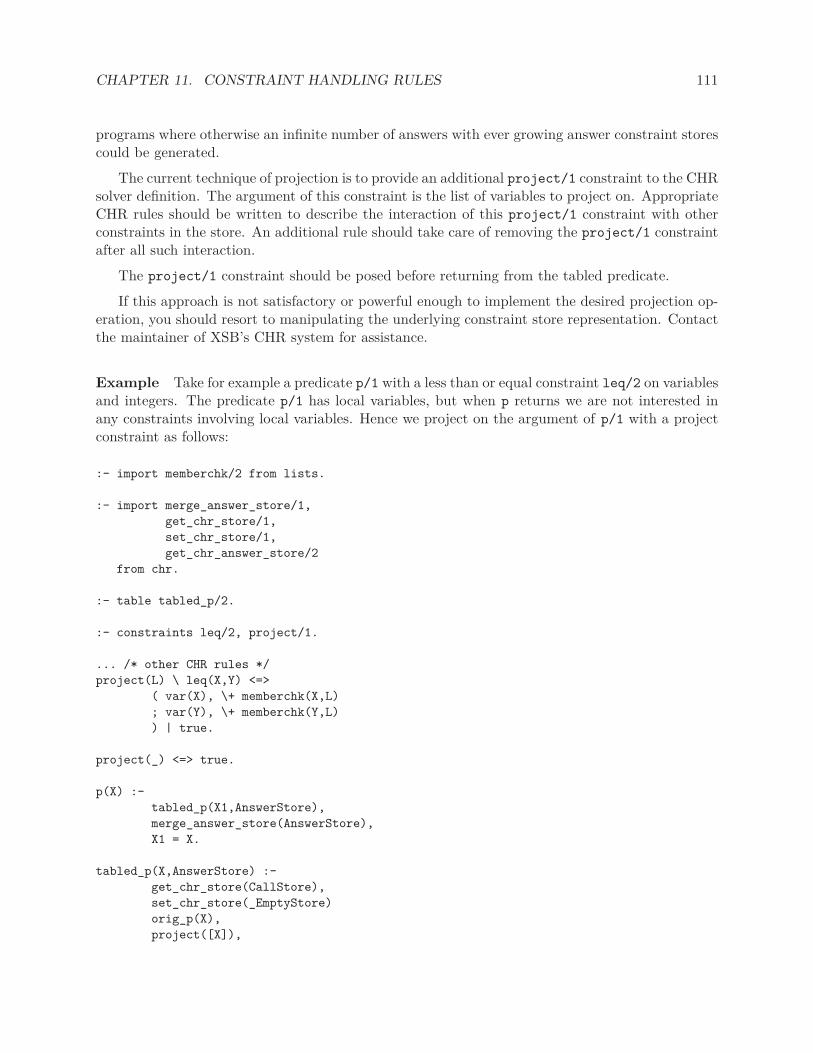
CHAPTER 11. CONSTRAINT HANDLING RULES 111
programs where otherwise an infinite number of answers with ever growing answer constraint storescould be generated.
The current technique of projection is to provide an additional project/1 constraint to the CHRsolver definition. The argument of this constraint is the list of variables to project on. AppropriateCHR rules should be written to describe the interaction of this project/1 constraint with otherconstraints in the store. An additional rule should take care of removing the project/1 constraintafter all such interaction.
The project/1 constraint should be posed before returning from the tabled predicate.
If this approach is not satisfactory or powerful enough to implement the desired projection op-eration, you should resort to manipulating the underlying constraint store representation. Contactthe maintainer of XSB’s CHR system for assistance.
Example Take for example a predicate p/1 with a less than or equal constraint leq/2 on variablesand integers. The predicate p/1 has local variables, but when p returns we are not interested inany constraints involving local variables. Hence we project on the argument of p/1 with a projectconstraint as follows:
:- import memberchk/2 from lists.
:- import merge_answer_store/1,
get_chr_store/1,
set_chr_store/1,
get_chr_answer_store/2
from chr.
:- table tabled_p/2.
:- constraints leq/2, project/1.
... /* other CHR rules */
project(L) \ leq(X,Y) <=>
( var(X), \+ memberchk(X,L)
; var(Y), \+ memberchk(Y,L)
) | true.
project(_) <=> true.
p(X) :-
tabled_p(X1,AnswerStore),
merge_answer_store(AnswerStore),
X1 = X.
tabled_p(X,AnswerStore) :-
get_chr_store(CallStore),
set_chr_store(_EmptyStore)
orig_p(X),
project([X]),

CHAPTER 11. CONSTRAINT HANDLING RULES 112
get_chr_answer_store(chrmod,AnswerStore),
set_chr_store(CallStore).
orig_p(X) :-
... /* original body of p/1 */.
The example in the following subsection shows projection in a full application.
11.6.4 Answer Combination
Sometimes it is desirable to combine different answers to a tabled predicate into one single answeror a subset of answers. Especially when otherwise there would be an infinite number of answers. Ifthe answers are expressed as constraints on some arguments and the logic of combining is encodedas CHR rules, answers can be combined by merging the respective answer constraint stores.
Another case where this is useful is when optimization is desired. If the answer to a predicaterepresents a valid solution, but an optimal solution is desired, the answer should be representedas constraints on arguments. By combining the answer constraints, only the most constrained, oroptimal, answer is kept.
Example An example of a program that combines answers for both termination and optimisationis the shortest path program below:
:- chr_module(path).
:- import length/2 from lists.
:- import merge_chr_answer_store/1,
get_chr_store/1,
set_chr_store/1,
get_chr_answer_store/2
from chr.
breg_retskel(A,B,C,D) :- ’_$builtin’(154).
:- constraints geq/2, plus/3, project/1.
geq(X,N) \ geq(X,M) <=> number(N), number(M), N =< M | true.
reflexivity @ geq(X,X) <=> true.
antisymmetry @ geq(X,Y), geq(Y,X) <=> X = Y.
idempotence @ geq(X,Y) \ geq(X,Y) <=> true.
transitivity @ geq(X,Y), geq(Y,Z) ==> var(Y) | geq(X,Z).
plus(A,B,C) <=> number(A), number(B) | C is A + B.
plus(A,B,C), geq(A,A1) ==> plus(A1,B,C1), geq(C,C1).
plus(A,B,C), geq(B,B1) ==> plus(A,B1,C1), geq(C,C1).

CHAPTER 11. CONSTRAINT HANDLING RULES 113
project(X) \ plus(_,_,_) # ID <=> true pragma passive(ID).
project(X) \ geq(Y,Z) # ID <=> (Y \== X ; var(Z) )| true pragma passive(ID).
project(_) <=> true.
path(X,Y,C) :-
tabled_path(X,Y,C1,AS),
merge_chr_answer_store(AS),
C = C1.
:- table tabled_path/4.
tabled_path(X,Y,C,AS) :-
’_$savecp’(Breg),
breg_retskel(Breg,4,Skel,Cs),
copy_term(p(X,Y,C,AS,Skel),p(OldX,OldY,OldC,OldAS,OldSkel)),
get_chr_store(GS),
set_chr_store(_GS1),
orig_path(X,Y,C),
project(C),
( get_returns(Cs,OldSkel,Leaf),
OldX == X, OldY == Y ->
merge_chr_answer_store(OldAS),
C = OldC,
get_chr_answer_store(path,MergedAS),
sort(MergedAS,AS),
( AS = OldAs ->
fail
;
delete_return(Cs,Leaf)
)
;
get_chr_answer_store(path,UnsortedAS),
sort(UnsortedAS,AS)
),
set_chr_store(GS).
orig_path(X,Y,C) :- edge(X,Y,C1), geq(C,C1).
orig_path(X,Y,C) :- path(X,Z,C2), edge(Z,Y,C1), plus(C1,C2,C0), geq(C,C0).
edge(a,b,1).
edge(b,a,1).
edge(b,c,1).
edge(a,c,3).
edge(c,a,1).
The predicate orig_path/3 specifies a possible path between two nodes in a graph. In tabled_path/4
multiple possible paths are combined together into a single path with the shortest distance. Hencethe tabling of the predicate will reject new answers that have a worse distance and will replace theold answer when a better answer is found. The final answer gives the optimal solution, the shortestpath. It is also necessary for termination to keep only the best answer. When cycles appear in the

CHAPTER 11. CONSTRAINT HANDLING RULES 114
graph, paths with longer and longer distance could otherwise be put in the table, contributing tothe generation of even longer paths. Failing for worse answers avoids this infinite build-up.
The predicate also includes a projection to remove constraints on local variables and only retainthe bounds on the distance.
The sorting canonicalizes the answer stores, so that they can be compared.
11.6.5 Overview of Tabling-related Predicates
merge_answer_store(+AnswerStore) chr
Merges the given CHR answer store into the current global CHR constraint store.
get_chr_store(-ConstraintStore) chr
Returns the current global CHR constraint store.
set_chr_store(?ConstraintStore) chr
Set the current global CHR constraint store. If the argument is a fresh variable, the currentglobal CHR constaint store is set to be an empty store.
get_chr_answer_store(+Mod,-AnswerStore) chr
Returns the part of the current global CHR constraint store of constraints in the specifiedCHR module, in the format of an answer store usable as a return argument of a tabledpredicate.
11.7 Guidelines
In this section we cover several guidelines on how to use CHR to write constraint solvers and howto do so efficiently.
• Set semantics: The CHR system allows the presence of identical constraints, i.e. multipleconstraints with the same functor, arity and arguments. For most constraint solvers, this isnot desirable: it affects efficiency and possibly termination. Hence appropriate simpagationrules should be added of the form:
constraint\constraint <=> true
• Multi-headed rules: Multi-headed rules are executed more efficiently when the constraintsshare one or more variables.
11.8 CHRd
An alternate implementation of CHR can be found in the CHRd package. The main objective ofthe CHRd package is to optimize processing of constraints in the environment where termination isguaranteed by the tabling engine, (and where termination benefits provided by the existing solver
CHAPTER 11. CONSTRAINT HANDLING RULES 115
are not critical). CHRd takes advantage of XSB’s tabling to simplify CHR’s underlying storagestructures and solvers. Specifically, we entirely eliminate the thread-global constraint store in favorof a distributed one, realized as a collection of sets of constraints entirely associated with programvariables. This decision limits the applicability of CHRd to a restricted class of CHR programs,refered to as direct-indexed CHR,in which all constraints in the head of a rule are connectedby shared variables. Most CHR programs are direct-indexed, and other programs may be easilyconverted to fall into this class. Another advance of CHRd is its set-based semantics which removesthe need to maintain the propagation history, thus allowing further simplicity in the representationof the constraints. The CHRd package itself is described in [22], and both the semantics of CHRdand the class of direct-indexed CHR are formally defined in [23].

Chapter 12
XASP: Answer Set Programmingwith XSB and Smodels
By Luis Castro, Terrance Swift, David S. Warren 1
The term Answer Set Programming (ASP) describes a paradigm in which logic programs areinterpreted using the (extended) stable model semantics. While the stable model semantics isquite elegant, it has radical differences from traditional program semantics based on Prolog. First,stable model semantics applies only to ground programs; second stable model semantics is notgoal-oriented – determining whether a stable model is true in a program involves examining eachclause in a program, regardless of whether the goal would depends on the clause in a traditionalevaluation 2.
Despite (or perhaps because of) these differences, ASP has proven to be a useful paradigmfor solving a variety of combinatorial programs. Indeed, determining a stable model for a logicprogram can be seen as an extension of the NP-complete problem of propositional satisfiability, sothat satisfiability problems that can be naturally represented as logic programs can be solved usingASP.
The current generation of ASP systems are very efficient for determining whether a program hasa stable model (analogous to whether the program, taken as a set of propositional axioms, is satisfi-able). However, ASP systems have somewhat primitive file-based interfaces. XSB is a natural com-plement to ASP systems. Its basis in Prolog provides a procedural counterpart for ASP, as describedin Chapter 5 of Volume 1 of this manual; and XSB’s computation of the Well-founded semanticshas a well-defined relationship to stable model semantics. Furthermore, deductive-database-likecapabilities of XSB allow it to be an efficient and flexible grounder for many ASP problems.
The XASP package provides various mechanisms that allow tight linkage of XSB programs tothe Smodels [20] stable model generator. The main interface is based on a store of clauses that can
1 Thanks to Barry Evans for helping resuscitate the XASP installation procedure, and to Gonçalo Lopes for theinstallation procedure on Windows.
2In Version 3.3, the Smodels API has not been tested with the multi-threaded engine, and Smodels itself is notthread-safe.
116

CHAPTER 12. XASP: ANSWER SET PROGRAMMING WITH XSB AND SMODELS 117
be incrementally asserted or deleted by an XSB program. Clauses in this store can make use of all ofthe cardinality and weight constraint syntax supported by Smodels, in addition to default negation.When the user decides that the clauses in a store are a complete representation of a program whosestable model should be generated, the clauses are copied into Smodels buffers. Using the SmodelsAPI, the generator is invoked, and information about any stable models generated are returned.This use of XASP is roughly analogous to building up a constraint store in CLP, and periodicallyevaluating that store, but integration with the store is less transparent in XASP than in CLP.In XASP, clauses must be explicitly added to a store and evaluated; furthermore clauses are notremoved from the store upon backtracking, unlike constraints in CLP.
The XNMR interpreter provides a second, somewhat more implicit use of XASP. In the XNMRinterface a query Q is evaluated as is any other query in XSB. However, conditional answersproduced for Q and for its subgoals, upon user request, can be considered as clauses and sentto Smodels for evaluation. In backtracking through answers for Q, the user backtracks not onlythrough answer substitutions for variables of Q, but also through the stable models produced forthe various bindings.
12.1 Installing the Interface
Installing the Smodels interface of XASP sometimes can be tricky for two reasons. First, XSBmust dynamically load the Smodels library, and dynamic loading introduces platform dependencies.Second since Smodels is written in C++ and XSB is written in C, the load must ensure that namesare properly resolved and that C++ libraries are loaded, steps that may addressed differently bydifferent compilers 3. However, by following the steps outlined below in the section for Unix orWindows, XASP should be running in a matter of minutes.
12.1.1 Installing the Interface under Unix
In order to use the Smodels interface, several steps must be performed.
1. Creating a library for Smodels. Smodels itself must be compiled as a library. Unlike previousversions of XSB, which required a special configuration step for Smodels, Version 3.3 requiresno special confiuration, since XSB includes source code for Smodels 2.33 as a subdirectoryof the $XSBDIR/packages/xasp directory (denoted $XASPDIR). We suggest making Smodelsout of this directory 4. Thus, to make the Smodels library
(a) Change directory to $XASPDIR/smodels
(b) On systems other than OS X, type
make lib
3XSB’s compiler can automatically call foreign compilers to compile modules written in C, but in Version 3.3 ofXSB C++ modules must be compiled with external commands, such as the make command shown below.
4Although distributed with XSB, Smodels is distributed under the GNU General Public License, a license that isslightly stricter than the license XSB uses. Users distributing applications based on XASP should be aware of anyrestrictions imposed by GNU General Public License.
CHAPTER 12. XASP: ANSWER SET PROGRAMMING WITH XSB AND SMODELS 118
on OS X, type 5
make -f Makefile.osx lib
If the compilation step ran successfully, there should be a file libsmodels.so (or libsomodels.dylib
on MacOS X or libsmodels.dll on Windows...) in $XASPDIR/smodels/.libs
(c) Change directory back to $XASPDIR
2. Compiling the XASP files Next, platform-specific compilation of XASP files needs to beperformed. This can be done by consulting prologMake.P and executing the goal
?- make.
It is important to note that under Version 3.3, code compiled by the single threaded engine willonly be executable by the single threaded engine, and code compiled by the multi-threadedengine will only be executable by the multi-threaded engine.
3. Checking the Installation To see if the installation is working properly, cd to the subdirectorytests and type:
sh testsuite.sh <$XSBDIR>
If the test suite succeeded it will print out a message along the lines of
PASSED testsuite for /Users/terranceswift/XSBNEW/XSB/config/powerpc-apple-darwin7.5.1/bin/xsb
12.1.2 Installing XASP under Windows using Cygwin
To install XASP under Windows, you must use Version 3.3 of XSB or later and Version 2.31 orlater of Smodels 6. You should also have a recent version of Cygwin (e.g. 1.5.20 or later) withall the relevant development packages installed, such as devel, make, automake, patchtools, andpossibly x11 (for makedepend) Without an appropriate Cygwin build environment many of thesesteps will simply fail, sometimes with quite cryptic error messages.
1. Patch and Compile Smodels First, uncompress smodels-2.31.tar.gz in some directory, (forpresentation purposes we use /cygdrive/c/smodels-2.31 — that is, c:\smodels-2.31).After that, you must apply the patch provided with this package. This patch enables thecreation of a DLL from Smodels. Below is a sample session (system output omitted) with therequired commands:
$ cd /cygdrive/c/smodels-2.31
$ cat $XSB/packages/xasp/patch-smodels-2.31 | patch -p1
$ make lib
5A special makefile is needed for OS X since the GNU libtool is called glibtool on this platform.6This section was written by Goncalo Lopes.

CHAPTER 12. XASP: ANSWER SET PROGRAMMING WITH XSB AND SMODELS 119
After that, you should have a file called smodels.dll in the current directory, as well as a filecalled smodels.a. You should make the former "visible" to Windows. Two alternatives areeither (a) change the PATH environment variable to contain c:\smodels-2.31, or (b) copysmodels.dll to some other directory in your PATH (such as c:\windows, for instance). Onesimple way to do this is to copy smodels.dll to $XSB/config/i686-pc-cygwin/bin, afterthe configure XSB step (step 2), since that directory has to be in your path in order to makeXSB fully functional.
2. Configure XSB. In order to properly configure XSB, you must tell it where the Smodelssources and library (the smodels.a file) are. In addition, you must compile XSB such thatit doesn’t use the Cygwin DLL (using the -mno-cygwin option for gcc). The following is asample command:
$ cd $XSB/build
$ ./configure --enable-no-cygwin -with-smodels="/cygdrive/c/smodels-2.31’’
You can optionally include the extended Cygwin w32 API using the configuration option--with-includes=<PATH_TO_API>, (this allows XSB’s build procedure to find makedepend
for instance), but you’ll probably do fine with just the standard Cygwin apps.
There are some compiler variables which may not be automatically set by the configure scriptin xsb_config.h, namely the configuration names and some activation flags. To correct this,do the following:
(a) cd to $XSB/config/i686-pc-cygwin
(b) open the file xsb_config.h and add the following lines:
#define CONFIGURATION "i686-pc-cygwin"
#define FULL_CONFIG_NAME "i686-pc-cygwin"
#define SLG_GC
(Still more flags may be needed depending on Cygwin configuration)
After applying these changes, cd back to the $XSB/build directory and compile XSB:
$ ./makexsb
Now you should have in $XSB/config/i686-pc-cygwin/bin directory both a xsb.exe anda xsb.dll.
3. Compiling XASP. First, go to the XASP directory and execute the makelinks.sh script inorder to make the headers and libraries in Smodels be accessible to XSB, i.e.:
$ cd $XSB/packages/xasp
$ sh makelinks.sh /cygdrive/c/smodels-2.31
Now you must copy the smoMakefile from the config directory to the xasp directory andrun both its directives:

CHAPTER 12. XASP: ANSWER SET PROGRAMMING WITH XSB AND SMODELS 120
$ cp $XSB/config/i686-pc-cygwin/smoMakefile .
$ make -f smoMakefile module
$ make -f smoMakefile all
At this point, you can consult xnmr as you can with any other package, or xsb with thexnmr command line parameter, like this: (don’t forget to add XSB bin directory to the $PATH
environment variable)
$ xsb xnmr
Lots of error messages will probably appear because of some runtime load compiler, but ifeverything goes well you can ignore all of them since your xasppkg will be correctly loadedand everything will be functioning smoothly from there on out.
12.2 The Smodels Interface
The Smodels interface contains two levels: the cooked level and the raw level. The cooked levelinterns rules in an XSB clause store, and translates general weight constraint rules [24] into a normalform that the Smodels engine can evaluate. When the programmer has determined that enoughclauses have been added to the store to form a semantically complete sub-program, the programis committed. This means that information in the clauses is copied to Smodels and interned usingSmodels data structures so that stable models of the clauses can be computed and examined. Byconvention, the cooked interface ensures that the atom true is present in all stable models, andthe atom false is false in all stable models. The raw level models closely the Smodels API, anddemands, among other things, that each atom in a stable sub-program has been translated into aunique integer. The raw level also does not provide translation of arbitrary weight constraint rulesinto the normal form required by the Smodels engine. As a result, the raw level is significantlymore difficult to directly use than the cooked level. While we make public the APIs for both theraw and cooked level, we provide support only for users of the cooked interface.
As mentioned above Smodels extends normal programs to allow weight constraints, which canbe useful for combinatorial problems. However, the syntax used by Smodels for weight constraintsdoes not follow ISO Prolog syntax so that the XSB syntax for weight constraints differs in somerespects from that of Smodels. Our syntax is defined as follows, where A is a Prolog atom, N anon-negative integer, and I an arbitrary integer.
• GeneralLiteral ::= WeightConstraint | Literal
• WeightConstraint ::= weightConst(Bound,WeightList,Bound)
• WeightList ::= List of WeightLiterals
• WeightLiteral ::= Literal | weight(Literal,N)
• Literal ::= A | not(A)

CHAPTER 12. XASP: ANSWER SET PROGRAMMING WITH XSB AND SMODELS 121
• Bound ::== I | undef
Thus an example of a weight constraint might be:
• weightConst(1,[weight(a,1),weight(not(b),1)],2)
We note that if a user does not wish to put an upper or lower bound on a weight constraint, shemay simply set the bound to undef or to an integer less than 0.
The intuitive semantics of a weight constraint weightConst(Lower,WeightList,Upper), inwhich List is is list of WeightLiterals that it is true in a model M whenever the sum of the weightsof the literals in the constraint that are true in M is between the lower Lower and Upper. Anyliteral in a WeightList that does not have a weight explicitly attached to it is taken to have a weightof 1.
In a typical session, a user will initialize the Smodels interface, add rules to the clause store untilit contains a semantically meaningful sub-problem. He can then specify a compute statement ifneeded, commit the rules, and compute and examine stable models via backtracking. If desired, theuser can then re-initialize the interface, and add rules to or retract rules from the clause store untilanother semantically meaningful sub-program is defined; and then commit, compute and examineanother stable model 7.
The process of adding information to a store and periodically evaluating it is vaguely reminiscentof the Constraint Logic Programming (CLP) paradigm, but there are important differences. InCLP, constraints are part of the object language of a Prolog program: constraints are added to orprojected out of a constraint store upon forward execution, removed upon backwards execution, anditeratively checked. When using this interface, on the other hand, an XSB program essentially actsas a compiler for the clause store, which is treated as a target language. Clauses must be explicitlyadded or removed from the store, and stable model computation cannot occur incrementally –it must wait until all clauses have been added to the store. We note in passing that the xnmr
module provides an elegant but specialized alternative. xnmr integrates stable models into theobject language of XSB, by computing ""relevant"" stable models from the the residual answersproduced by query evaluation. It does not however, support the weighted constraint rules, computestatements and so on that this module supports.
Neither the raw nor the cooked interface currently supports explicit negation.
Examples of use of the various interfaces can be found in the subdirectory intf_examples
smcInit
Initializes the XSB clause store and the Smodels API. This predicate must be executed beforebuilding up a clause store for the first time. The corresponding raw predicate, smrInit(Num),initializes the Smodels API assuming that it will require at most Num atoms.
smcReInit
Reinitializes the Smodels API, but does not affect the XSB clause store. This predicate is
7Currently, only normal rules can be retracted.

CHAPTER 12. XASP: ANSWER SET PROGRAMMING WITH XSB AND SMODELS 122
provided so that a user can reuse rules in a clause store in the context of more than onesub-program.
smcAddRule(+Head,+Body)
Interns a ground rule into the XSB clause store. Head must be a GeneralLiteral as definedat the beginning of this section, and Body must be a list of GeneralLiterals. Upon interning,the rule is translated into a normal form, if necessary, and atoms are translated to uniqueintegers. The corresponding raw predicates, smrAddBasicRule/3, smrAddChoiceRule/3,smrAddConstraintRule/4, and smrAddWeightRule/3 can be used to add raw predicates im-mediately into the SModels API.
smcRetractRule(+Head,+Body)
Retracts a ground (basic) rule from the XSB clause store. Currently, this predicate cannotretract rules with weight constraints: Head must be a Literal as defined at the beginning ofthis section, and Body must be a list of GeneralLiterals.
smcSetCompute(+List)
Requires that List be a list of literals – i.e. atoms or the default negation of atoms). Thispredicate ensures that each literal in List is present in the stable models returned by Smodels.By convention the cooked interface ensures that true is present and false absent in all stablemodels. After translating a literal it calls the raw interface predicates smrSetPosCompute/1
and smrSetNegCompute/1
smcCommitProgram
This predicate translates all of the clauses from the XSB clause store into the data structuresof the Smodels API. It then signals to the API that all clauses have been added, and initializesthe Smodels computation. The corresponding raw predicate, smrCommitProgram, performsonly the last two of these features.
smComputeModel
This predicate calls Smodels to compute a stable model, and succeeds if a stable modelcan be computed. Upon backtracking, the predicate will continue to succeed until all stablemodels for a given program cache have been computed. smComputeModel/0 is used by boththe raw and the cooked levels.
smcExamineModel(+List,-Atoms)
smcExamineModel/(+List,-Atoms) filters the literals in List to determine which are true inthe most recently computed stable model. These true literals are returned in the list Atoms.smrExamineModel(+N,-Atoms) provides the corresponding raw interface in which integersfrom 0 to N, true in the most recently computed stable model, are input and output.
smEnd
Reclaims all resources consumed by Smodels and the various APIs. This predicate is usedby both the cooked and the raw interfaces.
print_cache
This predicate can be used to examine the XSB clause store, and may be useful for debugging.
CHAPTER 12. XASP: ANSWER SET PROGRAMMING WITH XSB AND SMODELS 123
12.2.1 Using the Smodels Interface with Multiple Threads
If XASP has been compiled under the multi-threaded engine, the Smodels interface will be fullythread-safe: this means that Smodels and all interface predicates described in this section can beused concurrently by different threads. In multi-threaded XASP, each XSB thread can initializeand query its own instance of Smodels, and build up its own private clause store at both the cookedand raw levels (shared clause stores are not yet available). Figure 12.1 provides a simple exampleof how this can be done. For each thread that will generate stable models, a message queue iscreated that will be used to communicate back results. Two threads are then created and thesethreads concurrently add rules to their private clause stores, call Smodels, and send the resultsback to the calling thread using the appropriate message queue. Of course the example here is justone of many possible: answers could be returned using different configurations of message queues,through shared tables, through shared asserted code, and so on.
12.3 The xnmr_int Interface
. This module provides the interface from the xnmr module to Smodels. It does not use thesm_int interface, but rather directly calls the Smodels C interface, and can be thought of as aspecial-purpose alternative to sm_int.
init_smodels(+Query)
Initializes smodels with the residual program produced by evaluating Query. Query must bea call to a tabled predicate that is currently completely evaluated (and should have a delaylist)
atom_handle(?Atom,?AtomHandle)
The handle of an atom is set by init_smodels/1 to be an integer uniquely identifying eachatoms in the residual program (and thus each atom in the Herbrand base of the program forwhich the stable models are to be derived). The initial query given to init_smodels has theatom-handle of 1.
in_all_stable_models(+AtomHandle,+Neg)
in_all_stable_models/2 returns true if Neg is 0 and the atom numbered AtomHandle re-turns true in all stable models (of the residual program set by the previous call to init_smodels/1).If Neg is nonzero, then it is true if the atom is in NO stable model.
pstable_model(+Query,-Model,+Flag)
returns nondeterministically a list of atoms true in the partial stable model total on theatoms relevant to instances of Query, if Flag is 0. If Flag is 1, it only returns models inwhich the instance of Query is true.
a_stable_model
This predicate invokes Smodels to find a (new) stable model (of the program set by the previ-ous invocation of init_smodels/1.) It will compute all stable models through backtracking.If there are no (more) stable models, it fails. Atoms true in a stable model can be examinedby in_current_stable_model/1.
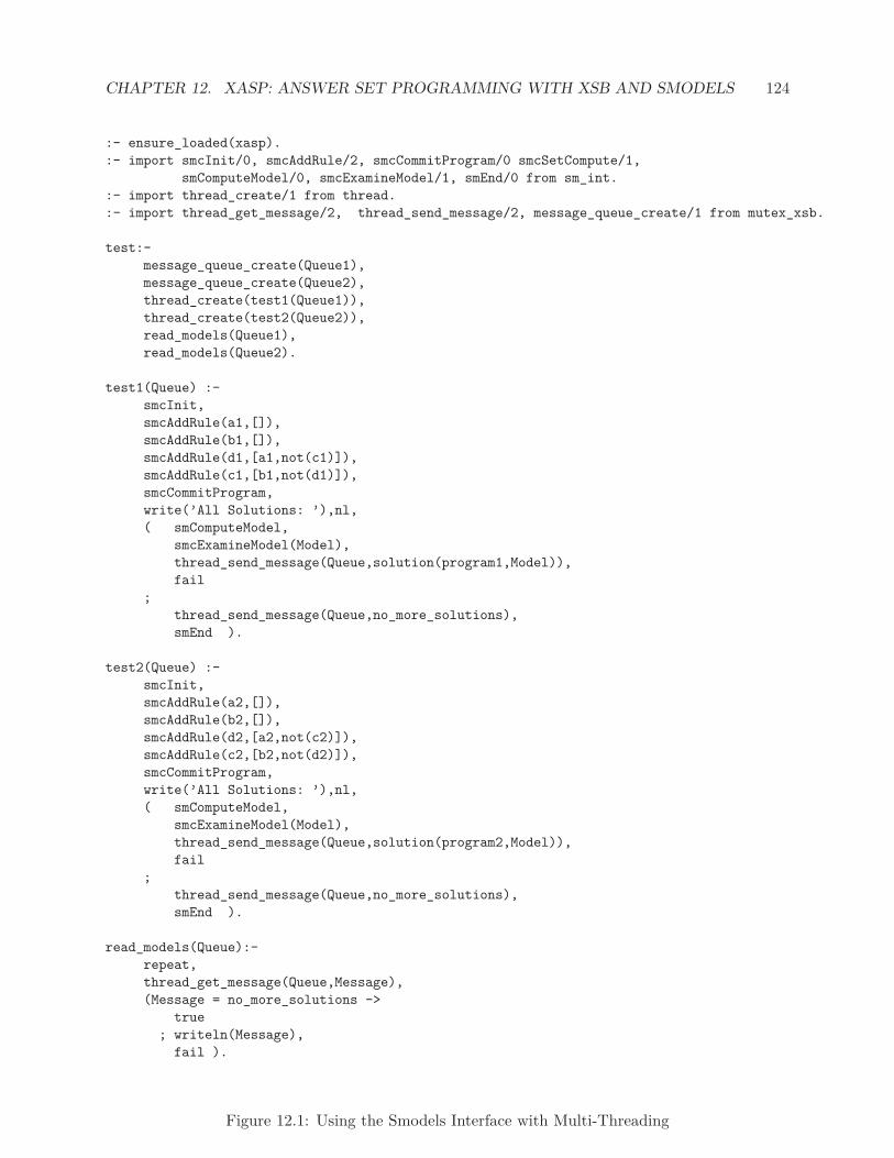
CHAPTER 12. XASP: ANSWER SET PROGRAMMING WITH XSB AND SMODELS 124
:- ensure_loaded(xasp).
:- import smcInit/0, smcAddRule/2, smcCommitProgram/0 smcSetCompute/1,
smComputeModel/0, smcExamineModel/1, smEnd/0 from sm_int.
:- import thread_create/1 from thread.
:- import thread_get_message/2, thread_send_message/2, message_queue_create/1 from mutex_xsb.
test:-
message_queue_create(Queue1),
message_queue_create(Queue2),
thread_create(test1(Queue1)),
thread_create(test2(Queue2)),
read_models(Queue1),
read_models(Queue2).
test1(Queue) :-
smcInit,
smcAddRule(a1,[]),
smcAddRule(b1,[]),
smcAddRule(d1,[a1,not(c1)]),
smcAddRule(c1,[b1,not(d1)]),
smcCommitProgram,
write(’All Solutions: ’),nl,
( smComputeModel,
smcExamineModel(Model),
thread_send_message(Queue,solution(program1,Model)),
fail
;
thread_send_message(Queue,no_more_solutions),
smEnd ).
test2(Queue) :-
smcInit,
smcAddRule(a2,[]),
smcAddRule(b2,[]),
smcAddRule(d2,[a2,not(c2)]),
smcAddRule(c2,[b2,not(d2)]),
smcCommitProgram,
write(’All Solutions: ’),nl,
( smComputeModel,
smcExamineModel(Model),
thread_send_message(Queue,solution(program2,Model)),
fail
;
thread_send_message(Queue,no_more_solutions),
smEnd ).
read_models(Queue):-
repeat,
thread_get_message(Queue,Message),
(Message = no_more_solutions ->
true
; writeln(Message),
fail ).
Figure 12.1: Using the Smodels Interface with Multi-Threading
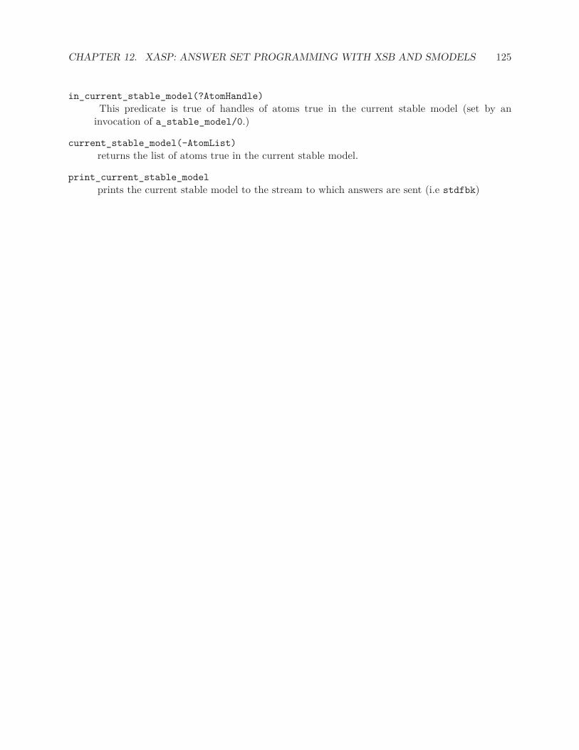
CHAPTER 12. XASP: ANSWER SET PROGRAMMING WITH XSB AND SMODELS 125
in_current_stable_model(?AtomHandle)
This predicate is true of handles of atoms true in the current stable model (set by aninvocation of a_stable_model/0.)
current_stable_model(-AtomList)
returns the list of atoms true in the current stable model.
print_current_stable_model
prints the current stable model to the stream to which answers are sent (i.e stdfbk)

Chapter 13
PITA: Probabilistic Inference withTabling and Answer subsumption
By Fabrizio Riguzzi
“Probabilistic Inference with Tabling and Answer subsumption” (PITA) [21] is a package foruncertain reasoning. In particular, it allowsvarious forms of Probabilistic Logic Programmingand Possibilistic Logic Programming. It accepts the language of Logic Programs with AnnotatedDisjunctions (LPADs)[28, 29] and CP-logic programs [26, 27].
An example of LPAD/CP-logic program is
(heads(Coin) : 0.5) ∨ (tails(Coin) : 0.5) ← toss(Coin),¬biased(Coin).
(heads(Coin) : 0.6) ∨ (tails(Coin) : 0.4) ← toss(Coin), biased(Coin).
(fair(Coin) : 0.9) ∨ (biased(Coin) : 0.1).
toss(Coin).
The first clause states that if we toss a coin that is not biased it has equal probability of landingheads and tails. The second states that if the coin is biased it has a slightly higher probability oflanding heads. The third states that the coin is fair with probability 0.9 and biased with probability0.1 and the last clause states that we toss a coin with certainty.
PITA computes the probability of queries by tranforming the input program into a normal logicprogram and then calling a modified version of the query on the transformed programs.
13.0.1 Installation
PITA uses GLib 2.0 and CUDD. GLib is a standard GNU package so it is easy to install it usingthe package management software of your Linux distribution.
To install CUDD, follow the instructions at http://vlsi.colorado.edu/~fabio/CUDD/ toget the package (or get directly from ftp://vlsi.colorado.edu/pub/cudd-2.4.2.tar.gz), for
126

CHAPTER 13. PITA: PROBABILISTIC INFERENCE WITH TABLING AND ANSWER SUBSUMPTION 127
example cudd-2.4.2.tar.gz. After decompressing, you will have a direcory cudd-2.4.2 withvarious subdirectories. Compile CUDD following the included instructions.
To install PITA with XSB, run XSB configure in the build directory with option –with-pita=DIR
where DIR is the folder where CUDD is.
Syntax
Disjunction in the head is represented with a semicolon and atoms in the head are separated fromprobabilities by a colon. For the rest, the usual syntax of Prolog is used. For example, the CP-logicclause
h1 : p1 ∨ . . . ∨ hn : pn ← b1, . . . , bm,¬c1, . . . ,¬cl
is represented by
h1:p1 ; ... ; hn:pn :- b1,...,bm,\+ c1,....,\+ cl
No parentheses are necessary. The pi are numeric expressions. It is up to the user to ensure thatthe numeric expressions are legal, i.e. that they sum up to less than one.
If the clause has an empty body, it can be represented like this
h1:p1 ; ... ;hn:pn.
If the clause has a single head with probability 1, the annotation can be omitted and the clausetakes the form of a normal prolog clause, i.e.
h1:- b1,...,bm,\+ c1,...,\+ cl.
stands for
h1:1 :- b1,...,bm,\+ c1,...,\+ cl.
The body of clauses can contain a number of built-in predicates including:
is/2 >/2 </2 >=/2 =</2 =:=/2 =\=/2 true/0 false/0
=/2 ==/2 \=/2 \==/2 length/2 member/2
The coin example above thus is represented as (see file coin.cpl in subdirecoty examples)
heads(Coin):1/2 ; tails(Coin):1/2:-
toss(Coin),\+biased(Coin).
heads(Coin):0.6 ; tails(Coin):0.4:-
toss(Coin),biased(Coin).
fair(Coin):0.9 ; biased(Coin):0.1.
toss(coin).
Subdirectory examples contains other example programs.
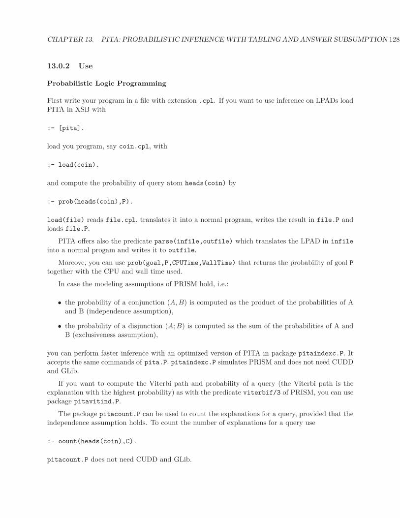
CHAPTER 13. PITA: PROBABILISTIC INFERENCE WITH TABLING AND ANSWER SUBSUMPTION 128
13.0.2 Use
Probabilistic Logic Programming
First write your program in a file with extension .cpl. If you want to use inference on LPADs loadPITA in XSB with
:- [pita].
load you program, say coin.cpl, with
:- load(coin).
and compute the probability of query atom heads(coin) by
:- prob(heads(coin),P).
load(file) reads file.cpl, translates it into a normal program, writes the result in file.P andloads file.P.
PITA offers also the predicate parse(infile,outfile) which translates the LPAD in infile
into a normal progam and writes it to outfile.
Moreove, you can use prob(goal,P,CPUTime,WallTime) that returns the probability of goal P
together with the CPU and wall time used.
In case the modeling assumptions of PRISM hold, i.e.:
• the probability of a conjunction (A, B) is computed as the product of the probabilities of Aand B (independence assumption),
• the probability of a disjunction (A; B) is computed as the sum of the probabilities of A andB (exclusiveness assumption),
you can perform faster inference with an optimized version of PITA in package pitaindexc.P. Itaccepts the same commands of pita.P. pitaindexc.P simulates PRISM and does not need CUDDand GLib.
If you want to compute the Viterbi path and probability of a query (the Viterbi path is theexplanation with the highest probability) as with the predicate viterbif/3 of PRISM, you can usepackage pitavitind.P.
The package pitacount.P can be used to count the explanations for a query, provided that theindependence assumption holds. To count the number of explanations for a query use
:- oount(heads(coin),C).
pitacount.P does not need CUDD and GLib.
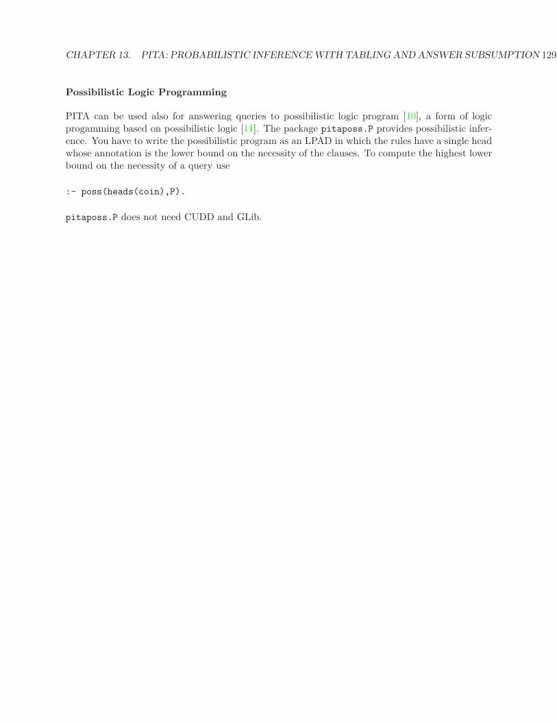
CHAPTER 13. PITA: PROBABILISTIC INFERENCE WITH TABLING AND ANSWER SUBSUMPTION 129
Possibilistic Logic Programming
PITA can be used also for answering queries to possibilistic logic program [10], a form of logicprogamming based on possibilistic logic [11]. The package pitaposs.P provides possibilistic infer-ence. You have to write the possibilistic program as an LPAD in which the rules have a single headwhose annotation is the lower bound on the necessity of the clauses. To compute the highest lowerbound on the necessity of a query use
:- poss(heads(coin),P).
pitaposs.P does not need CUDD and GLib.

Chapter 14
Other XSB Packages
Many of the XSB packages are maintained somewhat independently of XSB and have their ownmanuals. For these packages: Flora2, XMC, xsbdoc and Cold Dead Fish we provide summaries; fullinformation can be obtained in the packages themselves. In addition, we provide full documentationhere for two of the smaller packages, slx and GAP.
14.1 Programming with FLORA-2
Flora-2 is a sophisticated object-oriented knowledge base language and application developmentplatform. It is implemented as a set of run-time libraries and a compiler that translates a unifiedlanguage of F-logic [16], HiLog [7], and Transaction Logic [4, 3] into tabled Prolog code.
Applications of Flora-2 include intelligent agents, Semantic Web, ontology management, in-tegration of information, and others.
The programming language supported by Flora-2 is a dialect of F-logic with numerous ex-tensions, which include a natural way to do meta-programming in the style of HiLog and logicalupdates in the style of Transaction Logic. Flora-2 was designed with extensibility and flexibilityin mind, and it provides strong support for modular software design through its unique feature ofdynamic modules. Other extensions, such as the versatile syntax of Florid path expressions, areborrowed from Florid, a C++-based F-logic system developed at Freiburg University.1 Extensionsaside, the syntax of Flora-2 differs in many important ways from Florid, from the original ver-sion of F-logic, as described in [16], and from an earlier implementation of Flora. These syntacticchanges were needed in order to bring the syntax of Flora-2 closer to that of Prolog and make itpossible to include simple Prolog programs into Flora-2 programs without choking the compiler.Other syntactic deviations from the original F-logic syntax are a direct consequence of the addedsupport for HiLog, which obviates the need for the “@” sign in method invocations (this sign isnow used to denote calls to Flora-2 modules).
Flora-2 is distributed in two ways. First, it is part of the official distribution of XSB andthus is installed together with XSB. Second, a more up-to-date version of the system is available
1 See http://www.informatik.uni-freiburg.de/∼dbis/florid/ for more details.
130

CHAPTER 14. OTHER XSB PACKAGES 131
on Flora-2 ’s Web site at
http://flora.sourceforge.net
These two versions can be installed at the same time and used independently (e.g., if you want tokeep abreast with the development of Flora-2 or if a newer version was released in-between thereleases of XSB). The installation instructions are somewhat different in these two cases. Here weonly describe the process of configuring the version Flora-2 included with XSB.
Installing Flora-2 under UNIX. To configure a version of Flora-2 that was downloadedas part of the distribution of XSB, simply configure XSB as usual:
cd XSB/build
configure
makexsb
and then run
makexsb packages
If you downloaded XSB from its CVS repository earlier and are updating your copy using thecvs update command, then it might be a good idea to also do the following:
cd packages/flora2
makeflora clean
makeflora
Installing Flora-2 in Windows. First, you need Microsoft’s nmake. Then use the followingcommands to configure Flora-2 (assuming that XSB is already installed and configured):
cd flora2
makeflora clean
makeflora path-to-prolog-executable
Also make sure that the packages directory contains a shortcut called flora2.P to the filepackages\flora2\flora2.P.
Running Flora-2 . Flora-2 is fully integrated into the underlying XSB engine, including itsmodule system. In particular, Flora-2 modules can invoke predicates defined in other Prologmodules, and Prolog modules can query the objects defined in Flora-2 modules.
Due to certain problems with XSB, Flora-2 runs best when XSB is configured with localscheduling, which is the default XSB configuration. However, with this type of scheduling, manyProlog intuitions that relate to the operational semantics do not work. Thus, the programmer

CHAPTER 14. OTHER XSB PACKAGES 132
must think “more declaratively” and, in particular, to not rely on the order in which answers arereturned.
The easiest way to get a feel of the system is to start Flora-2 shell and begin to enter queriesinteractively. The simplest way to do this is to use the shell script
.../flora2/runflora
where “...” is the directory where Flora-2 is downloaded. For instance, to invoke the versionsupplied with XSB, you would type something like
~/XSB/packages/flora2/runflora
At this point, Flora-2 takes over and F-logic syntax becomes the norm. To get back to theProlog command loop, type Control-D (Unix) or Control-Z (Windows), or
| ?- _end.
If you are using Flora-2 shell frequently, it pays to define an alias, say (in Bash):
alias runflora=’~/XSB/packages/flora2/runflora’
Flora-2 can then be invoked directly from the shell prompt by typing runflora. It is evenpossible to tell Flora-2 to execute commands on start-up. For instance,
foo> runflora -e "_help."
will cause the system to execute the help command right after after the initialization. Then theusual Flora-2 shell prompt is displayed.
Flora-2 comes with a number of demo programs that live in
.../flora2/demos/
The demos can be run issuing the command “_demo(demo-filename).” at the Flora-2 prompt,e.g.,
flora2 ?- _demo(flogic_basics).
There is no need to change to the demo directory, as flDemo knows where to find these programs.
14.2 Summary of xmc: Model-checking with XSB
No documentation yet available.

CHAPTER 14. OTHER XSB PACKAGES 133
the Ciao [6] system’s lpdoc which has been adapted to generate a reference manual automaticallyfrom one or more XSB source files. The target format of the documentation can be Postscript,HTML, PDF, or nicely formatted ASCII text. xsbdoc can be used to automatically generate adescription of full applications, library modules, README files, etc. A fundamental advantage ofusing xsbdoc to document programs is that it is much easier to maintain a true correspondencebetween the program and its documentation, and to identify precisely to what version of theprogram a given printed manual corresponds. Naturally, the xsbdoc manual is generated by xsbdoc
itself.
The quality of the documentation generated can be greatly enhanced by including within theprogram text:
• assertions (indicating types, modes, etc. ...) for the predicates in the program, via thedirective pred/1; and
• machine-readable comments (in the “literate programming” style).
The assertions and comments included in the source file need to be written using the forthcomingXSB assertion language, which supports most of the features of Ciao’s assertion language within asimple and (hopefully) intuitive syntax.
xsbdoc is distributed under the GNU general public license.
Unlike lpdoc, xsbdoc does not use Makefiles, and instead maintains information about how togenerate a document within Prolog format files. As a result, xsbdoc can in principle be run in anyenvironment that supports the underlying software, such as XSB, LATEX, dvips and so on. It hasbeen tested on Linux and Windows running with Cygwin.
14.3 slx: Extended Logic Programs under the Well-Founded Se-mantics
As explained in the section Using Tabling in XSB, XSB can compute normal logic programs accord-ing to the well-founded semantics. In fact, XSB can also compute Extended Logic Programs, whichcontain an operator for explicit negation (written using the symbol -) in addition to the negation-by-failure of the well-founded semantics (\+ or not). Extended logic programs can be extremelyuseful when reasoning about actions, for model-based diagnosis, and for many other uses [2]. Thelibrary, slx provides a means to compile programs so that they can be executed by XSB accord-ing to the well-founded semantics with explicit negation [1]. Briefly, WFSX is an extension of thewell-founded semantics to include explicit negation and which is based on the coherence principlein which an atom is taken to be default false if it is proven to be explicitly false, intuitively:
−p⇒ not p.
This section is not intended to be a primer on extended logic programming or on WFSXsemantics, but we do provide a few sample programs to indicate the action of WFSX. Consider theprogram
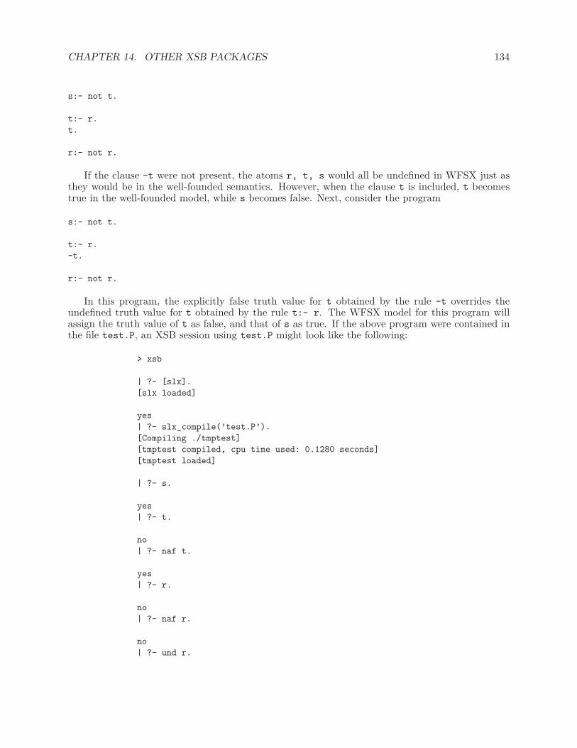
CHAPTER 14. OTHER XSB PACKAGES 134
s:- not t.
t:- r.
t.
r:- not r.
If the clause -t were not present, the atoms r, t, s would all be undefined in WFSX just asthey would be in the well-founded semantics. However, when the clause t is included, t becomestrue in the well-founded model, while s becomes false. Next, consider the program
s:- not t.
t:- r.
-t.
r:- not r.
In this program, the explicitly false truth value for t obtained by the rule -t overrides theundefined truth value for t obtained by the rule t:- r. The WFSX model for this program willassign the truth value of t as false, and that of s as true. If the above program were contained inthe file test.P, an XSB session using test.P might look like the following:
> xsb
| ?- [slx].
[slx loaded]
yes
| ?- slx_compile(’test.P’).
[Compiling ./tmptest]
[tmptest compiled, cpu time used: 0.1280 seconds]
[tmptest loaded]
| ?- s.
yes
| ?- t.
no
| ?- naf t.
yes
| ?- r.
no
| ?- naf r.
no
| ?- und r.
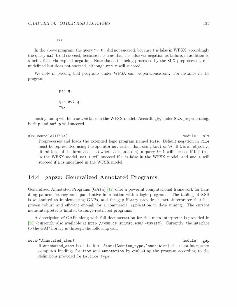
CHAPTER 14. OTHER XSB PACKAGES 135
yes
In the above program, the query ?- t. did not succeed, because t is false in WFSX: accordinglythe query naf t did succeed, because it is true that t is false via negation-as-failure, in addition tot being false via explicit negation. Note that after being processed by the SLX preprocessor, r isundefined but does not succeed, although und r will succeed.
We note in passing that programs under WFSX can be paraconsistent. For instance in theprogram.
p:- q.
q:- not q.
-q.
both p and q will be true and false in the WFSX model. Accordingly, under SLX preprocessing,both p and naf p will succeed.
slx_compile(+File) module: slx
Preprocesses and loads the extended logic program named File. Default negation in File
must be represented using the operator not rather than using tnot or \+. If L is an objectiveliteral (e.g. of the form A or −A where A is an atom), a query ?- L will succeed if L is truein the WFSX model, naf L will succeed if L is false in the WFSX model, and und L willsucceed if L is undefined in the WFSX model.
14.4 gapza: Generalized Annotated Programs
Generalized Annotated Programs (GAPs) [17] offer a powerful computational framework for han-dling paraconsistency and quantitative information within logic programs. The tabling of XSBis well-suited to implementing GAPs, and the gap library provides a meta-interpreter that hasproven robust and efficient enough for a commercial application in data mining. The currentmeta-interpreter is limited to range-restricted programs.
A description of GAPs along with full documentation for this meta-interpreter is provided in[25] (currently also available at http://www.cs.sunysb.edu/∼tswift). Currently, the interfaceto the GAP library is through the following call.
meta(?Annotated_atom) module: gap
If Annotated_atom is of the form Atom:[Lattice_type,Annotation] the meta-interpretercomputes bindings for Atom and Annotation by evaluating the program according to thedefinitions provided for Lattice_type.

Bibliography
[1] J. Alferes, C. Damasio, and L. Pereira. A logic programming system for non-monotonic rea-soning. Journal of Automated Reasoning, 1995.
[2] J. Alferes and L. M. Pereira. Reasoning with Logic Programming, volume 1111. Springer-VerlagLNAI, 1996.
[3] A. Bonner and M. Kifer. An overview of transaction logic. Theoretical Computer Science,133:205–265, October 1994.
[4] A. Bonner and M. Kifer. A logic for programming database transactions. In J. Chomicki andG. Saake, editors, Logics for Databases and Information Systems, chapter 5, pages 117–166.Kluwer Academic Publishers, March 1998.
[5] G. Box and M. Muller. A note on the generation of random normal deviates. The Annals ofMathematical Statistics, 29(2):610–611, 1958.
[6] F. Bueno, D. Cabenza, M. Carro, M. Hermenegildo, P. López-García, and G. Puebla. Theciao prolog system, reference manual. Technical report, School of Computer Science, TechnicalUniversity of Madrid, 2003. Available from http://www.clip.dia.fi.upm.es/.
[7] W. Chen, M. Kifer, and D. Warren. HiLog: A foundation for higher-order logic programming.Journal of Logic Programming, 15(3):187–230, February 1993.
[8] B. Demoen. Dynamic attributes, their hProlog implementation, and a first evaluation. ReportCW 350, Department of Computer Science, K.U.Leuven, Leuven, Belgium, oct 2002. URL =http://www.cs.kuleuven.ac.be/publicaties/rapporten/cw/CW350.abs.html.
[9] C. Draxler. Prolog to SQL compiler, Version 1.0. Technical report, CIS Centre for Informationand Speech Processing Ludwig-Maximilians-University, Munich, 1992.
[10] D. Dubois, J. Lang, and H. Prade. Towards possibilistic logic programming. In ICLP, pages581–595, 1991.
[11] D. Dubois, J. Lang, and H. Prade. Possibilistic logic. In D. M. Gabbay, C. J. Hogger, andJ. A. Robinson, editors, Handbook of logic in artificial intelligence and logic programming,vol.3, pages 439–514. Oxford University Press, 1994.
[12] T. Fruehwirth. Thom Fruehwirth’s Constraint Handling Rules website.http://www.informatik.uni-ulm.de/pm/mitarbeiter/fruehwirth/chr-intro.html.
136

BIBLIOGRAPHY 137
[13] T. Frühwirth. Theory and Practice of Constraint Handling Rules. In P. Stuckey and K. Marriot,editors, Special Issue on Constraint Logic Programming, volume 37, October 1998.
[14] H. Guo, C. R. Ramakrishnan, and I. V. Ramakrishnan. Speculative beats conservative justi-fication. In International Conference on Logic Programming, volume 2237 of Lecture Notes inComputer Science, pages 150–165. Springer, 2001.
[15] C. Holzbaur. Ofai clp(q,r) manual, edition 1.3.3. Technical report, Austrian Research Institutefor Artificial Intelligence, 1995.
[16] M. Kifer, G. Lausen, and J. Wu. Logical foundations of object-oriented and frame-basedlanguages. Journal of the ACM, 42:741–843, July 1995.
[17] M. Kifer and V. S. Subrahmanian. Theory of generalized annotated logic programming andits applications. J. Logic Programming, 12(4):335–368, 1992.
[18] T. I. S. Laboratory. SICStus Prolog User’s Manual Version 3.12.5. Swedish Institute ofComputer Science, 2006.
[19] A. McLeod. A remark on algorithm AS 183. Applied Statistics, 34:198–200, 1985.
[20] I. Niemelä and P. Simons. Smodels: An implementation of the stable model and well-foundedsemantics for normal LP. In J. Dix, U. Furbach, and A. Nerode, editors, Proceedings of the 4thInternational Conference on Logic Programing and Nonmonotonic Reasoning, volume 1265 ofLNAI, pages 420–429, Berlin, July 28–31 1997. Springer.
[21] F. Riguzzi and T. Swift. Tabling and answer subsumption for reasoning on logic programswith annotated disjunctions. In Logic Programming, 26th International Conference, 2010.
[22] B. Sanna-Starosta. Chrd: A set-based solver for constraint hanlding rules. available atwww.cs.msu.edu/˜bss/chr-d, 2006.
[23] B. Sanna-Starosta and C. Ramakrishnan. Compiling constraint handling rules for efficienttabled evaluation. available at www.cs.msu.edu/˜bss/chr-d, 2006.
[24] P. Simons, I. Niemelä, and T. Soininen. Extending and implementing the stable model seman-tics. Artificial Intelligence, 138:181–234, 2002.
[25] T. Swift. Tabling for non-monotonic programming. Ann. Math. Artif. Intell., 25(3-4):201–240,1999.
[26] J. Vennekens, M. Denecker, and M. Bruynooghe. Representing causal information about aprobabilistic process. In Proceedings of the 10th European Conference on Logics in ArtificialIntelligence, LNAI. Springer, September 2006.
[27] J. Vennekens, M. Denecker, and M. Bruynooghe. CP-logic: A language of causal probabilisticevents and its relation to logic programming. Theory Pract. Log. Program., 9(3):245–308, 2009.
[28] J. Vennekens and S. Verbaeten. Logic programs with annotated disjunctions. Technical ReportCW386, K. U. Leuven, 2003.

BIBLIOGRAPHY 138
[29] J. Vennekens, S. Verbaeten, and M. Bruynooghe. Logic programs with annotated disjunctions.In International Conference on Logic Programming, volume 3131 of LNCS, pages 195–209.Springer, 2004.
[30] B. A. Wichmann and I. D. Hill. Algorithm AS 183: An efficient and portable pseudo-randomnumber generator. Applied Statistics, 31:188–190, 1982.
[31] J. Wielemaker. SWI Prolog version 5.6: Reference Manual. University of Amsterdam, 2007.