The Welfare Implications of Inﬂation versus Price-Level ... · 254 Ortega and Rebei In this paper, we have two main objectives. First, we want to characterize the simple, Taylor-type

253

Introduction

This paper analyzes the welfare implications of simple monetary policyreaction functions in the context of a New Keynesian, small open economymodel with a traded-goods and a non-traded-goods sector and with im-perfect competition and staggered prices in the product and labour markets,estimated for the case of Canada. The model belongs to the class of dynamicstochastic general-equilibrium models with explicit microfoundations thatconstitute the so-called New Open Economy Macroeconomics (NOEM),pioneered by Obstfeld and Rogoff (1995), that has become a substantialliterature, the results of which are partly summarized in Lane (2001), amongothers. Several such models have been estimated for Canada (for example,Ambler, Dib, and Rebei 2003 and Bergin 2003), none of which is in amultisectoral setting.

The Welfare Implications of Inflationversus Price-Level Targeting in aTwo-Sector, Small Open Economy

Eva Ortega and Nooman Rebei*

* For their very useful comments and suggestions on earlier versions of this paper, wethank Nicoletta Batini, Craig Burnside, Matt Canzoneri, Don Coletti, Giancarlo Corsetti,Ali Dib, Pierre Duguay, Vitor Gaspar, Feng Zhu, and participants at the ECB Workshop on“Monetary Policy Implications of Heterogeneity in a Currency Area,” Frankfurt,13–14 December 2004, and at this conference.

254 Ortega and Rebei

In this paper, we have two main objectives. First, we want to characterize thesimple, Taylor-type monetary policy reaction function that would deliverhigher welfare, given the estimated model.1 Second, we compare the welfaregain of the welfare-maximizing standard Taylor rule with alternativespecifications of the nominal interest rate feedback rule. In particular, weevaluate the welfare gain or loss of using a monetary policy rule that reactsto deviations from target of the price level. If willing to acknowledge thathouseholds would like to reduce uncertainty regarding the long-runpurchasing power of money, a monetary authority that optimizes socialwelfare may want to target the price level on top of, or instead of, theinflation rate level. However, many issues arise when a price-level target isintroduced, such as the implications for the volatility of the main macrovariables, not the least of which is inflation itself (see, for example, Bank ofCanada 1998). With an inflation target, the initial increase in the price levelafter a shock that pushes inflation above its target would not be reversed, sothere would be a permanent rise in the price level. In contrast, with a price-level target, a shock that pushed the price level above its target path wouldinitially cause inflation to rise above its long-run average, but as the centralbank took action to return the price level to its target path, the inflation ratewould have to decline below its long-run average for some time to unwindthe effect of the initial positive shock on the price level.

To the best of our knowledge, none of these two issues—i.e., characterizingthe welfare-maximizing simple inflation-targeting rule and evaluating thewelfare gain of a price-level-targeting monetary policy reaction function—has been explored in the context of a multisector, small open economyNOEM model.2

The model economy aims at representing the main features needed forconducting monetary policy analysis in a tractable characterization of theCanadian economy. The main features of our model economy are that(i) there is monopolistic competition and staggered prices in the labourmarket, as well as in all product markets (domestic non-traded goods,domestic traded goods—for domestic consumption or for exports, andimports); the degree of price rigidity can differ across sectors and withrespect to wages; (ii) labour and capital are mobile across sectors and each

1. Throughout the paper, we consider simple reaction functions only. We do not computethe optimal monetary policy; i.e., we do not solve for the instrument value needed to bringinflation to target at each period, given all models’ responses to realized shocks, but ratherderive the proportional reaction of interest rates to deviations of inflation from target and tothe other arguments in the specified Taylor-type rule.2. Papers by Kollmann (2002) and Smets and Wouters (2002) are recent examples of wherethe welfare implications of monetary policy are investigated for small open economyNOEM models.

The Welfare Implications of Inflation versus Price-Level Targeting 255

sector has its own technology process; (iii) traded goods are priced tomarket; and (iv) the systematic behaviour of the monetary policy is repre-sented by the standard Taylor rule, where nominal interest rates respond todeviations of overall inflation from target and to the output gap. Theeconomy is subject to eight shocks: three common domestic shocks(monetary policy shocks, shocks to the money demand, and shocks to therisk premium), two sector-specific technology shocks (to the non-traded-goods sector and to the domestic traded-goods sector), and three foreignshocks (to output, inflation, and the nominal interest rate). The model isestimated using Bayesian techniques for quarterly Canadian data. Ourestimates seem reasonable and are compatible with other small openeconomy estimated models in the NOEM literature for the Canadian case.We find statistically significant heterogeneity in the degree of nominalrigidity across sectoral prices, but wages are the stickiest prices of all.

We evaluate the welfare gains of alternative specifications of a simplemonetary policy rule using a second-order approximation of the expectedpermanent utility in each case compared with that of the estimated rule. Wealso compare monetary policy rules according to their implications in termsof aggregate fluctuations. In particular, we compute the unconditionalvolatility they imply for the utility and its arguments, as well as theunconditional volatility they imply for some crucial macro variables, such asoutput, inflation, and the nominal interest rate. We also compute the long-run variance decomposition under each monetary policy rule, the impulseresponses to different shocks, and the prediction for the time series of theinflation deviations with respect to target, in order to gauge the amount oftime in which inflation would be out of a certain range, given the monetarypolicy reaction function and the type of shock.

We find that there would have been some welfare improvement with respectto the estimated rule for the past three decades in Canada had the centralbank been slightly more aggressive inflation targeter, i.e., with no reaction tothe output gap.

We then compute the welfare implications of moving away from strictinflation targeting to pure price-level targeting. We find that there is nonoticeable welfare gain in doing so. A hybrid rule is preferable to strictinflation targeting only when the reaction to price and inflation deviationsfrom target is very low, i.e., when monetary policy is not aggressive andtherefore takes longer to bring about price and inflation stabilization, but thewelfare gain is still virtually unnoticeable and comes from the lowervolatility induced by the mild reaction of the monetary policy.

Still, strict inflation targeting with moderate nominal interest rate smoothingand no output-gap targeting is the simple rule that delivers higher welfare,


particularly when the central bank reacts to expected future deviations fromtarget inflation instead of to contemporaneous inflation deviations.

The remainder of the paper is organized as follows. In section 1, we describethe model. In section 2, we describe the estimation method and discuss theparameter estimates. We outline the more relevant quantitative implicationsof the model in section 3. In section 4, we discuss the optimized parameter-ization for the monetary policy rule under alternative specifications ofinflation-targeting Taylor-type rules. In section 5, we explore the welfareimplications of considering price-level and hybrid targeting rules. Insection 6, we consider forward-looking monetary policy reaction functions,and we offer conclusions in the final section.

1 The Model

The model embeds three production sectors: the non-traded-goods sector,the traded-goods sector, and the imported-goods sector. All of these types ofgoods are consumed by local households in different proportions. Theeconomy features sources of nominal friction and real rigidities. Thenominal frictions include non-traded price, traded price, imported price, andwage stickiness à la Calvo (1983), with zero inflation at the steady state inaddition to money demand by households. The real rigidities originate frommonopolistic competition in labour and product markets, capital adjustmentcosts, and an endogenous risk premium that prevents multiple steady states.3

1.1 Households

The household chooses consumption, , investment, , moneybalances, , hours worked, , local riskless bonds, , andforeign bonds, , that maximize the expected utility function; thehousehold sets the wage rate constrained to a Calvo-type nominal rigidity.

The preferences of the household are given by:

, (1)

where , is the conditional expectations operator, denotesnominal money balances held at the end of the period, and is a priceindex that can be interpreted as the consumer price index (CPI).

3. The model economy is explained in more detail in Ortega and Rebei (2005).

ith

ct i( ) i t i( )Mt i( ) ht i( ) Bdt i( )

Bdt* i( )

ith

E0 βtU ct i( )

Mt i( )Pt

------------- ht i( ),

t 0=

∞

∑

β 0 1,( )∈ E0 MtPt


The household’s budget constraint is given by:

, (2)

where is the cost faced each time the household adjusts its stock ofcapital , is the investment, is the nominal wage rate, isthe nominal interest on rented capital, and are foreign-currency and domestic-currency bonds purchased int, is a risk premiumthat reflects departures from uncovered interest rate parity, and is thenominal exchange rate. Domestic-currency bonds are used by thegovernment to finance its deficit. and denote, respectively, the grossnominal domestic and foreign interest rates betweent and . Thehousehold also receives nominal lump-sum transfers from the government,

, as well as nominal profits, , from domesticproducers of traded and non-traded goods and from importers of inter-mediate goods.

We assume that each householdi sells in a monopolistically competitivemarket their labour supply, , to a representative, competitive firm thattransforms it into aggregate labour input, , using the followingtechnology:

, (3)

where is defined as the constant elasticity of substitution (CES)between differentiated labour skills. The demand for individual labour bythe labour aggregator firm is

, (4)

where is the aggregate wage rate that is related to individual householdwages, , via the following relationship:

Ptct i( ) Pt i t i( ) CACt i( )+[ ] Mt

Bdt i( )Rt

---------------etBdt

* i( )

κtRt*

--------------------- ≤+ + + +

Wt i( )ht i( ) Rtkkt i( ) Mt 1– i( ) Bdt 1– i( ) etBdt 1–

* i( )+ + + +

Tt Dt+ +

CACt i( )kt i( ) i t i( ) Wt i( ) Rt

k

Bdt* i( ) Bdt i( )

κtet

Rt Rt*

t 1+

Tt Dt DtT Dt

NT DtM+ +=

ht i( )ht

ht ht i( )

ϑh1–

ϑh---------------

id0

1∫

ϑh

ϑh1–

---------------

=

ϑh1>

ht i( )Wt i( )

Wt-------------

ϑh–

ht=

WtWt i( )


. (5)

Households face a nominal rigidity coming from a Calvo-type contract onwages. When allowed to do so, with probability each period, thehousehold chooses the nominal-wage contract, , to maximize itsutility.4

The first-order condition corresponding to the choice of the wage contract is

, (6)

where is the real wage contract, and is the marginal utility ofconsumption.

1.2 Firms

1.2.1 The intermediate sectors

There is a continuum of firms indexed by in the non-traded-goodssector. There is monopolistic competition in the market for non-tradedgoods, which are imperfect substitutes for each other in the production ofthe composite good , produced by a representative competitive firm.Aggregate non-traded output is defined using the Dixit and Stiglitz aggre-gator function

,

4. There will thus be a distribution of wages across households at any given time .We follow Christiano, Eichenbaum, and Evans (2001, 2005) and assume that there exists astate-contingent security that insures the households against variations in households’specific labour income. As a result, the labour component of households’ income will beequal to aggregate labour income, and the marginal utility of wealth will be identical acrossdifferent types of households. This allows us to suppose symmetric equilibrium andproceed with the aggregation.

Wt Wt i( )1 ϑh–

id0

1∫

1

1 ϑh–

-------------

=

1 dh–( )Wt i( )

Wt i( ) t

wt i( ) ϑh

ϑh1–

---------------

Et βτdh

τ η1 ht τ+ i( )–( )

--------------------------------ht τ+ i( )τ 0=∞∑

Et βτdh

τλt τ+ i( )ht τ+ i( ) πt k+1–

k 1=

τ

∏τ 0=∞∑

----------------------------------------------------------------------------------------------=

wt λt

j 0 1,[ ]∈

ytN

ytN

ytN

j( )

ϑN1–

ϑN----------------

jd0

1∫

ϑN

ϑN1–

----------------

=


where is the elasticity of substitution between differentiated non-tradedgoods. Given the aggregate and individual prices and ,respectively, the non-traded final-good-producing firm chooses theproduction, , that maximizes its profits. The first-order conditioncorresponds to the demand constraint for each intermediary firm

, (7)

where the price index for the composite imported goods is given by:

. (8)

Each monopolistically competitive firm has a production function given by

,

where is the non-traded-goods sector-specific total-factor productivity.

Firms face a nominal rigidity coming from a Calvo-type contract on prices.When allowed to do so, with probability each period, the producerof non-traded good sets the price to maximize its weightedexpected profits. The price contract is the following:

, (9)

where is the Lagrange multiplier associated with the productionfunction constraint. It measures the real marginal cost of the firm in the non-traded-goods sector.

Domestic firms producing goods in the traded sector must solve a similarproblem except that each monopolistically competitive firm produces twotypes of goods: , which will be consumed in the domestic market,and , which will be exported, for .

The production function is as follows:

ϑN

PtN Pt

N j( )

ytN

j

ytN

j( )Pt

Nj( )

PtN

-------------- ϑN

–

ytN

=

PtN

PtN

j( )1 ϑN–

jd0

1∫

1

1 ϑN–

----------------

=

ytN

j( ) AtN

ktN

j( )[ ]αN

htN

j( )[ ]1 αN

–=

AtN

1 dN–( )j Pt

N j( )

PtN

j( ) ϑN

ϑN1–

----------------

Et βdN( )ι λt 1+

λt------------

ξt 1+ j( )yt ι+N

j( )ι 0=∞∑

Et βdN( )ι λt 1+

λt------------

yt 1+N

j( ) 1Pt ι+-----------ι 0=

∞∑-----------------------------------------------------------------------------------------------=

ξt i( )

kyt

Td k( )yt

X k( ) k 0 1,[ ]∈


,

where is the traded-goods sector-specific technology.

Each firm chooses , and . We assume completepricing to market for exports, i.e., is labelled in US dollars.5

In addition, once the firm has the opportunity to update its price (withprobability each period), it will choose simultaneously ,and given

(10)

, (11)

where is the real marginal cost of the firm in the traded-goodssector.

Similarly, the sector that produces final traded goods has the followingaggregate functions:

(12)

and

5. There is substantial evidence in favour of the pricing-to-market hypothesis in theCanada-US case. Engel and Rogers (1996) use CPI data for US and Canadian cities andfind that deviations from the law of one price are much higher for two cities located indifferent countries than for two equidistant cities in the same country. Also, there isevidence suggesting the prevalence of invoicing in US dollars by foreign firms selling inthe US market. Indeed, acccording to the ECU Institute (1995), over 80 per cent of USimports were invoiced in US dollars.

ytT

k( ) AtT

ktT

k( )[ ]αT

htT

k( )[ ]1 αT

–=

AtT

ktT

k( ) htT

k( ) PtTd

k( ),, PtX

k( )Pt

X k( )

1 dT–( ) PtTd k( )

PtX k( )

PtTd

k( ) ϑT

ϑT1–

---------------

Et βdT( )ι λt ι+

λt-----------

ζt ι+ k( )yt ι+Td

k( )ι 0=∞∑


λt-----------

yt 1+Td

k( ) 1Pt ι+-----------ι 0=

∞∑----------------------------------------------------------------------------------------------=

PtX

k( ) ϑT

ϑT1–

---------------


λt-----------

ζt ι+ k( )yt ι+X

k( )ι 0=∞∑


λt-----------

et ι+ yt ι+X

k( ) 1Pt ι+-----------ι 0=

∞∑--------------------------------------------------------------------------------------------------=

ζt ι+ k( )

ytTd

ytTd

k( )

ϑT1–

ϑT----------------

kd0

1∫

ϑT

ϑT1–

----------------

=


(13)

with

, (14)

where is total production in the traded-goods sector, and and aretraded goods, respectively, for domestic and foreign markets.

The price indexes for domestically consumed traded goods and exports areas follows:

(15)

. (16)

The foreign demand for locally produced goods is as follows:

, (17)

where captures the elasticity of substitution between the exportedgoods and foreign-produced goods in the consumption basket of foreignconsumers, and and are, respectively, foreign output and the priceindex. Both variables are exogenously given.

Finally, there is a continuum of intermediate-good-importing firms indexedby . Monopolistic competition takes place in the market forimported intermediate goods, which are imperfect substitutes for each otherin the production of the composite imported good, , produced by arepresentative competitive firm. We also assume Calvo-type staggered pricesetting in the imported goods sector to capture the empirical evidence on

ytX

ytX

k( )

ϑT1–

ϑT----------------

kd0

1∫

ϑT

ϑT1–

----------------

=

ytT

ytTd

ytX

+=

ytT

ytTd

ytX

PtTd

PtTd

k( )1 ϑ–T

kd0

1∫

1

1 ϑ–T

----------------

=

PtX

PtX

k( )1 ϑ–T

kd0

1∫

1

1 ϑ–T

----------------

=

ytX Pt

X

Pt*

------- µ–

yt*=

µ 1–µ------------

yt* Pt

*

i 0 1,[ ]∈

ytM


incomplete exchange rate pass-through into import prices.6 Thus, whenallowed to do so (with probability each period), the importer ofgood sets the price, , to maximize its weighted expected profits. Notethatthe marginal cost of the importing firm is 7 and thus its real marginalcost is the real exchange rate

.

The first-order condition is:

. (18)

As in the other cases, aggregate imported output is defined using the Dixitand Stiglitz aggregator function

and the price index for the aggregated good is

. (19)

6. Campa and Goldberg (2002) find that they can reject the hypothesis of complete short-run pass-through in 22 of the 25 Organisation for Economic Co-operation and Develop-ment countries of their study for the period 1975–99, but they find complete long-run pass-through. Ghosh and Wolf (2001) argue that sticky prices or menu costs are a preferableexplanation for imperfect pass-through, since they are compatible with complete long-runpass-through, while that is not the case for explanations based on international productdifferentiation. The evidence of incomplete exchange rate pass-through in Canada is welldocumented and seems to conclude that zero pass-through has almost been reached in therecent past. See, for example, Bailliu and Bouakez (2004), Kichian (2001), and Leung(2003).7. For convenience, we assume that the price in foreign currency of all importedintermediate goods is , which is also equal to the foreign price level.

1 dM–( )i Pt

M i( )etPt

*

Pt*

st

etPt*

Pt----------≡

PtM

i( ) ϑM

ϑM1–

-----------------

Et βdM( )ι λt ι+

λt-----------

yt ι+M

i( )et ι+ Pt ι+* P⁄ t ι+ι 0=

∞∑

Et βdM( )ι λt ι+

λt-----------

yt ι+M

i( ) Pt ι+⁄ι 0=∞∑

-----------------------------------------------------------------------------------------------------------------=

ytM

ytM

i( )

ϑM1–

ϑM-----------------

id0

1∫

ϑM

ϑM1–

-----------------

=

PtM

PtM

i( )1 ϑM–

id0

1∫

1

1 ϑ–M

-----------------

=


1.3 The final-goods sectors

The final domestically consumed good, , is produced by a competitivefirm that uses non-traded goods, , and domestically consumed tradedgoods, , as inputs subject to the following CES technology

, (20)

where is the share of non-traded goods in the domestic goods basketat the steady state, and is the elasticity of substitution between non-traded and non-exported traded goods. Profit maximization entails

(21)

and

. (22)

Furthermore, the domestic final-good price, , is given by

. (23)

Finally, we aggregate domestic and imported goods using a CES function, asfollows

, (24)

where is the share of domestic goods in the final-goods basket at thesteady state; and is the elasticity of substitution between domestic andimported goods. The first-order conditions are

(25)

and

ytd

ytN

ytTd

ytd

n

1φ---

ytN( )

φ 1–φ

------------

1 n–( )1φ---

ytTd( )

φ 1–φ

------------

+

φφ 1–------------

=

n 0>φ 0>

ytN

n( ) nPt

N

Ptd

------- φ–

ytd

=

ytTd

1 n–( )Pt

Td

Ptd

--------- φ–

ytd

=

Ptd

Ptd

n PtN( )

1 φ–1 n–( ) Pt

TD( )1 φ–

+[ ]1 1 φ–( )⁄

=

zt m

1ν---

ytd( )

ν 1–ν

------------

1 m–( )1ν---

ytM( )

ν 1–ν

------------

+

νν 1–------------

=

m 0>ν 0>

ytd

mPt

d

Pt------

ν–

zt=


. (26)

The final-good price, , which corresponds to the CPI, is given by

. (27)

Aggregate output is used for consumption, investment, and for covering thecost of adjusting capital

. (28)

The gross domestic product is .

1.4 The government

The government budget constraint is given by

. (29)

We consider a simple decision rule for the nominal interest rate, such as thestandard Taylor rule,

, (30)

where , , and are the steady-state values of the gross nominal interestrate, CPI inflation, and real gross domestic output, and where is a zero-mean, serially uncorrelated monetary policy shock.

2 Calibration

We calibrate the structural parameters of the model using the posteriormedians of the estimation in Ortega and Rebei (2005). They estimate thesame model using Bayesian techniques that update prior distributions for thedeep parameters of the model, which are defined according to a reasonablecalibration, with the actual data. The estimation is done using recursivesimulation methods, in particular, the Metropolis-Hastings algorithm, whichhas been applied to estimate similar dynamic stochastic general-equilibriummodels in the literature, such as Smets and Wouters (2003).

ytM

1 m–( )Pt

M

Pt--------

υ

zt=

Pt

Pt m Ptd( )

1 ν–1 m–( ) Pt

M( )1 ν–

+[ ]1 1 ν–( )⁄

=

zt ct i t 1 CACt+( )+=

yt zt ytX

ytM

–+=

Tt Bdt 1–+ Mt Mt 1––Bdt

Rt--------+=

Rt R⁄( )log ρR Rt 1– R⁄( ) ρπ πt π⁄( )log+log=

ρ+ y yt y⁄( ) εRt+log

R π yεRt


The model has eight shock processes: three common domestic shocks—monetary policy shocks, , shocks to the money demand, , and shocksto the risk premium, ; two sector-specific technology shocks—to thenon-traded sector, , and to the traded one, ; and three foreignshocks—output, , inflation, , and the nominal interest rate, .To identify them in the estimation process, we need to use the same numberof actual series. Ortega and Rebei (2005) choose them to be as informativeas possible. HP-filtered and seasonally adjusted quarterly series are used forCanada for the period 1972Q1–2003Q4. The series are real exchange rate(against the US dollar), real output, nominal interest rate on three-monthT-bills, real M2 per capita (deflated with the CPI), CPI inflation, US realoutput per capita, US CPI inflation, and nominal US interest rate on three-month T-bills.

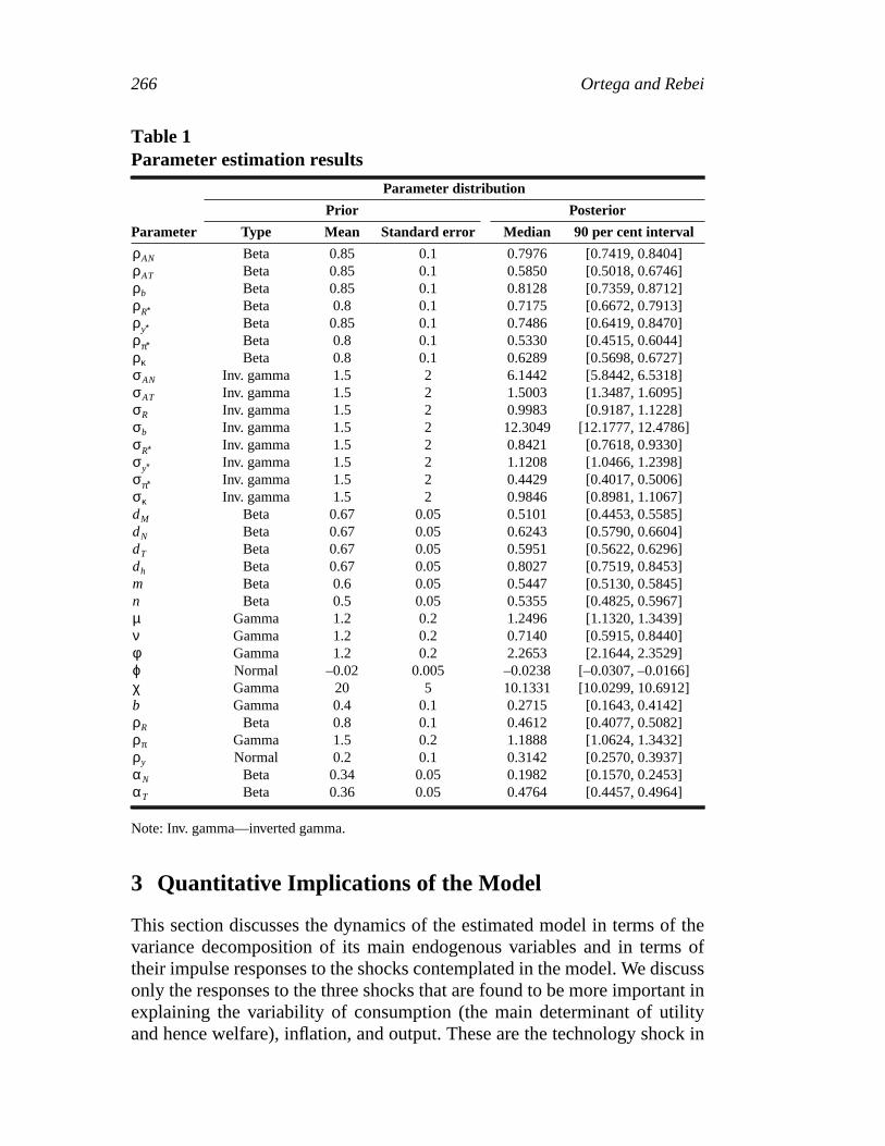
Table 1 shows the prior distributions imposed for the deep parameters of themodel, as well as the median and 90 per cent confidence interval for theposterior distributions.

It is important to note that all three sectors—domestic traded goods,imports, and non-traded goods—were given the same degree of nominalrigidity in the a priori distributions, in the form of an average priorprobability of not changing prices of 0.67, which corresponds to changingprices every three quarters, on average. But the prior of equal nominalrigidity across sectors did not hold, consistent with the findings of Bils andKlenow (2004), who document a high degree of heterogeneity in thefrequency of price changes across retail goods and services. Significantheterogeneity was found in the degree of price stickiness across sectors,since import prices were more flexible (with posterior median duration forprices of two quarters) and non-traded prices were stickier (posterior medianof almost three quarters). The prices of domestic traded goods wereestimated to have a posterior median duration of two and one-half quarters.Table 1 shows that the 90 per cent posterior confidence interval for doesnot even overlap with those for and . As with virtually any study thatexamines wage and price rigidities, the highest nominal stickiness is foundfor wages, with an estimated posterior duration of five quarters.

It is also worth noting that the posterior estimates of the Taylor rule almosthalve the prior degree of interest rate smoothing (posterior median

), somewhat reduce the reaction to deviations of inflation fromtarget to , and find a significant but low reaction to the outputgap, with a posterior median coefficient of . The historicalestimated Taylor rule, therefore, is an inflation-targeting rule with moderateconcern for output stabilization and with some sluggishness in the monetarypolicy instrument.

εRt εbtεκt

εANt εATdtεy* t επ* t εR* t

dMdN dT

ρR 0.46=ρπ 1.19=

ρy 0.3=


3 Quantitative Implications of the Model

This section discusses the dynamics of the estimated model in terms of thevariance decomposition of its main endogenous variables and in terms oftheir impulse responses to the shocks contemplated in the model. We discussonly the responses to the three shocks that are found to be more important inexplaining the variability of consumption (the main determinant of utilityand hence welfare), inflation, and output. These are the technology shock in

Table 1Parameter estimation results

Parameter distribution

Prior Posterior

Parameter Type Mean Standard error Median 90 per cent interval

Beta 0.85 0.1 0.7976 [0.7419, 0.8404]Beta 0.85 0.1 0.5850 [0.5018, 0.6746]Beta 0.85 0.1 0.8128 [0.7359, 0.8712]Beta 0.8 0.1 0.7175 [0.6672, 0.7913]Beta 0.85 0.1 0.7486 [0.6419, 0.8470]Beta 0.8 0.1 0.5330 [0.4515, 0.6044]Beta 0.8 0.1 0.6289 [0.5698, 0.6727]

Inv. gamma 1.5 2 6.1442 [5.8442, 6.5318]Inv. gamma 1.5 2 1.5003 [1.3487, 1.6095]Inv. gamma 1.5 2 0.9983 [0.9187, 1.1228]Inv. gamma 1.5 2 12.3049 [12.1777, 12.4786]Inv. gamma 1.5 2 0.8421 [0.7618, 0.9330]Inv. gamma 1.5 2 1.1208 [1.0466, 1.2398]Inv. gamma 1.5 2 0.4429 [0.4017, 0.5006]Inv. gamma 1.5 2 0.9846 [0.8981, 1.1067]

Beta 0.67 0.05 0.5101 [0.4453, 0.5585]Beta 0.67 0.05 0.6243 [0.5790, 0.6604]Beta 0.67 0.05 0.5951 [0.5622, 0.6296]Beta 0.67 0.05 0.8027 [0.7519, 0.8453]Beta 0.6 0.05 0.5447 [0.5130, 0.5845]Beta 0.5 0.05 0.5355 [0.4825, 0.5967]

Gamma 1.2 0.2 1.2496 [1.1320, 1.3439]Gamma 1.2 0.2 0.7140 [0.5915, 0.8440]Gamma 1.2 0.2 2.2653 [2.1644, 2.3529]Normal –0.02 0.005 –0.0238 [–0.0307, –0.0166]Gamma 20 5 10.1331 [10.0299, 10.6912]Gamma 0.4 0.1 0.2715 [0.1643, 0.4142]

Beta 0.8 0.1 0.4612 [0.4077, 0.5082]Gamma 1.5 0.2 1.1888 [1.0624, 1.3432]Normal 0.2 0.1 0.3142 [0.2570, 0.3937]

Beta 0.34 0.05 0.1982 [0.1570, 0.2453]Beta 0.36 0.05 0.4764 [0.4457, 0.4964]

Note: Inv. gamma—inverted gamma.

ρAN

ρAT

ρb

ρR∗ρy∗ρπ∗ρκσAN

σAT

σR

σb

σR∗σy∗σπ∗σκdM

dN

dT

dh

mnµνφϕχbρR

ρπρy

αN

αT


the non-traded-goods sector, the monetary policy shock, and the foreignmonetary policy shock.

3.1 Variance decomposition

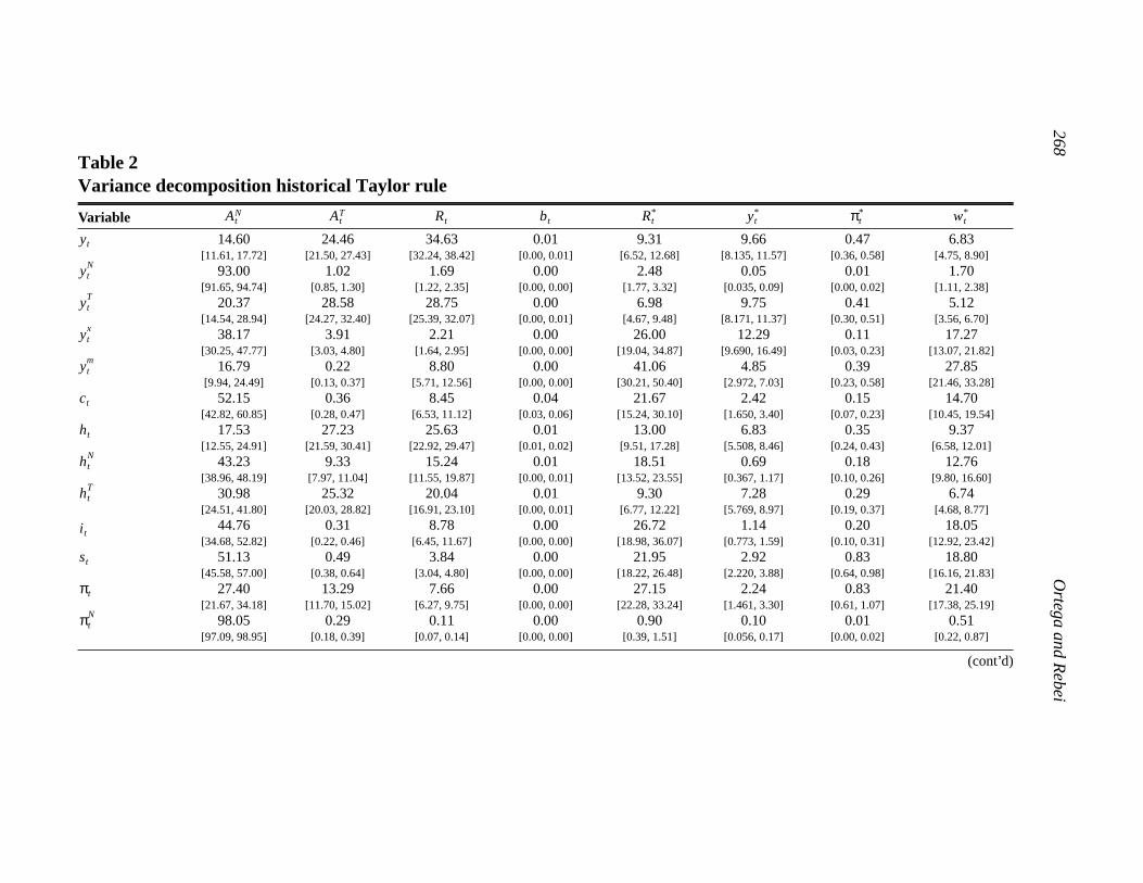
Table 2 shows the decomposition of the long-run variance of the mainendogenous variables of the model into the contribution of each of the eightshocks.

The business cycle volatility of the output in each production sector, tradedand non-traded, is explained mainly by its corresponding sector-specific tech-nology shock, but there is a substantial role for the monetary policy shocksas well, the domestic policy shocks on domestic traded production, andforeign shocks on exports and imports. Aggregate inflation is found to bebetter explained by technology shocks (through their impact on the non-traded inflation) and by foreign interest rate and risk-premium shocks(through the impact of both on imports inflation) than by monetary policyshocks in the past three decades. Final spending, i.e., consumption andinvestment, are explained mainly by the non-traded-goods technologyshock, which is one of the shocks with higher estimated volatility, althoughthe steady-state share of the non-traded-goods sector in final good is onlyone-third. Hours worked are substantially explained by technology shocks inthe two sectors, but are also clearly affected by monetary policy shocks.Finally, the volatility of the real exchange rate is explained by shocks totechnology, foreign monetary policy, and the risk premium.

3.2 Responses to a foreign shockunder the estimated monetary policy rule

The lines termed “historical” in Figure 2 represent the responses in terms ofpercentage deviations with respect to the steady state to a one-periodincrease of 100 basis points in the monetary policy instrument of the foreigneconomy, the United States.

The uncovered interest rate parity yields a nominal and real impact deprecia-tion of the Canadian dollar (2 per cent posterior median depreciation on theimpact of the real exchange rate, ). The real depreciation causes a directrise in the marginal cost of the importing firms and is therefore translatedinto higher import prices and fewer imports, . It is important to note,however, that as a result of the estimated sluggishness of import prices, theexchange rate pass-through is not complete and imports inflation rises byonly 50 basis points.

st

ytM

26

8O

rteg

a a

nd

Re

be

i

Table 2Variance decomposition historical Taylor rule

Variable

14.60 24.46 34.63 0.01 9.31 9.66 0.47 6.83[11.61, 17.72] [21.50, 27.43] [32.24, 38.42] [0.00, 0.01] [6.52, 12.68] [8.135, 11.57] [0.36, 0.58] [4.75, 8.90]

93.00 1.02 1.69 0.00 2.48 0.05 0.01 1.70[91.65, 94.74] [0.85, 1.30] [1.22, 2.35] [0.00, 0.00] [1.77, 3.32] [0.035, 0.09] [0.00, 0.02] [1.11, 2.38]

20.37 28.58 28.75 0.00 6.98 9.75 0.41 5.12[14.54, 28.94] [24.27, 32.40] [25.39, 32.07] [0.00, 0.01] [4.67, 9.48] [8.171, 11.37] [0.30, 0.51] [3.56, 6.70]

38.17 3.91 2.21 0.00 26.00 12.29 0.11 17.27[30.25, 47.77] [3.03, 4.80] [1.64, 2.95] [0.00, 0.00] [19.04, 34.87] [9.690, 16.49] [0.03, 0.23] [13.07, 21.82]

16.79 0.22 8.80 0.00 41.06 4.85 0.39 27.85[9.94, 24.49] [0.13, 0.37] [5.71, 12.56] [0.00, 0.00] [30.21, 50.40] [2.972, 7.03] [0.23, 0.58] [21.46, 33.28]

52.15 0.36 8.45 0.04 21.67 2.42 0.15 14.70[42.82, 60.85] [0.28, 0.47] [6.53, 11.12] [0.03, 0.06] [15.24, 30.10] [1.650, 3.40] [0.07, 0.23] [10.45, 19.54]

17.53 27.23 25.63 0.01 13.00 6.83 0.35 9.37[12.55, 24.91] [21.59, 30.41] [22.92, 29.47] [0.01, 0.02] [9.51, 17.28] [5.508, 8.46] [0.24, 0.43] [6.58, 12.01]

43.23 9.33 15.24 0.01 18.51 0.69 0.18 12.76[38.96, 48.19] [7.97, 11.04] [11.55, 19.87] [0.00, 0.01] [13.52, 23.55] [0.367, 1.17] [0.10, 0.26] [9.80, 16.60]

30.98 25.32 20.04 0.01 9.30 7.28 0.29 6.74[24.51, 41.80] [20.03, 28.82] [16.91, 23.10] [0.00, 0.01] [6.77, 12.22] [5.769, 8.97] [0.19, 0.37] [4.68, 8.77]

44.76 0.31 8.78 0.00 26.72 1.14 0.20 18.05[34.68, 52.82] [0.22, 0.46] [6.45, 11.67] [0.00, 0.00] [18.98, 36.07] [0.773, 1.59] [0.10, 0.31] [12.92, 23.42]

51.13 0.49 3.84 0.00 21.95 2.92 0.83 18.80[45.58, 57.00] [0.38, 0.64] [3.04, 4.80] [0.00, 0.00] [18.22, 26.48] [2.220, 3.88] [0.64, 0.98] [16.16, 21.83]

27.40 13.29 7.66 0.00 27.15 2.24 0.83 21.40[21.67, 34.18] [11.70, 15.02] [6.27, 9.75] [0.00, 0.00] [22.28, 33.24] [1.461, 3.30] [0.61, 1.07] [17.38, 25.19]

98.05 0.29 0.11 0.00 0.90 0.10 0.01 0.51[97.09, 98.95] [0.18, 0.39] [0.07, 0.14] [0.00, 0.00] [0.39, 1.51] [0.056, 0.17] [0.00, 0.02] [0.22, 0.87]

(cont’d)

AtN At

T Rt bt Rt* yt

* πt* wt

*

yt

ytN

ytT

ytx

ytm

ct

ht

htN

htT

i t

st

πt

πtN

Th

e W

elfa

re Im

plica

tion

s of In

flatio

n ve

rsus P

rice-L

eve

l Ta

rge

ting

26

9

Table 2 (cont’d)Variance decomposition historical Taylor rule

Variable14.49 60.50 4.94 0.00 11.07 2.00 0.19 6.78

[11.75, 17.36] [55.31, 67.17] [4.11, 6.31] [0.00, 0.00] [6.40, 16.60] [1.339, 2.77] [0.11, 0.25] [4.20, 9.49]

19.34 3.90 6.05 0.00 36.23 3.33 1.25 29.86[15.02, 23.34] [3.17, 4.54] [4.77, 7.70] [0.00, 0.00] [30.88, 41.38] [2.429, 4.63] [1.00, 1.52] [26.00, 33.51]

13.12 11.57 0.94 0.00 31.57 4.58 12.86 25.32[10.23, 16.58] [9.58, 13.94] [0.73, 1.23] [0.00, 0.00] [26.33, 37.17] [3.503, 5.94] [11.14, 14.45] [22.18, 28.69]

26.18 3.25 27.18 0.00 24.52 0.25 0.39 18.20[21.26, 30.10] [2.82, 3.75] [21.58, 34.16] [0.00, 0.00] [17.75, 32.11] [0.126, 0.46] [0.24, 0.54] [13.32, 22.76]

AtN At

T Rt bt Rt* yt

* πt* wt

*

πtTd

πtm

πtx

Rt


Exports benefit from the depreciation. Because exports are priced in theforeign currency, but traded-sector firms maximize their profits in Canadiandollars, the depreciation by itself increases the benefits from the portion ofthe production that is exported. As a result, producers in the traded-goodssector lower export prices and increase their exports on impact.

The increase of imports inflation makes aggregate inflation rise, whichcauses a monetary policy contraction. That, in turn, decreases demand (and ) that further reduces imports demand but also decreases demand ofnon-traded and of traded goods produced domestically. The monetary policycontraction also helps undo the initial depreciation.

3.3 Responses to a sectoral shockunder the estimated monetary policy rule

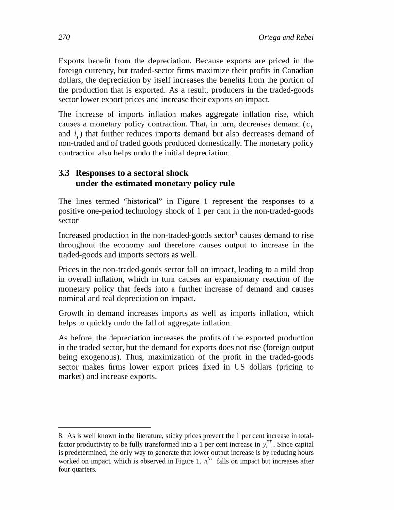
The lines termed “historical” in Figure 1 represent the responses to apositive one-period technology shock of 1 per cent in the non-traded-goodssector.

Increased production in the non-traded-goods sector8 causes demand to risethroughout the economy and therefore causes output to increase in thetraded-goods and imports sectors as well.

Prices in the non-traded-goods sector fall on impact, leading to a mild dropin overall inflation, which in turn causes an expansionary reaction of themonetary policy that feeds into a further increase of demand and causesnominal and real depreciation on impact.

Growth in demand increases imports as well as imports inflation, whichhelps to quickly undo the fall of aggregate inflation.

As before, the depreciation increases the profits of the exported productionin the traded sector, but the demand for exports does not rise (foreign outputbeing exogenous). Thus, maximization of the profit in the traded-goodssector makes firms lower export prices fixed in US dollars (pricing tomarket) and increase exports.

8. As is well known in the literature, sticky prices prevent the 1 per cent increase in total-factor productivity to be fully transformed into a 1 per cent increase in . Since capitalis predetermined, the only way to generate that lower output increase is by reducing hoursworked on impact, which is observed in Figure 1. falls on impact but increases afterfour quarters.

cti t

ytNT

htNT


3.4 Responses to a common domestic shockunder the estimated monetary policy rule

The lines termed “historical” in Figure 3 represent the responses to a tempo-rary monetary policy contraction. The nominal interest rate shock increasesby 100 basis points for one period. On impact, the monetary policy instru-ment rises by less than 1 per cent because of the immediate fall in inflationand because of the presence of significant interest rate smoothing. In fact,nominal interest rates rise by only one-half of the 1 per cent shock. Inflationfalls on impact owing to an immediate decrease in demand and consequentlyin activity in every sector—traded goods, non-traded goods, and imports.

The monetary policy contraction causes a nominal and real impact appreci-ation of the Canadian dollar. Since export prices are being set in US dollars,the appreciation reduces exporters’ profits and export prices consequentlyrise, which causes a drop in exports.

4 Simple Inflation-Targeting Rules

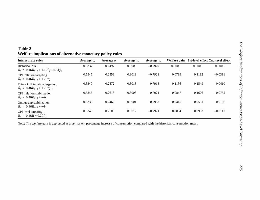
In this section, we search for the parameterization of feedback Taylor-typeinterest rate rules, similar to equation (30), that maximize household welfaregiven our estimated model. We evaluate the welfare gain they represent withrespect to the estimated monetary policy reaction function (or “historicalrule” in the tables), as well as their implications in terms of aggregatefluctuations.

The welfare implications are shown in Table 3. Table 4 reports anotherdimension for comparing alternative monetary policy reaction functions: theunconditional volatility they imply for the utility and its arguments, as wellas for several crucial macro variables, i.e., output, inflation, and the nominalinterest rate. We also compute the long-run variance decomposition (Table5) and the impulse responses to different shocks (in Figures 1, 2, and 3) forvarious monetary policy rule specifications.

The search for the welfare-maximizing feedback monetary policy rules is setout as follows. We maximize the unconditional expectation of lifetime


Figure 1Non-tradables technology shock

0.3

0.2

0.1

0.0

–0.1

Zt

0 5 10 15 20

0.20

0.15

0.10

0.05

–0.05

YN,t

0 5 10 15 20

0.15

0.10

0.05

0.00

–0.05

YT,t

0 5 10 15 20

0.00

0.10

0.05

0.00

–0.05

–0.15

Rt

0 5 10 15 20

–0.10

0.05

0.00

–0.05

–0.10

–0.15

pti

0 5 10 15 20

0.4

0.3

0.2

0.1

wt

0 5 10 15 200.0

0.5

0.0

–0.5

–1.0

πN,t

0 5 10 15 20

0.10

0.05

0.00

–0.05

–0.15

πT,t

0 5 10 15 20

–0.10

Flexible prices Historical Optimal


Figure 2Foreign nominal interest rate shock

0.5

0.0

–0.5

–1.0

–1.5

Zt

0 5 10 15 20

0.2

0.1

0.0

–0.1

–0.3

YN,t

0 5 10 15 20

1.0

0.5

0.0

–0.5

YT,t

0 5 10 15 20

–0.2

0.8

0.6

0.4

0.2

–0.2

Rt

0 5 10 15 20

0.0

0.6

0.4

0.2

0.0

–0.2

pti

0 5 10 15 20

0.5

0.0

–0.5

–1.0

wt

0 5 10 15 20

–1.5

1.0

0.5

–0.5

–0.1

πN,t

0 5 10 15 20

1.0

0.5

0.0

–0.5

πT,t

0 5 10 15 20

–1.0

–2.0

–2.0

0.0



Figure 3Local nominal interest rate shock

0.5

0.0

–0.5

–1.0

–1.5

Zt

0 5 10 15 20

0.1

0.0

–0.1

–0.2

–0.4

YN,t

0 5 10 15 20

0.0

–0.2

–0.4

–0.6

–0.8

YT,t

0 5 10 15 20

–0.3

1.0

0.5

0.0

–0.5

Rt

0 5 10 15 20–1.0

0.5

0.0

–0.5

–1.0

pti

0 5 10 15 20

0.4

0.3

0.2

0.1

wt

0 5 10 15 20

0.0

0.5

0.0

–0.5

–0.1

πN,t

0 5 10 15 20

0.5

0.0

–0.5

–1.0

πT,t

0 5 10 15 20

–0.1


Th

e W

elfa

re Im

plica

tion

s of In

flatio

n ve

rsus P

rice-L

eve

l Ta

rge

ting

27

5

Table 3Welfare implications of alternative monetary policy rules

Interest rate rules Average Average Average Average Welfare gain 1st-level effect 2nd-level effect

Historical rule 0.5337 0.2497 0.3005 –0.7929 0.0000 0.0000 0.0000

CPI inflation targeting 0.5345 0.2558 0.3013 –0.7921 0.0799 0.1112 –0.0311

Future CPI inflation targeting 0.5349 0.2572 0.3018 –0.7918 0.1136 0.1549 –0.0410

CPI inflation stabilization 0.5345 0.2618 0.3008 –0.7921 0.0847 0.1606 –0.0755

Output-gap stabilization 0.5333 0.2462 0.3001 –0.7933 –0.0415 –0.0551 0.0136

CPI level targeting 0.5345 0.2500 0.3012 –0.7921 0.0834 0.0952 –0.0117

Note: The welfare gain is expressed as a permanent percentage increase of consumption compared with the historical consumption mean.

ct mt ht ut

Rt 0.46Rt 1– 1.19πt 0.31yt+ +=

Rt 0.46Rt 1– 1.20πt+=

Rt 0.46Rt 1– 1.20πt 1++=

Rt 0.46Rt 1– ∞πt+=

Rt 0.46Rt 1– ∞ yt+=

Rt 0.46R 0.20Pt+=


utility9 of households over the parameters of the Taylor rule. This implies:

.

We measure the welfare gain associated with a particular monetary policy interms of its compensating variation. That is, we calculate the percentage oflifetime consumption that should be added to that obtained under theestimated Taylor rule in order to give households the same unconditionalexpected utility as under the scenario for the new monetary policy rule:

,

where variables without tildes are obtained under the estimated ruledescribed before, and variables with tildes are under the optimized Taylorrule. Based on the results found in Kim and Kim (2003) and subsequentliterature, we compute the long-run average utility by means of a second-order approximation around the steady-state utility. In particular, we followthe approach of Schmitt-Grohé and Uribe (2004a).

,

where and are the first and second derivatives, respectively, of theutility function with respect to its arguments, evaluated at their deterministicsteady-state values; variables with hats measure deviations from their levelsin the deterministic steady state. The compensating variation in consump-tion can therefore be decomposed into a first-level effect and a second-levelor stabilization effect, i.e., into the welfare gains of the new parameterizationof the monetary policy owing to the effect of monetary policy on the averagelevels of consumption, real balances, and leisure, as well as its effect on theirvolatilities. The first-level effect is defined as:

9. Schmitt-Grohé and Uribe (2004b) adopt the conditional welfare optimization in theirframework and they consider the non-stochastic steady state as an initial state of theeconomy. By computing the unconditional long-run utility, we do not consider the effect ofthe initial state. Transition costs are crucially dependent on that initial state, especially ifthe real state of the economy is never at the deterministic level. In addition, Schmitt-Grohéand Uribe show that the optimal rule is robust to these definitions of welfare, but that thewelfare improvement could be different in the sense that it is higher in the case ofunconditional welfare given that no short-term transition costs are incurred.

maxρπ ρy,

E u ct mt ht, ,( ){ }

E u ct 1 welfare gain+( ) mt ht, ,( ){ } E u ct mt ht, ,( ){ }=

E u ct mt ht, ,( )( ) u c m h, ,( ) u′E ctˆ mt

ˆ htˆ, ,( )+=

12---E ct

ˆ mtˆ ht

ˆ, ,( )′u″ ctˆ mt

ˆ htˆ, ,( )+

u ′ u″


,

and the second-level effect as:

.

The overall effect in all cases is such that, approximately,. Table 3 reports the welfare

gains, together with the unconditional long-run average values of thearguments of the utility function as well as that of the log utility itself.

In what follows, we limit our attention to the Taylor-type rules thatguarantee the existence of a unique and stable equilibrium in theneighbourhood of the deterministic steady state. We also restrict our searchto monetary policy reactions to price and output deviations from target; wedo this by keeping the degree of nominal interest rate smoothing unchangedand equal to the posterior median of the estimated value, i.e., .10

Our reference interest rate feedback rule is the estimated one where, on topof the moderate nominal interest rate smoothing, the monetary authority hastargeted inflation but not very aggressively (the posterior median estimatefor the reaction to deviations of the aggregate CPI inflation from target is

10. Several reasons motivate the choice of fixing . One is that without interest ratesmoothing there would be indeterminacy for values of the coefficient on inflation smallerthan one. By keeping at its estimated value, we can compute the welfare gains of a widerrange of values for , including those smaller than one.

Another important reason is that because the optimized rule would aim at maximizinginflation stabilization rather than instrument smoothing, the welfare-maximizing value of

is very likely going to be zero. Indeed, Schmitt-Grohé and Uribe (2004b) find that theoptimal degree of interest rate smoothing for Taylor rules in the Christiano, Eichenbaum,and Evans (2001) model is zero. However, they also look for, as we do, the parameterizationof the Taylor rule that delivers higher utility for degrees of interest rate smoothing closer tothe observed ones. Keeping our frame of analysis of alternative monetary policy reactionfunctions close to the observed features of monetary policy as it is implemented in practiceconstitutes a further reason for keeping fixed as well as for remaining with simple Taylorrules. A final reason is that maximizing welfare over several parameters is computationallyexpensive.

E u ct 1 1st-level effect+( ) mt ht, ,( ){ } u c m h, ,( )=

u′E ctˆ mt

ˆ htˆ, ,( )+

E u ct 1 2nd-level effect+( ) mt ht, ,( ){ } u c m h, ,( )=

12---E ct

ˆ mtˆ ht

ˆ, ,( )′+

u″ ctˆ mt

ˆ htˆ, ,( )

1 welfare gain+( )1 1st-level effect+( ) 1 2nd-level effect+( )≈

ρR 0.46=

ρR

ρR

ρπ

ρR

ρR


slightly above 1, ) and there has been a significant though weakresponse of the monetary policy to the output gap (posterior median of

).

4.1 CPI inflation-rate targeting

Here we consider the case where the central bank targets the same variablesas in the historical rule, i.e., aggregate CPI inflation and the output gap.The welfare-maximizing Taylor rule implies a very similar level ofaggressiveness with respect to inflation deviations from target to that of theestimated historical rule, , but, unlike the historical case, there isno response to the output gap, .

The historical rule entails a welfare cost of 0.08 per cent of the lifetimeconsumption associated with the optimized CPI inflation-targeting rule (seesecond row in Table 3). Most of the welfare improvement of choosing

and rather than the estimated parameters comes fromthe first-level effect or improvement in long-run average utility, whichamounts to a 0.11 per cent increase in lifetime consumption. This welfare-maximizing monetary policy reaction function implies slightly highervolatility in the utility arguments (see second row of Table 4), which iscaptured by a negative second-order effect, as well as in output, while it onlymarginally improves inflation stabilization.

As Table 4 shows, not only consumption and the other arguments in theutility function show higher volatility; so do output and the monetary policyinstrument. Instead, inflation remains with similar levels of volatility.Table 5 shows the medians of the long-run variance decomposition of modelvariables under this new monetary policy rule. It does not differ much fromthat in Table 2. However, it is worth noting that consumption variability isbetter explained by domestic shocks, including the monetary policy shock,and less by foreign shocks than under the historical rule. Inflation variabilityowes much more to monetary policy shocks than under the historical rule,but the explanatory power of foreign shocks has not substantially decreased.In general, monetary policy shocks are more responsible for aggregatevariability under this optimized strict inflation-targeting rule than under thehistorical one.

In terms of the responses to shocks, the impulse responses obtainedreplacing the historical rule with this new optimized CPI inflation-targetingrule are quite similar. The median responses are displayed in Figures 1 to 3

ρπ 1.19=

ρy 0.31=

ρπ 1.20=ρy 0=

ρπ 1.20= ρy 0=

Th

e W

elfa

re Im

plica

tion

s of In

flatio

n ve

rsus P

rice-L

eve

l Ta

rge

ting

27

9

Table 4Aggregate volatility induced by alternative monetary policy regimes

Interest rate rules

Historical rule 0.0133 0.0552 0.0112 0.0226 0.0173 0.0077 0.0098

CPI inflation targeting 0.0163 0.0596 0.0128 0.0301 0.0301 0.0076 0.0126

Future CPI inflation targeting 0.0158 0.0595 0.0205 0.0277 0.0440 0.0140 0.0128

CPI inflation stabilization 0.0212 0.0624 0.0114 0.0357 0.0345 0.0007 0.0137

Output-gap stabilization 0.0120 0.0525 0.0115 0.0245 0.0097 0.0084 0.0077

CPI level targeting 0.0150 0.0564 0.0102 0.0276 0.0268 0.0065 0.0108

Note: denotes the unconditional standard deviation for the listed variables.

σc σm σh σu σy σπ σR

Rt 0.46Rt 1– 1.19πt 0.31yt+ +=

Rt 0.46Rt 1– 1.20πt+=

Rt 0.46Rt 1– 1.20πt 1++=

Rt 0.46Rt 1– ∞πt+=

Rt 0.46Rt 1– ∞ yt+=

Rt 0.46Rt 1– 0.20Pt+=

σ


(under optimal inflation-targeting rule), together with those that would havebeen obtained in the case of flexible prices and wages.11

5 Price-Level Targeting

As stated in the introduction, many issues arise when a price-level target isintroduced, such as the implications for the price level and responses ofinflation to shocks, as well as for the volatility of the main macro variables,not the least of which is inflation itself.

Starting with Wicksell (1907), numerous authors have considered aggregateprice-level stability the main goal of central banks, and this is reflected inthe mandates of many central banks. How to achieve price stability has moreoften been interpreted as targeting at an explicit inflation rate or range thanat a specific price-level path. Still, some recent research has shown that therecan be substantial gains in including a specific price-level target in themonetary policy reaction function. In the above-mentioned Bank of Canada(1998) publication, Coulombe (1998) shows that there is a clear information

11. However, we keep the rest of the estimated parameters of Table 1, including thosereferring to the monetary policy reaction function. Suppressing the latter would mean notbeing able to solve the model.

Table 5Variance decomposition, optimized CPI inflation-targeting rule

Variable

15.19 33.73 31.40 0.01 7.05 6.97 0.50 5.14

90.56 0.17 3.71 0.00 3.17 0.25 0.05 2.08

10.27 40.69 30.68 0.01 5.91 7.56 0.50 4.37

37.49 9.77 9.25 0.01 19.77 10.94 0.25 12.53

22.12 1.07 12.86 0.01 36.44 3.36 0.71 23.44

54.83 1.29 11.91 0.03 18.02 1.93 0.30 11.69

15.50 6.23 40.48 0.03 16.60 8.82 0.69 11.64

32.52 0.79 27.97 0.02 21.57 2.41 0.42 14.29

26.46 8.23 34.15 0.02 12.59 9.03 0.61 8.92

48.94 1.74 13.23 0.00 21.06 1.19 0.39 13.45

57.85 0.64 9.06 0.00 16.19 0.65 0.71 14.89

22.25 2.48 25.56 0.00 26.44 0.12 0.71 22.44

97.76 0.06 0.60 0.00 0.93 0.05 0.01 0.58

15.97 45.91 13.56 0.00 13.09 2.67 0.28 8.52

29.52 0.35 16.47 0.00 27.75 0.24 1.03 24.64

16.25 18.61 2.87 0.00 25.16 1.87 14.65 20.60

29.29 1.93 22.15 0.00 26.02 0.18 0.55 19.89

AtN At

T Rt bt Rt* yt

* πt* wt

yt

ytN

ytT

ytx

ytm

ct

ht

htN

htT

i t

st

πt

πtN

πtTd

πtm

πtx

Rt


gain under an explicit price-level-targeting regime: the price level itselfconveys useful information about future inflation, because past shocks toprices must be reversed in the future. Under strict inflation targeting,however, where all shocks to the price level are permanent, the price levelreveals no useful information. In Bank of Canada (1998), Black, Macklem,and Rose (1998) show that, when comparing simple monetary policy rulesin a calibrated small open economy one-good model of the Canadianeconomy, and provided the price-level target is credible and that privatesector expectations of inflation adjust accordingly, the economy performsbetter with a price-level target than with an inflation target, in the sense thatthe variability of both inflation and output are lower with the price-leveltarget. These potential benefits of price-level targeting are not without risks,however. How to communicate such policy is a challenge. It could bedifficult to justify why, following an increase in inflation above its long-runaverage, inflation had to be reduced below this long-run average for sometime to drive the price level back to its target. Also, that reduction ininflation after the monetary policy takes action can lead to sharper initialdeclines in economic activity than under a strict inflation-targeting regime.

Giannoni (2000) argues that simple price-level-targeting rules,12 while assimple as standard inflation-targeting Taylor rules, have received consider-ably less attention in recent studies of monetary policy. It is widely believedthat such rules would result in greater variability of inflation (and, undernominal rigidity, of the output gap), since the policy-maker would respondto an inflationary shock by generating a deflation in subsequent periods.Studies such as Lebow, Roberts, and Stockton (1992) and Haldane andSalmon (1995) support this conventional view. However, Giannoni showsthat when agents are forward looking and the monetary authority crediblycommits to a price-level-targeting rule, such a Wicksellian rule yields lowervariability of inflation and of nominal interest rates. Agents’ expectation of afuture deflation after an inflationary shock dampens the initial increase ininflation, lowers the variability of inflation, and causes welfare to rise.Williams (1999) confirms this result using the FRB/US model.

More recently, and closer to our approach, Batini and Yates (2003) alsochallenge the established view that price-level targeting entails lower price-level variance at the expense of higher inflation and output variance. Theyinvestigate monetary policy regimes that combine price-level and inflation

12. In those rules, the nominal interest rate deviates from a constant in response to theoutput gap and to deviations of the price level from a prespecified path of constant inflation.Giannoni (2000) follows Woodford (1998, 2003) in referring to such rules as “Wick-sellian.” Wicksell (1907) argued that “price stability” could be obtained by allowing theinterest rate to respond positively to fluctuations in the price level.


targeting in a variety of models and conclude that the relative merits of eachregime depend on several modelling and policy assumptions, and do so in anon-monotonic fashion when moving from one regime to another.

In this section, we conduct the same calculations of welfare gains andimplied macroeconomic volatility as before, but we consider a different typeof monetary policy reaction function, i.e., where the central bank isconcerned with returning the price level to its target path as well as orinstead of bringing inflation to target.13

We follow Batini and Yates (2003) and encompass price-level and inflationtargeting using the following specification of the monetary policy reactionfunction:

,

where is the target or steady-state value for the price level at period ,compatible with the established inflation target. Note that for , wehave exactly the case of the Taylor rule defined for the inflation rate, while

means pure price-level targeting. For , the rule is ahybrid one where the central bank is concerned about reaching the inflationtarget rate but also about the evolution of prices on the way to the inflationtarget. As before, we keep and fixed while jointlyoptimizing over and over .

Figure 4 shows the utility surface of this optimization exercise, while furtherwelfare implications and the implied volatility are shown in the last row ofTables 3 and 4. Two results emerge from this exercise. First, it is almostimpossible to establish a clear ranking of combinations of parameters in thiscase; the long-run utility level (the vertical axis in Figure 4) associated withthe depicted parameter surface is virtually the same. Pure approximationerrors embedded in our procedure could be behind the plotted differences.Second, for the central bank to give a non-zero weight to the deviations ofthe price level from its target path, i.e., for , the monetary policyreaction to price and inflation deviations from target has to be very low,

. In that case, welfare is maximized for the hybrid rule with, i.e., where 25 per cent of the price-stability concern of the

monetary authority takes the form of inflation targeting and the rest is pure

13. We have computed the simulated impulse responses of the main macro variables afterall shocks in the economy and find very similar reactions under pure inflation targeting asunder pure price-level targeting for the same degree of price stabilization (samecoefficient).

ρP

Rt R⁄( )log ρR Rt 1– R⁄( ) ρP Pt Pt⁄( )log[+log=

ηP Pt 1– Pt 1–⁄( ) ]log– ρy yt y⁄( )log+

Pt tηP 1=

ηP 0= 0 ηP 1< <

ρR 0.46= ρy 0=0 ηP 1≤ ≤ ρP

ηP 1<

ρP 0.2=ηP 0.25=


Figure 4Inflation versus price-level targeting

–0.7920

–0.7920

–0.7921

–0.7921

–0.7921

–0.7921

–0.7921

–0.7922

–0.7922

3.02.5

2.01.5

1.00.5

0.0

Util

ity

1.0

0.8

0.6

0.4

0.2

0.0

ηP

ρP


price-level targeting. Still, the welfare gain is almost unnoticeable andcomes from the lower volatility induced (smaller negative second-leveleffect) by the mild reaction of the monetary policy.

It is interesting that gains from an explicit price-level target come only withlow policy reactions, causing a far longer time to bring about price andinflation stabilization than in strict inflation-targeting regimes. This result isin line with the findings of Smets (2003).

6 Targeting Future Price Developments

To conclude these optimization exercises for simple monetary policy rules,we explore the impact of targeting expected future deviations of the inflationrate or the price level rather than targeting contemporaneous deviations. Intheir analysis of price-level versus inflation targeting under different modelspecifications, policy rules, and loss functions of the central bank, Batini andYates (2003) find that the more forward looking the model, the less notice-able the difference between the reaction functions of inflation and price-level targeting.

We find two main results: (i) the welfare-maximizing parameter set is thesame as when the central bank is not forward looking, i.e., ,

, and ; and (ii) the welfare attained with a forward-looking monetary policy rule is noticeably higher. Row 3 of Table 3 showsthat the welfare gain now is 0.11 per cent of the lifetime consumption versus0.08 per cent when optimizing a contemporary monetary policy rule. Andthis welfare gain comes with increased output and inflation volatility butwith lower volatility in household utility (see row 3 in Table 4).

Of all of the possible specifications explored in this paper, the one thatachieves a higher welfare given the estimated model for the Canadianeconomy without causing substantial excess macroeconomic volatility is astrict inflation-targeting rule where the central bank reacts to the nextperiod’s expected deviation from the inflation target and does not target theoutput gap but allows for a moderate degree of nominal interest ratesmoothing.

Conclusion

We analyze welfare-improving monetary policy reaction functions in thecontext of a New Keynesian small open economy model with a traded-goodssector and a non-traded-goods sector and with sticky prices and wages. Weestimate the model for the case of Canada and use it to evaluate the welfaregains of alternative specifications of the feedback nominal interest rate rule.

ρπ+1 1.2=

ρπ+1w 0= ρπ

+1 0=


The model is estimated using Bayesian techniques for quarterly Canadiandata. We find statistically significant heterogeneity in the degree of pricerigidity across sectors. We explore what would have been the optimalparameterization of a Taylor rule such as the estimated one, where thecentral bank targets aggregate inflation. We find welfare gains in respondingslightly more aggressively to aggregate inflation deviations from target thanhas been the case in the past three decades, and in not responding to theoutput gap, as opposed to what the Bank of Canada has done.

We then consider recent literature that has questioned the optimality ofaiming at a stable inflation rate instead of a stable price level in a worldwhere households would prefer to reduce uncertainty about the long-runpurchasing value of money. We look for the welfare-maximizing specifica-tion of an interest rate reaction function that targets a combination of price-level and inflation targets or just one of the two. We find no clear welfaregain in moving towards price-level targeting, unless the monetary policy iswilling to accept very long horizons for prices and inflation to get back totarget.

We find that higher welfare, without inducing excess macroeconomic volati-lity, is achieved with a strict inflation-targeting rule, where the central bankreacts to next period’s expected deviation from the inflation target and doesnot target the output gap but allows for a moderate degree of nominalinterest rate smoothing.

References

Ambler, S., A. Dib, and N. Rebei. 2003. “Nominal Rigidities and ExchangeRate Pass-Through in a Structural Model of a Small Open Economy.”Bank of Canada Working Paper No. 2003–29.

Bailliu, J. and H. Bouakez. 2004. “Exchange Rate Pass-Through inIndustrialized Countries.”Bank of Canada Review (Spring): 19–28.

Bank of Canada. 1998.Price Stability, Inflation Targets, and MonetaryPolicy. Proceedings of a conference held by the Bank of Canada, May1997. Ottawa: Bank of Canada.

Batini, N. and A. Yates. 2003. “Hybrid Inflation and Price-Level Targeting.”Journal of Money, Credit and Banking 35 (3): 283–300.

Bergin, P.R. 2003. “Putting the ‘New Open Economy Macroeconomics’ to aTest.”Journal of International Economics 60 (1): 3–34.

Bils, M. and P.J. Klenow. 2004. “Some Evidence on the Importance of StickyPrices.”Journal of Political Economy 112 (5): 947–85.


Black, R., T. Macklem, and D. Rose. 1998. “On Policy Rules for PriceStability.” In Price Stability, Inflation Targets, and Monetary Policy,41–61. Proceedings of a conference held by the Bank of Canada,May 1997. Ottawa: Bank of Canada.

Calvo, G.A. 1983. “Staggered Prices in a Utility-Maximizing Framework.”Journal of Monetary Economics 12 (3): 383–98.

Campa, J.M. and L.S. Goldberg. 2002. “Exchange Rate Pass-Through intoImport Prices: A Macro and Micro Phenomenon?” National Bureau ofEconomic Research Working Paper No. 8934.

Christiano, L.J., M. Eichenbaum, and C.L. Evans. 2001. “Nominal Rigiditiesand the Dynamic Effects of a Shock to Monetary Policy.” National Bureauof Economic Research Working Paper No. 8403.

———. 2005. “Nominal Rigidities and the Dynamic Effects of a Shock toMonetary Policy.”Journal of Political Economy 113 (1): 1–45.

Coulombe, S. 1998. “The Intertemporal Nature of Information Conveyed bythe Price System.” InPrice Stability, Inflation Targets, and MonetaryPolicy, 3–28. Proceedings of a conference held by the Bank of Canada,May 1997. Ottawa: Bank of Canada.

ECU Institute. 1995.International Currency Competition and the FutureRole of the Single European Currency. London: Kluwer LawInternational.

Engel, C. and J.H. Rogers. 1996. “How Wide Is the Border?”AmericanEconomic Review 86 (5) 1112–125.

Ghosh, A. and H. Wolf. 2001. “Imperfect Exchange Rate Passthrough:Strategic Pricing and Menu Costs.” CESifo Working Paper No. 436.

Giannoni, M. 2000. “Optimal Interest-Rate Rules in a Forward-LookingModel, and Inflation Stabilization versus Price-Level Stabilization.”Federal Reserve Bank of New York. Photocopy.

Haldane, A.G. and C.K. Salmon. 1995. “Three Issues on Inflation Targets.”In Targeting Inflation, edited by A.G. Haldane, 170–98. Bank of England.

Kichian, M. 2001. “On the Nature and the Stability of the Canadian PhillipsCurve.” Bank of Canada Working Paper No. 2001–4.

Kim, J. and S.H. Kim. 2003. “Spurious Welfare Reversals in InternationalBusiness Cycle Models.”Journal of International Economics 60 (2):471–500.

Kollmann, R. 2002. “Monetary Policy Rules in the Open Economy: Effectson Welfare and Business Cycles.”Journal of Monetary Economics49 (5):989–1015.

Lane, P.R. 2001. “The New Open Economy Macroeconomics: A Survey.”Journal of International Economics 54 (2): 235–66.


Lebow, D.E., J.M. Roberts, and D.J. Stockton. 1992. “EconomicPerformance under Price Stability.” Federal Reserve Board, Division ofResearch and Statistics, Working Paper No. 125.

Leung, D. 2003. “An Empirical Analysis of Exchange Rate Pass Throughinto Consumer Prices.” Bank of Canada RM–03–005.

Obstfeld, M. and K. Rogoff. 1995. “Exchange Rate Dynamics Redux.”Journal of Political Economy 103 (3): 624–60.

Ortega, E. and N. Rebei. 2005. “A Two Sector Small Open Economy Model:Which Inflation to Target.” Bank of Canada. Photocopy.

Schmitt-Grohé, S. and M. Uribe. 2004a. “Solving Dynamic GeneralEquilibrium Models Using a Second-Order Approximation to the PolicyFunction.”Journal of Economic Dynamics and Control 28 (4): 755–75.

———. 2004b. “Optimal Operational Monetary Policy in the Christiano-Eichenbaum-Evans Model of the U.S. Business Cycle.” National Bureauof Economic Research Working Paper No. 10724.

Smets, F. 2003. “Maintaining Price Stability: How Long Is the MediumTerm?”Journal of Monetary Economics 50 (6): 1293–309.

Smets, F. and R. Wouters. 2002. “Openness, Imperfect Exchange RatePass-Through and Monetary Policy.”Journal of Monetary Economics49 (5): 947–81.

———. 2003. “An Estimated Dynamic Stochastic General EquilibriumModel of the Euro Area.”Journal of the European Economic Association1 (5): 1123–175.

Wicksell, K. 1907. “The Influence of the Rate of Interest on Prices.”Economic Journal 17 (66): 213–20.

Williams, J.C. 1999. “Simple Rules for Monetary Policy.” Federal ReserveBoard, Finance and Economics Discussion Series Paper No. 1999–12.

Woodford, M. 1998. “Doing without Money: Controlling Inflation in a Post-Monetary World.”Review of Economic Dynamics 1 (1): 173–219.

———. 2003.Interest and Prices: Foundations of a Theory of MonetaryPolicy. Princeton: Princeton University Press.

Documents

The Welfare Implications of Inﬂation versus Price-Level ... · 254 Ortega and Rebei In this paper, we have two main objectives. First, we want to characterize the simple, Taylor-type