11-222

Research Group: Finance in Toulouse February, 2011

The WACC Fallacy: The Real Effects of Using a Unique Discount Rate

PHILIPP KRUGER, AUGUSTIN LANDIER AND DAVID THESMAR

Electronic copy available at: http://ssrn.com/abstract=1764024

The WACC Fallacy: The Real Effects of

Using a Unique Discount Rate 1

Philipp KrugerGeneva Finance Research Institute - Universite de Geneve

Augustin LandierToulouse School of Economics

David ThesmarHEC Paris and CEPR

February 2011

Abstract

We document investment distortions induced by the use of a singlediscount rate within firms. According to textbook capital budgeting,firms should value any project using a discount rate determined by therisk characteristics of the project. If they use a unique company-widediscount rate, they overinvest (resp. underinvest) in divisions with amarket beta higher (resp. lower) than the firm’s core industry beta.We directly test this consequence of the “WACC fallacy”and establisha robust and significant positive relationship between division-level in-vestment and the spread between the division’s market beta and thefirm’s core industry beta. Consistently with bounded rationality the-ories, this bias is stronger when the measured cost of taking the wrongdiscount rate is low, for instance, when the division is small. Finally,we measure the value loss due to the WACC fallacy in the contextof acquisitions. Bidder abnormal returns are higher in diversifyingmergers and acquisitions in which the bidder’s beta exceeds that ofthe target. On average, the present value loss is about 0.7% of thebidder’s market equity.

JEL-Classification: G11, G31, G34Keywords: Investment, Behavioral finance, Cost of capital

1Corresponding Author: Philipp Kruger. Email: philipp.krueger@unige.ch, Telephone:+41 (0)22 379 85 69. Augustin Landier, augustin.landier@tse-fr.eu, Telephone: +33 (0)561 12 86 88. David Thesmar, thesmar@hec.fr, Telephone: +33 (0)1 39 67 94 12. We thankBoris Vallee for excellent research assistance. Thesmar thanks the HEC Foundation forfinancial support.

Electronic copy available at: http://ssrn.com/abstract=1764024

Ever since the seminal contribution of Modigliani and Miller (1958), a key

result of corporate finance theory is that a project’s cash-flows should be dis-

counted at a rate that reflects the project’s risk characteristics. Discounting

cash flows at the firm’s weighted average cost of capital (WACC) is therefore

inappropriate if the project differs in terms of its riskiness from the rest of the

firm’s assets. In stark contrast, however, survey evidence suggests that per-

forming capital-budgeting using a unique firm-level WACC is quite common.

Graham and Harvey (2001) show that a large majority of firms report using

a firm-wide discount rate to value a project independently of its risk charac-

teristics. Similarly, Bierman (1993) surveys the top 100 firms of the Fortune

500 and finds that 93% of the responding firms use their firm-wide WACC to

value projects and only 35% also rely on division-level discount rates. The

potential distortions that firms might face if they discount projects at their

firm-wide WACC are prominently underlined in standard corporate finance

textbooks. Grinblatt and Titman (2002) note that ”the WACC of a firm is

the relevant discount rate for [...] one of its projects only when the project

has exactly the same risk profile as the entire firm.”. Similarly, Brealey et al.

(2005) explain that ”the weighted average formula works only for projects

that are carbon copies of the rest of the firm”.

Such a gap between the normative formulation of the WACC method (the

discount rate should be project-specific) and its implementation by practi-

tioners (firms tend to use their firm-wide WACC for all projects) should lead

to specific distortions in the investment policy of firms. This paper is an

attempt to document and measure these distortions.

First, we use business segment data to investigate if diversified firms rely

1

on a firm wide WACC. To do so, we examine whether diversified companies

are inclined to overinvest in their high-beta divisions and underinvest in their

low-beta divisions. The intuition is the following: a company using a single

firm-wide WACC would tend to overestimate the net present value (NPV)

of a project whenever the project is riskier than the typical project of the

company. If companies apply the NPV principle to allocate capital across

different divisions2, they must have a tendency to overestimate the NPV of

projects that are riskier than the typical firm project and vice versa. This,

in turn, should lead to overinvestment (resp. underinvestment) in divisions

that have a beta above (resp. below) the firm-wide beta.

Let us illustrate our empirical strategy with one of our datapoints: Anheuser-

Busch Companies Inc. (ABC). The core business of ABC is brewing; it be-

longs to the “Beer and Liquor” industry (Fama-French (FF) industry code

4). In 2006, this industry represents 81% of the total sales of ABC. In this

industry, we estimate the asset beta using the industry’s stock returns and

unlever the resulting equity beta by relying on the industry’s capital struc-

ture: we obtain an asset beta of 0.12. Besides brewing, ABC operates a

large number of theme parks which belong to a totally unrelated industry

(“Fun”, FF code 39) which amounts to about 11% of the firm’s total sales.

In this non-core industry, the estimated asset beta is 0.69, which is much

higher than in the core business. If ABC was to use the discount rate of

brewing to value investment projects in its entertainment business, it would

underestimate the cost of capital by about (0.69 − 0.12) ∗ 7 = 4% (assuming

2Survey evidence of CEOs and CFOs presented in Graham et al. (2010) suggests thatthe NPV ranking is the predominant principle governing capital budgeting decisions.

2

an equity risk premium of 7%). Put differently, it would consider projects

with an internal rate of return as low as -4% as being value creating. Hence,

the theme park division of ABC should invest “too much”. To test this, we

compare the investment rate of the entertainment division of ABC to the

investment rate of entertainment standalones of similar size: in 2006, we find

that this excess investment is 1% of the division’s total assets, or about 10%

of the division’s total investment. Our statistical test rests on this logic.

Using a large sample of divisions in diversified firms, we show in the

first part of the present paper that investment in non-core divisions is ro-

bustly positively related to the difference between the cost of capital of the

division and that of the most important division in the conglomerate (the

core-division). We interpret these findings as evidence that firms do in fact

discount investment projects from non-core divisions by relying on the core

division’s cost of capital. We then discuss the cross-sectional determinants

of this relationship and find evidence consistent with models of bounded ra-

tionality: whenever making a WACC mistake is costly (the division is large,

the CEO has sizable ownership, the within-conglomerate diversity of costs

of capital is high), the measured behavior is less prevalent.

In the second part of this paper, we document the present value loss

induced by the fallacy of evaluating projects using a unique company-wide

hurdle rate. To do this, we focus on diversifying acquisitions, a particular

class of projects which are large, can be observed accurately, and whose value

impact can be assessed through event study methodology. We look at the

market reaction to the acquisition announcement of a bidder whose cost of

capital is lower than that of the target. If this bidder takes its own WACC

3

to value the target, it will overvalue it, and the announcement will be less of

a good news to the bidder’s shareholders. We find that such behavior leads

to a loss of about 0.7% percent of the bidder’s market capitalization. On

average, this corresponds to about 7% of the deal value, or $14m per deal.

This finding is robust to the inclusion of different control variables.

Our paper is related to several streams of research in corporate finance.

First, it contributes to the literature concerned with the theory and prac-

tice of capital budgeting and mergers and acquisitions. Graham and Harvey

(2001) provide survey evidence regarding firms’ capital budgeting, capital

structure and cost of capital choices. Most relevant to our study, they show

that firms tend to use a firm-wide risk premium instead of a project specific

one when evaluating new investment projects. Relying entirely on observed

firm level investment behavior, our study is the first to test the real con-

sequences of the finding in Graham and Harvey (2001) that few firms use

project specific costs of capital. More precisely, we provide evidence that the

use of a single firm-wide discount rate (the ”WACC fallacy”) does in fact

have statistically and economically significant effects on capital allocation

and firm value. Since we make the assumption that managers do rely on

the NPV criterion, the present paper is also related to Graham et al. (2010).

This more recent contribution takes a forensic view on capital allocation and

delegation of decision making in firms and provides strong survey evidence

showing that the net present value rule is still the dominant way for allocating

capital across different divisions.

Secondly, our paper contributes to the growing behavioral corporate fi-

nance literature. Baker et al. (2007) propose a taxonomy organizing this

4

literature around two sets of contributions: ”irrational investors” vs. ”irra-

tional managers”. The more developed ”irrational investors” stream assumes

that arbitrage is imperfect and that rational managers, in their corporate fi-

nance decisions, exploit market mispricing. Our paper is more related to the

less developed ”irrational managers” literature. This approach assumes that,

while markets are arbitrage free, managerial behavior can be influenced by

psychological biases. So far, this stream of research has mostly focused on

how psychological traits such as optimism and overconfidence can have dis-

torting effects on managerial expectations about the future and investment

decisions (see Malmendier and Tate (2005, 2008) or Landier and Thesmar

(2009)). By contrast, far less attention has been paid to whether and how

bounded rationality and resulting ”rule of thumbs” type of behavior can

shape corporate decisions. To the best of our knowledge, the present paper

is the first to consider how a simplifying heuristic (using a single company

wide discount rate) can have real effects on important corporate policies

such as corporate investment and mergers and acquisitions. The reason why

firms use a single discount rate might result from lack of sophistication. It

is actually not obvious at first sight why the firm-level cost of capital is not

the relevant discount rate for all the projects of the firm. A company that

benefits from a low cost of capital might feel that financing risky projects

is an ”arbitrage opportunity”. In fact, by changing the risk of the firm’s

cash-flows, these projects also modify the expected rate of return that the

market expects from the firm (Modigliani-Miller). We also find several pieces

of evidence coherent with the view that the ”WACC fallacy” is related to

managerial bounded rationality: the prevalence of this behavior seems to

5

decrease over time, in line with the idea that CFOs are now more likely to

have been exposed to modern capital budgeting. Also, the overinvestment

pattern is smaller in larger divisions, in more diverse companies, and when

the CEO owns a larger stake in the company. Such evidence is in line with

the view that full rationality is costly and that agents become more rational

when the gains of doing so increase (see e.g. Gabaix (2010)).

Finally, our paper is also related to the extensive literature on the func-

tioning of internal capital markets (see for instance Lamont (1997); Shin

and Stulz (1998)). Rajan et al. (2000) and Scharfstein and Stein (2000)

show that politicking within large organizations can lead to inefficient cross-

subsidization between divisions: Divisions with lower investment opportuni-

ties obfuscate information about their real needs and manage to extract from

management inefficiently large capital allocations at the expense of divisions

with better opportunities (conglomerate ”socialism”). Rajan et al. (2000)

show empirically that industry diversity within firms increases transfers to-

ward divisions with below-average investment opportunities. Their proxy of

investment opportunities is based on industry-level Tobin’s q. Ozbas and

Scharfstein (2010) show that unrelated segments of conglomerates invest less

than stand-alone firms in high-q industries. A contribution of our paper is

to show that division-level industry betas (and not simply divisions’ Tobin’s

q) are an important factor in understanding investment distortions within

conglomerates. We relate this new type of capital misallocation to the use of

a single discount rate, which we call the ”WACC fallacy”. This bias might

be related to the ”politicking” argument, in that more complex, division-

specific, discounting rules can potentially facilitate politicking, since divisions

6

can advocate through various arguments (strategic choice of industry cate-

gorization and beta evaluation techniques) that their discount rate should

be lower: In other words, firms might use a unique discount rate precisely

because they want to limit the scope for politicking by making rules simple

and non-manipulable.

The rest of the paper is organized as follows: Section 1 describes the

data. Section II provides evidence on how division level investment in con-

glomerates is related to firm wide measures of the cost of capital. Section

III presents the evidence on diversifying mergers and acquisitions. Finally,

section IV concludes.

I The data

I.1 Sample and basic variables

Our first battery of tests, which focuses on investment in diversified conglom-

erates, requires a dataset of conglomerate divisions. To build it, we start with

data from the Compustat Segment files, covering the period 1987-2007. From

these files, we retrieve segment level information on annual capital expendi-

tures, sales and total assets, as well as a four-digit SIC code for the segment,

which we match with the relevant two-digit Fama-French industry (FF48).

We rely on the variable ssic1, which measures the closest ”Primary SIC code

for the Segment”. Whenever this variable is missing, we use the variable

ssicb1. Within each firm, we then aggregate capex, sales and assets data by

FF48 industry. We call “divisions” the resulting firm-industry-year observa-

7

tions. We then merge these data with firm-level data from Compustat North

America, which provide us with firm level accounting information. Whenever

the sum of division sales exceeds or falls short of total firm sales (item SALE )

by a margin of 5 % or more, we remove all related firm-division-year obser-

vations from the sample. This is done in order to ensure consistency between

the Compustat Segments and the Compustat Industrial Annual databases

and to reduce the potential noise induced by a firm’s incorrect reporting of

segment accounts. Finally, we merge the resulting division level dataset with

firm-level information about CEO share ownership from Compustat Execu-

comp. Such information is available only from 1992 through 2007 and for a

subset of firms.

Using this merged dataset, we define a conglomerate firm as a firm with

operations in more than one FF48 industry, whereas standalone firms have

all their activities concentrated in a single FF48 industry. In Table I, we re-

port descriptive statistics for all firm-level variables separately for standalone

(top panel) and conglomerate firms (bottom panel). All variables names are

self explanatory but their exact definition is given in the Appendix. Out

of approximately 135,000 firm-year observations, about 120,000 observations

correspond to standalones (i.e. firms operating in a single FF48 industry)

and about 15,000 observations (or approximately 750 firms a year) operate

in more than 1 industry (on average, 2.56 industries). On average, conglom-

erates are quite focused: about 73% of total sales are realized in the largest

division. Unsurprisingly, standalones grow faster, are smaller, younger than

conglomerates; conglomerates are more cash flow rich and more levered.

8

[Table I about here.]

For each conglomerate firm, we then identify the division with the largest

sales and label it core-division. Conversely, divisions with sales lower than

those of the core-division are referred to as non-core divisions. In Table II we

report division-level descriptive statistics for non-core divisions only. Since

there are about 15,000 observations corresponding to conglomerates, and

since conglomerates have on average 1.56 non-core divisions (2.56-1), there

are about 23,000 observations corresponding to non-core divisions. We define

the Tobin’s q of a division as the average market-to-book of standalones

which belong to the same FF48 industry as the division. The definition of

the other variables is straightforward and detailed in Appendix. On average,

Table II shows that non-core divisions are slightly smaller than standalones

(log of book assets equal to 4, against 4.3 for standalones). We also compute

the Tobin’s q directly using the firm’s market and book values of assets

(see Appendix for details). In line with the existing literature, we see from

Table I that conglomerates tend to have lower market-to-book ratios (1.49

versus 1.88), which may reflect either slower growth, or the presence of a

conglomerate discount.

[Table II about here.]

We also calculate the Tobin’s q of each division. Since the division has no

market price, we compute the average market-to-book ratio of standalones

operating in the same FF48 industry as the division. This has been shown

to be a reasonable approximation: Montgomery and Wernerfelt (1988) find

that industry-level Tobin’s q is a good predictor of firm level Tobin’s q. For

9

each non-core division, we also define as QCORE,t the Tobin’s q of the core

division of the conglomerate it belongs to. As we report in Table II, non-core

division have on average the same q as their core division.

I.2 Mergers and acquisition data

Our second series of tests relies on a sample of diversifying acquisitions.

The sample is constructed by downloading all completed transactions be-

tween 1988 and 2007 from the SDC Platinum Mergers and Acquisitions

database in which both target and bidder are US companies. The bidder’s

and target’s core activities are identified through the SDC variables Ac-

quiror Primary SIC Code and Target Primary SIC Code, which we match

to their corresponding FF48 industry categories. We define a diversifying

transaction as a deal in which a bidder gains control of a target which be-

longs to a FF48 industry different from the bidder’s core activity. We restrict

the sample to these transactions only. We keep only completed mergers and

acquisitions in which the bidder has gained control of at least 50 % of the

common shares of the target. We include transactions that include both pri-

vate and public targets. We drop all transaction announcements in which

the value of the target represents less than 1 percent of the bidder’s equity

market value (calculated at the end of the fiscal year prior to the year of the

acquisition announcement) and also drop all transactions with a disclosed

deal value lower than 1 million US-$. Daily stock returns of the bidder are

downloaded from CRSP for the eleven day event window surrounding the

announcement date of the deal. Finally, we obtain balance sheet data for all

10

bidders from the Compustat North America database.

[Tables III and IV about here.]

In total, we identify 6,206 of these diversifying transactions between 1988

and 2007 for which the sample selection criteria are satisfied. Descriptive

statistics of bidder, target and deal characteristics are summarized in Ta-

ble III. The typical transaction involves a small and private target. The

average value of the target is slightly less than $200m; 89% of the transac-

tions involve a non-listed target, and only 3% correspond to tender offers.

In panel B, we also report the average Tobin’s q of the bidder and the tar-

get, calculated as the average market-to-book of standalones in the same

industries as the bidder and target respectively. The difference is, on average

across transactions, zero, and statistically insignificant. Table IV reports the

number of acquisitions per year in our sample: as expected, there are large

year-to-year fluctuations of the number of transactions and average valuation,

which broadly correspond to the last two acquisitions waves.

I.3 Calculating the cost of capital

For both series of tests, we need to construct an annual industry-level mea-

sure of the cost of capital, which we will merge with both relevant datasets

(division-level and transaction-level). We do so by regressing monthly returns

of value-weighted portfolios comprised of companies belonging to the same

FF48 industry on the CRSP Value Weighted Index for moving-windows of

60 months. We then unlever the estimated industry-level equity beta using

the following formula:

11

βAi,t =Ei,t

Ei,t +Di,t

× βEi,t, (1)

where Ei,t is the total market value of equity within the FF48 industry i in

year t, and Di,t is the total book value of debt (see appendix for definitions

of debt and equity values). βEi,t is the estimated equity beta of industry i in

year t. βAi,t is the beta of assets invested in industry i in year t. We report

average per-industry asset and equity betas in Table A.I.

We then merge the information on industry cost of capital with the

division-level data. For a division or a standalone, βAi,t is the asset beta

of the industry to which the standalone or the division belongs. For a con-

glomerate, we calculate the average of division asset betas, weighted by total

(book) assets of divisions, and call it βAAV ERAGE,t. We report estimates of

firm and division-level asset betas in Tables I and II. With an average asset

beta of 0.56, conglomerates appear slightly less risky than standalones (0.65).

Non-core divisions have on average the same asset beta (0.56) as their related

core divisions (0.55), so that the “beta spread”, i.e. the difference between

the beta of a non-core division and the beta of its core is zero, on average.

The spread varies, however, a lot: from -0.2 at the 25th percentile to +0.2

at the 75th percentile.

Next, we merge the information on asset betas with the diversifying ac-

quisitions data. The relevant information is reported in table III, Panel B. In

contrast to Tobin’s q, which tends to be similar between bidders and targets,

asset betas tend to be significantly smaller for bidders (0.59) than for targets

12

(0.64).

I.4 Calculating the extent of vertical relatedness be-

tween industries

In order to construct a measure of the vertical relatedness between each pair

of FF48 industries, we download the Benchmark Input-Output Accounts for

the years 1987, 1992, 1997 and 2002 from the Bureau of Economic Analysis3.

We rely on the ”Use Table” of these accounts, which corresponds to an

Input-Output (I-O) matrix providing information on the value of commodity

flows between each pair of about 500 different I-O industries. We match

the I-O industries to their corresponding FF48 industry and aggregate the

commodity flows by FF48 industry. This aggregation allows to calculate the

total dollar value of inputs used by any FF48 industry. The aggregated table

also shows the value of commodities used by any FF48 industry i, which

is supplied to it by FF48 industry j. For each industry i, we calculate the

dependence on inputs from industry j as the ratio between the value of inputs

provided by industry j to industry i and the total inputs used by industry

i. We denote this measure by vij. Following Fan and Lang (2000), we define

the vertical relatedness of two FF48 industries i and j as Vij = 1/2(vij +vji).

Vi,j measures the extent to which the non-core division and the core division

exchange inputs. In table II we show descriptive statistics of VDIV,t. The

table shows that the average exchange of inputs between non-core and their

corresponding core division is about 4 % in our sample.

3see http://http://www.bea.gov/industry/io_benchmark.htm

13

II Investment distortions within diversified

firms

II.1 Investment misallocation

Our test rests on the fact that, in “WACC fallacious” conglomerates, non-

core division investment should be increasing with the “beta spread” (βADIV,t−

βACORE,t). Assume a non-core division has a higher beta than the core. Con-

trolling for investment opportunities, if this division uses the core’s asset beta

to discount future cash flows, it will overestimate any project’s NPV, and will

overinvest. Conversely, non-core divisions with low betas relative to the core

should underinvest. Hence, investment increases with the spread between

the beta of division and the beta of the core. If, however, the firm uses the

right cost of capital in each division, then investment should be insensitive

to the core’s cost of capital. The beta spread should have no impact.

One variation of this idea is that, instead of using the cost of capital of its

core division, the firm uses a weighted average cost of capital to value non-

core division projects. In this case, the above prediction remains true as long

as βACORE,t is a good proxy for the asset-weighted beta of the firm, βAAV ERAGE,t.

This is a priori reasonable since in conglomerates the core division accounts

on average for 73% of total sales. But precisely because of this, both stories

are difficult to distinguish empirically, although we provide evidence in our

robustness checks (see below) that the beta of the core division seems more

relevant. All in all, we choose to use βACORE,t in our main specification because

we believe that the results with βACORE,t are more convincing as they avoid

14

the multi-collinearity concerns that arise when putting βADIV,t and βAAV ERAGE,t

together in a regression.

We first provide graphical evidence in Figure 1 that division investment

rate is correlated with the beta spread. To do this, we sort observations

(non-core division-year) into 10 deciles of beta spread. For each decile, we

then compute the mean “excess Capx” of non-core divisions. To compute

“excess Capx” of a non-core division, we first restrict ourselves to standalones

and run a pooled regression of investment rate on industry q, log of assets,

and cash flows to assets. We then use the estimated coefficients to predict

the “hypothetical standalone investment” of each non-core division. We take

division level industry q and log of assets, and firm-wide cash flows as regres-

sors. For each non-core division, the difference between the observed division

investment and “hypothetical standalone investment” is the “excess Capx”.

As Figure 1 shows, division with relatively high beta spread (high beta com-

pared to core-division) tend to overinvest more, compared to the standalone

benchmark. Going from the 3rd to the 7th decile, excess investment increases

by about 1 percentage point.

[Figure 1 about here]

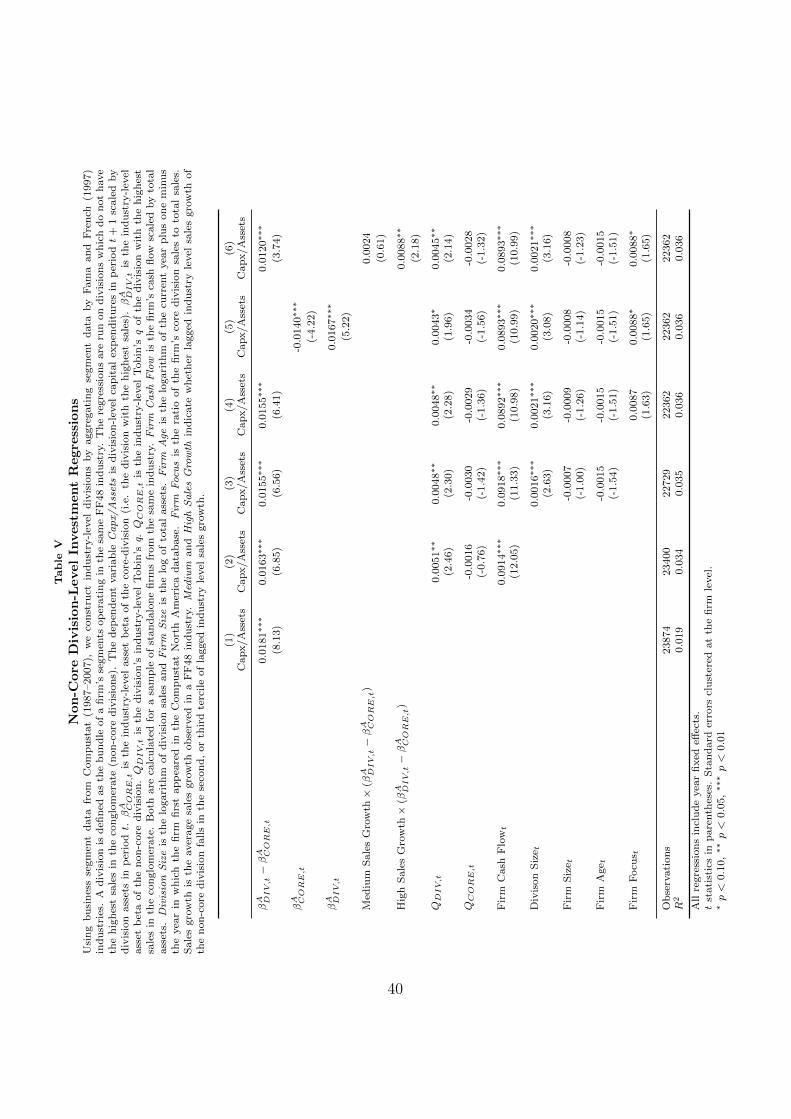
We then report multivariate regression results in Table V, in order to

control more extensively for observable determinants of investment. Stan-

dard errors are clustered at the firm-level. In unreported regressions we also

cluster standard errors at the non-core division level which leaves our results

unaffected. Column (1) establishes the basic fact by showing that non-core

division investment depends positively on the spread between the non-core

15

and the core division’s industry betas. The larger the spread, the higher the

investment in the respective non-core division. This is precisely what would

be expected if companies discount risky projects using too low discount rates.

The estimated order of magnitude is non-negligible: a one standard deviation

increase in the beta spread (0.35) leads to an investment increase by 0.7% of

division assets. This is equivalent to 10% of the average investment rate.

[Table V about here.]

In column (2), we add the main determinants of corporate investment,

i.e. industry-level Tobin’s q ’s of the core and the non-core divisions, as well

as cash flows (at the firm level). We control for the investment opportunities

of both the core and the non-core divisions in order to address the concern

that asset betas may correlate with variations in investment opportunities

that are not captured by Tobin’s q ’s. After including these controls, the

coefficient estimate for the spread decreases slightly but remains highly sta-

tistically significant. Columns (3) and (4) add other potential determinants

of division level investment, i.e. Division Size, Firm Size, Firm Age and a

measure of Firm Focus to the specification. Our results remain unchanged.

In unreported regressions, we have also sought to replace industry-level To-

bin’s q by a division level measure of investment opportunities, i.e. lagged

sales growth. Again, our results remain robust in this alternative specifica-

tion. In column (5) we replace the spread by its two separate components

βACORE,t and βADIV,t. The results show a negative sign for the coefficient esti-

mate for βACORE,t and a positive sign for βADIV,t. This suggests that whenever

the company has a low risk core activity (low βACORE,t), and therefore a low

16

hurdle rate, it is inclined to invest more strongly in non-core divisions with a

higher asset risk. The fact that βACORE,t is significant provides strong evidence

that diversified companies look at divisions belonging to industries different

from their core activity with the eyes of their core industry’s characteristics.

In terms of magnitude, the investment distortion we document is quite im-

portant. Assume βADIV,t−βACORE,t = 0.35, which is about one sample standard

deviation. This means the gap in discount rates between the division and its

core is approximately 2% (assuming a 6% equity risk premium). Given our

estimates, we would expect the non-core division’s investment rate to be 0.5

(0.0155*0.35) percentage points higher. This is a non-negligible effect: the

median non-core division investment rate is about 4 % in our data.

Last, we expect the documented investment distortion to be larger if the

project’s sales growth is bigger. To see this, assume, in the spirit of Gordon

and Shapiro (1956), that an investment project in a non-core division pays

a cash flow C, with constant growth rate g smaller than the WACC. Then,

the present value of the project is given by CWACC−g . From this formula, it is

obvious that the valuation mistake made by not choosing the right WACC is

bigger when g is larger, in a convex fashion.4 Hence, we expect the impact of

beta spread on investment to be bigger when the division belongs to a fast

growing industry.

Column (6) of Table V reports the outcome of such a consistency check.

We code an indicator variable for each tercile of lagged industry sales growth

(Low, Medium and High Growth) and interact these dummies with the spread

4To see this formally, assume that the conglomerate chooses WACC − δ instead ofWACC, where δ is small. Then, the estimated present value of the project is inflated byδ × C

(WACC−g)2 , which is increasing and convex in g.

17

in asset betas. The results show that while investment of medium growth

non-core divisions are not significantly more sensitive to the spread than low

growth divisions (Medium Growth × (βADIV,t − βACORE,t) is not significant),

high growth divisions turn out to be significantly more sensitive to the spread

than low growth divisions (t-stat 2.18). The difference is large too: while for

divisions in the bottom tercile of industry growth, the coefficient is equal to

0.012, it is equal to 0.021 in the top tercile. The estimated effect is therefore

twice as large. This underlines the idea that the investment sensitivity is in

fact convex in lagged sales growth.

II.2 Robustness Checks

Our sample includes all industries, even the financial sector. We have good

reasons to believe that even the banking sector can be “WACC fallacious”,

which is why we did not remove the financial sector from our main specifi-

cations. There might, however, be concerns that investment and investment

opportunities are not well captured in Compustat. To check that our results

do not depend on the inclusion of the financial sector, we have replicated

the results of Table V, excluding Banking and Insurance (FF48 industries 44

and 45). We report these new estimates in Table A.II. They are, if anything,

stronger, consistent with the fact that accounting data are noisier in these

industries.

We report further robustness checks in Table VI. First, in column (1), we

seek to account for the fact that, as noticed before, instead of using the cost

of capital of the division, conglomerates may be using a firm-wide average

18

asset beta. In column (1), we thus use as regressor the weighted average

division asset beta, where the weights correspond to the ratio of division

to total firm assets. As expected, the coefficient estimate is significantly

negative in this specification too. To distinguish between the two stories, we

run in column (2) a regression with both the average firm beta and the beta

of the core division. In this specification, the average beta of the firm is no

longer significant. The documented investment distortion thus seems to be

driven by the use of the core-division’s discount rate rather than the use of

an average firm-wide WACC, even though both hypotheses may ultimately

be hard to distinguish rigorously.

[Table VI about here.]

In column (3), we seek to directly address the concern that the beta

spread may capture differences in investment opportunities between the di-

vision and the core, that is not fully controlled for by the Tobin’s q ’s. We do

so by including the gap between the division-level’s and the firm’s overall To-

bin’s q. It leaves the estimated effect of beta spread unaffected. In the same

spirit, the beta spread may simply capture a measure of diversity of a firm’s

investment opportunities, which has been shown in earlier work to distort in-

vestment behavior (Rajan et al. (2000)). In column (4), we therefore include

as additional control the within-firm standard deviation of industry-level To-

bin’s q ’s normalized by firm wide q. As found by Rajan et al. (2000), the

more diverse the firm’s investment opportunities, the lower non-core division

investment on average. Yet, the inclusion of the diversity control and the gap

between the division and the firm’s Tobin’s q does not affect our conclusions.

19

In column (5), we control for firm-wide investment policy through includ-

ing the core division’s investment rate. This control variable also leaves the

coefficient estimates for both βACORE,t and βADIV,t unchanged.

In column (6), we are looking at the sources of identification. To do this,

we include division industry-year fixed-effects. In this regression, the iden-

tification is purely based on the comparison between divisions in the same

industry, depending on whether they are affiliated with low or high beta core

divisions. The estimated effect of βACORE,t is divided by two but remains

statistically significant at the 5% significance level. Hence, the estimate of

βACORE,t is identified both on the within industry, across conglomerates vari-

ation, and on investment variability across industries. Finally, we control

for firm fixed effects (see column (7)). After controlling for firm fixed ef-

fects, we still find evidence of an investment bias toward riskier non-core

divisions (significant coefficient for βADIV,t). By contrast, βACORE,t is no longer

significant.

One last concern with our results is that we may be capturing the impact

of upstream integration. Assume, for instance, that a firm produces toys and

owns trucks to transport them. It therefore has two activities: transportation

(non-core) and toy-production (core). If the cost of capital in the toy industry

goes down, the firm may expand its production capacity, for instance to cater

to investor sentiment (for this to hold, note that the beta must be capturing

investment determinants not already controlled for in our regressions). To

ship the additional production, it will also invest in new trucks. In this

setting, investment in a non-core division (trucks) responds to changes in the

WACC of the core division (toys), for reasons that have little to do with the

20

WACC fallacy.

[Table VII about here.]

To address this concern, we construct a measure of vertical integration

between each non-core division and its core, and interact this measures with

the beta spread to see if it affects the relation estimated in Table V. For

each FF48 industry, we calculate (1) the fraction of this industry’s output

that is sold to each (downstream) FF48 industry and (2) the fraction of this

industry’s input that comes from each (upstream) industry. For each indus-

try pair (i, j), Vij is equal to the mean of these two numbers, and therefore

measures the extent to which these two industries are integrated both up-

stream and downstream. For each non-core division, we split the measure

of relatedness with the core into three tercile dummies, and interact them

with the beta spread. We report the estimates using various specifications in

Table VII. In column (1), we report the baseline result without interaction.

In column (2), we add the interaction terms between beta spread and the

dummies. It appears that the measured impact of beta spread on investment

does not depend on the extent to which the non-core division is related with

its core. In columns (3) and (4), we interact the two measures of growth

opportunities with the relatedness dummies. The overall diagnosis remains:

our estimated effect of beta spread on investment is not driven by non-core

divisions that are vertically related to the core activity.

21

II.3 Evidence of bounded rationality

Taking the wrong cost of capital destroys present value, because it biases

the firm’s investment decisions away from value maximization. On the other

hand, computing the adequate cost of capital, making it vary across projects,

making sure that division managers do not manipulate it to defend low NPV

projects, is also costly. Sometimes, it may therefore be optimal to keep a

single WACC for the entire organization. But if the costs of doing so are too

high, we expect firms to use different WACCs. This “bounded rationality

view” makes predictions as to which firms are “WACC fallacious” and which

firms are not: the relationship uncovered in Table V should disappear when

the benefits of taking the right WACC are large.

[Table VIII about here.]

In this Section, we test the “bounded rationality view”. We do this by

interacting beta spread with measures of the net benefit of adopting differen-

tiated WACCs. Bounded rationality predicts that investment policy should

be less sensitive to beta spread when this net benefit is high (i.e. when firms

find it optimal to unbias themselves). We report the results of this investi-

gation in Table VIII using four different measures of net benefit to take the

right WACC. In column (1), we first hypothesize that financial knowledge

of corporate decision makers in charge of making capital budgeting decisions

has improved over time. Higher financial sophistication of managers due to

MBA style education could thus have improved the quality of capital alloca-

tion decisions within conglomerate firms, making the cognitive cost of taking

the right WACC decrease over time. We therefore expect the sensitivity of

22

investment to beta spread to decrease over time, and test this by interacting

four period dummies (1987-1991, 1992-1996, 1997-2001, 2002-2007) with beta

spread. The analysis by sub-period indicates that the investment distortion

has been strongest between 1987 and 1996.5

In columns (2)–(4), we use cross-sectional proxies of net benefit of fi-

nancial sophistication. In column (2), we use the Relative Importance of a

non-core division. The idea is that, when the non-core division is large with

respect to the core, valuation mistakes have larger consequences; these di-

visions are therefore less likely to be “WACC fallacious”. We calculate this

measure by scaling non-core division sales by the sales of the core division.

Values close to one indicate that the non-core division in question is almost

as important as the core-division within the conglomerate. By contrast, val-

ues close to zero indicate that the non-core division is negligible vis a vis the

core division. We then split this measure into terciles and interact it with

the beta spread. We report the regression results in column (2): investment

in large divisions is less sensitive to beta spread, suggesting that investment

in relatively large divisions is less “WACC fallacious”. In column (3), the

measure of net benefit is diversity of costs of capital, defined at the firm level

as the within-firm standard deviation of (core and non-core) division asset

betas. Again, the intuition is that taking a single WACC to evaluate invest-

ment projects leads to larger mistakes if costs of capital are very different

within the organization. As before, we split our measure of diversity into

5Interestingly, the change in business segment reporting standards initiated by theFASB issuance of SFAS 131 in June 1997 does not seem to have an impact on our results,since our coefficients remain statistically significant also in sub-periods following the changein regulation.

23

terciles. Column (3) shows that division investment in firms with highly di-

verse costs of capital is significantly less sensitive to the beta spread. These

firms therefore seem to find it optimal to use different WACCs. Last, we

explore in column (4) the role of CEO ownership: here the intuition is that

CEOs with more “skin in the game” will find it more profitable to avoid

value destroying investment decisions and will opt for financial sophistica-

tion in the organization she’s running. This is consistent with Baker et al.

(2007), who note that in order for irrational managers to have an impact on

corporate policies, corporate governance should be somewhat limited. Be-

cause of the limited availability of this variable, we only split CEO ownership

into two dummies (above and below 1%, the sample median). We show, in

column (4), that the impact of beta spread on division investment is divided

by three for firms whose CEO has a relatively larger stake. Such evidence

is also in line with evidence in Ozbas and Scharfstein (2010), who find that

inefficient investment in conglomerates decreases with management equity

ownership.

III Efficiency effects

In this section, we examine the efficiency costs of using the “wrong” cost

of capital. Doing this is difficult in the context of conglomerate investment,

since we would need to compare firm values in the cross-section. A more

powerful test, which we implement here, consists of looking at market re-

action to large investment projects, whose cost of capital we can measure.

To do this, we study diversifying mergers and acquisitions. For our pur-

24

pose, these investment projects have four advantages. First, they are easy

to observe: large standard datasets report the exact date, the size, industry

and the amount invested in these projects. Second, the cost of capital of

the acquisition can be computed (using the target’s industry cost of capital)

and is, for diversifying acquisitions, different from the cost of capital of the

acquirer, which may give rise to “WACC fallacious” behavior. Third, we

have a reasonable estimate of their NPV, namely, the stock price reaction

of the acquirer upon acquisition announcement. Under the assumption that

markets are efficient, the announcement returns provides an estimate of the

NPV created by the project. Last, these projects tend to be large enough

so that their impact on the market value of the acquirer is detectable in a

credible way.

III.1 WACC fallacious acquisitions

We first check that acquisitions are subject to the same WACC fallacy as

non-core division investment. From Table III, Panel B, we see that, across

all deals in our sample, the beta spread is on average -0.05: targets have,

on average, a higher asset beta than bidders. The difference is statistically

significant at 1%. This is consistent with bidders using their own discount

rate to value targets: this leads to overvaluation from the bidder’s side, which

makes the deal more likely to succeed. From Table III, Panel B, we also

observe that this phenomenon is more pronounced when the target is private

than when it is public. This is consistent with the “bounded rationality”

hypothesis defended in the previous section: when the target is publicly

25

listed, information about its true value is cheaper to come by (the market

quotes a price). As a result, it is easier to make the right estimate.

III.2 Value loss in diversifying asset acquisitions

The fallacy of using inadequate discount rates is expected to have implica-

tions for bidder abnormal returns around the announcement of diversifying

acquisitions. Whenever bidders use too high a discount rate, they are more

likely to undervalue their targets and therefore more likely to propose an

offer price for the target’s assets below fair value. Shareholders of the bidder

should thus perceive a bid from a high beta bidder for a low beta target

as relatively better news, since it reduces the likelihood of overpaying for

the target. Conversely, a low industry-level beta bidder should have a ten-

dency to overvalue high beta assets. Hence, the bid announcement from a

low industry-level asset beta company for a high beta industry asset should

be perceived as bad news by stock markets because the bidder is paying too

much. We thus expect bidder abnormal returns around transactions to be

significantly higher whenever the bidder’s WACC is higher than that of the

target.

[Figure 2 about here]

In Figure 2, we plot the mean cumulative abnormal returns of bidders

around the announcement of diversifying asset acquisitions conditional on

whether the bidder’s WACC is lower or higher than that of the target. Ab-

normal returns are calculated as market adjusted returns on the respective

26

event day. We use the CRSP Value Weighted Index as the market bench-

mark. For both categories of deals, we first see that announcement returns

are positive: this is consistent with Bradley and Sundaram (2006) who find

that announcement returns for acquirers of private firms (the vast major-

ity of the deals in our sample) are positive and statistically significant (see

also Betton et al. (2008)). More importantly to us, evidence from Figure 2

suggests that the market welcomes bids involving low beta bidders and high

beta targets less favorably than bids with high beta bidders and low beta

targets. This confirms our hypothesis that low beta bidder tend to overbid

for high beta targets.

In order to formally test whether this difference is statistically significant,

we regress both the abnormal return on the announcement day (AR(0)),

as well as the seven day cumulative abnormal return surrounding the an-

nouncement (CAR(3,3)) on a dummy variable indicating whether the bid-

der’s WACC exceeds that of the target. The results from regressions in

which the abnormal return serves as the dependent variable are reported in

table IX. Table X reports the regression results for the cumulative abnormal

return (CAR(-3,3)). In all specifications, we also include year dummies to

capture the potential impact of merger waves on announcement returns and

control for the size of the transaction, which we calculate as the natural log

of the deal value as disclosed by SDC. In order to control for deals that are

announced on the same day, standard errors are clustered by announcement

dates. In unreported regressions we cluster standard errors by week, month

and year, which does not affect our results.

27

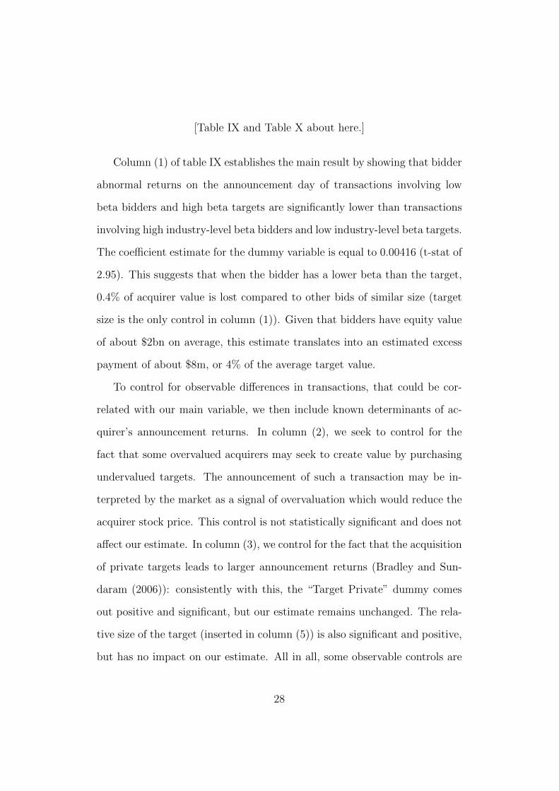
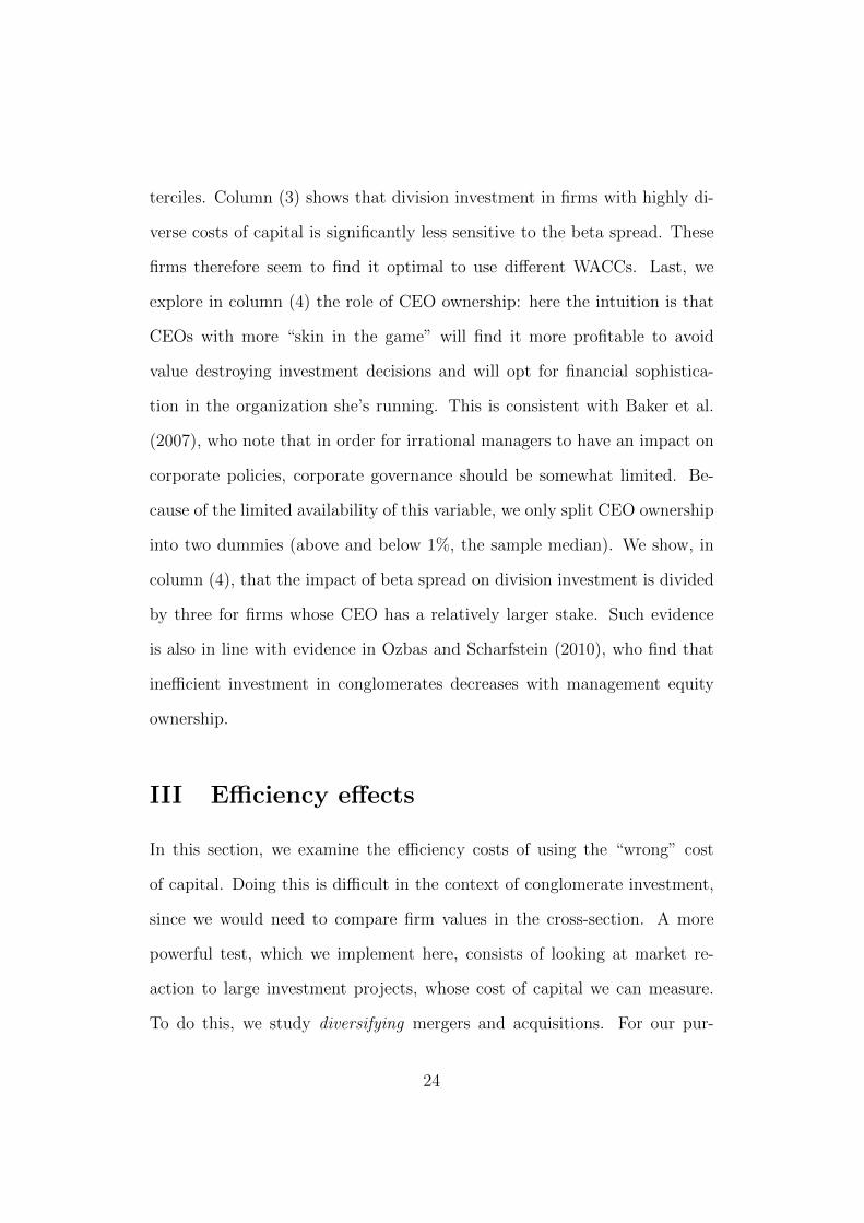
[Table IX and Table X about here.]

Column (1) of table IX establishes the main result by showing that bidder

abnormal returns on the announcement day of transactions involving low

beta bidders and high beta targets are significantly lower than transactions

involving high industry-level beta bidders and low industry-level beta targets.

The coefficient estimate for the dummy variable is equal to 0.00416 (t-stat of

2.95). This suggests that when the bidder has a lower beta than the target,

0.4% of acquirer value is lost compared to other bids of similar size (target

size is the only control in column (1)). Given that bidders have equity value

of about $2bn on average, this estimate translates into an estimated excess

payment of about $8m, or 4% of the average target value.

To control for observable differences in transactions, that could be cor-

related with our main variable, we then include known determinants of ac-

quirer’s announcement returns. In column (2), we seek to control for the

fact that some overvalued acquirers may seek to create value by purchasing

undervalued targets. The announcement of such a transaction may be in-

terpreted by the market as a signal of overvaluation which would reduce the

acquirer stock price. This control is not statistically significant and does not

affect our estimate. In column (3), we control for the fact that the acquisition

of private targets leads to larger announcement returns (Bradley and Sun-

daram (2006)): consistently with this, the “Target Private” dummy comes

out positive and significant, but our estimate remains unchanged. The rela-

tive size of the target (inserted in column (5)) is also significant and positive,

but has no impact on our estimate. All in all, some observable controls are

28

statistically significant, but our estimate resists well.

Findings of table IX are confirmed by results reported in table X, which

looks at cumulative returns 7 days around the announcement date (CAR(3,3)).

These estimates are larger: The coefficient estimate for the dummy variable

capturing differences in the cost of capital between the target and the bid-

der is now equal, across specifications to about 0.7% of the acquirer’s value.

This is in line with the idea that announcements take several days to be im-

pounded into prices. For the average acquirer, whose market capitalization

is about $2bn, this suggests a value loss of about $14m, or 7% of the value

of the average target (whose average value is approximately $200m).

IV Conclusion

Survey evidence suggests that many firms use a firm-wide discount rate

to evaluate projects (Graham and Harvey (2001)). The prevalence of this

”WACC fallacy” implies that firms tend to bias investment upward for di-

visions that have a higher industry beta than the firm’s core division. This

paper provides a direct test of this prediction using segment-level accounting

data. We find a robust positive relationship between division-level investment

and the spread between its industry beta and the beta of the firm’s core di-

vision. Using unrelated data on mergers and acquisitions, we also find that

the acquirer’s stock-price reaction to the announcement of an acquisition is

lower when the target has a higher beta than the acquirer. The prevalence of

the ”WACC fallacy” among corporations seems consistent with managerial

bounded rationality. It is actually not so simple to explain to a non-finance

29

executive why it is logically flawed for a firm to discount a risky project us-

ing its own cost of capital. The costs associated with using multiple discount

rates might, however, not be purely cognitive or computational: They might

also be organizational, as the use of multiple discount rates might increase

the scope for politicking and gaming of the capital budgeting process in a

hierarchy, in the spirit of Rajan et al. (2000); Scharfstein and Stein (2000).

30

References

Baker, M., Ruback, R., and Wurgler, J. (2007). Behavioral Corporate Fi-nance. Handbook of corporate finance: Empirical corporate finance, 1:145–86.

Berger, P. and Ofek, E. (1995). Diversification’s effect on firm value. Journalof Financial Economics, 37(1):39–65.

Bertrand, M. and Schoar, A. (2003). Managing with Style: The Effect ofManagers on Firm Policies. Quarterly Journal of Economics, 118(4):1169–1208.

Betton, S., Eckbo, B., and Thorburn, K. (2008). Corporate Takeovers. Hand-book of Corporate Finance: Empirical Corporate Finance, 2(15):291–430.

Bierman, J. H. (1993). Capital budgeting in 1992: a survey. FinancialManagement, 22(3):24.

Bradley, M. and Sundaram, A. (2006). Acquisition and performance: A re-assessment of the evidence. Working Paper, Fuqua School of Business,Duke University.

Brealey, R., Myers, S., and Allen, F. (2005). Principles of Corporate Finance,McGraw-Hill, New York. McGraw-Hill, New-York, NY.

Fama, E. and French, K. (1997). Industry costs of equity. Journal of Finan-cial Economics, 43(2):153–193.

Fan, J. and Lang, L. (2000). The Measurement of Relatedness: An Applica-tion to Corporate Diversification. Journal of Business, 73(4):629–660.

Gabaix, X. (2010). A Sparsity-Based Model of Bounded Rationality. WorkingPaper, Stern School of Business, New York University.

Gompers, P., Ishii, J., and Metrick, A. (2003). Corporate Governance andEquity Prices. Quarterly Journal of Economics, 118(1):107–155.

Gordon, M. and Shapiro, E. (1956). Capital Equipment Analysis: The Re-quired Rate of Profit. Management Science, 3(1):102–110.

Graham, J. and Harvey, C. (2001). The theory and practice of corporatefinance: evidence from the field. Journal of Financial Economics, 60(2-3):187–243.

31

Graham, J., Harvey, C., and Puri, M. (2010). Capital Allocation and Dele-gation of Decision-Making Authority within Firms. Working Paper, FuquaSchool of Business, Duke University.

Grinblatt, M. and Titman, S. (2002). Financial Markets and Corporate Strat-egy. McGraw-Hill, New-York, NY.

Kaplan, S. and Zingales, L. (1997). Do Investment-Cash Flow SensitivitiesProvide Useful Measures of Financing Constraints? Quarterly Journal ofEconomics, 112(1):169–215.

Lamont, O. (1997). Cash Flow and Investment: Evidence from InternalCapital Markets. Journal of Finance, 52(1):83–109.

Landier, A. and Thesmar, D. (2009). Financial Contracting with OptimisticEntrepreneurs. Review of Financial Studies, 22(1):117.

Malmendier, U. and Tate, G. (2005). CEO Overconfidence and CorporateInvestment. The Journal of Finance, 60(6):2661–2700.

Malmendier, U. and Tate, G. (2008). Who makes acquisitions? CEO over-confidence and the market’s reaction. Journal of Financial Economics,89(1):20–43.

Modigliani, F. and Miller, M. (1958). The Cost of Capital, CorporationFinance and the Theory of Investment. The American Economic Review,48(3):261–297.

Montgomery, C. and Wernerfelt, B. (1988). Diversification, Ricardian rents,and Tobin’s q. The RAND Journal of Economics, 19(4):623–632.

Morck, R., Shleifer, A., and Vishny, R. (1990). Do Managerial ObjectivesDrive Bad Acquisitions? Journal of Finance, 45(1):31–48.

Ozbas, O. and Scharfstein, D. (2010). Evidence on the Dark Side of InternalCapital Markets. Review of Financial Studies, 23(2):581.

Poterba, J. and Summers, L. (1995). A CEO survey of US companies’ timehorizons and hurdle rates. Sloan Management Review, 37(1):43.

Rajan, R., Servaes, H., and Zingales, L. (2000). The Cost of Diversity:The Diversification Discount and Inefficient Investment. The Journal ofFinance, 55(1):35–80.

32

Scharfstein, D. and Stein, J. (2000). The Dark Side of Internal CapitalMarkets: Divisional Rent-Seeking and Inefficient Investment. The Journalof Finance, 55(6):2537–2564.

Shin, H. and Stulz, R. (1998). Are Internal Capital Markets Efficient? Quar-terly Journal of Economics, 113(2):531–552.

33

Figures

Figure 1. Monotonicity of Excess Investment. We fit an Investment equation for all standalonefirms. The specification we chose is Invi,t+1 = f(QIND

it , sizeit, cashflowit)+εit. In the case of standalone

firms, investment, Tobin’s q, size and cash flows are equal at the firm and the division level i and j. QINDi,t

is the industry level Tobin’s q of the standalone firm, sizeit the natural logarithm of the firm’s assets, andcashflowit the firm wide cash flow. We use the estimated coefficients in order to predict the investmentrate for all non-core divisions of conglomerates. In predicting the non-core division investment ˆInvj,t+1,we use the firm wide cashflowit, the natural log of the division’s assets sizejt as well as the industry levelTobin’s q of the industry the non-core division belongs to, i.e. QIND

jt . Excess investment for non-core

divisions is the difference between observed and predicted investment, that is εjt = Invjt − ˆInvjt. Thegraph plots the average predicted excess investment εjt by deciles of βA

DIV − βACORE .

34

Figure 2. Bidder Cumulative Abnormal Returns (All Acquisitions). Mean cumulative abnormalreturns of the bidder around the announcement of an asset acquisition conditional on whether the WACCof the bidder exceeds that of the target. Only diversifying acquisitions in which the acquiring firm’s Famaand French (1997) industry differs from that of the target are considered. Abnormal returns are marketadjusted and calculated as the difference between the acquiring firm’s daily stock return and the CRSPValue Weighted Market Return on the respective event day. All transactions between 1988 and 2007fulfilling the sample construction conditions are considered (N=6,206).

35

Tables

Table I

Firm-Level Descriptive StatisticsThis table reports descriptive statistics of the employed firm-level variables. Variables based on datafrom Compustat and CRSP are observed for the period of 1987 to 2007. CEO related variablesfrom Compustat Execucomp are observed from 1992 to 2007 only. All variables are defined in theAppendix, except for betas, which are defined in the text (see section I.3). Standalone firms arefirms with activities concentrated in a single FF48 industry, whereas Conglomerate Firms are diver-sified across at least two different FF48 sectors. All variables are winsorized at the first and 99th percentile.

Standalone Firms

Mean Median SD P25 P75 N

Firm Cash Flowt 0.03 0.06 0.17 -0.01 0.12 107784

Firm Sizet 4.30 4.28 2.46 2.63 5.94 122120

Firm Aget 2.04 2.08 0.98 1.39 2.77 119087

Firm Investmentt 0.06 0.04 0.07 0.01 0.08 118351

Leveraget 0.19 0.09 0.24 0.00 0.30 121023

Salest 3.94 4.10 2.66 2.35 5.75 122178

Sales Growtht 0.13 0.09 0.37 -0.04 0.26 105336

QFIRM,t 1.88 1.42 1.27 1.04 2.27 93558

βAAV ERAGE,t 0.65 0.62 0.34 0.41 0.85 106541

CEO Share Ownership 5.20 1.58 8.59 0.52 5.70 11463

Conglomerate Firms

Mean Median SD P25 P75 N

Firm Cash Flowt 0.06 0.07 0.10 0.04 0.11 16185

Firm Sizet 5.93 6.01 2.44 4.14 7.73 16543

Firm Aget 2.79 3.04 0.93 2.20 3.53 16442

Firm Investmentt 0.06 0.05 0.05 0.03 0.07 16252

Leveraget 0.23 0.20 0.20 0.07 0.33 16502

Number of Divisionst 2.56 2.00 0.87 2.00 3.00 16543

Salest 5.84 6.04 2.41 4.20 7.57 16543

Sales Growtht 0.10 0.07 0.26 -0.02 0.18 15749

Firm Focust 0.73 0.74 0.17 0.59 0.88 16460

QFIRM,t 1.49 1.22 0.84 1.01 1.65 14033

SD(QDIV,t)/QFIRM,t 0.23 0.18 0.19 0.09 0.32 13994

βAAV ERAGE,t 0.56 0.55 0.24 0.41 0.69 15831

CEO Share Ownership 5.71 1.60 9.94 0.54 5.80 1633

36

Table II

Non-Core Division-Level Descriptive StatisticsThis table reports summary statistics of variables at the non-core division-level for the sample period of1987–2007. Non-core divisions are divisions that do not have the highest sales within the Conglomeratefirm. Divisions are defined by grouping together segments operating in the same Fama and French (1997)industry category. All variables are winsorized at the first and 99th percentile and are defined in theAppendix.

Mean Median SD P25 P75 N

Capx/Assets 0.06 0.04 0.07 0.01 0.09 23871

Divison Sizet 4.07 4.26 2.54 2.44 5.87 23269

QDIV,t 1.72 1.63 0.42 1.43 1.93 23858

QCORE,t 1.68 1.61 0.42 1.41 1.92 23831

QDIV,t −QCORE,t 0.03 0.03 0.51 -0.27 0.33 23818

QDIV,t −QFIRM,t 0.26 0.38 0.84 0.02 0.70 20163

βEDIV,t 1.08 1.09 0.28 0.92 1.25 23871

βECORE,t 1.04 1.08 0.31 0.88 1.23 23871

βADIV,t 0.56 0.54 0.29 0.36 0.72 23871

βACORE,t 0.55 0.53 0.27 0.37 0.69 23871

βADIV,t − βA

CORE,t 0.01 0.01 0.35 -0.21 0.22 23871

Investment Core Divisiont 0.07 0.05 0.09 0.02 0.09 18715

Divison Sales Growtht 0.46 0.06 13.29 -0.06 0.20 17786

Divison Industry-Level Sales Growtht 0.10 0.11 0.09 0.05 0.15 23871

VDIV,t 0.04 0.03 0.04 0.01 0.06 23871

Relative Importancet 0.31 0.24 0.27 0.09 0.49 23871

37

Table

III

DescriptiveSta

tisticsofDeal,

Bidderand

Targ

etChara

cteristics

Th

ista

ble

show

sd

escr

ipti

ve

stati

stic

sof

dea

l,b

idd

eran

dta

rget

chara

cter

isti

csfo

rou

rsa

mp

leof

6,2

06

div

ersi

fyin

gtr

an

sact

ion

s.A

div

ersi

fyin

gtr

ans-

act

ion

isa

com

ple

ted

mer

ger

or

acq

uis

itio

nin

wh

ich

the

bid

der

has

succ

essf

ully

sou

ght

contr

ol

of

ata

rget

not

bel

on

gin

gto

its

ow

nF

F48

ind

ust

ry.

(βA BID

DER

−βA TARGET>

0)

ind

icate

sw

het

her

the

diff

eren

ceb

etw

een

the

bid

der

’san

dth

eta

rget

’sass

etb

etas

isp

osi

tive.

(QBID

DER

−Q

TARGET>

0)

isa

du

mm

yvari

ab

lein

dic

ati

ng

wh

eth

erth

ed

iffer

ence

bet

wee

nth

eb

idd

er’s

an

dth

eta

rget

’sin

du

stry

level

Tob

in’s

q’s

isp

osi

tive.VTARGET

isth

evalu

eof

the

tran

sact

ion

as

dis

close

dby

SD

C(i

nM

illion

US

-$).E

BID

DER

isth

efi

scalyea

ren

deq

uit

ym

ark

etvalu

eofth

eb

idd

erin

the

yea

rp

rior

toth

eb

idan

nou

nce

men

t(i

nM

illion

US

-$).

Ta

rget

pri

vate

?is

ad

um

my

vari

ab

lein

dic

ati

ng

wh

eth

erth

eta

rget

isa

pri

vate

com

pany

an

dT

end

erO

ffer

?in

dic

ate

sw

het

her

the

bid

der

sou

ght

contr

olth

rou

gh

the

pro

cess

of

ate

nder

off

er.

All

Ca

sh?

isa

du

mm

yvari

ab

leth

at

takes

on

the

valu

eon

ew

hen

the

con

sid

erati

on

was

enti

rely

paid

inca

shw

her

eas

All

Equ

ity?

takes

on

the

valu

eofon

ew

hen

ever

the

targ

et’s

share

hold

ers

are

enti

rely

com

pen

sate

dw

ith

share

s.M

ult

i-D

ivis

ion

Acq

uir

er?

takes

on

the

valu

eofon

ew

hen

the

bid

der

’sb

usi

nes

sact

ivit

ies

are

div

ersi

fied

acr

oss

at

least

two

mu

ltip

leF

F48

ind

ust

ryca

tegori

es.

Ho

stil

ean

dC

ha

llen

gin

gB

id?

are

two

du

mm

yvari

ab

les

ind

icati

ng

wh

eth

erth

eb

id’s

natu

reis

host

ile

an

dw

het

her

ther

eh

as

bee

na

chall

engin

gb

id.βA i

isth

ein

du

stry

level

ass

etb

eta

an

dQ

ith

ein

du

stry

-lev

elT

ob

in’s

q.

Pan

elA

:D

eal

Ch

ara

cter

isti

cs

All

Deals

(N=6206)

PublicTargets

(N=656)

Private

Targets

(N=5500)

(βA BID

DER−βA TARGET>

0)

0.4

10.4

60.4

0(0

.49)

(0.5

0)

(0.4

9)

(QBID

DER−Q

TARGET>

0)

0.5

40.4

80.5

5(0

.50)

(0.5

0)

(0.5

0)

VTARGET

186.1

3799.4

2113.6

4(1

074.8

7)

(2977.5

1)

(442.4

2)

EBID

DER

1917.2

65668.0

31473.9

2(7

718.5

8)

(14493.8

6)

(6321.6

4)

VTARGET/E

BID

DER

0.4

10.3

90.4

2(7

.77)

(0.7

1)

(8.2

1)

Targ

etp

rivate

?0.8

90.0

01.0

0(0

.31)

(.)

(.)

Ten

der

Off

er?

0.0

30.2

30.0

0(0

.17)

(0.4

2)

(.)

All

Cash

?0.3

10.4

10.3

0(0

.46)

(0.4

9)

(0.4

6)

All

Equ

ity?

0.1

20.2

70.1

1(0

.33)

(0.4

4)

(0.3

1)

Mu

lti-

Div

isio

nA

cqu

irer

?0.3

10.4

80.2

8(0

.46)

(0.5

0)

(0.4

5)

Host

ile

Bid

?0.0

00.0

20.0

0(0

.05)

(0.1

2)

(0.0

2)

Ch

allen

gin

gB

id?

0.0

10.0

60.0

0(0

.09)

(0.2

4)

(0.0

4)

Pan

elB

:B

idd

eran

dT

arg

etC

hara

cter

isti

cs

All

Deals

(N=6206)

PublicTargets

(N=656)

Private

Targets

(N=5500)

Bid

der

Targ

etD

iffB

idd

erT

arg

etD

iffB

idd

erT

arg

etD

iffβA i

0.5

90.6

4-0

.05∗∗

∗0.6

80.7

0-0

.02∗

0.5

80.6

3-0

.05∗∗

∗

(0.4

0)

(0.3

4)

(0.4

0)

(0.3

6)

(0.3

3)

(0.3

9)

(0.4

0)

(0.3

4)

(0.4

0)

Qi

1.8

71.8

60.0

11.8

91.9

1-0

.03

1.8

71.8

60.0

1∗∗

(0.4

5)

(0.4

6)

(0.4

9)

(0.4

9)

(0.5

1)

(0.5

2)

(0.4

4)

(0.4

6)

(0.4

9)

Sta

nd

ard

dev

iati

on

sin

pare

nth

eses

∗p<

0.1

0,∗∗p<

0.0

5,∗∗

∗p<

0.0

1

38

Table IV

Diversifying Transactions Sample by Calendar YearThis table shows the temporal distribution of the sample of diversifying mergers and acquisitions. Yearlymeans and standard deviations of the nominal deal value (In Million US-$) are calculated by relying onthe deal value as disclosed by SDC.

# of Acquisitions Mean Value (Million US-$) SD

1988 98 218.52 614.30

1989 133 195.57 666.76

1990 121 78.94 317.95

1991 109 47.72 83.77

1992 162 51.73 121.32

1993 234 56.36 152.75

1994 316 81.10 295.22

1995 332 153.09 1121.65

1996 467 126.55 609.68

1997 679 122.92 410.24

1998 740 138.86 526.48

1999 428 264.66 1231.43

2000 350 371.23 1772.37

2001 222 181.40 422.21

2002 255 142.14 453.85

2003 267 168.51 534.73

2004 279 193.12 424.56

2005 364 401.60 2941.85

2006 367 310.91 1532.03

2007 283 249.94 581.31

Total 6206 186.13 1074.87

39

Table

V

Non-C

ore

Division-L

evelIn

vestmentRegre

ssions

Usi

ng

bu

sin

ess

segm

ent

data

from

Com

pu

stat

(1987–2007),

we

con

stru

ctin

du

stry

-lev

eld

ivis

ion

sby

aggre

gati

ng

segm

ent

data

by

Fam

aan

dF

ren

ch(1

997)

ind

ust

ries

.A

div

isio

nis

defi

ned

as

the

bu

nd

leof

afi

rm’s

segm

ents

op

erati

ng

inth

esa

me

FF

48

ind

ust

ry.

Th

ere

gre

ssio

ns

are

run

on

div

isio

ns

wh

ich

do

not

have

the

hig

hes

tsa

les

inth

eco

nglo

mer

ate

(non

-core

div

isio

ns)

.T

he

dep

end

ent

vari

ab

leC

ap

x/A

sset

sis

div

isio

n-l

evel

cap

ital

exp

end

itu

res

inp

erio

dt

+1

scale

dby

div

isio

nass

ets

inp

erio

dt.βA CORE,t

isth

ein

du

stry

-lev

elass

etb

eta

of

the

core

-div

isio

n(i

.e.

the

div

isio

nw

ith

the

hig

hes

tsa

les)

.βA DIV,t

isth

ein

du

stry

-lev

elass

etb

eta

of

the

non

-core

div

isio

n.Q

DIV,t

isth

ed

ivis

ion

’sin

du

stry

-lev

elT

ob

in’s

q.Q

CORE,t

isth

ein

du

stry

-lev

elT

ob

in’s

qof

the

div

isio

nw

ith

the

hig

hes

tsa

les

inth

eco

nglo

mer

ate

.B

oth

are

calc

ula

ted

for

asa

mp

leof

stan

dalo

ne

firm

sfr

om

the

sam

ein

du

stry

.F

irm

Ca

shF

low

isth

efi

rm’s

cash

flow

scale

dby

tota

lass

ets.

Div

isio

nS

ize

isth

elo

gari

thm

of

div

isio

nsa

les

an

dF

irm

Siz

eis

the

log

of

tota

lass

ets.

Fir

mA

geis

the

logari

thm

of

the

curr

ent

yea

rp

lus

on

em

inu

sth

eyea

rin

wh

ich

the

firm

firs

tap

pea

red

inth

eC

om

pu

stat

Nort

hA

mer

ica

data

base

.F

irm

Foc

us

isth

era

tio

of

the

firm

’sco

red

ivis

ion

sale

sto

tota

lsa

les.

Sale

sgro

wth

isth

eaver

age

sale

sgro

wth

ob

serv

edin

aF

F48

ind

ust

ry.

Med

ium

an

dH

igh

Sa

les

Gro

wth

ind

icate

wh

eth

erla

gged

ind

ust

ryle

vel

sale

sgro

wth

of

the

non

-core

div

isio

nfa

lls

inth

ese

con

d,

or

thir

dte

rcil

eof

lagged

ind

ust

ryle

vel

sale

sgro

wth

.

(1)

(2)

(3)

(4)

(5)

(6)

Capx/A

sset

sC

apx/A

sset

sC

apx/A

sset

sC

apx/A

sset

sC

apx/A

sset

sC

apx/A

sset

s

βA DIV,t−βA CORE,t

0.0

181∗∗

∗0.0

163∗∗

∗0.0

155∗∗

∗0.0

155∗∗

∗0.0

120∗∗

∗

(8.1

3)

(6.8

5)

(6.5

6)

(6.4

1)

(3.7

4)

βA CORE,t

-0.0

140∗∗

∗

(-4.2

2)

βA DIV,t

0.0

167∗∗

∗

(5.2

2)

Med

ium

Sale

sG

row

th×

(βA DIV,t−βA CORE,t

)0.0

024

(0.6

1)

Hig

hS

ale

sG

row

th×

(βA DIV,t−βA CORE,t

)0.0

088∗∗

(2.1

8)

QD

IV,t

0.0

051∗∗

0.0

048∗∗

0.0

048∗∗

0.0

043∗

0.0

045∗∗

(2.4

6)

(2.3

0)

(2.2

8)

(1.9

6)

(2.1

4)

QCORE,t

-0.0

016

-0.0

030

-0.0

029

-0.0

034

-0.0

028

(-0.7

6)

(-1.4

2)

(-1.3

6)

(-1.5

6)

(-1.3

2)

Fir

mC

ash

Flo

wt

0.0

914∗∗

∗0.0

918∗∗

∗0.0

892∗∗

∗0.0

893∗∗

∗0.0

893∗∗

∗

(12.0

5)

(11.3

3)

(10.9

8)

(10.9

9)

(10.9

9)

Div

ison

Siz

e t0.0

016∗∗

∗0.0

021∗∗

∗0.0

020∗∗

∗0.0

021∗∗

∗

(2.6

3)

(3.1

6)

(3.0

8)

(3.1

6)

Fir

mS

ize t

-0.0

007

-0.0

009

-0.0

008

-0.0

008

(-1.0

0)

(-1.2

6)

(-1.1

4)

(-1.2

3)

Fir

mA

ge t

-0.0

015

-0.0

015

-0.0

015

-0.0

015

(-1.5

4)

(-1.5

1)

(-1.5

1)

(-1.5

1)

Fir

mF

ocu

s t0.0

087

0.0

088∗

0.0

088∗

(1.6

3)

(1.6

5)

(1.6

5)

Ob

serv

ati

on

s23874

23400

22729

22362

22362

22362

R2

0.0

19

0.0

34

0.0

35

0.0

36

0.0

36

0.0

36

All

regre

ssio

ns

incl

ud

eyea

rfi

xed

effec

ts.

tst

ati

stic

sin

pare

nth

eses

.S

tan

dard

erro

rscl

ust

ered

at

the

firm

level

.∗p<

0.1

0,∗∗p<

0.0

5,∗∗

∗p<

0.0

1

40

Table

VI

Non-C

ore

Division-L

evelIn

vestmentRegre

ssions:

Robustness

Check

sT

his

tab

lesh

ow

sro

bu

stn

ess

chec

ks

on

the

main

spec

ifica

tion

of

non

-core

div

isio

n-l

evel

inves

tmen

tre

gre

ssio

ns

use

din

the

pre

vio

us

tab

les.

βA CORE,t

isth

e

ind

ust

ry-l

evel

ass

etb

eta

of

the

core

-div

isio

n(i

.e.

the

div

isio

nw

ith

larg

est

sale

s).βA DIV,t

isth

ein

du

stry

-lev

elass

etb

eta

of

the

non

-core

div

isio

n.βA AVERAGE,t

isa

firm

wid

eaver

age

bet

aan

dis

calc

ula

ted

as

the

wei

ghte

daver

age

of

div

isio

n-l

evel

ass

etb

etas,

wh

ere

the

wei

ghts

corr

esp

on

dto

the

rati

oof

div

isio

n-l

evel

toto

tal

firm

ass

ets.Q

DIV,t

an

dQ

CORE,t

are

the

ind

ust

ryle

vel

Tob

in’s

qof

the

non

-core

an

dco

red

ivis

ion

sre

spec

tivel

y.Q

DIV,t−Q

FIRM

,tis

the

gap

bet

wee

nth

ein

du

stry

-lev

elT

ob

in’s

qof

the

div

isio

nan

dth

efi

rm-w

ide

Tob

in’s

q.SD

(QD

IV,t

)/Q

FIRM

,tis

the

stan

dard

dev

iati

on

of

afi

rm’s

div

isio

n-l

evel

Tob

in’s

q’s

(core

an

dn

on

-core

div

isio

ns)

ina

giv

enyea

rsc

ale

dby

the

over

all

Tob

in’s

qof

the

firm

.In

vest

men

tC

ore

Div

isio

nis

calc

ula

ted

as

Capx

of

the

core

div

isio

nin

per

iodt

+1

scale

dby

the

core

div

isio

n’s

ass

ets

inp

erio

dt.

All

oth

ervari

ab

les

are

as

pre

vio

usl

yd

efin

ed.

(1)

(2)

(3)

(4)

(5)

(6)

(7)

Capx/A

sset

sC

apx/A

sset

sC

apx/A

sset

sC

apx/A

sset

sC

apx/A

sset

sC

apx/A

sset

sC

apx/A

sset

s

βA CORE,t

-0.0

193∗∗

∗-0

.0145∗∗

∗-0

.0163∗∗

∗-0

.0150∗∗

∗-0

.0079∗∗

0.0

016

(-3.4

3)

(-4.1

1)

(-4.6

3)

(-4.5

4)

(-2.4

1)

(0.3

4)

βA AVERAGE,t

-0.0

129∗∗

∗0.0

075

(-2.8

5)

(0.9

9)

βA DIV,t

0.0

209∗∗

∗0.0

168∗∗

∗0.0

158∗∗

∗0.0

161∗∗

∗0.0

174∗∗

∗0.0

173∗∗

∗

(6.0

7)

(4.5

3)

(4.5

5)

(4.6

7)

(5.4

4)

(4.1

9)

QD

IV,t−Q

FIRM

,t-0

.0076∗∗

∗

(-5.6

0)

SD

(QD

IV,t

)/Q

FIRM

,t-0

.0146∗∗

∗

(-3.3

3)

Inves

tmen

tC

ore

Div

isio

nt

0.0

887∗∗

∗0.0

897∗∗

∗0.0

803∗∗

∗0.0

063

(6.5

1)

(6.7

6)

(6.7

6)

(0.5

8)

QD

IV,t

0.0

042∗

0.0

041∗

0.0

099∗∗

∗0.0

058∗∗

0.0

048∗∗

0.0

077∗∗

∗

(1.8

9)

(1.8

7)

(3.6

9)

(2.4

3)

(2.1

7)

(2.7

9)

QCORE,t

-0.0

045∗∗

-0.0

026

-0.0

071∗∗

∗-0

.0036

-0.0

040∗

-0.0

029

-0.0

001

(-2.0

7)

(-1.2

1)

(-2.8

9)

(-1.5

1)

(-1.8

5)

(-1.3

6)

(-0.0

4)

Fir

mC

ash

Flo

wt

0.0

937∗∗

∗0.0

929∗∗

∗0.0

860∗∗

∗0.0

814∗∗

∗0.0

815∗∗

∗0.0

755∗∗

∗0.0

727∗∗

∗

(12.1

8)

(12.1

0)

(9.8

9)

(9.4

2)

(10.3

6)

(9.7

1)

(7.4

8)

Div

ison

Siz

e t0.0

018∗∗

0.0

020∗∗

∗0.0

023∗∗

∗0.0

021∗∗

∗0.0

028∗∗

∗

(2.4

7)

(2.7

2)

(3.5

1)

(3.0

8)

(3.0

2)

Fir

mS

ize t

-0.0

005

-0.0

007

-0.0

010

-0.0

007

-0.0

085∗∗

∗

(-0.6

0)

(-0.8

8)

(-1.4

7)

(-0.9

7)

(-4.1

7)

Fir

mF

ocu

s t-0

.0003

-0.0

003

0.0

066

0.0

060

0.0

073

0.0

081∗

0.0

268∗∗

∗

(-0.0

6)

(-0.0

6)

(1.1

4)

(1.0

8)

(1.4

1)

(1.7

1)

(3.6

0)

Fir

mA

ge t

-0.0

008

-0.0

007

-0.0

022∗

-0.0

021∗

-0.0

013

-0.0

011

0.0

013

(-0.8

5)

(-0.7

8)

(-1.8

4)

(-1.7

5)

(-1.3

1)

(-1.1

3)

(0.4

4)

Ob

serv

ati

on

s22916

22916

18999

18738

22079

22090

22079

R2

0.0

34

0.0

35

0.0

43

0.0

47

0.0

44

0.1

51

0.3

79

Yea

rF

ixed

Eff

ects

YE

SY

ES

YE

SY

ES

YE

SN

OY

ES

Div

isio

nIn

du

stry

*Y

ear

Fix

edE

ffec

tsN

ON

ON

ON

ON

OY

ES

NO

Fir

mF

ixed

Eff

ects

NO

NO

NO

NO

NO

NO

YE

S

tst

ati

stic

sin

pare

nth

eses

.S

tan

dard

erro

rscl

ust

ered

at

the

firm

level

.∗p<

0.1

0,∗∗p<

0.0

5,∗∗

∗p<

0.0

1

41

Table VII

Vertical Integration of Non-Core and Core DivisionVDIV,t measures the extent to which the industry of the non-core division and the industry of the coredivision exchange production inputs. It is the average of (i) the fraction of the non-core division’sindustry output that is sold to the industry of the core division and (ii) the fraction of the non-coredivision’s industry inputs that comes from the core division. Fan and Lang (2000) interpret this measureas a proxy for the opportunity for vertical integration between two industries. High values of VDIV,t

indicate that both industries exchange significant amounts of inputs while low values indicate verticalunrelatedness. Medium and High VDIV,t are dummy variables indicating whether VDIV,t falls in thesecond or third tercile.

(1) (2) (3) (4)Capx/Assets Capx/Assets Capx/Assets Capx/Assets

βADIV,t − βA

CORE,t 0.0155∗∗∗ 0.0158∗∗∗ 0.0140∗∗∗ 0.0131∗∗∗

(6.39) (3.86) (3.54) (3.26)

Medium VDIV,t × (βADIV,t − βA

CORE,t) -0.0082 -0.0066 -0.0033

(-1.57) (-1.28) (-0.63)

High VDIV,t × (βADIV,t − βA

CORE,t) 0.0060 0.0078 0.0065

(1.06) (1.39) (1.05)

QCORE,t -0.0027 -0.0024 -0.0051∗∗ -0.0067∗∗

(-1.23) (-1.12) (-2.27) (-2.44)

Medium VDIV,t ×QCORE,t 0.0036∗∗∗ 0.0088∗∗

(3.29) (2.42)

High VDIV,t ×QCORE,t 0.0047∗∗∗ 0.0037(4.16) (0.94)

QDIV,t 0.0050∗∗ 0.0046∗∗ 0.0046∗∗ 0.0061∗∗

(2.36) (2.13) (2.17) (2.13)

Medium VDIV,t ×QDIV,t -0.0054(-1.47)

High VDIV,t ×QDIV,t 0.0010(0.24)

Firm Cash Flowt 0.0894∗∗∗ 0.0895∗∗∗ 0.0898∗∗∗ 0.0898∗∗∗

(10.95) (10.96) (11.01) (10.99)

Divison Sizet 0.0021∗∗∗ 0.0021∗∗∗ 0.0019∗∗∗ 0.0020∗∗∗

(3.15) (3.13) (2.90) (2.92)

Firm Sizet -0.0009 -0.0009 -0.0006 -0.0006(-1.25) (-1.24) (-0.84) (-0.85)

Firm Aget -0.0015 -0.0014 -0.0013 -0.0013(-1.46) (-1.42) (-1.29) (-1.29)

Firm Focust 0.0086 0.0085 0.0072 0.0071(1.61) (1.59) (1.35) (1.35)

Observations 22285 22285 22285 22285R2 0.036 0.037 0.039 0.039

t statistics in parentheses. Standard errors clustered at the firm level.∗ p < 0.10, ∗∗ p < 0.05, ∗∗∗ p < 0.01

42

Table VIII

Evidence Consistent with Bounded RationalityColumn (1) includes interaction terms between dummy variables for the three distinct sub-periods(1992-1996), (1997–2001) and (2002–2007) of the sample period as well as βA

DIV,t − βACORE,t. Relative

Importance is a measure of a division’s organizational importance. It is calculated as non-core-divisionsales scaled by the core division’s sales. Medium and High Relative Importance are dummy variablesequaling one whenever the observed relative importance of the divisions falls into the second respectivelythird tercile. Non-core divisions included in the third tercile exhibit high organizational importancewithin the conglomerate firm in the sense of having sales almost as high as the core division. Diversityof βA

i,t is the within-firm standard deviation of divisional asset betas in a given year. The standarddeviation is calculated for all divisions, i.e. core and non-core divisions. Medium and High Diversity ofβAi,t are dummy variables indicating whether the within-firm standard deviation of asset betas falls into

the second or third tercile. High CEO Ownership is a dummy variable indicating whether CEO equityownership exceeds 1%. All other variables are as previously defined.

(1) (2) (3) (4)Capx/Assets Capx/Assets Capx/Assets Capx/Assets

βADIV,t − βA

CORE,t 0.0264∗∗∗ 0.0185∗∗∗ 0.0302∗∗∗ 0.0321∗∗

(5.47) (4.73) (3.24) (1.96)

(1992-1996) × (βADIV,t − βA

CORE,t) -0.0037

(-0.68)

(1997-2001) × (βADIV,t − βA

CORE,t) -0.0110∗

(-1.82)

(2002-2007) × (βADIV,t − βA

CORE,t) -0.0193∗∗∗

(-3.41)

Medium Relative Importance × (βADIV,t − βA

CORE,t) 0.0002

(0.05)

High Relative Importance × (βADIV,t − βA

CORE,t) -0.0097∗∗

(-1.97)

Medium Diversity of βAi,t × (βA

DIV,t − βACORE,t) -0.0018

(-0.19)

High Diversity of βAi,t × (βA

DIV,t − βACORE,t) -0.0184∗∗

(-1.97)

High Ownership × (βADIV,t − βA

CORE,t) -0.0217∗∗∗

(-2.67)

log(MarketCap) × (βADIV,t − βA

CORE,t) -0.0021

(-1.15)

QDIV,t 0.0040∗ 0.0046∗∗ 0.0047∗∗ 0.0000(1.85) (2.17) (2.22) (0.01)

QCORE,t -0.0020 -0.0028 -0.0027 -0.0039(-0.90) (-1.31) (-1.25) (-1.02)

Firm Cash Flowt 0.0896∗∗∗ 0.0897∗∗∗ 0.0893∗∗∗ 0.0953∗∗∗

(11.03) (11.05) (10.99) (3.99)

Divison Sizet 0.0020∗∗∗ 0.0021∗∗∗ 0.0021∗∗∗ 0.0013(3.09) (3.15) (3.17) (0.80)

Firm Sizet -0.0009 -0.0009 -0.0009 -0.0040∗∗∗

(-1.27) (-1.28) (-1.28) (-2.78)

Firm Aget -0.0015 -0.0015 -0.0015 0.0013(-1.53) (-1.55) (-1.55) (0.48)

Firm Focust 0.0087 0.0084 0.0087 0.0031(1.63) (1.57) (1.62) (0.31)

Observations 22362 22361 22362 5496R2 0.037 0.036 0.037 0.037

All regressions include year fixed effects.t statistics in parentheses. Standard errors clustered at the firm level.∗ p < 0.10, ∗∗ p < 0.05, ∗∗∗ p < 0.01

43

Table

IX

BidderAbnorm

alRetu

rnsasaFunction

ofth

eSpre

ad

inIn

dustry

-LevelAssetBeta

sT

his

tab

lesh

ow

scr

oss

-sec

tion

al

regre

ssio

ns

inw

hic

hth

eb

idd

er’s

ab

norm

al

retu

rnon

the

an

nou

nce

men

td

ay

of

ad

iver

sify

ing

mer

ger

or

acq

uis

itio

nis

regre

ssed

on

bid

der

,ta

rget

an

dd

eal

chara

cter

isti

csas

wel

las

mea

sure

sof

the

targ

et’s

an

dth

eb

idd

er’s

cost

of

cap

ital.

Div

ersi

fyin

gacq

uis

itio

ns

are

defi

ned

as

tran

sact

ion

sin

wh

ich

ab

idd

erb

uys

an

ass

etb

elon

gin

gto

an

ind

ust

ryd

iffer

ent

from

the

bid

der

’sin

du

stry

.In

du

stri

esare

defi

ned

acc

ord

ing

toth

e48

cate

gori

esp

rop

ose

dby

Fam

aan

dF

ren

ch(1

997).

Ab

norm

al

retu

rns

are

mark

etad

just

edan

dca

lcu

late

das

the

diff

eren

ceb

etw

een

the

acq

uir

ing

firm

’sd

aily

stock

retu

rnan

dth

ere

turn

on

the

CR

SP

Valu

eW

eighte

dM

ark

etIn

dex

.βA BID

DER

isth

ein

du

stry

-lev

elass

etb

eta

of

the

bid

der

inth

eyea

rp

rior

toth

e

an

nou

nce

men

tof

the

acq

uis

itio

n.βA TARGET

isth

ein

du

stry

-lev

elass

etb

eta

of

the

targ

etin

the

yea

rp

rece

din

gth

etr

an

sact

ion

.(β

A BID

DER

−βA TARGET>

0)

isa

du

mm

yvari

ab

leta

kin

gon

avalu

eof

on

ew

hen

the

diff

eren

ceb

etw

een

bid

der

an

dta

rget

ind

ust

ry-l

evel

ass

etb

etas

isp

osi

tive.

QBID

DER

isth

eaver

age

ind

ust

ry-l

evel

mark

etto

book

rati

oof

the

bid

der

inth

eyea

rp

rece

din

gth

etr

an

sact

ion

.Q

TARGET

isth

eaver

age

ind

ust

ry-l

evel

mark

etto

book

rati

oof

the

targ

et.

(QBID

DER

−Q

TARGET>

0)

ind

icate

sw

het

her

the

ind

ust

ryof

the

bid

der

off

ers

bet

ter

inves

tmen

top

port

un

itie

sth

an

the

targ

et’s

indu

stry

.T

arg

etP

riva

te?

isa

du

mm

yvari

ab

lein

dic

ati

ng

wh

eth

erth

eta

rget

firm

isa

pri

vate

com

pany.

Ten

der

Off

er?

ind

icate

sw

het

her

the

tran

sact

ion

isre

alize

dby

mea

ns

of

ate

nd

eroff

er.VTARGET/E

BID

DER

isth

era

tio

of

the

tran

sact

ion

valu

ean

dth

eeq

uit

ym

ark

etca

pit

ali

zati

on

of

the

bid

der

at

the

end

of

the

fisc

al

yea

rp

rior

toth

eacq

uis

itio

nan

nou

nce

men

t.A

llC

ash

?in

dic

ate

sw

het

her

the

tota

lvalu

eof

con

sid

erati

on

has

bee

np

aid

for

enti

rely

wit

hca

sh,

wh

erea

sA

llE

quit

y?

ind

icate

sw

het

her

on

lyco

mm

on

stock

has

bee

nu

sed

top

ay

for

the

acq

uis

itio

n.

Mu

lti-

div

isio

nA

cqu

irer

?is

ad

um

my

vari

ab

lein

dic

ati

ng

wh

eth

erth

eco

mp

any’s

act

ivit

ies

are

div

ersi

fied

acr

oss

more

than

on

eof

the

48

Fam

aan

dF

ren

chin

du

stri

esb

efore

the

acq

uis

itio

n.

Ho

stil

eB

id?

isa

du

mm

yvari

ab

leth

at

takes

on

the

valu

eof

on

eif

the

bid

ish

ost

ile.

Ch

all

engi

ng

Bid

?is

ad

um

my

vari

ab

leth

at

equ

als

on

eif

ath

ird

part

yla

un

ched

an

off

erfo

rth

eta

rget

wh

ile

the

ori

gin

al

bid

was

pen

din

g.

All

spec

ifica

tion

sare

esti

mate

don

asa

mp

leof

6,2

06

dea

lsb

etw

een

1988

an

d2007

fulfi

llin

gth

esa

mp

leco

nst

ruct

ion

crit

eria

.A

llre

gre

ssio

ns

incl

ud

eyea

rd

um

mie

san

dst

an

dard

erro

rsare

clu

ster

edby

an

nou

nce

men

td

ate

s.

(1)

(2)

(3)

(4)

(5)

(6)

(7)

(8)

AR

(0)

AR

(0)

AR

(0)

AR

(0)

AR

(0)

AR

(0)

AR

(0)

AR

(0)

(βA BID

DER−βA TARGET>

0)

0.0

0439∗∗

∗0.0

0458∗∗

∗0.0

0479∗∗

∗0.0

0479∗∗

∗0.0

0477∗∗

∗0.0

0467∗∗

∗0.0

0404∗∗

∗0.0

0404∗∗

∗

(2.7

5)

(2.9

5)

(3.0

8)

(3.0

7)

(3.0

6)

(3.0

9)

(2.6

8)

(2.6

8)

log(V

TARGET

)-0

.00239∗∗

∗-0

.00239∗∗

∗-0

.00199∗∗

∗-0

.00199∗∗

∗-0

.00210∗∗

∗-0

.00211∗∗

∗-0

.00227∗∗

∗-0

.00228∗∗

∗

(-4.2

4)

(-4.2

4)

(-3.3

1)

(-3.2

8)

(-3.5

0)

(-3.4

6)

(-3.4

8)

(-3.4

9)

(QBID

DER−Q

TARGET>

0)

-0.0

00895

-0.0

0107

-0.0

0107

-0.0

0118

-0.0

0113

-0.0

00594

-0.0

00604

(-0.6

2)

(-0.7

4)

(-0.7

4)

(-0.8

2)

(-0.7

8)

(-0.3

8)

(-0.3

9)

Targ

etp

rivate

?0.0

0668∗∗

∗0.0

0668∗∗

∗0.0

0647∗∗

∗0.0

0688∗∗

∗0.0

0725∗∗

∗0.0

0724∗∗

∗

(2.8

6)

(2.8

2)

(2.7

3)

(2.8

2)

(2.9

6)

(2.9

3)

Ten

der

Off

er?

0.0

000150

0.0

00132

0.0

00773

0.0

00372

0.0

00170

(0.0

0)

(0.0

3)

(0.1

9)

(0.0

9)

(0.0

4)

VTARGET/E

BID

DER

0.0

00492

0.0

00490

0.0

00493

0.0

00493

(1.3

2)

(1.3

2)

(1.3

2)

(1.3

2)

All

Cash

?-0

.000263

-0.0

00627

-0.0

00621

(-0.1

9)

(-0.4

5)

(-0.4

4)

All

Equ

ity?

0.0

0218

0.0

0238

0.0

0238

(0.6

0)

(0.6

4)

(0.6

4)

Mu

lti-

Div

isio

nA

cqu

irer

?0.0

0440∗∗

0.0

0439∗∗

(2.0

4)

(2.0

4)

Host

ile

Bid

?0.0

0369

(0.3

6)

Ch

allen

gin

gB

id?

-0.0

000904

(-0.0

1)

Ob

serv

ati

on

s6206

6206

6206

6206

6206

6206

6206

6206

Ad

just

edR

20.0

07

0.0

07

0.0

08

0.0

08

0.0

13

0.0

12

0.0

13

0.0

13

Yea

rF

ixed

Eff

ects

Yes

Yes

Yes

Yes

Yes

Yes

Yes

Yes

tst

ati

stic

sin

pare

nth

eses

∗p<

0.1

0,∗∗p<

0.0

5,∗∗

∗p<

0.0

1

44

Table

X

BidderCumulativeAbnorm

alRetu

rnsasaFunction

ofth

eSpre

ad

inIn

dustry

-LevelAssetBeta

sT

his

tab

lesh

ow

scr

oss

-sec

tion

al

regre

ssio

ns

inw

hic

hse

ven

day

cum

ula

tive

ab

norm

al

retu

rns

of

bid

der

saro

un

dan

nou

nce

men

tsof

div

ersi

fyin

gm

erger

san

dacq

uis

itio

ns

are

regre

ssed

on

bid

der

,ta

rget

an

dd

eal

chara

cter

isti

csas

wel

las

mea

sure

sof

the

targ

et’s

an

dth

eb

idd

er’s

cost

of

cap

ital.

Div

ersi

fyin

gacq

uis

itio

ns

are

defi

ned

as

tran

sact

ion

sin

wh

ich

ab

idd

erb

uys

an

ass

etb

elon

gin

gto

an

ind

ust

ryd

iffer

ent

from

the

bid

der

’sin

du

stry

.In

du

stri

esare

defi

ned

acc

ord

ing

toth

e48

cate

gori

esp

rop

ose

dby

Fam

aan

dF

ren

ch(1

997).

Ab

norm

al

retu

rns

are

mark

etadju

sted

an

dca

lcu

late

das

the

diff

eren

ceb

etw

een

the

acq

uir

ing

firm

’sd

aily

stock

retu

rnan

dth

ere

turn

on

the

CR

SP

Valu

eW

eighte

dM

ark

etIn

dex

.βA BID

DER

isth

ein

du

stry

-lev

elass

etb

eta

of

the

bid

der

inth

eyea

rp

rior

toth

e

an

nou

nce

men

tof

the

acq

uis

itio

n.βA TARGET

isth

ein

du

stry

-lev

elass

etb

eta

of

the

targ

etin

the

yea

rp

rece

din

gth

etr

an

sact

ion

.(β

A BID

DER

−βA TARGET>

0)

isa

du

mm

yvari

able

takin

gon

avalu

eof

on

ew

hen

the

diff

eren

ceb

etw

een

bid

der

an

dta

rget

ind

ust

ry-l

evel

ass

etb

etas

isp

osi

tive.

VTARGET

isth

ed

eal

valu

eas

dis

close

dby

SD

C.Q

BID

DER

isth

eaver

age

ind

ust

ry-l

evel

mark

etto

book

rati

oof

the

bid

der

inth

eyea

rp

rece

din

gth

etr

an

sact

ion

.Q

TARGET

isth

eaver

age

ind

ust

ry-l

evel

mark

etto

book

rati

oof

the

targ

et.

(QBID

DER

−Q

TARGET>

0)

ind

icate

sw

het

her

the

ind

ust

ryof

the

bid

der

off

ers

bet

ter

inves

tmen

top

port

un

itie

sth

an

the

targ

et’s

ind

ust

ry.

Ta

rget

Pri

vate

?is

ad

um

my

vari

ab

lein

dic

ati

ng

wh

eth

erth

eta

rget

firm

isa

pri

vate

com

pany.

Ten

der

Off

er?

ind

icate

sw

het

her

the

transa

ctio

nis

reali

zed

by

mea

ns

of

ate

nd

eroff

er.VTARGET/E

BID

DER

isth

era

tio

of

the

tran

sact

ion

valu

ean

dth

eeq

uit

ym

ark

etca

pit

aliza

tion

of

the

bid

der

at

the

end

of

the

fisc

al

yea

rp

rior

toth

eacq

uis

itio

nan

nou

nce

men

t.A

llC

ash

?in

dic

ate

sw

het

her

the

tota

lvalu

eof

con

sid

erati

on

has

bee

np

aid

for

enti

rely

wit

hca

sh,

wh

erea

sA

llE

quit

y?

ind

icate

sw

het

her

on

lyco

mm

on

stock

has

bee

nu

sed

top

ay

for

the

acq

uis

itio

n.

Mu

lti-

div

isio

nA

cqu

irer

?is

ad

um

my

vari

ab

lein

dic

ati

ng

wh

eth

erth

eco

mpany’s

act

ivit

ies

are

div

ersi

fied

acr

oss

more

than

on

eof

the

48

Fam

aan

dF

ren

chin

du

stri

esb

efore

the

acq

uis

itio

n.

Ho

stil

eB

id?

isa

du

mm

yvari

ab

leth

at

takes

on

the

valu

eof

on

eif

the

bid

ish

ost

ile.

Ch

all

engi

ng

Bid

?is

ad

um

my

vari

ab

leth

at

equ

als

on

eif

ath

ird

part

yla

un

ched

an

off

erfo

rth

eta

rget

wh

ile

the

ori

gin

al

bid

was

pen

din

g.

All

spec

ifica

tion

sare

esti

mate

don

asa

mp

leof

6,2

06

dea

lsb

etw

een

1988

an

d2007

fulfi

llin

gth

esa

mp

leco

nst

ruct

ion

crit

eria

.A

llre

gre

ssio

ns

incl

ud

eyea

rd

um

mie

san

dst

an

dard

erro

rsare

clu

ster

edby

an

nou

nce

men

td

ate

s.

(1)

(2)

(3)

(4)

(5)

(6)

(7)

(8)

CA

R(3

,3)

CA

R(3

,3)

CA

R(3

,3)

CA

R(3

,3)

CA

R(3

,3)

CA

R(3

,3)

CA

R(3

,3)

CA

R(3

,3)

(βA BID

DER−βA TARGET>

0)

0.0

0818∗∗

0.0

0948∗∗

∗0.0

0976∗∗

∗0.0

0986∗∗

∗0.0

0979∗∗

∗0.0

0871∗∗

∗0.0

0843∗∗

0.0

0837∗∗

(2.3

9)

(2.7

7)

(2.8

6)

(2.8

8)

(2.8

6)

(2.6

0)

(2.4

5)

(2.4

2)

log(V

TARGET

)-0

.00279∗∗

∗-0

.00280∗∗

∗-0

.00227∗∗

-0.0

0218∗∗

-0.0

0236∗∗

-0.0

0253∗∗

-0.0

0260∗∗

-0.0

0261∗∗

(-2.8

4)

(-2.8

5)

(-2.1

6)

(-2.0

8)

(-2.2

5)

(-2.4

0)

(-2.4

1)

(-2.4

2)

(QBID

DER−Q

TARGET>

0)

-0.0

0600∗

-0.0

0624∗

-0.0

0629∗

-0.0

0645∗

-0.0

0589∗

-0.0

0565∗

-0.0

0562∗

(-1.8

2)

(-1.8

8)

(-1.9

0)

(-1.9

4)

(-1.7

8)

(-1.6

5)

(-1.6

5)

Targ

etp

rivate

?0.0

0901

0.0

0691

0.0

0667

0.0

0989

0.0

101

0.0

0975

(1.5

7)

(1.0

9)

(1.0

6)

(1.5

5)

(1.5

7)

(1.5

0)

Ten

der

Off

er?

-0.0

104

-0.0

101

-0.0

0736

-0.0

0754

-0.0

0710

(-1.2

0)

(-1.1

7)

(-0.8

4)

(-0.8

6)

(-0.7

5)

VTARGET/E

BID

DER

0.0

00861

0.0

00845

0.0

00847

0.0

00847

(1.3

9)

(1.3

9)

(1.4

0)

(1.4

0)

All

Cash

?0.0

0223

0.0

0207

0.0

0206

(0.7

0)

(0.6

5)

(0.6

4)

All

Equ

ity?

0.0

173∗∗

0.0

174∗∗

0.0

174∗∗

(2.4

0)

(2.4

2)

(2.4

1)

Mu

lti-

Div

isio

nA

cqu

irer

?0.0

0196

0.0

0197

(0.5

2)

(0.5

2)

Host

ile

Bid

?0.0

128

(0.8

9)

Ch

allen

gin

gB

id?

-0.0

105

(-0.3

9)

Ob

serv

ati

on

s6206

6206

6206

6206

6206

6206

6206

6206

Ad

just

edR

20.0

08

0.0

08

0.0

09

0.0

09

0.0

12

0.0

13

0.0

13

0.0

13

Yea

rF

ixed

Eff

ects

Yes

Yes

Yes

Yes

Yes

Yes

Yes

Yes

tst

ati

stic

sin

pare

nth

eses

.∗p<

0.1

0,∗∗p<

0.0

5,∗∗

∗p<

0.0

1

45

Appendix

A Definition of firm-level variables

Firm Cash Flow is the sum of income before extraordinary items (item IB)

and depreciation and amortization (item DP) scaled by total assets (item

AT ).

Firm Size is the natural logarithm of the firm’s total assets (item AT ).

Firm Age is the logarithm of the current year plus one minus the year in

which the firm first appeared in the Compustat North America database.

Firm Investment is total firm wide capital expenditures (item CAPX )

scaled by total firm assets (item AT ).

Leverage is long term debt (item DLTT ) scaled by total assets (item AT ).

Number of Divisions is obtained by grouping business segments by 2-

digit Fama and French (1997) industries and counting the number of different

industries in which a firm operates in a given year. By definition, the Number

of Division is equal to 1 in standalones.

Sales is the natural logarithm of total firm sales (item SALE ).

Sales Growth is the firm’s total sales growth between periods t− 1 and t.

Firm Focus is sales of the division with the highest level of sales (core

division) divided by total firm wide sales (item SALE ). It is by definition

equal to 1 for standalones.

QFIRM,t is the firm’s Market to Book ratio. Market value of assets is

calculated as the book value of assets (item AT ) plus the market value of

46

common equity at fiscal year end (item CSHO × item PRCC F ) minus the

book value of common equity (item CEQ) and balance sheet deferred taxes

(item TXDB).

SD(QDIV,t)/QFIRM,t is the standard deviation of a firm’s division-level

Tobin’s q ’s scaled by the firm wide Tobin’s q. We define division-level Tobin’s

q in the next appendix.

EFIRM,t is the market value of firm equity. It is defined as the num-

ber of shares outstanding (item CSHO) times the price of each share (item

PRCC F ).

DFIRM,t is the book value of debt, measured as book assets (item AT )

minus common equity (item CEQ) and deferred taxes (TXDB).

47

B Definition of division-level variables

All division-level accounting information (assets, capx, sales) comes from

the Compustat Segment files, aggregated at the 2-digit (FF48) Fama-French

industry level.

Capx/Assets is division-level capital expenditures normalized by total

division assets at the previous fiscal year end.

Division Size is the natural logarithm of division-level sales.

QDIV,t is the estimated Tobin’s q of the division. To compute it, we

calculate, each year, the median q of standalone firms that belong to the

same FF48 industry as the division. See above for the definition of q at the

firm level.

QCORE,t is the Tobin’s q of the core division of the firm to which a given

division belongs. For core divisions, QDIV,t = QCORE,t

VDIV,t measures the extent of commodity flows between the non-core and

the core division.

Relative Importance is the ratio between the sales of the non-core and the

core division. It is a proxy for the organizational importance of the non-core

division.

48

Table A.I

Weighted Average Cost of Capital (Industry Level)This table shows time series averages of the yearly industry level equity beta βE

i,t, industry level

leverage Ei,t/(Di,t + Ei,t) and the industry level asset beta βAi,t. Time series averages are cal-

culated over the sample period 1987–2007 as βE = (1/T )∑T

t=1 βEi,t, βA = (1/T )

∑Tt=1 β

Ai,t and

E/(D + E) =∑T

t=1(Ei,t/(Di,t + Ei,t)). Yearly industry level equity betas (βEi,t) are obtained by

regressing monthly returns of value-weighted portfolios comprised of companies belonging to the sameFF48 industry on the CRSP Value Weighted Index for moving-windows of 60 months. Yearly industrylevel debt (Di,t) and equity (Ei,t) are the average leverage and average market value of equity observedin the respective FF48 industry in a given year.

FF48 Industry Description βE ED+E

βA

1 Agric Agriculture 0.77 0.68 0.532 Food Food Products 0.64 0.61 0.38

3 Soda Candy & Soda 0.76 0.50 0.38

4 Beer Beer & Liquor 0.60 0.76 0.445 Smoke Tobacco Products 0.77 0.58 0.44

6 Toys Recreation 1.48 0.56 0.82

7 Fun Entertainment 1.14 0.60 0.698 Books Printing and Publishing 0.91 0.62 0.56

9 Hshld Consumer Goods 0.90 0.66 0.58

10 Clths Apparel 1.04 0.68 0.7011 Hlth Healthcare 0.92 0.55 0.49

12 MedEq Medical Equipment 0.90 0.79 0.7013 Drugs Pharmaceutical Products 0.84 0.84 0.71

14 Chems Chemicals 0.93 0.54 0.49

15 Rubbr Rubber and Plastic Products 1.10 0.54 0.6116 Txtls Textiles 0.93 0.45 0.42

17 BldMt Construction Materials 0.97 0.57 0.55

18 Cnstr Construction 1.19 0.40 0.4819 Steel Steel Works Etc 1.16 0.49 0.57

20 FabPr Fabricated Products 0.96 0.50 0.4921 Mach Machinery 1.20 0.55 0.66

22 ElcEq Electrical Equipment 1.28 0.49 0.63

23 Autos Automobiles and Trucks 1.05 0.30 0.3124 Aero Aircraft 0.95 0.53 0.50

25 Ships Shipbuilding, Railroad Equipment 0.79 0.48 0.34

26 Guns Defense 0.68 0.50 0.3227 Gold Precious Metals 0.55 0.83 0.44

28 Mines Non-Metallic and Industrial Metal Mining 0.93 0.69 0.6529 Coal Coal 0.84 0.46 0.40

30 Oil Petroleum and Natural Gas 0.64 0.63 0.40

31 Util Utilities 0.42 0.38 0.1632 Telcm Communication 1.02 0.54 0.55

33 PerSv Personal Services 1.03 0.62 0.63

34 BusSv Business Services 1.40 0.70 0.9935 Comps Computers 1.29 0.64 0.86

36 Chips Electronic Equipment 1.55 0.69 1.1037 LabEq Measuring and Control Equipment 1.53 0.74 1.16

38 Paper Business Supplies 0.92 0.52 0.47

39 Boxes Shipping Containers 0.77 0.43 0.3340 Trans Transportation 1.01 0.38 0.38

41 Whlsl Wholesale 0.98 0.41 0.39

42 Rtail Retail 1.05 0.63 0.6443 Meals Restaraunts, Hotels, Motels 0.97 0.62 0.60

44 Banks Banking 1.04 0.19 0.19

45 Insur Insurance 0.82 0.17 0.1446 RlEst Real Estate 0.77 0.34 0.24

47 Fin Trading 0.98 0.15 0.1448 Other Almost Nothing 1.04 0.53 0.57

49

Table

A.II

Non-C

ore

Division-L

evelIn

vestmentRegre

ssions(E

xcludingBankingand

Insu

rance)

Inth

ista

ble

,w

eex

clu

de

non

-core

div

isio

n-y

ear

ob

serv

ati

on

sb

elon

gin

gto

aco

nglo

mer

ate

wit

ha

core

div

isio

nin

the

ban

kin

gor

insu

ran

cese

ctor

(i.e

.F

F48

ind

ust

ries

44

an

d45).

All

vari

ab

les

are

as

defi

ned

inta

ble

V.

(1)

(2)

(3)

(4)

(5)

Capx/A

sset

sC

apx/A

sset

sC

apx/A

sset

sC

apx/A

sset

sC

apx/A

sset

s

βA DIV,t−βA CORE,t

0.0

190∗∗

∗0.0

171∗∗

∗0.0

162∗∗

∗0.0

160∗∗

∗

(8.4

6)

(7.1

3)

(6.8

1)

(6.6

2)

βA CORE,t

-0.0

170∗∗

∗

(-5.0

6)

βA DIV,t

0.0

152∗∗

∗

(4.7

4)

QD

IV,t

0.0

043∗∗

0.0

040∗

0.0

040∗

0.0

043∗

(2.0

1)

(1.9

2)

(1.9

0)

(1.9

5)

QCORE,t

-0.0

023

-0.0

035

-0.0

034

-0.0

031

(-1.0

5)

(-1.6

3)

(-1.5

8)

(-1.4

1)

Fir

mC

ash

Flo

wt

0.0

894∗∗

∗0.0

889∗∗

∗0.0

869∗∗

∗0.0

868∗∗

∗

(11.7

3)

(10.9

2)

(10.6

2)

(10.6

1)

Div

ison

Siz

e t0.0

012∗

0.0

017∗∗

0.0

018∗∗

∗

(1.8

9)

(2.5

6)

(2.6

0)

Fir

mS

ize t

0.0

000

-0.0

003

-0.0

003

(0.0

3)

(-0.4

3)

(-0.4

9)

Fir

mA

ge t

-0.0

018∗

-0.0

018∗

-0.0

018∗

(-1.8

2)

(-1.8

3)

(-1.8

3)

Fir

mF

ocu

s t0.0

092∗

0.0

091∗

(1.7

0)

(1.6

9)

Ob

serv

ati

on

s23073

22736

22083

21782

21782

R2

0.0

21

0.0

35

0.0

36

0.0

37

0.0

37

All

regre

ssio

ns

incl

ud

eyea

rfi

xed

effec

ts.

tst

ati

stic

sin

pare

nth

eses

.S

tan

dard

erro

rscl

ust

ered

at

the

firm

level

.∗p<

0.1

0,∗∗p<

0.0

5,∗∗

∗p<

0.0

1

50