THE VIABILITY OF STEEL-CONCRETE COMPOSITE GIRDER BRIDGES ... · THE VIABILITY OF STEEL-CONCRETE COMPOSITE GIRDER BRIDGES WITH CONTINUOUS PROFILED STEEL DECK by Jonathan R. Hatlee

THE VIABILITY OF STEEL-CONCRETE COMPOSITE GIRDER BRIDGES WITH

CONTINUOUS PROFILED STEEL DECK

by

Jonathan R. Hatlee

Thesis submitted to the Faculty of the Virginia Polytechnic Institute and State University in

partial fulfillment of the requirements for the degree of

MASTER OF SCIENCE

in

CIVIL ENGINEERING

APPROVED:

W. Samuel Easterling, Co-Chairperson Thomas E. Cousins, Co-Chairperson

William Wright

July 14, 2009

Blacksburg, Virginia

Keywords: Composite steel girder bridge, fatigue, shear studs, continuous steel deck, plastic

moment

VIABILITY OF STEEL-CONCRETE COMPOSITE GIRDER BRIDGES WITH

CONTINUOUS PERMANENT STEEL DECK FORM

Jonathan Hatlee

(ABSTRACT)

The continuous permanent metal deck form system provides a quick and efficient method

of constructing short-span, simply supported composite steel girder bridges. However, because

shear studs can only be welded to the girder through the steel deck at rib locations, the number of

shear stud locations is limited to the number of ribs in the shear span while the spacing of the

shear studs is restricted to the rib spacing of the steel deck. This results in a condition where

various provisions of the AASHTO LRFD Bridge Design Specifications (2007) cannot be

satisfied, including shear stud fatigue spacing requirements and the fully composite section

requirements.

The purpose of this research was to investigate whether continuous permanent metal deck

form construction method can be used for bridges given the code departures. Using this method,

a full scale test specimen was constructed with one half of the specimen using one stud per rib

and the other half using two studs per rib and then each half was tested separately. The steel deck

used in the specimen was supplied by Wheeling Corrugating. Fatigue testing was conducted to

determine the fatigue resistance of the specimen at both levels of interaction, with load ranges

calculated using the AASHTO LRFD shear stud fatigue equation. This was followed by static

tests to failure to determine the plastic moment capacity at both levels of interaction. Results of

the testing were compared to existing design models and modifications specific to this

construction method are made. Investigations into whether the profiled steel deck can act as full

lateral bracing to the steel girder compression flange during deck placement were also made.

Fatigue testing results showed that very little stiffness was lost over the course of testing

at both levels of composite interaction. This leads to the conclusion that the AASHTO shear

stud equation used for this design is conservative. Static testing results indicated that the

measured values for the plastic moment capacity of the specimen were less than the calculated

capacity. This leads to the conclusion that the individual shear stud strengths were overestimated

using current design equations. Recommendations for modifications to the existing design

equations are provided.

iii

ACKNOWLEDGEMENTS

It is important to point out that this thesis was not completed by my hard work alone. It

took the support of many people to get to where I am at this point and while I can’t name them

you all, I am going to list those that had the largest impact.

I would like to begin by thanking my committee for all the time and hard work they put

in to get me where I am today. Dr. Easterling, serving as my advisor and Chairman of my

committee, I would have been lost in this research without your time, patience, and guidance

every step of the way from beginning to end. Dr. Cousins, without your help in the early stages

of this project I don’t think that the research would have turned out nearly as well as it did. And

Dr. Wright, the most recent addition to my committee, thank you for stepping in and spending

countless hours helping me to fully understand every aspect of this project. My knowledge of

this subject has been greatly expanded because of these many discussions. I definitely did not

make any of your lives easier and at least now you can stop worrying about what I broke every

time I walk into your respective offices.

There was no way I could have completed this project without the support of those at the

Structures Lab. To Brett Farmer and Dennis Huffman, thank you for your endless help and

patience in dealing with the many, many problems encountered over the course of this research.

I can honestly say that I do not think that I would have been able to finish here without both of

you there to help me along. To all of my fellow graduate students, thank you for all of your hard

work during the construction and testing of my project that made my life significantly easier.

Good luck to you all in your future careers and endeavors.

Finally, I would like to thank my friends and family for their continuous love and support

during the most stressful period of my life. Without you I do not think that I would have been

able to complete this project. To my Mom especially, thank you for believing in me and pushing

me to finish the entire way. And to my Dad, who passed away before he got the chance to see

this project completed, which I consider to be one of my greatest accomplishments. I hope that

I’ve made you proud.

iv

TABLE OF CONTENTS

Chapter 1: Introduction ............................................................................................................... 1

1.1 Introduction ........................................................................................................................ 1

1.2 Objectives and Scope of Study .......................................................................................... 4

1.3 Organization of Thesis ....................................................................................................... 5

Chapter 2: Literature Review ..................................................................................................... 6

2.1 Lateral Stability of Girders ................................................................................................. 6

2.1.1 Bracing Introduction ................................................................................................. 6

2.1.2 Steel Girder Bracing Requirements .......................................................................... 9

2.1.3 AASHTO LRFD Requirements .............................................................................. 12

2.2 Partial Shear Connection with Service Loading .............................................................. 13

2.2.1 Partial Interaction Theory ....................................................................................... 13

2.2.2 Applications ............................................................................................................ 16


2.3 Fatigue Requirements ....................................................................................................... 21

2.3.1 Fatigue of Shear Connectors ................................................................................... 21


2.4 Static Strength of Composite Beams ............................................................................... 24

2.4.1 Static Strength of Shear Connectors ....................................................................... 24

Chapter 3: Design, Fabrication, and Testing ........................................................................... 29

3.1 Girder Design and Fabrication ......................................................................................... 29

3.1.1 Introduction ............................................................................................................. 29

3.1.2 Girder Design and Details ....................................................................................... 29

3.1.3 Girder Fabrication and Materials ............................................................................ 32

3.2 Deck Design and Fabrication ........................................................................................... 33

3.2.1 Introduction ............................................................................................................. 33

3.2.2 Deck Design and Details ......................................................................................... 33

3.2.3 Deck Fabrication ..................................................................................................... 35

3.3 Composite Section Design ............................................................................................... 39

3.3.1 Introduction ............................................................................................................. 39

3.3.2 Composite Section Design ...................................................................................... 39

3.4 Testing Setup, Instrumentation, and Procedure ............................................................... 40

3.4.1 Testing Setup ........................................................................................................... 40

3.4.2 Testing Instrumentation .......................................................................................... 42

3.4.3 Steel Deck Lateral Restraint Testing Procedure ..................................................... 45

3.4.4 Fatigue Testing Procedure ...................................................................................... 46

3.4.5 Static Testing Setup and Procedure ........................................................................ 51

v

Chapter 4: Supplemental Testing Results ................................................................................ 57

4.1 Material Properties ........................................................................................................... 57

4.1.1 Deck Concrete Properties ........................................................................................ 57

4.1.2 Steel Girder Properties ............................................................................................ 57

4.1.3 Profiled Steel Deck Properties ................................................................................ 58

4.2 Lateral Bracing by Steel Deck ......................................................................................... 59

4.3 Non-Prismatic Beam Deflection Analysis ....................................................................... 60

Chapter 5: Laboratory Fatigue Testing Results ...................................................................... 63

5.1 Fatigue Test 1 ................................................................................................................... 63

5.1.1 Overview ................................................................................................................. 63

5.1.2 Vertical Deflection Results ..................................................................................... 64

5.1.3 Slip Results .............................................................................................................. 69

5.1.4 Strain Results ........................................................................................................... 72

5.2 Fatigue Test 2 ................................................................................................................... 78

5.2.1 Overview ................................................................................................................. 78

5.2.2 Vertical Deflection Results ..................................................................................... 80

5.2.3 Slip Results .............................................................................................................. 85

5.2.4 Strain Results ........................................................................................................... 88

5.3 Fatigue Testing Design Implications ................................................................................ 93

5.4 Summary of Laboratory Fatigue Testing ......................................................................... 94

Chapter 6: Laboratory Static Testing Results ......................................................................... 96

6.1 Near Side Test in Elastic Region (Static Test 1) ............................................................. 96

6.2 Far Side Test to Failure (Static Test 2) ............................................................................ 98

6.2.1 Overview ................................................................................................................. 98

6.2.2 Moment and Deflection Results ............................................................................ 101

6.2.3 Strain Results ........................................................................................................ 103

6.2.4 Slip Results ........................................................................................................... 105

6.3 Near Side Test to Failure (Static Test 3) ....................................................................... 108

6.3.1 Overview ............................................................................................................... 108

6.3.2 Moment and Deflection Results ............................................................................ 112

6.3.3 Strain Results ........................................................................................................ 114

6.3.4 Slip Results ........................................................................................................... 116

6.4 Static Testing Design Implications ................................................................................ 119

6.5 Summary of Laboratory Static Testing .......................................................................... 120

Chapter 7: Conclusions and Recommendations .................................................................... 121

7.1 Conclusions .................................................................................................................... 121

7.1.1 Lateral Bracing by Steel Deck during Construction ............................................. 121

vi

7.1.2 Laboratory Fatigue Testing ................................................................................... 122

7.1.3 Laboratory Static Testing ...................................................................................... 123

7.2 Summary ........................................................................................................................ 124

7.3 Recommendations for Future Research ......................................................................... 126

References ................................................................................................................................. 127

Appendix A: Full Bridge Superstructure Design Calculations ........................................... 129

A.1 Girder and Composite Design ....................................................................................... 129

A.2 Concrete Deck Design .................................................................................................. 134

A.3 Steel Deck Design ......................................................................................................... 141

Appendix B: Fatigue Load Range Calculations .................................................................... 143

B.1 Background Information ............................................................................................... 143

B.2 Fatigue Test 1 ................................................................................................................ 144

B.3 Fatigue Test 2 ................................................................................................................ 146

Appendix C: Material Property Results ................................................................................ 148

C.1 Concrete Properties ....................................................................................................... 148

C.2 Steel Girder Properties .................................................................................................. 149

C.3 Steel Deck Properties .................................................................................................... 150

Appendix D: Steel Deck Form as Lateral Bracing Background Calculations ................... 151

D.1 Bracing Lateral Stiffness ............................................................................................... 151

D.2 Bracing Lateral Strength ............................................................................................... 153

Appendix E: Vertical Deflection Sample Calculations ......................................................... 154

E.1 Fatigue Test 1 ................................................................................................................ 154

E.2 Fatigue Test 2 ................................................................................................................ 155

Appendix F: Fatigue Testing Results ..................................................................................... 158

F.1 Fatigue Test 1 ................................................................................................................ 158

F.2 Fatigue Test 2 ................................................................................................................ 163

Appendix G: Test Specimen Strength Calculations ............................................................. 168

G.1 Additional Strain to Girder Yield ................................................................................. 168

G.2 Plastic Moment Capacity Calculations ......................................................................... 168

G.3 Non-Composite Section Strength Calculations ............................................................. 172

vii

List of Figures

Figure 1.1: Current practice cross-section ..................................................................................... 2

Figure 1.2: Proposed design cross-section ..................................................................................... 2

Figure 2.1: Lateral-torsional buckling ........................................................................................... 6

Figure 2.2: Buckling shapes for brace stiffness above and below ideal ........................................ 7

Figure 2.3: Tipping Effect in unattached deck .............................................................................. 8

Figure 2.4: Analysis simply-supported beam with point load ..................................................... 14

Figure 2.5: Variables used for linear partial-interaction analysis ................................................ 15

Figure 2.6: Strong Side versus Weak Side stud placement ......................................................... 26

Figure 3.1: Full design bridge cross-section ................................................................................ 29

Figure 3.2: Bearing stiffener details ............................................................................................. 31

Figure 3.3: End diaphragm details ............................................................................................... 31

Figure 3.4: Final steel frame system ............................................................................................ 32

Figure 3.5: Removal of girder lateral sweep ................................................................................ 33

Figure 3.6: Deck reinforcing layout cross-section ....................................................................... 34

Figure 3.7: Steel deck dimensions ............................................................................................... 35

Figure 3.8: Steel deck construction details .................................................................................. 36

Figure 3.9: Bridge concrete deck formwork ................................................................................ 37

Figure 3.10: Concrete deck formwork details .............................................................................. 37

Figure 3.11: Concrete deck pour details ...................................................................................... 38

Figure 3.12: Shear stud layout ..................................................................................................... 40

Figure 3.13: Girder bearing details .............................................................................................. 41

Figure 3.14: Test specimen bracing types ................................................................................... 42

Figure 3.15: Vertical deflection sensors ...................................................................................... 43

Figure 3.16: Strain gauge locations on girder .............................................................................. 44

Figure 3.17: Strain gauge vertical placement .............................................................................. 44

Figure 3.18: LVDT slip sensor setup ........................................................................................... 45

Figure 3.19: Instrumentation for lateral stability test at mid-span ............................................... 46

Figure 3.20: Fatigue testing setup ................................................................................................ 48

Figure 3.21: Fatigue Test 1 details ............................................................................................... 49

Figure 3.22: Fatigue Test 2 details ............................................................................................... 51

viii

Figure 3.23: Static testing setup ................................................................................................... 52

Figure 3.24: Near side static testing details ................................................................................. 54

Figure 3.25: Far side static testing details .................................................................................... 55

Figure 4.1: Calculation of non-prismatic deflections .................................................................. 61

Figure 5.1: Fatigue Test 1 sensor locations and labels ................................................................ 64

Figure 5.2: Vertical deflection results for 50 kips loading in Fatigue Test 1 .............................. 67

Figure 5.3: Point of loading deflections normalized to predicted values in Fatigue Test 1 ........ 68

Figure 5.4: Vertical deflections extrapolated to 5 million cycles in Fatigue Test 1 .................... 69

Figure 5.5: Interface slip results at 50 kips in Girder 1 in Fatigue Test 1 ................................... 70

Figure 5.6: Interface slip results at 50 kips in Girder 2 in Fatigue Test 1 ................................... 71

Figure 5.7: Strain results for 50 kips loading in Girder 1 in Fatigue Test 1 ................................ 73

Figure 5.8: Strain results for 50 kips loading in Girder 2 in Fatigue Test 1 ................................ 74

Figure 5.9: Vertical strain distribution at 50 kips in Girder 1 in Fatigue Test 1 ......................... 75

Figure 5.10: Vertical strain distribution at 50 kips in Girder 2 in Fatigue Test 1 ....................... 76

Figure 5.11: Steel girder elastic neutral axis from bottom of section in Fatigue Test 1 ............. 78

Figure 5.12: Fatigue Test 2 sensor locations and labels .............................................................. 79

Figure 5.13: Vertical deflection results for 50 kips loading in Fatigue Test 2 ............................ 81

Figure 5.14: Point of loading deflections normalized to predicted values in Fatigue Test 2 ...... 83

Figure 5.15: Vertical deflections extrapolated to 5 million cycles in Fatigue Test 2 .................. 84

Figure 5.16: Interface slip results at 95 kips in Girder 1 in Fatigue Test 2 ................................. 87

Figure 5.17: Interface slip results at 95 kips in Girder 2 in Fatigue Test 2 ................................. 87

Figure 5.18: Strain results for 95 kips loading in Girder 1 in Fatigue Test 2 .............................. 89

Figure 5.19: Strain results for 95 kips loading in Girder 2 in Fatigue Test 2 .............................. 89

Figure 5.20: Vertical strain distribution at 95 kips in Girder 1 in Fatigue Test 2 ........................ 91

Figure 5.21: Vertical strain distribution at 95 kips in Girder 2 in Fatigue Test 2 ........................ 91

Figure 5.22: Steel girder elastic neutral axis from bottom of section in Fatigue Test 2 .............. 92

Figure 6.1: Static Test 1 point of loading measured moment versus deflection .......................... 97

Figure 6.2: Examples of shear stud failure at the end of Static Test 2 ........................................ 98

Figure 6.3: Shear stud blowout locations at the end of Static Test 2 .......................................... 99

Figure 6.4: Specimen damage in girders and deck at the end of Static Test 2 .......................... 100

Figure 6.5: Localized top flange yielding under shear studs ..................................................... 101

ix

Figure 6.6: Static Test 2 point of loading measured moment versus deflection ........................ 102

Figure 6.7: Static Test 2 neutral axis distance from bottom of girder ....................................... 105

Figure 6.8: Interface slip for Girder 1 in Static Test 2 ............................................................... 107

Figure 6.9: Interface slip for Girder 2 in Static Test 2 ............................................................... 107

Figure 6.10: Examples of shear stud failure at the end of Static Test 3 .................................... 109

Figure 6.11: Shear stud blowout locations at the end of Static Test 3 ....................................... 110

Figure 6.12: Specimen damage in steel girders at the end of Static Test 3 ............................... 111

Figure 6.13: Specimen at the end of Static Test 3 ..................................................................... 111

Figure 6.14: Comparison of measured elastic deflections of Static Test 1 to Static Test 3 ...... 112

Figure 6.15: Static Test 3 point of loading measured moment versus deflection ..................... 113

Figure 6.16: Static Test 3 neutral axis distance from bottom of girder ..................................... 116

Figure 6.17: Interface slip results for Girder 1 in Static Test 3 ................................................. 118

Figure 6.18: Interface slip results for Girder 2 in Static Test 3 ................................................. 118

Figure A.1: HL-93 truck transverse loading on bridge deck ..................................................... 134

Figure A.2: Final deck reinforcement layout ............................................................................. 138

Figure A.3: Positive moment crack control cross-section ......................................................... 138

Figure A.4: Negative moment crack control cross-section ........................................................ 139

Figure A.5: RISA 2-D moment graphic output for steel deck ................................................... 142

Figure B.1: Girder reactions and vertical shear with quarter point loading .............................. 144

Figure C.1: Concrete compressive strength gain ....................................................................... 148

Figure E.1: Support deflection – Fatigue Test 1 ........................................................................ 154

Figure E.2: Support deflection – Fatigue Test 2 ........................................................................ 156

Figure G.1: Plastic stress distribution, one stud per rib ............................................................. 169

Figure G.2: Plastic stress distribution, two studs per rib ........................................................... 171

x

List of Tables

Table 2.1: Recommended m values for brace stiffness design .................................................... 10

Table 2.2: Adjustment factors for strength design ....................................................................... 12

Table 3.1: W21x55 section properties ......................................................................................... 30

Table 3.2: Target deck concrete mix ............................................................................................ 34

Table 3.3: Steel deck form properties .......................................................................................... 35

Table 3.4: Actual concrete deck mix provided ............................................................................ 39

Table 4.1: Deck concrete properties ............................................................................................ 57

Table 4.2: Measured steel girder material properties ................................................................... 58

Table 4.3: Steel deck measured material properties .................................................................... 58

Table 4.4: Fatigue testing non-prismatic section analysis results ................................................ 61

Table 4.5: Static testing non-prismatic section analysis results ................................................... 62

Table 5.1: Vertical deflection extrapolation results for Fatigue Test 1 ....................................... 69

Table 5.2: Vertical deflection extrapolation results for Fatigue Test 2 ....................................... 85

Table 5.3: Summary of laboratory fatigue testing ....................................................................... 94

Table 6.1: Summary of laboratory static testing ........................................................................ 120

Table A.1: Interior girder factored moments and shears ........................................................... 130

Table A.2: Composite section properties ................................................................................... 131

Table A.3: Service limit state stress check ................................................................................ 131

Table A.4: Required shear stud fatigue spacing – 1 stud per rib ............................................... 132

Table A.5: Deck design moments .............................................................................................. 135

Table C.1: Concrete cylinder compressive results ..................................................................... 148

Table C.2: Concrete modulus results for both trucks ................................................................ 149

Table C.3: Steel girder coupon tensile results ........................................................................... 150

Table C.4: Steel deck coupon tensile results ............................................................................. 150

Table F.1: Deflection results for Girders 1 and 2 in Fatigue Test 1 .......................................... 158

Table F.2: Interface slip results for Girders 1 and 2 in Fatigue Test 1 ...................................... 159

Table F.3: Strain gauge results for Girder 1 in Fatigue Test 1 .................................................. 160


Table F.5: Calculated elastic neutral axis for Girders 1 and 2 in Fatigue Test 1 ...................... 162

Table F.6: Deflection results for Girders 1 and 2 in Fatigue Test 2 .......................................... 163

xi

Table F.7: Interface slip results for Girders 1 and 2 in Fatigue Test 2 ...................................... 164



Table F.10: Calculated elastic neutral axis for Girders 1 and 2 in Fatigue Test 2 ..................... 167

1

Chapter 1: Introduction

1.1 Introduction

As the American highway infrastructure continues to age, the number of bridges reaching

the end of their service lives is ever increasing. According to the Federal Highway

Administration’s (FHWA) report “2006 Status of the Nations Highways, Bridges, and Transit:

Conditions and Performance” made to Congress, of the 594,101 bridges in the United States

77,796 of those bridges were determined to be structurally deficient while another 80,632

bridges were determined to be functionally obsolete. Combined, these show that approximately

26.7 percent of all bridges in the United States are considered to be deficient in some way. For

these bridges to be left to open to traffic, quick fixes that do not address the underlying issues

include significant maintenance and repair work or imposing weight limits that are lower than

the typical maximum. However, to properly address the deficiencies, rehabilitation or

replacement of the structure is required (FHWA 2006). The rehabilitation or replacement of a

bridge can be both a time consuming and expensive endeavor, with the costs including materials,

labor, and user costs to both the owner and drivers resulting from traffic delays created by

reduced travel lanes or detours. Therefore, new methods of bridge construction that are both less

expensive and that require less time to implement would be of considerable benefit to bridge

owners.

In current bridge construction practice, stay-in-place steel deck forms, also known as

permanent metal deck forms (PMDF), are often used to support fresh concrete during deck

placement for both plate girders and rolled shapes. The PMDFs are placed between the girders

and are attached to the top flange using support angles, resulting in a simple span for the deck

sheets as illustrated in Fig. 1.1. The advantage of this system is that it allows the contractor to

adjust the height of the form to account for variations in girder camber and flange thickness

along the length of the girder, thus leading to a uniform deck thickness. A degree of lateral

restraint is also provided by the PMDF to the top flange of the girder, however this restraint is

reduced by eccentricities resulting from the support angle system and therefore is ignored in

current AASHTO LRFD (2007) specifications (Egilmez et al. 2007).

2

Support Angle

PMDF

Steel Member

Shear Stud

Figure 1.1: Current practice cross-section

The proposed system contained herein utilizes a continuous PMDF system in

combination with rolled steel shapes used for short to medium span bridges, similar to

construction of composite floors in buildings, shown in Fig. 1.2. The forms span continuously

across the girders, bearing directly on the top flange where a headed shear stud would then be

welded through the steel deck directly into the top flange of the girder, creating a composite

system. The investigation will be limited to rolled shapes because the variations in camber and

flange thickness are less than those present in plate girders. Given normal tolerances for the

straightness of rolled shapes, the PMDFs will remain in contact with the top flanges of the

girders due to the flexibility of the forms and therefore there is no need for the adjustability of

the support angle system.

PMDF

Steel Member

Shear Stud

Figure 1.2: Proposed design cross-section

3

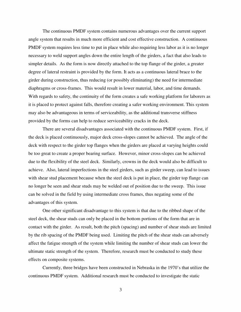
The continuous PMDF system contains numerous advantages over the current support

angle system that results in much more efficient and cost effective construction. A continuous

PMDF system requires less time to put in place while also requiring less labor as it is no longer

necessary to weld support angles down the entire length of the girders, a fact that also leads to

simpler details. As the form is now directly attached to the top flange of the girder, a greater

degree of lateral restraint is provided by the form. It acts as a continuous lateral brace to the

girder during construction, thus reducing (or possibly eliminating) the need for intermediate

diaphragms or cross-frames. This would result in lower material, labor, and time demands.

With regards to safety, the continuity of the form creates a safe working platform for laborers as

it is placed to protect against falls, therefore creating a safer working environment. This system

may also be advantageous in terms of serviceability, as the additional transverse stiffness

provided by the forms can help to reduce serviceability cracks in the deck.

There are several disadvantages associated with the continuous PMDF system. First, if

the deck is placed continuously, major deck cross-slopes cannot be achieved. The angle of the

deck with respect to the girder top flanges when the girders are placed at varying heights could

be too great to create a proper bearing surface. However, minor cross-slopes can be achieved

due to the flexibility of the steel deck. Similarly, crowns in the deck would also be difficult to

achieve. Also, lateral imperfections in the steel girders, such as girder sweep, can lead to issues

with shear stud placement because when the steel deck is put in place, the girder top flange can

no longer be seen and shear studs may be welded out of position due to the sweep. This issue

can be solved in the field by using intermediate cross frames, thus negating some of the

advantages of this system.

One other significant disadvantage to this system is that due to the ribbed shape of the

steel deck, the shear studs can only be placed in the bottom portions of the form that are in

contact with the girder. As result, both the pitch (spacing) and number of shear studs are limited

by the rib spacing of the PMDF being used. Limiting the pitch of the shear studs can adversely

affect the fatigue strength of the system while limiting the number of shear studs can lower the

ultimate static strength of the system. Therefore, research must be conducted to study these

effects on composite systems.

Currently, three bridges have been constructed in Nebraska in the 1970’s that utilize the

continuous PMDF system. Additional research must be conducted to investigate the static

4

strength and fatigue endurance provided as well as lateral bracing requirements before the

benefits of the continuous PMDF system can be fully utilized in the field.

1.2 Objectives and Scope of Study

The objective of this study is to investigate the viability of using continuous steel deck

forms in the design and construction of steel-concrete composite bridges. This research will be

restricted to simple span bridges with rolled wide flange steel girders without significant camber

or cross-slopes. The ultimate goal of the research is to begin to establish proof of concept for

continuous steel deck construction in bridges.

The focus of this document is on three aspects of the continuous steel deck system: the

fatigue endurance, static strength, and lateral bracing provided by the forms during deck

placement. A full scale composite beam test specimen was constructed and tested to investigate

the objectives stated above. The specimen consisted of two simply supported girders with no

intermediate diaphragms or cross frames installed. End diaphragms were used. Steel deck form

was placed continuously across the top flanges with ribs oriented perpendicular to the girders.

Headed shear studs were welded through the deck into the top flange and a concrete deck placed

to create a composite system. The two halves of the specimen were different in that one half

used one stud per rib while the other half used two studs per rib to create two different specimen

types. The adequacy of the steel deck forms as lateral bracing of the girders was investigated by

first determining the required form stiffness using equations derived by Helwig and Yura (2008a,

2008b) followed by an examination of the system behavior during the placement of the concrete

deck. The fatigue endurance of the system was evaluated by subjecting the test specimen to two,

1.2 million cycle fatigue tests while monitoring loss of stiffness over the course of each test. A

fatigue test was conducted on each half of the bridge with loading at the quarter points to

determine the effects that different levels of shear connection have on the fatigue life of the shear

span. Once the fatigue tests were completed, the test specimen was subjected to a linearly

increasing static load until the system stopped taking load to investigate the residual strength of

the continuous form system. Static tests were conducted on each half of the specimen. The goal

of the static testing was to determine if existing design models can properly predict the plastic

moment capacity of this system or if changes must be made.

5

1.3 Organization of Thesis

Chapter two provides a literature review that includes background information for lateral

bracing of beams along with design recommendations for the lateral bracing of steel bridge

girders during concrete deck placement, methods of determining partial interaction behavior of

composite beams in the linear elastic range, the behavior or shear studs under fatigue loading,

and methods of calculating the ultimate strength of composite beams. Chapter three gives details

of the design, instrumentation, and testing of the composite bridge in this study. Chapter four

discusses the results of supplemental tests used to support the specimen testing. Chapter five

provides the results of the two fatigue tests conducted. Chapter six provides the results of the

three static tests conducted. Chapter seven highlights the conclusions reached as result of the

tests conducted on the test specimen and includes comparisons to existing design provisions and

recommendations for future research.

6

Chapter 2: Literature Review

2.1 Lateral Stability of Girders

Lateral stability is very important to consider during the design of steel bridge girders.

This becomes an issue mainly during the construction phase of a steel girder bridge when the

concrete is still fresh, creating a large uniform dead load on the girders while providing no lateral

restraint for the compression flange of the girders. The failure mechanism that results is known

as Lateral-Torsional Buckling. Lateral-torsional buckling (LTB) is a failure mode that involves

both a twist and lateral displacement of the section, as illustrated in Fig. 2.1. It is possible to

prevent such failure by restraining either torsional or lateral deformations (Yura 2001).

u

θ

Figure 2.1: Lateral-torsional buckling

2.1.1 Bracing Introduction

Extensive research has been conducted on the topic of column and beam bracing.

Research was conducted by Winter (1960) to study the effects of bracing on columns. Winter

determined that an effective brace requires both adequate stiffness and sufficient strength, with

the required strength being based on the magnitude of the initial out-of-straightness of the

member being braced as well as the brace stiffness. In this context, the ideal stiffness, βi, is

defined as the stiffness at which buckling is forced to occur between brace points, as shown in

Fig. 2.2 (Yura 2001). It was shown that for a given initial out-of-straightness and a brace with

stiffness equal to the ideal stiffness and located at the mid-height of the column, both the brace

force (Fbr) and the deflection at the brace become very large as the axial load approaches the

7

buckling load. Further results showed that if the stiffness is overdesigned to two or three times

the theoretical ideal stiffness, deflections and brace forces are greatly reduced. This leads to the

conclusion that to be considered effective, braces should be designed for stiffnesses greater than

the ideal stiffness to control brace forces and deflections (Winter 2001).

βb > βi βb < βi

Figure 2.2: Buckling shapes for brace stiffness above and below ideal (adapted from Yura 2001)

Due to the flexure and torsion resulting from the loading of beams, beam bracing

becomes significantly more complicated than column bracing. Research has been conducted by

Yura (2001) where the effects of brace type, load location, brace location, brace stiffness, and

number of braces for beams was investigated using many different elastic finite element

simulations. The study focused on two types of beam bracing, lateral and torsional, with the

understanding that an effective brace resists the twist of the cross-section. Lateral bracing is

defined as a brace that prevents lateral movement of the member it’s bracing, within which there

are four different classifications: relative, discrete, lean-on, and continuous. Torsional bracing is

defined as bracing that directly restrains twist of the cross-section and contains the sub-types

discrete and continuous. The remainder of this section will focus only on lateral continuous

bracing and the factors affecting it as this is the type of bracing utilized in the current study.

Various factors were shown to influence the effectiveness of lateral bracing. The location

of the loading is one such factor. Yura et al. (1992) illustrate that top flange loading is a more

severe case than loading at the centroid or bottom flange. This is because top flange loading

causes a reduction in buckling strength resulting from an increase in twist due to load

eccentricity, while bottom flange loading increases buckling strength due to a restoring force

8

created by load eccentricity. Yura (2001) states that the brace should be placed where it will

offset the twist to the greatest degree, therefore bracing applied at the top flange in simple span

beams subject to top flange loading causing positive moment will be more effective than bracing

placed at the centroid of the section. Top flange loading causes the center of twist to move

towards the centroid, which renders a lateral brace placed at the centroid ineffective because

there will be no appreciable lateral movement at the brace location. If the loading travels to the

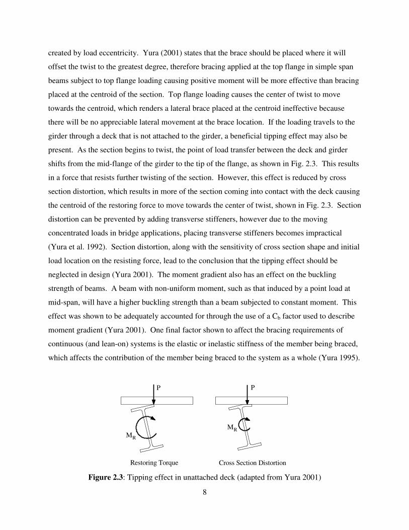
girder through a deck that is not attached to the girder, a beneficial tipping effect may also be

present. As the section begins to twist, the point of load transfer between the deck and girder

shifts from the mid-flange of the girder to the tip of the flange, as shown in Fig. 2.3. This results

in a force that resists further twisting of the section. However, this effect is reduced by cross

section distortion, which results in more of the section coming into contact with the deck causing

the centroid of the restoring force to move towards the center of twist, shown in Fig. 2.3. Section

distortion can be prevented by adding transverse stiffeners, however due to the moving

concentrated loads in bridge applications, placing transverse stiffeners becomes impractical

(Yura et al. 1992). Section distortion, along with the sensitivity of cross section shape and initial

load location on the resisting force, lead to the conclusion that the tipping effect should be

neglected in design (Yura 2001). The moment gradient also has an effect on the buckling

strength of beams. A beam with non-uniform moment, such as that induced by a point load at

mid-span, will have a higher buckling strength than a beam subjected to constant moment. This

effect was shown to be adequately accounted for through the use of a Cb factor used to describe

moment gradient (Yura 2001). One final factor shown to affect the bracing requirements of

continuous (and lean-on) systems is the elastic or inelastic stiffness of the member being braced,

which affects the contribution of the member being braced to the system as a whole (Yura 1995).

Restoring Torque Cross Section Distortion

P

MR

MR

P

Figure 2.3: Tipping effect in unattached deck (adapted from Yura 2001)

9

2.1.2 Steel Girder Bracing Requirements

A type of bracing present in steel girder bridges is continuous bracing provided by the

steel deck (used as concrete formwork) that acts as a shear diaphragm attached to the top flange

of the girder. The steel deck has a large in-plane stiffness that works to resist any lateral twisting

of the top flange caused by loading (Helwig and Yura 2008a) which might lead to lateral-

torsional buckling of the member. In a study conducted by Helwig and Frank (1999) on slender-

web plate girders, it was determined that brace stiffness requirements are a function of the

location of both the load as well at the type of loading. Equation 2.1 was developed to determine

the buckling capacity of a beam braced by a shear diaphragm:

dQmMCM gbcr += * (2.1)

Where: Mcr = moment strength of diaphragm-braced girder

*

bC = moment gradient factor, taking into account load height

= 4.1bC (Helwig et al. 1997)

Mg = moment strength of the girder without bracing

m = load type factor

Q = shear rigidity of diaphragm

d = beam depth

Values of m recommended are 1.0 for loads creating a uniform moment, 0.625 for gravity loads

applied at midheight, and 0.375 for gravity loads applied at the top flange. The shear rigidity, Q,

is the product of the tributary width of the steel deck (sd) and the effective shear modulus, G’,

which can be calculated for a given deck by using equations present in Steel Desk Institute

Diaphragm Design Manual (Luttrell 2004).

An effective brace requires both adequate stiffness and strength. The research of Helwig

and Frank (1999) was continued to study the strength and stiffness requirements of diaphragm-

braced beams by (Helwig and Yura 2008a and 2008b). They conducted finite element analyses,

using the program ANSYS, of multiple section sizes evaluating the effects of load location, brace

stiffness, section slenderness, girder span-to-depth ratios, and the presence of intermediate

braces. The results were used to produce design equations to determine strength and stiffness

requirements of shear diaphragm-braced bridge girders. The results presented were those for a

W16x26 section, which has one of the most slender webs available for rolled shapes and

10

therefore results presented are typically conservative if a section with a stockier web is used

(Helwig and Yura 2008b). A new definition of “ideal stiffness” was presented due to the fact

that there is no unbraced length in continuous bracing. Ideal stiffness is now defined as the brace

stiffness required to reach a predetermined load on a perfectly straight beam, and this ideal value

was calculated from an Eigen value buckling analysis of the section. For the study, an initial

imperfection of dL 500θ0 = was chosen, where 0θ is the initial angle of imperfection with

respect to the vertical, L is the span length, and d is the depth of the steel section. This is twice

the value used in building design based on the fact that unlevel bearing surfaces for the bridge

girders can lead to larger initial imperfections (Helwig and Yura 2008a). Results of the study

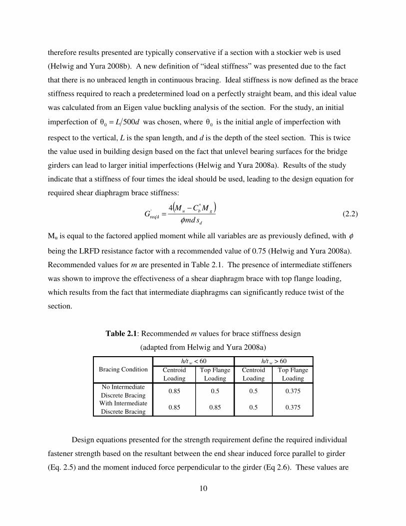
indicate that a stiffness of four times the ideal should be used, leading to the design equation for

required shear diaphragm brace stiffness:

( )d

gbu

sdm

MCMG

φ

*

'

dreq'

4 −= (2.2)

Mu is equal to the factored applied moment while all variables are as previously defined, with φ

being the LRFD resistance factor with a recommended value of 0.75 (Helwig and Yura 2008a).

Recommended values for m are presented in Table 2.1. The presence of intermediate stiffeners

was shown to improve the effectiveness of a shear diaphragm brace with top flange loading,

which results from the fact that intermediate diaphragms can significantly reduce twist of the

section.

Table 2.1: Recommended m values for brace stiffness design

(adapted from Helwig and Yura 2008a)

No Intermediate

Discrete Bracing

With Intermediate

Discrete Bracing0.3750.50.850.85

0.3750.50.50.85

Bracing Condition

h/t w < 60 h/t w > 60

Centroid

Loading

Top Flange

Loading

Centroid

Loading

Top Flange

Loading

Design equations presented for the strength requirement define the required individual

fastener strength based on the resultant between the end shear induced force parallel to girder

(Eq. 2.5) and the moment induced force perpendicular to the girder (Eq 2.6). These values are

11

based on the brace moment per unit length, '

brM (Eq 2.4), which includes a correction factor for

overdesigning the diaphragm stiffness, Cr (Eq 2.3):

+=

'

'

'

4

1

4

3

prov

dreq

rG

GC (2.3)

2

' 001.0d

CLMM ru

br = (2.4)

M

brM

x

MF

'

= (2.5)

ed

dbr

VVnL

wMxF

'

= (2.6)

( ) ( )22

MVR FFF += (2.7)

Where: Cr = brace force reduction coefficient

'

brM = brace moment per unit beam length

Mu = maximum girder design moment between discrete brace points

L = total span of girder

d = distance between girder flange centroids

xM = moment force adjustment factor based on number of fasters, see Table 2.2

xV = shear force adjustment factor based on number of fasters, see Table 2.2

wd = width of diaphragm sheet

ne = number of fasteners per panel at end of diaphragm sheet

FM = component of brace force perpendicular to girder longitudinal axis

FV = component of brace force perpendicular to girder longitudinal axis

FR = resultant force in end fastener

The resultant force is then the force that an individual diaphragm end fastener has to be able to

resist (Helwig and Yura 2008b).

12

Table 2.2: Adjustment factors for strength design (adapted from Helwig and Yura 2008b)

n e x V x M

2 1.00 1.000

3 1.00 0.667

4 1.11 0.500

5 1.25 0.400

6 1.38 0.333

2.1.3 AASHTO LRFD Requirements

Current AASHTO LRFD (2007) specifications state that it is incorrect to assume that

metal stay-in-place deck forms (steel deck) will provide adequate lateral stability to the top

flange in compression during the curing of the deck. This requirement assumes that the steel

deck is not continuous over the girders. Lateral torsional buckling of bridge girders is controlled

through the use of intermediate diaphragms or cross-frames. The specifications provide limits to

the unbraced length (or spacing) that can be utilized when placing these braces, as given in Eq

2.8:

10RLL rb ≤≤ (2.8)

Where: Lb = spacing of intermediate diaphragms or cross-frames (ft.)

Lr = limiting unbraced length (ft.)

R = minimum girder radius within the panel (ft.)

The R/10 limit is applicable only in horizontally curved I-girder bridges as well as an upper

bound of 30.0 ft. on Lb and will be ignored for the remainder of the section. The limiting

unbraced length, Lr, is defined as the maximum length required to achieve nominal yielding in

either flange under uniform bending while taking into account pre-existing residual compressive

stress effects in the flange, which is the non-compact bracing limit given in Eq 2.9 in which

inelastic buckling will occur:

yr

trF

ErL π= (2.9)

Where: rt = effective radius of gyration of gyration for lateral torsional buckling (in.)

E = modulus of elasticity of steel section (ksi)

13

Fyr = compression flange stress at the onset of nominal yielding, taking into

account residual stress effects but not including compression flange lateral

bending (ksi); it is the smaller of 0.7Fyc or Fyw, but greater than 0.5Fyc

Fyc = yield stress of the compression flange steel (ksi)

Fyw = yield stress of the steel section web (ksi)

2.2 Partial Shear Connection under Service Loading

The usual design practice for composite bridge girders is to design for full interaction

between the steel member and concrete slab. However, for the test setup of this project,

limitations on the number of shear studs that can be used are incurred based on the placement of

the steel deck form on the top flange of the girder and the resulting voids present in ribbing.

Therefore a partial interaction analysis must be performed. In building applications partial

interaction design is frequently used. Partial interaction design is typically more economical

than a full interaction design because a large decrease in the number of shear studs will often

lead to a small decrease in flexural strength.

2.2.1 Partial Interaction Theory

In design it is usually assumed that there is no slip at the steel-concrete interface for fully

composite beams. In reality, however, slip occurs at service load levels due to local crushing of

the concrete around the lower shank of the shear stud and also due to bending of the shear

connector (Kwon et al. 2007). This leads to a partial-interaction state in the composite beam

even though the connector strength assumed to be sufficient for full composite action. Test

results provided by McGarraugh and Baldwin (1971) showed that beams designed for full

composite action had measured stiffnesses of 80 to 90 percent of their calculated values at

service load levels. Models for these beams can be created based on linear elastic partial-

interaction theory. Johnson and May (1975) stated that even though a beam with a partial

connection of greater than 50 percent is less stiff than a beam that is fully composite, it is

acceptable to use linear elastic partial-interaction theory to estimate composite beam behavior in

beams with partial shear connection and that the loading on the beam at the serviceability limit

state is equal to half that required to reach the ultimate moment.

14

In a linear partial-interaction analysis, a governing differential equation is created based

on equilibrium, compatibility, and elasticity that is dependent on the loading condition and

solved using the boundary conditions (Johnson 1995). This review will be limited to the case of

a simply-supported beam with a point loading at a variable location as this is the setup being

investigated in this project’s tests. This review presents an analysis method introduced by

Johnson (1981) for the beam being considered in Fig. 2.4. In this analysis, it is assumed that the

concrete is uncracked and unreinforced, that there is equal curvature in both the concrete slab

and steel member, that shear connectors of the same linear stiffness are placed evenly across the

whole length of the beam, and that loading is low enough to cause a linear load-slip relation

(which should be valid at service loads). Definitions of cross section properties are given in

Fig.2.5a while definitions of internal forces are given in Fig. 2.5b.

W

L

lW 2

x

A C

L

lW 1

1l 2l

L

B

Figure 2.4: Analysis simply-supported beam with point load (adapted from Johnson 1981)

15

x

dxdx

dss +

dx

cy

cd

sy

cc I,A

ss I,A

sM

F

F

q dx

cM

ps

a) Cross section b) Internal forces

sV

cV

Figure 2.5: Variables used for linear partial-interaction analysis (adapted from Johnson 1981)

The governing second order non-homogenous differential equation for the general system

is given by Eq 2.10 (Johnson 1994):

)(2

2

2

Vwxsdx

sd+−=− αβα (2.10)

Where: s = slip at interface

α = property of cross-section = 0IpE

Ak

s

β = property of cross-section = Ak

pdc

0I = transformed moment of inertia of cross-section = ( ) s

c Im

I+

+φ1

A = transformed area of cross-section = ( )

sc

cA

I

A

mId 002 1

++

+φ

m = modular ratio = Es/Ec

k = linear stiffness of shear connectors

w = uniformly distributed load (if any)

V = vertical shear due to a point load (if any)

φ = ratio of creep strain to the elastic strain in concrete at the time considered

16

The variables Ic, Is, Ac, As, dc, and p are as defined in Fig. 2.5. Solving Eq 2.10 for the particular

and complimentary solutions produces the result:

( )VwxxKxKs +++= βαα coshsinh 21 (2.11)

where K1 and K2 are both constants of integration and all other variables are as defined above.

At this point the load and boundary conditions specific to the problem at hand are applied to

solve for the two constants of integration. For the setup involving the point load as shown in Fig.

2.5 the boundary conditions are 0=dx

ds at x = 0 and x = L. Due to the discontinuity in the

moment at the point load, Eq 2.11 must be applied to both spans AB and BC, and therefore four

constants of integration need to be solved for, which is accomplished by taking into account the

continuity of s and dx

ds at x = l1. The final solution for the value of the slip along portion AB of

the span is:

−= 1

sinh

coshsinh4 212

LL

xll

L

lWs

α

ααβ (2.12)

Using this equation for slip, values of the horizontal shear force, increases in curvature and

stress, and deflections can be determined for sections along the composite girder (Johnson 1981).

2.2.2 Applications

Johnson and May (1975) concluded that a full partial-interaction analysis was too

complex to be used for everyday design and established simplified design rules based on existing

data and a parametric study conducted. An equation was presented by Johnson and May that

allowed for the calculation of a conservative estimate for the ultimate moment in a composite

beam with partial shear connection based on results provided from the study of McGarraugh and

Baldwin (1971). It is given as:

( )sf

f

sp MMN

NMM −+= (2.13)

Where: Mp = ultimate moment with partial shear connection

Ms = ultimate moment of the steel section alone

Mf = ultimate moment with full shear connection

N = actual number of shear connectors provided in the shear span

17

Nf = number of shear connectors required for full interaction in the shear span

It is recommended that the above equation only be used for shear connection ratios of 50 percent

or greater because tests show that interface slip increases rapidly at lower connection ratios. This

can lead to lower ultimate moments making the equation less conservative. Johnson and May

(1975) also provided an estimate of the deflections of a composite member with partial shear

connection under service loading, as given by:

( )

−−+=

f

fsfpN

N1δδαδδ (2.14)

Where: pδ = deflection of section with partial shear connection

fδ = deflection of section with full shear connection

sδ = deflection of steel section alone

α = correlation factor

N and Nf are as previously defined. A value of α = 0.5 was recommended for design by the

authors; however, Oehlers and Bradford (1995) provided a lower value of 0.4 in later work.

Other important conclusions presented were that the largest relative change in deflection from

partial interaction resulted from members with high concrete strength, low steel strength, low

connector modulus, strong connectors (resulting in increased connector spacing), a low ratio of

steel to concrete area, and a low span-to-depth ratio (Johnson and May 1975).

Grant et al. (1977) conducted research into composite beams built using formed steel

decking. The goal was to investigate the effects of welding shear connectors through formed

steel deck on connector capacity, flexural capacity, and the behavior of composite beams. The

results were compared to test specimens constructed without formed steel deck as well as

existing design criteria. This was accomplished through the casting and testing of 17 composite

beams with varying steel yield strengths, geometry of steel deck forms, and degree of partial

interaction. Results from 58 previous beam tests were also used in the study. The authors state

that connector forces, beam deflections, and stresses in the concrete slab and steel beams are all a

function of the horizontal forces transferred between the slab and the girder, F. This value is

maximum at full interaction when there is no slip and reduces as slip increases, reaching a point

where F = 0 when there is no shear connection between the beam and slab. Using linear elastic

partial interaction theory, it was concluded that a general relationship could be established

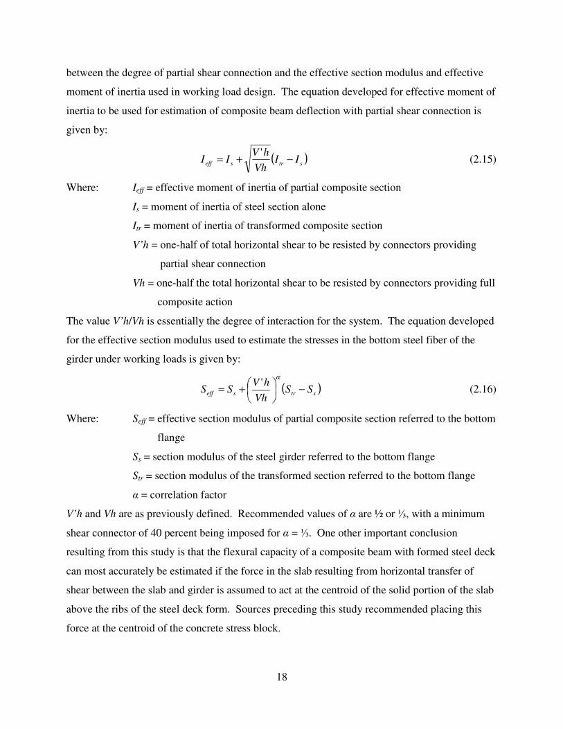
18

between the degree of partial shear connection and the effective section modulus and effective

moment of inertia used in working load design. The equation developed for effective moment of

inertia to be used for estimation of composite beam deflection with partial shear connection is

given by:

( )strseff IIVh

hVII −+=

' (2.15)

Where: Ieff = effective moment of inertia of partial composite section

Is = moment of inertia of steel section alone

Itr = moment of inertia of transformed composite section

V’h = one-half of total horizontal shear to be resisted by connectors providing

partial shear connection

Vh = one-half the total horizontal shear to be resisted by connectors providing full

composite action

The value V’h/Vh is essentially the degree of interaction for the system. The equation developed

for the effective section modulus used to estimate the stresses in the bottom steel fiber of the

girder under working loads is given by:

( )strseff SSVh

hVSS −

+=

α'

(2.16)

Where: Seff = effective section modulus of partial composite section referred to the bottom

flange

Ss = section modulus of the steel girder referred to the bottom flange

Str = section modulus of the transformed section referred to the bottom flange

α = correlation factor

V’h and Vh are as previously defined. Recommended values of α are ½ or ⅓, with a minimum

shear connector of 40 percent being imposed for α = ⅓. One other important conclusion

resulting from this study is that the flexural capacity of a composite beam with formed steel deck

can most accurately be estimated if the force in the slab resulting from horizontal transfer of

shear between the slab and girder is assumed to act at the centroid of the solid portion of the slab

above the ribs of the steel deck form. Sources preceding this study recommended placing this

force at the centroid of the concrete stress block.

19

Current AISC commentary provisions (2005) for the estimation of partial composite

section properties are based on the research of Grant et al. (1977), with slightly different

notation. The equation used for calculation of the effective moment of inertia is given as:

( )str

f

n

seff IIC

QII −

+=

∑ (2.17)

Where: Ieff = effective moment of inertia of partial composite section (in.4)

Is = moment of inertia for the structural steel section (in.4)

Itr = moment of inertia for the fully composite uncracked transformed section

(in.4)

∑ nQ = strength of the shear connectors between the point of maximum positive

moment and the point of zero moment to either side (kips)

Cf = compression force in the concrete slab for fully composite beam; smaller of

ys FA and cc Af'85.0 (kips)

As = area of structural steel section (in.2)

Fy= yield stress of structural steel section (ksi)

'

cf = compressive strength of concrete slab (ksi)

Ac = area of concrete slab within the effective width (in.2)

It is recommend is the commentary that the value of the effective moment of inertia used in

design is to be reduced to 0.75 Ieff . Similarly, the equation for the section modulus of the partial

composite section is given as:

( )str

f

n

seff SSC

QSS −

+=

∑ (2.18)

Where: Seff = effective section modulus of partial composite section referred to the bottom

flange

Ss = section modulus for the structural steel section, referred to the tension flange,

(in.3)

Str = section modulus for the fully composite uncracked transformed section,

referred to the tension flange of the steel section (in.3)

All other variables are as defined previously.

20

A study was conducted into the behavior of post-installed shear connectors used to

increase the capacity of existing non-composite bridge girders in which partial interaction was

used (Kwon et al. 2007). Five full-scale non-composite beams, all simply-supported, were

constructed and four were retrofitted with post-installed shear connectors while the fifth was left

non-composite to act as a reference model. Because of the large expense involved with installing

post-installed shear connectors, a lesser number of connectors were used in the tests than would

be required for full interaction to simulate real-world limitations. The stiffness of the member

was investigated in tests by measuring applied load, vertical deflection at quarter points and

midspan, slip at quarter points and end, and longitudinal strain to track the neutral axis. Also, the

effect of connector placement resulting from the partial shear connection was investigated using

finite element models as well as the results of previous studies. Analysis and test results show

that concentration of shear connectors near supports (points of zero moment) as opposed to

uniformly spacing the connectors led to a decrease in end slip. This helped to redistribute the

load among the shear connectors, thus increasing the deformation capacity of the girder. It was

concluded the post-installed shear connectors are an effective method of improving existing

bridges, as 30 to 50 percent of the studs required for full connection can be used to achieve a 40

to 50 percent increase in capacity of the bridge girders.


Current AASHTO LRFD (2007) specifications do not allow for the partial composite

design of bridge girders. Shear connectors are first designed (in terms of size, number, and

pitch) to meet the fatigue limit state. From there, the ultimate strength of the composite system

is checked assuming full-interaction between the concrete slab and steel girder. This assumes

that the number of shear studs is adequate to fully transfer the longitudinal shear force between

the two components which is equal to the lesser of the force required to fully yield the steel

section or the force to cause the concrete slab to reach its full compressive capacity. The number

of shear connectors is usually controlled by fatigue requirements and therefore most new bridges

being designed have full composite interaction.

21

2.3 Fatigue Requirements

2.3.1 Fatigue of Shear Connectors

The behavior of shear connectors under fatigue loading was studied extensively by

Slutter and Fisher (1967) and this work is the basis for the current AASHTO-LRFD

specifications. In this landmark study, fatigue tests to failure of 56 push-out specimens were

conducted to investigate the effects of stress range and minimum stress level in the connectors on

the number of cycles before failure in the beam. Three types of shear connectors were tested: 35

specimens using ¾ in. stud connectors, 9 specimens using ⅞ in. stud connectors, and 12

specimens using 4-inch, 5.4 lb channel connectors. The remainder of this review will focus on

the stud connectors only. Specimens were tested using a factorial combination of five maximum

stresses, five stress ranges, and three levels of minimum stress with three specimens being tested

at each combination for the ¾ in. stud connectors and one specimen for each combination for the

⅞ in. stud connectors. A few important conclusions were drawn from this data; there are no

significant differences in fatigue life between the ¾ in. and ⅞ in. stud connectors, there was no

leveling off of the S-N curves produced, the specimens with stress reversal resulted in longer

fatigue life, and the minimum stress level had a very minimal effect on fatigue life. Therefore,

the stress range was determined to be the most significant variable. A design equation was fit to

the data using linear regression, ignoring the stress reversal results, as given by:

rSN 1753.0072.8log −= (2.19)

Where: N = number of cycles to failure of a shear connector

Sr = range of shear stress (ksi)

This equation can then be used to determine the allowable range of shear force per stud using

Equation 2.18:

2

sr dZ α= (2.20)

Where: Zr = allowable range of shear force per stud (lbs)

α = constant based on number of cycles in the life of the structure

2

sd = diameter of the stud (in)

The equations above are applicable to both ¾ in. and ⅞ in. stud connectors and are conservative

for connectors of smaller diameter. The authors also give design methods for calculating

connector spacing based on fatigue considerations and methods for fulfilling flexibility

22

requirements. It was also shown that concrete strength did not significantly affect the fatigue

lives of the connectors.

Oehlers and Foley (1985) also researched the fatigue life (number of cycles) of headed

shear studs in composite beams. The study focused on fatigue crack propagation through the

shank of the stud over the fatigue life. The failure point was determined using data from eleven

new push tests, 118 existing push test results, and a computer analysis. It was shown that cracks

are present as result of the welding process and these cracks begin to spread through the shank of

the shear connector as soon as cyclic load begins. The rate at which the crack propagates

through the shank is assumed to be constant over the fatigue life as long as the shear range

remains constant, with the shear range being that which causes tension on one side of the stud.

The shear stud fractures once the strength of the uncracked area of the shank is less than the peak

of the cyclic load, called a “fast fracture,” with the strength being directly proportional to the

uncracked area. The main conclusion drawn here is that the static strength of shear studs begins

to decrease as soon as cyclic loads are applied. Based on these results, two equations were

produced to predict fatigue life: Eq 2.21 gives the fatigue life assuming that the fatigue crack

can completely pass through the shank without fracture occurring while Eq 2.22 gives the fatigue

life including fracture but not including peak load effects.

−=

sh

tf

P

RN 1010 log55.437.3log (2.21)

−=

sh

tf

P

RN 1010 log95.492.2log (2.22)

Where: Nf = fatigue life assuming full crack propagation

Ne = fatigue life with shank fracture not including peak load

Rt = tensile range of cyclic shear load

Psh = calculated stud static failure load

Oehlers et al. (2000) conducted research into the beneficial effects of friction at the steel-

concrete interface on the fatigue endurance of headed shear studs in composite bridge beams.

The goal of this research was to determine what effect interface shear had on shear stud life and

to produce an equation for simple analysis of the remaining life of both new and existing

composite girders considering friction. This was accomplished using a finite element model with

linear elastic properties subjected to different fatigue load patterns, including a static point load,

23

a single moving point load, and single fatigue vehicle consisting of two point loads to determine

values for the total longitudinal shear and the friction force at the interface. Once these values

were known, they were applied to fatigue equations to produce the final hand assessment

equation. It was shown that taking interfacial friction into account can lead to a large increase in

the fatigue life of stud connectors. This is due to the fact that part of the shear forces being

transferred between the steel element and concrete slab can be transmitted through friction which

in turn reduces the amount of shear that is taken by the shear connectors themselves thus

reducing the stress range applied to the connectors and increasing the fatigue life. The hand

equation produced is:

∑=

=

−

−

=kz

z

ff

st

res

st

FLT

Q

Q

Q

1

12.3

1.5

101

(2.23)

Where: Qst = static shear flow strength of shear stud

Qres = remaining shear flow strength of connector after cycling

T = number of fatigue vehicles that have travelled over the bridge

Lf = load constant

Ff = force constant

The load constant and force constant are based on the number and type of different fatigue

vehicles that will travel over the bridge and their relative frequencies.


AASHTO LRFD (2007) specifications are based on the work of Slutter and Fisher (1967)

with some slight modifications. The fatigue shear resistance, in kips, of an individual shear

connector for a specified number of loading cycles is given by:

2

5.5 22 d

dZr ≥= α (2.24)

Where: Zr = fatigue shear resistance of an individual shear connector (kips)

α = Nlog28.45.34 −

d = diameter of shear connector shank (in)

N = number of loading cycles in the structure life

24

Once the fatigue shear resistance has been determined, the horizontal fatigue shear range per unit

length must be determined. Note that what is important is the shear range, not the maximum

shear force in these calculations, as given by:

( ) ( )22

fatfatsr FVV += (2.25)

Where: Vsr = horizontal fatigue shear range per unit length (kip/in)

Vfat = longitudinal shear force per unit length = I

QV f

Ffat = radial fatigue shear range per unit length (kip/in)

Vf = vertical shear force range under the fatigue load (kips)

The value for Ffat is taken as zero in non-curved girders. Once the range of horizontal shear is

known, the pitch (spacing) of the shear connectors is determined using Eq 2.26:

sr

r

V

nZp ≤ (2.26)

Where: p = pitch of shear connector groups (in)

Zr = fatigue shear resistance of an individual shear connector (kips)

Vsr = horizontal fatigue shear range per unit length (kip/in)

n = number of shear connectors per group

The resulting distribution of shear connectors does not have to be uniform along the length of the

beam as the pitch depends on the horizontal shear range, which itself can vary along the length of

the beam. When more than one shear connector is going to be used per group, the connectors are

not allowed to be placed less than 4.0 stud diameters center-to-center and a clear distance of 1.0

inch is required between the end of the flange and the connector.

2.4 Static Strength of Composite Beams

2.4.1 Static Strength of Shear Connectors

This section investigates different methods of calculating the static strength of headed

shear connectors (shear studs) embedded in a concrete deck. The AASHTO LRFD (2007)

specifications provide a method for calculating this value based on the work of Ollgaard et al.

(1971) as given by:

uscccscn FAEfAQ ≤= '5.0 (2.27)

25

Where: Asc = cross-sectional area of shear connector (in2)

'

cf = rib concrete compressive strength (ksi)

Ec = modulus of elasticity of concrete (ksi)

Fu = specified minimum tensile strength of a shear stud (ksi)

The above equation only applies to solid slab construction, with the concrete deck cast directly

against the steel girder top flange.

When profiled sheeting is used as formwork, modifications to the above values are

required. According to Johnson (1995), when considering materials of the same strength, shear

connectors placed in the ribs of decks cast using profiled sheeting sometimes have a lower shear

resistance compared to those cast in a solid slab. This is caused by local failure of concrete in

the ribs. It is recommended that reduction factors be applied to the shear resistance of the shear

connectors calculated for solid slab construction. The reduction factor varies based on whether

the ribbing is oriented parallel or perpendicular to the longitudinal axis of the girders. Only the

case of ribs oriented perpendicular to the girders will be investigated in this thesis. The value of

the reduction factor, kt, as given by Johnson is:

0.117.0

≤

−=

pp

o

r

th

h

h

b

Nk (2.28)

Where: bo = width of rib taken at the centroidal axis of the profiled steel sheeting

Nr = number of shear connectors in one rib, not to exceed 2 in calculations

hp = distance from top of slab to centroidal axis of profiled steel sheeting

h = height of shear connector

The equation above was based on equations developed in North America; however they have

been modified to fit European deck profiles. Also, there is no distinction provided in Eq 2.28

between shear connectors welded through the steel deck form and those welded through a hole in

the form (Johnson 1995).

Easterling et al. (1993) conducted a study that investigated the strength of shear studs in

composite beams when profiled steel deck form is used. The focus of this study was on the

placement of the shear stud within that rib, with the shear stud being in either a “strong” or

“weak” position. The need for this distinction results from the fact that shear studs have to be

placed off center due to the presence of a stiffener rib that runs down the center of the bottom

flange of the steel deck. A shear stud is said to be in the “weak” position if it is placed on the

26

side of the deck stiffener closest to the end of the span as opposed to a shear stud in the “strong”

position which is placed on the side of the deck stiffener closest to the point of maximum

moment, as shown in Fig. 2.6. Differences in strength had been noted between the strength of

the shear studs in either position, a fact which is partially explained by the amount of concrete

between the shear stud and the deck web (Easterling et al. 1993). From the results of four

composite beam tests and eight push-out tests, Easterling et al. showed that existing design

methods for calculating the static strength of shear studs were unconservative, with shear studs

placed in the weak position having a lower static strength than those placed in the strong

position. In the beam tests, shear studs in the strong position tests failed by either shearing of the

stud shank or by the formation of a concrete shear cone. In the push-out tests, studs failed by the

formation of a failure surface in the concrete. Therefore, it was determined that stud strength as

a function of the concrete strength. Weak side studs failed by punching through the web of the

steel deck without developing the full strength of the concrete or stud shank, therefore the shear

stud strength was taken as a function of the steel deck strength. Easterling et al. made no

recommendations for changes to existing standards in this study.

Deck Stiffener

HorizontalShear Force

Strong SideWeak Side

Figure 2.6: Strong Side versus Weak Side shear stud placement

(adapted from Easterling et al.1993)

Research conducted by Rambo-Roddenberry (2002) at Virginia Tech investigated the

strength of welded shear stud connectors in composite beams. The effects of friction, stud

position in the rib, normal force, concrete strength, and stud properties on shear stud strength

were studied through the testing of twenty-four solid slab push-out tests, 93 composite slab push-

27

out tests, and bare studs. Also, the effects of shear stud diameter, steel deck height, and the

number of studs on stud strength were examined. Specimens utilizing profiled steel deck were

constructed with the ribs oriented perpendicular to the beams. The goal of this research was to

produce a new stud strength prediction model that accurately takes into account all of the design

variables mentioned previously. This model was then verified using the above tests and the

results of 61 other beam tests that had been reported previous to this research. The stud strength

prediction equation produced for shear studs in 2 in. and 3 in. deck with a stud diameter to flange

thickness ratio of less than or equal to 2.7 that is applicable to this research is given in Eq 2.29.

usdnpsc FARRRQ = (2.29)

Where: Rp = 0.68 for emid-ht. ≥ 2.2” (strong position studs)

= 0.48 for emid-ht. ≤ 2.2” (weak position studs)

= 0.52 for staggered position studs

Rn = 1.0 for one stud per rib or staggered

= 0.85 for two studs per rib

Rp = 1.0 for all strong position studs

= 0.88 for 22 gage deck (weak studs)




The AISC Specification for Structural Steel Buildings (2005) provides a method of

calculating the static strength of shear studs that takes into account the effects of placement in the

steel deck form ribs that is based on the work by Rambo-Rodenberry (2002). The equation for

calculating the static strength of a shear connector as provided by the AISC Specification (2005)

is given by:

uscpgccscn FARREfAQ ≤= '5.0 (2.30)

Where: Asc = cross-sectional area of shear connector (in2)

'

cf = rib concrete compressive strength (ksi)

Ec = modulus of elasticity of concrete (ksi) = '5.1

cc fw

wc = unit weight of concrete

Fu = specified minimum tensile strength of a shear stud (ksi)

28

Rg = 1.0 for one stud welded in a steel deck rib

= 0.85 for two studs welded in a steel deck rib

= 0.7 for three or more studs welded in a steel deck rib

Rp = 0.75 when 0.2≥−htmide in.

= 0.60 when 0.2<−htmide in.

htmide − = the distance from the edge of the stud shank to the steel deck web measured

at the mid-height of the deck rib and in the load-bearing direction (toward

the point of maximum moment)

The values given above correspond only to profiled steel deck with ribs oriented perpendicular to

the steel shape with shear studs welded through the steel deck into the steel shape. Eq 2.30 is the

same as the AASHTO LRFD (2007) equation (2.27) except for the addition of the Rg term that

accounts for the number of studs in a rib and he Rp term that accounts for weak or strong side

shear stud placement.

29

Chapter 3: Design, Fabrication, and Testing

3.1 Girder Design and Fabrication

3.1.1 Introduction

This section provides the details of the girder design, steel frame fabrication, and girder

instrumentation for the specimen constructed and tested. This section does not include the

details of the composite section design as that will be covered in a separate section to follow.

Details of the design include determination of girder size, bearing stiffener design and details,

and end diaphragm design and details. This is followed by discussions of the fabrication of the

test specimen and of the specifics of the instrumentation utilized.

3.1.2 Girder Design and Details

The girders used in this project have been designed as typical interior girders of the

fictitious design bridge shown in Fig. 3.1. The bridge was designed as simply supported with a

span of 30 ft. This span was chosen because it represents a typical span length for bridges in

which this design system is intended in the field as well as being a length which can easily be

accommodated in the lab. The design of the bridge superstructure was conducted following the

2007 AASHTO LRFD Bridge Design Specifications with the only departures occurring in the

areas covered by the scope of this project, as will be described in later sections of this chapter.

46' - 6"

6 @ 7' - 0" = 42' - 0"

Barrier18"

2.5" Stay-in-PlaceForm

8"Deck

Figure 3.1: Full design bridge cross-section

30

The details of the design are provided in Appendix A. A two interior girder section of the bridge

(with effective deck flanges) was constructed and tested at full scale. The girders used in the

design and test specimen were W21x50 sections composed of A992 steel with the section

properties provided in Table 3.1. Several other sections were considered for use (W21x55,

W21x62, W24x55, W24x62, and W24x68) however the W21x50 section was chosen because it

was the most economical section that fulfilled the requirements of the design bridge. The girders

have a total length 32 ft to allow for the full bearing area of the neoprene bearing pads to be used

as well as for ease of detailing.

Table 3.1: W21x50 section properties

Depth 20.8 in

Area 14.7 in2

tw 0.380 in.

bf 6.53 in.

tf 0.535 in.

Ix984 in

4

Sx94.5 in

3

W21x50 Section Properties

As result of the large loads at the bearings due to self-weight of the test specimen and the

fatigue and static loads applied, the girder web alone was not thick enough to satisfy the Strength

limit state provisions for Web Yielding and Web Buckling and therefore, bearing stiffeners were

added. The bearing stiffeners also provided a way for the end diaphragms to be framed into the

girders and therefore the stiffeners on the interior girder face were detailed keeping this in mind.

The details for the stiffeners are provided in Fig. 3.2. The stiffeners have a thickness of 3/8 in.

The stiffeners were welded to the top flange, web, and bottom flange at the center of bearing

locations before installation of strain gauges so that the welding process did not damage the

gauges. No intermediate stiffeners were used as the loading is through the deck and therefore

does not act as a point load. Also, as part of the scope of this project, no intermediate

diaphragms or cross frames were used because it is assumed that adequate lateral bracing is

provided by the steel deck. This goes against AASHTO LRFD (2007) specifications which state

that steel deck should not be assumed to provide sufficient lateral support to the girder top flange

31

during deck placement. Therefore, no intermediate stiffeners were required for framing

purposes.

1.25" 1.75"

1.75"4"

3"

3"19.75"

1.5"

13/16"Diameter

Figure 3.2: Bearing stiffener details

End diaphragms are required to add stability to the girders during framing and also to

transfer wind load from the concrete deck to the bearings in the design bridge. The end

diaphragms were designed as compression members and detailed according to AASHTO LRFD

(2007) specifications, which require that end diaphragms be greater than one-half the depth of

the steel girders. The lightest member allowed under this specification was a C12x20.7, which

had more than enough compressive capacity and therefore was chosen for use in the test

specimen. Details of the diaphragm member are given in Fig. 3.3. The final steel frame system

(girders, stiffeners, and diaphragms) is shown in Fig. 3.4.

6' - 10 5/8"

3"

3"

3"

3"

1 1/4"

13/16" Diameter

Figure 3.3: End diaphragm detail

32

C12x20.7End Diaphragm

7' - 0"GirderSpacing

30' - 0"Center of Bearing to Center of Bearing

NeopreneBearing Pad

Bearing Stiffener

32' - 0"Total Girder Length

W21x50 Girders

PLAN

ELEVATION

Girder 2 (G2)

Girder 1 (G1)

FA

R

NE

AR

Figure 3.4: Final steel frame system

3.1.3 Girder Fabrication and Materials

All of the steel sections for the test specimen were fabricated in the Virginia Tech

Structures Laboratory where the test specimen was constructed and tested. The W21x50

members had been cut to the specified 32 ft length by the steel supplier, with the 3 ft drops

included for material property testing, and therefore no additional modifications were required.

No girder camber was requested from the steel supplier. Both the bearing stiffeners and end

diaphragms were fabricated in the lab. The bearing stiffeners were welded in place first and then

girders were set at the required 7 ft spacing. Once the girders were in place, end diaphragms

were installed and then any skew in the frame was removed by checking that both diagonals of

the steel frame were equal and adjusted if necessary. Coupons were cut from the girder drops

and tensile tests were conducted to determine girder steel properties. After the steel framing

system had been put in place, it was discovered that Girder 1 (G1) had a slight (~.75”) lateral

sweep at midspan, a fact that could affect clear edge distances for the shear studs with respect to

the girder top flange. To solve this, girder ends were secured using C-clamps at bearing

locations (see Fig. 3.2) and a come-along jack was hooked to the bottom flange of the girder and

then secured to the reaction floor. The sweep was then eliminated by jacking the bottom flange

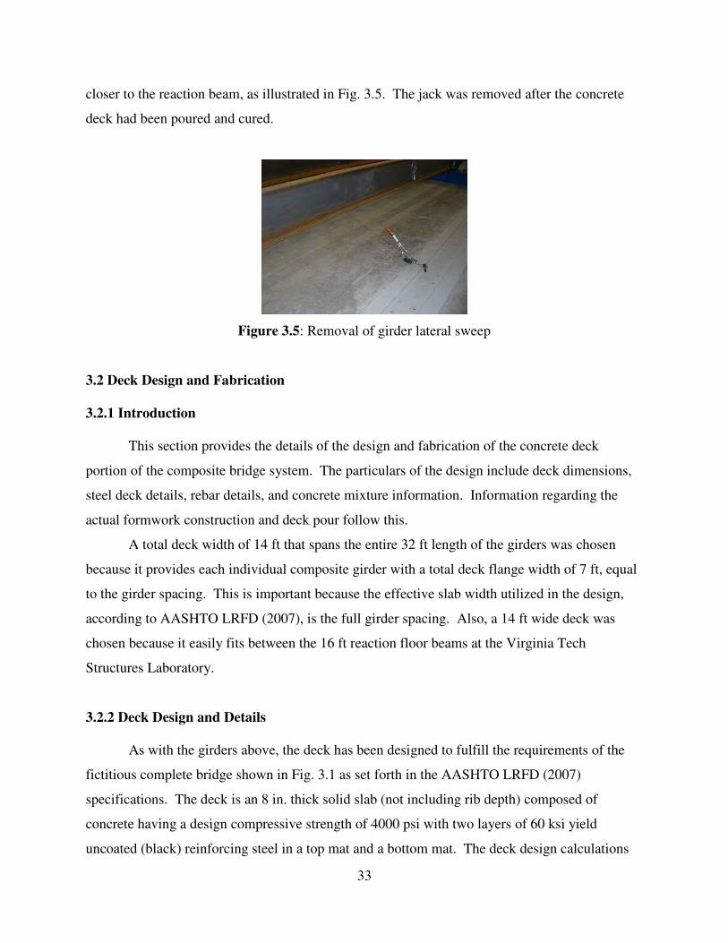
33

closer to the reaction beam, as illustrated in Fig. 3.5. The jack was removed after the concrete

deck had been poured and cured.

Figure 3.5: Removal of girder lateral sweep

3.2 Deck Design and Fabrication

3.2.1 Introduction

This section provides the details of the design and fabrication of the concrete deck

portion of the composite bridge system. The particulars of the design include deck dimensions,

steel deck details, rebar details, and concrete mixture information. Information regarding the

actual formwork construction and deck pour follow this.

A total deck width of 14 ft that spans the entire 32 ft length of the girders was chosen

because it provides each individual composite girder with a total deck flange width of 7 ft, equal

to the girder spacing. This is important because the effective slab width utilized in the design,

according to AASHTO LRFD (2007), is the full girder spacing. Also, a 14 ft wide deck was

chosen because it easily fits between the 16 ft reaction floor beams at the Virginia Tech

Structures Laboratory.

3.2.2 Deck Design and Details

As with the girders above, the deck has been designed to fulfill the requirements of the

fictitious complete bridge shown in Fig. 3.1 as set forth in the AASHTO LRFD (2007)

specifications. The deck is an 8 in. thick solid slab (not including rib depth) composed of

concrete having a design compressive strength of 4000 psi with two layers of 60 ksi yield

uncoated (black) reinforcing steel in a top mat and a bottom mat. The deck design calculations

34

are provided in Appendix A. The final rebar layout utilized both #4 and #5 bars placed as shown

in the cross section given in Fig. 3.6. All rebar used was delivered in the length required,

therefore no rebar splices were used in the specimen.

8"SolidDepth

SecondaryReinforcement#4 @ 8"

Primary PositiveReinforcement#5 @ 9"

Primary NegativeReinforcement#5 @ 8"Temp. and Shrinkage

Reinforcement#4 @ 12"

2.5" TopClear Cover

1" BottomClear Cover2.5"

Form

Figure 3.6: Deck reinforcing layout cross-section

The concrete e used in the test specimen deck was a typical Virginia Department of

Transportation (VDOT) 4 ksi normal weight deck mix, a type commonly used for bridge decks

in the state of Virginia. The target mix design for each of the two trucks is given in Table 3.2.

Table 3.2: Target deck concrete mix

Portland Cement 500.7 lb

Sand 1202.8 lb

No. 57 Stone 1773.8 lb

Flyash 166.9 lb

Water 30.9 gal

Air Entrainment 2.6 oz

Super Plasticizer 33.4 oz

Target Quantity

(per cy)Component

Profiled steel deck was used to support the fresh concrete during deck placement. The

steel deck was designed to be placed continuously across the top flanges of the girders to support

the weight of the full concrete deck placed on it, including the concrete in the ribs, based on the

fictitious design bridge. The deck was designed as a continuous member, which is an advantage

over the current simply-supported design as the moment demand will be less at the critical

35

section which allows for the use of lighter decking. The particulars of this design are given in

Appendix A. A 20 gage Strongweb bridge form, manufactured and supplied by Wheeling

Corrugating, Co. (www.wheelingcorrugating.com), was used in the construction of the test

specimen. Details of the form are given in Table 3.3. The dimensions as given by the supplier

of the steel deck used, which is unsymmetrical, are given in Fig. 3.7. Each section of steel

decking used in the test specimen spanned the entire 14 ft width of the concrete deck so no joints

were required. Three tensile coupons were cut from steel deck material and tested to determine

the yield stress and ultimate stress of the deck steel.

Table 3.3: Steel deck form properties

Depth (in) 2.5

Pitch (in) 8

Panel Width (in) 32

Thickness (in) 0.0359

Section Modulus (in3) 0.457

Moment of Interia (in4) 0.623

Weight (psf) 2.250

Figure 3.7: Steel deck dimensions

3.2.3 Deck Fabrication

Once the steel frame system had been fabricated and set, the steel deck was placed one

panel at a time with overlaps at the joints down the entire length of the specimen, requiring a

total of 12 panels, as shown in Fig. 3.8(a). The joints were secured by drilling self-tapping

screws through both deck sections of the lap at 1 ft increments across the entire 14 ft width of the

panels. The formwork extended ~3.5 in. beyond the far end of the girders and so a plasma cutter

36

was used to trim off the excess at the girder end. Also, the steel deck ends were swedged down

to allow for proper connection to pour stops at the edges of the deck, as shown in Fig. 3.8(b).

Figure 3.8: Steel deck construction details (a) at form placement (b) swedging of steel deck

(c) welded shear studs

At this point, the shear stud locations were marked and shear studs were welded in place

as illustrated in Fig. 3.8(c). Shear studs and ferrules for this project were manufactured and

supplied by Nelson Stud Welding. All shear studs were sound tested to check for weld quality

and any studs not passing this test were subjected to the 15° bend test. Any shear stud failing

this test was removed and a new stud was welded in its place. The ferrules were then broken off

and the bridge was cleared of all debris prior to placing concrete.

Formwork for the concrete deck was constructed as shown in Fig. 3.9. The 10.5 in. tall

steel pour stops were installed first by placing them against the bottom of the steel deck forms

and drilling a self-tapping screw up through both the pour stop and the bottom of the ribs at a

spacing of every other rib. A 2 ft overlap was provided at each pour stop joint to provide

adequate strength to support the fresh concrete. Corners were secured with 6 in. angles cut out

of excess pour stop material and then screwing both edges of the pour stop into this angle (see

Fig. 3.10(a)). To prevent the tops of the pour stops from bowing out due to excessive concrete

pressure during deck placement, 1 in. wide steel straps were installed every 3 ft to connect the

tops of the pour stops down to the steel deck, as shown in Fig. 3.10(b). These support straps

were placed on the inside of the pour stops and attached by inserting screws from the outside of

the form for ease of pour stop removal. Pour stops and steel support straps were both provided

along with the steel deck by Wheeling Corrugating, Co.

37

Pour Stop Support Strap

Self-TappingScrews (Typ.)

Pour Stop

2x4 WoodKickers

Steel DeckForm

W21x50

Shear Studs

Figure 3.9: Bridge concrete deck formwork

Figure 3.10: Concrete deck formwork details (a) pour stop corner (b) pour stop support straps

(c) timber kickers

To support the 3.5 ft deck overhangs before curing of the concrete, 2 in. by 4 in. timber

kickers were secured between the girder and the pour stop, as shown in Fig. 3.10(c). This design

was chosen because it was desired to have the girder support the formwork during deck

placement so that an unshored condition was created. The timber kickers were installed every 2

ft (every third swedge location) by first lifting the edges of the steel deck up so that the

overhangs were level using hydraulic bottle jacks, as seen in Fig. 3.10(c). This was done

because the deck had a slight camber to it, causing a “rainbow” effect of the formwork. Once

level, the timber kickers were installed by placing the proper end in the cavity formed between

38

the swedging of the steel deck and the pour stop, followed by wedging the other end into the

bottom corner of the girder (Fig. 3.10(c)).

The two layers of reinforcing steel were added following the installation of the pour

stops. For the bottom layer, 5/16 in. rebar chairs were distribution across the top of the steel

deck at a spacing of 3 ft (see Fig. 3.11(a)) after which the transverse rebar (No. 5 bars) then

longitudinal rebar (No. 4 bars) were laid out on top of these at their respective spacing. The two

directions of reinforcing steel were secured together at every other joint using rebar ties. The top

rebar layer was constructed in much the same way, using individual 4.5 in. rebar chairs that were

set on the top of the ribs. The rebar chairs were placed in a 2 ft by 2 ft grid pattern and the

longitudinal rebar was placed directly on top followed by the transverse rebar. The joints were

again secured using rebar ties; however, the rebar chairs were tied to the steel bars whenever

possible to prevent chair movement during the deck pour.

Figure 3.11: Concrete deck pour details (a) Rebar placement (b) deck pour (c) deck moist curing

Approximately 13 cy of concrete was required to complete the deck pour and therefore

two concrete trucks with 7.25 cy of concrete apiece were ordered. The actual mix provided for

each truck is given in Table 3.4. The concrete was transferred from the truck to the formwork

using a 1 cy hopper that was transported using an overhead crane, as shown in Fig. 3.11(b). The

concrete deck was consolidated using wand vibration and then leveled using a vibrating screed

over the entire length of the specimen. Once the deck had been placed, vibrated, and leveled the

top was float finished to provide a smooth surface. Once finishing was completed, the top

surface of the deck was covered in wet burlap followed by plastic sheeting, with the burlap being

rewet once a day (see Fig. 3.11(c)). The deck was allowed to moist cure in this manner for seven

days, after which the plastic and burlap were removed. The deck was dry cured for an additional

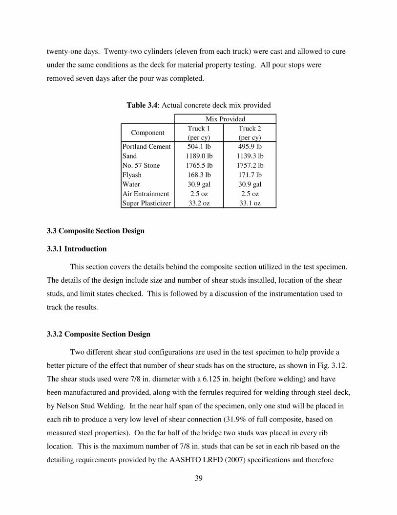
39

twenty-one days. Twenty-two cylinders (eleven from each truck) were cast and allowed to cure

under the same conditions as the deck for material property testing. All pour stops were

removed seven days after the pour was completed.

Table 3.4: Actual concrete deck mix provided

Portland Cement 504.1 lb 495.9 lb

Sand 1189.0 lb 1139.3 lb

No. 57 Stone 1765.5 lb 1757.2 lb

Flyash 168.3 lb 171.7 lb

Water 30.9 gal 30.9 gal

Air Entrainment 2.5 oz 2.5 oz

Super Plasticizer 33.2 oz 33.1 oz

Mix Provided

Truck 2

(per cy)

Truck 1

(per cy)Component

3.3 Composite Section Design

3.3.1 Introduction

This section covers the details behind the composite section utilized in the test specimen.

The details of the design include size and number of shear studs installed, location of the shear

studs, and limit states checked. This is followed by a discussion of the instrumentation used to

track the results.

3.3.2 Composite Section Design

Two different shear stud configurations are used in the test specimen to help provide a

better picture of the effect that number of shear studs has on the structure, as shown in Fig. 3.12.

The shear studs used were 7/8 in. diameter with a 6.125 in. height (before welding) and have

been manufactured and provided, along with the ferrules required for welding through steel deck,

by Nelson Stud Welding. In the near half span of the specimen, only one stud will be placed in

each rib to produce a very low level of shear connection (31.9% of full composite, based on

measured steel properties). On the far half of the bridge two studs was placed in every rib

location. This is the maximum number of 7/8 in. studs that can be set in each rib based on the

detailing requirements provided by the AASHTO LRFD (2007) specifications and therefore

40

produces an upper bound of the level of shear connection (54.2% of full composite based on

measured steel properties) that can be achieved using the Strongweb bridge decking with a

W21x50 steel section. Both levels of shear connection have been checked for compliance with

the AASHTO LRFD (2007) specifications in the fictitious design bridge. The values used for

the static strength of an individual shear stud were calculated based on the equations presented in

the AISC Specification for Structural Steel Buildings (2005), as opposed to the equations given

by AASHTO specifications. This was done because the AISC equations are applicable to studs

welded in ribbed steel decking and therefore account for strong or weak side placement whereas

the AASHTO equations do not. Weak position shear stud strengths were used because there is

less than 2 in. of space between the shank of the stud and the form web at midheight. All

AASHTO LRFD limit states check out except the Fatigue limit state, where the stud spacing for

one stud per rib and two studs per rib, 3.9 in. and 4.75 in. (measured) respectively, is less than

the 8 in. used in the test specimen. This pitch will never be achieved due to the set spacing of the

steel deck forms, which represents another departure from AASHTO LRFD (2007) design.

3.5"

6 .125"

7/8"Shear Stud

Steel Deck

1.0775"

Far Half Span Near Half Span

Figure 3.12: Shear stud layout

3.4 Testing Setup, Instrumentation, and Procedure

3.4.1 Testing Setup

The test setup for all parts of this study is the simply-supported bridge test specimen with

a 30 ft span length. All construction, instrumentation, and testing was completed at the Virginia

Tech Structures Laboratory. Figure 3.13 shows how the specimen girders bear on neoprene

41

bearing pads that have been centered on the girder bearing stiffeners to achieve the simply

supported, 30 ft span required. The bearing pads then rest on W14x99 support beams on the

span ends that are bolted to the reaction floor in the laboratory to prevent movement. This

support setup was chosen because it accurately recreates bearing and support conditions used in

the field and also because the lab already owned reinforced neoprene bearing pads that could be

used for this purpose.

NeopreneBearing Pad

TransverseBrace Angle

W14x99Support Beam

Figure 3.13: Girder bearing details

Two types of bracing were installed to prevent movement of the test specimen during the

cyclic loading of the fatigue tests. To restrain transverse movement, a series of 2.5 in. wide steel

angles (L6x4x3/8) were bolted to the support beam outside of the bearing pads on either side of

the specimen girder bottom flanges, as shown in Fig. 3.13 and 3.14. Two of these angles were

attached at each bearing location and were placed so that the vertical leg bore directly against the

bottom flange, completely restraining all movement. Longitudinal movement was prevented by

bolting a 6 in. long wide flange member to the support beam at the center of the end diaphragm,

as shown in Fig. 3.14. To allow for rotation of the end diaphragm during loading, the

longitudinal bracing was installed so that there was a 0.25 in. clear space between itself and the

specimen end diaphragms.

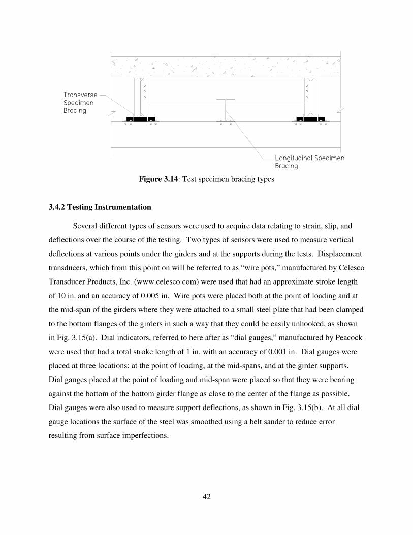
42

TransverseSpecimenBracing

Longitudinal SpecimenBracing

Figure 3.14: Test specimen bracing types

3.4.2 Testing Instrumentation

Several different types of sensors were used to acquire data relating to strain, slip, and

deflections over the course of the testing. Two types of sensors were used to measure vertical

deflections at various points under the girders and at the supports during the tests. Displacement

transducers, which from this point on will be referred to as “wire pots,” manufactured by Celesco

Transducer Products, Inc. (www.celesco.com) were used that had an approximate stroke length

of 10 in. and an accuracy of 0.005 in. Wire pots were placed both at the point of loading and at

the mid-span of the girders where they were attached to a small steel plate that had been clamped

to the bottom flanges of the girders in such a way that they could be easily unhooked, as shown

in Fig. 3.15(a). Dial indicators, referred to here after as “dial gauges,” manufactured by Peacock

were used that had a total stroke length of 1 in. with an accuracy of 0.001 in. Dial gauges were

placed at three locations: at the point of loading, at the mid-spans, and at the girder supports.

Dial gauges placed at the point of loading and mid-span were placed so that they were bearing

against the bottom of the bottom girder flange as close to the center of the flange as possible.

Dial gauges were also used to measure support deflections, as shown in Fig. 3.15(b). At all dial

gauge locations the surface of the steel was smoothed using a belt sander to reduce error

resulting from surface imperfections.

43

Figure 3.15: Vertical deflection sensors (a) support dial gauge placement

(b) in-span dial gauge and wire pot placement

Another method used to monitor loss of stiffness in the specimen was by tracking the

movement of the elastic neutral axis in each fatigue test conducted. This was accomplished

using strain gauges to determine the strain distribution of the section at a given number of cycles.

Strain gauges were placed on the girder prior to the setting of the girders and placement of the

deck so that strain gauge installation was easier. Seven strain gauges were installed at the

quarter spans on both girders, as shown in Fig.3.16. This lead to four total gauge locations

between the two girders, resulting in a total of 28 strain gauges on the test specimen. Gauges

were placed on both girders at the same locations and orientations. Quarter span locations were

chosen because these are the points of loading for the fatigue tests and therefore are the points of

maximum moment. Strain gauges were placed in a vertical line at the locations of interest with

one on the bottom of the bottom flange, one on the bottom of the top flange, three on the exterior

face of the girder, and two on the interior face as shown in Fig. 3.17. The top gauge was placed

on the bottom of the top flange as opposed to the top of the top flange to avoid damaging the

gauge as result of steel deck placement and shear stud welding. Strain gauges used were CEA-

13-250UN-350 gauges produced by Measurements Group, Inc.

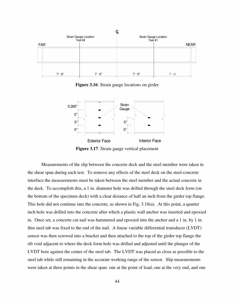
44

Strain Gauge LocationTest #2

Strain Gauge LocationTest #1

CL

7' - 6" 7' - 6" 7' - 6" 7' - 6"

NEARFAR

Figure 3.16: Strain gauge locations on girder

5"

5.265"

Exterior Face Interior Face

5"

5" 5"

5"

StrainGauge

Figure 3.17: Strain gauge vertical placement

Measurements of the slip between the concrete deck and the steel member were taken in

the shear span during each test. To remove any effects of the steel deck on the steel-concrete

interface the measurements must be taken between the steel member and the actual concrete in

the deck. To accomplish this, a 1 in. diameter hole was drilled through the steel deck form (on

the bottom of the specimen deck) with a clear distance of half an inch from the girder top flange.

This hole did not continue into the concrete, as shown in Fig. 3.18(a). At this point, a quarter

inch hole was drilled into the concrete after which a plastic wall anchor was inserted and epoxied

in. Once set, a concrete cut nail was hammered and epoxied into the anchor and a 1 in. by 1 in.

thin steel tab was fixed to the end of the nail. A linear variable differential transducer (LVDT)

sensor was then screwed into a bracket and then attached to the top of the girder top flange the

rib void adjacent to where the deck form hole was drilled and adjusted until the plunger of the

LVDT bore against the center of the steel tab. The LVDT was placed as close as possible to the

steel tab while still remaining in the accurate working range of the sensor. Slip measurements

were taken at three points in the shear span: one at the point of load, one at the very end, and one

45

in the middle of these two, referred to as the mid-shear span. The end slip LVDTs are set up

slightly differently than the two interior sensors as they bear directly against a 1 in. by 1 in. steel

tab epoxied to the deck end, as shown in Fig. 3.18(b). The LVDT’s used were manufactured by

Trans-Tek and had an accuracy of 0.0005 in.

Figure 3.18: LVDT slip sensor setup (a) Interior slip sensor (b) end slip sensor

Additionally, data was collected from the hydraulic actuator LVDT and load cell, which

provided measurements of actuator deflection and load, respectively, to be used in analysis.

Four strain gauges were applied to the top of the concrete deck after fatigue testing had been

completed to track deck strain during the ultimate capacity tests. All data from the strain

gauges, wire pots, LVDT’s, and the actuator load cell during the fatigue testing was collected

through the System 6000 data acquisition system in conjunction with the computer program

StrainSmart 6000, a product of Vishay Measurements. All sensors used in the static testing were

calibrated and collected using a System 5000 scanner (produced by Vishay Measurements) in

conjunction with the Strain Smart 5000 program installed on a lab computer. Once collected,

raw data for the fatigue and static tests were reduced into a Microsoft Excel spreadsheet for

analysis.

3.4.3 Steel Deck Lateral Restraint Testing Procedure

The ability of the steel deck form to act as full compression flange lateral bracing was

investigated during the placement of the specimen concrete deck. To track this, dial gauges were

used to measure both the vertical and lateral deflections once the entirety of the deck had been

poured. Vertical deflections were measured at both quarter-spans and at the mid-span on both

beams, with the reading being measured from the bottom of the bottom flange. Lateral

46

deflection measurements were taken at the midspan of both beams using a steel angle clamped to

the bottom flange, as shown in Fig.3.19. Readings were taken from all dial gauges before deck

placement, immediately after deck placement, and at various times for 14 days following deck

placement to track any movement that occurred during the cure period.

Vertical DeflectionDial Gauge

Horizontal DeflectionDial Gauge

Figure 3.19: Instrumentation for lateral stability test at mid-span

3.4.4 Fatigue Testing Procedure

Two fatigue tests were conducted as part of this research. Each test consisted of a cyclic

loading (following a sine wave function) repeated a set number of times with a different target

load range (the maximum load minus the minimum load) for each test. Each load range is based

on the properties of the specimen quarter-span being tested, as will be discussed later. To track

the degradation of the composite section over the course of each test, static tests were conducted

following the completion of a predetermined number of cycles during which strain, deflection,

and slip data was gathered. The static test intervals roughly followed a log scale with tests

completed after 1, 10, 100, 1000, 10000, 50000, and 100000 cycles. Additional static tests were

conducted after every 100000 cycles until 1.2 million cycles was reached. At each stopping

point, three static tests were conducted. For each static test, an initial compressive load of 1 kip

was applied after which the load was increased at a linear rate until the load on the specimen was

equal to 1 kip greater than the range of the cyclic load being applied for the given fatigue test.

This resulted in a total load increase equal to the value of the cyclic load range. The load was

sustained at this maximum value until the necessary data had been gathered, after which the load

was reduced back to 1 kip at the same linear rate as the increasing load. During each static test,

data from the strain gauges, LVDTs, and wire pots were taken continuously during the entire test

from just before the ramp loading began to just after it ended at the starting load at a rate of 10

47

scans per second using the data acquisition system. Dial gauge deflection readings were taken

by hand at the point of initial load and again at the maximum load as a check for wire pot

deflection values. At every stopping point after 100,000 cycles had been reached, the test

specimen, testing equipment, and load frame were thoroughly inspected for damage resulting

from the fatigue loading to determine if it was safe to continue testing.

For both tests, a 225 kip hydraulic actuator with a 20 in. stroke length connected to a 30

gpm hydraulic power supply was used to apply the cyclic loading during the fatigue tests. The

actuator was mounted in the center of a steel load frame consisting of two vertical columns and

two cross members that were bolted down to the reaction floor to ensure that a closed loading

system was created, seen in Fig. 3.20. To prevent any lateral or longitudinal movement of the

actuator during testing, steel angle bracing was installed that connected the body of the actuator

to the columns of the load frame, also shown in Fig. 3.20. The bracing had a clear distance of

0.75 in. from the actuator body on all four sides with bolts placed through nuts welded to the

angles that bore against the actuator body which made it possible to adjust the actuator location.

Once the actuator was plumb, the bolts were tightened which locked the actuator in place. To

properly distribute the load applied by the actuator to the two specimen girders, the actuator head

was bolted to the center of a 9 ft long, wide flange spreader beam that bore on two 14 in. by 9 in.

by 2.5 in. thick neoprene bearing pads placed on the specimen deck. The neoprene bearing pads

were placed at a 7 ft transverse spacing (3.5 ft from the longitudinal centerline of the bridge) on

the test specimen at the loading point. This was done to ensure that exactly half the load was

transferred directly to each girder while also providing a 2.5 in. clear distance between the deck

and the spreader beam that accounted for deflections in the spreader beam under loading.

48

Spreader BeamFirst Test - W12x 96Second Test - W21x132

Laboratory Reaction Floor

Support BeamW14x99

MTS Actuator

Actuator Bracing

Neoprene Bearing Pad14 in. x 9 in. x 2.5 in.


Figure 3.20: Fatigue testing setup

The first fatigue test took place at the quarter point in the near side mid-span of the test

specimen where shear studs were positioned in a one connector per rib layout. The cyclic loading

for this test was applied at the near side quarter-span location, as shown in Fig. 3.21, so that the

shear studs between the load point and near end of the specimen were receiving the largest

49

horizontal shear and therefore were the most susceptible to fatigue damage. A 50 kip cyclic load

range was calculated for this test based on the AASHTO LRFD (2007) design specification

equation for the spacing of shear connectors under fatigue loading utilizing a 1,000,000 cycle test

length, a shear stud pitch of 8 in. (the rib spacing), a one stud per group layout, and section

properties which had been determined from static tests of the specimen. Details of the

calculations used to determine the load range are given in Appendix B. The test specimen was

loaded cyclically between 5 kips and 55 kips to achieve this range. The cycle rate for the fatigue

loading of 1 Hz was based on the limitations of the hydraulic power supply unit. For the static

tests, the load was ramped from 1 kip to 51 kips in compression at a constant rate of 250 pounds

per second to get the required data. Originally, the first fatigue test was designed to run for

1,000,000 cycles. However, it was later decided to increase the number of cycles to 1,200,000

for two reasons: to determine if trends in the static testing data would continue at the same rate as

was being observed and also to observe specimen behavior beyond the design number of cycles.

Mid-SpanLoadingPosition

End ofSpan

1' - 0"3' - 1"4' - 5"

LVDT(Typ.)

Dial Gauge(Typ.)

Wire Pot(Typ.)

NearSideStrain

Gauges

7' - 6"

Figure 3.21: Fatigue Test 1 details

Figure 3.21 shows the type and locations of the sensors used to acquire the data during

the static tests at stopping points. The sensor layout was exactly the same for both specimen

girders with the one exception that the LVDT slip sensor at the point of loading on girder one

had to be replaced with a dial gauge because the input for that sensor on the data acquisition

system was not functioning properly and would not be fixed in time to be of use in the first test.

Therefore, data for that location was recorded by hand at the same time as the other dial gauges

50

(see above). All dial gauges and wire pots measuring vertical deflection were supported by the

floor of the lab that all of their reference points were the ground. Once testing began, no sensors

were moved from their starting positions to ensure that no error was introduced with regards to

the data taken. All LVDTs and wire pots were zeroed just before testing began. Once testing

had begun, all wire pots and the load input from the actuator load cell were zeroed before every

individual static test conducted. There was no need to zero the dial gauges for this testing.

While the cyclic loading was being applied, all wire pots were detached from the girder bottom

flanges and all dial gauges were clipped so that they were not bearing against the girder bottom

flange. This was done to prevent any damage to sensors due to repeated loading. It was decided

to leave the LVDT sensors in place during cyclic loading because the distance that they move

through is small enough that it would not cause any damage to the sensors. Values for the

applied load were collected from a load cell that was part of the MTS hydraulic actuator.

The second fatigue test performed on the test specimen took place in the far side mid-

span of the test specimen where shear studs were positioned in a two connector per rib layout.

The cyclic loading for this test was applied at the far side quarter-span location, as shown in Fig.

3.22, so that the shear studs between the load point and far end of the specimen were receiving

the highest vertical shear and therefore were the most susceptible to fatigue damage. A 95 kip

cyclic load range was calculated for this test based on the AASHTO LRFD (2007) design

specification equation for the spacing of shear connectors under fatigue loading utilizing a

1,000,000 cycle test length, a shear stud pitch of 8 in. (the rib spacing), a two studs per group

layout, and section properties which had been determined from static tests of the specimen

conducted before the test began. Details of the calculations performed to determine the load

range are given in Appendix B. The test specimen was loaded cyclically between 3.5 kips and

98.5 kips to achieve this range. Due to the large loads being applied to the specimen and the

resulting large deflections, the cycle rate for the second fatigue test had to be reduced to 0.7 Hz.

For the static tests, the load was ramped up from 1 kip to 96 kips in compression at a constant

rate of 500 pounds per second and then back down to 1 kip at the same rate to get the required

data. As was the case with the first test, it was decided to increase the number of cycles by

200,000 above the originally planned 1,000,000 cycles. The goal, again, was to observe whether

trends observed in the design number of cycles would continue past that point and if so, would

they continue at the same rate.

51

Figure 3.22 shows the type and locations of the sensors used to acquire the data during

static tests performed at stopping points. The sensor layout was exactly the same for both

specimen girders. To more accurately account for the compression of the bearing pads at the

girder supports, one additional dial gauge per girder (two total) was added at the near side

support to measure the deflection of the girder bottom flange at the supports farthest from the

point of loading. All other sensors were located as shown and placed in the same way as in the

first fatigue test, described above. All wire pots and dial gauges were again unhooked from the

girder bottom flange during cycling, as in the first test, to prevent causing unnecessary damage to

the sensors.

7' - 6"

End ofSpan

LoadingPosition Mid-Span

End ofSpan

StrainGauges

Dial Gauge(Typ.)

LVDT(Typ.)

NearSide

FarSide

Wire Pot(Typ.)

1' - 0"3' - 2.5" 4' - 3.5"

Figure 3.22: Fatigue Test 2 details

3.4.5 Static Testing Setup and Procedure

Upon completion of the second fatigue test, static tests were conducted at the quarter

points of each half of the test specimen to determine the residual capacity (or plastic moment

capacity) of each type of stud layout to observe how these compare to calculated values. The

static test support conditions were kept the same as in the fatigue testing, with the bridge resting

on 9 in. by 14 in. neoprene bearing pads to create a simply supported condition. Longitudinal

and transverse bracing was also kept in place to ensure that no movement of the test specimen

occurred. The overall test setup is shown in Fig. 3.23.

52

Laboratory Reaction Floor

Support BeamW14x99


Enerpac HydraulicJack


Load Cell

W27x84Cross Members

W21x62 Columns

Steel Distribution Plates

Figure 3.23: Static testing setup

The amount of load required to achieve the ultimate capacity of the specimen was greater

than what could be applied by the 220 kip MTS hydraulic actuator used in the fatigue testing;

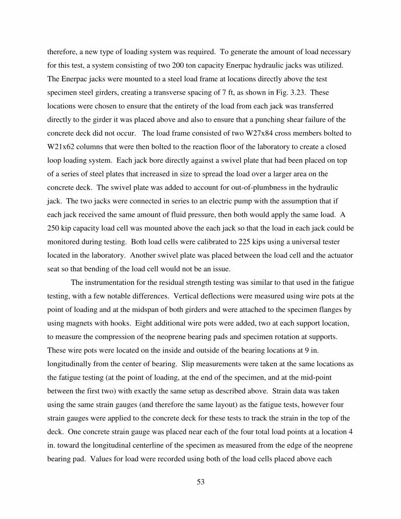
53

therefore, a new type of loading system was required. To generate the amount of load necessary

for this test, a system consisting of two 200 ton capacity Enerpac hydraulic jacks was utilized.

The Enerpac jacks were mounted to a steel load frame at locations directly above the test

specimen steel girders, creating a transverse spacing of 7 ft, as shown in Fig. 3.23. These

locations were chosen to ensure that the entirety of the load from each jack was transferred

directly to the girder it was placed above and also to ensure that a punching shear failure of the

concrete deck did not occur. The load frame consisted of two W27x84 cross members bolted to

W21x62 columns that were then bolted to the reaction floor of the laboratory to create a closed

loop loading system. Each jack bore directly against a swivel plate that had been placed on top

of a series of steel plates that increased in size to spread the load over a larger area on the

concrete deck. The swivel plate was added to account for out-of-plumbness in the hydraulic

jack. The two jacks were connected in series to an electric pump with the assumption that if

each jack received the same amount of fluid pressure, then both would apply the same load. A

250 kip capacity load cell was mounted above the each jack so that the load in each jack could be

monitored during testing. Both load cells were calibrated to 225 kips using a universal tester

located in the laboratory. Another swivel plate was placed between the load cell and the actuator

seat so that bending of the load cell would not be an issue.

The instrumentation for the residual strength testing was similar to that used in the fatigue

testing, with a few notable differences. Vertical deflections were measured using wire pots at the

point of loading and at the midspan of both girders and were attached to the specimen flanges by

using magnets with hooks. Eight additional wire pots were added, two at each support location,

to measure the compression of the neoprene bearing pads and specimen rotation at supports.

These wire pots were located on the inside and outside of the bearing locations at 9 in.

longitudinally from the center of bearing. Slip measurements were taken at the same locations as

the fatigue testing (at the point of loading, at the end of the specimen, and at the mid-point

between the first two) with exactly the same setup as described above. Strain data was taken

using the same strain gauges (and therefore the same layout) as the fatigue tests, however four

strain gauges were applied to the concrete deck for these tests to track the strain in the top of the

deck. One concrete strain gauge was placed near each of the four total load points at a location 4

in. toward the longitudinal centerline of the specimen as measured from the edge of the neoprene

bearing pad. Values for load were recorded using both of the load cells placed above each

54

Enerpac hydraulic jack to permit real time monitoring of applied load in each girder. To allow

for visual confirmation of yielding in the steel girders, the exteriors and bottoms of both girders

were whitewashed using a mixture of lime and water (in a 3:2 ratio, respectively) to a distance of

3 ft on both sides of the point of loading.

The first static test was conducted at the quarter point of the test specimen located in the

near half, where there was a one stud-per-rib layout. Loading and instrumentation details of the

first static test are given in Fig. 3.24. The purpose of this test was to determine the elastic

response of the test specimen with the one stud-per-rib layout. An initial load of 20.0 kips,

approximately 12% of each girder’s near-half calculated plastic capacity of 170.6 kips for each

composite girder, was applied to each girder and then removed to seat the specimen before the

static test began. Details of the calculation of plastic moment capacity are given in Appendix G.

All instruments were zeroed following the seating of the specimen. For the actual test, load was

applied in 5 kip increments until up 65 kips was reached on each girder. At this point, the test

was stopped while the specimen was still in the elastic response region and the specimen

unloaded to prevent causing any significant damage that could negatively affect the results of the

second test. The results of the second test were deemed to be of greater value due to the more

reasonable level of composite action utilized in the two stud-per-rib geometry. The specimen

was unloaded and the load frame moved to the far side quarter point to run the second static test.

Mid-Span

LoadingPosition

End ofSpan

1' - 0"3' - 1"4' - 5"

LVDT(Typ.)

Wire Pot(Typ.)

NearSideStrain

Gauges

7' - 6"

End ofSpan

FarSide

Figure 3.24: Near side static testing details

55

The second static test was conducted at the quarter point of the test specimen located in

the far half, where there was a two stud-per-rib layout. Loading and instrumentation details of

the first static test are given in Fig. 3.25. A load of 26 kips, approximately 15% of the calculated

plastic capacity of 204.2 kips for the far half test specimen, was initially applied and removed to

seat the specimen for the test and then all instruments were zeroed. Details of the calculation of

plastic moment capacity are given in Appendix G. Load was then applied in 5 kip increments

while a plot of the load versus vertical deflection at the point of loading was created. At the

point when the graph began to indicate a non-linear behavioral response of the specimen, the

method of loading was changed from increments of load to increments of deflection. Loading

was continued until a total vertical deflection of 2.75 in. at the point of loading was reached,

where it was determined that the plastic moment had been attained. The specimen was then

unloaded and the load frame and all sensors were moved back into position to load the near half

quarter point.

7' - 6"

End ofSpan

LoadingPosition Mid-Span

End ofSpan

StrainGauges

LVDT(Typ.)

NearSide

FarSide

Wire Pot(Typ.)

1' - 0"3' - 2.5" 4' - 3.5"

Figure 3.25: Far side static testing details

The third static test was conducted back at the quarter point of the specimen located in

the near half, the same location as the first half, with the goal of determining the plastic capacity

of the one stud-per-rib layout. See Fig. 3.24 for details of the loading and sensor layout. The

test was conducted in exactly the same manner as the second static test, with a load controlled

application until a non-linear response was attained followed by a deflection-controlled

application until a deflection of 4 in. had been reached at the points of loading for the girders, at

56

which point it was determined that the plastic moment capacity had been reached. This

concluded all laboratory testing.

57

Chapter 4: Supplemental Testing Results

4.1 Material Properties

4.1.1 Deck Concrete Properties

The composite deck for the test specimen was cast on November 19, 2008 during which 4

in. by 8 in. cylinders were poured from each of the two trucks providing the concrete. The

casting was followed by a 7 day moist cure period after which the pour stops were removed from

the specimen, which was followed by another 21 days of open curing. Every seven days during

the 28 day cure period, cylinders from both batches of concrete (Truck 1 and Truck 2) were

broken to determine the respective compressive strengths, with two cylinders typically being

broken for each test and the results averaged. All testing was conducted at the Virginia Tech

Structures Laboratory. At 28 days, tests were also conducted to determine the modulus of the

elasticity as well as the compressive strength. Comprehensive results of these tests are given in

detail in Appendix C. Table 4.1 gives the measured average compressive strengths, modulus of

elasticity, and the AASHTO LRFD (2007) calculated value (Ec = 33000wc1.5

f’c0.5

) for the

modulus for the given concrete ages. Both trucks batches had a larger average compressive

strength than the target of 4,000 psi specified, with both reaching the target strength by 14 days.

Table 4.1: Deck concrete properties

Truck 1 Truck 2 Truck 1 Truck 2 Truck 1 Truck 2

7 2.26 3.62 - - - -

14 5.01 4.97 - - - -

21 5.31 5.23 - - - -

28 5.89 5.19 4400 4100 4390 4130

Unit Weight = 0.144 kip/ft3

Concrete Age

(days)33,000wc

1.5f’c

0.5

Ec (ksi)f'c (ksi)

Measured

4.1.2 Steel Girder Properties

Material properties for the steel girders used in the test specimen were calculated based

on tensile tests conducted on steel coupons cut from the 3 ft drops of the girders used in the

specimen. Three coupons were cut from each of the flange and the web (six coupons total) of

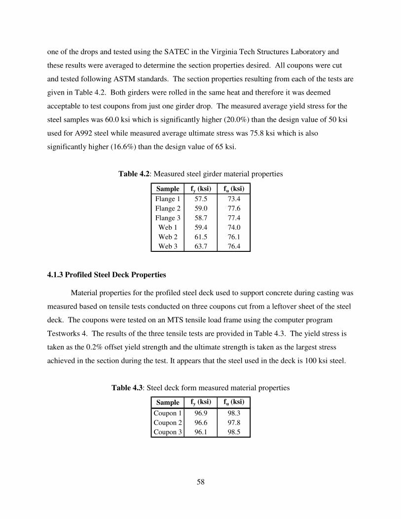
58

one of the drops and tested using the SATEC in the Virginia Tech Structures Laboratory and

these results were averaged to determine the section properties desired. All coupons were cut

and tested following ASTM standards. The section properties resulting from each of the tests are

given in Table 4.2. Both girders were rolled in the same heat and therefore it was deemed

acceptable to test coupons from just one girder drop. The measured average yield stress for the

steel samples was 60.0 ksi which is significantly higher (20.0%) than the design value of 50 ksi

used for A992 steel while measured average ultimate stress was 75.8 ksi which is also

significantly higher (16.6%) than the design value of 65 ksi.

Table 4.2: Measured steel girder material properties

Sample fy (ksi) fu (ksi)

Flange 1 57.5 73.4

Flange 2 59.0 77.6

Flange 3 58.7 77.4

Web 1 59.4 74.0

Web 2 61.5 76.1

Web 3 63.7 76.4

4.1.3 Profiled Steel Deck Properties

Material properties for the profiled steel deck used to support concrete during casting was

measured based on tensile tests conducted on three coupons cut from a leftover sheet of the steel

deck. The coupons were tested on an MTS tensile load frame using the computer program

Testworks 4. The results of the three tensile tests are provided in Table 4.3. The yield stress is

taken as the 0.2% offset yield strength and the ultimate strength is taken as the largest stress

achieved in the section during the test. It appears that the steel used in the deck is 100 ksi steel.

Table 4.3: Steel deck form measured material properties

Sample fy (ksi) fu (ksi)

Coupon 1 96.9 98.3

Coupon 2 96.6 97.8

Coupon 3 96.1 98.5

59

4.2 Lateral Bracing by Steel Deck

This section gives the results from the investigation into whether the steel deck formwork

can be used as a shear diaphragm that acts as continuous lateral compression flange bracing for

the steel girders during the placement of the concrete deck during bridge construction. No

intermediate cross frames or diaphragms were installed on the test specimen to ensure that all

lateral-torsional buckling resistance was provided through a combination of the steel girders and

the stay-in-place form. Based on a method of calculation provided by Helwig and Yura (2008a

and 2008b), a shear diaphragm must provide both adequate stiffness and strength. With regards

to diaphragm stiffness, it was determined that an effective shear modulus of 6.25 kip/in was

required to prevent lateral-torsional buckling in the test specimen during construction. For the

chosen steel deck form, 20 gage Strongweb supplied by Wheeling Corrugating, the provided

effective shear modulus was 34.6 kip/in., easily satisfying the stiffness requirement. In terms of

strength, based on the five edge fastener pattern over the form cover width of 32 in., a critical

connector strength of 0.932 kips is required at the edge fasteners. Each shear connector has a

welded strength of 39.1 kips, so therefore breaking the shear connector weld is not an issue. The

failure mode of the steel deck form is expected to be bearing and tear-out. The strength of the

form in the one stud-per-rib half span is 7.39 kips, which is taken as the critical value for this

investigation. Therefore, the strength requirements are met. All supporting calculations for this

section are provided in Appendix D.

With regards to the test specimen behavior, no issues were encountered during the

placement of the concrete deck. Both girders produced similar results, indicating similar

behavior from both samples. Dial gauges placed to measure the lateral movement of the bottom

flange of the steel girders during the concrete deck placement indicated that the Girder 1 bottom

flange deflected 0.263 in. outward from the longitudinal centerline of the specimen at mid-span

and Girder 2 deflected 0.262 in. outward at mid-span. Both the Girder 1 and Girder 2 deflections

represent 0.31% of the span of the form, which is the girder spacing (84 in.). It is important to

point out that these results could be skewed slightly due to the fact that the timber kickers used to

support the deck overhangs during casting (see section 3.2.3) bore against the bottom flange of

the steel girders and could possibly have applied a resisting force to the outward movement of

the bottom flange. This could have reduced the lateral deflections of the bottom flange.

However, it is unlikely that this would have had a significant effect on the results due to the fact

60

that the timber kickers were loose at the time of their removal, indicating that very little load was

applied to the steel girder bottom flange.

4.3 Non-Prismatic Beam Deflection Analysis

As a means of comparing calculated elastic deflections to values measured during testing,

early models were created that assumed constant section properties throughout the entirety of the

test specimen (prismatic) based on the properties of the specimen half being testing. This means

that for tests conducted on the half of the test specimen with one stud per rib (near half), the

moment of inertia for the entirety of the specimen was taken as the value produced by the AISC

commentary (2005) effective moment of inertia equation using the appropriate level of shear

connection (Inear = 3344.1 in4). Likewise, for tests conducted on the half of the specimen with

two studs per rib (far half), the moment of inertia for the entirety of the test specimen were taken

as the effective moment of inertia using the given level of shear connection here (Ifar = 4062.4

in4). However, the assumption of a prismatic section will not produce accurate deflection results.

For testing on the near side, the actual specimen deflections will be lower than predicted because

the far half has a higher moment of inertia than the near half and therefore the stiffness will be

slightly greater than in the prismatic model. Conversely, because the near half moment of inertia

is less than that of the far half, the actual specimen stiffness will be slightly less than predicted in

the prismatic model and will produce higher deflections.

As a means of taking into account the two different section properties of the test

specimen, a new model using a non-prismatic section was created to calculate the deflections of

the test specimen under the calculated moment capacity loads in the near half and far half. This

model utilized both calculated values for the moment of inertia in their respective halves to

calculate deflections, as shown in Fig. 4.1. The analysis of the section was performed using the

Elastic Load Method. The predicted values were calculated for both the fatigue test loadings and

the static test loading. The results of the analysis for the fatigue tests are provided in Table 4.4

while results of the analysis for the static tests are provided in Table 4.5. ASIC (2005)

recommends a reduction a 25% be applied to the calculated effective moments of inertia so

deflection results were taken for both 75% of respective halves’ calculated moments of inertia as

well as 100% of the calculated moments of inertia. This was done to evaluate which level of

stiffness more accurately predicts the deflections measured in testing. Values shown are for the

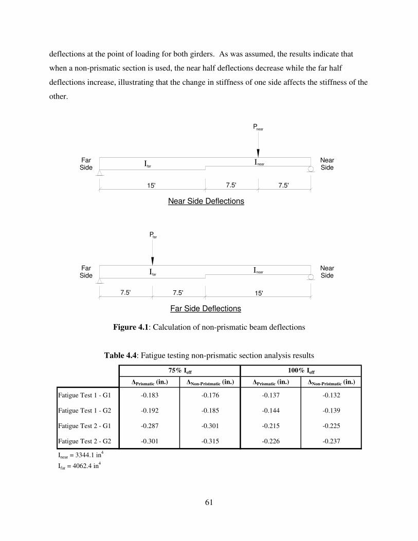
61

deflections at the point of loading for both girders. As was assumed, the results indicate that

when a non-prismatic section is used, the near half deflections decrease while the far half

deflections increase, illustrating that the change in stiffness of one side affects the stiffness of the

other.

7.5'7.5'15'

InearIfar

Pnear

NearSide

FarSide

7.5'7.5' 15'

InearIfar

Pfar

NearSide

FarSide

Near Side Deflections

Far Side Deflections

Figure 4.1: Calculation of non-prismatic beam deflections

Table 4.4: Fatigue testing non-prismatic section analysis results

∆Prismatic (in.) ∆Non-Pristmatic (in.) ∆Prismatic (in.) ∆Non-Pristmatic (in.)

Fatigue Test 1 - G1 -0.183 -0.176 -0.137 -0.132

Fatigue Test 1 - G2 -0.192 -0.185 -0.144 -0.139

Fatigue Test 2 - G1 -0.287 -0.301 -0.215 -0.225

Fatigue Test 2 - G2 -0.301 -0.315 -0.226 -0.237

Inear = 3344.1 in4

Ifar = 4062.4 in4

75% Ieff 100% Ieff

62

Table 4.5: Static testing non-prismatic section analysis results

∆Prismatic (in.) ∆Non-Pristmatic (in.) ∆Prismatic (in.) ∆Non-Pristmatic (in.)

Static Tests 1 and 3 -1.28 -1.23 -0.961 -0.924

Static Test 2 -1.26 -1.32 -0.948 -0.993

Inear = 3286.5 in4

Ifar = 3985.9 in4

75% Ieff 100% Ieff

63

Chapter 5: Laboratory Fatigue Testing Results

5.1 Fatigue Test 1

5.1.1 Overview

This section provides an overview of the results from the first fatigue test performed on

the test specimen. As previously stated, this test was performed at the near side quarter span

location and consisted of a 50 kip range loading (from 5 to 55 kips) repeated for 1.2 million

cycles at a rate of 1.0 Hz with three ramped loading tests from 1 kip to 51 kips at a rate of 250

lb/sec (loading and unloading) conducted at every predetermined cycle interval.

No major problems were encountered with the test specimen during the course of this

test. Various inspections conducted during the testing period revealed no signs of cracking in

either the steel girders or concrete deck, which was expected as the loading was well within the

working range of the structure. However, major problems occurred with the testing equipment

that resulted in major delays in the test. At approximately 92,000 cycles, the oil pump in the

hydraulic supply stopped working and had to be replaced. It took approximately 7 weeks to

replace this part and get the pump back in working order. During this period, the actuator was

connected to a smaller hydraulic power supply (HPS) unit (11 gpm) and run at a rate of 0.5 Hz

for an additional 150,000 cycles (to ~240,000 total cycles) at which point it was decided that the

output demand was too large for the smaller HPS and could cause significant damage to the unit

if testing continued and therefore the actuator was disconnected. Testing did not continue until

the original HPS was fixed. The remainder of the first fatigue test was completed without any

further equipment issues.

To track loss of stiffness in the test specimen under repeated loading, dial gauges (DG)

and wire pots (WP) were used to measure vertical deflection, linear variable differential

transducers (LVDT) were used to measure slip at the steel/concrete interface, and strain gauges

(SG) were used to measure strain at various points in the steel girder cross section. The sensors

were distributed as described in Chapter 3 of this thesis and were labeled as shown in Fig. 5.1.

The remainder of this thesis pertaining to the first fatigue test will follow these labeling

conventions.

After the first fatigue test had begun, it was discovered that the test specimen had been

built slightly off center of the load frame. Due to the large weight of the test specimen, this shift

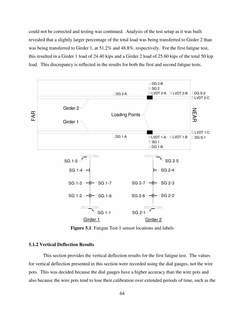
64

could not be corrected and testing was continued. Analysis of the test setup as it was built

revealed that a slightly larger percentage of the total load was being transferred to Girder 2 than

was being transferred to Girder 1, at 51.2% and 48.8%, respectively. For the first fatigue test,

this resulted in a Girder 1 load of 24.40 kips and a Girder 2 load of 25.60 kips of the total 50 kip

load. This discrepancy is reflected in the results for both the first and second fatigue tests.

Girder 2

Girder 1

NE

AR

FA

R

DG 2-A

DG 2-B

SG 2

LVDT 2-A

LVDT 1-B

LVDT 1-CDG 1-A

DG 1-B

LVDT 1-A

LVDT 2-B

LVDT 2-C

SG 1

Loading Points

DG S-2

DG S-1

SG 1-1

SG 1-6

SG 1-3

SG 1-2

SG 1-7

SG 1-5

SG 1-4

SG 2-1

SG 2-6

SG 2-3

SG 2-2

SG 2-7

SG 2-5

SG 2-4

Girder 1 Girder 2

Figure 5.1: Fatigue Test 1 sensor locations and labels

5.1.2 Vertical Deflection Results

This section provides the vertical deflection results for the first fatigue test. The values

for vertical deflection presented in this section were recorded using the dial gauges, not the wire

pots. This was decided because the dial gauges have a higher accuracy than the wire pots and

also because the wire pots tend to lose their calibration over extended periods of time, such as the

65

time it takes to complete a fatigue test, whereas this is not the case with dial gauges. Wire pot

data was still collected, but only to act as a backup for dial gauge measurements.

Values for vertical deflection were collected at the mid-span, point of loading, and at the

near side supports for each static test at the point before loading and at the ultimate load. The

dial gauges at the supports were meant to measure the deflection of the neoprene bearing pads

and the support beams under the loading so that these deflections could be accounted for in the

calculations of the actual specimen deflection. It was assumed for this analysis that the far side

neoprene bearing pads behaved the same under loading as the near side bearing pads and

therefore, given the load location for this test, would deflect three times less than the near side

bearing pads (which are three times closer to the point of loading). The difference between the

near and far side bearing pad deflections was then scaled down based on the sensor location

being examined (0.75 for the point of loading and 0.5 for the mid span), added to the lesser

support deflection, and then subtracted from the measured deflections at their respective

locations. Sample vertical deflection calculations are given in Appendix E. Once the absolute

deflections for every sensor in each of the three static tests conducted at each stopping point had

been calculated, the three values of the individual sensors were averaged to produce the results

presented in this section. This was done to ensure repeatability in the testing. Absolute

deflection values for the same sensor in each of the three static tests were almost always very

close if not the same.

The actual vertical deflection results for Fatigue Test 1 are provided in Table F.1in

Appendix F. The percent change given is the increase or decrease in deflection at a given

number of cycles as compared to the initial values measured at 1 cycle. Both girders lost very

little stiffness over the course of the testing and it appears that no significant damage was done to

the test specimen over the course of this fatigue test. At the fatigue design life (one million

cycles), the deflections in Girder 1 at the mid-span (1-A) and at the point of loading (1-B) only

increased by values of 4.08% and 4.58%, respectively. These percentages increased to 4.99%

for location 1-A and 5.30% for 1-B at the 1,200,000 cycle mark, indicating a minor increase in

deflections that were similar to changes in deflection over a 200,000 cycle period at other points

in the test and therefore the author assumed that this was not indicative of any increased damage

following the end of the design life.

66

Girder 2 presented similar results to Girder 1. At the fatigue design life, the percent

increase in Girder 2 at location 2-A (mid-span) was 5.54% while at 2-B (point of loading) it was

5.41%. These values then increased to 6.77% at 2-A and 7.25% at 2-B at 1,200,000 cycles. The

percent increase at both locations was slightly greater than that of their counterparts in Girder 1,

which is possibly due to the fact that Girder 2 is receiving slightly more of the total load, as

explained above, and is therefore being fatigued to a greater degree. Again, though, the results

presented here do not indicate that significant damage has occurred to the system or that any kind

of failure is imminent.

Figure 5.2 provides a plot of the adjusted vertical deflections at each sensor location

(corrected for support effects) under the 50 kip loading versus the number of cycles for both the

mid-span (A) and the point of loading (B) locations. The group of two lines with the lower

values represents the vertical deflection at the point of loading locations, 1-B and 2-B, while the

group with the higher values represents the vertical deflection at the mid-span locations, 1-A and

2-A. As can be seen, from 1 to 50,000 cycles, the deflections in both girders increase at a rate

faster than any other time during the test, which seems to indicate that some settling of the test

specimen occurred during this time period. It is assumed that pockets were formed in the

concrete adjacent to the shear stud shanks during this settling period which lead to large slips in

the composite system causing the loss of stiffness and increased deflections until the concrete

compacted and stabilized around the studs and slips stopped increasing. This assumption is

supported by the slip results (presented in later sections) which show large increases in slip until

100,000 cycles were reached when the slip values at all three locations began to level off or even

decrease. After the 50,000 cycle mark, both girders behaved similarly over the course of testing,

and appear to lose stiffness at about the same rate with the increase in deflection per number of

cycles appearing to be almost linear for all locations on both girders. Figure 5.2 also shows that

at the design number of cycles, there was no significant jump in the rate of the increase in

vertical deflection in Girder 1 while there was only a slight increase in Girder 2, which will be

addressed in the elastic neutral axis results.

67

Number of Cycles (N)

200000 400000 600000 800000 1000000 1200000

∆ (

in.)

-0.16

-0.14

-0.12

-0.10

-0.08

-0.06

-0.04

-0.02

0.00

Mid-Span - Girder 1

Point of Load - Girder 1

Mid-Span - Girder 2


Figure 5.2: Vertical deflection results for 50 kip loading in Fatigue Test 1

It is important to note that the initial deflections for both girders at all locations were

lower than was predicted for the given level of composite action. Figure 5.3 provides a plot of

the measured deflection values at the point of loading normalized to the calculated values of

deflection at this point using both 75% and 100% of the effective moment of inertia as provided

by the AISC commentary provisions (2005) for both girders in Fatigue Test 1. As can be seen,

the measured deflections are less than the calculated deflections for both values of the effective

moment of inertia over the entirety of the test. These results indicate that the predicted moments

of inertia were conservative for the level of composite action present in the system (at 32%

composite) even at the end of testing. The unreduced effective moment of inertia provides a

more accurate prediction of the deflections while still remaining slightly on the conservative

side.

68


0 200000 400000 600000 800000 1000000 1200000

∆/∆

p

0.0

0.1

0.2

0.3

0.4

0.5

0.6

0.7

0.8

0.9

1.0

Normalized Girder 1 - 75% Ieff




Figure 5.3: Point of loading deflections normalized to predicted values in Fatigue Test 1

As a way of predicting what the deflection response will be at points in the specimen life

beyond the number of load cycles applied during testing, curves were fit to the deflection data

for each girder at the point of loading. Two different types of curves were fit to the deflections

for each girder that reflected different types of specimen response and then were extrapolated to

five million cycles, as shown in Fig.5.4. The first curve was one where the deflections

approached an asymptotic value and then leveled off as a means of showing where the system

might stabilize. The second line is one where the trends observed during the test continued in a

linear fashion to show where the deflections would end up if the loss of stiffness stayed constant.

The results of this analysis are given in Table 5.1. The point of total shear stud failure occurs

when there is no composite action between the deck and the girders, which means that the girder

is taking the entire load. The deflection corresponding to this non-composite state at a load of 25

kips is -0.479 in. As can be seen, at five million cycles, the maximum values for deflection in

both girders are still less than half of the non-composite deflection. The Girder 2 deflections

reach a higher value than in Girder one, with the maximum increase in deflection representing

about 25% of the initial value. This shows increased damage in Girder 2, a fact which is

69

reflected in the testing. These results indicate that there is still a significant amount of residual

strength and stiffness at five times the design number of cycles.


0 1000000 2000000 3000000 4000000 5000000

Extr

ap

ola

ted

De

fle

ctio

n (

in.)

-0.20

-0.18

-0.16

-0.14

-0.12

-0.10

-0.08

-0.06

-0.04

-0.02

0.00

Constant Increase - Girder 1

Level Off - Girder 1



Calculated Deflection - 75% Ieff

Calculated Deflection - 100% Ieff

Figure 5.4: Vertical deflections extrapolated to 5 million cycles in Fatigue Test 1

Table 5.1: Vertical deflection extrapolation results for Fatigue Test 1

1 Cycle

∆1 cycle (in.) ∆1,000,000 cycles (in.) % Change ∆5,000,000 cyles (in.) % Change

Girder 1 - Level -0.1148 -0.1200 4.53% -0.1222 6.45%

Girder 1 - Constant -0.1148 -0.1200 4.53% -0.1298 13.07%

Girder 2 - Level -0.1147 -0.1209 5.41% -0.1311 14.30%

Girder 2 - Constant -0.1147 -0.1209 5.41% -0.1428 24.50%

5,000,000 Cycles1,000,000 CyclesLocation

5.1.3 Slip Results

The interface slip values measured during Fatigue Test 1 are provided in Table F.2 in

Appendix F. These results are shown plotted in Figs. 5.5 and 5.6 below for Girders 1 and 2,

respectively. At the beginning of testing, the slips in both girders increased rapidly in the first

50,000 cycles at about the same values at which point they leveled off slightly, indicating settling

in the test specimen as noted in the vertical deflection results. Once the test specimen had

settled, slip values at the end of the span (location C) and at the mid-point of the shear span

70

(location B) for both girders increased at a non-linear rate, with that rate increasing as the test

moved forward, indicating that the slip was getting larger for the same number of cycles as the

test continued. What is interesting is that the slip at both locations increased at nearly the same

rate, with each following almost the exact same trend for both girders, indicating that once the

girder had settled the increase in slip was consistent for the entire shear span outside of the large

interface friction zone near the point of loading. At the point of loading (location A), the

increase in slip was significantly less than at the other locations for Girder 2, as was expected

due to how close it was to the point of maximum moment and the resulting effects of interface

friction. The slip at location A stayed relatively constant until 1 million cycles had been reached,

at which point it increased rapidly along with locations B and C, possibly indicating that the

friction force had been overcome. Slip at location A on Girder 1 was recorded using a dial gauge

and it does not appear that the data taken was as consistent as it should have been, as evidenced

by the sudden jumps in slip values, and therefore is taken as inadmissible.


0 200000 400000 600000 800000 1000000 1200000

Slip

(in

.)

-0.0020

-0.0015

-0.0010

-0.0005

0.0000


Mid-Shear Span - Girder 1

End of Span - Girder 1

Figure 5.5: Interface slip results at 50 kips in Girder 1 in Fatigue Test 1

71


0 200000 400000 600000 800000 1000000 1200000

Slip

(in

.)

-0.0030

-0.0025

-0.0020

-0.0015

-0.0010

-0.0005

0.0000

Point of Loading - Girder 2




Slip values for Girder 1 were lower than those in Girder 2 at the same locations for the

entirety of the test. However, the values of slip are still so small that this does not appear to be

indicative of any large inconsistency between the two girders. The only major change in the slip

trends of the girders (after settling had occurred) came in Girder 2 at locations B and C between

700,000 and 1,000,000 cycles when the rate of slip increases suddenly and then levels off. At

1,000,000 cycles the rate increases suddenly again, however it appears that the trends return to

where they were going before the change occurred at 700,000 cycles. This shift had a larger

effect on the slip at the end of the span, therefore it is believed that a single shear stud or a group

of shear studs near the end of the span in Girder 2 caused some slight crushing of the concrete

around the shank of the stud, resulting in the larger slip values noted. The slip leveled off once

the crushing was complete due to the restraint imposed by the rest of the shear studs in the shear

span. Once slip had increased in the rest of the shear span to a point where the studs were in

contact with the concrete again, the increase in slip resumed the path it had been following

previously. This increase at 1,000,000 cycles also correlates with increases in deflection and

movement of the elastic neutral axis.

72

One very important feature of the results to point out is that for both girders, the slip at

the end of the span is less than the slip at the point mid-way between the point of loading and the

end of the span, which is the opposite of what was expected. Typically, the slip is the smallest at

the loading and then increases as you approach the end of the span, where it is the largest. It is

unknown why this occurred in the system; however, due to the consistency of the trends within

each individual girder and also between the two girders themselves, it was determined that there

was not any error made in collection of the data.

In examining the results presented, it is important to discuss where the slips seem to be

going. Based on Figs. 5.5 and 5.6 above, the rate of increase of the slip (slope of the line) has

been increasing the entirety of the test and shows no sign of leveling off at a point past the

number of load cycles applied, with this effect being more severe in Girder 2 than in Girder 1.

The increase in slip is what leads to the loss of composite action between the steel girder and the

concrete slab resulting in the loss of stiffness. Therefore, it can be concluded that the amount of

slip will most likely continue to rise, along with the vertical deflections, unless stabilization of

the system occurs. There is not a direct correlation between the increase in slip and the increase

in deflection, so if the slips continue to increase, it is likely that the vertical deflections will

continue to increase at the same rate as observed in testing until shear stud failures begin. It is

important to note that this failure point would be well beyond the design fatigue life of the given

specimen. Within the design fatigue life, the slips are still very small and it can be concluded

that no significant damage has occurred to the system.

In examining the slip results, a possible beneficial effect is observed. As the amount of

slip increases, the shear stud shank spends less time in contact with the surrounding concrete

because the pocket being formed by the cycles is getting larger. As result, it is possible that the

shear range on the shear studs decreases over time as the slip increases which could lead to an

increase in the specimen fatigue life. However, at this stage the effect is purely speculation.

Research is required to determine if it does exist and what the resulting behavioral results are.

5.1.4 Strain Results

This section provides the results of the analysis of the seven strain gauges placed

vertically at the point of loading (near side quarter point), as shown in Fig. 5.1. No issues were

encountered with measurements provided by the strain gauges due to the fact that the applied

73

load was well within the linear elastic range of the composite system and therefore all gauges

were used in the analysis. Tables F.3 and F.4 provided in Appendix F gives the calculated values

for every strain gauge location as well the their relative change given as a percentage of the

gauge values at 1 cycle (the beginning of testing) for Girder 1 and Girder 2, respectively.

Results presented for each gauge location at each cycle interval represent an average of the

measured values for each gauge from the three static tests conducted at each stopping point.

These results are shown plotted for Girder 1 in Fig. 5.7 and for Girder 2 in Fig. 5.8 and show that

the change in strain over time is approximately linear. These tables and plots illustrate that the

change in strain at each gauge location is minimal over the course of the test for both girders, as

indicated by the very minor slope of each line. There were no significant jumps in values at any

location on either girder that would result from a change in the composite system, such as the

breaking of a shear stud, and therefore it can be implied that a minimal amount of damage was

done to the system over the course of the first test. Both girders behavior was almost exactly the

same during the test, with the percent changes in Girder 2 being slightly higher than those in

Girder one, which can be accounted for by the larger Girder 2 load. These results correlate

almost exactly with vertical deflection results for both girders.


0 200000 400000 600000 800000 1000000 1200000

Str

ain

(µ

ε)

0

50

100

150

200

250

300

SG 1-1

SG 1-2

SG 1-3

SG 1-4

SG 1-5

SG 1-6

SG 1-7

Figure 5.7: Strain results for 50 kip loading in Girder 1 in Fatigue Test 1

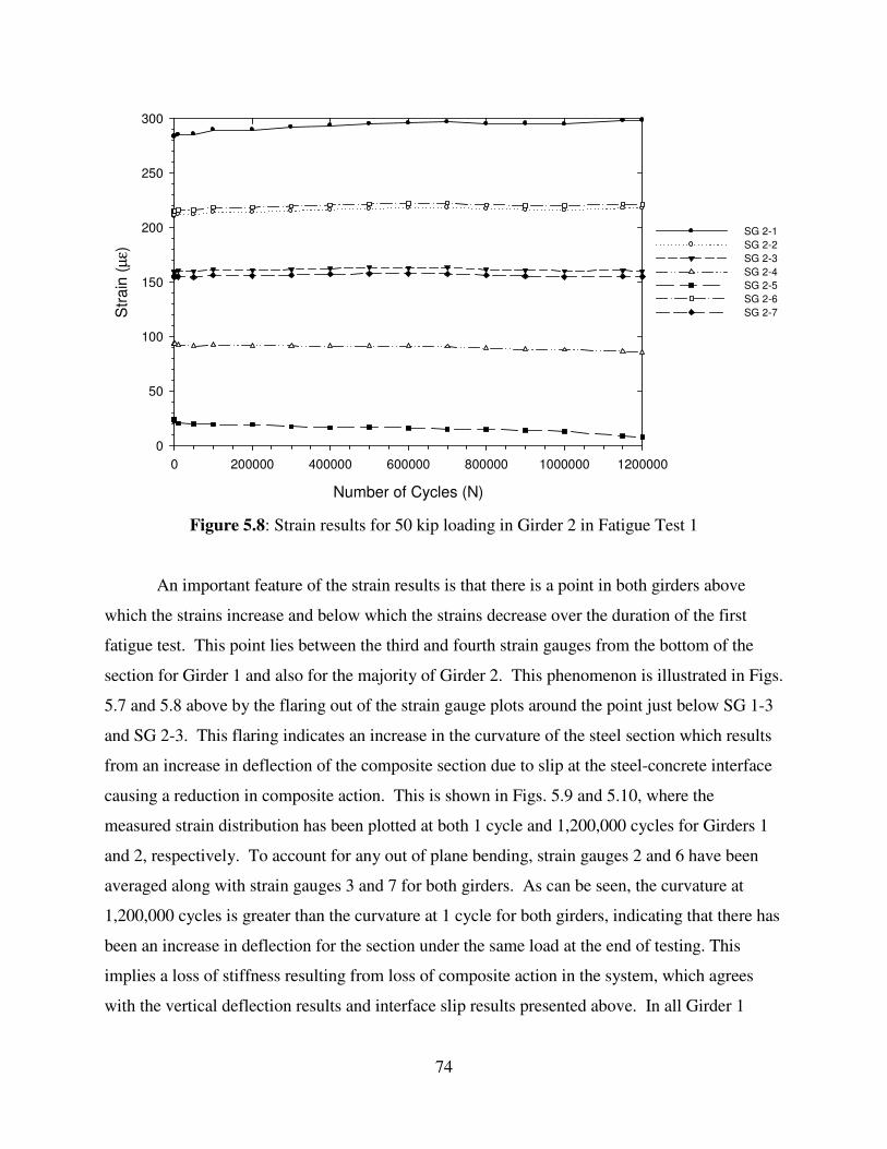
74


0 200000 400000 600000 800000 1000000 1200000

Str

ain

(µ

ε)

0

50

100

150

200

250

300

SG 2-1

SG 2-2

SG 2-3

SG 2-4

SG 2-5

SG 2-6

SG 2-7


An important feature of the strain results is that there is a point in both girders above

which the strains increase and below which the strains decrease over the duration of the first

fatigue test. This point lies between the third and fourth strain gauges from the bottom of the

section for Girder 1 and also for the majority of Girder 2. This phenomenon is illustrated in Figs.

5.7 and 5.8 above by the flaring out of the strain gauge plots around the point just below SG 1-3

and SG 2-3. This flaring indicates an increase in the curvature of the steel section which results

from an increase in deflection of the composite section due to slip at the steel-concrete interface

causing a reduction in composite action. This is shown in Figs. 5.9 and 5.10, where the

measured strain distribution has been plotted at both 1 cycle and 1,200,000 cycles for Girders 1

and 2, respectively. To account for any out of plane bending, strain gauges 2 and 6 have been

averaged along with strain gauges 3 and 7 for both girders. As can be seen, the curvature at

1,200,000 cycles is greater than the curvature at 1 cycle for both girders, indicating that there has

been an increase in deflection for the section under the same load at the end of testing. This

implies a loss of stiffness resulting from loss of composite action in the system, which agrees

with the vertical deflection results and interface slip results presented above. In all Girder 1

75

results and most of the Girder 2 results, there are no significant jumps in strain values and all

strain gauge plots are nearly linear, which further correlates with the vertical deflection results

from the point of loading location. The only visible departure from linearity in strain

degradation comes in Girder 2 between 1,000,000 cycles and 1,150,000 cycles where the rate of

change in all the gauges increases suddenly, which correlates with a slight jump in deflection and

elastic neutral axis location, which is explained below. This is more than likely the result of the

jump and then leveling off of slip observed in Girder 2 as noted in the “Slip Results” section.

Strain (µε)

0 50 100 150 200 250 300

Vert

ical Location (

in.)

0

5

10

15

20

25

Strain at 1 Cycle - Girder 1

Strain at 1,200,000 Cycles - Girder 1

Top of steel section

Figure 5.9: Vertical strain distribution at 50 kips in Girder 1 in Fatigue Test 1

76

Strain (µε)

0 50 100 150 200 250 300

Vert

ical Location (

in.)

0

5

10

15

20

25

Strain 1 Cycle - Girder 2

Strain 1,200,000 Cycles - Girder 2


Figure 5.10: Vertical strain distribution at 50 kips in Girder 2 in Fatigue Test 1

The increase in curvature, and subsequently the increase in deflections, is also reflected

in the movement of the elastic neutral axis of the steel girder toward the bottom of the section,

shown in Fig. 5.11. The elastic neutral axis is the location in the girder cross-section where the

strain is equal to zero while the loading is still in the linear elastic range. To calculate the elastic

neutral axis, a least squares linear regression line was fitted to the strain values at the points

going up the steel girder cross-section at a given number of cycles. Once the equation of this

line was known, the value of the Y-axis intercept point is the elastic neutral axis. The elastic

neutral axis of the fully composite section represents an upper bound for this value and has been

calculated as 25.1 in. from the bottom of the composite section. Likewise, the lower bound of

the steel girder elastic neutral axis comes when there is no interaction between the steel girder

and concrete deck and for that reason it is the centroid of the steel girder, which is 10.4 in. from

the bottom of the section. Therefore, as the level of composite action of the system decreases

due to increased slip at the interface, the elastic neutral axis (ENA) of the steel girder will lower

accordingly as the system loses stiffness.

77

It should be noted that at no point during the testing was the measured ENA at or below

the top of the steel section and therefore there is no true neutral axis for the steel girders, as

illustrated by the horizontal line marking the top of the girder in Fig. 5.11. This means that the

slip at the interface has not become large enough to cause a compressive stress in the top of the

steel girder. However, the term elastic neutral axis will be used to denote where the strain

distribution in the steel crosses the zero point and will be used to track degradation of composite

action in the test specimen.

As can be seen in Fig. 5.11, the calculated elastic neutral axis (ENA) falls within the

upper and lower bounds given, indicating partial composite action as expected. The ENA

dropped rapidly in the first 50,000 cycles for both girders as the test specimen settled; however

after this point in the testing it leveled out and then approached the bottom of the section at a

nearly linear rate, with values and rate of decrease in Girder 2 slightly greater than that in Girder

1, which agrees with slip data presented previously (Girder 2 slip values are greater and increase

faster than Girder 1 values). At the end of the design number of cycles (1,000,000), the ENA in

Girder 1 only dropped 0.77 in., which represents only 3.7% of the steel girder depth, with 45.5%

of the movement occurring in the first 50,000 cycles (5% of the total cycles). The same trend

continued in Girder 1 to 1.2 million cycles. Likewise, through the design number of cycles in

Girder 2, the ENA dropped 0.93 in., representing 4.5% of the total number of cycles with 32.3%

of that movement occurring in the first 50,000 cycles. However, after 1 million cycles the rate of

decrease of the ENA increased in Girder 2, with the change becoming 1.32 in. from initial

position, which is 6.3% of the steel girder depth. This increase correlates with jumps in strain

gauge and deflection values noted previously and is explained by the fact that the rate of slip

increased at all measured locations at that point as well, which caused the slight loss of

composite action that resulted in the loss of stiffness and therefore the increase in deflection and

movement of the ENA. However, this loss of stiffness is still minor. This increase in slip was

not observed in Girder 1 and therefore the ENA did not drop in the same way as in Girder 2.

Based on these results, there is no indication that significant damage has been done to the system

as a result of the fatigue loading on either girder, especially within the design number of cycles.

78


0 200000 400000 600000 800000 1000000 1200000

Locatio

n o

f N

eutr

al A

xis

(in

.)

0

5

10

15

20

25

Neutral Axis Girder 1



Figure 5.11: Steel girder elastic neutral axis from bottom of section in Fatigue Test 1

5.2 Fatigue Test 2

5.2.1 Overview

This section provides an overview of the results from the first fatigue test performed on

the test specimen. This test was performed at the far side quarter span location and consisted of

a 95 kip range loading (from 3 to 98 kips) repeated for 1.2 million cycles at a rate of 0.68 Hz

with three ramped static loading tests from 1 kip to 96 kips at a rate of 500 lb/sec (loading and

unloading) conducted at every predetermined cycle interval.

No problems were encountered with the test specimen during the course of this test.

Various inspections conducted during the testing period revealed no signs of cracking in the steel

girders and only some very small fatigue cracks in the concrete deck localized to the loading

areas, which was expected as the loading was still within the working range of the structure.

There were no issues with the testing equipment in this fatigue test and therefore the entire test

was completed with no delays. As in the first test, the test specimen was slightly off center with

respect to the load frame which lead to Girder 2 receiving more of the total load than Girder 1

79

(51.2% and 48.8%, respectively, based on a static analysis). This resulted in a Girder 1 load of

46.4 kips and a Girder 2 load of 48.6 kips.

The instrumentation utilized for the second fatigue test was almost exactly the same as

was used the first test, with the only difference being that two additional dial gauges were added

to the supports farthest away from the point of loading. This was done so that more accurate

calculations for the absolute vertical deflections at the point of loading and mid-span could be

made. The sensor were placed and labeled as shown in Fig. 5.12. The remainder of this thesis

pertaining to the second fatigue test will follow these labeling conventions.

Girder 2

Girder 1

NE

AR

FA

R

DG 2-A

DG 2-B

SG 4

LVDT 2-A

LVDT 1-B

LVDT 1-CDG 1-ALVDT 1-A

LVDT 2-B

LVDT 2-C

SG 3

DG 1-B

Loading Points

DG S-2

DG S-1

DG S-2b

DG S-1b

SG 3-1

SG 3-6

SG 3-3

SG 3-2

SG 3-7

SG 3-5

SG 3-4

SG 4-1

SG 4-6

SG 4-3

SG 4-2

SG 4-7

SG 4-5

SG 4-4

Figure 5.12: Fatigue Test 2 sensor locations and labels

80

5.2.2 Vertical Deflection Results

This section provides the vertical deflection results for the second fatigue test. As with

Fatigue Test 1, the results presented in this section were calculated from the dial gauge readings,

not wire pot data. Values for vertical deflection were taken at the mid-span, point of loading,

and at both supports. Calculation of absolute deflections in this test were simpler than those in

Fatigue Test 1 as there was no need to make assumptions about the deflections of the supports

farthest away from the point of loading. To calculate the absolute deflections, the difference

between the far and near side bearing pad deflections was scaled down based on the sensor

location being examined (0.75 for the point of loading and 0.5 for the mid span), added to the

near side support deflection, and then subtracted from the measured deflections at their

respective locations. See Appendix E for sample calculations. As in Fatigue Test 1, three static

tests were conducted at each stopping point and the calculated values for absolute deflections at

the mid-span and point of loading was averaged to produce the results presented here.

The vertical deflection results for Fatigue Test 2 are provided in Table F.6 in Appendix F.

The percent change given is the increase or decrease in deflection at a given number of cycles as

a percentage of the values measured at 1 cycle. As can be seen, a small amount of stiffness was

lost over the course the course of the fatigue testing, with Girder 1 results very similar to those

from the first test and Girder 2 having a slightly larger percentage increase of vertical deflection.

At the design number of cycles (one million), the deflections in Girder 1 at the mid-span (1-A)

and at the point of loading (1-B) only increased by values of 5.01% and 6.68%, respectively.

These percentages remained the same or decreased through the 1,200,000 cycle mark, at 4.74%

for location 1-A and 6.69% for location 1-B, indicating no significant additional loss of stiffness.

Girder 2 presented similar results to Girder 1. At the fatigue design life, the percent

increase in Girder 2 at location 2-A (mid-span) was 6.28% while at 2-B (point of loading) it was

9.41%. The percentage change actually decreased slightly in the additional 200,000 cycles past

the design life. Location 2-A showed a 5.63% change from original while 2-B showed a 9.37%

change, indicating no additional loss of stiffness in this period. The percent increase at both

locations was slightly greater than that of their counterparts in Girder 1, which is more than

likely due to the fact that Girder 2 is receiving slightly more of the total load, as explained above,

and is therefore being fatigued to a greater degree. However, there is no indication that

significant damage has been inflicted on the system or that a failure is imminent.

81

Figure 5.13 provides a plot of the absolute vertical deflection at each sensor location

(corrected for support effects) under the 95 kip loading versus the number of cycles for both the

mid-span (A) and the point of loading (B) locations. The group of two lines with the lower

values represents the vertical deflection at the point of loading locations, 1-B and 2-B, while the

group with the higher values represents the vertical deflection at the mid-span locations, 1-A and

2-A. The response of both girders over the course of testing are almost exactly the same, with

the noticeable difference between the two being the slight offset of the Girder 2 plots below the

Girder 1 plots which indicates greater deflection in Girder 2 at both the mid-span and point of

loading. This effect can be explained by the fact that Girder 2 is receiving slightly more load

than Girder 1.


0 200000 400000 600000 800000 1000000 1200000

∆ (

in.)

-0.30

-0.25

-0.20

-0.15

-0.10

-0.05

0.00

Mid-Span - Girder 1


Mid-Span - Girder 2


Figure 5.13: Vertical deflection results for 95 kip loading in Fatigue Test 2

In examining Fig. 5.13, a discrepancy becomes apparent. There is a significant decrease

in deflections in both girders at the mid-span and point of loading between 100,000 cycles and

200,000 cycles. Before this point, the deflections had been increasing rapidly at all locations

(from 0 to 5.88% at 1-B and from 0 to 7.45% at 2-B at 100,000 cycles) which accounted for most

of the specimen deflections over the course of the test. However, at 200,000 cycles, deflections

82

decreased to 3.71% and 5.68% of initial for Girder 1 and Girder 2, respectively, at the point of

loading, indicating an increase in stiffness. Similar discrepancies were noticed in strain and slip

data. It is believed that these discontinuities resulted from settling (or seating) of the test

specimen over the course of the first 100,000 cycles caused by the shear studs forming small

pockets in the concrete surrounding the shear stud shank due to the cyclic loading, as described

in the Fatigue Test 1 results. Slip data shows that the interface slip increases drastically

(relatively) during the first 100,000 cycles, after which the increase in slip significantly declines

and the slip at the point of loading and mid-point in the shear span begin to level off and hold

constant while the slip at the end of the span slowly increases. This implies that the concrete

around the stud shank compacted and stabilized, causing a slight increase in stiffness which

could have resulted in the decreased deflections. Similar trends are reported in the calculated

neutral axis, with the neutral axis dropping at a high rate until about 100,000 cycles when it

levels off slightly. One other discrepancy in the vertical deflection results comes at 1 million

cycles, when the deflection increases suddenly and then levels off at 1.1 million cycles in both

girders. This jump only correlates with the strain data, which shows a slight jump in strain at the

same point indicating a small increase in curvature which did caused a slight increase in the

downward movement of the elastic neutral axis. There was no noticeable jump in slip in this

point, and therefore it unknown what caused the discrepancy in vertical deflection values .

Based on the fact that deflections decreased at 1.1 million cycles and then leveled off and there

was no jump in slip, the author has concluded that this discrepancy is not indicative of any

significant damage being done to the test specimen.

It is important to note that the initial deflections for both girders at all locations were

lower than was predicted for the given level of composite action for the majority of the test.

Figure 5.14 provides a plot of the measured deflection values at the point of loading normalized

to the calculated values of deflection at this point using both 75% and 100% of the effective

moment of inertia (equation 2.16) as provided by the AISC specification commentary provisions

(2005) for both girders in Fatigue Test 1. As can be seen, the measured deflections are less than

the calculated deflections for both values of the effective moment of inertia for the majority of

the test. However, at one million cycles, the deflections in both girders just reached the

deflection values calculated using the unreduced moment of inertia and hovered around these

values for the remainder of the test. These results indicate that the predicted moments of inertia

83

were slightly conservative for the level of composite action present in the system (at 54.2%

composite) for the majority of the testing. The unreduced effective moment of inertia provides a

more accurate prediction of the deflections while still remaining just slightly on the conservative

side.


0 200000 400000 600000 800000 1000000 1200000

∆/∆

p

0.0

0.1

0.2

0.3

0.4

0.5

0.6

0.7

0.8

0.9

1.0

1.1




Normalized GIrder 2 - 100% Ieff

Figure 5.14: Point of loading deflections normalized to predicted values in Fatigue Test 2

One other important observation is that the majority of the loss of stiffness occurred

during the specimen settling period in the first 100,000 cycles, which represents 8.3% of the total

number of cycles. This period accounted for 88% of the total increase in deflection in Girder 1

and 80% of the total increase in deflection in Girder 2 at their points of loading at 1.2 million

cycles. Following the seating period, increases in deflection were minimal indicating that very

little damage was caused by the majority of the load cycles applied.

As a way of predicting what the deflection response will be at points in the specimen life

beyond the number of load cycles applied during testing, curves were fit to the deflection data

for each girder at the point of loading. Two different types of curves were fit to the deflections

for each girder that reflected different types of specimen response and then were extrapolated to

five million cycles, shown plotted in Fig. 5.15. The first curve was one where the deflections

84

approached an asymptotic value and then leveled off as a means of showing where the system

might stabilize. The second line is one where the trends observed during the test continued in a

linear fashion to show where the deflections would end up if the loss of stiffness stayed constant.

The same types of curves where fit to these results as in Fatigue Test 1. The results of this

analysis are given in Table 5.2. The point of total shear stud failure occurs when there is no

composite action between the deck and the girders, which means that the girder is taking the

entire load. The deflection corresponding to this non-composite state at a load of 47.5 kips is

-0.910 in. As can be seen, at five million cycles, the maximum values for deflection in both

girders are still significantly less than the non-composite deflection. The Girder 2 deflections

reach a higher value than in Girder 1, with the maximum increase in deflection representing

about 30% of the initial value. This shows increased damage in Girder 2, a fact which is

reflected in the testing and can be explained by Girder 2 receiving more of the total load than

Girder 1. An interesting aspect of the asymptotic curves is that the deflections for both girders

leveled off at a deflection slightly less than the deflection at one million cycles, telling us that a

fairly stable condition had already been reached during testing. These results indicate that there

is still a significant amount of residual strength at five times the design number of cycles.


0 1000000 2000000 3000000 4000000 5000000

Extr

ap

ola

ted

De

fle

ctio

n (

in.)

-0.35

-0.30

-0.25

-0.20

-0.15

-0.10

-0.05

0.00





Predicted Deflections - 75% Ieff

Predicted Deflections - 100% Ieff

Figure 5.15: Vertical deflections extrapolated to 5 million cycles in Fatigue Test 2

85

Table 5.2: Vertical deflection extrapolation results for Fatigue Test 2

1 Cycle

∆1 cycle (in.) ∆1,000,000 cycles (in.) % Change ∆5,000,000 cyles (in.) % Change

Girder 1 - Level -0.211 -0.225 6.70% -0.220 4.46%

Girder 1 - Constant -0.211 -0.225 6.70% -0.240 13.9%

Girder 2 - Level -0.217 -0.237 9.41% -0.233 7.38%

Girder 2 - Constant -0.217 -0.237 9.41% -0.281 29.5%

5,000,000 Cycles1,000,000 CyclesLocation

5.2.3 Slip Results

The interface slip values measured during Fatigue Test 2 are provided in Table F.7 in

Appendix F. These results are shown plotted in Figs. 5.16 and 5.17 below for Girders 1 and 2,

respectively. Similar trends were observed in this test as during Fatigue Test 1. As noted in the

vertical deflection results, the slip at the end of the span (location C) increased rapidly during the

first 100,000 cycles in both girders possibly due to settling of the test specimen through the

formation of pockets in the concrete around the shanks of the shear studs. Once the test

specimen had settled, slip values at the end of the span (location C) and at the mid-point of the

shear span (location B) for both girders increased at a consistent non-linear rate, with that

amount of slip per number of cycles increasing as the test moved forward, indicating that the slip

was getting larger and larger for the same number of cycles as the test continued. What is

interesting is that the slip at both locations increased at nearly the same rate, with each following

almost the exact same trend for both girders, telling us that once the girder had settled, the

increase in slip was consistent for the entire shear span outside of the zone of large interface

friction near the point of loading. This same behavior was observed in Fatigue Test 1. The only

difference in behavior is that the slip at location C in Girder 1 increased at a slightly higher rate

than the slip at location B. As was expected, the slip at the point of loading (location A) was

lower than locations B and C in both girders. The location A slip increased almost linearly at a

rate less than locations B and C, with the increase in slip over the course of testing being almost

negligible.

As opposed to the results in Fatigue Test 1, the slips at location B are less than the slips at

location C for the entirety of the Girder 2 results and for the vast majority of the Girder 1 results.

This was the expected distribution which seems to indicate that if a larger load was applied

during Fatigue Test 1 then the results produced may have been as was expected. The slip results

for Girder 2 were consistently larger than those in Girder 1 for all locations. However, the

86

difference is so small that it can be considered negligible and may even be the result of the

slightly larger load being applied to Girder 2 than Girder 1. It is not indicative of any major

difference in behavior between the two girders. As with Fatigue Test 1, it is important to note

that the slips may have a beneficial effect on the shear stud fatigue life. It is possible that as the

slips increase, the shear stress range on the shear studs would decrease because the shear stud

shanks would spend less time in contact with the surrounding concrete. If the stress range is

reduced, than the fatigue life should increase. However, this is purely speculation and more

research is needed to investigate this effect.

It is interesting to note that within the settling period in both girders, the slip at the

location mid-way between the point of loading and the end of the span (location B) increased

rapidly until 10,000 cycles, at which point the slip began to decrease and continued to do so until

it leveled off at 200,000 cycles. At the same time, at 10,000 cycles at location C, the jumps in

slip were growing larger until they began to level off at 100,000 cycles. It is possible that this

occurred because up to 10,000 cycles, the increase in slip had been resisted to a greater degree at

location C than at location B, causing the relative movement between the deck and girder that

result from partial interaction to shift to location B. However, once the resistance at the end of

the span was overcome (possibly through minor crushing of the concrete around the stud shanks)

the slip at location C increased rapidly causing the entire slab to shift relative to the girder, taking

the pressure off the studs at location B. This would cause the measured slip from a point of zero

loading to the total applied load to decrease and stay constant until the slip at the end of the span

increased enough to cause interaction at location B again, which appears to be what happened at

300,000 cycles in both girders. However, this explanation is merely speculation based on the

acquired results.

87


0 200000 400000 600000 800000 1000000 1200000

Slip

(in

.)

-0.006

-0.005

-0.004

-0.003

-0.002

-0.001

0.000






0 200000 400000 600000 800000 1000000 1200000

Slip

(in

.)

-0.007

-0.006

-0.005

-0.004

-0.003

-0.002

-0.001

0.000

Point of Load Girder 2




88

In examining the results presented, it is important to discuss where the slips seem to be

going. Based on Figs. 5.16 and 5.17, the rate of increase of the slip (slope of the line) has been

increasing the entirety of the test and shows no sign of leveling off at a point past the number of

load cycles applied, the same as in Fatigue Test 1. The increase in slip is what leads to the loss

of composite action between the steel girder and the concrete slab resulting in the loss of

stiffness. Therefore, it can be concluded that the amount of slip will continue to rise at an

increasing rate, causing the deflection of the system to become larger and larger until some type

of failure occurs. However, there is not a direct correlation between the increase in slip and the

increase in deflection, so it is likely that deflection will continue increase following the same

trend as observed during testing until shear studs begin to fracture. It is important to note that

this failure would occur well beyond the design fatigue life of the given specimen. As with

Fatigue Test 1, within the design fatigue life, the slips are still very small and it can be concluded

that no significant damage has occurred to the system.


This section provides the results of the analysis of the seven strain gauges placed

vertically at the point of loading (near side quarter point), as shown in Fig. 5.12. No issues were

encountered with measurements provided by the strain gauges due to the fact that the applied

load was well within the linear elastic range of the composite system and therefore all gauges

were used in the analysis, as was the case with Fatigue Test 1. Tables F.8 and F.9 provided in

Appendix F gives the calculated values for every strain gauge location as well the their relative

change given as a percentage of the gauge values at 1 cycle (the beginning of testing) for Girder

1 and Girder 2, respectively. Results presented for each gauge location at each cycle interval

represent an average of the measured values for each gauge from the three static tests conducted

at each stopping point. These results are shown plotted for Girder 1 in Fig.5.18 and for Girder 2

in Fig. 5.19.

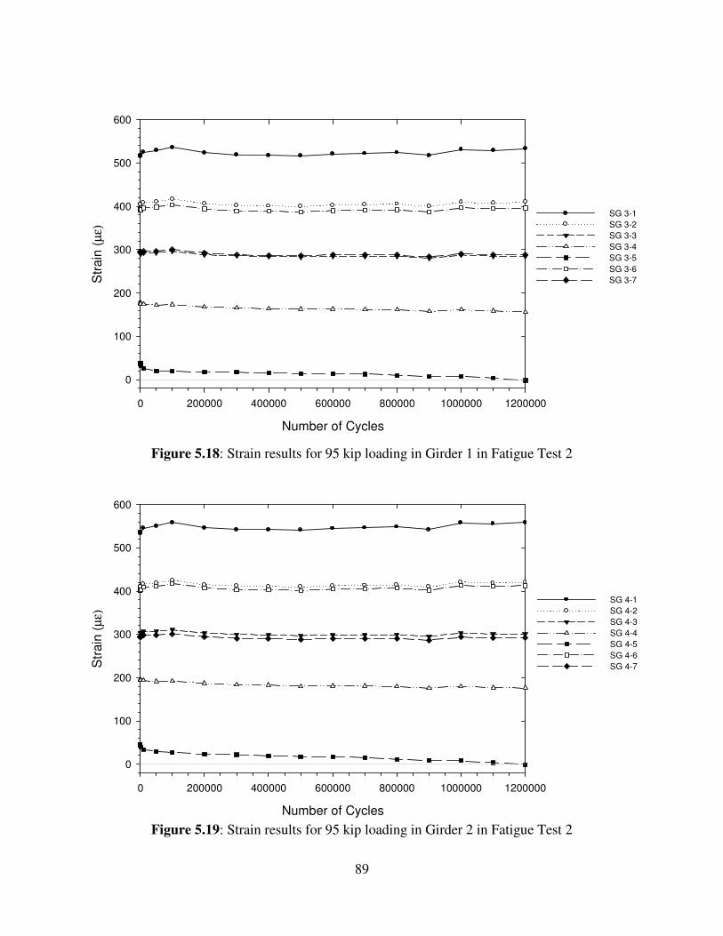
89

Number of Cycles

0 200000 400000 600000 800000 1000000 1200000

Str

ain

(µ

ε)

0

100

200

300

400

500

600

SG 3-1

SG 3-2

SG 3-3

SG 3-4

SG 3-5

SG 3-6

SG 3-7


Number of Cycles

0 200000 400000 600000 800000 1000000 1200000

Str

ain

(µ

ε)

0

100

200

300

400

500

600

SG 4-1

SG 4-2

SG 4-3

SG 4-4

SG 4-5

SG 4-6

SG 4-7


90

As with Fatigue Test 1, the change in strain during Fatigue Test 2 was minimal. The

plots indicate that the change in strain was approximately linear over the course of the test, with

the trends at each location on Girder 1 matching almost exactly their counterparts from Girder 2.

In general, the values of the strains at the top of Girder 2 were slightly less than those from

Girder 1 and the strains at the bottom of Girder 2 were slightly larger than those in Girder 1,

which can be accounted for by the conclusion that Girder 2 is taking more of the load than Girder

1. However, the percentage change from initial for all locations was approximately the same for

both girders, indicating similar amounts of damage to each system.

The point about which the strains below increase and the strains above decrease appears

to be between gauges 2 and 3 in Girder 1 and at gauge 3 in Girder 2. The flaring out about these

points in the plots indicates an overall increase in curvature shown in Figs. 5.20 and 5.21, which

suggests a loss of composite action leading to a reduction in stiffness resulting from increased

slip at the interface which causes an increase in deflection, which agrees with the vertical

deflection results. In examining the strain plots (Figs. 5.18 and 5.19), there are two points at

which jumps in the strain values become apparent. The first occurs between 100,000 and

200,000 cycles, where before the flaring of the strains indicated a rapid increase in curvature

which suddenly decreases at 200,000 cycles. This reduction in curvature represents a leveling

off or decrease in vertical deflection, which was observed in the vertical deflection results. It is

believed that the decrease in curvature was caused by the stabilization of the system resulting

from the settling of the test specimen, which agrees with vertical deflection, slip, and elastic

neutral axis (ENA) results. A similar jump occurs between 900,000 and 1,000,000 cycles.

However, the jump here caused the curvature to increase, which matches the increase in vertical

deflections and downward movement of the ENA. When the strains begin to level out and

rebound to previous values, so do the vertical deflections in both girders. As noted previously,

neither jump is large enough to indicate that any significant damage has been inflicted on the

system, such as the fracture of a shear stud.

91

Strain (µε)

0 100 200 300 400 500 600

Ve

rtic

al Lo

ca

tio

n (

in.)

0

5

10

15

20

25




Figure 5.20: Vertical strain distribution at 95 kips in Girder 1 at start and end of Fatigue Test 2

Strain (µε)

0 100 200 300 400 500 600

Vert

ical Loca

tion

(in

.)

0

5

10

15

20

25




Figure 5.21: Vertical strain distribution at 95 kips in Girder 2 at start and end of Fatigue Test 2

92

The increase in curvature, and subsequently the increase in deflections, is also reflected

in the movement of the elastic neutral axis (ENA) of the steel girder toward the bottom of the

section, shown in Figure 5.22. The ENA was calculated the same way as it was in Fatigue Test

1, by fitting a least squares linear regression line to the strain distribution in the girder cross-

section and then finding where that line crosses the zero strain line. As with Fatigue Test 1, the

calculated ENA for the test specimen from both girders fell between the upper bound (fully

composite) of 25.1 in. and the lower bound (no interaction) ENA of 10.4 in., as measured from

the bottom of the section, for the entirety of the test. This indicates a partial composite system,

as expected. The ENA dropped rapidly (relatively) in the first 100,000 cycles for both girders as

the test specimen settled; however after this point in the testing it leveled out and then

approached the bottom of the section at approximately linearly for each girder. The rate of

downward movement of the ENA in Girder 2 was slightly greater than that of Girder 1, as

evidenced by the closing of the gap between the two lines, which correlates well with slip data

reported, with the slip values in Girder 2 increasing faster than their counterparts in Girder 1.


0 200000 400000 600000 800000 1000000 1200000

Ne

utr

al A

xis

Lo

ca

tio

n (

in.)

0

5

10

15

20

25




Figure 5.22: Steel girder elastic neutral axis from bottom of section Fatigue Test 2

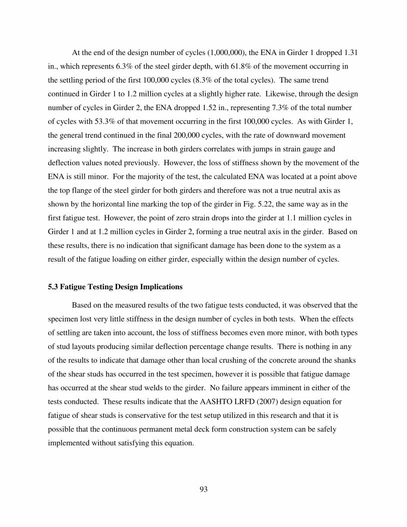
93

At the end of the design number of cycles (1,000,000), the ENA in Girder 1 dropped 1.31

in., which represents 6.3% of the steel girder depth, with 61.8% of the movement occurring in

the settling period of the first 100,000 cycles (8.3% of the total cycles). The same trend

continued in Girder 1 to 1.2 million cycles at a slightly higher rate. Likewise, through the design

number of cycles in Girder 2, the ENA dropped 1.52 in., representing 7.3% of the total number

of cycles with 53.3% of that movement occurring in the first 100,000 cycles. As with Girder 1,

the general trend continued in the final 200,000 cycles, with the rate of downward movement

increasing slightly. The increase in both girders correlates with jumps in strain gauge and

deflection values noted previously. However, the loss of stiffness shown by the movement of the

ENA is still minor. For the majority of the test, the calculated ENA was located at a point above

the top flange of the steel girder for both girders and therefore was not a true neutral axis as

shown by the horizontal line marking the top of the girder in Fig. 5.22, the same way as in the

first fatigue test. However, the point of zero strain drops into the girder at 1.1 million cycles in

Girder 1 and at 1.2 million cycles in Girder 2, forming a true neutral axis in the girder. Based on

these results, there is no indication that significant damage has been done to the system as a

result of the fatigue loading on either girder, especially within the design number of cycles.

5.3 Fatigue Testing Design Implications

Based on the measured results of the two fatigue tests conducted, it was observed that the

specimen lost very little stiffness in the design number of cycles in both tests. When the effects

of settling are taken into account, the loss of stiffness becomes even more minor, with both types

of stud layouts producing similar deflection percentage change results. There is nothing in any

of the results to indicate that damage other than local crushing of the concrete around the shanks

of the shear studs has occurred in the test specimen, however it is possible that fatigue damage

has occurred at the shear stud welds to the girder. No failure appears imminent in either of the

tests conducted. These results indicate that the AASHTO LRFD (2007) design equation for

fatigue of shear studs is conservative for the test setup utilized in this research and that it is

possible that the continuous permanent metal deck form construction system can be safely

implemented without satisfying this equation.

94

5.4 Summary of Laboratory Fatigue Testing

A full-scale steel-concrete composite girder bridge test specimen was constructed

utilizing the continuous permanent metal deck form construction method. The specimen was

constructed with two different stud layouts on each half of the bridge, with the near half

containing one stud-per-rib and the far side containing two studs-per-rib. However, due to the

limited number of ribs available using this construction method, AASHTO LRFD (2007)

provisions for fatigue resistance could not be met. Therefore, two fatigue tests were conducted

on the test specimen, one at the near side quarter point and another at the far side quarter point,

to determine the fatigue resistance of each stud layout as compared with the AASHTO fatigue

equation (Eqs. 2.21-2.23). The specimen was loaded cyclically to a load range calculated based

on this equation to cause failure at 1,000,000 cycles. A separate load range was calculated for

each of the tests because of the different section properties that arise from have two different

numbers of studs per rib. The specimen was subjected to 1,200,000 cycles in each test. The

fatigue resistance of the specimen was to be tracked by measuring the loss of stiffness over the

course of the testing.

Various types of measurements were taken during testing, including vertical deflections

at the point of loading and mid-span, strain in the cross-section at the point of loading, and slip

between the steel girder and concrete deck. These readings were used to track the loss of

stiffness of the section over the duration of each test to tell us if there was any loss of composite

action between the steel girder and concrete deck. A summary of the results through the design

number of cycles (1,000,000) is provided in Table 5.3.

Table 5.3: Summary of laboratory fatigue testing

Initial Final % Change Initial Final % Change Initial Final % Change

FT 1 - Girder 1 -0.115 -0.120 4.53% 22.4 21.6 -3.44% -0.0011 -0.0013 18.2%

FT 1 - Girder 2 -0.115 -0.121 5.41% 22.2 21.3 -4.19% -0.0013 -0.0022 69.2%

FT 2 - Girder 1 -0.211 -0.225 6.70% 22.2 20.9 -5.90% -0.0019 -0.0048 153%

FT 2 - Girder 2 -0.217 -0.237 9.41% 22.6 21.0 -6.74% -0.0025 -0.0054 116%

Neutral Axis (in. from bottom)Deflection at Point of Load (in.) End of Span Slip (in.)Test

As can be seen in Table 5.3, the specimen performed very well during both of the fatigue

tests, losing very little stiffness and with no apparent shear stud failures occurring. The

percentage change in deflection of the specimen was slightly greater in Fatigue Test 2 than in

95

Fatigue Test 1, a fact which agrees with the neutral axis and slip results. It is important to note

that both tests exhibited a settling period lasting 50,000 cycles in Test 1 and 100,000 cycles in

Test 2. This settling period accounted for a large amount of the increase in deflections in Test 2

and therefore the fatigue resistance of the far side of the bridge is higher than it seems. This

effect was observed to a lesser degree in Test 1. Similar patterns in the results were observed in

both tests in the 200,000 cycles loaded beyond the design number of cycles, telling us that failure

was not imminent in either test. This conclusion is supported by the analysis where the

deflections were extrapolated to five million cycles assuming the same linear trend. One aspect

of Table 5.3 that stands out are the very high values for percentage change in slip for the fatigue

tests, especially in Fatigue Test 2. It is important to point out that the values for slip are very

small and even minute increases in slip would result in large percentage changes. Therefore, the

large percent changes are not indicative of major damage to the test specimen and should only be

considered while taking into account the size of the slip values.

Based on the results presented, it can be concluded that there was no significant damage

done to the test specimen as result of the loads cycles applied in either test. Therefore, it can be

concluded that the AASTHO LRFD (2007) fatigue equation produced very conservative results

for the test specimen as it was designed to fail at one million cycles.

96

Chapter 6: Laboratory Static Testing Results

6.1 Near Side Test in Elastic Region (Static Test 1)

Test 1 was conducted at the quarter point in the near half of the test specimen as a means

of gathering data on the one stud-per-rib geometry in the elastic region while not causing damage

to the specimen that would affect the test to failure on the far half of the bridge (Test 2). Both

girders were loaded to 65 kips, which is approximately 40% of the calculated moment capacity

of the section, to ensure that the specimen remained in the linear elastic region so that no

significant damage would be done to the specimen.

Static Test 1 went exactly as planned, with no problems being encountered. As can be

seen in the plot of the moment deflection curve produced for the point of loading location, given

in Figure 6.1, the responses for both girders remained almost perfectly linear during the loading

period. The unload for the test is not quite as linear; however the deflection values for both

girders returned to approximately -0.004 in. at zero load, which represents about 0.2% of the

largest deflection achieved in the test. Therefore, it was concluded that that the desired elastic

response was achieved in this test and that no damage was done to the specimen. One other

important conclusion that can be drawn from Test 1 is that measured deflections of both girders

were less than the predicted deflections using the AISC effective moment of inertia equation (Eq.

2.15). The deflection values calculated using the full effective moment of inertia (without the

0.75 reduction factor applied) were a better predictor of the measured deflections.

Measurements for slip were taken during Test 1, however they are not going to be reported

because they hold little value with regards to the scope of this test. Slip values were linear for

the entire loading period and all returned to zero following unload, indicating no damage as

result of testing.

The deflection values reported in Fig. 6.1 have been adjusted to account for both bearing

pad compression and rotation at supports. This was done by first taking the girder deflection

values measured on either side of each bearing location and averaging them to produce a

compression and rotation adjusted support deflection. Once the values for all of the support

deflections were known, the values for the deflections at the point of loading were calculated in

the same way as they were in the fatigue tests. The effects of support deflection were taken into

account by subtracting the deflection of the support farthest from the point of loading from the

97

deflection of the support closest to the point of loading and then multiplying that by 0.75 to

account for the location in the span. This value was then added to the deflection of the support

farthest from the point of loading and then that total value was subtracted from the measured

deflection at the point of loading to get the final reported deflection (absolute deflection).

∆ (in.)

0.00 0.05 0.10 0.15 0.20 0.25 0.30 0.35

Mm

(ft

-kip

s)

0

50

100

150

200

250

300

350

400

Test 1 - Girder 1

Test 1 - Girder 2

Calculated Elastic Stiffness - 100% Ieff


Figure 6.1: Static Test 1 point of loading measured moment versus deflection

One other conclusion that can be drawn from the moment-deflection results of Static Test

1 is that the measured elastic deflections for the test specimen were less than the calculated

values of the elastic deflections using both the full value of the AISC effective moment of inertia

(Ieff) and the recommended reduced value of 0.75. The predicted deflections using the unreduced

value of Ieff were significantly closer to the measured values than the reduced values; however

the reduced Ieff produced more conservative results.

98

6.2 Far Side Static Test to Failure (Static Test 2)

6.2.1 Overview

Static Test 2 was conducted at the far side quarter point to determine the plastic capacity

of the test specimen with the two studs per rib geometry. The test was run over eight hours until

a total deflection of 2.75 in. was reached, at which point it was concluded that the plastic

moment of the system had been achieved because the load-deflection curve had leveled off. It

was decided that any additional load could cause enough damage to adversely affect the strength

of the near half of the specimen, which was to be tested next, and therefore loading was stopped

and the specimen unloaded.

Only one problem was encountered during Static Test 2. At approximately 1.5 in. of total

deflection, the rotation in the hinge being formed at the point of loading in the test specimen

became so large that the bottom of the concrete deck came into contact with the shaft of the

linear variable displacement transducer (LVDT) being used to measure interface slip at that

location on both girders. This caused a bias in the measurements being taken by those sensors so

that the data taken no longer accurately represented the actual specimen response. Also, the deck

pressing against the sensor shaft caused a moment in the sensor that, as the rotation got large and

larger, could have potentially damaged the sensor. Therefore, it was decided at this point to

remove the sensors. A new LVDT mounting system was put in place for Static Test 3 to prevent

this from happening in the next test. No other problems were encountered during Test 2.

Figure 6.2: Examples of shear stud failures at the end of Static Test 2

From examining the test specimen before, during, and after the Test 2, it became obvious

that the main failure mode for the shear studs was the tearing of the stud through the web of the

ribs of the profiled steel deck form, which supports the assumption of weak side stud position.

99

Three different examples of this failure are shown in Fig. 6.2. The first picture shows the rib

immediately after rupture, before the shear stud had broken out too far. The second image shows

the blowout after the shear stud had pushed out far enough to deform the steel deck and cause

some cracking in the concrete. The third picture in Fig. 6.2 shows the rib blowout after the shear

studs had pushed out far enough to cause major damage to the rib location, as indicated by the

significant cracking of the surrounding concrete. These blowouts were first noticed at a total

deflection of about 2 in. in the ribs closest to the end of the span. As the test continued, more

and more blowouts occurred, with each failure marked by a distinct high-pitched “pinging”

noise. The locations of each of the blowouts in the shear span being tested are shown in Fig. 6.3,

with blowouts being indicated by an “X” going through that rib location. No blowouts or

bulging was observed in the mid-span side of loading. There does not appear to be any pattern

with regard to the sections where blowouts occurred, which tells us that where the blowouts

happened may have been weak links in the system. These weak links could have been the result

of the shear stud being placed off center in the rib bottom flange, which would result in there

being less concrete between the stud shank and the rib web if the stud placement was biased

toward the point of maximum moment. The point where no blowouts occurred could also be the

result of the shear stud rupturing, however this is unlikely. It is important to note that at every

location where the steel deck did not rupture, there was still bulging in the web of the rib, which

leads to the conclusion that if the test had continued, these locations would have pushed through

the rib web eventually, assuming that the shear stud had not ruptured. This assumption is

supported by the Static Test 3 failures described in later sections.

1 2 3 5 84 6 7 9 10 11

Center ofBearing

Point ofLoading

Girder 2

Girder 1

Figure 6.3: Shear stud blowout locations at the end of Static Test 2

100

Major damage was also done to both the steel girders and concrete deck. At the end of

Test 2, it was very obvious that a plastic hinge had formed in the steel girder by examining the

Luder Lines formed in the whitewash at the point of loading, as shown first in Fig. 6.4. The

presence of the Luder Lines verifies that the steel section has yielded in this area, which is

desired in achieving the plastic moment of the specimen. With regards to the concrete deck,

significant cracking occurred over the course of the test, shown in the second image in Fig. 6.4.

As can be seen, the largest of the cracks travel most of the way up the depth of the deck, telling

us that very little of the deck is in compression, as expected at the plastic moment, and also that

by the end of the test the specimen was acting almost like two separate bodies on either side of

the loading point. Similar damage was noted in both girders. Therefore, based on the visual

results, it is believed that the plastic moment of the section was achieved.

Figure 6.4: Specimen damage in girders and deck at the end of Static Test 2

One other interesting indication of damage to the system was located on the bottom of the

top flange just below where shear studs had been welded. At these locations, there are

indications that yielding had occurred in the top flange of the girders that were localized to where

the shear studs had been welded as signified by the circular patterns of flaking that formed in the

whitewash at lower levels of deflection, shown in Fig. 6.5. The first image shows the pattern

formed at the first point this phenomenon was noticed while the second image shows the flake

pattern at the end of testing, showing a progression of this yield across the top flange. These

yield patterns only occurred below studs in the shear span, not in the mid-span side of the

loading. It is not known how far toward the end of the span this was happening because the

whitewash only extended to three feet on either side of the point of loading, however this could

be indicative of a failure mode of the shear studs and therefore warrants further investigation.

101

Figure 6.5: Localized top flange yielding under shear studs

6.2.2 Moment and Deflection Results

This section discusses the moment and deflection results of Static Test 2. The moment

results presented here come from a direct calculation using the loads recorded in the load cells

above the hydraulic jacks for each girder assuming a simply supported beam with a quarter point

loading. The deflections presented here have been adjusted to account for compression of the

neoprene bearing pads and rotation at the supports as described in the Static Test 1 results

previously. The moment and deflection results of Test 2 are shown plotted in Fig. 6.6. As can

be seen, the responses of both girders are almost identical, with the moment and deflection

values for Girder 2 being just slightly greater than Girder 1 until the unload period. Both girders

exhibited a nearly linear response, with very few jumps or inconsistencies, until a moment of

approximately 700 ft-kips was reached at a deflection of around 0.6 in. at which point the

specimen began to exhibit non-linear behavior, as evidenced by the leveling off of the plots. The

specimen reached a plateau at a moment of about 980 ft-kips per girder, at which point the

applied moment rose very little with the increases in deflection for the remainder of the test,

indicating that the plastic moment capacity had been reached in each girder. The specimen was

unloaded at an adjusted deflection of 2.54 in. in Girder 1 and 2.58 in. in Girder 2. Both girders

followed a similar unload response which will be discussed in further detail later in this section.

The measured moment strengths of both girders were well below the calculated moment

capacity (Mc) of 1150 ft-kips, illustrated in Fig. 6.6 by the horizontal dotted line. The maximum

moment attained in Girder 1 was 984 ft-kips, which is 14.3% lower than the calculated moment

capacity. Similarly, Girder 2 reached a maximum moment of 989 ft-kips, which is 13.9% lower

than the calculated moment capacity. This leads to the conclusion that one or more elements of

the test specimen (i.e. shear studs, steel girder, steel deck formwork, concrete deck) did not

102

perform as predicted in the calculation of plastic moment capacity. It is believed that the shear

studs did not reach their full calculated capacities before tearing through the rib webs as shown

in the “Overview” section, which would account for both the lower than expected measured

plastic moment and the plastic neutral axis being located closer to the bottom of the section than

expected, as discussed in the “Strain Results” section to follow.

∆ (in.)

0.0 0.5 1.0 1.5 2.0 2.5 3.0

Mm

(ft

-kip

s)

0

100

200

300

400

500

600

700

800

900

1000

1100

1200

Test 2 (Far) - Girder 1


Calculated Moment Capacity (Mc)



Calculated Non-Composite Strength

Figure 6.6: Test 2 point of loading measured moment versus deflection

Another important conclusion that can be drawn from examining the moment-deflection

results of Test 2 deals with what value of the AISC commentary provisions (2005) for the

effective moment of inertia (Ieff) most accurately predicts the elastic response of the test

specimen. When looking at the test specimen response in Fig. 6.6, it is obvious that the

deflections in the linear-elastic region of the test specimen, from 0 to about 700 ft-kips per

girder, are less than the predicted elastic deflections calculated using both 75% (recommended)

103

and 100% of the Ieff based on a non-prismatic section. These elastic deflections are shown in

Figure 6.6 by the dotted diagonal lines. The deflection values calculated using the unreduced Ieff

are just slightly greater than the measured deflections in the elastic region and therefore are much

closer to the measured deflections than the 75% Ieff deflection values. What is important is that

the unreduced effective moment of inertia provides an accurate prediction of the actual response

without overestimating the stiffness of the specimen, thereby producing a conservative value.

One other significant aspect of the Test 2 results is the unload response of the test

specimen. The unload response for both girders is nearly linear until a moment of approximately

600 ft-kips is reached, at which point the response becomes non-linear with decreasing stiffness.

The linear portion of the unload response runs parallel to the elastic loading portion of the test. It

is believed that the specimen began to exhibit a non-linear response at 600 ft-kips because this is

the point at which the shear studs lost contact with the concrete surrounding them. As the shear

studs begin to disengage from the concrete, the specimen becomes softer due to a lack of

compression, which would alter the response. Also, the point of change from linear to non-linear

correlates almost exactly with the point at which the slip response in the unload changes from

linear to non-linear as shown in the “Slip Results” section, which lends support to this

conclusion.


This section contains the results and analysis of the strain gauge data taken during Static

Test 2. The strain data taken during this test was used primarily for the determination of the

plastic neutral axis for both girders during the test. The neutral axis of the steel girder for the

static test to failure was calculated the same way as it was in the fatigue tests. A least squares

linear regression line was fit to the measured vertical strain distribution of the girder cross-

section and the neutral axis is calculated as the vertical location where the regression line crosses

the zero strain line (the Y-axis in this case). As with the fatigue tests, the values of strain gauges

at locations 2 and 6 were averaged as well as locations 3 and 7 to account for out of plane

bending in the girders. However, the calculation of the neutral axis presented many challenges

in the static tests conducted as part of this research. Due to the high strains induced by the large

deflections in the specimen and the fact that the bond was already weak from the load cycles

applied during the fatigue testing, it was not uncommon for individual strain gauges to become

104

debonded from the steel and produce values that did not make sense given the overall strain

distribution being produced by all the gauges. To correct for this, strain distributions were

plotted for every data point taken during the static test so that it could be determined when

individual strain gauges began to produce strains that did not match the overall distribution, as

indicated by values that did not follow the approximately straight line that was expected. At the

point where non-linear values were being produced by a strain gauge, the values for that gauge

were removed from the linear regression analysis for the remainder of the data points so that they

would not skew the subsequent neutral axis results. This process was applied to the strain values

produced by both girders in the test. To assure accuracy of results, at least three strain gauge

locations were used to fit the line that determined the neutral axis location. The neutral axis was

no longer calculated when the point was reached where data from three good gauges was no

longer possible. The typical progression of gauge failure started with the gauge at the bottom of

the section (location 1) followed by the next higher gauge and so on up the section.

The results of the calculation of the neutral axis with respect to the applied moment in

Static Test 2 are presented in Fig. 6.7. The neutral axes for both girders are almost identical for

the entirety of the test, following the exact same trends. In examining the plot below, the plastic

neutral axis is taken as the point where the curve is approximately vertical, which says that as the

moment in the section increases there is no change in the neutral axis location indicating

stabilization in the composite system. There are two locations in the results where the curve is

approximately vertical. The first occurs at lower moments before non-linear behavior of the

specimen is reached and therefore this is the location of the elastic neutral axis. The second time

the curve is almost vertical occurs at higher loads and is indicated by dotted vertical lines for

each girder. The location of the plastic neutral axis (PNA) is taken as 18.3 in. from the bottom of

the section for Girder 1and 18.2 in. from the bottom of the section for Girder 2. Both of these

values are about 2 in. less than the predicted PNA location of 20.285 in. from the bottom of the

section found in the calculation of the plastic moment capacity (see Appendix G).

The difference between the calculated and measured PNA can be explained by the

capacity of the individual shear studs in the test specimen being less than the predicted capacity.

If the capacity of the shear studs is lower than expected in the specimen, this means that less

force is being transferred horizontally at the interface between the concrete deck and the steel

girder and therefore the compressive force in the concrete deck will be reduced. The overall

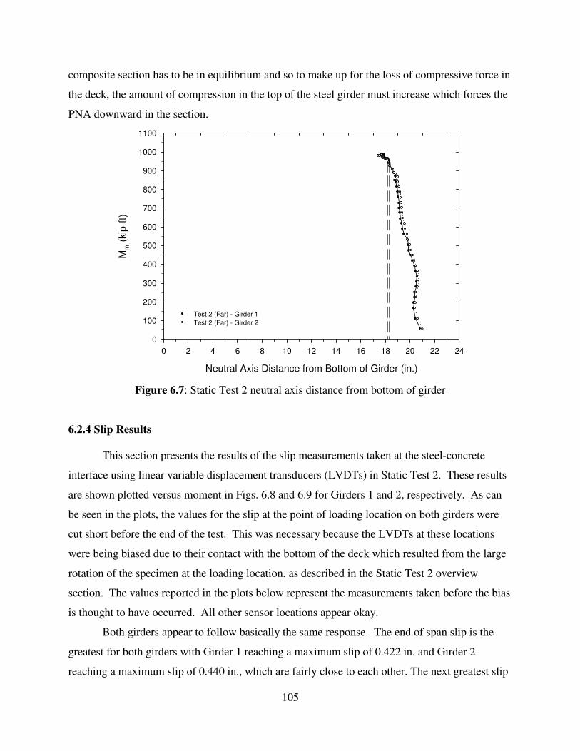
105

composite section has to be in equilibrium and so to make up for the loss of compressive force in

the deck, the amount of compression in the top of the steel girder must increase which forces the

PNA downward in the section.

Neutral Axis Distance from Bottom of Girder (in.)

0 2 4 6 8 10 12 14 16 18 20 22 24

Mm

(kip

-ft)

0

100

200

300

400

500

600

700

800

900

1000

1100



Figure 6.7: Static Test 2 neutral axis distance from bottom of girder

6.2.4 Slip Results

This section presents the results of the slip measurements taken at the steel-concrete

interface using linear variable displacement transducers (LVDTs) in Static Test 2. These results

are shown plotted versus moment in Figs. 6.8 and 6.9 for Girders 1 and 2, respectively. As can

be seen in the plots, the values for the slip at the point of loading location on both girders were

cut short before the end of the test. This was necessary because the LVDTs at these locations

were being biased due to their contact with the bottom of the deck which resulted from the large

rotation of the specimen at the loading location, as described in the Static Test 2 overview

section. The values reported in the plots below represent the measurements taken before the bias

is thought to have occurred. All other sensor locations appear okay.

Both girders appear to follow basically the same response. The end of span slip is the

greatest for both girders with Girder 1 reaching a maximum slip of 0.422 in. and Girder 2

reaching a maximum slip of 0.440 in., which are fairly close to each other. The next greatest slip

106

was at the mid-shear span location followed by the lowest slip at the point of loading within the

values reported. The response of the slip at the end of the span was linear until approximately

400 ft-kips on both girders while the response at the other two locations remained linear until

about 850 ft-kips. This early shift in from linear to non linear behavior can be explained by the

fact that the shear studs at the end of the span tend to receive more of the horizontal shear load

than those more in the interior of the shear span. Therefore, because the load on the shear studs

at the end is greater, there tends to be more slip and the onset of inelastic behavior comes sooner

as damage is done to the ribs at the end of the span. The biggest difference between the response

of Girder 1 and that of Girder 2 is that the slip at the mid-shear span location of Girder 1 is

significantly lower than Girder 2. Both girders were following almost the exact same path at this

sensor location until a slip of 0.142 in. was reached in Girder 1, at which point the slip jump up

suddenly and then stopped increasing for the remainder of the test until unloading. It is unlikely

that this discrepancy resulted from a change in the test specimen because the end of span

response does not follow the same trend. Therefore, it has been concluded that this is most likely

the result of something affecting the LVDT, similarly to what happened at the point of loading

sensor location. The entirety of the test data was plotted for the malfunctioning LVDT so that

the unload response could be shown. Girder 2 data from the mid-shear span location is assumed

to be good and tells us that the slip at this location is just slightly less than that at the end of the

span, reaching a maximum slip of 0.390 in.

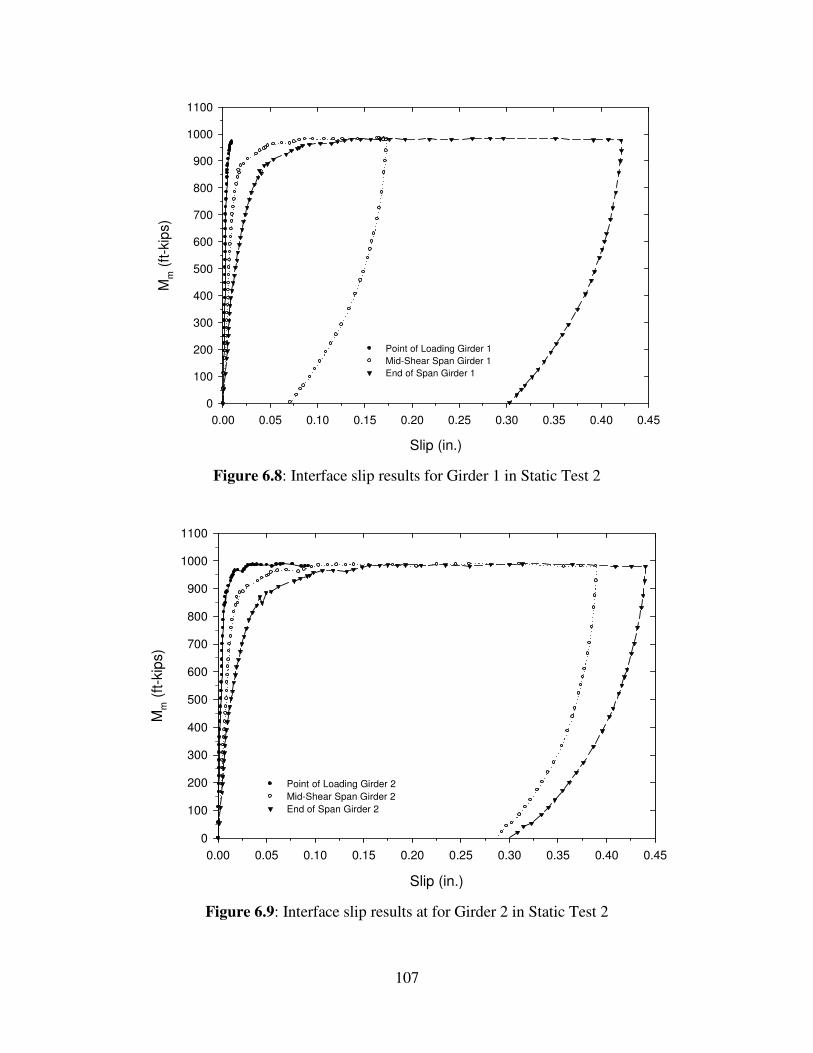
107

Slip (in.)

0.00 0.05 0.10 0.15 0.20 0.25 0.30 0.35 0.40 0.45

Mm

(ft

-kip

s)

0

100

200

300

400

500

600

700

800

900

1000

1100

Point of Loading Girder 1

Mid-Shear Span Girder 1

End of Span Girder 1

Figure 6.8: Interface slip results for Girder 1 in Static Test 2

Slip (in.)

0.00 0.05 0.10 0.15 0.20 0.25 0.30 0.35 0.40 0.45

Mm

(ft

-kip

s)

0

100

200

300

400

500

600

700

800

900

1000

1100




Figure 6.9: Interface slip results at for Girder 2 in Static Test 2

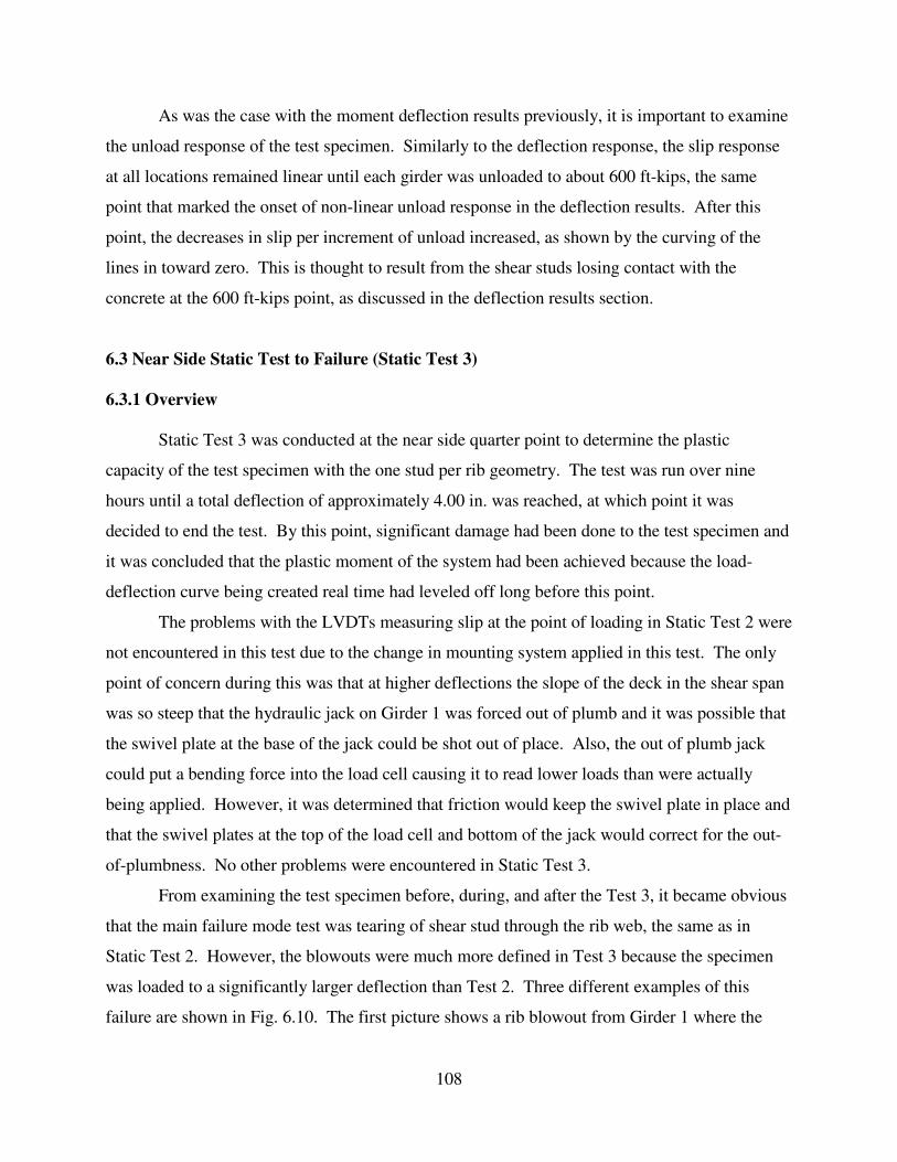
108

As was the case with the moment deflection results previously, it is important to examine

the unload response of the test specimen. Similarly to the deflection response, the slip response

at all locations remained linear until each girder was unloaded to about 600 ft-kips, the same

point that marked the onset of non-linear unload response in the deflection results. After this

point, the decreases in slip per increment of unload increased, as shown by the curving of the

lines in toward zero. This is thought to result from the shear studs losing contact with the

concrete at the 600 ft-kips point, as discussed in the deflection results section.

6.3 Near Side Static Test to Failure (Static Test 3)

6.3.1 Overview

Static Test 3 was conducted at the near side quarter point to determine the plastic

capacity of the test specimen with the one stud per rib geometry. The test was run over nine

hours until a total deflection of approximately 4.00 in. was reached, at which point it was

decided to end the test. By this point, significant damage had been done to the test specimen and

it was concluded that the plastic moment of the system had been achieved because the load-

deflection curve being created real time had leveled off long before this point.

The problems with the LVDTs measuring slip at the point of loading in Static Test 2 were

not encountered in this test due to the change in mounting system applied in this test. The only

point of concern during this was that at higher deflections the slope of the deck in the shear span

was so steep that the hydraulic jack on Girder 1 was forced out of plumb and it was possible that

the swivel plate at the base of the jack could be shot out of place. Also, the out of plumb jack

could put a bending force into the load cell causing it to read lower loads than were actually

being applied. However, it was determined that friction would keep the swivel plate in place and

that the swivel plates at the top of the load cell and bottom of the jack would correct for the out-

of-plumbness. No other problems were encountered in Static Test 3.

From examining the test specimen before, during, and after the Test 3, it became obvious

that the main failure mode test was tearing of shear stud through the rib web, the same as in

Static Test 2. However, the blowouts were much more defined in Test 3 because the specimen

was loaded to a significantly larger deflection than Test 2. Three different examples of this

failure are shown in Fig. 6.10. The first picture shows a rib blowout from Girder 1 where the

109

concrete between the rib web and the shear stud completely crushed. The second image shows a

blowout example at one of the deck sheet overlap points, which is interesting because only the

deck section on the bottom ruptured while the web part of the overlap stayed intact. This

indicates that the rupture more than likely initiates at imperfections in the steel deck that result

from the welding of the shear stud. The third picture in Fig. 6.10 shows a rib blowout from

Girder 2 where the concrete in the rib has significant cracking. These blowouts were first

noticed at a total deflection of about 1.75 in. in the ribs closest to the end of the span with the

blowouts increasing in the shear span as the test continued. The same high-pitched “pinging”

noise was observed at the point of steel rupture as in Test 2. The locations of each of the

blowouts in the shear span being tested are shown in Fig. 6.11, with blowouts being indicated by

an “X” going through that rib location. As can be seen, blowouts and rupture of the cold form

steel deck ribs occurred at every rib location in the shear span except for the ribs closest to the

point of loading, where the slip is limited by the large amounts of friction at the interface due to

the nearby loading. This supports the conclusion reached in Test 2 that blowouts would have

occurred at almost every rib in the shear span in that test if loading had not been stopped. No

blowouts or bulging were observed in the mid-span side of loading.

Figure 6.10: Examples of shear stud failures at the end of Static Test 3

110

12358 46791011

Center ofBearing

Point ofLoading

Girder 2

Girder 1

12

Figure 6.11: Shear stud blowout locations at the end of Static Test 3

Significant damage was also done to both the steel girders and concrete deck. At the end

of Test 3, it was very obvious that a plastic hinge had formed in the steel girder by observing the

Luder Lines formed in the whitewash at the point of loading that formed 45̊ angles with the

respect to the bottom of the section, as shown first in Fig. 6.12. Vertical lines in the whitewash

near the top of both girders on either side of the point of loading also indicate that compression

yielding has occurred in that area. The presence of the Luder Lines and compression yielding

lines verifies that the steel section has yielded in this area, which is desired in achieving the

plastic moment of the specimen. It also appears that the top flange has buckled under the

compression load, as seen in the second picture in Fig. 6.12. With regards to the concrete deck,

significant cracking occurred over the course of the test. As was the case in Test 2, the largest of

the cracks traveled most of the way up the depth of the deck, telling us that very little of the deck

is in compression, as was expected at the plastic moment, and also that by the end of the test the

specimen was acting almost like two separate bodies on either side of the loading point, the same

as in Static Test 2. Similar damage was observed in both girders. Therefore, based on the visual

results, it is believed that the plastic moment of the section was achieved. Figure 6.13 provides

some general images of the specimen at the end of testing.

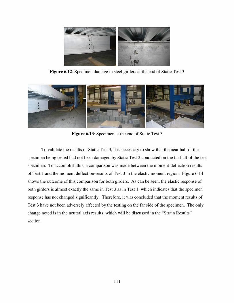
111

Figure 6.12: Specimen damage in steel girders at the end of Static Test 3

Figure 6.13: Specimen at the end of Static Test 3

To validate the results of Static Test 3, it is necessary to show that the near half of the

specimen being tested had not been damaged by Static Test 2 conducted on the far half of the test

specimen. To accomplish this, a comparison was made between the moment-deflection results

of Test 1 and the moment deflection-results of Test 3 in the elastic moment region. Figure 6.14

shows the outcome of this comparison for both girders. As can be seen, the elastic response of

both girders is almost exactly the same in Test 3 as in Test 1, which indicates that the specimen

response has not changed significantly. Therefore, it was concluded that the moment results of

Test 3 have not been adversely affected by the testing on the far side of the specimen. The only

change noted is in the neutral axis results, which will be discussed in the “Strain Results”

section.

112

∆ (in.)

0.0 0.1 0.2 0.3 0.4 0.5

Mm

(ft

-kip

s)

0

100

200

300

400

500

600

Test 1 - Girder 1

Test 3 - Girder 1

∆ (in.)

0.0 0.1 0.2 0.3 0.4 0.5M

m (

ft-k

ips)

0

100

200

300

400

500

600

Test 1 - Girder 2

Test 3 - Girder 2

Figure 6.14: Comparison of measured elastic deflections of Static Test 1 to Static Test 3

6.3.2 Moment and Deflection Results

This section discusses the moment and deflection results from Static Test 3. As with

Static Tests 1 and 2, the moment results presented here come from a direct calculation using the

loads recorded in the load cells above each hydraulic jack for each girder assuming a simply

supported beam with a quarter point loading. The deflections given here have been adjusted to

account for compression of the neoprene bearing pads and rotation at the supports as described in

the Static Test 1 results. The moment and deflection results of Test 3 are shown plotted in Fig.

6.15. As can be seen, the response of both girders is almost exactly the same, with the moment

and deflection values for Girder 1 being just slightly greater than Girder 2 for almost the entirety

of the test. Both girders exhibited a nearly identical linear response, with very few jumps or

inconsistencies, until a moment of approximately 510 ft-kips was reached at a deflection of

around 0.44 in. at which point the specimen began to exhibit non-linear behavior, as evidenced

by the leveling off of the curve. The specimen continued to take load with increasing deflections

until it reached a plateau at a moment of about 860 ft-kips per girder, at which point the applied

moment rose very little with the increases in deflection for the remainder of the test, indicating

113

that the plastic moment capacity had been reached in each girder. The specimen was unloaded at

an adjusted deflection of 3.83 in. in Girder 1 and 3.80 in. in Girder 2. Both girders displayed a

similar unload response which will be discussed in further detail later in this section.

∆ (in.)

0.0 0.5 1.0 1.5 2.0 2.5 3.0 3.5 4.0

Mm

(ft

-kip

s)

0

100

200

300

400

500

600

700

800

900

1000

1100

Test 3 (Near) - Girder 1


Calculated Moment Capacity (Mc)



Calculated Moment Strength

Figure 6.15: Static Test 3 point of loading measured moment versus deflection

The measured plastic moment capacities of both girders were well below the calculated

moment capacity (Mc) of 960 ft-kips, illustrated in Fig. 6.15 by the horizontal dotted line. The

maximum moment attained in Girder 1 was 890 ft-kips, which is 7.3% lower than the calculated

moment capacity. The maximum moment reached in Girder 2 was slightly less than in Girder 1

at 879 ft-kips, which is 8.4% lower than the calculated moment capacity. It is important to note

that the maximum moments in this test were closer to the calculated values than the measured

plastic moments from Static Test 2. However, the same conclusion that that one or more

elements of the test specimen (i.e. shear studs, steel girder, steel deck formwork, concrete deck)

did not perform as predicted in the calculation of plastic moment capacity is still reached as in

Test 2.

114

The measured elastic deflections from Static Test 3 compares to the deflection values

calculated using the two levels of the AISC commentary provisions (2005) effective moment of

inertia equation (Ieff) exactly the same as in Static Test 2. As before, when examining the test

specimen response in Fig. 6.15, it is obvious that the deflections in the linear-elastic region of the

test specimen, from 0 to about 510 ft-kips per girder, are less than the predicted elastic

deflections calculated using both 75% (recommended) and 100% of the AISC effective moment

of inertia based on a non-prismatic section. These predicted elastic deflections are shown in Fig.

6.15 by the dotted diagonal lines. The deflection values calculated using the unreduced Ieff are

just slightly greater than the measured deflections in the elastic region and therefore are much

closer to the measured deflections than the 75% Ieff deflection values. What is important is that

the unreduced Ieff provides an accurate prediction of the actual response without overestimating

the stiffness of the specimen, thereby producing a slightly conservative deflection calculation.

The unload portion of this test presented a similar linear to non-linear response as Static

Test 2. The unload response for both girders is nearly linear until a moment of approximately

560 ft-kips is reached, at which point the plot begins to curve in toward zero, meaning that the

change of deflection per increment of moment is increasing. The linear portion of the unload

runs parallel to the elastic loading region of the curve, which tells us that specimen is initially

unloading elastically. This response as well at the slip results (presented in future sections) lead

to the same explanation of this behavior as in Test 2, which is that the moment of 560 ft-kips is

the point at which the shear studs break contact with the concrete it had been bearing against as

slip had been increasing and as the shear studs disengage from the concrete, the loss of the

compressive force leads to a softening of the system due to lack of composite action.


This section contains the results and analysis of the strain gauge data taken during Static

Test 3. The strain data taken during this test was used primarily for the determination of the

plastic neutral axis for both girders during the test. The calculation of the neutral axis of the steel

girder for this test followed the same procedure described in Static Test 2 and therefore will not

be repeated. The results of the calculation of the neutral axis with respect to the applied moment

in Test 3 are presented in Fig. 6.16 along with the neutral axis results from Static Test 1 to act as

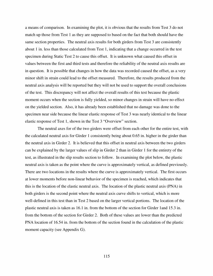
115

a means of comparison. In examining the plot, it is obvious that the results from Test 3 do not

match up those from Test 1 as they are supposed to based on the fact that both should have the

same section properties. The neutral axis results for both girders from Test 3 are consistently

about 1 in. less than those calculated from Test 1, indicating that a change occurred in the test

specimen during Static Test 2 to cause this offset. It is unknown what caused this offset in

values between the first and third tests and therefore the reliability of the neutral axis results are

in question. It is possible that changes in how the data was recorded caused the offset, as a very

minor shift in strain could lead to the offset measured. Therefore, the results produced from the

neutral axis analysis will be reported but they will not be used to support the overall conclusions

of the test. This discrepancy will not affect the overall results of this test because the plastic

moment occurs when the section is fully yielded, so minor changes in strain will have no effect

on the yielded section. Also, it has already been established that no damage was done to the

specimen near side because the linear elastic response of Test 3 was nearly identical to the linear

elastic response of Test 1, shown in the Test 3 “Overview” section.

The neutral axes for of the two girders were offset from each other for the entire test, with

the calculated neutral axis for Girder 1 consistently being about 0.65 in. higher in the girder than

the neutral axis in Girder 2. It is believed that this offset in neutral axis between the two girders

can be explained by the larger values of slip in Girder 2 than in Girder 1 for the entirety of the

test, as illustrated in the slip results section to follow. In examining the plot below, the plastic

neutral axis is taken as the point where the curve is approximately vertical, as defined previously.

There are two locations in the results where the curve is approximately vertical. The first occurs

at lower moments before non-linear behavior of the specimen is reached, which indicates that

this is the location of the elastic neutral axis. The location of the plastic neutral axis (PNA) in

both girders is the second point where the neutral axis curve shifts to vertical, which is more

well-defined in this test than in Test 2 based on the larger vertical portions. The location of the

plastic neutral axis is taken as 16.1 in. from the bottom of the section for Girder 1and 15.3 in.

from the bottom of the section for Girder 2. Both of these values are lower than the predicted

PNA location of 16.54 in. from the bottom of the section found in the calculation of the plastic

moment capacity (see Appendix G).

116

Neutral Axis Distance from Bottom of Section (in.)

0 2 4 6 8 10 12 14 16 18 20 22

Mm

(ft

-kip

s)

0

100

200

300

400

500

600

700

800

900

1000

Test 1 (Near Elastic) - Girder 1

Test 1 (Near Elastic) - Girder 2



Figure 6.16: Static Test 3 neutral axis distance from bottom of girder

6.3.4 Slip Results

This section presents the results of the slip measurements taken at the steel-concrete

interface using linear variable displacement transducers (LVDTs) in Static Test 3. These results

are shown plotted versus moment in Figs. 6.17 and 6.18 for Girders 1 and 2, respectively. As

can be seen in Fig. 6.18, the value for the slip at the point of loading location on Girder 2 was cut

short well before the end of the test due to an unexplained bias on the sensor. The values

reported in the plots below represent the measurements taken before the bias is thought to have

occurred.

The two girders in Test 3 did not exhibit the same overall response, which differs from

the results of Test 2. In Girder 1, the end of the span location (C) reported the greatest slip for

the entire test, reaching a maximum value of 0.743 in. followed with the next greatest slip at the

mid-shear span location (B), with a maximum value of 0.720 in. The point of loading location

(A) reported the lowest values of slip for the entire test, reaching a maximum value of 0.341 in.

All locations exhibited a linear response until a moment value of about 550 ft-kips was applied at

which point the curves began to level off. In Girder 2, however, the values of the slip at the end

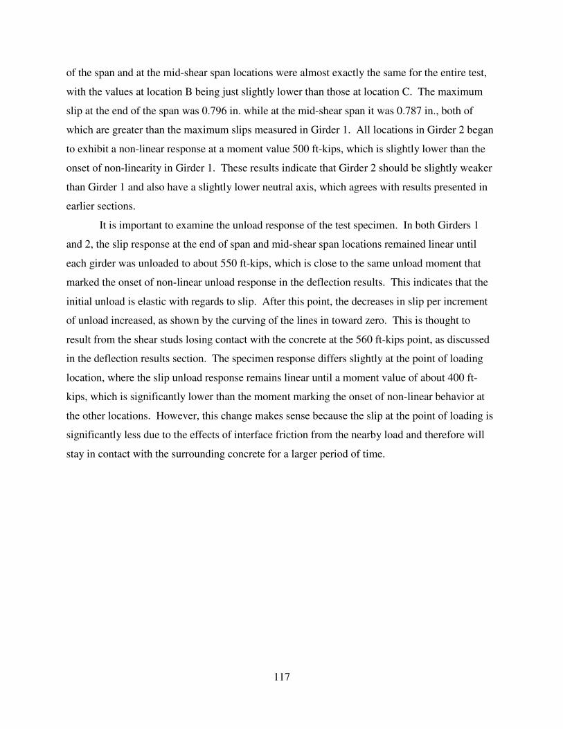
117

of the span and at the mid-shear span locations were almost exactly the same for the entire test,

with the values at location B being just slightly lower than those at location C. The maximum

slip at the end of the span was 0.796 in. while at the mid-shear span it was 0.787 in., both of

which are greater than the maximum slips measured in Girder 1. All locations in Girder 2 began

to exhibit a non-linear response at a moment value 500 ft-kips, which is slightly lower than the

onset of non-linearity in Girder 1. These results indicate that Girder 2 should be slightly weaker

than Girder 1 and also have a slightly lower neutral axis, which agrees with results presented in

earlier sections.

It is important to examine the unload response of the test specimen. In both Girders 1

and 2, the slip response at the end of span and mid-shear span locations remained linear until

each girder was unloaded to about 550 ft-kips, which is close to the same unload moment that

marked the onset of non-linear unload response in the deflection results. This indicates that the

initial unload is elastic with regards to slip. After this point, the decreases in slip per increment

of unload increased, as shown by the curving of the lines in toward zero. This is thought to

result from the shear studs losing contact with the concrete at the 560 ft-kips point, as discussed

in the deflection results section. The specimen response differs slightly at the point of loading

location, where the slip unload response remains linear until a moment value of about 400 ft-

kips, which is significantly lower than the moment marking the onset of non-linear behavior at

the other locations. However, this change makes sense because the slip at the point of loading is

significantly less due to the effects of interface friction from the nearby load and therefore will

stay in contact with the surrounding concrete for a larger period of time.

118

Slip (in.)

0.0 0.1 0.2 0.3 0.4 0.5 0.6 0.7 0.8 0.9

Mm

(ft

-kip

s)

0

100

200

300

400

500

600

700

800

900

1000





Slip (in.)

0.0 0.1 0.2 0.3 0.4 0.5 0.6 0.7 0.8 0.9

Mm

(ft

-kip

s)

0

100

200

300

400

500

600

700

800

900

1000





119

6.4 Static Testing Design Implications

The results of both static tests to failure (Tests 2 and 3) show that the measured moment

strengths for both the one stud per rib and two studs per rib layouts were below the calculated

values, with the results of Static Test 3 being slightly closer to the calculated values than Static

Test 2. The predicted values were based on individual shear stud strengths calculated using the

design equation (Eq. 2.26) given in the American Institute of Steel Construction’s Steel Design

Manual (2005). It is believed that this occurred because the shear studs did not reach their full

calculated capacity because the steel deck form ruptured at a lower load than anticipated, leading

to blowouts through the rib web that caused a reduced resistance to slip at the steel-concrete

interface. This failure mode was observed in both Tests 2 and 3. This also supports the design

assumption of weak side stud placement. To adjust for this, the reduction factors to the full shear

stud strength (AsFu) in the AISC specification (2005) provisions used to account for the number

of studs in a rib (Rg) and for strong or weak side placement (Rp) must be reduced to allow for this

lower shear stud strength. Because the measured values in Test 3 were closer to the calculated,

Test 3 must be examined first to determine an appropriate value for Rp because Rg appears to

have less of an effect on this layout and therefore will be kept equal to 1.0. To get the calculated

value of the plastic moment capacity to match the measured value in Test 3, the Rp factor has to

be reduced from 0.6 to 0.47. This new value of Rp is supported by the findings of Rambo-

Roddenberry (2002), where testing showed that the appropriate value for Rp is 0.48. The new Rg

factor is found by applying the Rp of 0.47 to the calculated value of the plastic moment for Test 2

and then reducing Rg down from 0.85 (for two studs per rib) until the calculated value equaled

the measured value. This occurs at an Rg value of 0.7, which is less than the design value

reported in Roddenberry (2002) of 0.85.

The linear elastic response of all three static tests conducted show that the calculated

deflections in the elastic range using the AISC commentary provisions (2005) for the effective

moment of inertia (Ieff) equation, both unreduced and with the recommended 0.75 reduction

factor applied, are greater than the measured values in testing. Therefore, the deflection values

calculated using the unreduced Ieff are a more accurate predictor of the test specimen response

while still remaining slightly on the conservative side. Also, it is important to note that the

calculated values were a little bit closer to the measured values in the one stud per rib layout, a

fact observed in the fatigue testing as well, although not enough to make a significant difference.

120

6.5 Summary of Laboratory Static Testing

In order to determine the ultimate moment strength of a bridge constructed using

continuous permanent metal deck forms, independent static testing was conducted on each half

of the test specimen. Each half of the specimen was loaded until it stopped taking load,

indicating that the moment capacity of that half had been reached. The goal was to compare the

measured moment capacities of the two different levels of partial composite action to the values

calculated using current AISC specification (2005) provisions to determine if they were

applicable to this construction method or if modifications had to be made to facilitate this

system. Three static tests were run on the test specimen. Static Test 1 was conducted on the

near side; however it was only loaded in the elastic range of the near side to gather data on the

elastic response. Static Test 2 was conducted on the far side of the bridge and was loaded until a

point after the plastic moment capacity had been achieved. Static Test 3 was conducted back at

the near side and was loaded until past the point where the plastic moment had been attained.

The results from Test 1 verified that Test 2 had not significantly affected the results of Test 3.

Measurements of load, deflection, strain, and slip were taken for both girders in each of

the tests conducted. The load and deflection data was used to determine the plastic moment

capacity of each girder while the strain and slip data was used as a method of describing the

moment-deflection results observed. A summary of the measured and calculated moment

capacities for the two pertinent static tests is provided in Table 6.1. As can be seen, the

measured values of the plastic moment capacities for Tests 2 and 3 were below the values

calculated using AISC (2005) provisions. To get the calculated plastic moment capacity values

to match the measured, modifications to the full shear stud strength reduction factors are

necessary. For one stud per rib, Rg must remain at 1.0 while Rp must be changed from 0.6 to

0.47 and for two studs per rib, Rg changed from 0.85 to 0.7 and Rp will change from 0.6 to 0.47

as noted.

Table 6.1: Summary of laboratory static testing

Measured (ft-kips) Calculated (ft-kips) % Difference

Static Test 2 - Girder 1 984 1150 -14.4%




Plastic Moment CapacityTest

121

Chapter 7: Conclusions and Recommendations

7.1 Conclusions

The continuous permanent metal deck form system provides a quick and efficient method

of constructing short-span simply supported composite steel girder bridges. However, because

shear studs have to be welded to the girder through the steel deck at rib locations, the number of

shear stud locations is limited to the number of ribs in the shear span while the spacing of the

shear studs is restricted to the rib spacing of the steel deck. This results in a condition where the

fatigue resistance provisions in the AASHTO LRFD Bridge Design Specifications (2007) cannot

be satisfied because the rib spacing of the steel deck, and therefore the shear stud spacing, is

almost always larger than the maximum stud spacing calculated from the AASHTO shear stud

fatigue resistance equation. Also, because the number of shear studs that can be used is limited

by the number of ribs, it is possible that a partial composite system will result if there are not

enough studs to create a fully composite system when the maximum numbers of studs per rib are

used. Currently, the AASHTO LRFD (2007) does not allow for the partial composite design of

bridges.

The purpose of this research was to investigate the fatigue resistance and static strength

of a full-scale bridge test specimen, designed as a typical two interior girder section, constructed

using the continuous permanent metal deck form system at two different levels of composite

action that utilized a one and two studs per rib layout. Fatigue testing was conducted to

determine the fatigue resistance of the specimen at both levels of interaction and then evaluated.

This was followed by static tests to failure to determine the plastic moment capacity at both

levels of interaction. Results of the testing were compared to existing design models and

modifications specific to this construction method are made.

7.1.1 Lateral Bracing by Steel Deck during Construction

Part of this research involved the investigation of whether the steel deck can be treated as

a shear diaphragm that provides adequate lateral restraint to the girder compression flange during

the placement of the concrete deck using the continuous permanent metal deck form system.

Current AASHTO LRFD (2007) provisions do not allow the steel deck to be treated as

continuous bracing for the steel girders. The goal was to determine if the steel deck is sufficient

122

to act as full compression flange bracing, during bridge construction, without the use of

intermediate diaphragms or cross frames, when shear studs are welded through the steel deck

into the girders. Therefore, the test specimen was constructed without intermediate diaphragms

or cross frames.

Calculations performed indicated that the steel deck used in the test specimen had

adequate strength and stiffness to provide full bracing during the deck placement. These results

were verified when the concrete deck was poured on the test specimen. The bottom flanges of

girders 1 and 2 only moved 0.263 in. and 0.262 in., respectively, outward from the longitudinal

centerline of the specimen, which represents about 0.31% of the girder spacing (7 ft). No other

significant changes were observed. It is important to point out that these results are applicable

only to the test setup used in this research and do not indicate that the steel deck can adequately

brace the steel girders in all applications.

7.1.2 Laboratory Fatigue Testing

Two fatigue tests were conducted as part of this research. The load range for each test

was calculated as the stress range on each shear stud required to cause failure at 1 million cycles

based on the AAHSTO LRFD (2007) fatigue design equation using the section properties of the

test specimen. The goal of the fatigue testing was determine if this design equation is overly

conservative for the continuous permanent metal deck form construction method with one and

two studs per rib. Measurements of vertical deflection, slip, and strain were taken at set

increments during each test to track the loss of stiffness in the specimen during each test.

Fatigue Test 1 was conducted at the near side quarter point of the test specimen with the

purpose of fatiguing the shear studs between the point of loading and near side end of span

where there was a one stud-per-rib design. A cyclic load with a range of 50 kips was distributed

to load points above each girder through a spreader beam for a total of 1,200,000 cycles, with no

failures occurring during the test. The vertical deflection at the point of loading in Girder 1

increased from -0.115 in. at the start of the test to -0.120 in. at one million cycles which

represents a 4.58% increase in deflection at the design number of cycles. Similarly, the vertical

deflection at the point of loading in Girder 2 increased from -0.115 in. at the start of the test to

-0.121 in. at one million cycles, which represents a 5.41% increase in deflection at the design

number of cycles.

123

Fatigue Test 2 was conducted at the far side quarter point of the test specimen with the

purpose of fatiguing the shear studs between the point of loading and far side end of span where

there was a two studs-per-rib design. A cyclic load with a range of 95 kips was distributed to

load points above each girder through a spreader beam for a total of 1,200,000 cycles, with no

failures occurring during the test. The vertical deflection at the point of loading in Girder 1

increased from -0.211 in. at the start of the test to -0.225 in. at one million cycles which

represents a 6.68% increase in deflection at the design number of cycles. Similarly, the vertical

deflection at the point of loading in Girder 2 increased from -0.217 in. at the start of the test to

-0.237 in. at one million cycles, which represents a 9.41% increase in deflection at the design

number of cycles. For this test, however, the majority of the increase in deflection occurred

during settling period in the first 100,000 cycles of testing, accounting for 87.9% and 79.4% of

the total increases in deflection at one million cycles for Girders 1 and 2, respectively. Settling

was observed in the first 50,000 cycles of Fatigue Test 1, it represented a smaller amount of the

increase in deflection.

The slip results at the steel-concrete interface for both fatigue tests displayed the same

pattern. The values for the slip grew at an increasing rate as both tests went on and showed no

signs of leveling off. Therefore, it can be assumed that slips will continue to grow, leading to a

loss of composite action in the system which will result in increased deflections as cycling

continues. However, there does not appear to be direct correlation between the increase in slip

and the increase in deflection, so even though slip continues to increase, deflection may continue

to increase in the same linear fashion. There is no indication that a failure was imminent in

either fatigue test or that any shear studs received significant damage as result of the cycling.

7.1.3 Laboratory Static Testing

Three static tests were conducted as part of this research. The first test was loaded only

in the linear-elastic region of the specimen and was used to validate the results of the third test.

The second and third static tests consisted of loading until a point after the plastic moment

capacity of the specimen had been reached. The values used to calculate the plastic moment

capacity of the shear spans for each test were based on the individual shear stud static strength as

calculated in the AISC Specification for Structural Steel Buildings (2005), as opposed to values

calculated using the AASHTO LRFD (2007) specifications. The AISC design model was used

124

because it takes into account the reduction of strength of a shear stud when placed in profiled

steel deck, whereas AASHTO does not.

Static Test 2 was conducted at the quarter point in the far half of the test specimen where

there was a two studs-per-rib layout. The calculated plastic moment capacity of this test location

was 1150 ft-kips. The maximum moment achieved in Girder 1 in this test was 984 ft-kips, which

is 14.4% lower than predicted. The maximum moment achieved in Girder 2 was 989 ft-kips,

which is 13.9% lower than predicted. Static Test 3 was conducted at the far half quarter point of

the specimen where there is a one stud-per-rib layout. The calculated plastic moment capacity of

this test location was 960 ft-kips. The maximum moment achieved in Girder 1 in this test was

890 ft-kips, which is 7.3% lower than predicted. The maximum moment achieved in Girder 2

was 879 ft-kips, which is 8.4% lower than predicted. The same shear stud failure mode was

observed in both tests, where the shear stud ruptured the steel deck due to excessive slip which

caused a blowout through the rib web.

The measured results of both tests to failure were lower than predicted, which is believed

to be the result of the individual shear studs not reaching their calculated capacity. To make the

calculated plastic moment values equal the measured values for both tests, the Rp modification

factor must be reduced from 0.6 to 0.47 for weak side placement and the Rg factor has to be

reduced from 0.85 to 0.7 for two studs-per-rib while staying equal to 1.0 for the one stud-per-rib

layout. Additionally, it was shown that the unreduced effective moment of inertia value as based

on AISC commentary provisions (2005) produces a more accurate prediction for the elastic

deflections in both tests.

7.2 Summary

The behavior of a full scale bridge specimen, designed as a typical two interior section of

a fictitious bridge and constructed using the continuous permanent metal deck form system,

under both fatigue and static loading conditions was considered for two different numbers of

shear studs in the span. An evaluation of the supplemental calculations and the laboratory testing

lead to the following conclusions:

• The steel deck formwork was sufficient in this case to act as full compression flange

lateral bracing for the top flange of the steel girders during the placement of the concrete

deck when the shear studs are welded through the steel deck into the girder.

125

− This removes the necessity to include intermediate diaphragms or cross-frames in

the span, which makes construction faster and more economical.

− These results do not imply that steel deck will be sufficient lateral bracing during

bridge construction in all cases. Bracing requirements will still need to be evaluated

on a case-by-case basis.

• Both the one and two studs-per-rib layouts lost very little stiffness over the course of the

load cycles applied with no failures occurring or appearing to be imminent in either

layout, which tells us that the AASHTO LRFD (2007) equation for shear stud fatigue

resistance is conservative when applied to this construction method.

− The one stud-per-rib layout lost less relative stiffness than the two studs-per-rib

layout during cycling; however, when the effects of specimen settling are taken into

account, the two studs-per-rib layout lost less stiffness than the one stud.

− Curves fit to the deflection data for both tests extrapolated to five million cycles

show that the deflections at that point are still well below the deflections expected

with no composite action between the girder and the deck

• The measured plastic moment capacities of both shear stud layouts were below their

respective calculated values due to the inability of the individual shear studs to develop

their full predicated capacities calculated using AISC specification (2005) design models

due to premature rupture of the steel deck leading to blowouts of the shear studs through

the rib webs.

− To get the calculated values to equal the measured values, for a one stud-per-rib

layout the Rg factor must stay equal to 1.0 while the Rp factor gets reduced from 0.6

to 0.47 while for the two studs-per-rib layout the Rg factor must get reduced from

0.85 to 0.7 and the Rp must again get reduced from 0.6 to 0.47.

• The full value of the AISC commentary (2005) equation for the effective moment of

inertia of a partial composite beam provides a more accurate prediction of the elastic

deflections of the test specimen than the 75% value recommended in the commentary.

− The predictions for elastic deflection using the full effective moment of inertia is

closer to the measured values, however the reduced value provides a more

conservative estimate.

126

7.3 Recommendations for Future Research

Based on the results of the fatigue and static tests conducted on the test specimen, it

appears that the continuous permanent metal deck form bridge construction method is a viable

alternative to current methods of bridge construction. However, before this system can be

implemented in real world environments, several aspects of the system require further research,

which are listed as follows:

• Research investigating just the shear diaphragm properties of the steel deck when it is

used as lateral compression flange bracing for the steel girders should be conducted. The

effects of different bridge span lengths, deeper girders, different girder spacing, and

strength of the steel deck connection to the girders when welded studs are used should be

studied so that provisions specific to this construction method can be created.

• Push out tests utilizing 7/8” shear studs welded through profiled steel deck in both the

weak and strong positions with one and two studs-per-rib layouts should be conducted to

determine the response of the system at failure to establish if modifications to existing

AISC specification (2005) provisions are necessary to accurately predict the failure

response.

• Longer life fatigue tests should be conducted to investigate whether the behavior observed

in this study will continue for the life of the specimen or if stabilization may occur at some

point in the fatigue life.

• Testing should be expanded beyond the short span, simply supported conditions with

rolled shapes studied in this research. Specimens constructed with built-up girders in a

continuous span system should be investigated to determine the response of the

continuous PMDF system with the additional fatigue considerations created if built-up

sections are used as well as the effects of moment reversal.

• Profiled steel deck of different height, shape, and gage that has been provided by

Wheeling Corrugating should be investigated to determine the effects of these variables on

strength

127

References:

American Association of State Highway and Transportation Officials (AASHTO). (2007).

AASHTO LRFD bridge design specifications, American Association of State Highway and

Transportation Officials, Washington, D.C.

American Institute of Steel Construction, Inc. (AISC). (2005). Commentary on the Specification

for Structural Steel Buildings, Chicago.

American Institute of Steel Construction, Inc. (AISC). (2005). Specification for Structural Steel

Buildings, 13th

ed. Chicago.

Barker, R.M., and Puckett, J.A. (2007). “Design of Highway Bridges, An LRFD Approach.” 2nd

ed., John Wiley and Sons, Inc., Hoboken, NJ.

Easterling, W.S, Gibbings, D.R., and Murray, T.M. (1993). “Strength of Shear Studs in Steel

Deck on Composite Beams and Joists.” Engineering Journal, 30(2), 44-55.

Egilmez, O.O., Helwig, T.A., Jetann, C.A., and Lowery, R. (2007). “Stiffness and Strength of

Metal Bridge Deck Forms.” Journal of Bridge Engineering, 12(4), 429-437.

Federal Highway Administration (FHWA). (2006). 2006 Status of the Nation's Highways,

Bridges, and Transit: Conditions and Performance, FHWA, Washington D.C.

Grant Jr., J.A., Fisher, J.W., and Slutter, R.G. (1977). “Composite Beams with Formed Steel

Deck.” Engineering Journal, 14(1), First Quarter, 24-43.

Helwig, T.A., and Frank, K.H. (1999). “Stiffness Requirements for Diaphragm Bracing of

Beams.” Journal of Structural Engineering, 125(11), 1249-1256.

Helwig, T.A., Frank, K.H., and Yura, J.A. (1997). “Lateral-Torsional Buckling of Singly

Symmetric I-Beams.” Journal of Structural Engineering, 123(9), 1172-1179.

Helwig, T.A., and Yura, J.A. (2008a). “Shear Diaphragm Bracing of Beams. I: Stiffness and

Strength Behavior.” Journal of Structural Engineering, 134(3), 348-356.

Helwig, T.A., and Yura, J.A. (2008b). “Shear Diaphragm Bracing of Beams. II: Design

Requirements.” Journal of Structural Engineering, 134(3), 357-363.

Johnson, R.P. (1981). “Loss of Interaction in Short-Span Composite Beams and Plates.” Journal

of Constructional Steel Research, 1(2), 11-16.

Johnson, R.P. (1995). “Composite Structures of Steel and Concrete, Volume 1: Beams, Slabs,

Columns, and Frames for Buildings.” Blackwell Scientific Publications, London.

Johnson, R.P., and May, I.M. (1975). “Partial Interaction Design of Composite Beams.” The

Structural Engineer, 53(8), 305-311.

Kwon, G., Hungerford, B., Kayir, J., Schaap, B., Ju, Y.K., Klingner, R.E. and Engelhardt, M.D.

(2007). “Strengthening of Existing Non-Composite Steel Girder Bridges Using Post-

Installed Shear Connectors.” Texas Univ. at Austin Center for Transportation Research.

Luttrell, L.D. (2004). Steel Deck Institute Design Manual, 3rd

Edition, Canton, Ohio.

McGarraugh, J.B., and Baldwin, J.W. (1971). “Lightweight Concrete-on-Steel Composite

Beams.” AISC Eng. J., 8(3), 90-98.

128

Oehlers, D.J., and Bradford, M.A. (1995). “Composite Steel and Concrete Structural Members”.

Elsevier Science, Inc., New York, New York.

Oehlers, D.J. and Foley, L. (1985). “The Fatigue Strength of Stud Shear Connections in

Composite Beams.” Proc. Instn. Civ. Engrs., 79(2), 349-364.

Oehlers, D.J., Seracino, R., and Yeo, M.F. (2000). “Effect of Friction on Shear Connection in

Composite Bridge Beams.” Journal of Bridge Engineering, 5(2), 91-98.

Ollgaard, J.G., Slutter, R.G., and Fisher, J.W. (1971). “Shear Strength of Stud Connectors in

Lightweight and Normal Weight Concrete.” AISC Engineering Journal, 8(2),55-64.

Rambo-Roddenberry, M.D. (2002). “Behavior and Strength of Welded Stud Shear Connectors.”

PhD Dissertation, Virginia Polytechnic Institute and State University, Blacksburg, VA.

Salmon, C.G, and Johnson, J.E. (1996). Steel Structures: Design and Behavior.” 4th

Edition,

Prentice Hall, Upper Saddle River, NJ.

Slutter, R.G., and Fisher, J.W. (1967). “Fatigue Strength of Shear Connectors.” Highway

Research Record, 147, 65-88.

Winter, G. (1960), “Lateral Bracing of Columns and Beams.” ASCE Transactions, Vol. 125, pp.

809-825.

Wu, Y.F., Oehlers, D.J., and Griffith, M.C. (2002). “Partial-Interaction Analysis of Composite

Beam/Column Members.” Mechanics of Structures and Machines, 30(3), 309-332.

Yura, J.A. (1995). “Bracing for Stability-State-of-the-Art.” Proceedings, Structures Congress

XIII, ASCE, New York, 88-103.

Yura, J.A. (2001). “Fundamentals of Beam Bracing.” Engineering Journal, 38(1), 11-26.

Yura, J. A., Phillips, B., Raju, S., and Webb, S. (1992), “Bracing of Steel Beams in Bridges,”

Report No. 1239-4F, Center for Transportation Research, University of Texas at Austin,

October, 80 p.

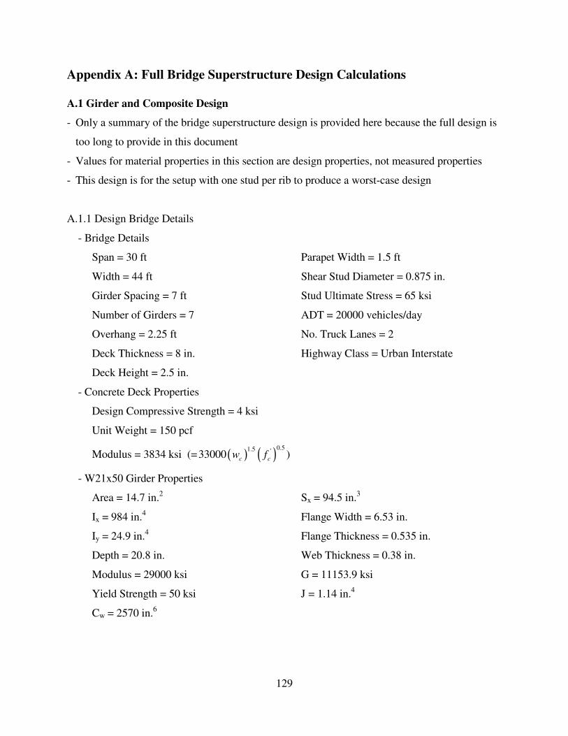
129

Appendix A: Full Bridge Superstructure Design Calculations

A.1 Girder and Composite Design

- Only a summary of the bridge superstructure design is provided here because the full design is

too long to provide in this document

- Values for material properties in this section are design properties, not measured properties

- This design is for the setup with one stud per rib to produce a worst-case design

A.1.1 Design Bridge Details

- Bridge Details

Span = 30 ft Parapet Width = 1.5 ft

Width = 44 ft Shear Stud Diameter = 0.875 in.

Girder Spacing = 7 ft Stud Ultimate Stress = 65 ksi

Number of Girders = 7 ADT = 20000 vehicles/day

Overhang = 2.25 ft No. Truck Lanes = 2

Deck Thickness = 8 in. Highway Class = Urban Interstate

Deck Height = 2.5 in.

- Concrete Deck Properties

Design Compressive Strength = 4 ksi

Unit Weight = 150 pcf

Modulus = 3834 ksi (= ( ) ( )0.51.5 '33000

c cw f )

- W21x50 Girder Properties

Area = 14.7 in.2 Sx = 94.5 in.

3

Ix = 984 in.4 Flange Width = 6.53 in.

Iy = 24.9 in.4 Flange Thickness = 0.535 in.

Depth = 20.8 in. Web Thickness = 0.38 in.

Modulus = 29000 ksi G = 11153.9 ksi

Yield Strength = 50 ksi J = 1.14 in.4

Cw = 2570 in.6

130

A.1.2 Interior Girder Design Moments and Shears

- W21x50 Girder Properties

Moment Distribution Factor = 0.595 (based on two or more lanes loaded)

Fatigue Moment Distribution Factor = 0.391

Shear Distribution Factor = 0.743

- Dead Loads on Girders

Deck = 0.853 kip/ft (0.853 kip/ft per girder)

Girder Self-Wt = 50 lb/ft (0.05 kip/ft per girder)

Stay-in-Place = 20 psf (0.14 kip/ft per girder)

Construction Excesses = 20 psf (0.14 kip/ft per girder)

- Dead Loads on the Composite Section

Wearing Surface = 15 psf (0.105 kip/ft per girder)

Barrier = 0.3 kip/ft (0.043 kip/ft per girder)

- Factored Moment and Shears

Taken at centerline of bridge

Table A.1: Interior girder factored moments and shears

Strength I Service I Service II Fatigue

133.10 4.82 11.81 301.28 717.36 451.01 541.40 68.45

Strength I Service I Service II

17.75 0.64 1.58 56.17 123.65 76.14 92.99

DL+WS+

1.30LLDL+WS+LL

1.25DL+1.50

WS+1.75LL

Live Load

(kips)

Wearing

(kips)

Barrier

(kips)

Dead Load

(kips)

Interior Shear Envelope

Interior Moment Envelope

Dead Load Barrier Wearing Live Load 1.25DL+1.50

WS+1.75LLDL+WS+ LL

DL+WS+

1.30LL0.75Fatigue

A.1.3 Interior Girder Composite Section Properties

- Effective Deck Flange Width

Effective Flange Width = 7 ft (Girder spacing)

- Short and Long Term Section Properties (for one stud per rib)

131

Table A.2: Composite Section Properties

Property Short Term Long Term

Ix,trans (in.4) 4476 3432

Sbot girder (in.3) 187.6 165.2

Stop girder (in.3) 1070.6 3693.6

A.1.4 Constructability Check

- Flexure � based on Continuous Bracing Condition

Construction Loading = 166.4 kip-ft

fbu = 21.1 ksi (largest stress in the compression flange under construction loading)

Resistance = f h yfR Fφ = 50 ksi ∴OK

- Shear

Construction Loading = 22.2 kips

/w

D t = 51.9 ∴C = 1.0

v nVφ = 217.4 kips ∴OK

A.1.5 Service Limit State

- Stress Limits

Bottom Flange = 47.5 ksi

Top Flange = 47.5 ksi

- Service Limit Stress Check

Table A.3: Service limit state stress check

Load Moment Seff,bot Stress

Dead 1597.22 94.50 16.90

Barrier 57.86 165.22 0.35

Wearing Surface 141.75 165.22 0.86

Live 4699.94 187.63 25.05

∑ 43.16 ksi

Bottom Flange

Bottom Flange Limit = 47.5 ksi > Total Service Stress = 43.16 ksi ∴OK

132

A.1.6 Fatigue Limit State

- Stress Range

ADTTSL = 2550 Trucks/day

N = number of cycles in structure life = 164250000 cycles

A = 4400000000 ksi3

(A/N)1/3

= 2.992 ksi

(∆f) = 4.377 ksi

- Fatigue Resistance

Based on Fatigue Category A

(∆F)TH = 24 ksi

0.5(∆F)TH = 12 ksi > (∆f) = 4.377 ksi ∴OK

A.1.7 Shear Stud Required Fatigue Pitch

- Background Calculations

N = 164250000 cycles

Zr = 2.105 kips

Ix = 4476 in.4

Q = 213.2 in.3

Distribution Factor = 0.568

Load Factor = 0.75

Number of Studs/Row = 1

- Required Shear Stud Spacing

Table A.4: Required shear stud fatigue spacing – 1 stud per rib

Location (ft) Max. Pos. Shear Factored Pos. Max. Neg. Shear Factored Neg. Range Pitch (in.)

0 36.27 23.67 4.27 0 17.76 2.49

3 32.27 21.06 0.27 0 15.80 2.80

6 28.27 18.45 -3.73 -2.44 15.67 2.82

9 24.27 15.84 -7.73 -5.05 15.67 2.82

12 20.27 13.23 -11.73 -7.66 15.67 2.82

15 16.27 10.62 -15.73 -10.27 15.67 2.82

A.1.8 Strength Limit State

- Is section compact

D/tw = 51.9 ∴OK

133

Fy = 50 ksi ∴OK

(2Dcp)/tw = 0 ∴OK

Section is compact

- Shear Check

Vu = 123.7 kips

v nVφ = 217.4 kips ∴OK

- Ductility Check

0.42Dt = 12.15 in. > Dp = 2.57 in.

- Bearing Check

Based on 7 in. bearing length

Web Buckling

uR = 123.65 kips

nbRφ = 182.40 kips ∴OK

Web Crippling

uR = 123.65 kips

nwRφ = 111.32 kips ∴NOT OK � Bearing stiffeners required

- Bearing Stiffener Design

Use a plate 3 in. wide by 0.375 in. thick

(KL)/r = 11.44

λ = 0.0165

uR = 123.65 kips

ncPφ = 156.04 kips

- Flexural Capacity – Partial Composite (1 stud per rib, weak side placement)

nQ = 23.45 kips/stud

N = 23 studs to the point f maximum moment

∑ nQ = 539.9 kips

uM = 717.4 kips

nMφ = 957.7 ft-kips ∴OK

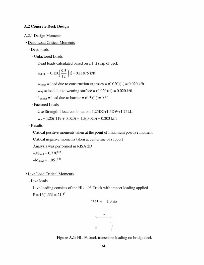
134

A.2 Concrete Deck Design

A.2.1 Design Moments

• Dead Load Critical Moments

- Dead loads

▫ Unfactored Loads

Dead loads calculated based on a 1 ft strip of deck

wdeck = ( ) =

1

12

5.9150.0 0.11875 k/ft

wconst = load due to construction excesses = (0.020)(1) = 0.020 k/ft

wws = load due to wearing surface = (0.020)(1) = 0.020 k/ft

Lbarrier = load due to barrier = (0.3)(1) = 0.3k

▫ Factored Loads

Use Strength I load combination: 1.25DC+1.5DW+1.75LL

wu = 1.25(.119 + 0.020) + 1.5(0.020) = 0.203 k/ft

- Results

Critical positive moments taken at the point of maximum positive moment

Critical negative moments taken at centerline of support

Analysis was performed in RISA 2D

+Mdead = 0.770k-ft

–Mdead = 1.051k-ft

• Live Load Critical Moments

- Live loads

Live loading consists of the HL – 93 Truck with impact loading applied

P = 16(1.33) = 21.3k

6'

21.3 kips 21.3 kips

Figure A.1: HL-93 truck transverse loading on bridge deck

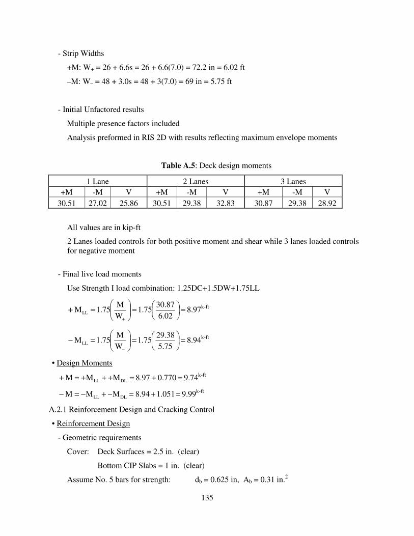
135

- Strip Widths

+M: W+ = 26 + 6.6s = 26 + 6.6(7.0) = 72.2 in = 6.02 ft

–M: W– = 48 + 3.0s = 48 + 3(7.0) = 69 in = 5.75 ft

- Initial Unfactored results

Multiple presence factors included

Analysis preformed in RIS 2D with results reflecting maximum envelope moments

Table A.5: Deck design moments

1 Lane 2 Lanes 3 Lanes

+M -M V +M -M V +M -M V

30.51 27.02 25.86 30.51 29.38 32.83 30.87 29.38 28.92

All values are in kip-ft

2 Lanes loaded controls for both positive moment and shear while 3 lanes loaded controls

for negative moment

- Final live load moments

Use Strength I load combination: 1.25DC+1.5DW+1.75LL

=

=

=+

+ 6.02

30.871.75

W

M1.75MLL 8.97

k-ft

=

=

=−

− 5.75

29.381.75

W

M1.75MLL 8.94

k-ft

• Design Moments

=+=+++=+ 0.77097.8MMM DLLL 9.74k-ft

=+=−+−=− 051.194.8MMM DLLL 9.99k-ft

A.2.1 Reinforcement Design and Cracking Control

• Reinforcement Design

- Geometric requirements

Cover: Deck Surfaces = 2.5 in. (clear)

Bottom CIP Slabs = 1 in. (clear)

Assume No. 5 bars for strength: db = 0.625 in, Ab = 0.31 in.2

136

dpos = =−−−2

625.00.15.08 6.19 in.

dneg = =−−2

625.05.28 5.19 in.

Smax = 1.5t = 1.5(8) = 12 in.

- Positive reinforcement

▫ Determine bar size and spacing

+M = 9.74k-ft

Snc = section modulus of deck = ( )( )=

= 33 812

6

1bh

6

1128 in.

3

fr = Concrete Modulus of Rupture = == 437.0f37.0 '

c 0.74 ksi

Mcr = Sncfr = (128)(0.74) = 94.72k-in

= 7.89k-ft

Min. Mu = 1.2Mcr = 1.2(7.89) = 9.74k-ft

min 1.33Mu = 1.33(9.74)

Trial As = ( )

==6.194

9.74

4d

Mu 0.393 in.2

Try No. 5 bars at 9 in (As = 0.41 in.2/ft)

▫ Check ductility and strength

( )( )( )( )( )

===1240.85

600.41

b0.85f

fAa

'

c

ys0.603 in.

0.35d = 0.35(6.19) = 2.17 in > 0.603 ∴OK

( )( ) =

−=

−=

2

0.6036.19600.410.9

2

adfφAφM ysn 10.86

k-ft > Mu = 9.74

k-ft

∴Use No. 5 bars at 9 in spacing, As = 0.41 in.2

- Negative reinforcement


–M = 9.99k-ft

Min. Mu = 1.2Mcr = 1.2(7.89) = 9.74k-ft

min 1.33Mu = 1.33(9.99)

137

Trial As = ( )

==5.194

9.74

4d

Mu 0.469 in.2

Try No. 5 bars at 8 in. (As = 0.46 in.2/ft)

▫ Check ductility and strength

( )( )( )( )( )

===1240.85

600.46

b0.85f

fAa

'

c

ys0.676 in.

0.35d = 0.35(5.19) = 1.82 in. > 0.603 in. ∴OK

( )( ) =

−=

−=

2

0.6765.19600.460.9

2

adfφAφM ysn 10.04

k-ft > Mu = 9.99

k-ft


- Secondary reinforcement


Placed at the bottom of the slab (inside primary reinforcement)

7.0Se =

ft

===7.0

220

S

220ρ

e

s 83% > 67%, ∴ =sρ 67%

As,sec = ρs(As,pos) = 0.67(0.41) = 0.27 in2/ft


- Temperature and shrinkage reinforcement

As,T+S ( )( )

==60

1280.11

f

A0.11

y

g0.18 in.

2/ft

Distribute reinforcement equally on both faces, As,T+S = 0.5(0.18) = 0.09 in.2/ft

∴Use No. 4 bars at 12 in spacing (Smax)

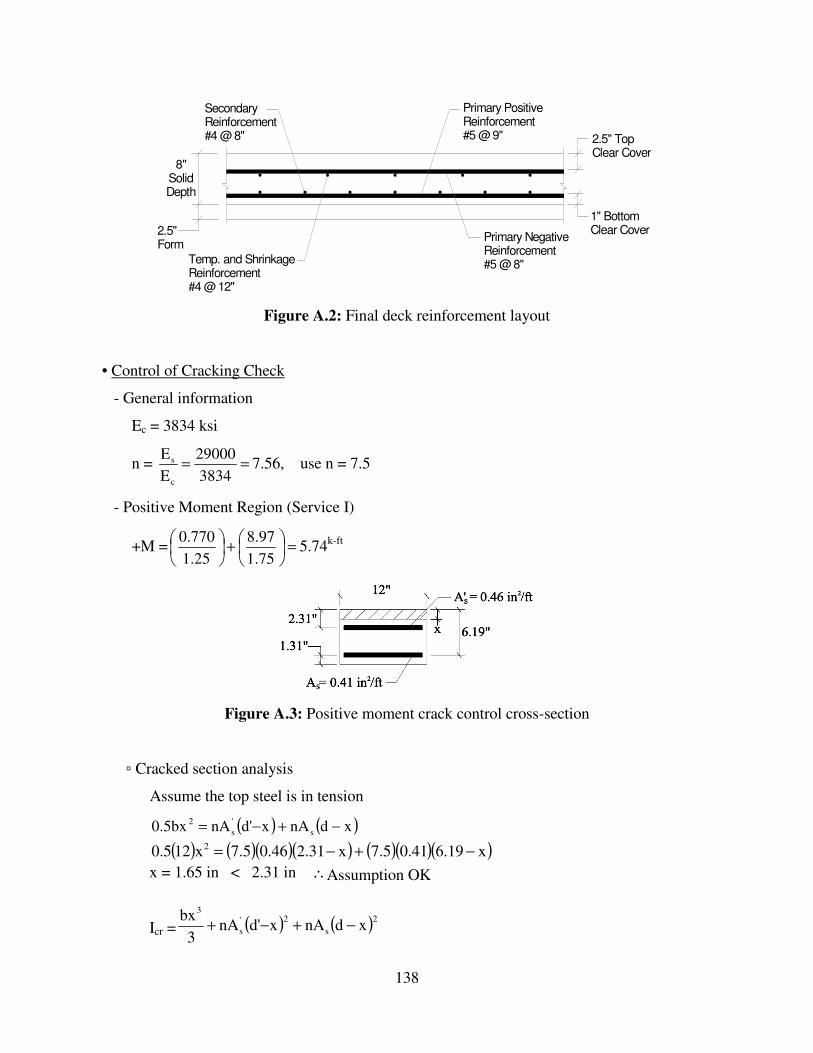
138

8"SolidDepth

SecondaryReinforcement#4 @ 8"

Primary PositiveReinforcement#5 @ 9"

Primary NegativeReinforcement#5 @ 8"Temp. and Shrinkage

Reinforcement#4 @ 12"

2.5" TopClear Cover

1" BottomClear Cover2.5"

Form

Figure A.2: Final deck reinforcement layout

• Control of Cracking Check

- General information

Ec = 3834 ksi

n = ==3834

29000

E

E

c

s 7.56, use n = 7.5

- Positive Moment Region (Service I)

+M = =

+

75.1

97.8

25.1

770.05.74

k-ft

Figure A.3: Positive moment crack control cross-section

▫ Cracked section analysis

Assume the top steel is in tension

( ) ( )xdnAxd'nA0.5bx s

'

s

2 −+−=

( ) ( )( )( ) ( )( )( )x6.190.417.5x2.310.467.5x120.5 2 −+−=

x = 1.65 in < 2.31 in ∴Assumption OK

Icr = ( ) ( )2

s

2'

s

3

xdnAxd'nA3

bx−+−+

139

Icr =( )( ) ( )( )( ) ( )( )( )22

3

65.119.641.05.765.131.246.05.73

65.112−+−+

Icr = 82.85 in.4/ft

▫ Calculate maximum spacing

( )( )( )( )=

−=

=

82.85

1.656.19125.747.5

I

Mynf

cr

s 28.31 ksi

γe = 0.75 (Class 2 Exposure)

dc = 1.31 in.

βs = ( ) ( )

=−

+=−

+1.3180.7

1.311

d80.7

d1

c

c 1.28

Smax = ( )( )

( )( )==

28.311.28

0.75700

fβ

700γ

ss

e 14.49 in > S = 9 in. ∴OK

Positive reinforcement provided is sufficient for control of cracking

- Negative Moment Region (Service I)

=

+

=−

1.75

8.94

1.25

1.051M 5.95

k-ft

Figure A.4: Negative moment crack control cross-section

▫ Cracked section analysis

Assume the bottom steel is in compression

( ) ( ) ( )xdnA'dxA1-n0.5bx s

'

s

2 −+−−=

( ) ( )( )( ) ( )( )( )x5.190.467.531.1x0.411-7.5x120.5 2 −+−−=

x = 1.44 in. > 1.31 in. ∴Assumption OK

140

Icr = ( ) ( )2

s

2'

s

3

xdnA'dxnA3

bx−+−+

Icr =( )( ) ( )( )( ) ( )( )( )22

3

44.119.646.05.731.144.141.015.73

44.112−+−−+

Icr = 89.83 in.4/ft

▫ Calculate maximum spacing

( )( )( )( )=

−=

=

89.83

1.445.19125.957.5

I

Mynf

cr

s 22.35 ksi

γe = 1.0 (Class 1 Exposure)

dc = 2.31 in.

βs = ( ) ( )

=−

+=−

+2.3180.7

2.311

d80.7

d1

c

c 1.58

Smax = ( )( )

( )( )==

22.351.58

1.0700

fβ

700γ

ss

e 19.82 in. > S = 10 in. ∴OK

Negative reinforcement provided is sufficient for control of cracking

• Shear Design

- Two way shear (punching shear)

▫ Determine tire patch area

W = ( ) =

=

+

5.2

1633.175.1

5.21001

PIMγ 14.90 in.

d = 6.69 in.

bo = 20 + 6.69 + 14.9 + 6.69 = 48.28 in.

▫ Determine shear capacity of slab

dv = T to C = 6.19 – 0.5(2.31) = 5.04 in. � dv = 5.04 in.

0.9de = 0.9(6.19) = 5.57 in.

min 0.72h = 0.72(8) = 5.76 in.

βc = ratio of long side to short side of tire patch =( )

( )=

+

+

69.69.14

69.6201.24

141

( )( ) =

+=

+= 04.528.484

1.24

126.0063.0dbf

β

0.1260.063V vo

'

c

c

c 80.1k

( )( ) === 5.0448.2840.126dbf0.126V vo

'

ccmax 61.3k ∴Vn = 61.3k

φVn = 0.9(61.3) = 55.17k

Vu = (1.75)(1.33)(16) = 37.24k < φVn = 55.17k ∴OK

- One way shear (beam shear)

▫ Determine tire patch area

( ) ( ) ( )( ) === 5.0412420.0316dbf20.0316V vv

'

cc 7.64k

( )( )( ) ==≤ 5.041240.25dbf25.0V vv

'

cc60.48

k

φVc = 0.9(7.64) = 6.88k

Loads taken at dv from flange tip

( ) =

= 1.75

6.30

22.369V trucku,

6.21k

=deadu,V 0.358k

Vu = 6.21 + 0.358 = 6.57k

< φVc = 6.88k ∴OK

A.3 Steel Deck Design

A.3.1 Design Moments

- Design loads

qs = weight of solid slab = ( ) =

12

8150 100 psf

qr = weight of concrete in flutes = ( ) =

12

1150 12.5 psf

qc = construction load = 50 psf

qf = weight of 20 gage form = 2.25 psf

wt = ( )( ) ( )( ) =+++=+++ ft125.2505.12100ft1fcrs qqqq 164.75 lb/ft

142

- Design Moments

▪ Moments calculated using RISA 2D

Design Span = 7 ft

Figure A.5: RISA 2D moment graphic output for steel deck

+Mmax = 436 lb-ft = 5232 in.-lb

−Mmax = −741 lb-ft = −8892 in.-lb

A.3.2 Stress Checks

- Allowable stress

fa = 36000 psi

- Resisting moment

Sp = section modulus of form = 0.457 in3

( )( ) === 457.036000par SfM 16452 in-lb

A.3.3 Deflection Checks

- Allowable deflection

( )===∆

800

127

800

Lall 0.467 in. < 0.5 in.

- Form Deflection

Ip = moment of inertia of form = 0.623 in.4

▪ Deflections calculated assuming simply supported to produce an upper bound

( )( )( ) ( )( )( )( )

===∆623.029000384

1728716475.05

384

544

maxEI

wL0.492 in.

▪ Deflections calculated assuming fixed ends to produce a lower bound

( )( ) ( )( )( )( )

===∆623.029000384

1728716475.0

384

44

maxEI

wL0.099 in.

▪ Actual deflection will lie closer to fixed end condition, therefore deflection check is OK

143

Appendix B: Fatigue Load Range Calculations

B.1 Background Information

B.1.1 AASHTO LRFD (2007) Design Equation

- Base equation

p = pitch of shear studs sr

r

V

nZ≤

n = number of shear connectors per group

Zr = fatigue resistance of an individual shear connector = 22

2

5.5dd

>α

Nlog28.45.34 −=α

d = shank diameter of shear connector

N = number of cycles in the design life

Vsr = horizontal fatigue shear range per unit length = ( ) ( )22

fatfat FV +

Vfat = longitudinal shear force per unit length = I

QV f

Q = first moment of inertia of transformed system

Vf = vertical shear force range under the fatigue load

I = second moment of inertia of transformed section

Ffat = radial fatigue shear range per unit length

B.1.1 Modified Equation for Testing

- Shear connector pitch (p) is set at the rib spacing (8 in.)

- Equation is solved for the required vertical shear range to cause failure at 1,000,000 million

cycles

p

nZV r

sr =

▪ Specimen is not curved or skewed 0=∴ fatF

( ) ( ) ( ) ( )I

QVVVFVV

f

fatfatfatfatsr ==+=+=2222

0

144

pQ

InZV r

f =∴

- Vertical shear in shear span

P

0.75P 0.25P

L

0.25L 0.75L

0.75P

0.25P

Girder Reactions

Girder Vertical Shear

Figure B.1: Girder reactions and vertical shear with quarter point loading

- Load required to reach a given vertical shear

PV f4

3= � fdreq VP

3

4' =∴

B.2 Fatigue Test 1

B.2.1 AASHTO LRFD Load Range

- Moment of Inertia

▪ Static strength of shear studs assuming weak side placement from AISC Steel Design

Manual (2005)

Qn = min(Qn1, Qn2)

=

==

2

2

2

875.0ππ rAsc 0.6013 in.

2

( ) ( )( ) === 44008.56013.05.05.0 '

1 ccscn EfAQ 48.03 kips

145

( )( )( )( ) === 656013.00.16.02 uscgpn FARRQ 23.45 kips

Qn2 controls =∴ nQ 23.45 kips

▪ Moment of inertia calculated using AISC Steel Design Manual (2005) equation for

effective moment of inertia with partial shear connection

( ) ( )( )( )( )

( ) =−+=−+=∑

9844.5162607.14

45.2312984str

f

n

seff IIC

QII 3344.14 in.

4

- Individual connector shear resistance (Zr)

( ) =−=−= 000,000,1log28.45.34log28.45.34 Nα 8.82

( )( ) ===22 875.082.8dZ r α 6.753 kips

( ) =

=

22875.0

2

5.5

2

5.5d 2.105 kips < Zr = 6.753 kips ∴OK

- First moment of inertia (Q)

▪ Value for distance to neutral axis (yb) taken from strain gauge test results

=

−=

−= 7.14

2

8.2035.22

2gb A

dyQ 175.67 in.3

- Vertical shear range required

( )( )( )( )( )

===67.1758

1.3344753.61',

pQ

InZV xr

dreqf 16.07 kips

- Quarter-point load required to achieve this vertical shear range

=

== 07.16

3

4

3

4',' dreqfdreq VP 21.4 kips

- Use a load range of 25 kips/girder

▪ Accounts for a conservative value for Ix calculated using the AISC equation

B.2.2 Load per Shear Connector

- Horizontal shear per unit length at interface

( )( )( )===

1.3344

67.17575.0252

x

f

I

QVq 0.985 kips/in.

146

- Force per shear connector

( )( )===

1

985.08

n

pqFcon 7.88 kips

B.3 Fatigue Test 2

B.3.1 AASHTO LRFD Load Range

- Moment of Inertia

▪ Static strength of shear studs with weak side placement from AISC Steel Design

Manual (2005)

Qn = min(Qn1, Qn2)

=

==

2

2

2

875.0ππ rAsc 0.6013 in.

2

( ) ( )( ) === 44008.56013.05.05.0 '

1 ccscn EfAQ 48.03 kips

( )( )( )( ) === 656013.085.06.02 uscgpn FARRQ 19.93 kips

Qn2 controls =∴ nQ 19.93 kips

▪ Moment of inertia calculated using AISC Steel Design Manual (2005) equation for

effective moment of inertia with partial shear connection

( ) ( )( )( )( )

( ) =−+=−+=∑

9844.5162607.14

93.1924984str

f

n

seff IIC

QII 4061.1 in.

4

- Individual connector shear resistance (Zr)

( ) =−=−= 000,000,1log28.45.34log28.45.34 Nα 8.82

( )( ) ===22 875.082.8dZ r α 6.753 kips

( ) =

=

22875.0

2

5.5

2

5.5d 2.105 kips < Zr = 6.753 kips ∴OK

- First moment of inertia (Q)

▪ Value for distance to neutral axis (yb) taken from strain gauge test results

=

−=

−= 7.14

2

8.2036.23

2gb A

dyQ 190.57 in.

3

147

- Vertical shear range required

( )( )( )( )( )

===57.1908

1.4061753.62',

pQ

InZV xr

dreqf 35.98 kips

- Quarter-point load required to achieve this vertical shear range

=

== 98.35

3

4

3

4',' dreqfdreq VP 47.9 kips

B.3.2 Load per Shear Connector

- Horizontal shear per unit length at interface

( )( )===

1.4061

57.1909.372

x

f

I

QVq 1.778 kips/in.

- Force per shear connector

( )( )===

2

778.18

n

pqFcon 7.112 kips

- Use a load range of 47.5 kips/girder

▪ this is at the very upper limit of the testing equipment at reasonable run rates

148

Appendix C: Material Property Results

C.1 Concrete Properties

C.1.1 Concrete Compressive Strength Results

- 4 in. by 8 in. cylinders used

- Two cylinders per truck at each of 7, 14, 21, and 28 days were tested

Area = ( ) ==22 2ππ r 12.566 in.

2

Table C.1: Concrete cylinder compressive test results

0 0 0 0 0 0 0 0 0

7 51500 5300 28400 2260.0 46000 45000 45500 3620.8

14 60500 65500 63000 5013.4 65000 60000 62500 4973.6

21 64500 69000 66750 5311.8 67500 64000 65750 5232.2

28 72500 75500 74000 5888.7 64500 66000 65250 5192.4

Time

(days)

Truck 1 Truck 2

Strength

(psi)

Average

(lbs)

Test 2

(lbs)

Test 1

(lbs)

Strength

(psi)

Average

(lbs)

Test 2

(lbs)

Test 1

(lbs)

Time (days)

0 5 10 15 20 25 30

Com

pre

ssiv

e S

tre

ngth

(p

si)

0

1000

2000

3000

4000

5000

6000

Truck 1

Truck 2

Figure C.1: Concrete compressive strength gain

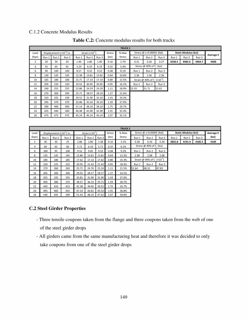
149

C.1.2 Concrete Modulus Results

Table C.2: Concrete modulus results for both trucks

Run 1 Run 2 Run 3 Run 1 Run 2 Run 3 Run 1 Run 2 Run 3 Run 1 Run 2 Run 3

2 20 30 20 1.90 2.86 1.90 0.16 2.7% 0.31 0.26 0.27 4238.4 4482.6 4464.7 4400

4 55 65 65 5.24 6.19 6.19 0.32 5.4%

6 90 100 100 8.57 9.52 9.52 0.48 8.1% Run 1 Run 2 Run 3

8 130 145 145 12.38 13.81 13.81 0.64 10.8% 2.36 2.36 2.36

10 165 180 180 15.71 17.14 17.14 0.80 13.5%

12 205 220 220 19.52 20.95 20.95 0.95 16.2% Run 1 Run 2 Run 3

14 240 255 255 22.86 24.29 24.29 1.11 18.9% 53.33 51.71 51.62

16 270 300 295 25.71 28.57 28.10 1.27 21.6%

18 310 335 330 29.52 31.90 31.43 1.43 24.3%

20 345 370 370 32.86 35.24 35.24 1.59 27.0%

22 390 400 400 37.14 38.10 38.10 1.75 29.7%

24 425 440 440 40.48 41.90 41.90 1.91 32.4%

26 475 475 475 45.24 45.24 45.24 2.07 35.1%

Stress @ ε=0.00005 (ksi) Static Modulus (ksi)Average E

Stress @ 40% of fc' (ksi)

Strain @ 40% of fc' (×10-5

)

TRUCK 1

Load

(kips)

Displacement (×10-5

) in. Strain (×10-5

) Stress

(ksi)

% Max

Stress

Run 1 Run 2 Run 3 Run 1 Run 2 Run 3 Run 1 Run 2 Run 3 Run 1 Run 2 Run 3

2 30 30 25 2.86 2.86 2.38 0.16 3.1% 0.28 0.26 0.28 3855.8 4191.9 4185.5 4100

4 60 65 60 5.71 6.19 5.71 0.32 6.1%

6 100 95 100 9.52 9.05 9.52 0.48 9.2% Run 1 Run 2 Run 3

8 135 145 145 12.86 13.81 13.81 0.64 12.3% 2.08 2.08 2.08

10 185 180 185 17.62 17.14 17.62 0.80 15.3%

12 220 225 225 20.95 21.43 21.43 0.95 18.4% Run 1 Run 2 Run 3

14 270 260 265 25.71 24.76 25.24 1.11 21.5% 51.64 48.31 47.83

16 305 300 300 29.05 28.57 28.57 1.27 24.5%

18 355 335 335 33.81 31.90 31.90 1.43 27.6%

20 405 380 375 38.57 36.19 35.71 1.59 30.7%

22 445 410 415 42.38 39.05 39.52 1.75 33.7%

24 495 460 455 47.14 43.81 43.33 1.91 36.8%

26 540 505 500 51.43 48.10 47.62 2.07 39.8%

Static Modulus (ksi) Average E

(ksi)

Stress @ 40% of fc' (ksi)

Strain @ 40% of fc' (×10-5

)

TRUCK 2

Load

(kips)

Displacement (×10-5

) in. Strain (×10-5

) Stress

(ksi)

% Max

Stress

Stress @ ε=0.00005 (ksi)

C.2 Steel Girder Properties

- Three tensile coupons taken from the flange and three coupons taken from the web of one

of the steel girder drops

- All girders came from the same manufacturing heat and therefore it was decided to only

take coupons from one of the steel girder drops

150

Table C.3: Steel girder coupon tensile test results

Flange 1 0.8376 48.17 57.51 61.5 73.42

Flange 2 0.7894 46.55 58.97 61.22 77.55

Flange 3 0.7845 46.05 58.70 60.75 77.44

Web 1 0.5598 33.25 59.40 41.4 73.95

Web 2 0.5905 36.34 61.54 44.94 76.10

Web 3 0.5599 35.66 63.69 42.79 76.42

Area (in.2)Sample

Yield Ultimate

Stress

(ksi)

Load

(kips)

Stress

(ksi)

Load

(kips)

C.3 Steel Deck Properties

- Three tensile coupons taken from leftover sections of the steel deck used in the test

specimen

- Values for yield stress given are taken as the 0.2% offset value

- Values for ultimate stress given are the maximum stress achieved in each tensile coupon

Table C.4: Steel deck coupon tensile test results

Coupon 1 0.0184 1781.6 96.90 1807.1 98.30

Coupon 2 0.0184 1775.1 96.60 1797.1 97.80

Coupon 3 0.0183 1762.3 96.10 1805.8 98.50

Area (in.2)Sample

Yield Ultimate

Stress

(ksi)

Load

(lbs)

Stress

(ksi)

Load

(lbs)

151

Appendix D: Steel Deck Form as Lateral Bracing Background Calculations

D.1 Bracing Lateral Stiffness

D.1.1 Steel Deck Form Stiffness Requirements

- Calculations provided are for the test specimen, not the design bridge

- Load and resistance factors are included to provide a conservative result for design

- Required effective shear modulus for steel deck form (diaphragm)

( )d

gbu

sdm

MCMG

φ

*

'

dreq'

4 −=

( ) wy

b

g

yg

b

g CIL

EJGIE

LM

2

+=

ππφ

( )( )

( )( )( )( )[ ]( )( )

( )( )25709.243012

2900014.185.111539.2429000

30129.0

2

+

=

ππgM

=gM 905.41 in.-kip

=bC 1.14 (assumed for uniform loading)

===4.1

14.1

4.1

* bb

CC 0.814

=m 0.5

=d 20.8 in.

=ds (7 ft)(12) = 84 in.

( )( )[ ] =

=

8

11230

12

043.125.1

2

uM 1760.06 in.-kip

( )( )[ ]( )( )( )

=−

=848.205.075.0

41.905814.006.17604'

dreq'G 6.25 kip/in./rad

D.1.2 Steel Deck Form Stiffness Provided

- Form is 20 gage Strongweb provided by Wheeling Corrugating

- All formulas and values taken from the Steel Deck Institute Diaphragm Design Manual

(2004)

152

l

S

Snn

Sw

tEC

s

f

sp

f

++

=

22

2

21 αα

= Slip Coefficient

=E steel deck modulus of elasticity = 29500 ksi

=t steel deck thickness = 0.0395 in.

=w steel deck cover width = 32 in.

=l panel length = 14 ft

=fS structural connector flexibility = 0359.01000

15.1

1000

15.1=

t = 0.006069 in./kip

=sS side-lap connector flexibility = 0359.01000

0.3

1000

0.3=

t = 0.015833 in./kip

=1α end distribution factor = ( )

32

)16(282 +=

∑w

xe = 1.5

- ex = distance from panel centerline to any fastener at the end support

=pn number of purloins excluding those at ends = 0

=sn number of stitch connectors within length l = 5

- Taken here as the number of stitch connectors between supports

( ) ( )( ) ( )

( )( )1214

015833.0

006069.05205.12

2006069.0

32

0359.029500

++

=C = 9.877

Cl

D

d

s

EtG

v

xx ++

=3.0

6.2

'

( ) ( ) 1.45.2122 2 ++=++= fwes = 11.1 in.

- values for e, w2, and f measured from drawings of the steel deck cross-section

d = deck pitch = 8 in.

xxD = steel deck warping constant = 400

- estimate based on number of end fasteners deck profiles of similar geometries

vl = distance between supports = 7 ft

153

( )( )

877.97

4003.0

8

1.116.2

0359.029500'

++

=G = 34.58 kip/in.

D.2 Bracing Lateral Strength

D.2.1 Steel Deck Form Connector Strength Requirements

- Strength requirements are based on a 5 edge fastener pattern over the cover width of 32 in.

- Correction factor for strength

=

+=

+=

58.34

25.6

4

1

4

3

4

1

4

3'

'

'

prov

dreq

rG

GC 0.795

-Brace moment per unit length

( )( )( )( )===

22

'

8.20

795.0123006.1760001.0001.0

d

LCMM ru

br 1.164 in.-kips/in.

- Component of brace force perpendicular to beam longitudinal axis

=====25.1

164.1

25.125.125.1

''

br

d

dbr

d

br

M

M

w

wM

w

MF 0.931 kips

- Component of brace force parallel to beam longitudinal axis

( )( )( )( )

==

=

5845

32164.12

5

2'

ed

dbr

VnL

wMF 0.035 kips

- Critical resultant load on a single shear connector

( ) ( ) ( ) ( ) =+=+=2222

035.0931.0VMR FFF 0.932 kips

D.2.1 Steel Deck Form Connector Strength Provided

- Strength of shear connector weld – Salmon and Johnson (1996)

( )( ) === 656013.0uscn fAQ 39.08 kips

- Bearing and tear-out strength of steel deck form

Values calculated for the one stud per rib location because this is the more critical layout

( )( )( ) === 0.980359.0875.04.24.2 un dtFR 7.39 kips

- Bearing and tear-out controls

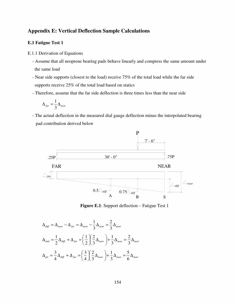
154

Appendix E: Vertical Deflection Sample Calculations

E.1 Fatigue Test 1

E.1.1 Derivation of Equations

- Assume that all neoprene bearing pads behave linearly and compress the same amount under

the same load

- Near side supports (closest to the load) receive 75% of the total load while the far side

supports receive 25% of the total load based on statics

- Therefore, assume that the far side deflection is three times less than the near side

nearfar ∆=∆3

1

- The actual deflection in the measured dial gauge deflection minus the interpolated bearing

pad contribution derived below

near

.25P

P

.75P30' - 0"

7' - 6"

0.5 0.75

far

diffdiff

diff

FAR NEAR

A B S

Figure E.1: Support deflection – Fatigue Test 1

nearnearnearfarneardiff ∆=∆−∆=∆−∆=∆3

2

3

1

nearnearnearfardiffmid ∆=∆+

∆

=∆+∆=∆

3

2

3

1

3

2

2

1

2

1

nearnearnearfardiffqtr ∆=∆+

∆

=∆+∆=∆

6

5

3

1

3

2

4

3

4

3

155

E.1.2 Mid-Span Sample Calculation

- Data is taken from DG 1-A at 500,000 cycles, Static Test #1

1-A value at 1 kip = 0.1872 in.


=−=∆ − 1872.03563.01 A 0.1691 in.

S-1 value at 1 kip = 0.5471 in.


=−=∆ 4963.05471.0near 0.0508 in.

=

=∆=∆ 0508.0

3

2

3

2nearmid 0.0339 in.

=−=∆ − 0339.01691.0,1 adjA 0.1352 in.

E.1.3 Quarter-Span Sample Calculation

- Data is taken from DG 1-B at 500,000 cycles, Static Test #1

1-B value at 1 kip = 0.0288 in.


=−=∆ − 0288.01896.01 B 0.1608 in.



=−=∆ 4963.05471.0near 0.0508 in.

=

=∆=∆ 0508.0

6

5

6

5nearmid 0.0423 in.

=−=∆ − 0423.01608.0,1 adjB 0.1185 in.

E.2 Fatigue Test 2

E.2.1 Derivation

- Data taken from both supports

- Same process as above, however load is now closer to far side

156

far

.25P

P

.75P 30' - 0"

7' - 6"

0.50.75

near

diffdiff

diff

FARNEAR

ABS

Sb

Figure E.2: Support deflection – Fatigue Test 2

neardiffmid ∆+∆=∆2

1

neardiffqtr ∆+∆=∆4

3

E.2.2 Mid-Span Deflection Calculation

- Data is taken from DG 1-A at 500,000 cycles, Static Test #1



=−=∆ − 2020.05501.01 A 0.3481 in.



=−=∆ 4536.06201.0far 0.1582 in.

S-1b value at 1 kip = 0.3039 in.


=−=∆ 2670.03039.0near 0.0369 in.

( ) =+−

=∆+∆=∆ 0369.00369.01582.0

2

1

2

1neardiffmid 0.0976 in.

=−=∆ − 0976.03481.0,1 adjA 0.2505 in.

157

E.2.2 Quarter-Span Deflection Calculation

- Data is taken from DG 1-B at 500,000 cycles, Static Test #1



=−=∆ − 1424.04861.01 B 0.3437 in.



=−=∆ 4536.06201.0far 0.1582 in.



=−=∆ 2670.03039.0near 0.0369 in.

( ) =+−

=∆+∆=∆ 0369.00369.01582.0

4

3

4

3neardiffmid 0.1279 in.

=−=∆ − 1279.03437.0,1 adjB 0.2158 in.

158

Appendix F: Fatigue Testing Results

F.1 Fatigue Test 1

F.1.1 Deflection Results

Table F.1: Deflection results for Girders 1 and 2 in Fatigue Test 1

Cycle DG 1-A DG 1-B DG 2-A DG 2-B

1 Deflection (in.) -0.1316 -0.1148 -0.1309 -0.1147

% Change 0.00% 0.00% 0.00% 0.00%

10 Deflection (in.) -0.1328 -0.1151 -0.1314 -0.1152

% Change 0.90% 0.34% 0.38% 0.40%

100 Deflection (in.) -0.1322 -0.1148 -0.1313 -0.1154

% Change 0.46% 0.00% 0.37% 0.58%

1000 Deflection (in.) -0.1326 -0.1148 -0.1315 -0.1153

% Change 0.76% 0.04% 0.51% 0.53%

10000 Deflection (in.) -0.1337 -0.1156 -0.1329 -0.1158

% Change 1.56% 0.76% 1.57% 0.96%

50000 Deflection (in.) -0.1324 -0.1157 -0.1335 -0.1160

% Change 0.61% 0.79% 1.98% 1.15%

100000 Deflection (in.) -0.1333 -0.1166 -0.1348 -0.1161

% Change 1.27% 1.58% 3.00% 1.22%

200000 Deflection (in.) -0.1329 -0.1161 -0.1356 -0.1175

% Change 0.95% 1.21% 3.63% 2.44%

300000 Deflection (in.) -0.1342 -0.1171 -0.1362 -0.1177

% Change 1.93% 2.08% 4.06% 2.58%

400000 Deflection (in.) -0.1346 -0.1177 -0.1368 -0.1183

% Change 2.25% 2.55% 4.51% 3.10%

500000 Deflection (in.) -0.1352 -0.1184 -0.1367 -0.1189

% Change 2.69% 3.17% 4.46% 3.64%

600000 Deflection (in.) -0.1359 -0.1192 -0.1377 -0.1194

% Change 3.21% 3.85% 5.19% 4.08%

700000 Deflection (in.) -0.1376 -0.1201 -0.1381 -0.1195

% Change 4.57% 4.69% 5.50% 4.18%

800000 Deflection (in.) -0.1370 -0.1193 -0.1384 -0.1204

% Change 4.05% 3.95% 5.73% 4.93%

900000 Deflection (in.) -0.1374 -0.1199 -0.1371 -0.1205

% Change 4.38% 4.44% 4.76% 5.00%

1000000 Deflection (in.) -0.1370 -0.1200 -0.1381 -0.1209

% Change 4.08% 4.58% 5.54% 5.41%

1150000 Deflection (in.) -0.1375 -0.1205 -0.1387 -0.1223

% Change 4.42% 4.97% 5.98% 6.57%

1200000 Deflection (in.) -0.1382 -0.1208 -0.1397 -0.1230

% Change 4.99% 5.30% 6.77% 7.25%

159

F.1.2 Slip Results

Table F.2: Interface slip results for Girders 1 and 2 in Fatigue Test 1

Cycle DG 1-A LVDT 1-B LVDT 1-C LVDT 2-A LVDT 2-B LVDT 2-C

1 Slip (in.) -0.0011 -0.0015 -0.0011 -0.0011 -0.0016 -0.0013

% Change 0.00% 0.00% 0.00% 0.00% 0.00% 0.00%

10 Slip (in.) -0.0013 -0.0015 -0.0011 -0.0011 -0.0016 -0.0013

% Change 17.65% 0.23% -2.75% -2.63% -1.66% 0.00%

100 Slip (in.) -0.0013 -0.0014 -0.0011 -0.0011 -0.0016 -0.0013

% Change 14.71% -1.82% -2.75% -1.75% -0.83% 0.00%

1000 Slip (in.) -0.0012 -0.0015 -0.0011 -0.0011 -0.0016 -0.0013

% Change 8.82% 0.91% -0.31% -6.14% -0.42% 0.00%

10000 Slip (in.) -0.0012 -0.0016 -0.0012 -0.0011 -0.0017 -0.0014

% Change 8.82% 8.41% 11.01% 0.58% 6.03% 9.52%

50000 Slip (in.) -0.0012 -0.0016 -0.0013 -0.0012 -0.0017 -0.0014

% Change 8.82% 9.09% 16.51% 4.39% 7.48% 14.29%

100000 Slip (in.) -0.0011 -0.0016 -0.0012 -0.0012 -0.0017 -0.0014

% Change 0.00% 8.41% 11.01% 8.77% 4.99% 7.14%

200000 Slip (in.) -0.0012 -0.0016 -0.0012 -0.0012 -0.0017 -0.0014

% Change 5.88% 7.73% 7.95% 8.48% 8.52% 7.14%

300000 Slip (in.) -0.0011 -0.0016 -0.0012 -0.0013 -0.0018 -0.0015

% Change -5.88% 8.64% 14.37% 12.28% 13.31% 15.87%

400000 Slip (in.) -0.0011 -0.0016 -0.0012 -0.0013 -0.0019 -0.0015

% Change -2.94% 9.32% 12.84% 11.40% 20.17% 16.67%

500000 Slip (in.) -0.0011 -0.0016 -0.0013 -0.0013 -0.0020 -0.0015

% Change -2.94% 10.23% 16.51% 11.40% 23.28% 21.43%

600000 Slip (in.) -0.0011 -0.0017 -0.0012 -0.0013 -0.0021 -0.0016

% Change 0.00% 12.95% 12.84% 11.40% 29.31% 28.57%

700000 Slip (in.) -0.0011 -0.0017 -0.0013 -0.0013 -0.0022 -0.0017

% Change 0.00% 13.18% 16.51% 14.91% 37.01% 35.71%

800000 Slip (in.) -0.0013 -0.0017 -0.0013 -0.0014 -0.0024 -0.0020

% Change 14.71% 15.91% 22.02% 21.35% 49.06% 54.76%

900000 Slip (in.) -0.0013 -0.0017 -0.0013 -0.0014 -0.0025 -0.0021

% Change 17.65% 18.18% 19.27% 19.88% 56.96% 69.05%

1000000 Slip (in.) -0.0013 -0.0018 -0.0013 -0.0014 -0.0026 -0.0022

% Change 11.76% 20.45% 22.02% 19.30% 60.50% 71.43%

1150000 Slip (in.) -0.0014 -0.0019 -0.0014 -0.0015 -0.0028 -0.0025

% Change 26.47% 26.14% 30.28% 33.92% 75.68% 96.03%

1200000 Slip (in.) -0.0016 -0.0019 -0.0014 -0.0016 -0.0029 -0.0027

% Change 38.24% 29.55% 30.28% 38.60% 81.29% 110.32%

160

F.1.3 Strain Results

Table F.3: Strain gauge results for Girder 1 in Fatigue Test 1

Cycle SG 1-1 SG 1-2 SG 1-3 SG 1-4 SG 1-5 SG 1-6 SG 1-7

1 Strain (µε) 270.4 203.4 147.0 90.1 25.6 208.8 151.1

% Change 0.00% 0.00% 0.00% 0.00% 0.00% 0.00% 0.00%

10 Strain (µε) 270.6 204.2 147.6 90.4 27.2 210.2 152.3

% Change 0.06% 0.39% 0.44% 0.35% 6.21% 0.68% 0.84%

100 Strain (µε) 270.9 204.2 147.8 90.2 26.2 210.2 152.0

% Change 0.18% 0.39% 0.54% 0.17% 2.49% 0.69% 0.63%

1000 Strain (µε) 270.4 203.7 147.1 90.2 26.2 210.4 151.7

% Change 0.00% 0.16% 0.11% 0.17% 2.47% 0.76% 0.42%

10000 Strain (µε) 272.8 204.2 147.0 89.4 22.3 210.2 151.4

% Change 0.88% 0.39% 0.00% -0.71% -13.07% 0.69% 0.21%

50000 Strain (µε) 271.9 203.6 146.2 88.3 21.3 209.4 150.4

% Change 0.53% 0.08% -0.54% -1.94% -16.78% 0.30% -0.42%

100000 Strain (µε) 274.1 205.0 147.0 88.3 20.4 211.0 151.7

% Change 1.35% 0.78% 0.00% -1.94% -20.50% 1.06% 0.42%

200000 Strain (µε) 273.9 204.5 146.5 87.5 20.0 210.5 151.7

% Change 1.30% 0.55% -0.32% -2.82% -21.75% 0.84% 0.42%

300000 Strain (µε) 275.7 206.1 147.3 87.7 19.4 211.8 151.9

% Change 1.94% 1.33% 0.22% -2.65% -24.24% 1.45% 0.53%

400000 Strain (µε) 277.6 207.2 147.8 88.1 18.9 212.9 152.8

% Change 2.65% 1.88% 0.54% -2.13% -26.11% 1.98% 1.16%

500000 Strain (µε) 279.2 208.8 148.9 88.6 19.1 214.7 153.8

% Change 3.23% 2.66% 1.30% -1.59% -25.46% 2.82% 1.79%

600000 Strain (µε) 280.1 209.6 149.0 88.8 18.8 215.3 154.1

% Change 3.59% 3.05% 1.41% -1.42% -26.75% 3.12% 2.00%

700000 Strain (µε) 281.6 210.2 149.7 88.8 18.1 216.1 154.9

% Change 4.12% 3.37% 1.84% -1.42% -29.21% 3.51% 2.52%

800000 Strain (µε) 281.1 209.8 149.3 88.5 17.5 215.8 154.7

% Change 3.94% 3.13% 1.62% -1.77% -31.71% 3.35% 2.42%

900000 Strain (µε) 280.9 209.6 148.9 87.8 17.0 215.6 154.6

% Change 3.88% 3.05% 1.30% -2.48% -33.55% 3.27% 2.31%

1000000 Strain (µε) 281.6 209.6 149.0 88.0 16.9 215.8 153.9

% Change 4.12% 3.05% 1.41% -2.30% -34.17% 3.35% 1.89%

1150000 Strain (µε) 283.0 211.0 149.8 88.0 16.7 217.0 155.2

% Change 4.64% 3.75% 1.95% -2.31% -34.79% 3.95% 2.73%

1200000 Strain (µε) 283.3 210.6 149.5 87.7 16.4 216.7 154.4

% Change 4.76% 3.52% 1.73% -2.65% -36.04% 3.80% 2.20%

161



1 Strain (µε) 283.5 210.5 160.0 92.9 23.9 214.6 154.4

% Change 0.00% 0.00% 0.00% 0.00% 0.00% 0.00% 0.00%

10 Strain (µε) 284.0 211.3 160.2 93.4 23.9 214.9 155.8

% Change 0.17% 0.38% 0.10% 0.52% 0.00% 0.15% 0.93%

100 Strain (µε) 284.0 210.9 160.4 93.5 23.6 215.1 155.6

% Change 0.17% 0.16% 0.20% 0.68% -1.34% 0.22% 0.82%

1000 Strain (µε) 284.0 211.3 160.0 93.5 23.0 215.4 155.6

% Change 0.17% 0.38% 0.00% 0.69% -3.99% 0.37% 0.82%

10000 Strain (µε) 285.4 212.1 160.5 92.2 20.7 216.0 155.2

% Change 0.68% 0.76% 0.30% -0.69% -13.34% 0.67% 0.52%

50000 Strain (µε) 285.7 212.0 160.0 91.4 20.1 216.0 154.7

% Change 0.79% 0.69% 0.00% -1.54% -16.01% 0.67% 0.21%

100000 Strain (µε) 289.7 214.2 161.5 92.1 19.6 218.6 156.4

% Change 2.20% 1.74% 0.90% -0.86% -18.00% 1.86% 1.34%

200000 Strain (µε) 289.7 214.4 161.3 91.8 19.6 218.6 156.0

% Change 2.20% 1.82% 0.80% -1.20% -18.02% 1.86% 1.03%

300000 Strain (µε) 292.3 215.5 161.8 91.6 17.5 219.7 156.6

% Change 3.10% 2.35% 1.10% -1.37% -26.67% 2.38% 1.44%

400000 Strain (µε) 293.7 216.4 162.4 91.4 16.6 220.8 157.4

% Change 3.61% 2.81% 1.49% -1.55% -30.69% 2.90% 1.95%

500000 Strain (µε) 295.5 217.4 163.4 91.6 16.9 221.8 157.9

% Change 4.23% 3.26% 2.09% -1.37% -29.35% 3.35% 2.27%

600000 Strain (µε) 296.0 218.2 163.1 91.6 16.4 222.3 158.0

% Change 4.40% 3.63% 1.89% -1.37% -31.35% 3.57% 2.36%

700000 Strain (µε) 297.1 218.5 163.4 90.8 15.3 222.8 157.7

% Change 4.80% 3.79% 2.09% -2.24% -35.99% 3.80% 2.16%

800000 Strain (µε) 295.3 217.2 161.6 89.4 14.8 220.8 156.4

% Change 4.17% 3.18% 0.99% -3.78% -38.02% 2.90% 1.33%

900000 Strain (µε) 295.6 216.6 161.1 88.3 14.3 220.5 155.6

% Change 4.29% 2.88% 0.69% -4.98% -40.02% 2.76% 0.82%

1000000 Strain (µε) 294.9 216.0 160.4 88.1 13.2 220.0 155.0

% Change 4.01% 2.58% 0.20% -5.15% -44.69% 2.53% 0.41%

1150000 Strain (µε) 298.4 218.0 160.8 86.5 8.8 221.6 155.3

% Change 5.24% 3.56% 0.49% -6.88% -63.32% 3.27% 0.61%

1200000 Strain (µε) 298.7 217.7 160.2 85.4 7.8 221.5 155.2

% Change 5.36% 3.41% 0.09% -8.07% -67.34% 3.20% 0.51%

162

Table F.5: Calculated elastic neutral axis for Girders 1 and 2 in Fatigue Test 1

Cycle GIRDER 1 GIRDER 2

1 ENA (in.) 22.38 22.19

% Change 0.00% 0.00%

10 ENA (in.) 22.49 22.20

% Change 0.51% 0.07%

100 ENA (in.) 22.42 22.19

% Change 0.19% 0.01%

1000 ENA (in.) 22.43 21.96

% Change 0.21% -1.03%

10000 ENA (in.) 22.11 21.82

% Change -1.21% -1.66%

50000 ENA (in.) 22.03 21.89

% Change -1.57% -1.36%

100000 ENA (in.) 21.94 21.82

% Change -1.97% -1.66%

200000 ENA (in.) 21.90 21.80

% Change -2.17% -1.73%

300000 ENA (in.) 21.83 21.65

% Change -2.45% -2.43%

400000 ENA (in.) 21.79 21.58

% Change -2.63% -2.75%

500000 ENA (in.) 21.80 21.57

% Change -2.61% -2.77%

600000 ENA (in.) 21.77 21.54

% Change -2.75% -2.92%

700000 ENA (in.) 21.71 21.44

% Change -2.98% -3.37%

800000 ENA (in.) 21.68 21.39

% Change -3.15% -3.61%

900000 ENA (in.) 21.63 21.31

% Change -3.36% -3.93%

1000000 ENA (in.) 21.61 21.26

% Change -3.44% -4.17%

1150000 ENA (in.) 21.59 20.95

% Change -3.55% -5.57%

1200000 ENA (in.) 21.55 20.87

% Change -3.73% -5.95%

163

F.2 Fatigue Test 2

F.2.1 Deflection Results

Table F.6: Deflection results for Girders 1 and 2 in Fatigue Test 2

Cycle DG 1-A DG 1-B DG 2-A DG 2-B

1 Deflection (in.) -0.2476 -0.2106 -0.2566 -0.2168

% Change 0.00% 0.00% 0.00% 0.00%

10 Deflection (in.) -0.2477 -0.2110 -0.2537 -0.2153

% Change 0.03% 0.15% -1.11% -0.71%

100 Deflection (in.) -0.2477 -0.2113 -0.2565 -0.2169

% Change 0.04% 0.32% -0.02% 0.02%

1000 Deflection (in.) -0.2481 -0.2116 -0.2592 -0.2185

% Change 0.20% 0.47% 1.01% 0.80%

10000 Deflection (in.) -0.2525 -0.2161 -0.2584 -0.2233

% Change 1.99% 2.60% 0.70% 3.01%

50000 Deflection (in.) -0.2548 -0.2192 -0.2590 -0.2256

% Change 2.93% 4.05% 0.95% 4.06%

100000 Deflection (in.) -0.2591 -0.2230 -0.2697 -0.2330

% Change 4.65% 5.88% 5.09% 7.45%

200000 Deflection (in.) -0.2537 -0.2185 -0.2654 -0.2291

% Change 2.48% 3.71% 3.45% 5.68%

300000 Deflection (in.) -0.2509 -0.2157 -0.2628 -0.2273

% Change 1.33% 2.43% 2.43% 4.84%

400000 Deflection (in.) -0.2512 -0.2163 -0.2644 -0.2288

% Change 1.45% 2.71% 3.03% 5.53%

500000 Deflection (in.) -0.2508 -0.2158 -0.2647 -0.2291

% Change 1.29% 2.46% 3.17% 5.67%

600000 Deflection (in.) -0.2531 -0.2178 -0.2665 -0.2312

% Change 2.24% 3.41% 3.85% 6.65%

700000 Deflection (in.) -0.2541 -0.2188 -0.2671 -0.2313

% Change 2.65% 3.85% 4.10% 6.67%

800000 Deflection (in.) -0.2553 -0.2207 -0.2671 -0.2319

% Change 3.10% 4.77% 4.09% 6.96%

900000 Deflection (in.) -0.2530 -0.2185 -0.2656 -0.2308

% Change 2.19% 3.71% 3.51% 6.45%

1000000 Deflection (in.) -0.2600 -0.2247 -0.2727 -0.2372

% Change 5.01% 6.68% 6.28% 9.41%

1100000 Deflection (in.) -0.2586 -0.2236 -0.2708 -0.2366

% Change 4.44% 6.17% 5.52% 9.14%

1200000 Deflection (in.) -0.2593 -0.2247 -0.2710 -0.2371

% Change 4.74% 6.69% 5.63% 9.37%

164

F.2.2 Slip Results

Table F.7: Interface slip results for Girders 1 and 2 in Fatigue Test 2

Cycle LVDT 1-A LVDT 1-B LVDT 1-C LVDT 2-A LVDT 2-B LVDT 2-C

1 Slip (in.) -0.0006 -0.0022 -0.0019 -0.0010 -0.0023 -0.0025

% Change 0.00% 0.00% 0.00% 0.00% 0.00% 0.00%

10 Slip (in.) -0.0007 -0.0022 -0.0019 -0.0010 -0.0024 -0.0026

% Change 5.79% 1.06% -0.69% 3.01% 3.17% 1.31%

100 Slip (in.) -0.0006 -0.0022 -0.0021 -0.0010 -0.0024 -0.0026

% Change 1.58% 0.30% 6.22% 0.00% 1.59% 2.49%

1000 Slip (in.) -0.0007 -0.0023 -0.0023 -0.0010 -0.0025 -0.0028

% Change 5.79% 5.30% 17.62% 2.68% 7.78% 9.55%

10000 Slip (in.) -0.0007 -0.0024 -0.0027 -0.0011 -0.0025 -0.0032

% Change 16.84% 9.38% 40.93% 13.71% 9.51% 26.83%

50000 Slip (in.) -0.0008 -0.0022 -0.0031 -0.0013 -0.0025 -0.0036

% Change 29.47% -0.45% 59.59% 32.11% 6.05% 39.79%

100000 Slip (in.) -0.0009 -0.0022 -0.0032 -0.0013 -0.0024 -0.0037

% Change 42.11% -2.42% 64.25% 32.44% 5.48% 44.50%

200000 Slip (in.) -0.0009 -0.0021 -0.0033 -0.0014 -0.0024 -0.0038

% Change 48.42% -4.24% 68.39% 35.45% 3.75% 48.04%

300000 Slip (in.) -0.0009 -0.0021 -0.0034 -0.0014 -0.0024 -0.0039

% Change 48.42% -4.69% 73.58% 39.46% 3.75% 51.57%

400000 Slip (in.) -0.0010 -0.0021 -0.0034 -0.0014 -0.0026 -0.0040

% Change 50.00% -2.87% 78.24% 43.48% 10.23% 55.10%

500000 Slip (in.) -0.0010 -0.0022 -0.0036 -0.0015 -0.0026 -0.0041

% Change 50.53% 0.15% 85.84% 47.83% 13.69% 62.17%

600000 Slip (in.) -0.0010 -0.0023 -0.0037 -0.0015 -0.0028 -0.0043

% Change 56.84% 5.14% 90.67% 50.50% 20.03% 69.24%

700000 Slip (in.) -0.0010 -0.0024 -0.0039 -0.0016 -0.0029 -0.0044

% Change 61.05% 9.38% 101.55% 57.19% 26.22% 73.95%

800000 Slip (in.) -0.0011 -0.0025 -0.0042 -0.0016 -0.0033 -0.0047

% Change 71.58% 13.16% 115.89% 59.53% 42.22% 85.73%

900000 Slip (in.) -0.0011 -0.0026 -0.0045 -0.0017 -0.0037 -0.0050

% Change 73.68% 18.76% 131.61% 68.23% 59.08% 97.51%

1000000 Slip (in.) -0.0012 -0.0028 -0.0048 -0.0017 -0.0040 -0.0054

% Change 86.32% 27.23% 147.15% 66.89% 72.48% 110.47%

1100000 Slip (in.) -0.0012 -0.0032 -0.0053 -0.0018 -0.0044 -0.0057

% Change 96.84% 44.33% 173.58% 75.92% 88.04% 124.61%

1200000 Slip (in.) -0.0013 -0.0034 -0.0057 -0.0018 -0.0047 -0.0061

% Change 111.58% 56.13% 195.34% 80.60% 101.01% 139.92%

165

F.2.3 Strain Results



1 Strain (µε) 515.6 404.3 292.0 177.2 38.0 392.0 295.0

% Change 0.00% 0.00% 0.00% 0.00% 0.00% 0.00% 0.00%

10 Strain (µε) 516.2 404.1 291.8 176.8 36.9 392.3 295.0

% Change 0.12% -0.04% -0.05% -0.18% -2.94% 0.08% 0.00%

100 Strain (µε) 516.5 404.8 292.8 176.8 36.2 392.1 295.2

% Change 0.19% 0.12% 0.27% -0.18% -4.61% 0.04% 0.06%

1000 Strain (µε) 517.5 404.3 290.6 174.8 32.6 392.0 294.2

% Change 0.38% 0.00% -0.49% -1.35% -14.23% 0.00% -0.27%

10000 Strain (µε) 524.4 408.6 292.6 173.5 25.9 396.4 296.0

% Change 1.71% 1.07% 0.22% -2.06% -31.80% 1.14% 0.32%

50000 Strain (µε) 529.3 411.3 293.1 171.9 20.5 398.5 296.3

% Change 2.67% 1.74% 0.38% -2.97% -46.03% 1.67% 0.43%

100000 Strain (µε) 536.2 416.6 296.3 172.9 19.2 403.9 300.1

% Change 4.01% 3.04% 1.47% -2.43% -49.37% 3.05% 1.73%

200000 Strain (µε) 523.9 406.5 287.9 167.5 17.2 393.9 292.2

% Change 1.62% 0.55% -1.42% -5.48% -54.83% 0.49% -0.97%

300000 Strain (µε) 518.6 401.7 286.0 165.5 17.2 389.6 287.9

% Change 0.60% -0.63% -2.07% -6.55% -54.81% -0.61% -2.42%

400000 Strain (µε) 517.6 400.9 284.4 163.6 15.3 388.6 287.1

% Change 0.40% -0.83% -2.62% -7.64% -59.84% -0.86% -2.69%

500000 Strain (µε) 516.7 399.8 283.1 162.8 14.3 387.2 286.1

% Change 0.22% -1.11% -3.06% -8.08% -62.34% -1.22% -3.02%

600000 Strain (µε) 521.0 403.2 284.7 162.8 14.0 390.4 287.7

% Change 1.06% -0.27% -2.50% -8.08% -63.19% -0.40% -2.47%

700000 Strain (µε) 522.1 403.8 285.2 162.2 12.9 391.3 287.9

% Change 1.28% -0.12% -2.34% -8.44% -66.12% -0.16% -2.42%

800000 Strain (µε) 524.1 405.2 285.0 161.1 9.7 392.3 287.9

% Change 1.65% 0.24% -2.40% -9.07% -74.48% 0.08% -2.43%

900000 Strain (µε) 517.6 399.7 280.1 157.3 7.2 386.8 283.4

% Change 0.41% -1.15% -4.09% -11.23% -81.18% -1.30% -3.93%

1000000 Strain (µε) 531.3 409.3 287.9 161.6 7.5 396.7 290.3

% Change 3.05% 1.23% -1.41% -8.80% -80.33% 1.22% -1.61%

1100000 Strain (µε) 528.9 407.3 285.0 158.2 3.7 394.4 287.7

% Change 2.59% 0.76% -2.39% -10.69% -90.38% 0.62% -2.47%

1200000 Strain (µε) 533.0 409.4 284.5 156.0 -1.4 396.3 287.9

% Change 3.39% 1.26% -2.56% -11.94% -103.76% 1.10% -2.42%

166



1 Strain (µε) 533.2 408.9 303.7 195.3 44.7 401.3 294.7

% Change 0.00% 0.00% 0.00% 0.00% 0.00% 0.00% 0.00%

10 Strain (µε) 533.4 409.4 303.9 195.0 44.4 401.7 294.8

% Change 0.03% 0.12% 0.05% -0.16% -0.71% 0.12% 0.05%

100 Strain (µε) 534.6 409.5 304.4 195.0 43.6 402.1 295.0

% Change 0.27% 0.16% 0.21% -0.16% -2.50% 0.20% 0.11%

1000 Strain (µε) 536.3 410.0 304.2 194.4 40.1 402.9 295.0

% Change 0.57% 0.28% 0.16% -0.49% -10.32% 0.40% 0.11%

10000 Strain (µε) 545.4 416.9 306.8 193.6 34.2 408.6 297.8

% Change 2.29% 1.96% 1.00% -0.90% -23.48% 1.83% 1.08%

50000 Strain (µε) 550.2 419.0 307.3 190.8 28.9 411.0 298.0

% Change 3.19% 2.47% 1.16% -2.29% -35.24% 2.43% 1.13%

100000 Strain (µε) 558.4 424.9 310.6 192.1 26.7 416.9 301.4

% Change 4.72% 3.92% 2.27% -1.63% -40.20% 3.90% 2.27%

200000 Strain (µε) 546.2 414.8 302.9 186.5 22.9 407.7 294.3

% Change 2.44% 1.45% -0.26% -4.49% -48.75% 1.60% -0.11%

300000 Strain (µε) 542.4 412.0 300.1 183.7 21.9 403.3 291.0

% Change 1.72% 0.75% -1.21% -5.95% -50.90% 0.52% -1.25%

400000 Strain (µε) 542.0 410.7 299.1 182.4 19.6 403.3 290.0

% Change 1.65% 0.43% -1.53% -6.62% -56.23% 0.52% -1.57%

500000 Strain (µε) 540.6 409.1 296.9 180.2 17.6 401.4 287.8

% Change 1.38% 0.04% -2.27% -7.76% -60.51% 0.03% -2.33%

600000 Strain (µε) 544.6 412.3 299.1 180.8 17.2 404.6 290.4

% Change 2.14% 0.83% -1.53% -7.43% -61.56% 0.84% -1.46%

700000 Strain (µε) 546.5 413.2 299.3 180.8 15.1 405.6 290.5

% Change 2.50% 1.06% -1.47% -7.43% -66.19% 1.07% -1.41%

800000 Strain (µε) 548.6 414.3 299.4 179.2 11.4 406.5 290.5

% Change 2.89% 1.33% -1.43% -8.25% -74.38% 1.31% -1.41%

900000 Strain (µε) 542.3 409.4 295.1 175.9 9.2 401.9 286.4

% Change 1.72% 0.12% -2.85% -9.96% -79.37% 0.16% -2.82%

1000000 Strain (µε) 558.1 420.9 302.9 180.2 8.3 412.8 293.9

% Change 4.67% 2.94% -0.26% -7.76% -81.50% 2.87% -0.27%

1100000 Strain (µε) 556.0 418.5 300.5 176.7 3.5 410.7 291.5

% Change 4.28% 2.35% -1.05% -9.55% -92.17% 2.35% -1.08%

1200000 Strain (µε) 558.7 420.1 301.0 176.0 -0.9 412.4 292.4

% Change 4.78% 2.74% -0.90% -9.88% -102.13% 2.79% -0.76%

167

Table F.10: Calculated elastic neutral axis for Girders 1 and 2 in Fatigue Test 2

Cycle GIRDER 1 GIRDER 2

1 ENA (in.) 22.22 22.55

% Change 0.00% 0.00%

10 ENA (in.) 22.17 22.53

% Change -0.22% -0.07%

100 ENA (in.) 22.15 22.50

% Change -0.30% -0.24%

1000 ENA (in.) 21.98 22.36

% Change -1.06% -0.86%

10000 ENA (in.) 21.70 22.08

% Change -2.32% -2.08%

50000 ENA (in.) 21.47 21.84

% Change -3.34% -3.15%

100000 ENA (in.) 21.41 21.74

% Change -3.62% -3.61%

200000 ENA (in.) 21.33 21.63

% Change -3.97% -4.09%

300000 ENA (in.) 21.32 21.58

% Change -4.04% -4.32%

400000 ENA (in.) 21.25 21.48

% Change -4.34% -4.75%

500000 ENA (in.) 21.21 21.39

% Change -4.50% -5.14%

600000 ENA (in.) 21.18 21.37

% Change -4.68% -5.25%

700000 ENA (in.) 21.13 21.29

% Change -4.89% -5.57%

800000 ENA (in.) 21.01 21.16

% Change -5.44% -6.18%

900000 ENA (in.) 20.91 21.08

% Change -5.89% -6.54%

1000000 ENA (in.) 20.91 21.03

% Change -5.87% -6.75%

1100000 ENA (in.) 20.76 20.86

% Change -6.53% -7.49%

1200000 ENA (in.) 20.58 20.73

% Change -7.34% -8.08%

168

Appendix G: Test Specimen Strength Calculations

G.1 Additional Strain to Girder Yield

- Stress from construction

=sS Section modulus of steel section = 94.5 in.3 (AISC 2005)

( ) ( ) 50712

1

2

5.28150concrete +

+=w = 0.8594 lb/ft

=qtrM Moment at the quarter point = ( )( )

==32

308594.03

32

322

wL72.51 kip-ft =870.14 in.-kip

5.94

14.870==

S

qtr

qtrS

Mσ = 9.21 ksi

- Additional strain to yield

=yf 60.0 ksi (from material tests, see “Appendix C”)

Assume a steel modulus of elasticity Es = 29000 ksi

21.90.60 −=−= qtryrem f σσ = 50.79 ksi

29000

79.50==

S

remrem

E

σε = 0.001751 = 1751 µs

G.2 Plastic Moment Capacity Calculations

G.2.1 One Stud-Per-Rib Stud Layout

- Static strength of shear studs (Qn)

uscgpccscn FARREfAQ ≤= '5.0

22

2

875.0

2

=

= ππ sc

sc

dA =0.6013 in.

2

'

cf = 5.80 ksi (from material testing, see “Appendix C”)

Ec = 4400 ksi (from material testing, see “Appendix C”)

Rp = 0.6 (weak side stud placement, AISC 2005)

Rg = 1.0 (one stud per rib, AISC 2005)

( ) ( )( )44008.56013.5.05.0 ' =ccsc EfA = 48.03 kips

169

( )( )( )( )656013.00.16.0=uscgp FARR = 23.45 kips Controls

=nQ 23.45 kip

( )45.2312=∑ nQ = 281.4 kips

- Maximum horizontal load (Fmax)

( ) ( )yscc fAAfTCF ,85.0min,min '

max ==

( )( )( )8848.585.0=C = 3313 kips

( )( )0.607.14=T = 882 kips Controls

maxF = 882 kips > ∑ nQ = 281.4 kips ∴Part of the steel section is in compression

- Calculation of Plastic Moment

nnnx TCCF =+→=∑ 210

221 nysnn CfACC −=+

( )fy

nys

n bafCfA

C 1

1

22

=−

=

W21x50

Deck

Ribs

C

C

n1

n2

Tn

StressSection

Figure G.1: Plastic stress distribution, one stud-per-rib

As = area of steel beam = 14.7 in.2

bf = thickness of beam flange = 6.53 in.

a1 = depth of compression block into steel beam top flange

C1 = compression force in concrete deck

170

( )( )in.535.0.in766.0

53.660

2

4.281882

2

1

1 =>=

−

=

−

= f

fy

nys

tbf

CfA

a

∴ Part of the beam web is in compression

WT10.5x25 Section Properties:

A = 7.36 in.2, tw = 0.380 in., d = 10.4 in., y = 2.93 in.

( ) ( )( )0.6036.7=WTys fA = 441.6 kips

2

4.2818822

−=nC = 300.3 kips < ( )

WTys fA ∴Not all of top WT is in compression

( ) 6.4413.3004.28121 −+=−+=WTysnnweb fACCP = 140.1 kips

webP = total force in the portion of the to WT web that is in tension

ta = depth of top WT web in tension = ( )( )38.00.60

1.140=

wy

web

tf

P = 6.14 in.

=a depth of compression block in concrete deck = ( )( )848.585.0

4.281

85.0 '

1 =ec

n

bf

C = 0.680 in.

Sum moments about the centroid of the top WT section to get Mc1 (calculated capacity)

( ) ( )ydfAa

yd

Pa

yyCM xWWTystxW

webdecknc 222

22

50215021

11 −+

−−+

−+=

( ) ( )[ ]93.228.206.4412

14.693.2

2

8.201.1402

2

68.05.1093.24.2811 −+

−−+

−+=cM

1cM = 11513.9 in-kip = 959.5 ft-kips

( )( )303

5.95916

3

161 ==

L

MP

qtr

c = 170.6 kips

G.2.2 Two Studs-Per-Rib Stud Layout

- Static strength of shear studs (Qn)

uscgpccscn FARREfAQ ≤= '5.0

22

2

875.0

2

=

= ππ sc

sc

dA =0.6013 in.

2

'

cf = 5.20 ksi (Truck 2 from material testing, see “Appendix C”)

Ec = 4100 ksi (Truck 2 from material testing, see “Appendix C”)

Rp = 0.6 (weak side stud placement, AISC 2005)

Rg = 0.85 (two studs per rib, AISC 2005)

171

( ) ( )( )41002.56013.5.05.0 ' =ccsc EfA = 43.90 kips

( )( )( )( )656013.085.06.0=uscgp FARR = 19.93 kips Controls

=nQ 19.93 kip

( )93.1924=∑ nQ = 478.32 kips

- Maximum horizontal load (Fmax)

( ) ( )yscc fAAfTCF ,85.0min,min '

max ==

( )( )( )8842.585.0=C = 2970 kips

( )( )0.607.14=T = 882 kips Controls

maxF = 882 kips > ∑ nQ = 478.32 kips ∴Part of the steel section is in compression

- Calculation of Plastic Moment

nnnx TCCF =+→=∑ 210

221 nysnn CfACC −=+

( )fy

nys

n bafCfA

C 1

1

22

=−

=

W21x50

Deck

Ribs

C

C

n1

n2

Tn

StressSection

Figure G.2: Plastic stress distribution, two studs-per-rib

As = area of steel beam = 14.7 in.2

bf = thickness of beam flange = 6.53 in.

172

a1 = depth of compression block into steel beam top flange

C1 = compression force in concrete deck = ∑Qn

( )( )in.535.0.in515.0

53.660

2

32.478882

2

1

1 =<=

−

=

−

= f

fy

nys

tbf

CfA

a

∴ Only part of the flange is in compression

=a depth of compression block in concrete deck = ( )( )842.585.0

32.478

85.0 '

1 =ec

n

bf

C = 1.29 in.

( )( )( )53.6515.00.6012 == fyn bafC = 201.78 kips

Sum moments about the bottom of the steel section to get the plastic moment capacity

−

−+

−+=

222

250211

50212502112xW

ysxWndeckxWnc

dfA

adC

aydCM

( )

−

−+

−+=

2

8.20882

2

515.08.208.2012

2

29.15.108.203.4782cM

2cM = 13780.4 in-kip = 1148.37 ft-kips

( )( )303

37.114816

3

162 ==

L

MP

qtr

c = 204.15 kips

G.3 Non-Composite Section Strength Calculations

G.3.1 Girder (W21x50)

- Strength based on fully braced beam condition

- Value taken from AISC specification (2005) Table 3.2

pbMφ = 413 kip-ft � pM = 459 kip-ft

G.3.2 Slab

- Divide slab into 1 ft strips (neglect rib concrete)

( )128

20.0=sA = 0.3 in.

2

( )

( )( )( )128.585.0

603.0

1285.0 '

1,

1 ==Tc

ys

Tf

fAa = 0.304 in.

( )

( )( )( )122.585.0

603.0

1285.0 '

2,

2 ==Tc

ys

Tf

fAa = 0.339 in.

173

)25.0625.01(8 ++−=d = 6.125 in.

( )

−=

−=

2

304.125.6603.0

21,

adfAM ysTs = 107.5 in-kip/ft = 8.96 ft-kips/ft

( )

−=

−=

2

339.125.6603.0

22,

adfAM ysTs = 107.2 in-kip/ft = 8.93 ft-kips/ft

- Strength at effective width (girder spacing)

( ) ( )( )96.877 1,, == Tsnears MM = 62.7 ft-kips

( ) ( )( )93.877 2,, == Tsfars MM = 62.5 ft-kips

G.3.3 Combined slab and girder

7.62459,, +=+= nearspnearn MMM = 522 ft-kips

5.62459,, +=+= farrspfarn MMM = 522 ft-kips

Documents

THE VIABILITY OF STEEL-CONCRETE COMPOSITE GIRDER BRIDGES ... · THE VIABILITY OF STEEL-CONCRETE COMPOSITE GIRDER BRIDGES WITH CONTINUOUS PROFILED STEEL DECK by Jonathan R. Hatlee