The Value of 'Value Pricing' of Roads: Second-Best … · Second-Best Pricing and Product Differentiation Kenneth A. Small Jia Yan Discussion Paper 00-08 ... be far lower than the

The Value of "Value Pricing" of Roads:Second-Best Pricing and Product Differentiation

Kenneth A. SmallJia Yan

Discussion Paper 00-08

January 2000

RESOURCESfor the future

1616 P Street, NWWashington, DC 20036Telephone 202-328-5000Fax 202-939-3460Internet: http://www.rff.org

©2000 Resources for the Future. All Rights Reserved.No portion of this paper may be reproduced without permission of the authors.

Discussion papers are research materials circulated by theirauthors for purposes of information and discussion. Theyhave not undergone formal peer review or the editorial treatment accorded RFF books and other publications.

T HE V AL U E OF "V AL UE PR IC I NG" OF ROAD S:SEC ON D-B EST PRI CI NG AN D PRODU CT DI FFE RE NT IA T ION

Kenneth A. S m al l and Jia YanUni versi ty of Cal if ornia at I rvi ne

A B ST R A C T

S om e road- pr i ci ng demonst rati ons use an appr oach call ed "val ue pr ici ng", in whi ch tr avelers canchoose bet ween a fr ee but congested roadway and a pri ced roadway. Recent resear ch hasuncover ed a pot enti all y ser ious pr obl em for such demonst rati ons: in cert ain models, second- bestt ol ls ar e far lower than those typicall y charged, and t he wel fare gains from pr ofi t maxim izati on ar esmall or even negat i ve. That research, however , assum es that al l tr aveler s ar e ident i cal, and it t herefor e neglect s the benefi ts of pr oduct dif fer enti at i on, by which people wit h dif f er ent val ues oft im e can choose a suit abl e cost / qual i ty com binat i on. Usi ng a model wit h two user groups, we fi ndt hat account i ng for heter ogenei t y in value of ti m e is im port ant in evaluati ng constr ained poli ci es, and impr oves the rel at ive per for mance of pol icies that off er di ff er ent ial pri ces. Never thel ess, for m ost of the reasonable r ange of heter ogenei t y, second-best pr icing produces f ar fewer benef i ts t hanpri ci ng both roadways opt im al ly, and pr of it - maxi m izing tol ls ar e so hi gh that over al l wel far e isr educed fr om the no- toll baseli ne.

K EYW O R D S: value pri ci ng, congesti on pr ici ng, val ue of tim e, road pr ici ng, hi gh occupancy/ toll l anes

A C K N O W L ED G M EN T S: The aut hors ar e gr ateful to Ri chard Arnot t, Ami hai Glazer, OddL ar sen, C. Robi n Li ndsey, Eri k Ver hoef , thr ee anonymous referees fr om the Transpor tati onResearch Boar d, and semi nar par t icipant s at Bost on Coll ege, Georget own, Har vard, M.I .T ., andVAT T (Helsinki) f or usef ul di scussions.

T A B L E OF C O N T EN T S

1. INTRODUCTION.............................................................................................................................................................4

2. THE MODEL ....................................................................................................................................................................52.1 Types of Solution..................................................................................................................................................62.2 Pricing Regimes ....................................................................................................................................................7

3. SIMULATION RESULTS................................................................................................................................................9Table 1. Parameter Values Used in Simulations ..................................................................................................................9Table 2. Results for Base Scenario Under Homogeneity...................................................................................................101A .........................................................................................................................................................................................10

3.2 Proportional-Demand Scenario.................................................................................................................................133.3 High-Elasticity and High-Congestion Scenarios .....................................................................................................143.4 Reversed-Capacity Scenario .....................................................................................................................................16

4.CONCLUSION.................................................................................................................................................................17

REFERENCES ....................................................................................................................................................................19

APPENDIX..........................................................................................................................................................................21A.1 The general form of the non-linear programming problem and the possible solutions.........................................21A.2 The derivation of optimal tolls of each equilibrium in each policy........................................................................22

4

T HE V AL U E OF "V AL UE PR IC I NG" OF ROAD S:SEC ON D-B EST PRI CI NG AN D PRODU CT DI FFE RE NT IA TI ON

1. INTRODUCTION

Road-pr ici ng concept s have moved to center stage in many tr ansportation planni ng and pol icy-maki ng venues around the wor ld. Sm al l and Gómez-I banez (1998) descri be thirt een signif icantappl ications under consideration in nine countr ies, seven of them im pl emented as of mi d-1997.More pr oject s have been undertaken subsequently, including an innovative no- cash system usingcombined electr oni c and vi deo coll ection technology on a new expressway near Toronto, Ontari o,which opened in October 1997. Meanwhile, har dly an issue of the mont hly Toll Roads Newslet tergoes by wi thout account s of new pr icing pr oposals by gover nm ent agencies.

Yet in onl y one case (S ingapore) has congest ion pr icing been adopt ed in somethi ng li ke a fir st- bestform : signif icant ti me- of- day vari at ions applyi ng to an enti re road net wor k. Al l other appli cat ionsar e lim ited, such as toll ri ngs wi th fi xed or near ly fi xed toll s (Norway), behavior al exper im ent s(S tuttgart ), or pr icing on a si ngl e facili ty (F rance, Ontari o, Cal if ornia, Texas, Fl ori da) . Increasi ngl y,the favored approach is to adopt small- scale "demonstration projects" intended to test and publ ici zepr icing concept s and their associated technologies. Thi s approach is speci fi cal ly funded in U.S .legi slation passed i n 1991 and reauthorized in 1998.

Three of the demonst rat ions cur rentl y oper at ing—in Orange Count y (Calif ornia), San Diego, andHouston—let travel er s choose between two adj acent roadways: one fr ee but congested, the ot herpr iced but free-fl owing. Thi s scheme is sometim es called "value pr icing" because people ar e giventhe opt ion t o pay for a more hi ghl y val ued service, much as train or ai r t ravelers can pur chase a fi rst -cl ass ticket . In these par ti cul ar examples, the expr ess lanes also serve car pools at zero or at reducedrates, and so are known as "High Occupancy/T oll " (HOT) lanes. (In Houst on, furt her more, thevalue-pricing opti on is avai lable only to peopl e i n two-person car pools.)

Recent research, however, has uncovered a potential problem wit h val ue pri ci ng as a dem onstr ati onof r oad pr icing. T hi s r esear ch exami nes the nat ure of "second-best " pri cing of two parallel roadwayswhen one is free (Br aid (1996), Verhoef et al., [1996], Li u and McDonal d [1999] ). An appl icati onof these met hods by Liu and McDonald (1998), designed to approximate condi ti ons for the Or angeCounty val ue-pr ici ng demonst rat ion, suggests that in a second-best opti mum , the expr ess toll wouldbe far lower than the toll s act ual ly being char ged, and the express lanes would oper ate wi thconsiderably more congesti on than they act ually do. Fur therm ore, Liu and McDonald fi nd thatpr icing the express lanes lower s wel far e com par ed to leavi ng them fr ee. In other wor ds, thedemonst rat ion cannot be shown, based on thei r model, to make peopl e bet ter off com pared to usingthe lanes for general traf fi c. Thi s is obviousl y a potenti al ly ser ious weakness in a st rat egy of usi ngsuch demonst rat ions to gai n public support f or broader pri ci ng schem es.

K e n ne t h A. Sm a l l a nd J ia Ya n R FF D is c us s i o n Pa pe r 0 0 - 0 8

5

However , the Li u and McDonal d anal ysis, li ke the other paper s ment ioned above, makes thesi mplif ying assumpti on that all tr avelers ar e identi cal . Thi s assumption obscur es the benefi ts ofof fering a diff erent iat ed pr oduct in or der to allow people to indulge thei r var ying prefer ences. Toanal yze the sit uat ion f ull y, we need a model that includes vari ati on in value of t im e.

This paper expl ores the im portance of heterogeneit y in val ue of ti me for val ue- pri ci ngdemonst rat ions. We extend the Liu and McDonald model to two user groups di ff eri ng by value ofti me (after fir st si mpl ifying the model by consideri ng just one ti me period) . We find that heterogeneit y can make a signif icant di fference in eval uat ing revenue-m axi mi zing and second- bestpoli cies. St ill , onl y with quit e ext rem e assumptions can we find positi ve welfare benef its f or pri vate(i .e. revenue-m axi mi zing) owner shi p of express lanes compared to making them fr ee. We al soexam ine a policy, adopt ed in the San Di ego demonst ration, of setti ng the tol l just high enough tomaintai n a specifi ed level of service on the express lanes; we find thi s pol icy to perf orm onlysl ightl y bet ter than the r evenue-m aximi zing pol icy on welf ar e grounds.

A few other papers have addr essed heter ogeneity in value of tim e in a two- route pr oblem . Ar nott etal . (1992) use a dynami c bott leneck model to investigat e first- best pri cing in such a cont ext , alsowi th two t ypes of tr aveler s. They show that separati ng the t wo user groups on t wo roadways m ay beopti mal if one group has bot h higher tr avel- tim e and schedul e-delay costs than the other. Br adf ord(1996) shows that in a queue system wit h mul tiple servers, a revenue-maxim izing syst emadmi nistrator woul d charge higher tolls, hence off er ing lower congestion, than is socially opti mal .More di rectl y related to our case is Schm anske (1991, 1993), who shows that wit h het erogeneoususer s, dif ferential tol ls on separ at e roadways may be superi or to a single toll . Verhoef and Small(1999) consi der heterogeneit y using a cont inuous val ue- of- ti me distr ibution, calibrated fr om Dutchst at ed- preference data, and also account f or the possibili ty that users of t he two r oadways int eract ona congested ser ial link el sewhere as part of their trips; their conclusions are br oadly consist ent withthose of t hi s paper.

Our analysis does not purpor t to be a complete assessment of the SR91 or any ot her actualdemonst rat ion proj ects, which are of ten constrained by a var iet y of financial and legal considerat ions. In part icular, we do not treat incentives for high-occupancy vehi cles (HOVs) orcapacit y costs. Sm al l (1983) and Dahl gren (1998) consider HOV lanes, and Vi ton (1995) exami nesthe questi on of when fi nanci ng highway capacity through pr ivate toll collect ion is viable.

2. THE MODEL

We consi der two roadways, A and B, connecti ng the sam e ori gi n and dest inati on. Bot h have thesam e lengt h L and the sam e free- f low travel- t im e T f L . A user of type i (i =1, 2) tr avel i ng on road r( r=A, B) incurs tr avel cost cir which consi sts of operat ing cost β pl us a ti me cost α iT r per uni t

distance. The par am eter α i is the value of ti m e, and it is thi s par am eter for whi ch we intr oduce

het er ogeneit y, by assumi ng that α 1 >α 2 . Uni t travel tim e T r (t he inverse of speed) is repr esent ed by

f low congest i on of a standard t ype, dependi ng on volume- capacit y rat io Nr / Kr so t hat :


6

( )[ ]K/N+1 LT + L = )N(c rrk

firir γαβ BAri ,;2,1 == ( 1)

where γ and k ar e par am et ers. The congesti on- dependent part of cost, dir ≡ α iT f L γ ( Nr / Kr ) k , is what

we call del ay cost . 1 We use values γ =0. 15 and k=4, f ol l owing com mon practi ce.2

Dem and by each gr oup has the li near for m

Pb - a = )P(N iiiii ( 2)

where ai and bi ar e posit ive par am eters and P i is the "i ncl usive pri ce", defi ned as the mi ni mum com bi nat ion of tr avel cost pl us toll (τ ) f or t his user group:

{ }τ rirr

i +cMin = P ( 3)

T he i nverse dem and funct i on f or user type i is denoted P i( Ni) , and easil y sol ved f rom ( 2) .T he soci al welf ar e funct i on i s def ined as t he ar ea under t he inverse dem and cur ve mi nus t ot al

cost:

cN - (t)dtP = W irir

B

A=r

2

=1ii

N

0

2

=1i

i

∑∑∫∑ ( 4)

where Nir is the number of type-i user s on road r. Thi s funct i on is str ict ly concave in the fourvar iabl es Nir.

2 .1 T yp es o f Sol u ti on

T he equi li br i um condit ions ar e those of War dr op (1952), stat ing that users of a given typechoose the r oad or roads that m i ni mi ze incl usi ve pr ice, and that those i ncl usive pri ces be equal i zed, f or those users, if they use bot h roads. We assum e that if the roads are di ff er ent iat ed it is road At hat of f er s faster travel , so that N1 A>0 and N2 B>0. T hi s i s a subst ant ive r estr i ct ion if the r oads ar e ofunequal capacit y. War dr op's condi ti ons can then be wri t ten:

( ) ( ) BBBAAA NcNc ττ +≤+ 11 (5.a)

( ) ( ) BBBAAA NcNc ττ +≥+ 22 (5.b)

( ) 0111 =−−+⋅ BBAAB ccN ττ (5.c)

( ) 0222 =−−+⋅ AABBA ccN ττ (5.d)

0, 21 ≥AB NN (5.e) 1 This particular functional form has the property that the marginal external cost, ( the additional delay cost by a driver on all

others), is k times the average delay cost: ri

iriri

iririrr N/dNkN/cNMEC

⋅=∂∂≡ ∑∑ .

2 See Small (1992), pp,69-72, for a discussion of empirical evidence for this functional form. These particular parameters areknown as the Bureau of Public Roads formula.


7

I t is usef ul to dist ingui sh four possible cases, dependi ng on whether each of (5a) and (5b) is ani nequal i ty or an equal it y.

Case SE : ful l y separat ed equi li bri um. Both (5a) and (5b) ar e inequal i ti es, i.e., each groupstr ictl y pref er s a dif fer ent roadway. Because we assumed α 1 >α 2 , t hese condi ti ons requi r e3 that r oad

A be mor e expensi ve but less congest ed than road B, i .e. , τ A >τ B and (NA / KA ) <( NB/ KB) .

Case SE 1: parti al ly separat ed equi li bri um wi th group 1 separated. Group 1 st r ictl y prefer sr oad A, but group 2 is indi ff er ent : that is, (5a) is an inequal it y but (5b) an equal it y. Li ke the ful lysepar at ed equil ibri um, SE 1 requi res that road A have hi gher tol l but lower tr avel ti m es. Not e it isnot impossibl e that N2 A=0, if thi s condi ti on happens to yiel d indi f ference for gr oup 2; we woul dexpect thi s onl y by coincidence.

Case SE 2: part i al ly separat ed equi li bri um wi th group 2 separat ed. Gr oup 2 str i ct ly pr ef er sr oad B, but group 1 is i ndi ff er ent : (5a) is an equal it y, (5b) an i nequality. Agai n, r oad A m ust have ahigher tol l but is faster . The boundary sol uti on N1 B=0 can occur ; thi s possi bil it y is in fact relevantbecause of t he second- best opti m izat i on process, which may someti mes set the const rai ned- opt im al t ol l just low enough to ret ai n all type-1 user s as toll - road cust om ers. Despi te the wor d "separat ed"i n the nam es of these cases, it is the equal it y or inequal it y of costs in (5a-b) , not the pr esence or absence of a gi ven type of user on both r oads, t hat f or m al ly di st ingui shes case SE 2 from SE .

Case IE : ful l y integrated equil i brium. Bot h groups are indi ff erent between the two roads;( 5a-b) hol d wit h bot h inequal it ies replaced by equal i ti es. Since the two groups have dif f er ent val ues of ti m e, thi s can occur onl y if the roads have equal tol ls and equal speeds. We assum e thi sequil ibr ium always appli es if no t ol l s ar e charged, and it t urns out t hat i s the onl y t im e it appli es.

2 .2 Pri ci ng Re gi mes

We consi der five al t er nat ive pr i ci ng regi mes, al so call ed pol icies.

F irst -best regi me (F B) : a publ ic oper at or char ges tol l s on both roads that maxim ize wel far e (4) . It can be shown that t his poli cy yi el ds convent ional m ar gi nal -cost pri cing on each road.

Second- best regi me (S B) : t he same object ive i s pur sued but subject to t he const raint Bτ =0.

Third- best regi me (T B) : like SB but wit h an addit ional constr ai nt desi gned to guar ant ee am inim um level of ser vi ce on t he pr iced roadway, nam el y4

3 Sub tracting the secon d from the first o f equations (5) an d applying (1) yields ( )( )k

AA21 K/Nαα − <( )( )kAA21 K/Nαα − , which

(given 21 αα > and 0k > ) implies

BBAA K/NK/N < . This in turn implies ,cc B2A2 < so the second of equations (5) is

possible only if BA ττ >

4 Th e particular value 0.887 is chosen becau se it is the max im um volum e-capacity ratio fo r lev el of service D (Transpo rtatio nResearch B oard, 19 94 , T able 3-1 ), wh ich is the min im um lev el of serv ice bein g soug ht in th e 199 9 reauth orizatio n o f the San DiegoHO T lan e.


8

887.0K

N

A

A ≤ ( 6)

P rofi t- maximi zi ng regi me (P M) : Aτ is chosen to maxim i ze revenues subj ect to the constr ai nt

Bτ =0.

No- toll regi me (NT) : Aτ , Bτ =0.

T he no- t ol l regim e consi sts of sol vi ng (1)- ( 3) and (5) wit h equal it i es in ( 5a) and (5b) ; the sol uti oni s assum ed to be of the int egrat ed equi li br i um (I E) type, si nce ther e is nothing to disti nguish thet wo roadways fr om each ot her. Each of the ot her regim es call s for maxi mi zing ei t her wel fare, asgiven by (4) , or revenues R =∑r rr Nτ , whi le im posing const rai nt s (5) and, in the case of thi rd-

best, constr aint (6) .

Our sol uti on st rategy5 is f ir st to choose an equi li br i um case (SE 1, SE 2, or S E ) to test . We for m ther el evant L agrangi an, sim pl if ying by taki ng advantage of the requi rement, by (5c-d) , that one orbot h of N1 B and N2 A be zer o, dependi ng on the regi m e. (S peci fi cal ly, N1 B=0 in regi me SE 1, N2 A=0i n SE 2, and bot h ar e zer o in SE . ) We then solve the fir st- or der condit ions numer ical l y for Nir and

rτ . Next, we check the non- negati vit y const rai nt s (5e); i f eit her of them is not sat isf ied, we i mposei t as an equali ty and again sol ve the fir st - or der condi t ions. In the case of TB, we also check thel evel -of -ser vice const rai nt and, if it is vi ol at ed, we impose it as an equali ty and start over . We thencheck the appropr iat e inequal it y (5a or 5b or bot h) def i ni ng the equil ibr ium type under consi der at ion; if it is violated, we conclude that this equi l ibri um type cannot exist for this set of par am et ers. In this manner we generat e up to thr ee candi date soluti ons, (one for each equil i br ium t ype) , and we choose t he one for whi ch the maxim i zed obj ecti ve funct ion is largest .

An exam ple i s i nstr uct ive. Consi der the SE1 equi l ibri um for the t hi r d- best (T B) poli cy regi m e. F ort hi s scenari o Bτ =0, (5a) hol ds as an inequali ty and consequent ly N1 B=0, and (5b) holds as anequal it y. Therefore equat ions ( 3) and ( 5a-d) sim pli fy t o:

A11A cP −=τ ( 7a)

A22A11 cPcP −=− ( 7b)

0cP B22 =− ( 7c)

0cP B11 <− ( 7d)

where it is to be remembered that P i is a functi on of (NiA+NiB) thr ough (2) and cir is a functi on of ( N1 r+N2 r) thr ough (1) . We solve the problem by using ordi nary L agrangi an methods to fi nd theval ues of N1 A, N2 A, and N2 B that m axi mi ze (4) subject to equali t y const raint s (7b) and (7c); t hen Aτ 5 In th e A ppend ix, we enum erate th e full set of po ssible solu tions. F or mo st cases th ey are n ot of closed form, so requ ire nu mericalmaximization procedu res to find th em .


9

i s calculated from (7a). The non-negati vi ty const raint 0N A2 ≥ is then checked, and (4) ism axim ized again, and imposed as an equal it y if needed. S i mi larl y the level- of- ser vi ce constr aint ischecked and imposed if needed. Final l y, the inequal it y (7d) is checked to see if the tr ial sol ut i on isval id.

3. SIMULATION RESULTS

In this sect ion, we design several scenari os to expl ore the eff ect s of het er ogenei ty in value of travel ti me on the eff ici ency of various pr ici ng policies. We begin wi th a base scenar io that resem blesSR91, the demonstr at ion si te in Or ange Count y, Cal if ornia. We then consider alt ernat e demandparamet ers, fir st changing the rel at ive si zes of groups 1 and 2, then changi ng pri ce el asticiti es. Next we consider a scenar io wit h much heavier traffi c. Fi nal ly we al ter the rel at ive capacit y of the tworoadways, making road A the larger one. Table 1 pr esents the par am eters used in these scenari os. Except for the uni t val ue of tr avel tim e, the cost paramet er s are the same as in Liu and McDonald(1998).

Table 1. Parameter Values Used in Simulations

Paramet er Base Scenari o Pr oport ional -DemandScenari o

Hi gh-El asticityScenari o

Hi gh-Congest ionScenari o

Reversed-Capacit yScenari o

β ( cent s/m i.) 6. 8 6. 8 6. 8 6. 8 6. 8KA (veh./hr. ) 2000 2000 2000 2000 4000KB (veh./hr. ) 4000 4000 4000 4000 2000

1a 5700 3800 7150 6780 5700

2a 5700 7600 7150 6780 5700No tes:1. The follo win g p ar ameter s are th e sam e in all scen arios: L=10 miles; 15.0=γ ; 4=k ; 9231.0=fT

2. A ver age v alu e o f tim e is def ined as : ( )( )NTNTNTNT NNNN 212211 / ++ αα and it is 3 4.8 cents/m in. in all scenario s.

NTiN is the num ber o f typ e i us er s in n o- toll r eg ime.

3. A t each p oin t o f value- of -time differen ce, the slopes o f dem and f unctio ns is ch os en to maintain the elas ticities o f two gr ou ps at –0 .60 in h igh -elas ticity s cen ario and at – 0.3 3 in oth er scenario s and th e tim e d if fer ence between roads un der PM r egime is 15 minu tes in h igh -co ng estion s cen ario and 8 minutes in other s cen arios ex cep t rev ers ed -capacity s cen ar io.

To preserve com par abili ty wi th Liu and McDonald, we mostly use the same paramet ers: L=10 mil es(16. 1 km), β =6.8 cents per vehicle- mil e (4. 72 cents/veh- km) , Tf=65 mil es per hour (105 km /hr), and capaci ti es KA=2000 and KB=4000 vehi cl es per hour .

3 . 1 Ba s e Sc e n a r i o

In this scenari o, we choose the demand par am eters so that in the no- tol l (NT ) regi me the pri ceel asticity of demand is -0. 33 as in Liu and McDonal d, and so that our pr ofi t- maximi zi ng (PM)poli cy produces a toll of about $2.75 and a travel time di ff erenti al between routes of about 8


1 0

mi nutes, thereby replicati ng actual condit ions on SR-91 in June 1997 (S ull ivan, 1997). Thi s isachi eved wit h an average val ue of ti me of 34.38 cent s/m in. ( $20.63/hr. ), which i s m uch higher thanthe val ue of $6.36 per hour in Liu and McDonald's paper .

Table 2. Results for Base Scenario Under Homogeneity

PRICING RE GI MEa FB SB TB PM NT Type of equi libriumb SE 2 SE 2 SE 2 SE 2 IE Toll c – A 389. 21 72.61 267. 29 275. 53 0Toll – B 389. 19 0 0 0 0Speedd – A 49.6 44.8 59.4 60 40Speed – B 49.6 38.7 33.5 33.3 40Delay Cost c

1 A 97.30 144. 21 29.48 26.24 198. 30 1B 97.34 216. 82 296. 77 301. 78 198. 30 2A -- -- -- -- 198. 19 2B 97.28 216. 69 296. 60 301. 60 198. 19Rel. Usee - 1 0. 84 0. 99 0. 94 0. 94 1. 00Rel. Use – 2 0. 84 0. 99 0. 94 0. 94 1. 00El ast.f – 1 -0.59 -0.34 -0.41 -0.41 -0.33El ast. – 2 -0.59 -0.34 -0.41 -0.41 -0.33Welf are Gain per vehi cleg 61 4 -40 -45 0No tes:a P ricin g r eg imes: FB=f irs t b es t; SB=s eocnd best; TB=thir d b es t; PM=p rof it maxim ization; NT=n o toll ( see Section 2.2) b Typ es of eq uilibr iu m: SE2 =p artially separ ated eq ., gr oup 2 separ ated; IE=integrated eq . (see S ectio n 2 .1 )c A ll co sts ( toll, delay co st, w elf ar e g ain ) are in cents p er vehicle. D elay cos t is def ined as ( )krrfi KNLT /γα .d S peed is in miles p er hou r.e Relative us e o f g ro up is relative to the no -to ll regim e, i.e. NT

ii NN / .f Elas t. is d emand elasticity at us ag e level in the s olu tio n.g W elfar e g ain is d iv ided b y usage in th e N T reg ime, i.e. ( ) NTNT NWW /− .

The sim ulati on resul ts for homogenous user s are shown in Table 2. The patt er n of result s is thesame as in L iu and McDonal d (1998) . The welf are gain fr om second-best pricing ( SB) is smal l, andthat fr om one-r out e profit -m axi mizing poli cy (P M) is negat ive. The relative eff ici ency of thesecond- best com par ed to the fir st- best pol icy6 is about 6% and that of profit -maxi mizing poli cy(P M) is about -74%; these compare t o 9% and -50% respecti vel y i n Liu and McDonald. I n additi on, the second-best toll is much lower than the fir st- best tol l, thus it has litt le ef fect on tot al tr aff ic. Thefi rst-best toll is about 50 per cent higher than the profit -m axi mizing toll and reduces tot al tr aff ic byabout t hree tim es as much. With no t oll (NT) , speed would be 40 mi les per hour.

6 Relativ e w elfare g ain is d efine as R W = (WSB-WNT)/(WFB -WNT), w here W is defined in equ ation (3 ) and th e sup erscripts ind icatepo licy reg im es.


1 1

Now we tur n to the effects of product diff er ent iat ion by examining how the simulat ion result schange when the two groups are assigned di ff erent values of travel t ime. We let 1α and 2α divergeby a gi ven amount α∆ . At the sam e time we alter the sl opes of demand functi ons to keep theel asticity of two type users and the weighted average val ue of tr avel tim e (wei ghted by the num berof user s of each type in the no-toll regim e) in no-t oll regi me unchanged. Resul ts ar e shown inFi gure 1a- c. At the far left of each of panels, user s are homogeneous. At the far ri ght , the twogr oups' value of tim e are 2. 37 cents/mi n. and 66.39 cents/ mi n. The part ial ly separ at ed equil ibr ium SE 2 rem ains opt imal for al l pri cing pol ici es; that is, group 1 users use bot h roads, which is notsurprising because group 1 cont ains hal f the popul at ion of potenti al users but the expr ess roadcont ains onl y a thir d of t he total capacit y.

0 10 20 30 40 50 60Difference of VOT(cents/min)

0

100

200

300

400

500

Toll(cents/veh.)

Figure 1a. Toll (Base Scenario)

PM

TB

SB

FB-B

FB-A

Fi gure 1a shows the tol ls as the functi on of heter ogeneity. In the three constr ained pr ici ng policies,the tol l rises sharply wit h the di ff erence in value of tim e. At the middle of the di agr am, the second-best (S B) toll has near ly tr ipl ed compared to what it was wi th ident ical val ues of t ime, alt hough it isst il l barely half the prof it -maxim izing (P M) toll. T he thi rd-best (T B) tol l is nearl y i denti cal to t hat of PM.

The fir st- best (FB) tol l is indeed diff erent iat ed, but there is a surpr ise here: the toll di fferenti al get slarger at fi rst but then get s smal ler agai n when het erogenei ty is extreme. The reason is that whenheterogeneit y is lar ge, the mar ginal benef it of accommodat ing one more type 1 user is larger thanthat of accommodat ing one more type 2 user . The fi rst-best poli cy therefor e accomm odates manymore type 1 users than type 2 user s on route B: the num ber of type 1 users incr eases by about 30%wi th the increase of heter ogeneity, whi le the number of type 2 decreases by mor e than 30%. As aresult, the dif fer ence bet ween average val ues of t ravel ti me on the two rout es becom es small .

Fi gure 1b shows the travel time on both rout es under the second-best and profit -maxi mizingpoli cies, as well as under the no- toll regim e. Profi t maxi mi zat ion (PM) cr eates a much great erqual ity di ff erenti al between the two roads than does second- best, an indi cat ion of exer ci se ofmonopol y power on the priced roadway. The third-best regim e (not shown) is almost ident ical toPM.


1 2

Fi gure 1c shows the wel far e changes, al l rel ati ve to no toll (NT). The wel fare gai ns fr om al l thedi ff erenti al -pr ici ng policies are much great er when there is more heter ogeneity. The ef ficienci es of the thr ee const rai ned r egi mes also i mpr ove when measured as fracti ons of possible fi rst -best welfaregains: for exam ple, the SB welf are gain incr eases fr om 6% to 28% of FB. Even so, the pr ofi t- maxi mizing poli cy al ways produces a wel far e loss (compared to no tol l) and thir d-best pricingal most always does; and both perform consi st ent ly worse than second- best when evaluatedaccordi ng to welfare gain.


10

12

14

16

18

Travel time(minutes)

Figure 1b. Travel time (Base Scenario)

NT

PM-B

PM-A

SB-B

SB-A

0 10 20 30 40 50 60Difference of VOT(cents/min.)

-25

0

25

50

75

100

125

Welfare Gain(cents/veh.)

Figure 1c. Welfare gain (Base Scenario)

PM

TB

SB

FB

NT

To check the sensi ti vit y of our results to aver age value of tim es, we recalculate the base scenari ousing half the previ ous value, i.e. $10.32 per hour, while adjusti ng inter cepts and slopes to maintain


1 3

pr ice elasti cit y of -0. 33 and a t ime di ff erenti al under PM of 8 m inutes. The qual itative result s do not change.

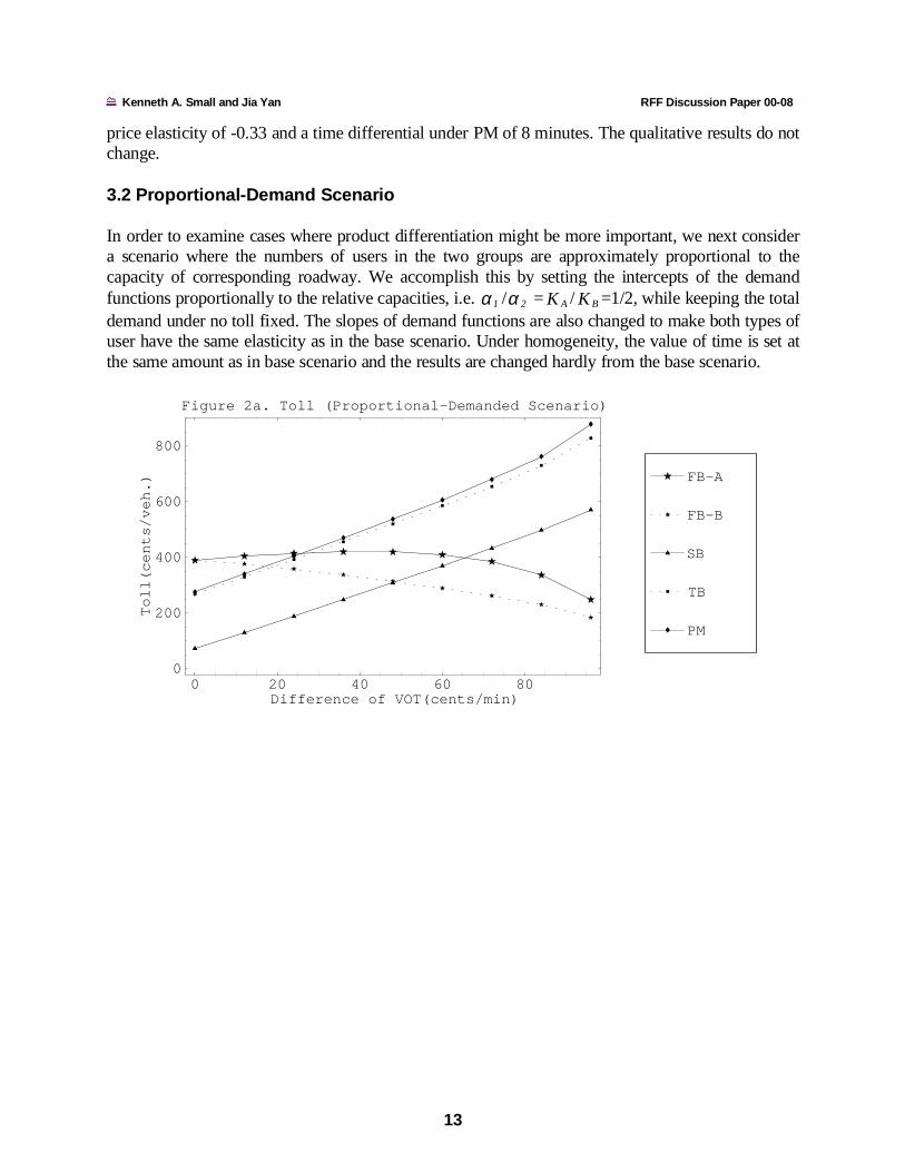
3 .2 Pro p orti o na l- De man d Sce na ri o

In order to examine cases where pr oduct di ff erenti at ion mi ght be mor e import ant , we next considera scenario wher e the numbers of user s in the two groups ar e approxim ately pr oporti onal to thecapacit y of cor respondi ng roadway. We accomplish thi s by set ting the inter cepts of the dem andfunctions pr oporti onall y t o the relative capaci ties, i. e. 1α / 2α = AK / BK =1/2, whil e keeping the totaldemand under no toll fi xed. The sl opes of demand functi ons are also changed to make bot h types ofuser have the same elasticit y as in the base scenari o. Under homogeneit y, the value of tim e is set atthe sam e amount as i n base scenari o and the result s are changed hardly from the base scenari o.

0 20 40 60 80Difference of VOT(cents/min)

0

200

400

600

800

Toll(cents/veh.)

Figure 2a. Toll (Proportional-Demanded Scenario)

PM

TB

SB

FB-B

FB-A


1 4

0 20 40 60 80Difference of VOT(cents/min.)

-25

0

25

50

75

100

125


Figure 2b. Welfare gain (Proportional-Demand Scenario)

PM

TB

SB

FB

NT

We intr oduce the het erogenei ty in this scenario by incr easing 1α twi ce as fast as we decrease 2α .Thus the distri but ion of val ues of time becomes not onl y disper sed but also skewed. The sl opes ofdemand funct ions are changed as in the base scenar io. The resul ts ar e shown in Figur e 2a-b. At thefar right of each of the panels, t he value of t ime of type 1 users i s 2.37 cent s/m in., whi le that of type2 users is 98.40 cents/ min.

Fi gure 2a shows the change of t oll s wit h value of ti me dif ference. T he pat tern of change i s sim ilar tobase scenari o. Figur e 2b shows that the welf are gain fr om fi rst -best (F B) pr ici ng is al most the sameas i n the base scenario. But this ti me the T B and PM policies are consi der ably im pr oved, gener ati ngposi tive wel far e gai ns under moder at e t o lar ge het er ogenei ty. F urt hermore, t he second-best poli cy ismuch more ef ficient in thi s scenar io, with relative eff ici ency around 45% wi th moder ate value-of-ti me di fferences. The reason for these resul ts is that the diff erent iat ed pr oduct is better mat ched tothe dif fer ent user t ypes i n thi s scenar io; f ewer users are f orced into the wrong qualit y.

The change of travel ti me under each policy in thi s scenar io is al most the same as the one in basescenari o, so is not shown.

3 .3 Hig h -Ela s ti ci ty an d Hig h- Co n ge st i on Sce n ario s

Here we fi rst consider a scenar io wi th higher price elasti ci ty of demand, namel y -0. 60 in the no- tol lregi me. The wei ghed average val ue of ti me is kept at 34.38 cent s/m in. Result s are shown in Figures3a and 3b.

Fi gure 3a shows that the second-best toll is much hi gher, and the fi rst -best lower , in thi s scenar io.This is well known from pr evious studies (Verhoef et al., 1996); wel fare- maxim izi ng policies arenow aim ed more at moder ati ng total demand than at di str ibuti ng dem and across the t wo roads.


1 5


200

300

400

500

600Toll(cents/veh.)

Figure 3a. Toll (High-Elasticity Scenario)

PM

TB

SB

FB-B

FB-A


0

50

100

150


Figure 3b. Welfare gain (High-Elasticity Scenario)

PM

TB

SB

FB

NT

Fi gure 3b shows that the eff ici ency of the PM and TB policies is improved si gni ficantly. Bot h ofthem can generate posit ive welf are gain when value of time diff erence is greater than 30 cents/ min.SB is not im proved, because it emphasizes the toll diff erent ial , whi ch is less impor tant now. Thusthe gap between SB and the other constr ained policies i s l ess, though stil l there.

Next , we consider a scenar io wi th hi gher congestion, namel y a t ravel -ti me di fferenti al of 15 mi nut esunder P M. We again accompl ish t his by changi ng the i ntercept s and sl opes of the demand funct ions.

The result s, shown in F igures 3c and 3d, are mostl y sim ilar to the base scenari o, but two di fferencesst and out. The TB policy produces a much higher toll than PM because of the heavier traffi c; andPM now all ows substanti al congesti on on the tol l lanes. The wel far e eff ect s in thi s scenar io ar esi mi lar to t hose i n the hi gh-el ast icity scenari o.


1 6


0

200

400

600

800

1000

1200Toll(cents/veh.)

Figure 3c. Toll (High-Congestion Scenario)

PM

TB

SB

FB-B

FB-A


-100

0

100

200


Figure 3d. Welfare gain (High-Congestion Scenario)

PM

TB

SB

FB

NT

3 .4 Rev e rs ed - Ca pa ci t y Sc e na ri o

In order to make a full y separated equi libri um mor e likely, we tri ed inter changing the two roadwaycapacit ies: 4000 veh/ hr for t he express lanes and 2000 for the free lanes. Al l other par ameters are asin t he base scenar io.

Results ar e shown in Fi gur e 4. The t hree one-route pricing poli cies have higher toll s in t hi s scenar iobecause the free roadway is less import ant as a substit ute. SB has a hi gher wel far e gai n because itcan charge f or mor e capaci ty. P M and TB generat e bigger welf are losses.


1 7

We get dif ferent equili bri um cases in this scenari o. Most inter est ing, as heter ogeneity is incr eased,user di fferences sim ply become too great to be wor th accom modat ing on a shar ed roadway, and theopti mal equi libria t end to become fully separat ed (S E).


0

200

400

600

800

1000

1200

Toll(cents/veh.)

Figure 4a. Toll (Reversed-Capacity Scenario)

PM

TB

SB

FB-B

FB-A


-100

-50

0

50

100


Figure 4b. Welfare gain (Reversed-Capacity Scenario)

PM

TB-SE

TB-SE2

SB-SE

SB-SE1

FB-SE

FB-SE1

NT

When the val ue of ti me dif ference is extreme large, the welf are gain fr om SB is very cl ose to that fr om FB. T he relat ive effici ency of TB pol icy t o F B pol icy at this point r eaches 77% . T he ef ficiencyof PM poli cy is al so im proved compar ed wit h base scenar io, and it can produce a posi tive wel far egain when the value of tim e dif fer ence is hi gh.


1 8

4.CONCLUSION

Our result s dem onstr ate the import ance of heter ogeneity in value of tim e for evaluat ing congest ionpoli cies that offer pri cing as an option. General ly, the exi st ence of het erogenei ty favor s suchpoli cies because product dif fer ent iation then offers a great er advantage: those wi th hi gh values ofti me reap more benef its fr om the high-priced option, while those wit h low values of tim e find it all the mor e i mport ant not to be subject ed to policies aimed at the aver age user .

Nevertheless, insi st ing that one of the pr oduct s be free imposes qui te a lar ge penal ty, except whenheterogeneit y i s ext rem e. In our base scenar io and for middl ing am ounts of heterogeneit y, a second-best one-r oute pri ci ng pol icy achi eves onl y one-fi ft h to one-half the possible wel fare gai ns of fi rst-best pr ici ng, and uses a t ol l smal ler t han even the lower of the t wo optim al ly dif ferentiated t oll s.

Even more di scouragi ng is the f inding t hat poli cies that m ai ntain nearl y congestion- free t ravel in t hepr iced roadway set the pri ce far higher , and achieve far lower benef its, than second-best pr ici ng. Inthe maj ori ty of cases, the overall benefit s from pri cing are negat ive f or these poli cies. Of course, thisdoes not account for the possibili ty that such pol icies may be the only way the lanes can be built atal l, or the onl y way they can be opened to general t raf fic.

Fr om these observati ons, we draw thr ee concl usi ons about par tial-pri cing pol ici es under hi ghlycongest ed condi tions. The fi rst two are in accord wi th studi es based on homogeneous users. First,when polit ics or other consi der ati ons dict at e that one roadway be fr ee, aggr egate costs can bereduced by lett ing the pri ced roadway become at least moderatel y congested; car pooli ng mandatesor privati zation goals may prevent this, but they do so at a heavy cost . Second, under manyconditi ons part ial pricing poli cies are inadequate substit ut es for more thor oughgoing pricingpoli cies. The thir d conclusi on is that accounti ng for heterogeneit y does improve the perform ance ofpart ial -pr icing poli cies by creati ng si gni fi cant val ue for product diff erent iat ion, especi al ly when thepr ice-el asticiti es for t ot al dem and i s high and congesti on in the absence of tol ls is extr eme.


1 9

REFERENCES

Arnott, R., A. de Palma and R. Lindsey (1992) "Route choice with heterogeneous drivers andgroup-specific congestion costs" Regional Science and Urban Economics 22 pp. 71-102.

Bradford, Richard M. (1996) "Pricing, Routing, and Incentive Compatibility in MultiserverQueues," European Journal of Operational Research 89, pp. 226-236.

Braid, Ralph M. (1996) "Peak-load pricing of a transportation route with an unpriced substitute"Journal of Urban Economics 40 pp. 179-197.

Brownstone, D., Golob, T. F. and Kazimi, C. (1999) "Modeling non-ignorable attrition andmeasurement error in panel surveys: an application to travel demand modeling," IrvineEconomics Paper 99-00-06, University of California at Irvine

Dahlgren, Joy (1998) "High occupancy vehicle lanes: not always more effective than generalpurpose lanes" Transportation Research 32A, pp. 99-114

Institute of Transportation Engineers (ITE) Task Force on High-Occupancy/Toll (HOT) Lanes (1998) "High-Occupancy/Toll (HOT) Lanes and Value Pricing: A Preliminary Assessment," Institute of Traffic Engineers (ITE) Journal (June), pp. 30-32, 38, 40.

Liu, Louie Nan, and John F. McDonald (1998) "Efficient congestion tolls in the presence ofunpriced congestion: a peak and off-peak simulation model" Journal of Urban Economics44, pp. 352-366.

______ (1999) "Economic efficiency of second-best congestion pricing schemes in urbanhighway systems" Transportation Research 33B pp. 157-188.

Shmanske, Stephen (1991) "Price discrimination and congestion" National Tax Journal 44, pp.529-532

______ (1993) "A simulation of price-discrimination tolls" Journal of Transport Economics andPolicy 27, pp. 225-235

Small, Kenneth A. (1983) "Bus Priority and Congestion Pricing on Urban Expressways." In T. E. Keeler (ed.), Research in Transportation Economics, Vol. 1, (Greenwich, Connecticut: JAI Press), pp. 27-74.

Small, Kenneth A. and José A. Gómez-Ibanez (1998) "Road Pricing for CongestionManagement: The Transition from Theory to Policy," in: Road Pricing, Traffic Congestionand the Environment: Issues of Efficiency and Social Feasibility, ed. by K.J. Button andE.T. Verhoef. Cheltenham, UK: Edward Elgar, pp. 213-246.


2 0

Sullivan, E. (1998) Evaluating the impacts of the SR 91 variable-toll express lane facility: Finalreport, report to California Department of Transportation. Dept. of Civil andEnvironmental Engineering, Cal Poly State University, San Luis Obispo, California.

Toll Roads Newsletter, 40 (June 1999). Frederick, Maryland: Toll Roads Newsletter.

Transportation Research Board (1994) Highway Capacity Manual. Special Report 209, 3rdedition. Washington: National Research Council.

Verhoef, E.T., P. Nijkamp and P. Rietveld (1996) "Second-best congestion pricing: the case ofan untolled alternative" Journal of Urban Economics 40 (3) pp. 279-302.

Verhoef, Erik T., and Kenneth A. Small (1999) "Product Differentiation on Roads: Second-BestCongestion Pricing with Heterogeneity under Public and Private Ownership," IrvineEconomics Paper 99-00-01, University of California at Irvine.

Viton, Philip A. (1995), "Private roads" Journal of Urban Economics 37, pp. 260-289.

Wardrop, J.G. (1952) "Some Theoretical Aspects of Road Traffic Research" Proceedings of theInstitute of Civil Engineers, 1(II), pp. 325-378.


2 1

APPENDIX

A. 1 Th e g en e ra l fo rm of th e no n -l in ea r pro gra mmin g pro bl e m an d the p o ss ib le s ol ut io n s.

We assume that at least some type 1 users use road A and at least some type 2 users use road B.We consider a congested traffic condition, so the toll charged under a policy regime is strictlygreater than zero. The general form of the first-best (FB) problem in this paper can therefore bewritten as:

( ) ( ) ∑∑∫∫ −+=++

i ririr

NNNN

cNdttPdttPWBABA 2211

0

2

0

1max

..ts ( ) ( ) 02111111 =−+−+≡ AAAABA NNcNNPh τ (A.1a)

( ) ( ) 02122222 =−+−+≡ BBBBBA NNcNNPh τ (A.1b)

( ) 01113 =−−⋅≡ BBB cPNh τ (A.1c)

( ) 02224 =−−⋅≡ AAA cPNh τ (A.1d) ( ) ( ) 02111111 ≤−+−+≡ BBBBBA NNcNNPg τ (A.1e)

( ) ( ) 0212222 ≤−+−+≡ AAAAB NNcNNPg τ (A.1f)

0Ng B13 ≤−≡ (A.1g)

024 ≤−≡ ANg (A.1h)

where ()⋅P and ()⋅c are the functions defined by (2) and (1). Certain constraints are added for theSB, TB, and PM policy, and the objective function is replaced by toll revenues in PM policy.Because we assume 0, 21 >BA NN . (A.1a-b) are the same as (3) of the paper; (A.1c-d) areequivalent to (5c-d); (A.1e-f) to (5a-b); and (A.1g-h) to (5e).

Suppose 4321 ,,, λλλλ are the Lagrangian multipliers for the first four equality constraint

conditions, and 21 ,γγ , 43 ,γγ are those associated with the inequality constraints. According to

the Kuhn-Tucker theorem, the necessary condition for the optimal solution( )*

2*2

*1

*1

* ,,, BABA NNNNN = , ( )*4

*3

*2

*1

* ,,, λλλλλ = , ( )*4

*3

*2

*1

* ,,, γγγγγ = are:

( ) ( ) ( ) 04

1

**4

1

*** =∇−∇−∇ ∑∑== j

jji

ii NgNhNW γλ (A.2a)

( ) 0** =Ng jjγ , 4,3,2,1=j (A.2b)

0* ≥jγ , 4,3,2,1=j (A.2c)

0≤jg , 4,3,2,1=j (A.2d)


2 2

If constraints (A.1e) and (A.1f) are binding at the same time, the tolls on both routes must beequal as shown in section 2. This is impossible for SB, TB and PM policy and our numericalresults also show that this case is never optimal for FB policy. As a result, the possible solutioncases for the programming problem are only three:

1. 0*1 =γ , 0*

2 >γ (SE1);In this case, (A.2c) 02 =⇒ g , i.e., (A.1f) must be binding. This means type 2 users areindifferent for two routes. Then (A.1e) cannot be binding, i.e., type 1 users strictly prefer road Aand, from (A.1c), 0*

1 =BN .

2. 0*1 >γ , 0*

2 =γ (SE2);

In this case, constraint (A.1e) is binding and constraint (A.1f) is not binding, and 0*2 =AN .

3. 0*1 =γ and 0*

2 =γ ;In this case, we can only say (from the argument above) that (A.1e) or (A.1f) or both must benon-binding, therefore *

1BN or *2 AN or both must be zero. Considering the following three

different solution cases: 3a. (A.1f) is binding and (A.1e) is not. *

1BN is zero in this case (SE1).

3b. (A.1e) is binding and (A.1f) is not. *2 AN is zero in this case (SE2).

3c. Both (A.1e) and (A.1f) are non-binding. *1BN and *

2 AN are both zero (SE).

In the paper, we divide the programming problem into different cases (SE, SE1, SE2) and solveeach case under each policy. The above classification shows that the solutions from these casesinclude all of the possible solutions for the whole problem.

A.2 T he de ri v at io n of op t imal t o ll s of ea ch eq ui l ib ri um in e a ch p ol i cy In this section, we show how the general problem simplifies in each policy and equilibrium type(here described as "case"). In each case, we leave the non-negative constraints (A.1g-h) areimplicit, as noted in the paper, we check each of them separately and impose it as an equality ifrequired.

A. 2.1 FB Policy Case SE. Substituting 01 =BN and 02 =AN into the welfare function, the welfare maximizingproblem can be written as:

( ) ( )∫ ∫ ⋅−⋅−+=A BN N

BBBAAA NcNNcNdttPdttPW1 2

0 0

22211121 )()(max

The objective function is strictly concave because it equals the sum of four strictly concavefunctions. Therefore, the solution must be unique. The optimal traffic ( *

2*1 , BA NN ) in this case can


2 3

be solved out from the first-order conditions. The corresponding tolls on the two routes aredetermined by (A.1a-b) and can be shown to be:

( ) AAAAAA MECNcNcP 111111 ≡′⋅=−=τ( ) BBBBBB MECNcNcP 222222 ≡′⋅=−=τ

The optimal toll on each road is equal to the difference between social and private marginal coston that road, known as "marginal external cost" MEC , just as in a single-route model.

Case SE1. Substituting 01 =BN into welfare function, we get:

( ) ( ) ( ) ( ) ( )∫ ∫+

−+⋅−+⋅−+

=A BAN NN

BBBAAAAAAAA NcNNNcNNNcNdttPdttP

W1 22

0 02222122211121

max

This objective function is also strictly concave because it equals the sum of five strictly concavefunctions. The corresponding tolls are:

( ) ( ) ( ) AAAAAAAAAAAAA cPMECNNcNNNcNcNP 2221222111111 −=≡+′++′=−=τ( ) ( ) ( ) BBBBBBBAB MECNcNNcNNP 222222222 ≡′=−+=τ

The tolls are again the differences between social and private marginal costs on each route. Thesocial cost on route A includes the users of both groups; the social cost on route B includes justthe users of group 2. We also check the corner solution of 02 =AN in the simulation study.

Case SE2: Substituting 02 =AN into the welfare function, we get:

( ) ( ) ( ) ( ) ( )BBBBBBBBAAA

NNN

NNcNNNcNNcNdttPdttP

WBBA

212221111110

20

1

211

max

+−+−−+

=

∫∫+

Again, the objective function is strictly concave so the so the solution is unique. The tolls todecentralize the optimal traffic allocation in this case are:

( ) ( ) AAAAABAA MECNcNcNNP 11111111 ≡′=−+=τ( ) ( ) ( ) BBBBBBBBBBBBAB cPMECNNcNNNcNcNNP 22212221111111 −=≡+′++′=−+=τ

Here the social cost on route A includes just the users of group 1 and the social cost on route Bincludes the users of both groups. The corner solution of 01 =BN is also checked in thesimulation study.


2 4

A. 2.2 SB and TB Policies

Case SE . The welfare maximizing problem under second-best pricing policy for fullyseparated equilibrium case can be written as:

( ) ( ) ( ) ( )∫ ∫ −−+=A BN N

BBBAAA NcNNcNdttPdttPW1 2

0 0

22211121max

..ts ( ) ( )BBB NcNP 2222 =

BN 2 is determined solely by the constraint and numerical results in the paper show that there is

only one positive real solution for BN 2 . The objective function is a strictly function of AN1 , so ifthis case can occur, the solution is unique. The corresponding toll on route A is:

( ) AAAAA MECNcN 1111 ≡′=τ

This toll is just the difference of social and private marginal cost on that road, the social costincluding just the users of group 1. There are no route spill-overs in fully separated equilibrium:that is, road A is treated just as in the FB policy.

Case SE1. The corresponding Lagrangian is:

( ) ( ) ( ) ( ) ( )

( ) ( ) ( )[ ]( ) ( )[ ]BBBA

AAAAAAA

BBBAAAAAAAA

NNN

NcNNP

NNcPNNcNP

NcNNNcNNNcNdttPdttPLBAA

222222

2122211111

22221222111

0

2

0

1

221

−+−++−+−−

−+−+−+= ∫∫+

λλ

where the constraints (A.1a-b) have been rewritten using (A.1f) as an equality in order toeliminate Aτ as a variable. The Lagrangian Multiplier 1λ represents the "Shadow Price" of notprice discriminated on road A, that is, it represents the increase of social welfare that could beachieved by charging type-1 users more than type-2 users, since the latter have a sub-optimallypriced substitute (road B).This problem can be solved for BAA NNN 221 ,, and 21,λλ . The tollwhich decentralizes the solution allocation is then determined by (A.1a) as:

( )

′′−′′−′′

′+′−′⋅′′−′+′=

BB

AABBAAAAA cPcPPP

ccPcNPcNcN

221121

2112222211τ

The toll on route A equals to marginal external cost plus an adjustment term which depends onthe slope of demand function and cost function.

Case SE2. The Lagrangian is:


2 5

( ) ( )[ ] ( ) ( )[ ]BBBBABBBB NNcNNPNNcNPWL 2111111212222 +−+−+−−= γλ

where (A.1e) has been used as an equality with Larangian multiplier 1γ which represents the"shadow price" of not being able to price discriminated on road B.

Again, we solve and use (A.1a) to determine the toll on route A as:

( )

′′−′′−′′

′′′−′−+′=

BB

BBBBAAA cPcPPP

PPcNcNcN

122121

12221111τ

The toll here equals to the marginal congestion cost plus a adjustment term which depends on theslope of demand function as well as costfunction.

It is difficult to judge analytically whether the solution is unique in case SE1 and SE2 of SBpolicy because of the non-linear form of the constraints. In the simulation study, we use differentinitial values to show that in these cases no more than one equilibrium solution can be found.

The TB policy is the same as the SB policy except that we add an extra constraint (6), which wecheck separately rather than including in the Lagrangian.

A. 2.3 PM Policy

The maximizing problem here has the same constraints as the ones in the SB policy. The onlydifferent is that the objective function now is:

( ) ( ) ( )[ ] ( ) ( )[ ]AAaBAAAAAAA NNcNNPNNNcNPNR 2122222211111 +−+++−=

Case SE . The solution of this case must be unique because the same reason as SE case in SBpolicy. The toll which maximizes revenue is found to be:

( ) ][ 1111′−′= PNcN AAAAτ

The toll is set at marginal social cost plus a monopolistic mark-up which is inversely related tothe demand elasticity of group 1. Equivalently, this equation can be written as

AAAA cNPN 1111 ′=′+τ , that is, marginal revenue equals marginal cost.

Case SE1. The toll is found to be:

( )

′′+′−′′−′′

′+′−′′′−′′+′′+′−′+′=

BB

AABAABAAAAAAA cPPcPPP

ccPcPNPPNcPNPNcNcN

222

22121

211211211222112211 )(2

)(τ

Again the toll equals marginal congestion cost plus a monopolistic mark-up.


2 6

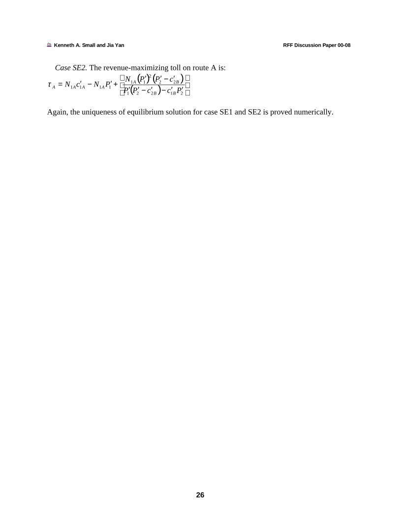
Case SE2. The revenue-maximizing toll on route A is:

( ) ( )( )

′′−′−′′

′−′′+′−′=

21221

222

111111 PccPP

cPPNPNcN

BB

BAAAAAτ

Again, the uniqueness of equilibrium solution for case SE1 and SE2 is proved numerically.

Documents

The Value of 'Value Pricing' of Roads: Second-Best … · Second-Best Pricing and Product Differentiation Kenneth A. Small Jia Yan Discussion Paper 00-08 ... be far lower than the