The value of the trout fishery at Rhodes, North Eastern Cape, South Africa:

A travel cost analysis using count data models

M Du Preez & S G Hosking

Working Paper Number 182

The value of the trout fishery at Rhodes, North EasternCape, South Africa: A travel cost analysis using count data

models

M Du Preez∗& S G Hosking †

July 1, 2010

Abstract

The National Environmental Management: Biodiversity Act, no.10 of 2004) makes provisionfor the presence of alien trout in South African waters by means of a zoning system, partly inrecognition of the significant income generating potential of trout fishing in South Africa. Thispaper reports the first formal recreational valuation of a trout fishery in South Africa, the onein and around Rhodes village, North Eastern Cape. The valuation is carried out by applyingthe individual travel cost method using several count data models. The zero truncated negativebinomial model yielded the most appealing results. It accounts for the non-negative integer natureof the trip data, for truncation and over-dispersion. The paper finds that in 2007 consumersurplus per day visit to the Rhodes trout fishery was R2 668, consumer surplus per trip visit wasR13 072, and the total consumer surplus generated was R18 026 288.

1 IntroductionThe merit of the presence of Rainbow and Brown trout in South African waters has been challengedin recent years by increased negative publicity toward alien plants and animals (Bainbridge et al.,2008). In total twenty-four alien fish species, equivalent to 9 % of all South African freshwaterfish species, were introduced into and established in South African waters during the 19th and 20th

Centuries (Skelton, 2001). Of the twenty-four introduced species, trout have become South Africa’smost widely spread and used freshwater fish species — mainly because they are in such high demandas a target for recreational fishing (Bainbridge et al., 2005). The trout fishing industry has alreadybeen shown to be a source of income, as well as a job creator, in some of the poorest, most rural partsof South Africa (Bainbridge et al., 2005; Hlatswako, 2000; Rogerson, 2002). The industry provides atwo-tier service: first, in food production and second, as a recreational angling resource. Recreationalangling, including fly-fishing for trout, is a major tourism attraction in South Africa (Bainbridge etal., 2005). The trout fishing industry is sustained and underpinned by a considerable service industryconsisting of tackle manufacturers and retailers, tourist operators, professional guides, hotels, lodgesand bed and breakfast establishments. The trout is also viewed as an indicator of good water qualityin South African streams and rivers.The National Environmental Management: Biodiversity Act, no. 10 of 2004 (NEMBA) explicitly

recognizes the value of trout and makes provision for their management. Both trout species have beenlisted in Category 4 of the NEMBA Alien Regulations for alien animals and plants, to be managedby way of a zoning system (Impson, 2008). Within the zones trout fishing will be promoted but

∗Department of Economics, Tourism and Development Studies, Nelson Mandela Metropolitan University†Department of Economics, Toursim and Development Studies, Nelson Mandela Metropolitan University

1

outside the zones, however, trout fishing and farming will be controlled (Impson, 2008). “. . . everyeffort will be made to protect premier trout waters in South Africa. Everyone is aware that thesewaters are economically valuable and cherished by a substantial number of South Africans” (Impson,2008).One of these premier trout waters is the Rhodes fishery situated in the North Eastern Cape,

South Africa. The rivers and streams that make up the Rhodes fishery are easily accessible andmainly inhabited by a self-sustaining population of wild trout (both Rainbow and Brown). If onewere to eradicate the trout in this region (because it is an alien species) there would be substantialcosts incurred. The most feasible way would be poisoning — but even this would be very costly —direct costs plus those of eradicating other species and foregone recreational value.How big would the opportunity cost be? This study is the first formal attempt to value this cost

- the recreational trout fishery in South Africa. A specific trout fishery was selected for this purpose- the one in and around Rhodes village, North Eastern Cape1.The method adopted in this paper to value the trout fishing benefit is the individual travel cost

method. This method is well suited to valuing the benefits of a trout fishery because travel cost isoften the main expenditure incurred by a cross-section of fly-fishers (Loomis & Walsh, 1997). Dueto the count, truncated and over-dispersed nature of the data count data models were estimated inthis study.

2 The travel cost methodMany travel cost studies have been conducted in the United States and elsewhere to value recreationalsites (Caulkins et al., 1986; Kling, 1987; Liston-Heyes & Heyes, 1999; Bowker et al., 1996; Fix &Loomis, 1997; Bin et al., 2005; Martinez-Espineira & Amoako-Tuffour, 2008). Examples of theapplication of the method to value recreational fisheries include Morey et al. (1993), Layman etal. (1996), Gillig et al. (2000), Curtis (2002) and Shrestha et al. (2002). Morey et al. (1993) andCurtis (2002) employed the travel cost method to estimate the value of Atlantic salmon recreationalfisheries — one in the United States and the other in Ireland. The consumer surplus per day trip wasestimated as US$179 and IRPound139, respectively for the Morey et al. (1993) and Curtis (2002)studies. The travel cost method was also used to estimate values for recreational fisheries locatedin Alaska, the Gulf of Mexico and the Brazilian Pantanal (Layman et al., 1996; Gillig et al., 2000;Shrestha et al., 2002). The consumer surplus of a single day trip to the Red Snapper fishery inthe Gulf of Mexico was estimated at US$213 (Gillig et al., 2000), whereas the consumer surplusof a single day trip to Brazilian Pantanal recreational fishery was estimated at US$86 (Shrestha etal., 2002). Layman et al. (1996) estimated the consumer surplus per trip to the Alaskan salmonrecreational fishery to be US$51.Travel cost models can be broken up into single-site and multiple-site ones. The latter include

Random Utility Models (RUMs), whereas the former include the individual and zonal (Clawson-Knetsch) methods (Bockstael, 1995; Freeman, 2003). A single-site individual travel cost method(TCM) was applied in this study to estimate the total economic value of the Rhodes trout fishery.To perform the individual TCM analysis, a trip generating function (TGF) is estimated using

survey data in which travel costs predict the number of visits that will be undertaken by an individualto a recreational fishing site ( Bockstael, 1995; Pagiola et al., 2004; Ward & Beal, 2000). The travelcost incurred in undertaking the fishing trip to the site is therefore used as a proxy for the “price”paid by the visitor for the site’s use (Liston-Heyes & Heyes, 1999). Over and above travel costs, arange of explanatory variables (such as income, age, gender, educational attainment, substitute sitesand recreation site quality) are also usually included in the TGF (Bockstael, 1995; Hanley & Spash,

1Other applications of the valuation to trout fisheries include: assistance in fishery management decisions, suchas awarding zoning rights for trout fisheries in upper catchments, and determining the benefits associated with waterquality improvement projects (McConnell and Strand, 1994).

2

1993). Once the TGF is estimated, a demand function can be derived which is used to estimatethe consumer surplus or non-market value of recreational fishing (Bateman, 1993; Hanley & Spash,1993).Due to the zero truncated and non-negative integer nature of the trip data as well as the preva-

lence of over-dispersion issues, the estimation of the TGF by means of the ordinary least squares(OLS) method may lead to biased estimators (Creel & Loomis, 1990; Hellerstein & Mendelsohn,1993). As a result of these difficulties with the OLS model, the use of count data models, such as thePoisson and Negative Binomial models, have become popular (Creel & Loomis, 1991; Hellerstein,1991; Bowker et al., 1996; Englin et al., 2003). The standard Poisson model assumes a discreteprobability density function and non-negative integers (Hellerstein & Mendelsohn, 1993; Shresthaet al., 2002).The truncation problem is common in modelling recreational demand because of on-site sam-

pling. Non-visitors’ demand and the value they attach to the recreational site in question are notcaptured and therefore is excluded (Bin et al., 2005; Englin & Shonkwiler, 1995). The endogenousstratification problem is the increased likelihood that more frequent than less frequent visitors willbe captured during the administration of the surveys biasing the sample toward this group (Shaw,1988; Creel & Loomis, 1990).The recommended procedure to correct for both endogenous stratification and truncation is to

weight each observation by the expected value of visits (Shaw, 1988). When the standard Poissonmodel is applied, this correction procedure entails modifying the dependent variable by subtracting1 from each of its values (Shaw, 1988; Fix & Loomis, 1997; Hesseln et al., 2003; Hagerty & Moeltner,2005).A drawback of the Poisson model is that it assumes that the first two moments (variance and

conditional mean) of its distribution are equal. In many instances the conditional mean and thevariance are unequal - the variance exceeds the conditional mean causing over-dispersion (Cameron& Trivedi, 1990).Use of the negative binomial model is a popular way of addressing the over-dispersion problem

(Shrestha et al., 2002; Bin et al., 2005; Martinez-Espineira & Amoako-Tuffour, 2008). The unob-served heterogeneity that is not captured by the Poisson model is reflected in the negative binomialmodel by the addition of an extra parameter, α (Martinez-Espineira & Amoako-Tuffour, 2008). Inorder to test for no over-dispersion, a likelihood ratio test based on the parameter α can be admin-istered. The negative binomial model can also be adapted to correct for truncation; yielding a zerotruncated negative binomial model (Bowker et al., 1996; Liston — Heyes & Heyes, 1999; Zawacki etal., 2000; Martinez-Espineira & Amoako-Tuffour, 2008).

3 Applying the TCM to value trout fishingThe TCM is a highly appropriate method by which to value recreational assets such as trout fishingwaters because the main way demand is revealed is through travel to access these waters. Thespecific waters valued are those in and around Rhodes village, located at the foot of the southernDrakensberg Mountains in the North-Eastern Cape (See Fig. 1 below).Commercial activities in the Rhodes region comprise of farming and tourism-related businesses.

The latter include accommodation provision (for example, lodges and guesthouses), tourist guideservices and art products. One of the main tourist attractions located in and around Rhodes villageare the many rivers and streams which harbour an abundance of self sustaining populations of wildtrout (both Rainbow and Brown) (Wild Trout Association, 2008). The streams and rivers originate2800 to 3300 metres above sea level as unspoiled, rock-based highland streams. The Wild TroutAssociation (WTA) manages the rivers and streams on behalf of riparian landowners (Wild TroutAssociation, 2008). Visiting fly-fishers pay a R100 fee per day to fish in the WTA’s waters. Theriparian landowners receive R60 of each R100 paid by fly-fishers, while the WTA retains the balance

3

(Wild Trout Association, 2008). The permit allows access to more than 200 kilometres of runningwater. The fishing season in the Rhodes region runs from September to March of every year (SenquTourism, 2008).The trip data required to apply the individual travel cost method in this study was obtained by

conducting on-site personal interviews with the aid of a structured questionnaire between September2006 and September 2007. The target population comprised of all the users of trout and trout fly-fishing services provided by the rivers and streams managed by the WTA. The sampling frame wasdefined in terms of fly-fishers who purchase day permits from the WTA in order to gain access tothe rivers and streams. By averaging total annual visits (based on individual day permit sales) toWTA-rivers and streams from 2002 to 2006 it was estimated that 700 fly-fishers visit Rhodes perannum. Every seventh adult respondent purchasing a day permit from the one and only WTA daypermit vendor in Rhodes was selected. A sample of 13% of the estimated fisher population wastargeted, viz. 96 fishers.The interviewer was instructed to conduct the interviews with individuals only so as prevent the

influence of others if it was a group visit. In cases where families were encountered, the interviewerwas requested to interview the household head only.In the survey visitors were asked questions about the their home location, the round trip distance

travelled, the duration (in hours) of the round trip, the type and engine capacity of the motorvehicle used to undertake the trip, duration of the visit, the total number of trout caught duringvisits undertaken to the site during the previous year, the time taken to travel to their favouritesubstitute trout fishing site, other sites and attractions visited during the trip and some socio-economic information.No thorough examination of the characteristics of the fly-fishers who visit the Rhodes trout

fishery has ever been conducted. For this reason, it was difficult to determine whether this sample isrepresentative of the typical population of visitors to Rhodes. The only data available for comparisonpurposes was that of visitor origin for the period 2002 to August 2006 — see Table 1 (Wild TroutAssociation, 2008).The records of the population and those of the sample show similar characteristics.The TGF used predicted visit frequency on the basis of a mixture of trip characteristics such as

travel costs, travel time, socio-economic variables (income, gender, age, and race), a substitute sitevariable and an environmental quality variable and was specified as follows:

Vij = f (TC ij ,TT ij , SE ij , Sij , Eij); i = 1 . . .n (1)

where Vij is the number of trips undertaken tothe site per annum, TC ij is the travel cost incurredin visiting site j, TT ij represents the round trip travel time, SE i represents various socio-economiccharacteristics of the respondent, Sij represents information on substitute sites, Eij represents in-formation on environmental quality and n is the number of visitors .The dependent variable in this study is the number of trips undertaken to Rhodes by the indi-

vidual in the past year. It was hypothesized that travel cost, travel time, gender, race, catch rate,age, income and substitute sites would explain the number of fishing trips undertaken to Rhodes.The travel costs for each respondent were the sum of distance costs and accommodation costs.

The latter was taken to be the reported cost per night of staying in Rhodes. The distance costswere calculated by the researchers from motor vehicle operating costs. Some studies use reportedtravel (distance) costs (Fix and Loomis, 1998) while other studies use researcher-calculated travelcosts (Martinez-Espineira and Amoako-Tuffour, 2008). Bowker et al. (1996) found no significantdissimilarities between the methods, Common et al. (1999) found that ‘researcher assigned costs’ are33 percent above respondent perceived costs and Hagerty and Moeltner (2005) found that travellersbehave in a way that suggest that their individual travel costs per mile are less than those basedon engineering considerations. The latter suggests that individuals are either ignorant of true travelcosts, or that there exists unaccounted for factors related to driving which have a ‘cost-decreasingeffect’ (Hagerty and Moeltner, 2005). The calculation of the travel costs by the researchers in this

4

study was done in an attempt to prevent respondent fatique, and recollection and response bias(Martinez-Espineira & Amoako-Tuffour, 2008).Following standard practice in the literature (Hesseln et al., 2003; Bin et al., 2005; Martinez-

Espineira & Amoako-Tuffour, 2008), the total operating costs per kilometre were multiplied by theroundtrip distance (to and from Rhodes) travelled. Total operating costs were estimated by summingthe fixed costs and running costs of operating a motor vehicle, as provided by the AutomobileAssociation of South Africa (AA). The fixed costs include the cost of licensing, depreciation andinsurance. To compute the running costs of a motor vehicle, the AA uses the engine capacity, theannual maintenance costs and the fuel costs per kilometre.The inclusion of time costs in travel cost studies has been subject to much debate (Freeman,

2003; Zawacki et al., 2000; Hesseln et al., 2003; Parsons, 2003; McKean et al., 2003). Some studiessuggest that some fraction of the wage rate be used to estimate the opportunity cost of time (Cesario& Knetsch, 1970; Cesario, 1976; Bateman, 1993; Bowker et al., 1996; Liston-Heyes & Heyes, 1999;Zawacki et al., 2000; Hagerty & Moeltner, 2005; Martinez-Espineira & Amoako-Tuffour, 2008).Travel time costs ranging between 25% and 50% of the wage rate are commonly thought to beappropriate (Bateman, 1993; Bowker et al., 1996; Zawacki et al., 2000), particularly 30% (Sarker& Surry, 1998; Liston-Heyes & Heyes, 1999; Sohngen et al., 2000; Hagerty & Moeltner, 2005;Martinez-Espineira & Amoako-Tuffour, 2008). Normally, the time cost of travelling is calculatedas the product of the number of hours travelled and the opportunity cost of time per hour (thehourly wage rate multiplied by a fixed fraction). Some studies calculate the hourly wage rate foreach individual by dividing their annual income by total number of working hours per annum (Binet al., 2005; Martinez-Espineira & Amoako-Tuffour, 2008). Other studies choose to omit travel timecosts completely (Hanley et al., 2003). In this study, the round trip travel time variable is treatedseparately, so permitting the calculation of the opportunity cost of travel time endogenously (Loomis& Walsh, 1997; Shrestha et al., 2002).The following socio-economic variables were also included, gender, race, age, and income. Many

travel cost studies have found income to have a negative or non-significant influence (Liston-Heyes& Heyes, 1999; Sohngen et al., 2000; Loomis, 2003). Others have found income to have a positiveand significant influence (Bin et al., 2005; Martinez-Espineira & Amoako-Tuffour, 2008). Being veryremote makes the visit and fishing at Rhodes village expensive enough for many fly-fishers. Forthis reason it was expected that income would have a positive influence (recreational fishing beinga normal good) on the number of fishing trips undertaken per annum.The TGF should, ideally, also include a substitute site variable because two visitors who travel

an equivalent distance to visit a recreation site may value it entirely differently. The differences invaluation of a site by the two visitors may be because one visitor has a substitute site available whilethe other does not (Bateman, 1993; Hanley & Spash, 1993; Perman et al., 1996). This influence canbe incorporated by including distance to a substitute site as a variable or a dummy variable thatassumes a value equal to one if the individual suggested a substitute site was considered or zeroif not (Bowker et al., 1996; Martinez-Espineira & Amoako-Tuffour, 2008). Many studies omit theprice of substitutes (Creel & Loomis, 1990; Liston-Heyes & Heyes, 1999). Smith and Kaoru (1990)have argued that the omission of substitutes leads to an over-estimation of consumer surplus. Inthis study, the influence of substitute sites on visitation rates is reflected by the person’s roundtriptravel time (measured in hours) to his or her most favoured alternative (substitute) site.The environmental quality variable included in the TGF depends on the type of recreation site

being valued. Examples of environmental quality indicators are the level of pollution, the availabilityand quality of infrastructure at the site, temperature, and the amount of congestion at the site. Inrecreational fishing studies, the catch rate variable is a common environmental quality indicator(McConnell & Strand, 1994). It was also used in this study. Table 2 provides the operationaldefinitions and a priori expectations of the variables used in constructing the recreational demandmodel of trout fly-fishing.The descriptive statistics of the variables used in the regression analysis are shown in Table 3.

5

The majority (98%) of the fly-fishers interviewed were white males. Respondent age rangedbetween 19 and 69 years, with a mean age of 41 years. The survey also revealed that 16% ofrespondents earn in excess of R1 million per annum compared to only 6% who earn R120 000 or lessper annum. The average income was R848 020 per annum. On average, visitors caught a total of35 trout during trips undertaken in the previous year.

4 The multi-purpose trip problemThe issue of multi-purpose trips is a problem that is unique to the application of the TCM (Bateman,1993; Freeman, 2003; Martinez-Espineira & Amoako-Tuffour, 2008). Normally, a custom is followedwhereby “meanderers” are distinguished from “purposeful visitors” (Hanley & Spash, 1993). Theformer are those people for whom a recreational site visit is only part of the reason for their journey.The latter are those people for whom a recreational site visit is the only reason for their trip. Itis very difficult to allocate a proportion of travel costs to meanderers (Hanley & Spash, 1993). Ithas been shown by Martinez-Espineira & Amoako-Tuffour (2008) that ignoring the multi-purposenature of trips leads to an over-estimation of consumer surplus by almost 50%. The problem of multi-purpose trips is also encountered in fly-fishing visits. In order to deal with this issue, respondentswere asked to score the importance of fly-fishing for trout, among other activities, relative to theimportance they attach to the entire trip. The score, expressed as a percentage, was then used toweight their aggregate travel cost. Weighting the aggregate travel cost per fisher resulted in thefollowing transformation:

WTC = ATC ∗ w (2)

where WTC is the weighted aggregate travel cost per fisher, ATC is the unweighted aggregate travelcost per fisher, and w is the weighting factor expressed as the percentage time spent fly-fishing fortrout. The majority of the respondents, namely 89%, stated that the sole reason (a 100% score) fortheir trip was to fly-fish for trout in the Rhodes fishery.

5 Results and discussionFour types of econometric specifications were used in this study to estimate a recreational fishingtrip demand model, namely a standard Poisson specification, a Poisson specification adjusted fortruncation and endogenous stratification (ES Poisson), a standard negative binomial specification(NB), and a zero truncated negative binomial specification (ZTNB).The same covariates were used in each of the abovementioned estimations. In addition, separate

slope parameters were estimated for the different specifications, because the estimated coefficientsof the Poisson and negative binomial models can not be interpreted as marginal effects. The resultsof applying various count data models in Stata: Release 10.1 are shown in Table 4 below.The different models of recreational demand presented in Table 4 above are robust — there are

no coefficient sign changes across models, the magnitudes of the coefficients are very similar, andonly the statistical significance and the goodness of fit measures are slightly dissimilar. According toTable 4, the Poisson model (ES Poisson) adjusted for zero truncation and endogenous stratificationbest fits the data (the Pseudo R2 = 0.1246 and six of the eight explanatory variables are statisticallysignificant).Over-dispersion is a problem since the over-dispersion parameter α in both the negative bino-

mial (NB) and the zero truncated negative binomial (ZTNB) models is highly significant. Morespecifically, a likelihood-ratio test of α equal to zero based on the NB results in a χ2 (01) = 80.92with Prob>= χ2 = 0.000, while a likelihood-ratio test of α equal to zero based on the ZTNB resultsin a χ2 (01) = 83.81 with Prob>= χ2 = 0.000. Both the recreational demand models based on

6

the Poisson distribution, namely Poisson and ES Poisson, are overly restrictive because they donot take into account that a small number of fishers undertake many trips while a large number offishers undertake only a few trips — a problem that is averted by the use of the negative binomialmodel. Although both negative binomial models account for the count nature of the data and over-dispersion, the ZTNB model is preferred over the NB model, since the former also accounts for zerotruncation. Moreover, both the log-likelihood function value and the information measures (AICand BIC) suggest that the ZTNB model performs better than the NB model. The discussion belowrelates to the preferred ZTNB model.Estimates of the ZTNB model show that the estimated coefficient for the travel cost variable is

negative and significant (Table 4). The negative sign of this variable’s coefficient suggest a downward-sloping demand curve — fishers undertake fewer trips as travel costs rise. This result is stronglyreinforced by the coefficient of the travel time variable — it has a negative sign and is statisticallysignificant at the 10% level. The marginal effects of the travel cost and travel time variables can beused to estimate the opportunity cost of travel time. An increase of R1757.78 in travel cost entailsa one-trip decrease in visitation (calculated from Table 4). A decrease of one trip entails an increaseof 8.40 hours in travel time. Therefore, an hour of travel time costs R209.26 in recreational fishing.Coincidently, the magnitude of this travel time estimate is similar to the estimate calculated byShrestha et al. (2002) for recreational fishing in the Brazilian Pantanal, namely $23.43 per hour.The coefficients of the gender, age, race and income variables were insignificant. As expected the

catch rate variable has a positive coefficient and is significant at the 1% level. Fishers who catchmore fish per trip are likely to undertake more frequent trips to Rhodes. The sign of the coefficientof the substitute site variable accords with a priori expectations. It is positive and statisticallysignificant at the 10% level. This result suggests that those fishers with higher round trip traveltimes to substitute sites undertake more visits to Rhodes, ceteris paribus.

6 Welfare calculationsFor the purposes of comparison, welfare estimates were obtained using all four models. The welfaremeasures calculated in this study apply only to the relevant user population. The recreationaldemand model, adjusted for zero truncation, count data and over-dispersion, could not be applied toextrapolate welfare measures to non-users because of several reasons. First, the non-user populationcould not be identified and defined in this study. Second, it was unclear whether non-users have thesame demand functions as users (Hellerstein, 1991; Martinez-Espineira & Amoako-Tuffour, 2008).Finally, population values for the parameters in the demand equations were unobtainable (Englin &Shonkwiler, 1995; Martinez-Espineira & Amoako-Tuffour, 2008).The estimated coefficients of the travel cost covariate for each count data model were used to

calculate the welfare measures (see Table 5 below). The average consumer surplus per visit estimateswere calculated as the negative inverse of the travel cost coefficient (-1/β̂) (Creel & Loomis, 1990).This particular method of calculating consumer surplus per visit estimates is possible because acount data model is used (Loomis et al., 2001). Table 5 below presents the estimation results of thewelfare measures at the mean of the data. The consumer surplus per angler per trip was calculatedto be R13 072 using the regression results of the preferred zero truncated negative binomial model.Per day consumer surplus estimates were obtained by using the mean length of the visit in days

and equals R2 668. The total consumer surplus figures of trout fishing in Rhodes were obtainedusing the predicted total annual trips by the fisher population. Based on a fisher population of700, and taking the predicted number of trips per fisher per annum, the aggregate annual numberof trips was estimated. The preferred ZTNB model yields a lower estimate of aggregate consumersurplus per annum, namely R18 026 288, compared to the two Poisson models estimated, but yieldsa slightly higher estimate compared to the standard negative binomial model.

7

7 ConclusionThe law of South Africa makes provision for maintaining trout habitats. There is good reason forthis law — trout fishing makes a significant economic contribution in many regions of South Africa;the North Eastern Cape being one. The trout are legally here and would cost a lot to remove.In addition, there would be WTP foregone as a result of such removal. This paper estimates theforegone recreational value cost as being the order of R18 million. The valuation method employedwas the travel cost one. While the welfare estimates calculated in this study are conditional uponthe survey sample, they do show the substantial benefit of the trout resource. This benefit value isimportant from a resource policy point of view. Monetary estimates of the Rhodes trout fishery canassist in fishery management decisions, such as awarding zoning rights for this trout fishery in uppercatchments. These estimates can also be of use in comprehending the benefits associated with waterquality improvement projects in this area (McConnell and Strand, 1994).In addition to the recreational value foregone there are also some trickle down benefits to the

poor that result from the trout fishing industry in the Rhodes area. Money is injected into theregion through the purchase of rights to fish and provision of accommodation and other services.This income, in turn, is used to employ staff to provide the relevant services. This paper did notestimate the proportion of this income reaching the poor, but given the limited scope for economicactivity in this region, we think that it has a meaningful beneficial impact.

8 Notes1. The costs associated with the negative biodiversity impacts of trout have to date not beenestimated in South Africa.

References[1] Automobile Association of South Africa (2008) AA Rates for Vehicle Operating Costs, Available

from: http://www.AA.co.za/vehicle operating cost (Accessed: 2 June 2008).

[2] Bainbridge, W., Alletson, D., Davies, M., Lax, I. & Mills, J. (2005) The Policy of FOSAF onthe Presence of Trout in the Freshwater Aquatic Systems of South Africa and Southern Africa.(Johannesburg, Federation of Southern African Fly-fishers).

[3] Bateman, I.J. (1993) Valuation of the environment, methods and techniques: revealed prefer-ence methods, in: R. K. Turner (Ed.) Sustainable Environmental Economics and Management(London, Belhaven Press).

[4] Bin, O., Landry, C.E., Ellis, C. & Vogelsong, H. (2005) Some consumer surplus estimates forNorth Carolina beaches, Marine Resource Economics, 20(2), pp. 145 — 161.

[5] Bockstael, N., McConnell, K. & Strand, I. (1991) Recreation, in: J. Braden & C. Kolstad (Eds.)Measuring the Demand for Environmental Quality (Amsterdam, Elsevier).

[6] Bockstael, N.E. (1995) Travel cost methods, in: D. W. Bromley (Ed.) The Handbook of Envi-ronmental Economics (Oxford, Blackwell).

[7] Bowker, J.M., English, D.B.K. & Donovan, J.A. (1996) Toward a value for guided rafting onsouthern rivers, Journal of Agricultural and Applied Economics, 28(2), pp. 423 - 432.

[8] Boyle, K.J., Roach, B. & Waddington, D.G. (1998) 1996 Net Economic Values for Bass, Troutand Walleye Fishing, Deer, Elk and Moose Hunting, and Wildlife Watching (Washington DC,Prepared for U.S. Fish and Wildlife Service).

8

[9] Cameron, A.C. & Trivedi, P.K. (1990) Regression-based tests for overdispersion in the Poissonmodel, Journal of Econometrics, 46(3), pp. 347 — 364.

[10] Caulkins, P.P., Bishop, R.C. & Bouwes, N.W. (1986) The travel cost model for lake recreation:a comparison of two methods for incorporating site quality and substitution effects, AmericanJournal of Agricultural Economics, 68, pp. 291 — 297.

[11] Cesario, F.J. & Knetsch, J.L. (1970) Time bias in recreation benefit estimates,Water ResourcesResearch, 6(3), pp. 700 -704.

[12] Cesario, F. (1976) Value of time in recreation benefit studies, Land economics, 52, pp. 32 — 41.

[13] Common, M., Bull, T. & Stoeckl, N. (1999) The travel cost method: an empirical investigationof Randall’s difficulty, Australian Journal of Agricultural and Resource Economics, 43(4), pp.457 — 477.

[14] Creel, M. & Loomis, J.B. (1990) Theoretical and empirical advantages of truncated countdata estimators for analysis of deer hunting in California, American Journal of AgriculturalEconomics, 72, pp. 434 — 441.

[15] Creel, M. & Loomis, J.B. (1991) Confidence intervals for welfare measures with application toa problem of truncated counts, The Review of Economics and Statistics, 73(2), pp. 370 — 373.

[16] Curtis, J.A. (2002). Estimating the demand for salmon angling in Ireland, The Economic andSocial Review, 33(3), pp. 319 — 332.

[17] Englin, J. & Shonkwiler, J. (1995) Estimating social welfare using count data models: Anapplication under conditions of endogenous stratification and truncation, Review of Economicsand Statistics, 77, pp. 104 — 112.

[18] Englin, J.E., Holmes, T.P. & Sills, E.O. (2003) Estimating forest recreation demand using countdata models, in: E.O. Sills (Ed.) Forests in a Market Economy (Dordrecht, Kluwer AcademicPublishers).

[19] Fedler, A.J. (1987) Trout Fishing in Maryland, An Examination of Angler Characteristics,Behaviors and Economic Values (Annapolis, Maryland Department of Natural Resources).

[20] Fix, O. & Loomis, J. (1997) The economic benefits of mountain biking at one of its meccas:An application of the travel cost method to mountain biking in Moab, Utah, Journal of LeisureResearch, 29(3), pp. 342 — 352.

[21] Fix, O. & Loomis, J. (1998) Comparing the economic value of mountain biking estimated usingrevealed and stated preference, Journal of Environmental Planning and Manangement, 41(2),pp. 227 — 236.

[22] Freeman, A.M. (2003) The Measurement of Environmental and Resource Values: Theories andMethods (Washington DC, Resources of the Future).

[23] Gillig, D., Ozuna, T. & Griffin, W.L. (2000). The value of the Gulf of Mexico recreational RedSnapper fishery, Marine Resources Economics, 15(2), pp. 127 — 139.

[24] Hagerty, D. & Moeltner, K. (2005) Specification of driving costs in models of recreation demand,Land Economics, 81(1), pp. 127 — 143.

[25] Hanley, N. & Spash, C. (1993) Cost-benefit Analysis and the Environment (Vermont, EdwardElgar).

9

[26] Hanley, N., Bell, D. & Alvarez-Farizo, B. (2003) Valuing the benefits of coastal water qualityimprovements using contingent and real behaviour, Environmental and Resource Economics,24(3), pp. 273 — 285.

[27] Hellerstein, D.M. (1991) Using count data models in travel cost analysis with aggregate data,American Journal of Agricultural Economics, 73, pp. 860 — 866.

[28] Hellerstein, D. & Mendelsohn, R. (1993) A theoretical foundation for count data models, Amer-ican Journal of Agricultural Economics, 75(3), pp. 604 — 611.

[29] Hesseln, H., Loomis, J.B., Gonsalez-Caban, A. & Alexander, S. (2003) Wildfire effects on hikingand biking demand in New Mexico: A travel cost study, Journal of Environmental Management,69(4), pp. 359 — 368.

[30] Hlatswako, S. (2000) Fly-fishing and Tourism: A Sustainable Rural Community Developmentfor Nsikeni (Pietermaritzburg, Unpublished Masters Dissertation, University of Natal).

[31] Impson, D. (2008) Is there a place for trout in the new South Africa? Yes! Flyfishing Magazine,21(110), pp. 26 — 28.

[32] Kling, C.L. (1987) A simulation approach to comparing multiple site recreation demand modelsusing Chesapeake Bay survey data, Marine Resources Economics, 4, pp. 95 — 109.

[33] Layman, R.C., Boyce, J.R. & Criddle, K.R. (1996) Economic valuation of the Chinook salmonsport fishery of the Gulkana River, Alaska, under current and alternate management plans,Land Economics, 72(1), pp. 113 — 128.

[34] Liston — Heyes, C. & Heyes, A. (1999) Recreational benefits from the Dartmoor National Park,Journal of Environmental Management, 55(2), pp. 69 — 80.

[35] Loomis, J.B. & Walsh, R.G. (1997) Recreation Economic Decisions: Comparing Benefits andCosts (2nd ed.) (State College, PA, Venture Publishing, Inc).

[36] Loomis, J.B., Rosenberger, R. & Shrestha, R.K. (1999) Updated Estimates of Recreation Valuesfor the RPA Program by Assessment Region and Use of Meta-Analysis for Recreation BenefitTransfer (Fort Collins, Colorado State University, Final Report for the USDA Forest Service).

[37] Loomis, J.B., Gonzalez-Caban, A. & Englin, J. (2001). Testing for differential effects of forestfires on hiking and mountain biking demand and benefits. Journal of Agricultural and ResourceEconomics, 26(2), pp. 508 -522.

[38] Loomis, J. (2003) Travel cost demand model based river recreation benefit estimates with on-site and household surveys: Comparative results and a correction procedure, Water ResourcesResearch, 39(4), pp. 1105.

[39] Markowski, M., Unsworth, R., Paterson, R. & Boyle, K. (1997) A Database of Sport FishingValues (Washington DC, Industrial Economic Inc. prepared for the Economics Division, U.S.Fish and Wildlife Service).

[40] Martinez-Espineira, R. & Amoako-Tuffour, J. (2008) Recreation demand analysis under trun-cation, overdispersion, and endogenous stratification: An application to Gros Morne NationalPark, Journal of Environmental Management, 88(4), pp. 1320 — 1332.

[41] Martinez-Espineira, R. & Amoako-Tuffour, J. (2008) Multi-destination and Multi-purpose TripEffects in the Analysis of the Demand for Trips to a Remote Recreational Site (Brussels, Eco-nomics and Econometrics Research Institute EERI Research Paper Series No. 19/2008).

10

[42] McConnell, K.E. & Strand, I.E. (1994) The Economic Value of Mid and South Atlantic Sport-fishing, Volume 2 (College Park, University of Maryland).

[43] McKean, J.R., Johnson, D. & Taylor, R.G. (2003) Measuring demand for flat water recreationusing a Two-Stage/Disequilibrium travel cost model with adjustment for overdispersion andself-selection, Water Resources Research, 39(4), pp. 1107.

[44] Morey, E.R., Rowe, R.D. & Watson, M. (1993) A repeated nested logit model of Atlantic salmonfishing, American Journal of Agricultural Economics, 75(3), pp. 578 — 592.

[45] Pagiola, S., Ritter, K. & Bishop, J. (2004) Assessing the Economic Value of Ecosystems (Wash-ington DC, World Bank).

[46] Parsons, G.R. (2003) The travel cost method, in: P.A. Champ, K.J. Boyle & T.C. Brown (Eds.)A Primer on Nonmarket Valuation (Boston, Kluwer Academic Publisher).

[47] Perman, R., Ma, Y. & McGilvray, J. (1996) Natural Resource and Environmental Economics(New York, Longman).

[48] Rogerson, M. (2002) Tourism ability of trout: tourism and local economic development: thecase of highlands meander, Development Southern Africa, 19, pp. 67 — 88.

[49] Sarker, R. & Surry, Y. (1998) Economic value of big game hunting: The case of moose huntingin Ontario, Journal of Forest Economics, 4(1), pp. 29 — 60.

[50] Senqu Tourism (2008) Senqu Tourism, Available from:http://www.senqutourism.co.za/senqu.htm. (Accessed: 5 August 2008).

[51] Shaw, D. (1988) On-site sampling regression: Problems of non-negative integers, truncation,and endogenous stratification, Journal of Econometrics, 37, pp. 211 — 223.

[52] Shrestha, R.K., Seidl, A.F. & Moraes, A.S. (2002) Value of recreational fishing in the BrazilianPantanal: a travel cost analysis using count data models, Ecological Economics, 42(1-2), pp.289 — 299.

[53] Skelton, P. (2001) A Complete Guide to the Freshwater Fishes of Southern Africa (Cape Town,Southern Books).

[54] Smith, V.K. & Kaoru, Y. (1990) Signals or noise? Explaining the variation in recreation benefitestimates, American Journal of Agricultural Economics, 70, pp. 147 — 162.

[55] Sohngen, B., Lichtkoppler, F. & Bielen, M. (2000) The value of day trips to Lake Erie beaches(Columbus OH, Ohio Sea Grant Extension Technical Report TB-039).

[56] Sturtevant, L.A., Johnson, F.R. & Desvouges, W.H. (1998) A Meta-Analysis of RecreationalFishing (Durham NC, Triangle Economic Research).

[57] Ward, F.A. & Beal, D.J. (2000) Valuing Nature with Travel Cost Models: A Manual (Chel-tenham, Edward Elgar).

[58] Wild Trout Association (2008) The Wild Trout Association, Available:http://www.wildtrout.co.za (Accessed: 2 August 2008).

[59] Zawacki, W.T.A.M. & Bowker, J.M. (2000) A travel cost analysis of nonconsumptive wildlife-associated recreation in the United States, Forest Science, 46(4), pp. 496 — 506.

11

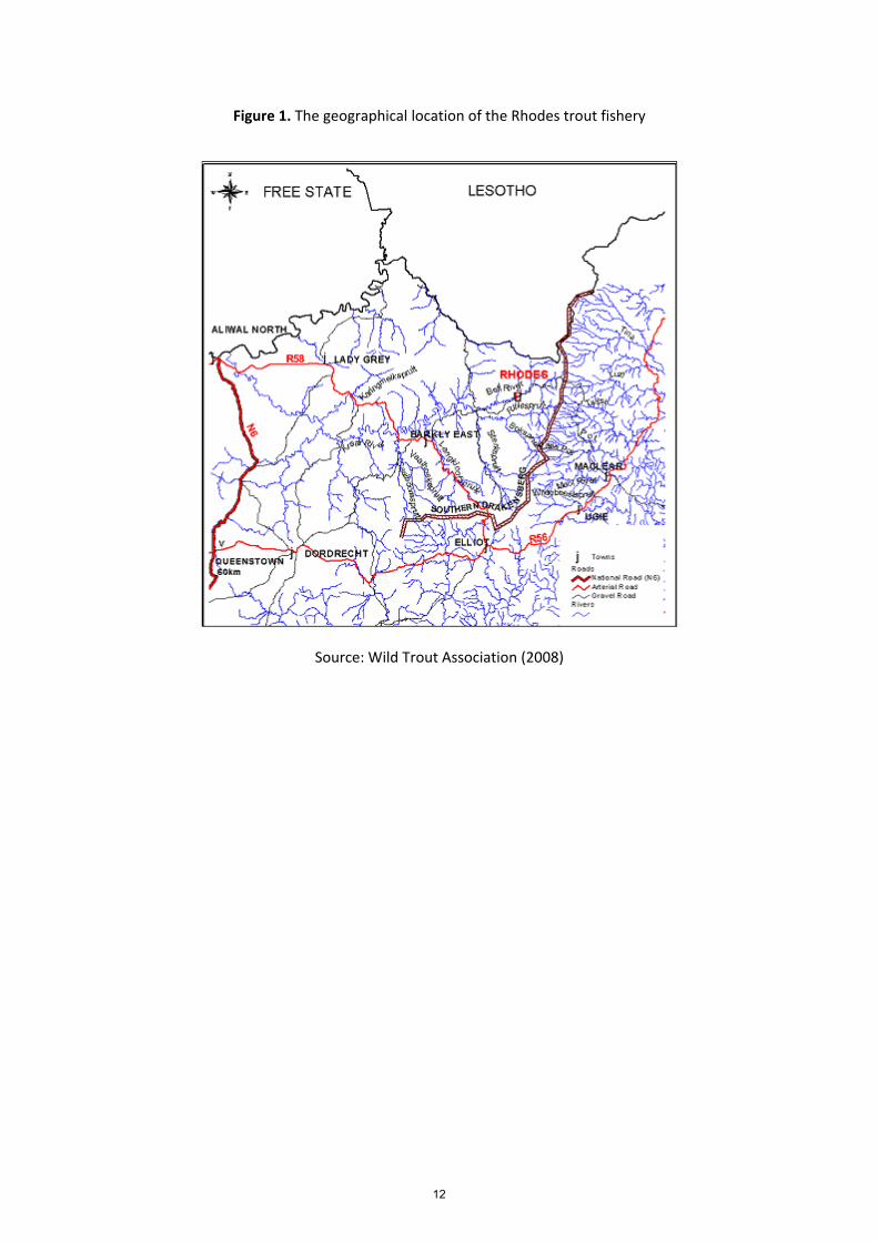
Figure 1. The geographical location of the Rhodes trout fishery 

 

Source: Wild Trout Association (2008) 

 

 

 

 

 

 

 

 

12

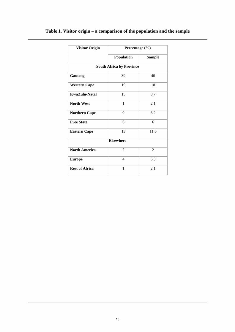
Table 1. Visitor origin – a comparison of the population and the sample

Visitor Origin Percentage (%)

Population Sample

South Africa by Province

Gauteng 39 40

Western Cape 19 18

KwaZulu-Natal 15 8.7

North West 1 2.1

Northern Cape 0 3.2

Free State 6 6

Eastern Cape 13 11.6

Elsewhere

North America 2 2

Europe 4 6.3

Rest of Africa 1 2.1

 

 

 

 

 

 

 

 

 

13

 

Table 2. Description of individual travel cost model variables 

 Variable name  Operational definition Expected 

sign 

Dependent variable 

Trips/annum  The number of trips per visitor per annum  

Independent variables 

Travel cost  Aggregate travel cost per visitor per visit (Rands) ‐ 

Travel time  Round trip travel time per visitor per visit (Hours) ‐ 

Gender  1= If gender is male

0=Otherwise 

+ 

Race  1=White 

0=Otherwise 

+ 

Catch  Aggregate number of fish caught in previous year + 

Age  Age of respondent (Years) + 

Income  Annual after‐tax income of respondent (Rands) + 

Substitute  Round trip travel time per visitor to favourite substitute site 

(Hours) 

+ 

 

14

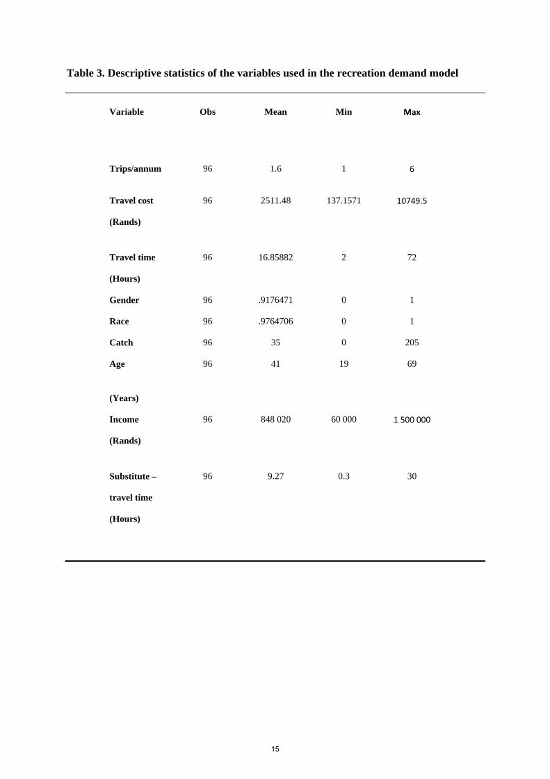
Table 3. Descriptive statistics of the variables used in the recreation demand model

Variable Obs Mean Min Max 

Trips/annum 96 1.6 1 6 

Travel cost

(Rands)

96 2511.48 137.1571 10749.5 

Travel time

(Hours)

96 16.85882 2 72

Gender 96 .9176471 0 1

Race 96 .9764706 0 1

Catch 96 35 0 205

Age

(Years)

96 41 19 69

Income

(Rands)

96 848 020 60 000 1 500 000 

Substitute –

travel time

(Hours)

96 9.27 0.3 30

 

 

 

 

 

15

 

Table 4. Recreational trout fishing demand model results 

Dependent

Variable

Poisson

Visits

∂Poisson

/∂X

ES Poisson

Visits - 1

∂ESPoisson

/∂X

NB

Visits

∂NB/∂X ZTNB

Visits

∂ZTNB/∂X

Travel cost -.0000717

(2.74)***

-.0005448 -.000085

(2.94)***

-.0005567 -.0000713

(1.83)*

-.000541 -.0000765

(1.83)*

-.0005689

Travel time -.0167321

(3.03)***

-.1270821 -.0190402

(3.19)***

-.1247006 -.0153518

(1.74)*

-.116727 -.0159899

(1.70)*

-.1189797

Gender .2481877

(1.63)

1.703771 .2859395

(1.74)*

1.667574 .1747044

(0.70)

1.236456 .1808346

(0.68)

1.249398

Race -.5248461

(2.39)**

-5.17779 -.5976927

(2.60)***

-5.282014 -.4420009

(1.06)

-4.18240 -.4591314

(1.04)

-4.289239

Catch .0024148

(6.07)***

.0183404 .0026394

(6.39)***

.0172862 .0023467

(2.54)***

.0178432 .0023841

(2.42)***

.0177398

Age .0005006

(0.13)

.0038023 .0005919

(0.15)

.0038763 .0014406

(0.23)

.0109532 .001682

(0.25)

.0125159

Income 6.59e-08

(0.75)

5.00e-07 7.43e-08

(0.79)

4.86e-07 1.50e-07

(0.93)

1.14e-06 1.66e-07

(0.97)

1.24e-06

Substitute .0088775

(2.99)***

.0674256 .0102117

(3.19)***

.0668799 .0084292

(1.73)*

.0640913 .0089061

(1.72)*

.0662699

Constant 2.463032

(8.42)***

2.383993

(7.67)***

2.354207

(4.42)***

2.339797

(4.15)***

Log-

L’hood

-281.8367 -291.2399 -241.3746 -239.75641

Pseudo R2 0.1153 0.1246 0.04 0.04

χ2 73.44*** 82.90*** 20.09*** 19.25***

AIC 581.6735 600.4798 502.7492 499.5128

BIC 603.6574 622.4637 527.1757 523.9393

Absolute value of z statistics in parentheses.

***, ** and * denote significance at 1%, 5%, and 10%, respectively.

16

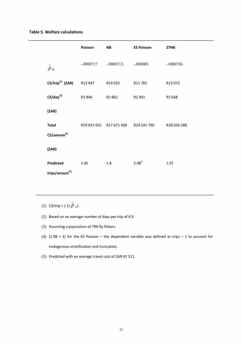
Table 5. Welfare calculations 

  Poisson  NB ES Poisson  ZTNB 

∧

β tc 

-.0000717 -.0000713

-.000085

-.0000765

CS/trip(1)  (ZAR) R13 947  R14 025 R11 765 R13 072 

CS/day(2) 

(ZAR) 

R2 846  R2 862 R2 401 R2 668 

Total 

CS/annum(3) 

(ZAR) 

R19 037 655 R17 671 500 R24 541 790 R18 026 288 

Predicted 

trips/annum(5) 

1.95  1.8 2.984 1.97 

 

(1) CS/trip = (‐1/ tc). ∧

β

(2) Based on an average number of days per trip of 4.9. 

(3) Assuming a population of 700 fly‐fishers. 

(4) (1.98 + 1)  for  the ES Poisson –  the dependent  variable was defined  as  trips – 1  to  account  for 

endogenous stratification and truncation. 

(5) Predicted with an average travel cost of ZAR R2 511.  

 

 

 

 

17