The Value of Earnings Comparability

Gus De Franco Rotman School of Management, University of Toronto

105 St. George Street Toronto, Canada, M5S 3E6

Phone: (416) 978-3101 Email: gus.defranco@rotman.utoronto.ca

S.P. Kothari

MIT Sloan School of Management 50 Memorial Drive E52-325 Cambridge, MA 02142-1347

Phone: (617) 253-0994 Email: kothari@mit.edu

Rodrigo S. Verdi

MIT Sloan School of Management 50 Memorial Drive E52-325 Cambridge, MA 02142-1347

Phone: (617) 253-2956 Email: rverdi@mit.edu

January 31, 2008

ABSTRACT

We develop a new metric of earnings comparability and study the capital market consequences of earnings comparability. The importance of comparability is expressed by regulators, teachers, practitioners, and researchers. The literature, however, lacks an empirical measure of financial statement comparability. More importantly, the “value” of comparability to users has not been established. We fill these gaps. We find that analyst following is increasing in earnings comparability, and that earnings comparability is positively associated with forecast accuracy and negatively related to bias in earnings forecasts. Our results suggest earnings comparability enhances a firm’s information environment.

______________________________ We appreciate the helpful comments of Rich Frankel, Wayne Guay, Jeffrey Ng, Ole-Kristian Hope, and workshop participants at MIT and University of Toronto, We thank I/B/E/S Inc. for the analyst data, available through the Institutional Brokers Estimate System. The data have been provided as part of their broad academic program to encourage earnings expectation research. We gratefully acknowledge the financial support of MIT and the Rotman School, University of Toronto. Part of the work on this article was completed while Gus De Franco was a Visiting Assistant Professor at the Sloan School of Management, MIT.

  1

The Value of Earnings Comparability

1. Introduction

Regulators, teachers, practitioners, and researchers all profess the importance of

“comparability.” According to the Securities and Exchange Commission (SEC) (2000), when

investors judge the merits of investments and comparability of investments, efficient allocation

of capital is facilitated and investor confidence nurtured. Financial statement analysis textbooks

almost invariably stress the need to compare calculated ratios to various benchmarks, including

ratios for the same firm in prior years, ratios for selected firms in the same industry, or ratios

based on industry averages.1 For instance, Stickney and Weil (2006) contend that, “Ratios, by

themselves out of context, provide little information.” In terms of research, there is also

considerable demand for control firms that “match” firms of interest. Despite the frequent use of

and the importance of comparability: 1) The literature lacks an empirical measure of financial

statement comparability; and, 2) The “value” of financial statement comparability to users is not

established in the literature.

We develop a measure of and study the capital market consequences of earnings

comparability. A key innovation is the development of an empirical, firm-specific, output-based,

quantitative measure of earnings comparability. We measure comparability based on financial

statement outputs. In particular, we restrict our comparability measure to (arguably) the primary

output of financial reporting: earnings. The measure is based on the strength of the historical

covariance between a firm’s earnings and the earnings of other firms in the same industry, as

evidenced by higher R2 values. While our primary focus is on creating a comparability measure

                                                            1 See, e.g., Libby, Libby and Short (2004), Stickney and Weil (2006), Stickney, Brown, and Wahlen (2007),

Revsine, Collins, and Johnson (2004), Wild, Subramanyam, and Halsey (2006), Penman (2006), White, Sondhi, and Fried (2002), and Palepu and Healy (2007).

  2

at the firm level, we also produce a measure of relative comparability at the “firm-pair” level, in

which a measure is calculated for all possible pairs of firms in the same industry.

Our measure is intended to capture comparability from the perspective of users, such as

investors or analysts, who need to evaluate historical firm performance, predict future firm

performance, or make other decisions using financial statement information. The measure

contrasts with qualitative, attribute-based definitions of comparability. For instance,

comparability can refer to comparable inputs such as similar business activities. Alternatively,

comparability could refer to a system which translates similar inputs to comparable outputs (e.g.,

accounting comparability). Thus, one caveat of our measure is that, although it is possible that

our output-based measure would be correlated with an input-based approach, it is not necessarily

so.

The study comprises two sets of empirical analyses. The first part describes our firm-

year measure of earnings comparability and provides descriptive properties of the measure.

Because it is new, we provide construct validity of our measure of earnings comparability. We

manually analyze the textual contents of a sub-sample of analysts’ reports. We find that the

likelihood of an analyst using another firm in the industry (say, firm j) as a benchmark when

analyzing a particular firm (say, firm i) is increasing in the relative comparability between the

two firms.

In the second part of the paper, we study the consequences of earnings comparability on

the firm’s information environment. Given a particular firm, we hypothesize that the availability

of information about similar firms (as captured by our earnings comparability measure) lowers

the cost of acquiring, and increases the overall quantity and quality of information available

about the firm. Our results are consistent with this idea. We find that firms with higher

  3

comparability are more likely to be followed by more analysts. In a more precise prediction, our

tests indicate that the likelihood of an analyst covering a particular firm (e.g., firm i) also

covering another firm in the same industry (e.g., firm j) is increasing in the relative comparability

between these two firms. These results suggest that the net benefits of higher earnings

comparability for analysts outweighs the potential diminished benefit of reduced investor

demand for a report on a firm that is highly comparable to another firm.

We also find that earnings comparability enables analysts to issue more accurate and less

biased earnings forecasts. Thus, earnings comparability helps analysts more accurately forecast

earnings and that the improvement comes, at least in part, through a reduction in forecast bias

(i.e., optimism). This result is consistent with more comparable firms providing a richer

information set. It is also consistent with acquiring information from sources other than

management, which reduces the reliance on managements’ private information, and hence

decreases the incentive for analysts to strategically add optimistic bias to forecasts. Last, we do

not find a significant relation between earnings comparability and forecast dispersion.

In some additional analysis, we construct a measure of stock return comparability that is

analogous to our earnings comparability measure. It is based on the covariance of historical

returns rather than earnings. We expect return comparability to better capture the economic

comparability across firms. Return and earnings comparability are positively correlated, which

provides additional validation and comfort that earnings comparability is in part explained by

economic comparability. We also replicate our information environment tests including both

earnings and return comparability in our regressions. Both the return and earnings comparability

relations are generally significant in the expected (and identical) directions. Hence, earnings

comparability is not subsumed by return comparability and must be capturing some differential

  4

effect. This result is consistent the existence of multiple dimensions of comparability, perhaps

an economic dimension that captures both long-term cash flow expectations and growth options

as well as a near-term, accounting-oriented dimension. It is also possible that both variables are

measuring a single underlying comparability construct with error.

Our study contributes to the literature in a number of ways. First, we develop a measure

of earnings comparability that likely captures user’s notions of comparability and the benefits of

comparability to them. We document tangible benefits for firms with higher comparability,

such as improved analyst coverage, and benefits for users of financial statements issued by more

comparable firms, such as improved forecasting. While comparability is generally and widely

accepted as a valuable trait, there is little evidence beyond this study proving this.

Second, our measure can be used to help evaluate whether a firm (or regulatory) action

that changes the economic transactions or the accounting of the transactions alters the

comparability, from a users point of view. For example, according to the International

Accounting Standards Committee Foundation (IASCF), the primary objective of the

International Financial Reporting Standards (IFRS) is to develop a single set of “global

accounting standards that require high quality, transparent and comparable information in

financial statements and other financial reporting” (IASCF 2005). Our measure could be used to

assess whether IFRS achieves the intended consequence of enhanced financial statement

comparability (see e.g., Beuselinck, Joos, and Van der Meulen, 2007). More broadly, our

measure can be used to assess the changes in earnings comparability as a result of changes in

accounting earnings measurement rules or reporting standards, accounting choice differences, or

of adjustments.

Third, researchers might use our measure of earnings comparability to help design more

  5

powerful tests. For instance, prior research highlights the importance of properly controlling for

certain firm characteristics when testing hypotheses related to firm performance and earnings

management (Barber and Lyon, 1996, 1997; Kothari, Leone, and Wasley, 2004). Our measure

of earnings comparability could be used in this context to help identify a set of ‘comparable’

firms.

Last, our measure could assist practitioners, such as analyst and boards, in objectively

choosing their choice of comparable firms. Currently, choosing comparables is often considered

an “art form” (see Bhojraj and Lee, 2002) and the inherent discretion in this choice can lead to

strategic behavior. For example, Lewellen, Park, and Ro (1996) show that firms’ choices of

industry and peer-company benchmarks are self serving. Thus, our measure could be used

internally by firms or externally by investors to assess or validate this choice.

The paper proceeds as follows. Section 2 defines our earnings comparability measure

and provides construct validity tests of the measure. Section 3 outlines our predictions that

earnings comparability improves a firm’s information environment. Section 4 presents the

results of our tests. Section 5 provides some additional analysis that incorporates the return

comparability measure. The last section concludes.

2. A measure of earnings comparability

In this section, we first describe the demand for comparable information and then explain

how we compute our measure of earnings comparability. In addition, since our measure of

earnings comparability is novel, we provide descriptive information on the measure’s properties

to ascertain the measure’s construct validity.

  6

2.1. Demand for comparable information

Comparability is widely accepted as a desirable attribute. From a regulatory perspective,

in addition to the views of the SEC, the usefulness of comparable financial statements is

underscored in the Financial Accounting Standards Board (FASB) accounting concepts

statement. Specifically, the FASB (1980, p. 40) states that “investing and lending decisions

essentially involve evaluations of alternative opportunities, and they cannot be made rationally if

comparative information is not available” (Our emphasis). Comparability is also one of three

qualitative characteristics of accounting information included in the accounting conceptual

framework (along with relevance and reliability). Further, according to the FASB (1980, p. 40),

“The difficulty in making financial comparisons among enterprises because of the different

accounting methods has been accepted for many years as the principal reason for the

development of accounting standards.” Here, the FASB argues that users’ demand for

comparable information drives accounting regulation.

In terms of teaching and practice, there is significant demand for benchmarks to evaluate,

predict, or justify a number or ratio. Penman (2006) states: “To make judgments about a firm’s

performance the analyst needs benchmarks. Benchmarks are established by reference to other

firms (usually in the same industry) or to the same firm’s past history.” Koller et al. (2005)

contend that a carefully designed price multiples analysis can provide valuable insights about the

company and its competitors, and recommend that analysts choose firms with similar prospects.

In addition, the actual use of price multiples in valuation by sell-side analysts is ubiquitous

(Bhojraj and Lee, 2002; Asquith et al., 2005). This drives demand for comparable firms that

help analysts to evaluate and predict future price multiples. Last, firms must report to regulators

  7

a comparison of their stock performance with a set of comparable firms or an index as

benchmarks for compensation purposes (see, e.g., Lewellen, Park, and Ro, 1996).

In terms of research, there is demand to control for firms’ underlying economics. This is

often done by including industry fixed effects, so that the analysis focuses on within-industry

variation or by using a matched-pair design. These control firms are often chosen such that

industry, size, book-market ratios, and the previous year’s financial performance are similar to

the treatment firm (see, e.g., Barber and Lyon 1996, 1997; Kothari, Leone and Wasley, 2005).

There could also be demand in terms of contracting research. For example, Albuquerque (2006)

finds that improvements in determining who peer firms are improves the ability to identify

relative performance evaluation.

2.2. Measuring earnings comparability

The term comparability in accounting textbooks, in regulatory pronouncements, and in

academic research is defined broadly and imprecisely. For instance, comparability could refer to

comparable inputs such as similar accounting methods, business activities, or industry

membership. As an example, Bradshaw and Miller (2007) study whether firms that intent to

harmonize their accounting with US GAAP change to US GAAP accounting methods. DeFond

and Hung (2003) argue that accounting choice heterogeneity (e.g., differences in inventory

methods such as LIFO versus FIFO) increases the difficulty in comparing earnings across firms.

Alternatively, comparability might be defined as a function of outputs such as similar earnings

and financial ratios. We adopt the perspective of a user of financial statements, such as an

investor or analyst, and focus on financial statement outputs. In particular, we develop our

measure of comparability using one primary output of financial reporting, namely, earnings. Our

  8

user perspective is important and consistent with the benefits we analyze (discussed below),

which are from the perspective of users (in particular, financial analysts).

We begin by proposing a measure of comparability that is intuitively consistent with the

definition of comparability implicit in accounting standards and the professional literature on

financial statement analysis. As mentioned above, we teach and emphasize in any lesson on

financial statement analysis that it is difficult to draw meaningful inferences about a financial

measure unless there is a “comparable” benchmark. FASB (1980, p. 40) echoes this point.

Implicit is the idea that better benchmarks produce better inferences (e.g., better evaluation of

firm performance, better prediction of next year’s price-multiple, etc.). We expect that similar

firms will provide better benchmarks for each other. Hence the quality of information is higher.

As an additional consideration, the expectation of information transfer among similar firms is

also much higher. Thus the cost of acquiring information is lower.

To identify similar firms, we calculate the historical covariance of quarterly earnings

between all possible pairs of firms in the same industry. We sort firms based on the ability of

other firms’ earnings to predict the respective firm’s earnings. Ceteris paribus, firms with higher

comparability are firms in which earnings covary more with the earnings of other firms in the

industry, as evidenced by higher R2 values. If firms are similar, they are more likely to

experience similar economic shocks. For instance, a change in input prices or shifts in consumer

demand for firms with similar business models should translate into similar changes in economic

profitability. These firms are also likely to account for economic transactions in a similar way.

In contrast, if business models are different, or firms are sensitive to different types of shocks, or

the accounting is different, then we would not expect to see earnings covary over time.

More specifically, earnings comparability is defined as follows. We first estimate:

  9

Earningsijt = Ф0ij + Ф1ij Earningsjt + εijt. (1)

We measure Earnings as the ratio of quarterly net income before extraordinary items (data8) to

the average total assets (data44), taken from the Compustat Quarterly file. To determine the

most comparable firm j for each firm i, we estimate Equation (1) for each firm i – firm j pair, (i ≠

j), j = 1 to J firms in the same 2-digit SIC industry with available data. We require 16 quarters of

data available for each firm i – firm j combination and we estimate Equation (1) at the end of

December for each year. We also restrict the sample to firms whose fiscal year ends in March,

June, September, or December. This ensures that i and j firms’ earnings are measured at the end

of the same fiscal quarter. In order to avoid the influence of outliers, we remove observations in

which Earnings for firm i is more than three standard deviations from the mean value of the 16

Earnings observations for firm i used to estimate Equation (1).

After estimating the R2 for regression model (1) for each firm i – firm j combination, we

rank all J values of R2s for each firm i from the highest to lowest R2. The most comparable firm

is the one that produces the highest R2. Comp4 is the average R2 for the four firms with the

highest R2. CompInd is the average R2 for all firms in the industry.2 These are the two

comparability measures we use in our tests. The idea is that firms with high Comp4 and

CompInd are firms for which earnings variation is better explained by variation in the earnings of

other firms in the same industry.

Before proceeding further, we discuss measures used in other studies that are indirectly

related to ours. First, existing measures of comparability in the literature are based mainly on

similarities in cross-sectional levels of contemporaneous measures (e.g., return on equity, firm

                                                            2 Admittedly, the choice of how many firms should be included in the set of comparable firms is ad hoc. In

untabulated analyses, we use the R2 from the single most comparable firm as well as the average R2 from the top ten firms. The results for the single most comparable firm seem to be slightly weaker, while the results for the top ten firms are similar to using the top-four firms.

  10

size, price multiples) at a point in time. Joos and Lang (1994) study the comparability of

accounting data in a European setting. They expect that improved accounting comparability

between countries will result in smaller differences between accounting measures of profitability

(i.e., ROE), between valuation multiples of accounting data (i.e., Earnings/Price; Book

value/Market value of equity), and between the degree of association between accounting and

stock data (i.e., value relevance). Land and Lang (2002) also focus on comparing valuation

multiples across countries. These measures are typically estimated in aggregate at the country

level. Another set of literature attempts, for each treatment firm, to find the closest matching

firm. This is often done by restricting the set of matched firms along certain dimensions, such as

similar industry, size quintiles, etc. and perhaps minimizing the distance along a particular

dimension such as return on equity (see, e.g., Barber and Lyon 1996, 1997; Kothari, Leone and

Wasley, 2005). Our measure is more dynamic, capturing similarities in co-variation over time,

and is firm-specific.3

Second, our measure of earnings comparability is related to the previously-established

time-series concept of earnings “predictability” in which earnings are regressed on previous-

period earnings (e.g., Lipe 1990). We estimate firms’ predictability from the following time-

series model (this measure is used below in our tests):

Earningsit = Ф0i + Ф1i Earningsit-4 + εit. (2)

The model is estimated for each firm i over a rolling 16-quarter window.4 Predictability is

defined as the R2 from Equation (2). This is a firm-specific measure of predictability.

                                                            3 Interesting exceptions are studies that examine the returns to pairs trading, such as Papadakis and Wysocki

(2007). They identify pairs of similar firms using the average difference in daily “normalized” price over a 12-month period. In effect, their measure captures a blend of similar levels and similar covariation over time.

4 We focus on quarterly predictability, which aligns with our earnings comparability measure derived from quarterly earnings. Much of the prior research focuses on annual predictability, typically estimated per firm over a rolling 10-year window using annual earnings (Lipe 1990; Francis, LaFond, Olsson, and Schipper, 2004).

  11

Predictability, all else equal, is desirable since one important task investors perform is

forecasting future earnings for the purpose of valuing their securities. In essence, our earnings

comparability measure is a cross-sectional version of predictability. While earnings predictability

or persistence measures have been around in the literature for quite some time (see, e.g., Lipe

1990, and Francis, LaFond, Olsson, and Schipper, 2004), their use in developing a comparability

measure in this study is unique.

Third, Piotroski and Roulstone (2004), and Chan and Hameed (2006), among others,

study stock price synchronicity, which is based on the R2 from a regression of firm’s stock

returns on market and industry stock returns. They are inherently interested in the type of

information (firm, industry, or market) impounded in stock prices. We highlight that our

measure is based solely on accounting data, and is hence not sensitive to flows of non-accounting

information, to investor’s interpretation, or to assumptions about market efficiency. Our

measure could also be applied to private firms.

Fourth, an older literature studies the accounting beta, which captures the relation

between earnings at the firm level and earnings at the industry or market level. Brown and Ball

(1967) show that firm earnings can be explained in part by the earnings of other firms in the

same industry and the earnings of all firms in the market. This research focuses on documenting

that the market beta (from a capital asset pricing model) is positively related to the accounting

beta (see, e.g., Beaver, Kettler, and Scholes 1970; Beaver and Manegold 1975; Gonedes 1973,

1975).

2.3. Sample and descriptive statistics

To estimate earnings comparability, we obtain quarterly accounting data from Compustat

starting in 1991. As discussed above, we require 16 quarters of net income before extraordinary

  12

items data for a given firm i (in addition to 16 quarters for firm j). We exclude holding firms. In

some cases, Compustat contains financial statements for both the parent and the subsidiary

company, and we want to avoid matching such two firms. We exclude ADRs and limited

partnerships because our focus is on corporations domiciled in the United States.5 We also

exclude firms that have names highly similar to each other using an algorithm that matches five-

or-more-letter words in the firm names, but avoids matching on generic words such as “hotels”,

“foods”, “semiconductor”, etc. Finally, we restrict the sample to industries with at least 20 firms

per year based on the SIC two-digit classification. These restrictions result in a sample of 42,336

firm years (about 3,500 firms per year) with available data to estimate earnings comparability

during 1994 to 2005. In addition, in our later analysis we restrict the sample to firms followed

by analysts. We use data from IBES for all our analyst measures. This restriction reduces the

sample to 20,508 firm-year observations with the comparability score and analyst coverage. We

term the former the unrestricted sample and the latter the analyst-restricted sample. The analyst-

restricted sample is biased towards larger and more-frequently-trading firms.

Table 1 presents descriptive statistics for our measure of earnings comparability. Panel A

presents the number of observations and the means for Comp4 and CompInd by year for the

unrestricted and analyst-restricted samples. The mean value for Comp4 ranges from 50.3% to

54.5% for the unrestricted sample. For the average firm in our sample, the four firms in the same

industry with the highest earnings correlation explain about half the variability of the sample

firm’s earnings. Likewise, the CompInd mean, i.e., the average R2 for Equation (1) for all firms

in the industry is about 11-12%. The results are similar for the analyst-restricted sample except

that the comparability scores are slightly higher.

                                                            5 Specifically if the word Holding, Group, ADR, or LP (and associated variations of these words) appear in the

firm name on Compustat, the firm is excluded.

  13

[Table 1]

Panel B presents descriptive statistics for the unrestricted sample. We note that Comp4

and CompInd present considerable cross-sectional variation. For instance, the 10th percentile and

the 90th percentile for Comp4 equal 32.5% and 73.6%, respectively. In addition, for comparison,

Panel B also presents descriptive statistics for Predictability, which is defined as the R2 of a

regression of earnings on prior-year earnings as described in Equation (2). In this case, the mean

predictability score is 15.9% which means that for the average firm in the sample, prior earnings

explain about 16% of the variability in one-year ahead earnings. Finally, Panel C presents

Pearson correlations among the three variables. As expected, the two comparability measures

are highly correlated (correlation coefficient of 0.71). In addition, comparability is also

positively correlated with firm predictability.

2.4. Validating our earnings comparability measure

In this section, we describe a test aimed at providing construct validity of our earnings

comparability measure. An assumption implicit in this test is that, for any given firm, investors

and analysts know the identity of comparable firms (if any). Investors and analysts have access

to a broad information set about each firm, which goes beyond the historical financial statements,

and includes firms’ business models, competitive positioning, markets, products, etc. While the

actions and analyses of investors might be largely private, analysts’ output (e.g., earnings

forecasts) and analyses (e.g., their reports) are observable. Hence, our tests focus on analysts.

We provide a testable prediction to establish our measure’s construct validity. This

prediction relates to the important assumption underlying our measure, namely, that the ranking

of R2s from pairwise firm i - firm j regressions in fact identifies a set of comparable firms for

firm i. We predict that if an analyst issues a report about firm i, then we expect her to more

  14

likely use firms that are “comparable” to firm i in her reports. The typical analyst report context

is that the analyst desires to evaluate the current, or justify her predicted, firm valuation multiple,

(e.g., Price/Earnings ratio), using a relative analysis of similar firms’ valuation multiples as

benchmarks. Evidence from a test of this prediction suggests our assumption is valid.

The comparable firms that an analyst uses in her analysis are not available in a machine-

readable form in existing databases. We hand collect a sample of analyst reports from Investext

and manually extract this information from the reports. The cost of hand collecting this

information limits the size of this sample. Reports are chosen as follows. We randomly select

350 firms (i.e., firm i’s) in our sample with available data for the year 2005. For these firms, we

search Investext to find up to three reports per firm i, each report written by a different analyst,

that refer to “comparable” or “peer” firms (i.e., potential firm j’s) in the report. We then record

the name and ticker of all firms used by the analyst as a peer or comparable firm for firm i. We

match these peer firms with Compustat using the firm name and ticker. In total, we obtain 150

reports written by 126 unique analysts for 98 unique firms. Each report mentions one or more

firms as comparable to the firm for which the analyst has issued the report.6

For our tests, we estimate the following logistic regression:

UseAsCompikj = α + β1 ijRSQij + γ Controlsj + εikj. (3)

UseAsComp is an indicator variable that equals one if analyst k who writes a report about firm i

refers to firm j as a comparable firm in her report, and equals zero otherwise. ijRSQ is the R2

from the estimation of Equation (1) for each firm i – firm j pair in our sample. We predict that

the probability of an analyst using firm j in her report is increasing in ijRSQ. We use Size,

                                                            6 Part of the reason this process is labor intensive is because we do not know ex ante whether Investext covers

firm i, and because not all analysts discuss comparable firms in their analysis. For example, many reports represent simple updates with no discussion of valuation methods. In other cases, analysts rely more heavily on a discounted flow analysis or use historical valuation multiples to predict future multiples. We exclude reports on Investext that are computer generated or not written by sell-side analysts.

  15

Volume, Book-Market, ROA, and industry fixed effects as control variables. Our choice of these

controls follows their common use by other researchers who match control firms with treatment

firms along these three dimensions (see, e.g., Barber and Lyon, 1996, 1997; Kothari, Leone, and

Wasley, 2005). In addition to the levels of these variables, we control for the differences in

characteristics between firm i and firm j. The intuition for using both levels and differences is as

follows: An analyst who reports on firm i is more likely to use a firm as a peer if the firm has

similar (comparable) characteristics (e.g., similar size, growth potential and profitability) to firm

i. This implies the larger the difference between firm i and firm j, the less likely it is to be

covered by the analyst. However, large, high-growth, and highly-profitable firms are more likely

to be covered by an analyst and recognized by investors, which motivates us to also include the

levels of these firm characteristics in the regression.

Table 2 presents the logistic regressions for model (3). The coefficient on ijRSQ is

positive and statistically significant in both columns as predicted. This suggests that as the ijRSQ

increases, it increases the odds of an analyst using firm j as a peer firm in a report about firm i.

While the coefficients on Book-Market and ROA are not significant, the coefficients on Size and

Volume are positive and statistically significant. In addition, the estimated coefficients of the

differences in the control variables between firm i and firm j are all negative and significant

suggesting that analysts tend to more likely use firms as peers if they are similar along these

dimensions.

[Table 2]

Overall, the results in Table 2 support the notion that an analyst who writes a report about

a firm will more likely choose benchmark firms that have higher values of our earnings

  16

comparability measure. This bolsters the construct validity of our earnings comparability

measure.

3. Hypotheses: Capital market consequences of earnings comparability

In this section, we develop hypotheses about the capital market consequences of earnings

comparability. As mentioned above, while we are interested in both investors and analysts,

given the rich publicly-available information on analysts, we focus on their outputs (i.e., earnings

forecasts). We predict that higher earnings comparability lowers analysts’ cost of understanding

the firm and evaluating its performance. In addition, we expect the net information set for

comparable firms to be of higher quantity and quality. This richer information set facilitates

analysts’ ability to forecast firm i’s earnings when these other firms are comparable. Hence, we

expect that in the cross-section, higher comparability will be associated with better information

environments. We investigate two dimensions of analysts’ behavior – the number of analysts

following a firm and the properties of analyst forecasts.

Our first hypothesis examines whether comparability affects analyst coverage. As

discussed in Bhushan (1989) and in Lang and Lundholm (1996), the number of analysts

following a firm is a function of the analysts’ costs and benefits. We argue that, ceteris paribus,

because firms with higher comparability have richer information sets, it is easier to analyze these

firms, and so more analysts should cover these firms. Our first hypothesis (in alternate form) is:

H1: Ceteris paribus, earnings comparability is positively associated with analyst coverage.

An argument consistent with the null hypothesis is that the better information

environment associated with higher-comparability firms will decrease the investor demand for

analyst coverage. That is, the benefits to analysts will decrease as well. However, the literature

  17

on analysts suggests that analysts primarily interpret information as opposed to convey new

information to the capital markets (Lang and Lundholm 1996; Francis, Schipper, and Vincent

2002; Frankel, Kothari, and Weber, 2006; De Franco, 2007). As a specific example, Lang and

Lundholm (1996) find that analyst coverage is increasing in firm disclosure quality. These

empirical findings suggest that an increase in the supply of information results in higher analyst

coverage, consistent with the lower costs of more information outweighing the potentially lower

benefit of decreased demand. These findings in the literature support our signed prediction.

Our second set of hypotheses examines the association between earnings comparability

and the properties of analyst earnings forecasts. The first property we examine is forecast

accuracy. To the extent that comparability facilitates investors’ ability to forecast firm i's

earnings the accuracy of earnings forecasts should, ceteris paribus, increase with earnings

comparability. For example, the existence of comparable firms could allow analysts to better

explain firms’ historical performance or to use information from comparable firms as an

additional input in their earnings forecasts. Our hypothesis 2a (in alternative form) is:

H2a: Ceteris paribus, earnings comparability is positively associated with analyst forecast accuracy.

Second, prior research finds analysts’ long-horizon forecasts are optimistic on average

(e.g., O’Brien, 1988, and Richardson et al., 2004).7 Francis and Philbrick (1993), Das et al.

(1998), and Lim (2001) show that part of the bias in analyst forecasts is explained by analysts

adding optimism to their forecasts to gain access to management’s private information, which

helps improve forecast accuracy.8 If information from comparable firms serves as a substitute

for managements’ private information, then the incentive to strategically add optimistic bias to

                                                            7 Analyst optimism has decreased over time and is more-pronounced for longer-horizon forecasts and it seems

to be driven by relatively few observations (Brown 2001; Lim 2001; Gu and Wu 2003; Richardson et al. 2004). 8 Recent research by Eames et al. (2002) and Eames and Glover (2003) question these results.

  18

gain access to management is reduced. Further, if more objective information from comparable

firms is available, it is easier to identify when (i.e., catch) analysts act strategically, which hence

increases the cost to the analyst of this behavior. Therefore analysts’ forecasts of higher-

comparability firms should be less optimistic. We state this prediction as hypothesis 2b (in

alternate form):

H2b: Ceteris paribus, earnings comparability is negatively related to analyst forecast optimism.

Third, we investigate the relation between earnings comparability and analyst forecast

dispersion. If analysts have the same forecasting model, and if higher comparability implies the

availability of superior public information, then an analyst’s optimal forecast will place more

weight on public information and less on her private information. This implies comparability

will reduce forecast dispersion. Our hypothesis 2c (in alternative form) is:

H2c: Ceteris paribus, earnings comparability is negatively associated with forecast dispersion.

We acknowledge that superior public information via higher comparability could

generate more dispersed forecasts, which would support the null of hypothesis 2c. The intuition

here is that if analysts process a given piece of information differently from other analysts, then

the availability of greater amounts of public information for comparable firms will generate more

highly-dispersed forecasts. At least two theoretical studies predict such a phenomenon. Harris

and Raviv (1993) and Kandel and Pearson (1995) develop models in which disclosure promotes

divergence in beliefs. Kim and Verrecchia (1994) allow investors to interpret firm disclosures

differently, whereby better disclosure is associated with more private information production.

  19

4. Empirical Tests

4.1. Analyst coverage tests

To test whether analyst coverage and comparability are positively related, our first

hypothesis, we estimate the following regression:

Coverageit+1 = α + β1 Comparabilityit + β2 Predictabilityit + γ Controlsit + εit+1. (4)

Coverage is the logarithm of the number of analysts issuing an annual forecast for firm i in year

t. Comparability is either Comp4 or CompInd. We include Predictability in our specification

because it represents a natural benchmark to assess the economic significance of our

comparability measure. Predictability is based on a statistical model, like comparability. More

importantly, predictability is accepted in the literature as a desirable earnings attribute (Schipper

and Vincent, 2003; Francis et al., 2004).

In estimating model (4), we control for other factors motivating an analyst to cover firm j

by including the determinants of analyst coverage previously documented in the literature (e.g.,

Bhushan, 1989, O’Brien and Bhushan, 1990, Brennan and Hughes, 1991, Lang and Lundholm,

1996, and Barth, Kasznik, and McNichols, 2001). Size is the logarithm of the market value of

equity measured at the end of the year. Volume is the logarithm of trading volume in millions of

shares during the year. Issue is an indicator variable that equals one if the firm issues debt or

equity securities during the years t-1, t, or t+1, and zero otherwise. Book-Market is the ratio of

the book value to the market value of equity. R&D is research and development expense scaled

by total sales. Depreciation is depreciation expense scaled by total sales. Throughout the

remaining analysis, for continuous variables that we do not take the logarithm of, we delete

observations if these variable values fall in the lowest or highest percentile of their respective

distributions, calculated annually (i.e., we trim the data annually at the 1% and 99% percentile).

  20

We also include industry and year fixed effects. Because the estimation of Equation (4) is likely

to suffer from time-series dependence, we estimate the model as a panel and cluster the standard

errors at the firm level (in addition to the year fixed-effects).

As seen in Table 1, we have 20,508 firm years with comparability scores in the analyst-

restricted sample. In order to test hypothesis 1, we further restrict the sample to firms with

available data to compute the control variables. This reduces the sample to 18,735 firm-year

observations from 1994 to 2005.

Table 3, Panel A presents descriptive statistics for the variables included in this analysis.

An average (median) firm in our sample is covered by 7 (4) analysts (see the variable Coverage-

N, which is the number of analysts issuing a forecast for the firm). The mean value for Comp4

(CompInd) is 0.55 (0.12), which is similar to the means of these variables presented in Table 1.

Turning to the control variables, the average firm in the sample has a market value of $2.7 billion

(see the variable Size-$M, which is the firm’s market value of equity measured in $millions) and

a Book-Market of 0.54. Panel B presents the correlation matrix. Consistent with prior research

we find that Coverage is positively correlated with firm size and trading volume, and is

negatively correlated with the book-market ratio. More importantly, Coverage is positively

correlated with both measures of earnings comparability.

[Table 3]

Table 4 presents the regression results. Both of the earnings comparability measures are

positively associated with analyst coverage and the results are robust to the inclusion of earnings

predictability in the model. In terms of economic significance, an increase from the 10th to the

90th percentile in Comp4 (CompInd) is associated with an increase of 0.40 (0.35) analysts. Given

that the median coverage in our sample is four analysts this represents an increase of almost

  21

10%, suggesting that the effect is also economically significant. Consistent with prior research,

we find that analyst following is increasing in firm size and trading volume. However, we find

an inconsistent coefficient for Book-Market. Overall, the regression results in Table 4 confirm

the univariate findings in Panel B of Table 3, and are consistent with hypothesis 1 that predicts a

positive association between analyst coverage and earnings comparability. It suggests the net

benefits of covering firms with high comparability (due to the richer information environment)

outweigh the potential decreased benefit from investors’ reduced demand for information about

highly-comparable firms.

[Table 4]

4.2. Analyst coverage of other firms conditional on covering a particular firm

We now provide additional evidence of higher analyst coverage, our first hypothesis, in

the form of a more precise prediction about which firms an analyst will cover. We expect that the

likelihood of an analyst covering a particular firm (e.g., firm i) also covering another firm in the

same industry (e.g., firm j) is increasing in the relative comparability between these two firms.

Hence, we not only predict that higher earnings comparability leads to more analysts covering

the firm, but also specifically predict which other firms the analyst will follow.

We estimate the following logistic regression for each year of our sample:

CondCoverageikj = α + β1 ijRSQij + γ Controlsj + εikj. (5)

CondCoverage is an indicator variable that equals one if analyst k who covers firm i also covers

firm j, and equals zero otherwise. An analyst “covers” a firm if she issues at least one annual

forecast about the firm. We predict that the probability of covering firm j is increasing in ijRSQ.

We use the same variables as in Equation (4) to control for other factors that could explain

analyst coverage (but measured for firm j).

  22

The annual sample for this test is quite large. For firm i, there are K analysts who cover

the firm. For each firm i – analyst k pair there are J firms in the same industry as firm i. Hence,

our sample consists of I firms × K analysts × J firms. In addition to requiring valid data for all

our measures, we require each analyst k to cover at least five firms. In estimating the model, we

rely on the coverage choice of an analyst within an industry, and therefore require the availability

of at least a few observations per analyst per industry for which CondCoverage equals one. This

restriction should exclude junior analysts, analysts in transition, and data-coding errors. We

exclude analysts who cover more than 40 firms. Covering greater than 40 firms is rare (less than

one percent of analysts) and could be a data-coding error in that the observations could refer to

the firm employing the analyst rather than an individual analyst at the firm.

In Table 5, we provide the mean, maximum, and minimum coefficient from the 12 annual

logistic regressions. The large sample size (average annual sample used in our tests consists of

2,904,641 firm i – analyst k – firm j observations) prohibits us from estimating a panel

regression. The mean coefficient t-statistic is based on the distribution of the 12 annual

coefficients using the Fama and MacBeth (1973) procedure. Further, we adjust for potential

time-series dependence in the estimates using the Newey-West (1987) correction with one lag

(In untabulated tests we find that higher lags lead to higher t-stats. Thus we present the

conservative estimate.). The mean coefficient on ijRSQ is positive and statistically significant as

predicted. In addition, the coefficient is positive in all 12 years. The result suggests that the firm

j’s we identify as “comparable” to firm i are more likely to be followed by the analysts who also

cover firm i. The coefficients on the control variables generally correspond with the direction

documented in the literature. For example, analyst coverage is increasing in firm size, trading

volume, research and development, and depreciation.

  23

[Table 5]

Overall, the results in Table 5 present evidence that the likelihood of an analyst covering firm

j, conditional on the analyst covering firm i, is increasing in the extent of the comovement of the

earnings of firms i and j, i.e., the pair-wise earnings R2. This provides additional evidence

consistent with higher comparability of earnings reducing the cost of covering the firm.9

4.3. Forecast accuracy, optimism, and dispersion tests

To test our hypotheses about whether comparability affects forecast accuracy, optimistic

bias, and dispersion, we estimate the following specification:

Forecast Metricit+1 = α + β1 Comparabilityit + β2 Predictabilityit + γ Controlsit + εit+1. (6)

Forecast Metric is Accuracy, Optimism, or Dispersion. Analyst forecast accuracy is the absolute

value of the forecast error multiplied by -1:

Accuracyit = |Fcst EPSit – Actual EPSit|/Priceit-1 × -1. (7)

Fcst EPSit is analysts’ mean I/B/E/S forecast of firm-i’s annual earnings for year t. For a given

fiscal year (e.g., December of year t+1) we collect the earliest forecast available during the year

(i.e., we use the earliest forecast from January to December of year t+1 for a December fiscal

year-end firm). Actual EPSit is the actual amount announced by firm i for fiscal period t+1 as

reported by I/B/E/S. Price is the stock price at the end of the prior fiscal year. Because the

absolute forecast error is multiplied by -1, higher values of Accuracy imply more accurate

forecasts.

We measure optimism in analysts’ forecasts using the signed forecast error:

Optimismit = (Fcst EPSit – Actual EPSit)/Priceit-1. (8)

                                                            9 This result is related to a study by Ramnath (2002) who shows that there is information transfer between firms

covered by the same analyst. He shows that among these firms, the earnings announcement surprises of firms that announce first are systematically related to forecast revisions for the other firms that the analysts cover.

  24

Dispersion is the cross-sectional standard deviation of individual analysts’ annual forecasts for a

given firm, scaled by price. Hypothesis 2 predicts that accuracy is increasing in earnings

comparability, and that optimism and dispersion are decreasing in earnings comparability.

We control for other determinants of these forecast metrics as previously documented in

the literature. SUE is the absolute value of firm i’s unexpected earnings in year t scaled by the

stock price at the end of the prior year. Unexpected earnings are actual earnings minus the

earnings from prior year. Firms with greater variability are more difficult to forecast, so forecast

errors should be greater (e.g., Kross, Ro and Schroeder, 1990, and Lang and Lundholm, 1996).

Consistent with Heflin, Subramanyam and Zhang (2003), earnings with more transitory

components should also be more difficult to forecast. We include the following three variables

to proxy for the difficulty in forecasting earnings. Neg UE equals one if firm i’s earnings are

below the reported earnings a year ago, zero otherwise. Loss equals one if the current earnings is

less than zero, zero otherwise. Neg SI equals the absolute value of the special item deflated by

total assets if negative, zero otherwise. We expect these three variables to be positively related

to optimism given that optimism is greater when realized earnings are more negative.

Daysit is a measure of the forecast horizon, calculated as the logarithm of the number of

days from the forecast date to firm-i’s earnings announcement date. The literature shows that

forecast horizon strongly affects accuracy and optimism (Sinha et al., 1997, Clement, 1999, and

Brown and Mohd, 2003). Last, we include industry and year fixed effects. Similar to the

estimation of Equation (4), we estimate the model as a panel and cluster the standard errors at the

firm level.

After computing forecast accuracy and the control variables for these tests, the final

sample is reduced to 17,178 firm-year observations. The final sample is smaller still for the tests

  25

of dispersion because the standard deviation requires at least 3 analysts for a given firm. Table 6

presents descriptive statistics (Panel A) and the correlation matrix (Panel B) for the variables

included in the analysis. Mean accuracy is 4.2% of share price. Mean optimism is 2.5% of share

price, which is consistent with prior research that analysts tend to be optimistic on average.

However, the median is only 0.2%, also consistent with previous research. The mean forecast

dispersion is 0.7% of share price. In terms of correlations, we find that the earnings

comparability measures are positively correlated with forecast accuracy, and negatively

correlated with forecast bias.

[Table 6]

Table 7 presents the regression results for all three forecast metrics. The first two

columns present results for forecast accuracy. With respect to the earnings comparability

measures, our primary variables of interest, we find that comparability is positively associated

with accuracy. In terms of economic significance, an increase from the 10th to the 90th percentile

in Comp4 (CompInd) is associated with an increase in accuracy of about 0.67% (0.45%). This

represents an improvement in accuracy of about 10-15% for the average firm in the sample. This

result supports hypothesis 2a that higher earnings comparability increases the accuracy of

analysts’ forecasts. With respect to the control variables, we find that forecast accuracy is

positively associated with earnings predictability. Further, accuracy is decreasing in the

incidence of losses and in the variability of earnings. In addition, forecast accuracy is also

decreasing in the forecast horizon (i.e., the time between forecast and announcement date).

[Table 7]

The next two columns in Table 7 present the results for forecast optimism. In this case,

we find that analyst optimism is greater for firms reporting losses or firms reporting a decrease in

  26

earnings, consistent with our predictions. As with forecast accuracy, the result is also

economically significant suggesting a reduction in analyst optimism of about 20% for the

average firm in the sample. Also, analyst optimism is increasing in forecast horizon consistent

with prior findings that optimism decreases as it gets closer to the end of the fiscal year

(Richardson, Teoh, and Wysocki, 2004). We also find a small, albeit insignificant, relation

between optimism and earnings predictability. In support of our hypothesis 2b, we find a

consistent negative relation between our measures of earnings comparability and analyst

optimism. Together with the findings using forecast accuracy, these results suggest that one way

earnings comparability improves forecast accuracy is via the reduction of analyst optimism.

The results for forecast dispersion are presented in the last two columns of Table 7.

Forecast dispersion is decreasing in earnings predictability, and increasing in earnings surprises,

the incidence of losses, and the forecast horizon. However, we fail to find a significant negative

relation between earnings comparability and forecast dispersion.

5. Earnings and return comparability

The results above suggest that earnings comparability is associated with higher analyst

coverage, higher analyst forecast accuracy, and lower analyst forecast bias. However, one

unanswered question is whether the value of comparability could be observed solely through

stock prices. This could occur if earnings comparability mainly captures economic

comparability, which in turn could be better approximated by return comparability. Certainly,

analysts are focused strongly on valuing the firm and issuing buy and sell recommendations to

investors, based on expected future price changes. The alternative is that earnings comparability

enriches the information environment (beyond the information in stock prices) such that it leads

to more analyst coverage and enhanced analyst-forecasting ability. In support of the alternative,

  27

analysts spend a significant amount of effort producing initial and regularly updating earnings

forecasts. This task is consistent with an earnings dimension being important to analysts.

To answer these questions we create a measure of return comparability that parallels the

construction of our earnings comparability measure. Specifically, we estimate:

StockReturnijt = Ф0ij + Ф1ij StockReturnjt + εijt. (9)

StockReturn is the monthly stock return of the firm in a given month, taken from the CRSP

Monthly Stock file. To determine the most comparable firm j for each firm i, we estimate

Equation (9) for each firm i – firm j pair, (i ≠ j), j = 1 to J firms in the same 2-digit SIC industry

with available data. We require 48 months of data available for each firm i – firm j combination.

This four-year period is consistent with the 16-quarter requirement for earnings comparability.

We estimate Equation (9) at the end of December for each year. We also restrict the sample to

firms whose fiscal year ends in March, June, September, or December. Similarly to the

procedure used to estimate earnings comparability, after estimating the R2 for regression model

(9) for each firm i – firm j combination, we rank all J values of R2s for each firm i from the

highest to lowest R2. Comp4 Ret is the average R2 for the four firms with the highest R2.

CompInd Ret is the average R2 for all firms in the industry.

Tables 8 and 9 reports the results of the Tables 4 (analyst coverage) and 7 (analysts

forecasts, optimism, and dispersion) tests, respectively, when we augment the respective

regressions with our return comparability measures. Our predicted coefficients for return

comparability are identical to those for earnings comparability because the arguments are the

same. Before proceeding to the results, we note that untabulated analysis indicates earnings and

return comparability are positively correlated. Comp4 Ret and Comp4 (earnings) have a Pearson

correlation coefficient of 0.31, while CompInd Ret and CompInd (earnings) have a Pearson

  28

correlation coefficient of 0.20. This positive correlation provides additional validation and

comfort that earnings comparability is in part explained by economic comparability.

[Table 8]

In Table 8, we study the determinants of analyst following. We find that both proxies for

return comparability are positively associated with analyst coverage. This finding is consistent

with the idea that economic comparability across firms (in this case reflected in returns) is

associated with richer information sets, which leads to higher analyst coverage. Perhaps more

interestingly, earnings comparability continues to be positively associated with analyst coverage.

Table 9 presents the results for the forecast properties. We find that return comparability is

positively associated with analyst forecast accuracy and negatively associated with analyst

forecast bias. Also, consistent with table 7, we do not find a statistical relation between return

comparability and analyst forecast dispersion. Last, we show that the effect of earnings

comparability on analyst forecast accuracy and bias is robust to the inclusion of return

comparability.

[Table 9]

The Tables 8 and 9 results suggest that the effect of earnings comparability is incremental

to the effect of return comparability in determining analyst coverage and in assisting analysts to

produce more accurate and less optimistically-biased earnings forecasts. These results are

consistent with the existence of a multiple dimensions of comparability, perhaps an economic

dimension that captures both long-term cash flow expectations and growth options as well as a

near-term, accounting-oriented dimension. It is also possible that both variables are measuring a

single underlying comparability construct with error.

  29

6. Conclusion

This paper first develops a firm-year measure of earnings comparability and then studies

the capital market consequences of this comparability measure. A key innovation is the

development of an empirical, firm-specific, output-based, quantitative measure of earnings

comparability. It is based on the strength of the historical covariance between a firm’s earnings

and the earnings of other firms in the same industry. We provide construct validity of our

measure. We find that the likelihood of an analyst using firm j as a benchmark when analyzing

firm i in a report is increasing in the relative earnings comparability between firm i and j, as

defined using our measure.

We test whether earnings comparability affects analyst coverage and properties of analyst

forecasts as a proxy for the firm’s information environment. With respect to analyst coverage,

we find that coverage is increasing in comparability. Tests also indicate that the likelihood of an

analyst covering firm i also covering firm j is increasing in the relative earnings comparability

between firm i and j. Hence we not only show that earnings comparability leads to greater

analyst following, but also specifically predict which other firms an analyst will follow. These

results are consistent with earnings comparability leading to richer information sets, which more

than offsets the potential decreased benefit due to reduced investor demand for information about

high-comparability firms. In addition, we also find that analysts who follow firms with higher

earnings comparability issue more accurate and less biased earnings forecasts. These results

suggest that earnings comparability helps analysts to forecast earnings and that the improvement

comes, at least in part, through a reduction in forecast optimism. Additional analysis suggests

that earnings comparability, while positively correlated with, is not subsumed by, an analogous

measure of return comparability.

  30

In sum, we develop a measure of earnings comparability that likely captures user’s

notions of comparability and the benefits of comparability to them. We document tangible

benefits for firms with higher comparability, such as improved analyst coverage, and benefits for

users of financial statements issued by more comparable firms, such as improved forecasting.

While comparability is generally and widely accepted as a valuable trait, there is little evidence

beyond this study proving this. With some (yet-to-be-designed) modifications, we believe our

comparability measure could be used: to evaluate whether an action achieves the intended

consequence of enhanced comparability (e.g., issuance of a new standard, effect of accounting

adjustments); to help researchers design more powerful tests (via better matching); and, to assist

practitioners in choosing comparable firms.

Not withstanding the above benefits, some caveats are in order. We do not study the

determinants of earnings comparability. We are agnostic about the role of comparable economics

versus comparable accounting in explaining our measure, and hence about their roles in driving

the benefits we document in this study. Our analysis is silent on what firms can do to improve

cross-sectional comparability. On one hand, certainly, firm could choose to have more

comparable accounting (and certainly there is demand from accounting researchers to isolate and

measure accounting comparability). On the other hand, we speculate that economic innovations,

which by definition distinguish firms from their peers, could lead to decreased economic

comparability. In addition, while earnings is arguably the most important summary measure of

accounting performance, it captures only one financial-statement dimension. An opportunity

exists to create a multi-dimensional financial statement measure. We leave these issues to future

research.

  31

References Albuquerque, A., 2006. Who are your peers? A study of relative performance evaluation.

Working paper, Boston University. Asquith, P., M.B. Mikhail, and A.S. Au. 2005. Information content of equity analyst reports. Journal of

Financial Economics 75, 245–282.

Barber, B.M., and J.D. Lyon.1996. Detecting abnormal operating performance: The empirical power and specification of test statistics. Journal of Financial Economics 41, 359–399.

Barber, B.M., and J.D. Lyon.1997. Detecting long-run abnormal stock returns: The empirical power and specification of test statistics. Journal of Financial Economics 43, 341–372.

Barth, M.E., R. Kaznick, and M.F. McNichols. 2001. Analyst coverage and intangible assets. Journal of Accounting Research 39 (1), 1–34.

Beaver, W. 1970. The association between market determined and accounting determined risk measures. The Accounting Review 45 (4), 654–682.

Beaver, W., and J. Manegold. 1975. The association between market-determined and accounting-determined measures of systematic risk: Some further evidence. The Journal of Financial and Quantitative Analysis 10 (2), 231–284.

Beuselinck, C., P. Joos, and S. Van der Meulen. 2007. International earnings comparability. Working paper, Tilburg University.

Bhushan, R. 1989. Firm characteristics and analyst following. Journal of Accounting and Economics 11, 255–274.

Bhojraj, S., and C.M.C. Lee. 2002. Who is my peer? A valuation-based approach to the selection of comparable firms. Journal of Accounting Research 40 (2), 407–439.

Bradshaw, M.T., and G.S. Miller. 2007. Will harmonizing accounting standards really harmonize accounting? Evidence from non-U.S. firms adopting US GAAP. Forthcoming, Journal of Accounting, Auditing and Finance.

Brennan, M. and P. Hughes. 1991. Stock prices and the supply of information. The Journal of Finance 46, 1665–1691.

Brown, L. D. 2001. A temporal analysis of earnings surprises: Profits versus losses. Journal of Accounting Research 39 (September), 221–241.

Brown, L. D., and E. Mohd. 2003. The predictive value of analyst characteristics. Journal of Accounting, Auditing and Finance 18 (Fall), 625–648.

Brown, P., and R. Ball. 1967. Some preliminary findings on the association between the earnings of a firm, its industry, and the economy. Journal of Accounting Research 5, 55–77.

Chan, K., and A. Hameed. 2006. Stock price synchronicity and analyst coverage in emerging markets. Journal of Financial Economics 80, 115–147.

Clement, M.B., 1999. Analyst forecast accuracy: Do ability, resources and portfolio complexity matter? Journal of Accounting and Economics 27 (June), 285–303.

  32

Das, S., C. Levine, and K. Sivaramakrishnan. 1998. Earnings predictability and bias in analysts’ earnings forecasts. The Accounting Review 73 (April), 277–294.

De Franco, G. 2007. The information content of analysts’ notes and analysts’ propensity to compliment other disclosures. Working Paper, University of Toronto.

DeFond, M.L., and M. Hung. 2003. An empirical analysis of analysts’ cash flow forecasts. Journal of Accounting and Economics 35, 73–100.

Eames, M., and S.M. Glover. 2003. Earnings predictability and the direction of analysts’ earnings forecast errors. The Accounting Review 78 (July), 707–724.

Eames, M., S.M. Glover, and J. Kennedy. 2002. The association between trading recommendations and broker-analysts’ earnings forecasts. Journal of Accounting Research 40 (March), 85–104.

Fama, E., and J.D. MacBeth. 1973. Risk, return, and equilibrium: Empirical tests. Journal of Political Economy 81, 607–636.

FASB. 1980. Statement of Financial Accounting Concepts No. 2: Qualitative Characteristics of Accounting Information. Available at http://www.fasb.org/pdf/con2.pdf

Francis, J., R. LaFond, P. Olsson, and K. Schipper. 2004. Cost of equity and earnings attributes. The Accounting Review 79 (4), 967-1010.

Francis, J., and D. Philbrick. 1993. Analysts’ decisions as products of a multi-task environment. Journal of Accounting Research 31 (Autumn), 216–230.

Gonedes, N.J. 1973. Evidence on the information content of accounting numbers: Accounting-based and market-based estimates of systematic risk. The Journal of Financial and Quantitative Analysis 8 (3), 407–443.

Gonedes, N.J. 1975. A note on accounting-based and market-based estimates of systematic risk. The Journal of Financial and Quantitative Analysis 10 (2), 355–365.

Gu, Z., and J.S. Wu. 2003. Earnings skewness and analyst forecast bias. Journal of Accounting and Economics 35 (April), 5–29.

Harris, M., and A. Raviv. 1993. Differences in opinion make a horse race. Review of Financial Studies 6, 473–494.

Heflin, F., K.R. Subramanyam, and Y.Zhang. 2003. Regulation FD and the financial environment: Early evidence. The Accounting Review 78 (1), 1–37.

IASCF. 2005. IASCF foundation constitution. Available at http://www.iasb.org/About+Us/ About+the+Foundation/Constitution.htm

Joos, P., and M. Lang. 1994. The effects of accounting diversity: Evidence from the European Union. Journal of Accounting Research 32 (Supplement), 141–168.

Kandel, E., and N. Pearson. 1995. Differential interpretation of public signals and trade in speculative markets. Journal of Political Economy 103 (August), 831–853.

Kim, O., and R.E. Verrecchia. 1994. Market liquidity and volume around earnings announcements. Journal of Accounting and Economics 17, 41–67.

  33

Koller, T., M. Goedhart, and D. Wessels. 2005. Valuation measuring and managing the value of companies, 4th edition. John Wiley & Sons, Inc.

Kothari, S.P. 2001. Capital markets research in accounting. Journal of Accounting and Economics 31 (September), 105–231.

Kothari, S.P., Leone, A.J., and C.E. Wasley. 2005. Performance matched discretionary accrual measures. Journal of Accounting and Economics 39, 163–197.

Kross, W., B. Ro and D. Schroeder. 1990. Earnings expectations: The analysts’ information advantage. The Accounting Review 65 (2), 461–476.

Land, J., and M. Lang. 2002. Empirical evidence on the evolution of international earnings. The Accounting Review 77, 115- 133.

Lang, M.H., and R.J. Lundholm. 1996. Corporate disclosure policy and analyst behavior. The Accounting Review 71 (4), 467–492.

Lewellen, W.G, T. Park, and B.T. Ro. 1996. Self-serving behavior in managers’ discretionary information disclosure decisions. Journal of Accounting and Economics 21, 227–251.

Libby, R., P.A. Libby, and D.G. Short. 2004. Financial accounting, 4th edition. McGraw-Hill Irwin.

Lim, T. 2001. Rationality and analysts’ forecast bias. Journal of Finance 56 (February), 369–385.

Newey, W., West, K., 1987. A simple, positive semi-definite heteroscedasticity and autocorrelation consistent covariance matrix. Econometrica 55, 703-708.

OBrien, P.C. 1988. Analysts’ forecasts as earnings expectations. Journal of accounting and Economics 10, 53–83.

O’Brien, P.C. and R. Bhushan. 1990. Analyst following and institutional ownership. Journal of Accounting Research (Supplement), 55–76.

Palepu, K.G., and P.M. Healy. 2007. Business analysis & valuation using financial statements, 4th edition. Thomson South-Western.

Papadakis, G., and P. Wysocki. 2007. Pairs trading and accounting information. Working paper, Boston University and MIT.

Penman, S.H. 2006. Financial statement analysis and security valuation, 3rd edition. McGraw-Hill Irwin

Piotroski, J.D., and D.T. Roulstone. 2004. The influence of analysts, institutional investors, and insiders on the incorporation of market, industry and firm-specific information into stock prices. The Accounting Review 79 (4), 1119–1151.

Ramnath, S. 2002. Investor and analyst reactions to earnings announcements of related firms: An empirical analysis. Journal of Accounting Research 40 (5), 1351–1376.

Revsine, L., D.W. Collins, and W.B. Johnson. 2004. Financial reporting and analysis, 3rd edition. Prentice Hall, Upper Saddle River, NJ.

  34

Richardson, S.A., S.H. Teoh and P.D. Wysocki. 2004. The walk-down to beatable analysts forecasts: the roles of equity issuance and insider trading incentives. Contemporary Accounting Research 21 (Winter), 885–924.

SEC. 2000. SEC Concept Release: International Accounting Standards. Available at http://sec.gov/rules/concept/34-42430.htm.

Schipper, K. and L. Vincent. 2003. Earnings quality. Accounting Horizons (Supplement), 97–110.

Sinha, P., L. Brown, S. Das. 1997. A re-examination of financial analysts’ differential earnings forecast accuracy. Contemporary Accounting Research 14 (Spring), 1–42.

Stickney, C.P., and R.L. Weil. 2006. Financial accounting: An introduction to concepts, methods, and uses, 11th edition. Thomson South-Western.

Stickney, C.P., P.R. Brown, and J.M. Wahlen. 2007. Financial reporting, financial statement analysis, and valuation, 6th edition. Thomson South-Western.

White, G.I., A.C. Sondhi, and D.Fried. 2002. The analysis and use of financial statements, 3rd edition. Wiley.

Wild, J.J., K.R. Subramanyam, and R.F. Halsey. 2006. Financial statement analysis, 9th edition. McGraw-Hill Irwin

  35

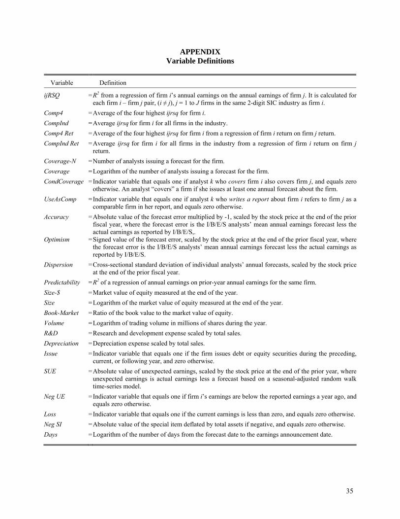
APPENDIX Variable Definitions

 

Variable Definition

ijRSQ = R2 from a regression of firm i’s annual earnings on the annual earnings of firm j. It is calculated for each firm i – firm j pair, (i ≠ j), j = 1 to J firms in the same 2-digit SIC industry as firm i.

Comp4 = Average of the four highest ijrsq for firm i. CompInd = Average ijrsq for firm i for all firms in the industry. Comp4 Ret = Average of the four highest ijrsq for firm i from a regression of firm i return on firm j return. CompInd Ret = Average ijrsq for firm i for all firms in the industry from a regression of firm i return on firm j

return. Coverage-N = Number of analysts issuing a forecast for the firm. Coverage = Logarithm of the number of analysts issuing a forecast for the firm. CondCoverage = Indicator variable that equals one if analyst k who covers firm i also covers firm j, and equals zero

otherwise. An analyst “covers” a firm if she issues at least one annual forecast about the firm. UseAsComp = Indicator variable that equals one if analyst k who writes a report about firm i refers to firm j as a

comparable firm in her report, and equals zero otherwise. Accuracy = Absolute value of the forecast error multiplied by -1, scaled by the stock price at the end of the prior

fiscal year, where the forecast error is the I/B/E/S analysts’ mean annual earnings forecast less theactual earnings as reported by I/B/E/S,.

Optimism = Signed value of the forecast error, scaled by the stock price at the end of the prior fiscal year, wherethe forecast error is the I/B/E/S analysts’ mean annual earnings forecast less the actual earnings asreported by I/B/E/S.

Dispersion = Cross-sectional standard deviation of individual analysts’ annual forecasts, scaled by the stock priceat the end of the prior fiscal year.

Predictability = R2 of a regression of annual earnings on prior-year annual earnings for the same firm. Size-$ = Market value of equity measured at the end of the year. Size = Logarithm of the market value of equity measured at the end of the year. Book-Market = Ratio of the book value to the market value of equity. Volume = Logarithm of trading volume in millions of shares during the year. R&D = Research and development expense scaled by total sales. Depreciation = Depreciation expense scaled by total sales. Issue = Indicator variable that equals one if the firm issues debt or equity securities during the preceding,

current, or following year, and zero otherwise. SUE = Absolute value of unexpected earnings, scaled by the stock price at the end of the prior year, where

unexpected earnings is actual earnings less a forecast based on a seasonal-adjusted random walk time-series model.

Neg UE = Indicator variable that equals one if firm i’s earnings are below the reported earnings a year ago, and equals zero otherwise.

Loss = Indicator variable that equals one if the current earnings is less than zero, and equals zero otherwise.Neg SI = Absolute value of the special item deflated by total assets if negative, and equals zero otherwise. Days = Logarithm of the number of days from the forecast date to the earnings announcement date.

  36

TABLE 1 Descriptive statistics

This table provides descriptive statistics of Comp4, CompInd, and Predictability for the sample before (unrestricted) and after (analyst-restricted) we restrict it to firms with analyst coverage. Panel A presents the mean values of Comp4 and CompInd by year of the observation for the pre- and post-analyst samples. Panel B provides descriptive statistics for the pre-analyst sample. Panel C shows the Pearson correlations for the pre-analyst sample. Variables are defined in the Appendix. Panel A: Average comparability by year for the unrestricted and analyst-restricted samples

Unrestricted Sample Analyst-Restricted Sample Year No. of Obs Comp4 (%) CompInd (%) Obs Comp4 (%) CompInd (%)

1994 2,794 50.3 11.7 1,251 53.7 13.1 1995 2,941 50.9 11.9 1,332 53.8 13.1 1996 3,087 50.4 11.4 1,495 53.0 12.3 1997 3,580 52.2 11.3 1,774 54.1 11.9 1998 3,570 52.1 11.2 1,762 53.8 11.7 1999 3,723 52.2 11.0 1,759 54.0 11.4 2000 3,790 53.3 11.3 1,706 55.6 11.9 2001 3,733 53.5 11.4 1,698 55.7 12.1 2002 3,773 53.9 11.6 1,792 55.9 12.3 2003 3,932 54.5 11.4 1,977 56.8 12.1 2004 3,829 53.9 11.3 2,017 55.9 12.0 2005 3,584 53.6 11.6 1,945 55.0 12.2

Total 42,336 52.7 11.5 20,508 54.9 12.1

Panel B: Descriptive statistics for comparability and predictability for the unrestricted sample

Variable No. of Obs Mean STD 10th Percent Median 90th Percent

Comp4 (%) 42,336 52.7 15.7 32.5 52.4 73.6 CompInd (%) 42,336 11.5 5.4 6.2 10.3 18.3 Predictability (%) 42,336 15.9 21.2 0.2 6.5 47.6

Panel C: Correlations among the comparability and predictability measures for the unrestricted sample

Comp4 CompInd Predictability

Comp4 1.00 0.71 0.24 CompInd 1.00 0.37 Predictability 1.00

  37

TABLE 2 Use of comparable firm in analysts’ reports

This table reports an analysis of the relation between earnings comparability and analysts’ use in their reports of firms in the same industry as the sample firm for the year 2005. The sample includes the combination of analysts reports about sample firms multiplied by the number of firms in each sample-firm’s industry with available data. We estimate various specifications of the following pooled logistic regression:

UseAsCompikj = α + β1 ijRSQij + γ Controlsj + εikj.

Industry fixed effects are included but not tabulated. Coefficient z-statistics are in parentheses. Significance levels are based on one-tailed tests where there is a prediction for the sign of the coefficient and based on two-tailed tests otherwise. ***, ** and * denotes significance at the 1%, 5% and 10% levels, respectively. Variables are defined in the Appendix.

Prediction (1) (2)

ijRSQ + 0.90*** (4.35)

0.76*** (3.62)

Size + 0.27*** (9.12)

0.30*** (7.87)

Volume + 0.22*** (6.67)

0.23*** (6.29)

Book-Market ? 0.11* (1.72)

0.22 (1.58)

ROA ? 0.01 (0.07)

-0.02 (0.03)

Size Difference – -0.42*** (-10.79)

Volume Difference – -0.09*** (-2.42)

Book-Market Difference – -0.32** (-2.06)

ROA Difference – -1.03** (-1.70)

Industry FE Yes Yes

Pseudo R2 3.07% 3.83%

No. of Obs. 39,414 39,414

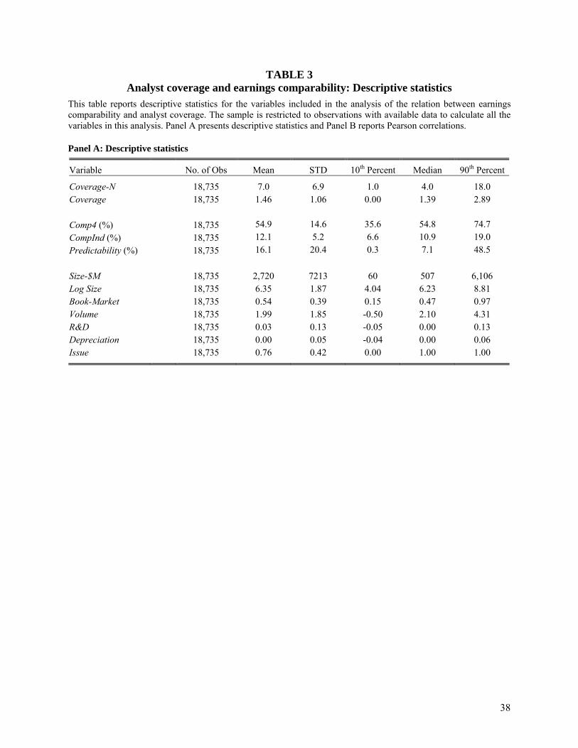
  38

TABLE 3 Analyst coverage and earnings comparability: Descriptive statistics

This table reports descriptive statistics for the variables included in the analysis of the relation between earnings comparability and analyst coverage. The sample is restricted to observations with available data to calculate all the variables in this analysis. Panel A presents descriptive statistics and Panel B reports Pearson correlations. Panel A: Descriptive statistics

Variable No. of Obs Mean STD 10th Percent Median 90th Percent

Coverage-N 18,735 7.0 6.9 1.0 4.0 18.0 Coverage 18,735 1.46 1.06 0.00 1.39 2.89 Comp4 (%) 18,735 54.9 14.6 35.6 54.8 74.7 CompInd (%) 18,735 12.1 5.2 6.6 10.9 19.0 Predictability (%) 18,735 16.1 20.4 0.3 7.1 48.5 Size-$M 18,735 2,720 7213 60 507 6,106 Log Size 18,735 6.35 1.87 4.04 6.23 8.81 Book-Market 18,735 0.54 0.39 0.15 0.47 0.97 Volume 18,735 1.99 1.85 -0.50 2.10 4.31 R&D 18,735 0.03 0.13 -0.05 0.00 0.13 Depreciation 18,735 0.00 0.05 -0.04 0.00 0.06 Issue 18,735 0.76 0.42 0.00 1.00 1.00

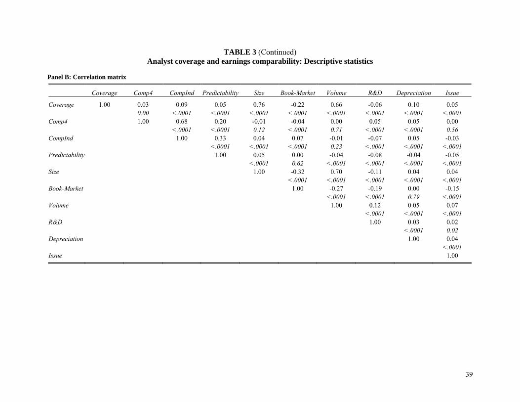
  39

TABLE 3 (Continued) Analyst coverage and earnings comparability: Descriptive statistics

Panel B: Correlation matrix

Coverage Comp4 CompInd Predictability Size Book-Market Volume R&D Depreciation Issue

Coverage 1.00 0.03 0.09 0.05 0.76 -0.22 0.66 -0.06 0.10 0.05 0.00 <.0001 <.0001 <.0001 <.0001 <.0001 <.0001 <.0001 <.0001 Comp4 1.00 0.68 0.20 -0.01 -0.04 0.00 0.05 0.05 0.00 <.0001 <.0001 0.12 <.0001 0.71 <.0001 <.0001 0.56 CompInd 1.00 0.33 0.04 0.07 -0.01 -0.07 0.05 -0.03 <.0001 <.0001 <.0001 0.23 <.0001 <.0001 <.0001 Predictability 1.00 0.05 0.00 -0.04 -0.08 -0.04 -0.05 <.0001 0.62 <.0001 <.0001 <.0001 <.0001 Size 1.00 -0.32 0.70 -0.11 0.04 0.04 <.0001 <.0001 <.0001 <.0001 <.0001 Book-Market 1.00 -0.27 -0.19 0.00 -0.15 <.0001 <.0001 0.79 <.0001 Volume 1.00 0.12 0.05 0.07 <.0001 <.0001 <.0001 R&D 1.00 0.03 0.02 <.0001 0.02 Depreciation 1.00 0.04 <.0001 Issue 1.00

  40

TABLE 4 Analyst coverage and earnings comparability: Multivariate tests

This table reports an analysis of the relation between earnings comparability and analyst coverage. The sample is restricted to observations with available data to calculate all the variables in this analysis. The table reports the results of various specifications of the following regression:

Coverageit+1 = α + β1 Comparabilityit + β2 Predictabilityit + γ Controlsit + εit+1.

Industry and year fixed effects are included for each model but not tabulated. We estimate each model as a panel and cluster the standard errors at the firm level. Coefficient t-statistics are in parentheses. Significance levels are based on one-tailed tests where there is a prediction for the sign of the coefficient and based on two-tailed tests otherwise. ***, ** and * denotes significance at the 1%, 5% and 10% levels, respectively. Variables are defined in the Appendix.

Prediction (1) (2)

Comp4 + 0.23*** (5.15)

CompInd + 0.65*** (5.39)

Predictability + -0.02 -0.02 (-0.50) (-0.70)

Size + 0.32*** 0.32*** (37.66) (37.75)

Book-Market – 0.12*** 0.12*** (5.72) (5.70)

Volume + 0.19*** 0.19*** (23.52) (23.68)

R&D + 0.01 0.01 (0.10) (0.08)

Depreciation + 0.28** 0.27* (1.98) (1.91)

Issue + 0.03* 0.03* (1.89) (1.85)

Industry and Year FE Yes Yes

R2 71.1% 71.1%

No. of Obs. 18,735 18,735

  41

TABLE 5 Analysts’ coverage of comparable firms

This table reports an analysis of the relation between earnings comparability and analyst coverage of firms in the same industry as the sample firm. For each of the years 1994 to 2005 in our sample, we estimate the following logistic regression:

CondCoverageikj = α + β1 ijRSQij + γ Controlsj + εikj.

Industry fixed effects are included but not tabulated. The number of observations used in the annual estimation is the combination of sample firms multiplied by the analysts covering the sample firms multiplied by the number of firms in each sample-firm’s industry with available data. The table presents the mean, maximum, and minimum coefficients, pseudo R2, and number of observations from the 12 annual logistic regressions. Mean coefficient t-statistics (in parentheses) are based on the distribution of the 12 annual coefficients and adjusted for time-series dependence using the Newey-West (1987) correction with one lag. Significance levels are based on one-tailed tests where there is a prediction for the sign of the coefficient and based on two-tailed tests otherwise. ***, **, and * denotes significance at the 1%, 5% and 10% levels, respectively. Variables are defined in the Appendix.

Prediction

Mean (1)

Maximum (2)

Minimum (3)

ijRSQ + 1.01*** (25.41)

1.32 0.78

Size + 0.35*** (11.97)

0.50 0.21

Volume + 0.25*** (25.58)

0.35 0.20

Book-Market – 0.04*** (2.12)

0.15 0.00

R&D + 0.21** (1.97)

0.95 -0.05

Depreciation + 0.62*** (4.33)

1.76 0.02

Issue + 0.01 (0.44)

0.14 -0.15

Industry FE Yes

Pseudo R2 5.97% 9.50% 4.41%

No. of Obs. 2,904,641 4,133,881 1,441,881

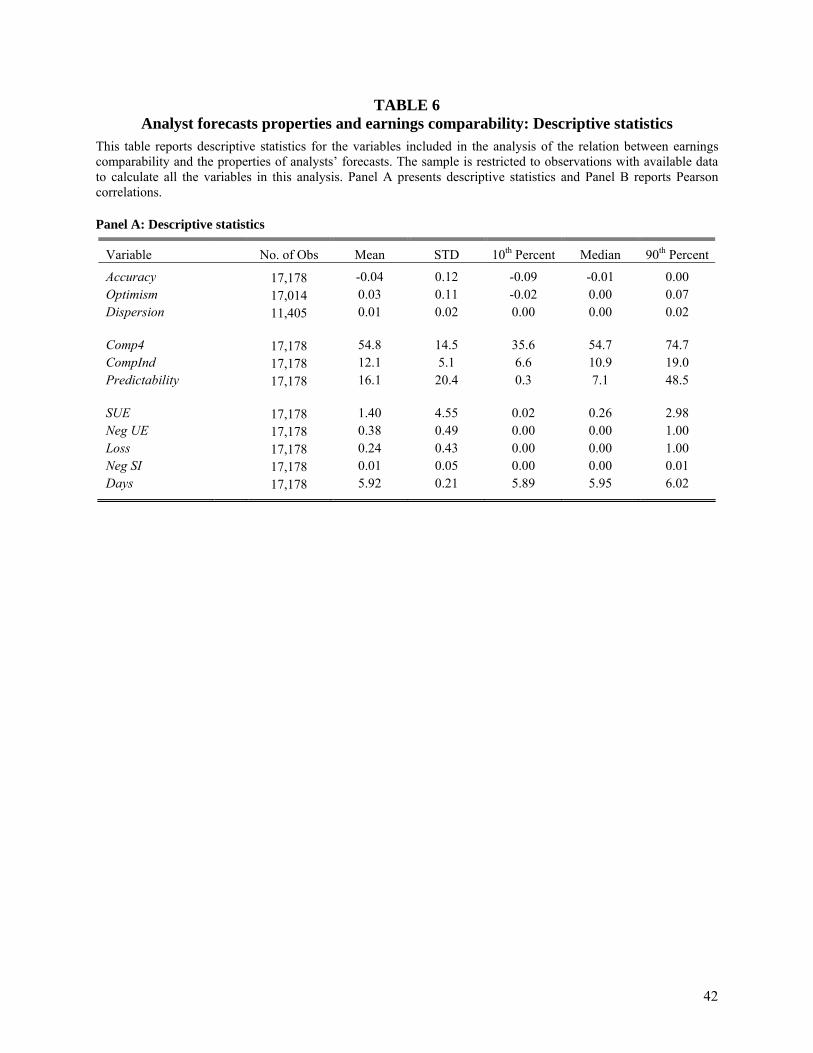
  42

TABLE 6 Analyst forecasts properties and earnings comparability: Descriptive statistics

This table reports descriptive statistics for the variables included in the analysis of the relation between earnings comparability and the properties of analysts’ forecasts. The sample is restricted to observations with available data to calculate all the variables in this analysis. Panel A presents descriptive statistics and Panel B reports Pearson correlations. Panel A: Descriptive statistics

Variable No. of Obs Mean STD 10th Percent Median 90th Percent

Accuracy 17,178 -0.04 0.12 -0.09 -0.01 0.00 Optimism 17,014 0.03 0.11 -0.02 0.00 0.07 Dispersion 11,405 0.01 0.02 0.00 0.00 0.02 Comp4 17,178 54.8 14.5 35.6 54.7 74.7 CompInd 17,178 12.1 5.1 6.6 10.9 19.0 Predictability 17,178 16.1 20.4 0.3 7.1 48.5 SUE 17,178 1.40 4.55 0.02 0.26 2.98 Neg UE 17,178 0.38 0.49 0.00 0.00 1.00 Loss 17,178 0.24 0.43 0.00 0.00 1.00 Neg SI 17,178 0.01 0.05 0.00 0.00 0.01 Days 17,178 5.92 0.21 5.89 5.95 6.02

  43

TABLE 6 (Continued) Analyst forecasts properties and earnings comparability: Descriptive statistics

Panel B: Correlation matrix

Accuracy Optimism Dispersion Comp4 CompInd Predictability SUE Neg UE Loss Neg SI Days

Accuracy 1.00 -0.94 -0.46 0.04 0.03 0.05 -0.06 -0.11 -0.25 -0.06 -0.06 <.0001 <.0001 <.0001 <.0001 <.0001 <.0001 <.0001 <.0001 <.0001 <.0001 Optimism 1.00 0.35 -0.04 -0.04 -0.03 0.02 0.12 0.20 0.05 0.06 <.0001 <.0001 <.0001 0.00 0.00 <.0001 <.0001 <.0001 <.0001 Dispersion 1.00 -0.01 -0.01 -0.09 0.09 0.17 0.38 0.07 0.17 0.25 0.23 <.0001 <.0001 <.0001 <.0001 <.0001 <.0001 Comp4 1.00 0.68 0.20 -0.01 -0.02 0.01 0.01 -0.01 <.0001 <.0001 0.11 0.04 0.50 0.27 0.45 CompInd 1.00 0.33 -0.02 -0.03 -0.06 -0.02 0.03 <.0001 0.03 0.00 <.0001 0.02 <.0001 Predictability 1.00 -0.06 -0.05 -0.08 -0.02 0.02 <.0001 <.0001 <.0001 0.04 0.00 SUE 1.00 0.02 0.15 0.15 0.01 0.02 <.0001 <.0001 0.10 Neg UE 1.00 0.39 0.14 0.03 <.0001 <.0001 0.00 Loss 1.00 0.20 0.05 <.0001 <.0001 Neg SI 1.00 0.02 0.01 Days 1.00

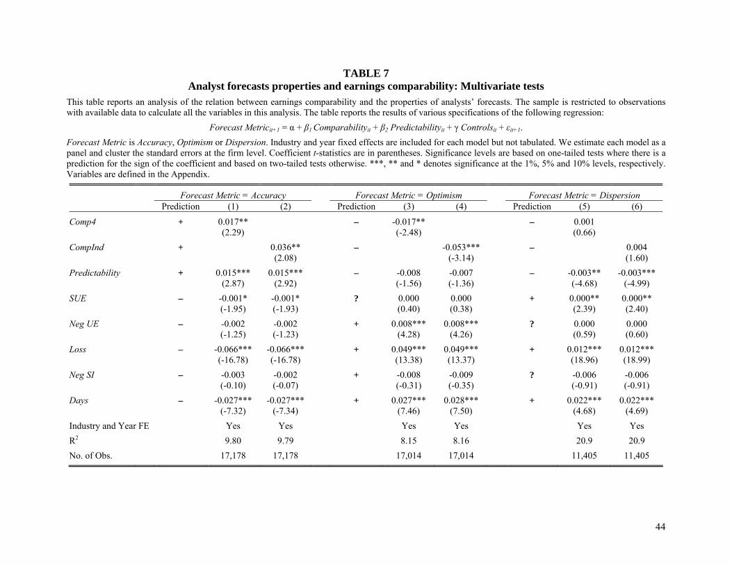
  44

TABLE 7 Analyst forecasts properties and earnings comparability: Multivariate tests

This table reports an analysis of the relation between earnings comparability and the properties of analysts’ forecasts. The sample is restricted to observations with available data to calculate all the variables in this analysis. The table reports the results of various specifications of the following regression:

Forecast Metricit+1 = α + β1 Comparabilityit + β2 Predictabilityit + γ Controlsit + εit+1.

Forecast Metric is Accuracy, Optimism or Dispersion. Industry and year fixed effects are included for each model but not tabulated. We estimate each model as a panel and cluster the standard errors at the firm level. Coefficient t-statistics are in parentheses. Significance levels are based on one-tailed tests where there is a prediction for the sign of the coefficient and based on two-tailed tests otherwise. ***, ** and * denotes significance at the 1%, 5% and 10% levels, respectively. Variables are defined in the Appendix.

Forecast Metric = Accuracy Forecast Metric = Optimism Forecast Metric = Dispersion Prediction (1) (2) Prediction (3) (4) Prediction (5) (6)

Comp4 + 0.017** – -0.017** – 0.001 (2.29) (-2.48) (0.66)

CompInd + 0.036** – -0.053*** – 0.004 (2.08) (-3.14) (1.60)

Predictability + 0.015*** 0.015*** – -0.008 -0.007 – -0.003** -0.003*** (2.87) (2.92) (-1.56) (-1.36) (-4.68) (-4.99)

SUE – -0.001* -0.001* ? 0.000 0.000 + 0.000** 0.000** (-1.95) (-1.93) (0.40) (0.38) (2.39) (2.40)

Neg UE – -0.002 -0.002 + 0.008*** 0.008*** ? 0.000 0.000 (-1.25) (-1.23) (4.28) (4.26) (0.59) (0.60)

Loss – -0.066*** -0.066*** + 0.049*** 0.049*** + 0.012*** 0.012*** (-16.78) (-16.78) (13.38) (13.37) (18.96) (18.99)

Neg SI – -0.003 -0.002 + -0.008 -0.009 ? -0.006 -0.006 (-0.10) (-0.07) (-0.31) (-0.35) (-0.91) (-0.91)

Days – -0.027*** -0.027*** + 0.027*** 0.028*** + 0.022*** 0.022*** (-7.32) (-7.34) (7.46) (7.50) (4.68) (4.69)

Industry and Year FE Yes Yes Yes Yes Yes Yes

R2 9.80 9.79 8.15 8.16 20.9 20.9

No. of Obs. 17,178 17,178 17,014 17,014 11,405 11,405

  45

TABLE 8 Analyst coverage tests: Earnings and return comparability

This table reports an analysis that is identical to that in Table 4 but includes a measure of return comparability. The sample is restricted to observations with available data to calculate all the variables in this analysis. The table reports the results of various specifications of the following regression:

Coverageit+1 = α + β1 Comparabilityit + β2 Predictabilityit + γ Controlsit + εit+1.

Comparability includes measures based on both earnings and return historical covariances. Industry and year fixed effects are included for each model but not tabulated. We estimate each model as a panel and cluster the standard errors at the firm level. Coefficient t-statistics are in parentheses. Significance levels are based on one-tailed tests where there is a prediction for the sign of the coefficient and based on two-tailed tests otherwise. ***, ** and * denotes significance at the 1%, 5% and 10% levels, respectively. Variables are defined in the Appendix.

Prediction (1) (2)

Comp4 + 0.180*** (3.82)

Comp4 Ret + 0.709*** (9.38)

CompInd + 0.503*** (4.09)

CompInd Ret + 1.395*** (6.53)

Predictability + -0.015 -0.013 (-0.15) (-0.37)

Size + 0.311*** 0.326*** (35.80) (36.36)

Book-Market – 0.091*** 0.107*** (4.08) (4.31)

Volume + 0.188*** 0.185*** (21.23) (21.89)

R&D + -0.081 -0.060 (-1.17) (-0.88)

Depreciation + 0.382** 0.375** (2.54) (2.46)

Issue + 0.046** 0.032** (2.44) (2.18)

Industry and Year FE Yes Yes

R2 71.7% 71.7%

No. of Obs. 16,603 16,603

  46

TABLE 9 Analyst forecasts properties tests: Earnings and return comparability

(Table description follows)

Forecast Metric = Accuracy Forecast Metric = Optimism Forecast Metric = Dispersion Prediction (1) (2) Prediction (3) (4) Prediction (5) (6)

Comp4 + 0.013* – -0.012* – 0.001 (1.66) (-1.64) (0.91)

Comp4 Ret + 0.063*** – -0.054*** – 0.001 (6.91) (-6.56) (0.34)

CompInd + 0.031* – -0.042** – 0.004 (1.65) (-2.35) (1.43)

CompInd Ret + 0.172*** – -0.179*** – 0.003 (6.42) (-7.14) (0.78)

Predictability + 0.013** 0.013** – -0.006 -0.005 – -0.003*** -0.003*** (2.24) (2.29) (-1.13) (-1.00) (-4.61) (-4.78)

SUE – 0.000* 0.000 ? 0.000 0.000 + 0.000** 0.000** (-1.64) (-1.54) (0.35) (0.43) (2.01) (2.00)

Neg UE – -0.002 -0.002 + 0.008*** 0.008*** ? 0.000 0.000 (-1.03) (-1.05) (3.97) (4.05) (-0.27) (0.15)

Loss – -0.068*** -0.068*** + 0.050*** 0.051*** + 0.012*** 0.012*** (-15.41) (-15.34) (12.43) (12.50) (17.80) (17.57)

Neg SI – -0.006 -0.001 + -0.011 -0.018 ? -0.005 -0.004 (-0.24) (-0.05) (-0.39) (-0.65) (-0.81) (-0.67)

Days – -0.027*** -0.028*** + 0.029*** 0.029*** + 0.022*** 0.020*** (-6.97) (-7.03) (7.34) (7.35) (4.22) (4.27)

Industry and Year FE Yes Yes Yes Yes Yes Yes

R2 10.13 10.06 8.47 8.53 21.0 20.8

No. of Obs. 15,218 15,218 15,082 15,082 10,238 10,238

  47

TABLE 9 (Continued) Analyst forecasts properties tests: Earnings and return comparability

This table reports an analysis that is identical to that in Table 7 but includes a measure of return comparability. The sample is restricted to observations with available data to calculate all the variables in this analysis. The table reports the results of various specifications of the following regression:

Forecast Metricit+1 = α + β1 Comparabilityit + β2 Predictabilityit + γ Controlsit + εit+1.

Forecast Metric is Accuracy, Optimism or Dispersion. Comparability includes measures based on both earnings and return historical covariances. Industry and year fixed effects are included for each model but not tabulated. We estimate each model as a panel and cluster the standard errors at the firm level. Coefficient t-statistics are in parentheses. Significance levels are based on one-tailed tests where there is a prediction for the sign of the coefficient and based on two-tailed tests otherwise. ***, ** and * denotes significance at the 1%, 5% and 10% levels, respectively. Variables are defined in the Appendix.