THE VALUATION OF CREDIT DEFAULT SWAP OPTIONS

John Hull and Alan White

September, 2002 Revised: January 2003

Joseph L. Rotman School of Management University of Toronto 105 St George Street

Toronto, ON M5S 3E6 Canada

Telephone Hull: 416 978 8615

White: 416 978 3689

e-mail hull@rotman.utoronto.ca

awhite@rotman.utoronto.ca

2

THE VALUATION OF CREDIT DEFAULT SWAP OPTIONS

Abstract

Now that the market for credit default swaps is well established, trading is increasing in

forward credit default swaps and European credit default swap options. This article

develops models for valuing these instruments. The model for valuing European credit

default swap options is very similar to the standard market model for valuing European

swaptions. Once default probabilities and expected recovery rates have been estimated, it

enables traders to calculate option prices from credit default swap spread volatilities and

vice versa. The article concludes by presenting numerical results illustrating the

properties of the models and estimating spread volatilities from historical data.

3

THE VALUATION OF CREDIT DEFAULT SWAP OPTIONS

Credit default swaps (CDSs) have proved to be one of the most successful financial

innovations of the 1990s. They are instruments that provide insurance against a particular

company (or sovereign entity) defaulting on its debt. The company is known as the

reference entity and a default by the company is known as a credit event. The buyer of

the protection makes periodic payments to the seller of protection at a predetermined

fixed rate per year. The payments continue until the end of the life of the contract or until

a credit event, whichever is earlier. If a credit event occurs, the buyer of protection has

the right to deliver a bond issued by the reference entity (the reference bond) to the seller

of protection in exchange for its face value.

The amount of the payments made per year by the buyer is known as the CDS spread.

Suppose, for example, that the CDS spread for a five-year contract on Ford Motor Credit

with a principal of $10 million is 200 basis points. This means that the buyer can enter

into a five-year contract where $200,000 per year is paid and the right to sell bonds

issued by Ford with a face value of $10 million for $10 million in the event of a default

by Ford during the life of the CDS is obtained.

In a standard contract, payments are made semiannually or quarterly in arrears. If the

reference entity defaults, there is a final accrual payment covering the period from the

previous payment to the default date and payments then stop. Contracts are sometimes

settled in cash rather than by the delivery of bonds. In this case there is a calculation

agent who has the responsibility of determining the market price of bonds issued by the

4

reference entity a specified number of days after the credit event. The cash settlement is

then the face value of the bond less the post-default market price.

As we show in Hull and White (2000) the valuation of a CDS requires estimates of the

recovery rate and the probability of default in a risk-neutral world. Once the recovery rate

has been estimated the probability of default can be calculated from the prices of bonds

issued by the reference entity or from the spreads quoted for other CDSs on the reference

entity. The pricing of a vanilla CDS is relatively insensitive to the recovery rate providing

the same recovery rate is used to estimate default probabilities and to value the CDS. As

shown in Hull et al (2002), when bond prices are used to calculate default probabilities

the benchmark risk-free rate should be assumed to be the swap rate or slightly below the

swap rate.

Now that the market for CDSs is well established, a market is developing in forward

CDSs and CDS options. A forward CDS contract is the obligation to buy or sell a CDS

on a specified reference entity for a specified spread at a specified future time. For

example, a particular forward contract might obligate the holder to buy five-year

protection on Ford Motor Credit starting in one year for 200 basis points per year. The

forward CDS ceases to exist if the reference entity (Ford in this case) defaults during teh

life(1 year in this case) of the forward contract. We define the forward CDS spread as the

specified spread that causes the forward contract to have a value of zero.

A CDS option is defined analogously to a forward credit default swap. It is a European

option that gives the holder the right to buy or sell protection on a specified reference

entity for a specified future period of time for a certain spread. The option is knocked out

if the reference entity defaults during the life of the option. For example, a call CDS

5

option might allow the holder to buy protection on Ford Motor Credit for five years

starting in one year for 200 basis points per year. If Ford defaults during the one-year life

of the option, the option is knocked out. If Ford does not default during this period, the

option will be exercised if the market price of five-year protection on Ford is greater than

200 basis points at the end of the life of the option.

In this article we examine how a forward CDS and a CDS option can be priced.

Assuming that a full term structure of CDS spreads is known, the valuation of a forward

CDS depends on one unobservable variable, the expected recovery rate. A CDS option

depends on two unobservable variables: the expected recovery rate and the volatility. We

examine the role played by these unobservable variables in the pricing. We also present

some historical data on the volatility of CDS spreads for companies with different credit

ratings.

I. Valuation of CDS and Forward CDS

In this section we consider a CDS that gives the holder the obligation to buy protection

on a particular reference entity between times T and T* for a spread of K per annum when

the notional principal is L. When T = 0 this is a regular CDS. When 0 < T < T* it is a

forward CDS.

Let q(t)δt be the risk-neutral probability of default between time t and t + δt as seen at

time zero.1 The probability that the company will survive to time t is then

π τ ττ

( ) ( )t q dt

= −=∫1

0

1 Note that this is not the hazard rate. The hazard rate, h(t), is defined so that h(t)δt is the probability of default between times t and t + δt conditional on no earlier default.

6

We also define:

u(t): The present value of payments at the rate of $1 per year on the payment dates of

the underlying CDS between times T and t (T < t ≤ T*)

e(t): The present value of the final accrual payment that would be required on the CDS

at time t in the event of a default at time t if payments were made at the rate of $1

per year2

v(t): The present value of $1 received at time t

A(t): The accrual interest on the reference bond at time t as a percent of face value

R̂ : The expected risk-neutral recovery rate on the reference bond defined as a

percentage of the claim amount. The claim amount is assumed to be the face value

of the bond plus accrued interest.3

The valuation of a forward CDS is analogous to the valuation of a regular CDS described

in Hull and White (2000). We compute the expected present value of payments and

benefits of the swap, taking expectations over default events. As in Hull and White

(2000) we make the assumption that default events, interest rates, and recovery rates are

mutually independent.

If there is a credit event prior to time T the payments and benefits are zero. If a default

occurs at time t (T < t < T*), the present value of the payments is LK [u(t)+e(t)]. If there

is no default prior to time T*, the present value of the payments is LK u(T*). The

expected present value of the payments is therefore

2 The accrual payment is approximately t – t* where t* is the payment date immediately preceding time t

7

[ ]{ }LK q t u t e t dt T u Tt T

T( ) ( ) ( ) ( *) ( *)

*+ +

=∫ π (1)

The recovery made on the reference bond in the event of a default at time t (T < t < T*) is

( ) ˆ1L A t R+

so that the payoff from the CDS if there is a default at time t (T < t < T*) is

( ) ˆ1L L A t R− +

The present value of the expected payoff from the CDS is therefore

( ) ( ) ( )* ˆ ˆ1

T

t TL R A t R q t v t dt

= − − ∫ (2)

The value of the forward CDS to the buyer of protection is the present value of the

expected benefit minus the present value of the expected payments the buyer will make.

From equations (1) and (2) this is

[ ] [ ]{ }∫ ∫=

= =π++−−−

* **)(*)()()()()()(ˆ)(ˆ1

Tt

Tt

T

TtTuTdttetutqLKdttvtqRtARL (3)

The forward CDS spread, which we will denote by F, is the value of K that makes this

expression zero:

[ ][ ]

FR A t R q t v t dt

q t u t e t dt T u Tt T

T

t T

T=− −

+ +

=

=

∫∫

1 $ ( ) $ ( ) ( )

( ) ( ) ( ) ( *) ( *)

*

*π

(4)

3 For convenience, analysts often define the recovery rate as a percentage of the face value of the bond. (The recovery rate is then slightly dependent on the bond's coupon.) Our valuation equations are correct for

8

Setting T = 0 and we get the formula in Hull and White (2000) for the spot CDS spread,

S, applicable to a contract maturing at time T*:

[ ][ ]

SR A t R q t v t dt

q t u t e t dt T u Tt

T

t

T=− −

+ +

=

=

∫∫

10

0

$ ( ) $ ( ) ( )

( ) ( ) ( ) ( *) ( *)

*

*π

(5)

The usual practice when applying equations (3), (4) or (5) is to assume that A(t) = 0. (See

footnote 3.) The assumption is convenient because the valuation then requires no

information about the reference bond. In many situations it is also a defensible

assumption because there are often a number of bonds that can be delivered in the event

of a default and the buyer of protection will find that the cheapest-to-deliver bond is the

one for which the accrued interest is least.

Some assumption must be made about the nature of the probability density function q(t).

In Hull and White (2000) we assume that q(t) is a step function so that

iii tttqtq <≤= −1 when )(

for some qi (1 ≤ i ≤ n) where t0 < t1 < t2....< tn. Communications from J.P. Morgan (who

have been a leader in developing credit derivatives markets) indicate that the market

practice is slightly different from this. The hazard rate, h(t), rather than the default

probability density q(t) is usually assumed to be a step function. This does have one

important practical advantage: the cumulative probability of default, however far ahead

one looks is never greater than 1. Suppose that the hazard rate is hi between ti-1 and ti.

Because

∫=ττ−

tdh

ethtq 0)(

)()(

this definition if we set A(t) = 0

9

it follows that

−−−−= ∑

−

=−−

1

111 )()(exp)(

i

jjjjiii tthtthhtq

for ti-1 ≤ t < ti.

A final point is that the expression for the present value of the payments can also be

written in terms of the survival probabilities. Suppose that the payments by the CDS

buyer are due to be made at times ti (i = 1, 2, ...n). The probability of the ith payment

being made is π(ti). Setting ∆i = ti - ti-1, an expression that is equivalent to equation (1) for

the present value of the payments

+∆π∑ ∫= =

n

i

T

Ttiii dttetqtvtLK

1

*

)()()()(

When the assumption A(t) = 0 is made, the expression for the CDS value in equations (3)

is equivalent to

∫ ∫∑= ==

+∆π−−* *

1)()()()()()()ˆ1(

T

Tt

T

Tt

n

iiii dttetqtvtLKdttvtqRL

and equations (4) and (5) are equivalent to

∫∑

∫

==

=

+∆π

−=

*

1

*

)()()()(

)()()ˆ1(

T

Tt

n

iiii

T

Tt

dttetqtvt

dttvtqRF

∫∑∫

==

=

+∆π

−=

*

01

*

0

)()()()(

)()()ˆ1(T

t

n

iiii

T

t

dttetqtvt

dttvtqRS

10

II. Valuation of CDS Options

It is natural to try to value a CDS option by using an approach similar to that of

Jamshidian (1997) for valuing a European swaption. We first review Jamshidian’s

argument and then consider how it can be applied to CDS options.

Jamshidian’s Argument for European Swaptions

The forward swap rate, R, for a vanilla swap is the ratio of the prices of two traded

securities:

gfR =

where f is the present value of the floating cash flows on the underlying swap when the

notional principal is $1 and g is the present value of fixed cash flows on the underlying

swap at the rate of $1 per year. Jamshidian uses g as the numeraire security for valuing

the European swap option. There is a probability measure M under which all security

prices are martingales when g is the numeraire. Under this probability measure R is a

martingale so that for a forward start swap starting at T

R E SM T0 = ( ) (6)

where R0 is the value of R at time zero, ST is the swap rate realized at time T, and EM

denotes expectation under the measure.

Define V as the value of a European option on a swap lasting between times T and T* in

which we receive a fixed rate of K on a notional principal of $1. The variable gV is the

ratio of two traded securities and is a martingale under the probability measure M. This

means that

11

=

T

TM g

VE

gV

0

0 (7)

where V0 and g0 are the values of V and g at time zero, and VT and gT are their values at

time T.

Because VT = gT max(ST −K, 0), equation (7) implies

( )0 0 max ,0M TV g E S K= − (8)

Using the result in equation (6) and assuming that ln ST is normal with standard deviation

TSσ we obtain the formula for valuing the European swap option

( ) ( )0 0 0 1 2V g R N d KN d= − (9)

where N is the cumulative normal distribution function and

( ) 20

1 2 1

ln / / 2;S

SS

R K Td d d T

T+σ

= = −σσ

Extension to CDS Options

Consider next a call option on a CDS with a notional principal of $1 in which we have

the right to buy protection on a particular reference entity between times T and T* for a

spread of K. We redefine variables as follows:

f: The present value of the payoff on the CDS for a notional principal of $1.

g: The present value of payments on the CDS at the rate of $1 per year.

ST: The realized CDS spread at time T

12

V: The value of CDS option

From equation (4) the forward CDS spread, F, is the ratio of two security prices:

fFg

=

It appears that Jamshidian’s argument in equations (6), (7), (8), and (9) can be used with

our redefined variables and R replaced by F. However there is a problem. If the reference

entity defaults at a time t between time 0 and time T, f = g = 0 between times t and T, and

F is undefined during this period.

Luckily we can overcome this problem by considering all variables and security prices in

a world conditional on no default by the reference entity prior to time T. Schonbucher

(2000) provides a formal proof of the validity of this approach. Define

f*: The present value of the payoff on the CDS for a notional principal of $1

conditional on no default by reference entity prior to time T

g*: The present value of payments at the rate of $1 per year on the CDS conditional on

no default by reference entity prior to time T

g0*: Value of g* at time zero

V0*: The value of the CDS option at time zero conditional on no default by reference

entity prior to time T

The forward CDS spread is given by

**

gfF =

13

This is always well defined in the world we are considering. Using g* as the numeraire

security, we assume that, conditional on no default prior to time T, ST is lognormal with

the standard deviation of ln ST being Tσ . An argument analogous to that given above

for European swap options shows that the value of the option condition on no default

prior to time T is given by

( ) ( )0 0 0 1 2* *V g F N d KN d= −

where

( ) 20

1 2 1

ln / / 2;

F K Td d d T

T+σ

= = −σσ

The probability of no default prior to time T is π(T) so that

g0 = π(T) g0* and V0 = π(T) V0*

It follows that4

( ) ( )0 0 0 1 2V g F N d KN d= −

or substituting for g0

[ ] [ ]V F N d KN d q t u t e t dt T u Tt T

T

0 0 1 2= − + +=∫( ) ( ) ( ) ( ) ( ) ( *) ( *)

*π (10)

or alternatively

[ ]

+∆π−= ∫∑ ==

*

12100 )()()()()()(

T

Tt

n

iiii dttetqtvtdKNdNFV (11)

4 This formula was also produced independently by Schonbucher (2000)

14

Because the notional principal is $1, equations (10) and (11) give the option price in the

units in which the forward CDS rate is specified. We refer to σ as the CDS spread

volatility. As the market for CDS options becomes established it is likely that that

implied volatilities for CDS options will be produced in much the same way that implied

volatilities are produced for options on other assets.

III. Numerical Example

We now present a numerical example to illustrate the application of equations (4) and

(10) and test the sensitivity of results to assumptions.

In Hull and White (2000) we showed how default probabilities can be estimated from the

yields on corporate bonds. Now that the CDS market is well established an alternative

approach is to imply default probabilities from quoted CDS spreads. This is discussed in

Hull (2003, p. 641). It is more appealing to participants in the CDS options market

because it relates the prices of CDS options directly to quotes on the underlying. It also

avoids the need to choose a benchmark risk-free rate.5 It is the approach we will use here.

Suppose that the zero-coupon yield curve is flat at 5% (continuously compounded) and

CDS spreads for a particular reference entity are as shown in Table 1. We consider a

CDS where payments are made quarterly. In our base case:

1. The recovery rate is 40%

2. A(t) = 0. (See footnote 3)

3. The probability density function, q(t), is a step function of the form:

5 Hull et al's (2002) research suggests that the benchmark risk-free rate is about 10 basis points below the swap rate

15

( )

1

2

3

4

5

0 11 22 33 55 10

q tq t

q t q tq tq t

≤ < ≤ <= ≤ < ≤ <

≤ <

Reverse engineering the formula for the spot CDS spread in equation (5) gives the values

for q(t) in Table 2.

Define an m×n forward (option) contract as the obligation (right) in m year’s time to enter

into CDS lasting n years. Table 3 shows 1×1, 1×2, 1×3, 1×5, 3×1, 3×2, 3×3, 3×5, 5×1,

5×2, 5×3, 5×5, forward CDS spreads and call option prices calculated using equations (4)

and (10). The strike spreads for the options are shown in the table. In all cases the spread

volatilities were assumed to be 40% per annum. Table 3 also shows that option prices

increase as both the maturity of the option and the life of the underlying CDS increase.

As the maturity of the option increases the volatility is applied for a longer time period;

as the life of the underlying CDS increases the payoff consists of more cash flows.

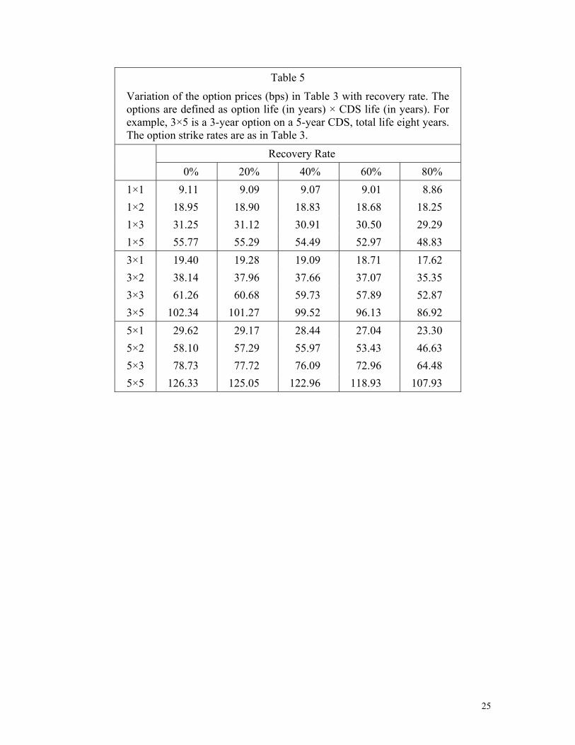
A key assumption in producing the numbers in Table 3 is the recovery rate. Tables 4 and

5 show how the forward rates and option prices in Table 3 change as the recovery rate

changes from 0% to 80% for our base case. Even extreme changes in the recovery rate

assumption make very little difference to the forward CDS spread. This is similar to the

result we obtained in Hull and White (2000) for spot CDS spreads. As the recovery rate

increases, the probabilities of default that are calculated from the CDS spreads in Table 1

increase. However, when the payoff from a forward CDS spread is calculated the higher

default probabilities almost perfectly offset by the higher recovery rates.

16

Table 5 shows the sensitivity of the prices of the options we are considering to the

recovery rate is also quite low. The percentage impact of the recovery rate increases as

the life of the option increases and as the life of the underlying CDS increases, but is

never very large. A change in the recovery rate from 20% to 60% reduces the option

price by less than 10%. It appears that we do not need precise estimates of the recovery

rate to obtain reasonable option prices.6

One assumption we make in producing Tables 2 to 5 is that the default probability

density function, q(t), is a step function. An alternative assumption is that q(t) is a

continuous piecewise linear (PWL) function. That is,

( )( )

( )( )

( )

1

1 2

1 2 3

1 2 3 4

1 2 3 4 5

0 11 1 2

2 2 33 3 5

2 5 5 10

q tq s t tq s s t tq tq s s s t tq s s s s t t

≤ < + − ≤ < + + − ≤ <= + + + − ≤ <

+ + + + − ≤ <

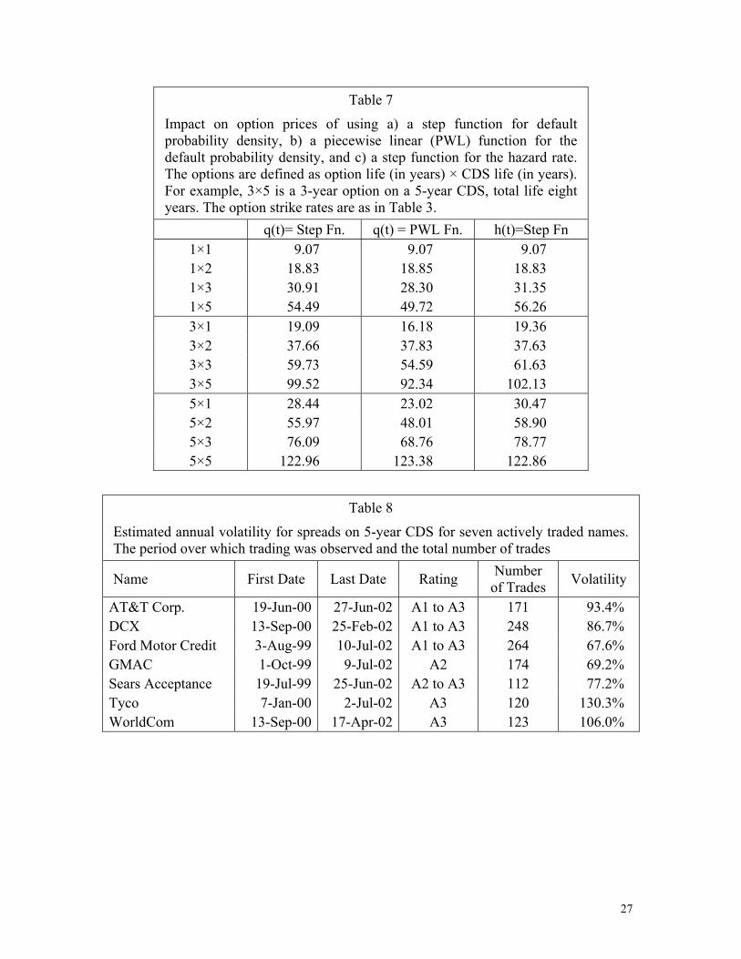
Figure 1 compares the two functions for our base case. Tables 6 and 7 compare the

results of the step function model, the PWL model, and the model where it is the hazard

rate rather than the default probability density that is a step function

The three models give very similar results for 1×1 and 1×2 forward prices and 1×1 and

1×2 option prices. They produce different results for the 1×3 forward CDS rates and 1×3

CDS options because they disagree about the risk-neutral probability of a default during

the fourth year. Under the step model this probability is about 1.33%; under the PWL

model it is about 1.24% ; and under the hazard-rate step model it is about 1.34%.

6 In one sense this is unfortunate. Quoted option prices will not be useful in helping us simultaneously estimate default probabilities and recovery rates.

17

Similarly they produce different results for the 1×5 forward CDS rates and 1×5 CDS

options because they disagree about the probability of a default during the sixth year.

Under the step model this probability is about 1.76%; under the PWL model it is about

1.58%; and under the hazard-rate step model it is about 1.82%. The variation in the

forward CDS spreads and option prices across the models for the other options

considered can be explained similarly.

The examples considered so far have assumed that the recovery rate is defined as in

footnote 3. We tested the effect of assuming a ten-year reference bond with a coupon of

5% when carrying out all calculations. The recovery rate was kept the same. Default

probabilities increased while payoffs decreased. The overall effect on both forward CDS

spreads and option prices was very small. The average absolute error for the forward

spreads was 0.36 of a basis point; the average absolute error for the option prices was

0.46 of a basis point. This provides some justification for the market’s practice of setting

A(t) = 0.

IV. Historical Volatilities

In our example in the previous section we assumed that the CDS spread volatility was

40%. To determine whether this is a reasonable value we estimated some historical

realized volatilities from CDS spread quotes provided to us by GFI, a broker specializing

in CDS trading. The data covers the period from January 5, 1998 to May 24, 2002 and

contains over 200,000 individual quotes. Each quote contains the following information:

1. The date on which the quote was made,

2. The name of the entity underlying the CDS,

18

3. The life of the CDS,

4. Whether the quote is a Bid (wanting to buy protection) or an Offer (wanting to sell

protection), and

5. The CDS quote in basis points.

Each quote is a firm quote for a minimum notional of 10 million USD.7

The quotes in the database may be bids, or offers, or bids and offers. When the broker

registers a transaction, the bid and offer are the same. To simplify the calculation of

historical volatilities we focused on actual transaction prices. Because the CDS spreads

vary with contract maturity we considered only 5-year CDS transactions. (Five years is

by far the most popular CDS life.)

The volatility was computed much in the same way as one would compute stock price

volatility. First we compute the trade-to-trade return for the i’th trade, Ri = ln (Si / Si–1)

and the time between trades, ∆i = ti – ti–1 where Si is the i’th spread and ti is the time at

which the i’th spread is observed. The standard deviation of these returns, s, and the mean

of the time intervals, m, are then computed.

( ) [ ]

( ) nm

nnRRns

n

i i

n

i

n

i ii

/

)1(/

1

1

2

12

∑

∑ ∑

=

= =

∆=

−

−=

The volatility estimate is then

ˆ sm

σ =

19

Table 8 shows volatilities for the seven names that provided the greatest number of

reported trades during the period covered by our data. These ranged from 67.6% per

annum for Ford Motor Credit to 130.3% per annum for Tyco. All the companies were A-

rated during the period covered by the observations, but in some cases the rating changed

between A1 (the best A rating) and A3 (the worst A rating). In all cases of ratings

change, the changes were downgrades, never upgrades.

For comparison purposes we also computed the volatility of the average spread level for

three different rating classes, Aaa- and Aa-rated, A-rated, and Baa-rated. The first two

categories are grouped together because the number of CDS quotes for Aaa-rated entities

is very small. The average spread level is represented by an index we constructed of

quoted CDS spreads. For the three indices the volatilities computed over the same

interval (August 30, 2000 to June 24, 2002) are: Aaa/Aa = 69.0%, A = 48.7%, and Baa =

52.2%.

To put some perspective on these relatively high volatilities suppose that successive

proportional changes in the CDS spread were independent. In this case future CDS

spreads are drawn from a lognormal distribution. If the CDS spread were 100 basis points

today and the volatility were 60.0%, the 95% confidence interval for the CDS spread in 1

year’s time would be between 31 and 324 basis points. This large range seems at odds

with the observed behavior of CDS spreads, which suggests that the sequential

independence assumption is probably not correct. It is more likely that CDS spreads

7 The vast majority of the quotations are for CDS denominated in USD. However, there is increasing activity in EUR and JPY. The proportion of the quotes denominated in USD from 1998 to 2002 is: 100%, 99.9%, 97.7%, 92.2%, and 71.4%.

20

behave like interest rates and exhibit some sort of mean-reverting behavior. This means

that when we are pricing options on CDS spreads these volatilities are only appropriate

for relatively short term options. For longer term options the mean reversion will lower

the volatility appropriate for equation (10).

V. Conclusions

The market for CDS swaps has grown very fast in the last five years and a market is now

developing in CDS options. Many market participants argue that a necessary condition

for an active options market is a standard market model enabling them to calculate a

volatility from a price or a price from a volatility. In this paper we have suggested a

candidate for the standard market model in the CDS options market. The main

assumption of the model is that the CDS spread at a future time conditional on no earlier

default is lognormal.

The pricing formula given by the model for European CDS options is very similar to that

given by the standard market model for European swap options. One complication is that

it involves two unobservable parameters: the expected recovery rate and the volatility.

However, the option prices are only weakly dependent on the recovery rate and it is likely

that most traders will be comfortable keeping the recovery rate parameter fixed at a pre-

agreed level when quoting volatilities.

Our sensitivity analysis shows that option prices can be quite sensitive to the assumptions

made about the default probability distribution. When quotes for only a handful of

maturities are available many different reasonable default probability distributions can be

fitted to them. The stepwise hazard rate model may well emerge as the market standard

for converting prices into volatilities and vice versa. However, it is likely to be important

21

for market participants to experiment with alternative assumptions about the nature of the

default probability distribution.

The valuation of CDS options requires quotes on CDS spreads to be available for a

variety of different maturities. Unfortunately the vast majority of the trading in CDSs is

in instruments with five-year maturities. The simplest assumption for the purpose of

quoting volatilities is that all CDS spreads equal the five-year CDS spread. A slightly less

restrictive assumption is to assume that the CDS spread is a linear function of maturity

and estimate the slope for a rating category from the non-five-year data that is available.

A more sophisticated assumption might be that the excess of the n-year CDS spread over

the n-year bond yield spread for a reference entity is the same as the excess of the five-

year CDS spread over the five-year bond yield spread.

22

References

Hull, J. C., Options, Futures, and Other Derivatives, Prentice Hall, Englewood Cliffs, NJ

2003.

Hull, J.C., M. Predescu-Vasvari and A. White, “The relationship between credit default

swap spreads, bond yields and credit rating announcements,” Working Paper, University

of Toronto, 2002.

Hull, J. C. and A. White, “Valuing credit default swaps I: No counterparty default risk,”

Journal of Derivatives, vol. 8, no. 1 (Fall 2000), pp 29-40.

Jamshidian F., “LIBOR and swap market models and measures” Finance and Stochastics,

1, 4 (1997), pp 293-330.

Schonbucher, P. J., “A LIBOR market model with default risk,” Working paper,

University of Bonn, Department of Statistics, 2000.

23

Table 1

CDS quotes for a typical A-rated entity. The CDS payments are made quarterly in arrears.

CDS Maturity (Years)

CDS Rate (Basis points per year)

1 54

2 58

3 62

5 70

10 90

Table 2

Stepwise default probability density function, q(t) and cumulative density inferred from CDS spreads in Table 1. A recovery rate of 40% is assumed.

T q(t) T q t dtt

T( )

=∫ 0

0 ≤ t < 1 0.00890 1 0.00890 1 ≤ t < 2 0.01017 2 0.01907 2 ≤ t < 3 0.01141 3 0.03048 3 ≤ t < 5 0.01327 5 0.05703 5 ≤ t < 10 0.01756 10 0.14481

24

Table 3

Forward CDS spreads and option prices calculated from the data in Table 2. Recovery rate = 40% and CDS spread volatility = 40%.

CDS Start (Years)

CDS Life(Years)

Forward CDS Spread (bps)

Option Strike Price (bps)

Option Price (bps)

1 1 62.25 62.00 9.07 1 2 66.36 66.00 18.83 1 3 71.59 70.00 30.91 1 5 81.45 80.00 54.49 3 1 83.22 80.00 19.09 3 2 83.87 80.00 37.66 3 3 93.12 90.00 59.73 3 5 101.65 100.00 99.52 5 1 113.45 110.00 28.44 5 2 114.50 110.00 55.97 5 3 115.55 120.00 76.09 5 5 117.65 120.00 122.96

Table 4

Variation of the forward CDS spreads (bps) in Table 3 with recovery rate. Contracts are defined as life of forward (in years) × CDS life (in years). For example, 3×5 is a 3-year forward on a 5-year CDS, total life eight years.

Recovery Rate

0% 20% 40% 60% 80% 1×1 62.23 62.24 62.25 62.27 62.33 1×2 66.33 66.34 66.36 66.39 66.50 1×3 71.61 71.61 71.59 71.57 71.52 1×5 81.63 81.56 81.45 81.23 80.65 3×1 83.26 83.24 83.22 83.18 83.07 3×2 83.68 83.75 83.87 84.11 84.82 3×3 93.31 93.24 93.12 92.91 92.38 3×5 101.69 101.67 101.65 101.62 101.62 5×1 114.25 113.95 113.45 112.48 109.81 5×2 114.89 114.74 114.50 114.04 112.81 5×3 115.52 115.53 115.55 115.61 115.92 5×5 116.77 117.10 117.65 118.79 122.51

25

Table 5

Variation of the option prices (bps) in Table 3 with recovery rate. The options are defined as option life (in years) × CDS life (in years). For example, 3×5 is a 3-year option on a 5-year CDS, total life eight years. The option strike rates are as in Table 3.

Recovery Rate

0% 20% 40% 60% 80% 1×1 9.11 9.09 9.07 9.01 8.86 1×2 18.95 18.90 18.83 18.68 18.25 1×3 31.25 31.12 30.91 30.50 29.29 1×5 55.77 55.29 54.49 52.97 48.83 3×1 19.40 19.28 19.09 18.71 17.62 3×2 38.14 37.96 37.66 37.07 35.35 3×3 61.26 60.68 59.73 57.89 52.87 3×5 102.34 101.27 99.52 96.13 86.92 5×1 29.62 29.17 28.44 27.04 23.30 5×2 58.10 57.29 55.97 53.43 46.63 5×3 78.73 77.72 76.09 72.96 64.48 5×5 126.33 125.05 122.96 118.93 107.93

26

Table 6

Impact on forward CDS spreads of using a) a step function for default probability density, b) a piecewise linear (PWL) function for the default probability density, and c) a step function for the hazard rate. Contracts are defined as life of forward (in years) × CDS life (in years). For example, 3×5 is a 3-year forward on a 5-year CDS, total life eight years.

q(t) = Step Fn. q(t) = PWL Fn. h(t)=Step Fn 1×1 62.25 62.24 62.25 1×2 66.36 66.37 66.36 1×3 71.59 69.86 71.75 1×5 81.45 79.41 82.18 3×1 83.22 77.52 83.74 3×2 83.87 84.02 83.84 3×3 93.12 89.57 94.41 3×5 101.65 98.40 102.81 5×1 113.45 101.82 117.64 5×2 114.50 105.75 117.64 5×3 115.55 109.71 117.64 5×5 117.65 117.76 117.64

27

Table 7

Impact on option prices of using a) a step function for default probability density, b) a piecewise linear (PWL) function for the default probability density, and c) a step function for the hazard rate. The options are defined as option life (in years) × CDS life (in years). For example, 3×5 is a 3-year option on a 5-year CDS, total life eight years. The option strike rates are as in Table 3.

q(t)= Step Fn. q(t) = PWL Fn. h(t)=Step Fn 1×1 9.07 9.07 9.07 1×2 18.83 18.85 18.83 1×3 30.91 28.30 31.35 1×5 54.49 49.72 56.26 3×1 19.09 16.18 19.36 3×2 37.66 37.83 37.63 3×3 59.73 54.59 61.63 3×5 99.52 92.34 102.13 5×1 28.44 23.02 30.47 5×2 55.97 48.01 58.90 5×3 76.09 68.76 78.77 5×5 122.96 123.38 122.86

Table 8

Estimated annual volatility for spreads on 5-year CDS for seven actively traded names. The period over which trading was observed and the total number of trades

Name First Date Last Date Rating Number of Trades Volatility

AT&T Corp. 19-Jun-00 27-Jun-02 A1 to A3 171 93.4% DCX 13-Sep-00 25-Feb-02 A1 to A3 248 86.7% Ford Motor Credit 3-Aug-99 10-Jul-02 A1 to A3 264 67.6% GMAC 1-Oct-99 9-Jul-02 A2 174 69.2% Sears Acceptance 19-Jul-99 25-Jun-02 A2 to A3 112 77.2% Tyco 7-Jan-00 2-Jul-02 A3 120 130.3% WorldCom 13-Sep-00 17-Apr-02 A3 123 106.0%

28

Figure 1

Default Probability Density Functions

0.00000

0.00500

0.01000

0.01500

0.02000

0.02500

0 1 2 3 4 5 6 7 8 9 10

Time (Years)

StepPWL