Embed Size (px)
Citation preview
RA
FAEL R
AVN
IK AN
D IVAN ŽILIĆ:
THE U
SE OF SVA
R AN
ALY
SIS IN DETER
MIN
ING TH
E EFFECTS O
F FISCA
L SHO
CK
S IN CR
OATIA
FINA
NC
IAL TH
EORY A
ND
PRA
CTIC
E35 (1) 25-58 (2011)
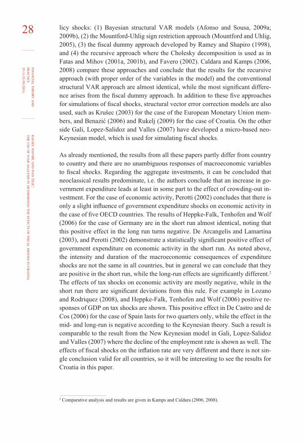
25The use of SVAR analysis in determining the effects of fiscal shocks in CroatiaRAFAEL RAVNIK*
Croatian National Bank, [email protected]
IVAN ŽILIĆ*
Article**
JEL: E62, H30, H150
UDC: 336.1
* The authors thank the two anonymous referees for their insight, helpful comments and suggestions. Also, authors would like to thank prof. dr. sc. Ivo Bićanić for motivation, support and overall efforts. The views expressed in this paper are those of the authors alone and any of the remaining errors is the authors’ responsibility.
** Received: June 1, 2010 Accepted: November 16, 2010

RA
FAEL R
AVN
IK AN
D IVAN ŽILIĆ:
THE U
SE OF SVA
R AN
ALY
SIS IN DETER
MIN
ING TH
E EFFECTS O
F FISCA
L SHO
CK
S IN CR
OATIA
FINA
NC
IAL TH
EORY A
ND
PRA
CTIC
E35 (1) 25-58 (2011)
26 AbstractIn this paper we use multivariate Blanchard-Perotti SVAR methodology to analyze disaggregated short-term effects of fi scal policy on economic activity, infl ation and short-term interest rates. The results suggest that the effects of government expenditure shocks and the shock of government revenues are relatively the hi-ghest on interest rates and the lowest on infl ation. A tax shock in the short term increases the infl ation rate and also decreases the short-term interest rate, and after one year stabilization occurs at the initial level, while spending shock leads to a reverse effect. The effects of fi scal policies on the proxy variable of output, i.e. industrial production, are less economically intuitive, because the shock of expenditure decreases and revenue shock permanently increases industrial pro-duction. The empirical result shows that a tax shock has a permanent effect on future taxes; while future levels of government spending are not related to current expenditure shocks. Interactions between the components of fi scal policy are also examined and it is concluded that a tax shock increases expenditures permane-ntly, while an expenditure shock does not signifi cantly affect government reve-nues, which is consistent with the tendency of growth in public debt. Furthermore, it was found that government revenue and expenditure shocks do not have a mir-ror effect, which justifi es disaggregated analysis of fi scal policy shocks.
Keywords: SVAR model, fi scal shocks, government revenue, government spen-ding
1 INTRODUCTION
A renewed emphasis on the impact of fi scal policy shocks on economic activity has recently been observed in countries of the European Monetary Union, where fi scal policy emerges as the most important instrument for economic policy. That is the reason why right at the beginning of this century the number of papers rela-ted to the effects of state revenue and expenditure shocks increased remarkably.
In this paper the dynamic effects of fi scal policy shocks on economic activity, price levels and short-term interest rates in Croatia will be examined.1 The econo-metric methodology used in this research is a structural vector autoregressive (SVAR) model, whose application to fi scal shocks began with Blanchard and Pe-rotti (1999). This paper investigated fi scal effects in United States, but it was soon followed by studies about European countries, such as Heppke-Falk, Tenhofen and Wolf (2006) for the case of Germany, de Castro and de Cos (2006) for Spain, Giordano et al. (2008) for Italy, etc.
Conclusions about the effects of government spending shocks and tax shocks on eco-nomic activity differ for various countries and various methodological approaches (Caldara and Kamps, 2008). Also the set of included variables differs among models in various papers. In our research the same set of variables as in Perotti (2002) is used.
1 The definition of the shock is given in the Blanchard-Perotti specification.

RA
FAEL R
AVN
IK AN
D IVAN ŽILIĆ:
THE U
SE OF SVA
R AN
ALY
SIS IN DETER
MIN
ING TH
E EFFECTS O
F FISCA
L SHO
CK
S IN CR
OATIA
FINA
NC
IAL TH
EORY A
ND
PRA
CTIC
E35 (1) 25-58 (2011)
27According to Perotti (2002) this is “the minimal set of macroeconomic variables ne-cessary for the study of the dynamic effects of fi scal policy changes.”
So far, the macroeconomic consequences of fi scal policy shocks for the case of Croatia have been examined in two studies (Benazić, 2006; and Rukelj, 2009) using a related, structural VEC methodology with some different variables, but the Blanchard-Perotti approach has hitherto not been employed, nor have the re-sponses of infl ation and the interest rate to fi scal policy shocks been examined. This paper aims at addressing these issues within the SVAR framework used in Perotti (2002). The results of shocks on economic activity, price levels and short-term interest rates will be shown and analyzed. The short-term and medium-term effects will be compared for all variables used in our model. Fiscal shocks are disaggregated into two components: revenue and expenditure shocks, so the diffe-rences between the effects of these shocks, the mutual infl uence and the intensity and duration will be examined. In addition, the results of the structural VAR mo-del will be compared with those obtained by a recursive VAR model.
Hence, this paper aims to examine the implications of the use of disaggregated fi scal policy instruments and to investigate the strength of fi scal policy in terms of business cycle smoothing. The empirical research will provide answers to the fun-damental questions of this paper, referring to the direction, intensity and duration of disaggregated macroeconomic consequences of fi scal shocks.
Our paper is organized as follows. The next section reviews the literature about fi scal shocks, including the main conclusions. Section three briefl y explains the econometric methodology used, as well as the identifi cation of both models: the structural and the recursive VAR model. Section four describes the data used in our models. Section fi ve presents the main results in terms of impulse response functions and variance decomposition analysis, as well as robustness tests. Sec-tion seven concludes.
2 LITERATURE REVIEW
Besides the already mentioned research related to Europe and the United States; fi scal SVAR models have also been applied to other countries. Here is just a brief list of these papers: Perotti (2002), and de Arcangelis and Lamartine (2003) for OECD countries in general; Lozano and Rodriquez (2008) for Colombia; de Ple-sis, Smith and Struzenegger (2007) for South Africa. In all these papers, SVAR models are used for simulating fi scal shocks, but they partially differ in the varia-bles used. The original model of Blanchard and Perotti (1999) takes only three variables: government spending, net taxes and real GDP. In Perotti (2002) this model is extended by adding short-term interest rates and price levels.
Apart from the baseline SVAR approach described above, the empirical studies in this literature distinguish four additional approaches chosen to identify fi scal po-
RA
FAEL R
AVN
IK AN
D IVAN ŽILIĆ:
THE U
SE OF SVA
R AN
ALY
SIS IN DETER
MIN
ING TH
E EFFECTS O
F FISCA
L SHO
CK
S IN CR
OATIA
FINA
NC
IAL TH
EORY A
ND
PRA
CTIC
E35 (1) 25-58 (2011)
28 licy shocks: (1) Bayesian structural VAR models (Afonso and Sousa, 2009a; 2009b), (2) the Mountford-Uhlig sign restriction approach (Mountford and Uhlig, 2005), (3) the fi scal dummy approach developed by Ramey and Shapiro (1998), and (4) the recursive approach where the Cholesky decomposition is used as in Fatas and Mihov (2001a, 2001b), and Favero (2002). Caldara and Kamps (2006, 2008) compare these approaches and conclude that the results for the recursive approach (with proper order of the variables in the model) and the conventional structural VAR approach are almost identical, while the most signifi cant differe-nce arises from the fi scal dummy approach. In addition to these fi ve approaches for simulations of fi scal shocks, structural vector error correction models are also used, such as Krušec (2003) for the case of the European Monetary Union mem-bers, and Benazić (2006) and Rukelj (2009) for the case of Croatia. On the other side Gali, Lopez-Salidoz and Valles (2007) have developed a micro-based neo-Keynesian model, which is used for simulating fi scal shocks.
As already mentioned, the results from all these papers partly differ from country to country and there are no unambiguous responses of macroeconomic variables to fi scal shocks. Regarding the aggregate investments, it can be concluded that neoclassical results predominate, i.e. the authors conclude that an increase in go-vernment expenditure leads at least in some part to the effect of crowding-out in-vestment. For the case of economic activity, Perotti (2002) concludes that there is only a slight infl uence of government expenditure shocks on economic activity in the case of fi ve OECD countries. The results of Heppke-Falk, Tenhofen and Wolf (2006) for the case of Germany are in the short run almost identical, noting that this positive effect in the long run turns negative. De Arcangelis and Lamartina (2003), and Perotti (2002) demonstrate a statistically signifi cant positive effect of government expenditure on economic activity in the short run. As noted above, the intensity and duration of the macroeconomic consequences of expenditure shocks are not the same in all countries, but in general we can conclude that they are positive in the short run, while the long-run effects are signifi cantly different.2 The effects of tax shocks on economic activity are mostly negative, while in the short run there are signifi cant deviations from this rule. For example in Lozano and Rodriquez (2008), and Heppke-Falk, Tenhofen and Wolf (2006) positive re-sponses of GDP on tax shocks are shown. This positive effect in De Castro and de Cos (2006) for the case of Spain lasts for two quarters only, while the effect in the mid- and long-run is negative according to the Keynesian theory. Such a result is comparable to the result from the New Keynesian model in Gali, Lopez-Salidoz and Valles (2007) where the decline of the employment rate is shown as well. The effects of fi scal shocks on the infl ation rate are very different and there is not sin-gle conclusion valid for all countries, so it will be interesting to see the results for Croatia in this paper.
2 Comparative analysis and results are given in Kamps and Caldara (2006, 2008).
RA
FAEL R
AVN
IK AN
D IVAN ŽILIĆ:
THE U
SE OF SVA
R AN
ALY
SIS IN DETER
MIN
ING TH
E EFFECTS O
F FISCA
L SHO
CK
S IN CR
OATIA
FINA
NC
IAL TH
EORY A
ND
PRA
CTIC
E35 (1) 25-58 (2011)
29From previous research on the impact of fi scal shocks on the Croatian economy it is worth noting that Benazić (2006) concludes that an increase in budget revenues leads to a slowdown in economic activity, while the increase in government expenditure leads to an increase in GDP. He also concludes that the long-term effect of the tax shocks is much stronger than the expenditure shock effect. But, as already noted, the author uses a SVEC model, while in this paper a structural VAR model will be used. The only recent paper for the case of Croatia closely related to the topic of our research is Rukelj (2009), where the interaction of monetary and fi scal policy is examined (also using SVECM) and where the following varia-bles are used: an index of economic activity (the weighted sum of various indica-tors of economic activity), money supply and government expenditures. The au-thor concludes that expansionary economic policy really does lead to economic expansion and that these effects are valid in the long run, but it is also noted that the results are not signifi cant enough. In addition, it is shown that fi scal and mo-netary policies move in opposite directions, i.e. that these policies are substitutes. These results will be compared with the results from our SVAR model, where monetary policy is not included, but on the other hand the distinction of govern-ment revenues and expenditures is made, while additional variables (interest rate and infl ation) are included in the model, as also proposed in Rukelj (2009).
A paper about cyclically adjusted budget balances in Croatia (Švaljek, Vizek and Mervar, 2009) concludes that in the last few years fi scal policy was pro-cyclic and expansive, but the economic effects of fi scal policy are not examined. Results from this paper about the elasticities of some taxes with respect to its tax bases are used for the identifi cation of our SVAR model. Sopek (2009) examines the effects of the fi nancial crisis on the public debt and concludes that up to 2013 the public debt will remain within the Maastricht criterion of 60% of GDP.
This paper, then, aims to address issues found in previous papers related to this topic for the case of Croatia but with a slightly modifi ed model specifi cation and econometric method. As already noted, this will be done using a fi ve-variable SVAR model, which is the common practice for presenting such shocks.
3 METHODOLOGY
This section will briefl y explain the applied econometric method, Blanchard-Pe-rotti identifying presumptions, the method of the computation of the exogenous elasticities needed for the model, the data used in the analysis, and the VAR mo-del, which estimates impulse function with a recursive procedure. The purpose of the comparison of the two methods of identifi cation is a comparison of the results of the benchmark SVAR and results obtained with other methodologies.
3.1 STRUCTURAL VECTOR AUTOREGRESSION
Models of structural vector autoregressions (SVAR) use the restrictions imposed by economic theory to identify the system, i.e. from a reduced form of shocks to
RA
FAEL R
AVN
IK AN
D IVAN ŽILIĆ:
THE U
SE OF SVA
R AN
ALY
SIS IN DETER
MIN
ING TH
E EFFECTS O
F FISCA
L SHO
CK
S IN CR
OATIA
FINA
NC
IAL TH
EORY A
ND
PRA
CTIC
E35 (1) 25-58 (2011)
30 obtain an economic interpretative function of the impulse response. Having in mind that SVAR methodology is not often used in empirical research in Croatia, the model used in this study, based on the identifi cation proposed in Blanchard and Perotti (1999), will be briefl y displayed.
Since the early eighties VAR models have become a standard tool for empirical analysis by macroeconomists. They are easy to use, they are often more successful in predictions than complex simultaneous models (Bahovec and Erjavec, 2009) and they are a priori non-restrictive, i.e. they do not require “incredible identifi ca-tion restrictions” (the often used phrase of Sims (Enders, 2003)).
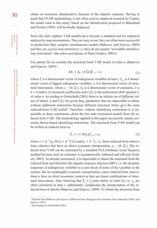
For starters let us consider the structural form VAR model of order p (Bahovec and Erjavec, 2009)3:
(1)
where Zt is k dimensional vector of endogenous variables at time t, Zt-1 is k dimen-
sional vector of lagged endogenous variables, et is k dimensional vector of struc-
tural innovations, where et ~ (0, Σ
e), A
0 is k dimensional vector of constants, A is
k × k matrix of structural coeffi cients and C(L) is the polynomial shift operator L of order p. According to Gottschalk (2001) there is an infi nite set of different val-ues of matrix A and C(L) for given data, parameters that are impossible to obtain without additional restrictions because different structural forms give the same reduced-form VAR model4. Therefore, without identifying restrictions it is im-possible to draw conclusions about the true state (structural model) from the re-duced form VAR. The methodology applied in this paper necessarily entails eco-nomic theory-based identifying restrictions. The structural form VAR model can be written in reduced form as:
(2)
where , and , i.e. those reduced-form innova-tions (shocks) that have no direct economic interpretation, u
t ~ (0, Σ
u). The re-
duced form VAR can be estimated by a standard OLS (Ordinary Least Squares) method because such an estimator is asymptotically unbiased and effi cient (End-ers, 2003). As already mentioned, it is impossible to obtain the structural from the reduced form and therefore the impulse response function (IRF), i.e. the dynamic responses of endogenous variables to a unit shock of some of the variables in the system, has no meaningful economic interpretation, since reduced-form innova-tions u
t have no direct economic context as they are linear combinations of struc-
tural innovations. Also, knowing that Σu ≠ I
K (unit matrix of order k), i.e. u
kt are
often correlated in time t, additionally complicates the interpretation of the re-duced form of shocks (Bahovec and Erjavec, 2009). To obtain the structural from
3 Notation from Bahovec and Erjavec (2009) has been changed to be consistent with Lütkepohl (2005), and McCoy (1997).4 See example in Gottschalk (2001).
RA
FAEL R
AVN
IK AN
D IVAN ŽILIĆ:
THE U
SE OF SVA
R AN
ALY
SIS IN DETER
MIN
ING TH
E EFFECTS O
F FISCA
L SHO
CK
S IN CR
OATIA
FINA
NC
IAL TH
EORY A
ND
PRA
CTIC
E35 (1) 25-58 (2011)
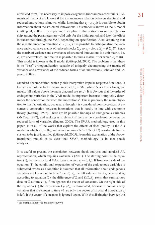
31a reduced form, it is necessary to impose exogenous (nonsample) constraints. Ele-ments of matrix A are known if the instantaneous relation between structural and reduced innovations is known, while, knowing that e
t = Au
t, it is possible to obtain
information about the structural innovations. This model is known as the A model (Lütkepohl, 2005). It is important to emphasize that restrictions on the relation-ship among the parameters are valid only for the initial period, and later the effect is transmitted through the VAR depending on specifi cation. Also, assuming that the u
t is the linear combination e
t ~ (0, I
K) it is possible to orthogonalize the vari-
ance and covariance matrix of reduced shocks Σu, so u
t = Be
t, a Σ
u = B Σ
e B´. Since
the matrix of variance and covariance of structural innovations is a unit matrix, i.e. e
kt are uncorrelated, in time t it is possible to fi nd a matrix B for which Σ
u = BB´.
This model is known as the B model (Lütkepohl, 2005). The problem is that there is no “best” orthogonalization capable of uniquely decomposing the matrix of variance and covariance of the reduced forms of an innovation (Bahovec and Er-javec, 2009).
Standard decomposition, which yields interpretive impulse response functions, is known as Choleski factorization, in which Σ
u = GG´, where G is a lower triangular
matrix (all values above the main diagonal are zero). It is obvious that the order of endogenous variables in the VAR model is important because it implicitly deter-mines the connection between the innovations5. This is precisely the main objec-tion to this factorization, because, although it is considered non-theoretical, it as-sumes a connection between innovations that is hardly in line with economic theory (Keating, 1992). There are k! possible line-ups of endogenous variables (McCoy, 1997), and ranking is irrelevant if there is no correlation between the reduced form of variables (Enders, 2003). The SVAR methodology used in this paper, as in all of the works that explore the effects of fi scal policy, is the AB model in which Au
t = Be
t, and which requires 2k2 – 1/2k (k+1) constraints for the
system to be just-identifi ed (Lütkepohl, 2005). From this explanation of the above-mentioned models it is clear that SVAR methodology is in fact shock analysis.
It is useful to present the correlation between shock analysis and standard AR representation, which explains Gottschalk (2001). The starting point is the equa-tion (1), i.e. the structural VAR form in which e
t ~ (0, I
K). If from each side of the
equation (1) the conditional expectation of vector of the endogenous variables is subtracted, where as a condition is assumed that all information about endogenous variables are known up to time t, i.e. E
t-1Z
t, the left side will be Au
t because it is,
according to equation (2), the difference of Zt and D(L)Z
t-1 (term that summarizes
data on Zt at time t-1), if one ignores the vector of constants. On the right side of
the equation (1) the expression C(L)Zt-1
is eliminated, because it contains only variables that are known to time t-1, so only the vector of structural innovation e
t
is left, if the vector of constants is ignored again. With this distinction between the
5 See example in Bahovec and Erjavec (2009).

RA
FAEL R
AVN
IK AN
D IVAN ŽILIĆ:
THE U
SE OF SVA
R AN
ALY
SIS IN DETER
MIN
ING TH
E EFFECTS O
F FISCA
L SHO
CK
S IN CR
OATIA
FINA
NC
IAL TH
EORY A
ND
PRA
CTIC
E35 (1) 25-58 (2011)
32 expected and unexpected changes in the endogenous variables, we get the A SVAR from the structural form VAR model, but equally we could get the B and AB model.
3.2 SPECIFICATION OF BLANCHARD-PEROTTI IDENTIFICATION METHODOLOGY
This section will briefl y explain SVAR methodology and the identifi cation method needed for obtaining economic interpretative impulse response functions. Thus, the reduced form VAR model of equation (2) is estimated where Z
t = [g, γ, π, p, r]´
is the vector of endogenous variables, which includes logarithms of seasonally adjusted budgetary central government expenditures g, logarithms of the seaso-nally adjusted base index of industrial production (base = 2005) y as a proxy of output, the fi rst difference of logarithms of the consumer price index π, logarithms of seasonally adjusted budgetary central government revenues p and the overnight interest rate on the money market r. The Akaike information criterion and the LM test suggest that the optimal lag order p is 5 shifts. After the reduced form of VAR is estimated with the OLS estimation method, as already mentioned, it is neces-sary to assume the exogenous coeffi cients in order to obtain structural innovations (those that have an economic interpretation) from the reduced innovations. Blan-chard and Perotti (1999) developed the methodology of structural identifi cation based on the institutional features of the tax system. The main idea is that if you take high frequency data (the mentioned authors use quarterly data), the systema-tic discretionary fi scal policy response will be slow due to data collection, and the slow implementation of discretionary measures. As in our model we use monthly data, the above argument is further accentuated. Although the structural VARs are predominantly used in the analysis of monetary policy, the discrete character of the collection and publication of fi scal variables, as opposed to the continuous character of the publication of the monetary variables, makes the analysis of fi scal policies even more suitable for this method of identifi cation. According to Perotti (2002), reduced innovations of government spending ( ) and tax revenues ( ) are considered to be a linear combination of three components: (1) the automatic responses of government spending and tax revenues to output ( ), infl ation ( ) and interest rates ( ) innovations; (2) the systematic discretionary response of economic policy on output, infl ation and interest rates innovations; (3) random discretionary shocks, i.e. structural forms of innovations of government spending ( ) and tax revenues ( ). Thus, the reduced forms of innovation of government spending and tax revenues can be formally written as:
(3)
(4)
The initial assumption that the government cannot react to shocks of other varia-bles in the same quarter or month is essential, because coeffi cients refl ect only the automatic response of government spending and tax revenue on output change,
+
+
RA
FAEL R
AVN
IK AN
D IVAN ŽILIĆ:
THE U
SE OF SVA
R AN
ALY
SIS IN DETER
MIN
ING TH
E EFFECTS O
F FISCA
L SHO
CK
S IN CR
OATIA
FINA
NC
IAL TH
EORY A
ND
PRA
CTIC
E35 (1) 25-58 (2011)
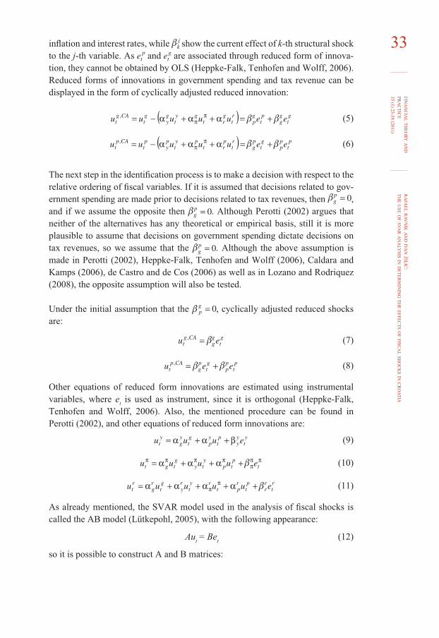
33infl ation and interest rates, while show the current effect of k-th structural shock to the j-th variable. As and are associated through reduced form of innova-tion, they cannot be obtained by OLS (Heppke-Falk, Tenhofen and Wolff, 2006). Reduced forms of innovations in government spending and tax revenue can be displayed in the form of cyclically adjusted reduced innovation:
(5)
(6)
The next step in the identifi cation process is to make a decision with respect to the relative ordering of fi scal variables. If it is assumed that decisions related to gov-ernment spending are made prior to decisions related to tax revenues, then , and if we assume the opposite then . Although Perotti (2002) argues that neither of the alternatives has any theoretical or empirical basis, still it is more plausible to assume that decisions on government spending dictate decisions on tax revenues, so we assume that the . Although the above assumption is made in Perotti (2002), Heppke-Falk, Tenhofen and Wolff (2006), Caldara and Kamps (2006), de Castro and de Cos (2006) as well as in Lozano and Rodriquez (2008), the opposite assumption will also be tested.
Under the initial assumption that the , cyclically adjusted reduced shocks are:
(7)
(8)
Other equations of reduced form innovations are estimated using instrumental variables, where e
t is used as instrument, since it is orthogonal (Heppke-Falk,
Tenhofen and Wolff, 2006). Also, the mentioned procedure can be found inPerotti (2002), and other equations of reduced form innovations are:
(9)
(10)
(11)
As already mentioned, the SVAR model used in the analysis of fi scal shocks is called the AB model (Lütkepohl, 2005), with the following appearance:
Aut = Be
t (12)
so it is possible to construct A and B matrices:

RA
FAEL R
AVN
IK AN
D IVAN ŽILIĆ:
THE U
SE OF SVA
R AN
ALY
SIS IN DETER
MIN
ING TH
E EFFECTS O
F FISCA
L SHO
CK
S IN CR
OATIA
FINA
NC
IAL TH
EORY A
ND
PRA
CTIC
E35 (1) 25-58 (2011)
34
(13)
To make the system just-identifi ed, 2k2 – 1/2k (k + 1), i.e. 35 constraints (k is the number of endogenous variables) should be imposed in total in both matrices. Matrix B has 19 coeffi cients that are equal to zero, and the main diagonal of ma-trix A provides another 5 restrictions. All coeffi cients associated with the equation of reduced innovation in government spending are set to zero, except for the im-pact of infl ation on government spending, which is assumed to be -0.5, because the expenditures for wages of public employees, who constitute a signifi cant share of government spending, are not indexed to infl ation in the same period. This re-lationship of infl ation and government spending is taken from Caldara and Kamps (2006), Lozano and Rodriquez (2008), and Štikova (2006). All other coeffi cients associated with reduced innovation in government spending are zero, because government spending is entirely under the control of economic policy, which can not react in the same period and the effect is not automatic because it is a variable whose dynamics is solely infl uenced by government decisions. These arguments give 4 additional restrictions. Furthermore, the assumption that overnight interest rates-reduced innovation does not affect any one of the remaining four reduced innovations provides 3 more restrictions. As the impact of government expendi-ture on tax revenues can be modelled in a matrix B with structural innovations, the relationship in matrix A is assumed to be zero. Also, it is assumed that the reduced form innovation of infl ation is not affected during the same period by the reduced form of output, which gives 2 more restrictions. The remaining two restrictions necessary for the system to be just-identifi ed are obtained by calculating the im-pact of reduced innovation of output on reduced innovations of tax (exogenous elasticity 0.95) and the impact of reduced innovation of infl ation on reduced in-novation of taxes (exogenous elasticity 0.89), using a methodology that will be explained below. Such a methodology for exact SVAR identifi cation was also used in Lozano and Rodriquez (2008), Štikova (2006), and Caldara and Kamps (2008).
It is necessary to point out some facts regarding the nature of the fi scal shocks whose effects we are observing. Shocks and represent a one-time increase in revenues or expenditures by one standard deviation compared to the average of the period. Perotti (2002) points out that although one can argue that due to the nature of the budget process there is only one fi scal shock per year, in practice the fi scal authorities with numerous revisions and changes in tax policy often change the course of fi scal policy. Bernanke and Mihov (1996), while discussing mone-tary shocks, stress the importance of some technical facts. Since the fi scal shock
RA
FAEL R
AVN
IK AN
D IVAN ŽILIĆ:
THE U
SE OF SVA
R AN
ALY
SIS IN DETER
MIN
ING TH
E EFFECTS O
F FISCA
L SHO
CK
S IN CR
OATIA
FINA
NC
IAL TH
EORY A
ND
PRA
CTIC
E35 (1) 25-58 (2011)
35cannot be viewed in the context of the variables in the model (except for the fi scal variables, output, infl ation and short-term interest rate), the shock of fi scal varia-bles cannot be interpreted through the initial movement of these variables. The authors mentioned explain the causes of shocks6: (1) the fi scal authorities have imperfect information about the current state of the economy, (2) changes in the relative weights that fi scal authorities place on various budget spending. The fi rst cause is explicitly assumed in the model identifi cation, while the second one is explained by the fact that the process of making decisions about government spending is largely infl uenced by the struggle of various interest or social groups for greater government spending, so the weights the state puts on various forms of spending are constantly changing.
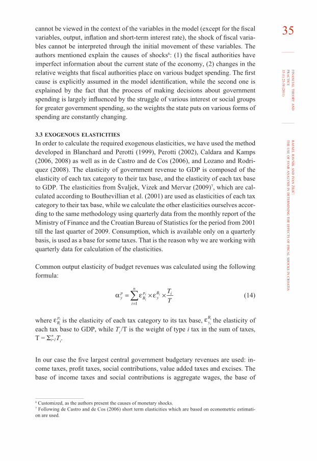
3.3 EXOGENOUS ELASTICITIES
In order to calculate the required exogenous elasticities, we have used the method developed in Blanchard and Perotti (1999), Perotti (2002), Caldara and Kamps (2006, 2008) as well as in de Castro and de Cos (2006), and Lozano and Rodri-quez (2008). The elasticity of government revenue to GDP is composed of the elasticity of each tax category to their tax base, and the elasticity of each tax base to GDP. The elasticities from Švaljek, Vizek and Mervar (2009)7, which are cal-culated according to Bouthevillian et al. (2001) are used as elasticities of each tax category to their tax base, while we calculate the other elasticities ourselves accor-ding to the same methodology using quarterly data from the monthly report of the Ministry of Finance and the Croatian Bureau of Statistics for the period from 2001 till the last quarter of 2009. Consumption, which is available only on a quarterly basis, is used as a base for some taxes. That is the reason why we are working with quarterly data for calculation of the elasticities.
Common output elasticity of budget revenues was calculated using the following formula:
(14)
where is the elasticity of each tax category to its tax base, the elasticity of each tax base to GDP, while T
i /T is the weight of type i tax in the sum of taxes,
T = Σi=1 Ti.
In our case the fi ve largest central government budgetary revenues are used: in-come taxes, profi t taxes, social contributions, value added taxes and excises. The base of income taxes and social contributions is aggregate wages, the base of
6 Customized, as the authors present the causes of monetary shocks.7 Following de Castro and de Cos (2006) short term elasticities which are based on econometric estimati-on are used.
n

RA
FAEL R
AVN
IK AN
D IVAN ŽILIĆ:
THE U
SE OF SVA
R AN
ALY
SIS IN DETER
MIN
ING TH
E EFFECTS O
F FISCA
L SHO
CK
S IN CR
OATIA
FINA
NC
IAL TH
EORY A
ND
PRA
CTIC
E35 (1) 25-58 (2011)
36 profi t tax is gross operating surplus,8 while the base of indirect taxes is private consumption. As noted above, T = Σi=1 Ti
is the sum of fi ve revenues, so Ti /T is a
simple weight of each revenue, which we multiply with the output elasticity to each base and the base elasticity to the corresponding revenue, in order to obtain a single elasticity . These shares were obtained from the average share of indi-vidual taxes as well as in Heppke-Falk, Tenhofen and Wolf (2006), while the values and are calculated according to the methodology described in Loz-ano and Rodriques (2008). In table 1 the calculations of all elasticities are shown, where the output elasticity of taxes equals 0.95. Comparing our results with the results of other papers, we see that our elasticity almost matches the elasticity obtained in the work Heppke-Falk, Tenhofen and Wolf (2006) for the case of Germany (also about 0.95), while that in Perotti (2002) is 0.92. For Spain, an elasticity of 0.62 is calculated (de Castro and de Cos, 2006), for the USA 1.85, UK 0.76, Australia 0.81 and 1.86 for Canada (Perotti, 2002). We conclude that the results for Croatia do not signifi cantly differ from those in other countries.
TABLE 1The elasticity of government revenue in relation to output
Revenue Ti /T
Income tax 2.32 0.88 2.05 0.07
Profi t tax 2.12 1.03 2.20 0.12
Value added tax 1.13 0.79 0.89 0.35
Excises 0.50 0.79 0.40 0.11
Social contributions 0.62 0.80 0.50 0.35
0.95
Note: Values rounded upwards to two decimal places.Source: Authors’ calculations, and Švaljek, Vizek and Mervar (2009).
We have calculated not only the output elasticity but also the infl ation elasticity, according to the above methodology, with certain modifi cations. Although there are signifi cant differences among the methodologies used to calculate the elasti-city of budget revenue to infl ation, we are using the algorithm developed in Per-otti (2002), and de Castro and de Cos (2006). Due to the proportionality of the price level with indirect taxes, these authors assumed that the elasticity of profi t taxes in relation to infl ation, as well as the elasticity of indirect taxes in relation to infl ation amounts to 0. Other values are calculated as in the case of output. This
8 Gross operating surpluss is calculated according the same methodology as in Švaljek, Vizek and Mervar (2009) (the total wages are subtracted from the GDP).
n
RA
FAEL R
AVN
IK AN
D IVAN ŽILIĆ:
THE U
SE OF SVA
R AN
ALY
SIS IN DETER
MIN
ING TH
E EFFECTS O
F FISCA
L SHO
CK
S IN CR
OATIA
FINA
NC
IAL TH
EORY A
ND
PRA
CTIC
E35 (1) 25-58 (2011)
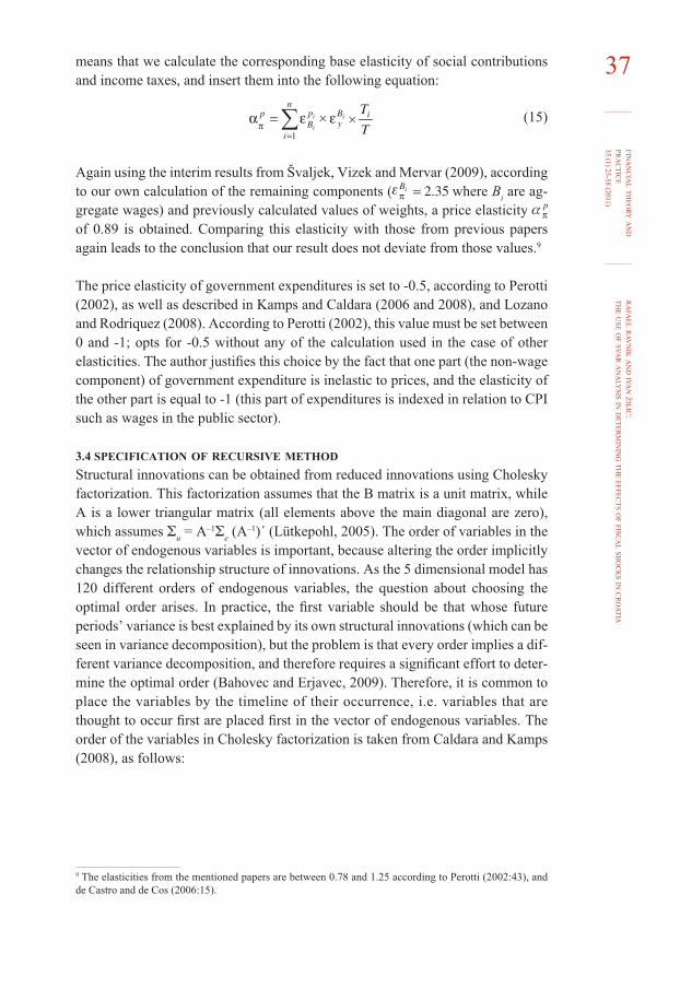
37means that we calculate the corresponding base elasticity of social contributions and income taxes, and insert them into the following equation:
(15)
Again using the interim results from Švaljek, Vizek and Mervar (2009), according to our own calculation of the remaining components ( where B
i are ag-
gregate wages) and previously calculated values of weights, a price elasticity of 0.89 is obtained. Comparing this elasticity with those from previous papers again leads to the conclusion that our result does not deviate from those values.9
The price elasticity of government expenditures is set to -0.5, according to Perotti (2002), as well as described in Kamps and Caldara (2006 and 2008), and Lozano and Rodriquez (2008). According to Perotti (2002), this value must be set between 0 and -1; opts for -0.5 without any of the calculation used in the case of other elasticities. The author justifi es this choice by the fact that one part (the non-wage component) of government expenditure is inelastic to prices, and the elasticity of the other part is equal to -1 (this part of expenditures is indexed in relation to CPI such as wages in the public sector).
3.4 SPECIFICATION OF RECURSIVE METHOD
Structural innovations can be obtained from reduced innovations using Cholesky factorization. This factorization assumes that the B matrix is a unit matrix, while A is a lower triangular matrix (all elements above the main diagonal are zero), which assumes Σ
u = A–1Σ
e (A–1)´ (Lütkepohl, 2005). The order of variables in the
vector of endogenous variables is important, because altering the order implicitly changes the relationship structure of innovations. As the 5 dimensional model has 120 different orders of endogenous variables, the question about choosing the optimal order arises. In practice, the fi rst variable should be that whose future periods’ variance is best explained by its own structural innovations (which can be seen in variance decomposition), but the problem is that every order implies a dif-ferent variance decomposition, and therefore requires a signifi cant effort to deter-mine the optimal order (Bahovec and Erjavec, 2009). Therefore, it is common to place the variables by the timeline of their occurrence, i.e. variables that are thought to occur fi rst are placed fi rst in the vector of endogenous variables. The order of the variables in Cholesky factorization is taken from Caldara and Kamps (2008), as follows:
9 The elasticities from the mentioned papers are between 0.78 and 1.25 according to Perotti (2002:43), and de Castro and de Cos (2006:15).
RA
FAEL R
AVN
IK AN
D IVAN ŽILIĆ:
THE U
SE OF SVA
R AN
ALY
SIS IN DETER
MIN
ING TH
E EFFECTS O
F FISCA
L SHO
CK
S IN CR
OATIA
FINA
NC
IAL TH
EORY A
ND
PRA
CTIC
E35 (1) 25-58 (2011)
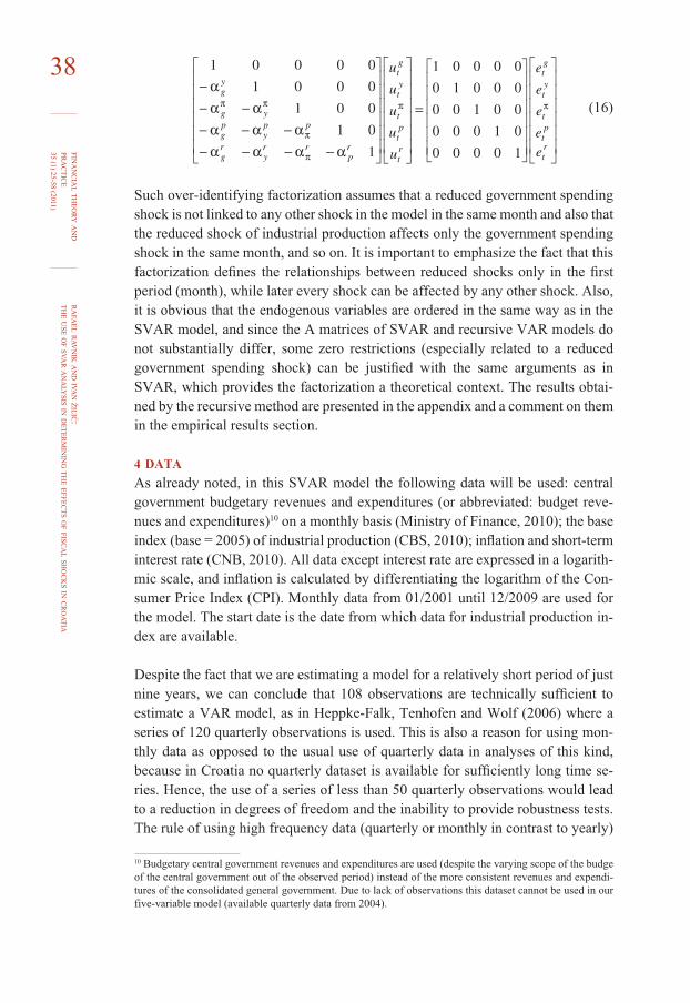
38
(16)
Such over-identifying factorization assumes that a reduced government spending shock is not linked to any other shock in the model in the same month and also that the reduced shock of industrial production affects only the government spending shock in the same month, and so on. It is important to emphasize the fact that this factorization defi nes the relationships between reduced shocks only in the fi rst period (month), while later every shock can be affected by any other shock. Also, it is obvious that the endogenous variables are ordered in the same way as in the SVAR model, and since the A matrices of SVAR and recursive VAR models do not substantially differ, some zero restrictions (especially related to a reduced government spending shock) can be justifi ed with the same arguments as in SVAR, which provides the factorization a theoretical context. The results obtai-ned by the recursive method are presented in the appendix and a comment on them in the empirical results section.
4 DATA As already noted, in this SVAR model the following data will be used: central government budgetary revenues and expenditures (or abbreviated: budget reve-nues and expenditures)10 on a monthly basis (Ministry of Finance, 2010); the base index (base = 2005) of industrial production (CBS, 2010); infl ation and short-term interest rate (CNB, 2010). All data except interest rate are expressed in a logarith-mic scale, and infl ation is calculated by differentiating the logarithm of the Con-sumer Price Index (CPI). Monthly data from 01/2001 until 12/2009 are used for the model. The start date is the date from which data for industrial production in-dex are available.
Despite the fact that we are estimating a model for a relatively short period of just nine years, we can conclude that 108 observations are technically suffi cient to estimate a VAR model, as in Heppke-Falk, Tenhofen and Wolf (2006) where a series of 120 quarterly observations is used. This is also a reason for using mon-thly data as opposed to the usual use of quarterly data in analyses of this kind, because in Croatia no quarterly dataset is available for suffi ciently long time se-ries. Hence, the use of a series of less than 50 quarterly observations would lead to a reduction in degrees of freedom and the inability to provide robustness tests. The rule of using high frequency data (quarterly or monthly in contrast to yearly)
10 Budgetary central government revenues and expenditures are used (despite the varying scope of the budge of the central government out of the observed period) instead of the more consistent revenues and expendi-tures of the consolidated general government. Due to lack of observations this dataset cannot be used in our five-variable model (available quarterly data from 2004).

RA
FAEL R
AVN
IK AN
D IVAN ŽILIĆ:
THE U
SE OF SVA
R AN
ALY
SIS IN DETER
MIN
ING TH
E EFFECTS O
F FISCA
L SHO
CK
S IN CR
OATIA
FINA
NC
IAL TH
EORY A
ND
PRA
CTIC
E35 (1) 25-58 (2011)
39to eliminate the impact of discretionary fi scal policy (Blanchard and Perotti, 1999; and Perotti, 2002) also confi rms our decision to use monthly data. However, in reaching conclusions it should be taken into account that results in the form of impulse response functions for output actually show industrial production, the dynamics of which are not equivalent to the dynamics of GDP. Another shortco-ming is the impossibility of simulating fi scal shocks to GDP components, i.e. showing responses of investment and private consumption to fi scal shocks because these data are published in quarterly frequency.
The appendix presents the original and seasonally adjusted series of budget revenue and expenditures on a monthly basis expressed in a logarithmic scale (LNPRI and LNRAS stands for original and LNPRI_SA LNRAS_SA for seasonally adjusted values). Seasonal adjustment is performed using the U.S. Census Bureau X12-ARI-MA method with the program package Eviews 5.0. It is important to emphasize that these are nominal variables, as is usual in describing the impact of fi scal shocks on real variables. Viewing the appendix it is possible to compare the seasonality of revenues and expenditures and conclude that budget revenues show signifi cantly stronger seasonal fl uctuations than budget expenditures do. Despite these minor seasonal fl uctuations, we also use seasonally adjusted time series for budgetary expenditures, which is consistent with the standard literature. The other variables are also shown in the appendix. It should be noted that due to very strong seasonal fl uctuations the index of industrial production is also seasonally adjusted by the same method, while seasonal adjustment is not applied to interest rate or infl ation.
Monthly consumer price base-index is taken from the Croatian National Bank (base = 2005), and infl ation is derived according the previously described manner. The short-term interest rate on interbank demand deposit trading is used as the reference interest rate, and it is measured as a weighted monthly average (also downloaded from the database of the Croatian National Bank).
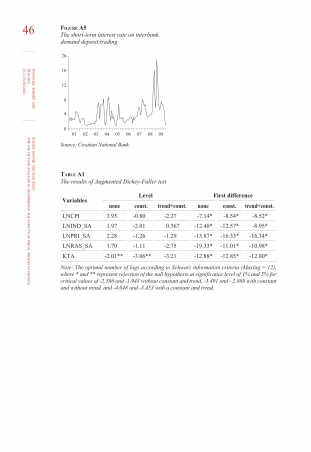
Unit root test is also performed (table A1) from which it can be concluded that at the 5% signifi cance level only the interest rate is stationary in levels, while the other variables contain unit roots in levels and are stationary only in fi rst differen-ces. At 1% signifi cance all variables contain unit roots in levels and are stationary in fi rst differences. Despite the fact that the variables contain unit roots, variables in levels will be used in this analysis, which is common practice in such studies (Perotti, 2002; de Castro and de Cos, 2006; and Heppke-Falk, Tenhofen and Wolf, 2006) because of our primary interest in the dynamics, rather than parameter esti-mation.
5 EMPIRICAL RESULTS
The impulse response functions, the matrices with the estimated parameters and the variance decomposition are given in the appendix. All results were obtained by using Eviews 5.0 software. In table A2 matrices A and B are shown, while in table A3 the variance decomposition of the baseline model can be seen.
RA
FAEL R
AVN
IK AN
D IVAN ŽILIĆ:
THE U
SE OF SVA
R AN
ALY
SIS IN DETER
MIN
ING TH
E EFFECTS O
F FISCA
L SHO
CK
S IN CR
OATIA
FINA
NC
IAL TH
EORY A
ND
PRA
CTIC
E35 (1) 25-58 (2011)
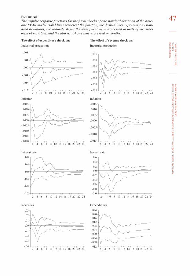
40 In fi gure A6 and fi gure A9 impulse response functions for both methods used (recursive and structural) are shown. Dashed lines represent the intervals of two standard deviations, while the solid lines represent the impulse function.
While interpreting the fi scal variable shocks one should have in mind that shocks from government expenditures or revenues are not caused by any of the other variables in the model, because the structural shocks are derived from residuals of the VAR equation.
The effect of expenditure shock on industrial production (see fi gure A6), which we use as a proxy variable of output, unlike previous research into effects of fi scal policy in Croatia (Rukelj, 2009; and Benavides, 2006), was negative in the short term. The mentioned effect vanishes within two years and throughout the entire period the effect is in the performance range of ± 0.5 units of measurement of variable. A possible explanation of this unconventional direction of infl uence may be the predominant effect of the crowding out of private investment as against the output effect. An additional problem is the unavoidable choice of industrial pro-duction as the only suffi ciently long monthly series that serves as an approxima-tion of economic activity. Despite the unexpected result, similar conclusions are found in Heppke-Falk, Tenhofen and Wolf (2006), and Lozano and Rodriguez (2008). In de Castro and de Cos (2006) positive short-term turns into a negative long-term effect.
Revenue shock on industrial production has a negative effect in the fi rst three months after which it turns into a positive, but volatile effect. After 10 months the effect stabilizes and does not vanish, which is probably connected with the fact that the tax shock has a permanent impact on the taxes because a change in tax rates has a lasting effect on the amount of tax revenue. Such a lasting positive reaction of economic activity was obtained in Falk, Tenhofen and Wolf (2006), and Lozano and Rodriguez (2008). De Castro and de Cos (2006) also present a short-term positive effect, which in the long run turns into a negative effect; while in Štikova (2006) government revenue shocks have no impact on GDP.
Both fi scal shocks have a minimal effect on infl ation (within 0.007 units of mea-surement of variable) that vanishes within a year. The initial two-month expendi-ture shock effect on infl ation is positive when it turns to the negative effect which prevails until the eighth month, which is consistent with the textbook knowledge of the economic policy of stable exchange rate (see Gartner, 2006; Mankiw, 2007; etc.). A tax shock raises infl ation the fi rst six months and then it stabilizes in spite of the presence of the permanent effect of taxes. This is because the shock is im-plemented in the infl ationary expectations after one year. In other studies based on SVAR methodology the short-term effect of fi scal shocks on infl ation is volatile and in the long term also negligible.
RA
FAEL R
AVN
IK AN
D IVAN ŽILIĆ:
THE U
SE OF SVA
R AN
ALY
SIS IN DETER
MIN
ING TH
E EFFECTS O
F FISCA
L SHO
CK
S IN CR
OATIA
FINA
NC
IAL TH
EORY A
ND
PRA
CTIC
E35 (1) 25-58 (2011)
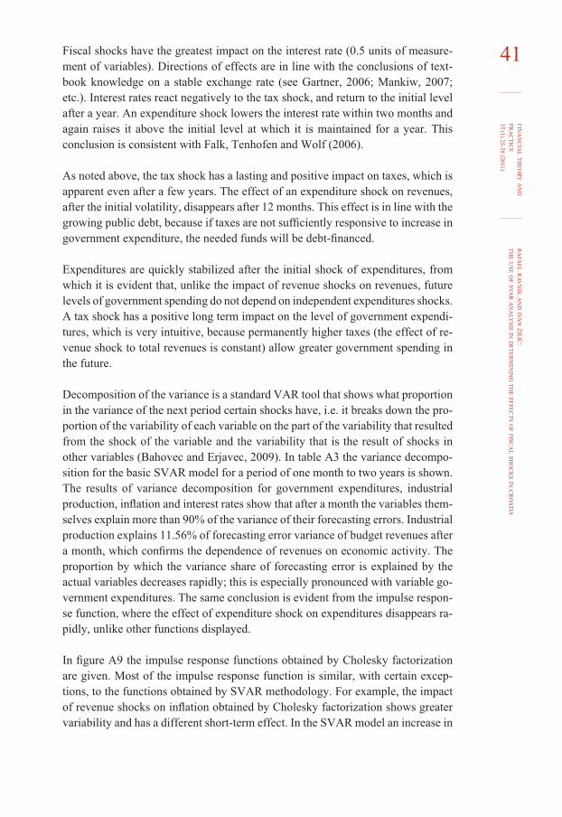
41Fiscal shocks have the greatest impact on the interest rate (0.5 units of measure-ment of variables). Directions of effects are in line with the conclusions of text-book knowledge on a stable exchange rate (see Gartner, 2006; Mankiw, 2007; etc.). Interest rates react negatively to the tax shock, and return to the initial level after a year. An expenditure shock lowers the interest rate within two months and again raises it above the initial level at which it is maintained for a year. This conclusion is consistent with Falk, Tenhofen and Wolf (2006).
As noted above, the tax shock has a lasting and positive impact on taxes, which is apparent even after a few years. The effect of an expenditure shock on revenues, after the initial volatility, disappears after 12 months. This effect is in line with the growing public debt, because if taxes are not suffi ciently responsive to increase in government expenditure, the needed funds will be debt-fi nanced.
Expenditures are quickly stabilized after the initial shock of expenditures, from which it is evident that, unlike the impact of revenue shocks on revenues, future levels of government spending do not depend on independent expenditures shocks. A tax shock has a positive long term impact on the level of government expendi-tures, which is very intuitive, because permanently higher taxes (the effect of re-venue shock to total revenues is constant) allow greater government spending in the future.
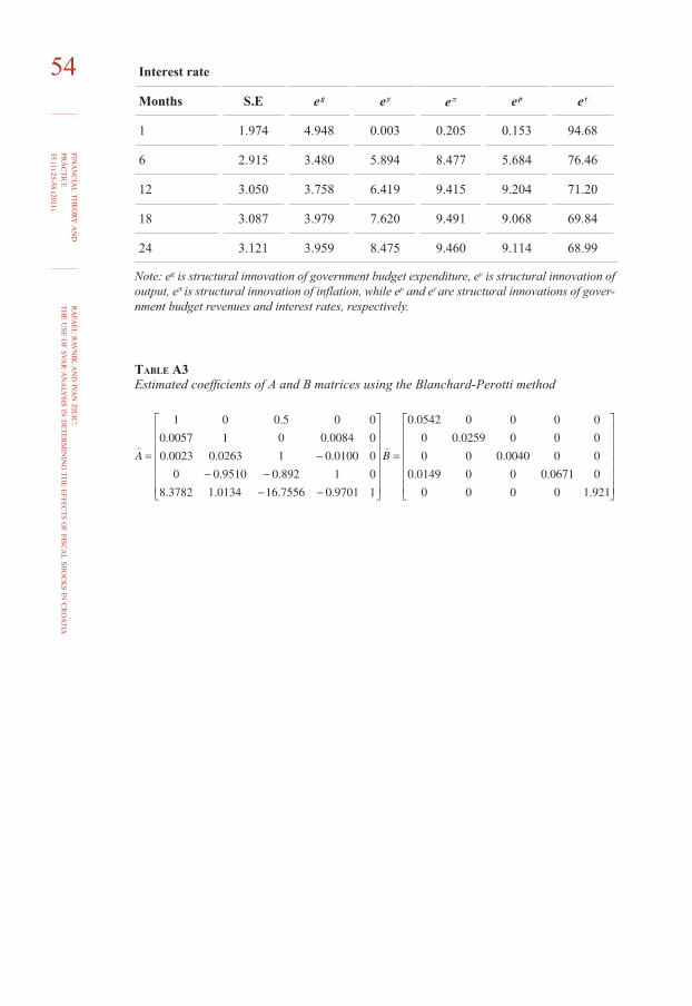
Decomposition of the variance is a standard VAR tool that shows what proportion in the variance of the next period certain shocks have, i.e. it breaks down the pro-portion of the variability of each variable on the part of the variability that resulted from the shock of the variable and the variability that is the result of shocks in other variables (Bahovec and Erjavec, 2009). In table A3 the variance decompo-sition for the basic SVAR model for a period of one month to two years is shown. The results of variance decomposition for government expenditures, industrial production, infl ation and interest rates show that after a month the variables them-selves explain more than 90% of the variance of their forecasting errors. Industrial production explains 11.56% of forecasting error variance of budget revenues after a month, which confi rms the dependence of revenues on economic activity. The proportion by which the variance share of forecasting error is explained by the actual variables decreases rapidly; this is especially pronounced with variable go-vernment expenditures. The same conclusion is evident from the impulse respon-se function, where the effect of expenditure shock on expenditures disappears ra-pidly, unlike other functions displayed.
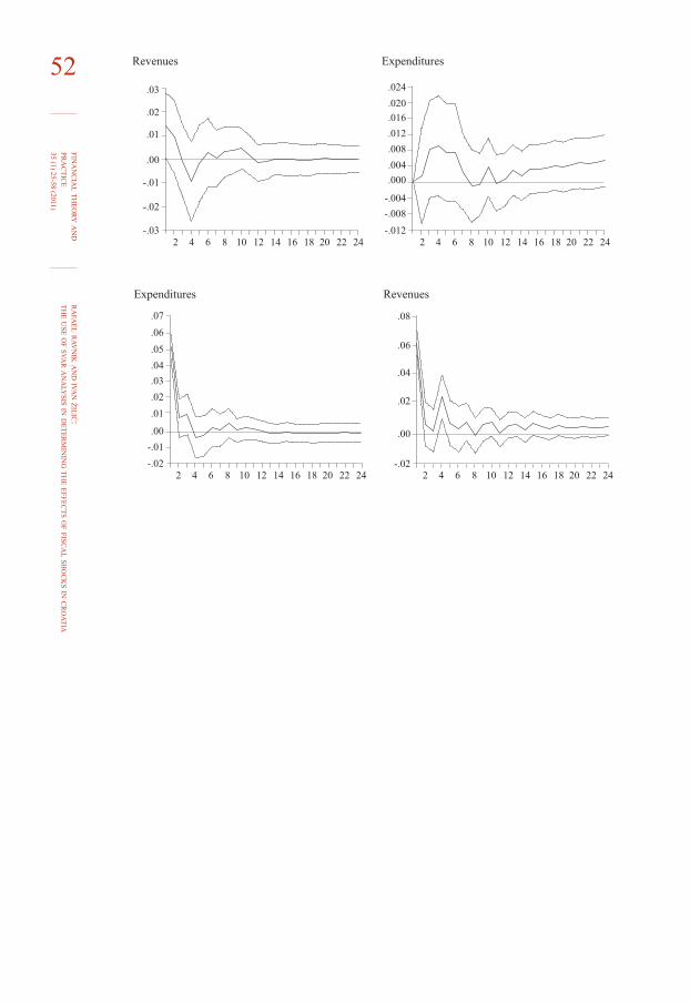
In fi gure A9 the impulse response functions obtained by Cholesky factorization are given. Most of the impulse response function is similar, with certain excep-tions, to the functions obtained by SVAR methodology. For example, the impact of revenue shocks on infl ation obtained by Cholesky factorization shows greater variability and has a different short-term effect. In the SVAR model an increase in
RA
FAEL R
AVN
IK AN
D IVAN ŽILIĆ:
THE U
SE OF SVA
R AN
ALY
SIS IN DETER
MIN
ING TH
E EFFECTS O
F FISCA
L SHO
CK
S IN CR
OATIA
FINA
NC
IAL TH
EORY A
ND
PRA
CTIC
E35 (1) 25-58 (2011)
42 infl ation is instantaneous, while in the recursive model infl ation rises after a few months. Also, the difference in short-term effects between SVAR methodology and recursive approach is apparent while observing the effects of expenditure shocks on revenues and revenue shock on expenditures.
6 ROBUSTNESS CHECK
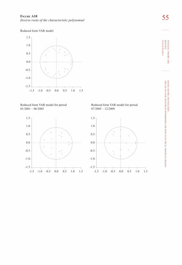
The fi rst stability condition, which indicates that all roots of the characteristic polynomial are inside the unit circle, is satisfi ed, so the defi ned VAR model is stable.11
An additional stability and robustness check is the comparison of the SVAR mod-el with the VAR model, which uses the Cholesky decomposition. The order of variables was previously mentioned, and the number of lags is again fi ve accord-ing to the Akaike information criterion and LM test. The impulse response func-tions for the recursive approach can be seen in fi gure A9 and have been described above.
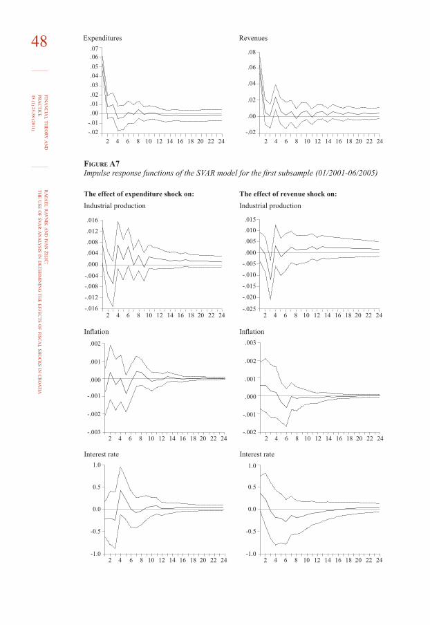
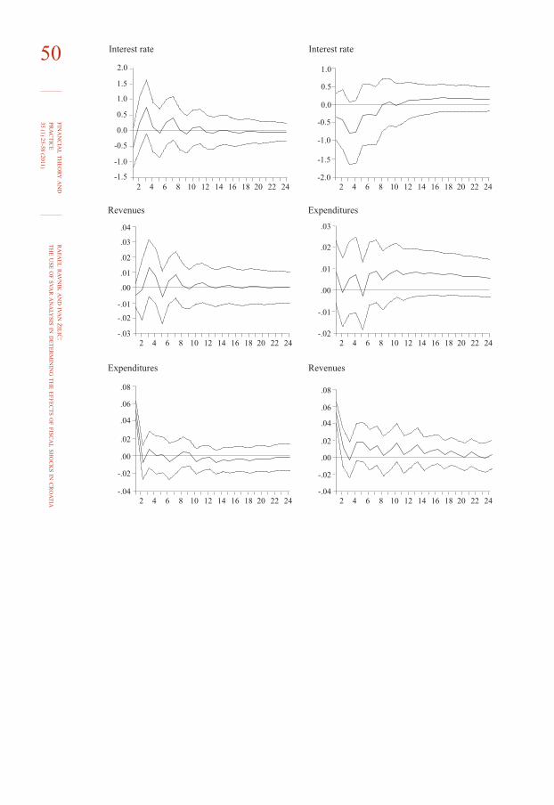
The most common method for checking the robustness of SVAR models is the breakpoint test, where the series is divided into two parts. In this case, the series is divided into two equal samples where the fi rst subsample covers the period from 01/2001 to 06/2005 and the second subsample from 07/2005 to 12/2009. Impulse response functions for two models according to these two series are given in fi gures A7 and A8. The same method of identifi cation as for the whole series is used, and the number of lags is also chosen according to the lag length criterion tests. Both indicators (Akaike info criterion and LM test) suggest three lags for the second model. For the fi rst model the Akaike information criterion suggests fi ve, while the LM test suggests three lags. Since it is a relatively short series, but also because of the lag selection in the second series, we have decided also to use three lags in the model for the fi rst sample. In addition, the lag exclusion test shows that the fourth shift is not signifi cant, which further confi rms our selection decision.
The purpose of dividing the series into two parts is to investigate the similarity between the responses of variables to shocks in each sample. The impulse re-sponse function differs most signifi cantly for the case of the reaction of industrial production to an expenditure shock. In contrast to the model for the fi rst sample where the effect is slightly positive, in the second sample this effect is negative, as well as for the total sample. These results may occur due to several factors. There is a possibility of an impact of structural changes in the observed period, which may lead to differences in the results. One reason may be the wrong selection of variables, i.e. in the case of industrial production; however, also the wrong speci-fi cation of model could be the reason. The latter is possible, but the fact that for all other variables a clearly consistent response to fi scal shocks in both models is vis-ible leads us to the opposite conclusion.
11 The graph is given in figure A10.

RA
FAEL R
AVN
IK AN
D IVAN ŽILIĆ:
THE U
SE OF SVA
R AN
ALY
SIS IN DETER
MIN
ING TH
E EFFECTS O
F FISCA
L SHO
CK
S IN CR
OATIA
FINA
NC
IAL TH
EORY A
ND
PRA
CTIC
E35 (1) 25-58 (2011)
43In addition to this breakpoint test, several tests to examine the robustness of our model and the credibility of the results are conducted. Such tests are related to the selection of coeffi cient values which are not obtained by computation. The fi rst test is the examination of the sensitivity of the model results to the change of the parameter α
πg (price elasticity of budget expenditures). Earlier it was explained
why the value -0.5 is chosen according to Perotti (2002), but it is also said that this value should be somewhere between -1 and 0. Both extreme cases are examined and the results remain unchanged. The remaining parameter that is not obtained by computation, or is selected because of special assumptions is the parameter β
pg.
It was assumed that this parameter has to equal 0, which means that one believes that expenditure decisions are prior to tax decisions. An alternative to this case is that β
pg is estimated in the usual manner (by OLS), and that β
pg is set to zero, which
means that one believes that expenditure decisions will follow tax decisions. As in the previous case, the change of this parameter do not change the result signifi -cantly, which further confi rms our model specifi cation and the robustness of our SVAR model.
7 CONCLUSIONS
In this paper we have used the Blanchard-Perotti method for the identifi cation of a structural vector autoregressive model in a disaggregated analysis of the macroeconomic effects of fi scal policy shocks for the case of Croatia. Unlike the usual quarterly frequency, monthly data are used in our analysis which also provi-des the theoretical assumptions required for model to be just-identifi ed. For this reason in addition to zero restrictions, estimated exogenous elasticities of budget revenues to economic activity and infl ation are included in our model. These pro-cedures were necessary to get structural innovations from the reduced form VAR model residuals, and also to get the associated economic interpretive impulse re-sponse functions. The robustness of the model and the model specifi cation is con-fi rmed by dividing the sample into two parts as well as by other robustness checks. The sensitivity of the model to the change of the arbitrarily chosen coeffi cient of infl ation innovation impact on government spending was also tested, which is an additional confi rmation of the accurate model specifi cation.
According to the impulse response functions we can conclude that: (1) the interest rate shows the relatively strongest response to fi scal shocks, while infl ation shows the weakest response, (2) the effect of budget revenue shock on budget revenue is permanent, while the effect of budget expenditures on budget expenditure shock is instantaneous, from which we can draw intuitive conclusions about the cross-impacts of expenditures to revenues, and vice versa, (3) the effect of spending shocks on revenues is instantaneous, which confi rms the hypothesis about the tendency of the growth in public debt, (4) the impact of fi scal shocks on infl ation and interest rates is mostly economic intuitive. Revenue shock in the short term increases the rate of infl ation and also reduces the short-term interest rate, while after one year stabilization occurs at the initial level. An expenditure shock de-
RA
FAEL R
AVN
IK AN
D IVAN ŽILIĆ:
THE U
SE OF SVA
R AN
ALY
SIS IN DETER
MIN
ING TH
E EFFECTS O
F FISCA
L SHO
CK
S IN CR
OATIA
FINA
NC
IAL TH
EORY A
ND
PRA
CTIC
E35 (1) 25-58 (2011)
44 creases infl ation in the short run, while in the medium run, infl ation increases above the initial level, while the interest rate acts in the opposite direction. Such conclusions about infl ation and the interest rate could be explained by economic theory only if one assumes that the reaction of output is intuitive as well, but as the effects on industrial production are not as common (the tax shock leads to an in-crease in industrial production, while the expenditure shock reduces industrial production), it can be assumed that the index of industrial production is an inade-quate proxy variable of output. The assumption of a wrong proxy variable selec-tion may not be the only reason for such an unexpected result, because some pa-pers using direct GDP as the variable for economic activity also deal with similar unexpected results, (5) furthermore, government revenue and expenditure shocks, if implemented by the same volume in different directions do not yield the same results, i.e. fi scal expansions and contractions do not show a mirror effect on the impulse response functions.
We believe that the contribution of this paper is in its study of the consequences of fi scal policy on infl ation and the interest rate, and separately observing the ef-fects of fi scal policy instruments, as well as testing their mutual infl uence.
The applied methodology and conclusions of our paper can serve as a benchmark for comparison with the results of future research about the effects of fi scal policy using other methods, such as the fi scal dummy approach, Bayesian structural VAR models, or even theoretically dynamic stochastic general equilibrium mo-dels. One possibility for an extension of our model is the inclusion of additional variables in the existing SVAR model. Besides that, the question about the right selection of a proxy variable for economic activity is still not answered. One pos-sible solution is the implementation of a complex composite index of economic activity that in addition to industrial production includes a variety of other varia-bles in order better to approximate the movement of overall economic activity. Only when a long enough sample of national accounts is available, it will be pos-sible to examine the effects of fi scal shocks on GDP and the components of GDP (private consumption and aggregate investment).

RA
FAEL R
AVN
IK AN
D IVAN ŽILIĆ:
THE U
SE OF SVA
R AN
ALY
SIS IN DETER
MIN
ING TH
E EFFECTS O
F FISCA
L SHO
CK
S IN CR
OATIA
FINA
NC
IAL TH
EORY A
ND
PRA
CTIC
E35 (1) 25-58 (2011)
45APPENDIX
FIGURE A1 The original and seasonally adjusted va-lues of the budgetary central government revenues expressed in logarithms
FIGURE A3 The original and seasonally adjusted base index (base = 2005) of industrial production expressed in logarithms
FIGURE A2The original and seasonally adjusted va-lues of the budgetary central government expenditures expressed in logarithms
FIGURE A4Monthly infl ation (differenced logarithms of the CPI)
00 0014.4
4.5
14.8
-.010
14.8
4.6
15.2
-.005
15.2
4.7
15.6
.000
15.6
4.8
16.0
.005
16.0
4.9
16.4
.010
16.4
5.0
5.1
16.8
.015
01
01
0102
02
0203
03
0304
04
0405
05
0506
06
0607
07
0708
08
0809
09
09
LNPRI LNPRI_SA
LNIND_SA LNIND
LNRAS_SA LNRAS
Source: Ministry of Finance.
Source: Croatian Bureau of Statistics.
Source: Ministry of Finance.
Source: Croatian National Bank.
01 02 03 04 05 06 07 08 09
RA
FAEL R
AVN
IK AN
D IVAN ŽILIĆ:
THE U
SE OF SVA
R AN
ALY
SIS IN DETER
MIN
ING TH
E EFFECTS O
F FISCA
L SHO
CK
S IN CR
OATIA
FINA
NC
IAL TH
EORY A
ND
PRA
CTIC
E35 (1) 25-58 (2011)
46
TABLE A1The results of Augmented Dickey-Fuller test
VariablesLevel First difference
none const. trend+const. none const. trend+const.
LNCPI 3.95** -0.80** -2.27* -7.14* -8.54* -8.52*
LNIND_SA 1.97** -2.01** 0.367 -12.40* -12.57* -8.95*
LNPRI_SA 2.28** -1.26** -1.29* -15.87* -16.33* -16.34*
LNRAS_SA 1.70** -1.11** -2.75* -19.33* -11.01* -10.98*
KTA -2.01** -3.06** -3.21* -12.88* -12.85* -12.80*
Note: The optimal number of lags according to Schwarz information criteria (Maxlag = 12), where * and ** represent rejection of the null hypothesis at significance level of 1% and 5% for critical values of -2.586 and -1.943 without constant and trend, -3.491 and - 2.888 with constant and without trend, and -4.048 and -3.453 with a constant and trend.
FIGURE A5The short-term interest rate on interbank demand deposit trading
Source: Croatian National Bank.
0
4
8
12
16
20
01 02 03 04 05 06 07 08 09
RA
FAEL R
AVN
IK AN
D IVAN ŽILIĆ:
THE U
SE OF SVA
R AN
ALY
SIS IN DETER
MIN
ING TH
E EFFECTS O
F FISCA
L SHO
CK
S IN CR
OATIA
FINA
NC
IAL TH
EORY A
ND
PRA
CTIC
E35 (1) 25-58 (2011)
47FIGURE A6The impulse response functions for the fi scal shocks of one standard deviation of the base-line SVAR model (solid lines represent the function, the dashed lines represent two stan-dard deviations, the ordinate shows the level phenomena expressed in units of measure-ment of variables, and the abscissa shows time expressed in months)
2 2
2
2
2
2
2
2
-.012 -.015
-.0015
-0.8
-.0015
-0.8
-.0020
-1.2
-.04
-.03
-.02
-.01
.00
.01
.02
.03
-1.0
-.012-.008-.004.000.004.008.012.016.020.024
-.010
-.0010-.0010
-0.6
-.008-.005
-.0005
-0.4
-.0005
-0.4
-.004.000
.0000
0.0
.0000
-0.2
.000 .005
.0005
0.4
.0005
0.0
.004 .010
.0010 .0010
0.2
0.4
0.6
.008 .015
.0015
0.8
.0015
4 4
4
4
4
4
4
4
6 6
6
6
6
6
6
6
8 8
8
8
8
8
8
8
10 10
10
10
10
10
10
10
12 12
12
12
12
12
12
12
14 14
14
14
14
14
14
14
16 16
16
16
16
16
16
16
18 18
18
18
18
18
18
18
20 20
20
20
20
20
20
20
22 22
22
22
22
22
22
22
24 24
24
24
24
24
24
24
The effect of expenditure shock on:Industrial production
Infl ation
Interest rate Interest rate
Revenues
Infl ation
Expenditures
The effect of revenue shock on:Industrial production
RA
FAEL R
AVN
IK AN
D IVAN ŽILIĆ:
THE U
SE OF SVA
R AN
ALY
SIS IN DETER
MIN
ING TH
E EFFECTS O
F FISCA
L SHO
CK
S IN CR
OATIA
FINA
NC
IAL TH
EORY A
ND
PRA
CTIC
E35 (1) 25-58 (2011)
48
22
.00
-.02-.02-.01.00.01.02.03.04.05.06.07
.02
.04
.06
.08
44 66 88 1010 1212 1414 1616 1818 2020 2222 2424
RevenuesExpenditures
FIGURE A7Impulse response functions of the SVAR model for the fi rst subsample (01/2001-06/2005)
2
2
2
2
2 2
-.003
-1.0 -1.0
-0.5 -0.5
0.0 0.0
0.5 0.5
1.0 1.0
-.002
-.001
.000
.001
.002
-.002
-.001
.000
.001
.002
.003
-.016
-.012
-.008-.004
.000
.004
.008
.012
.016
-.025
-.020
-.015
-.010
-.005
.000
.005
.010
.015
4
4
4
4
4 4
6
6
6
6
6 6
8
8
8
8
8 8
10
10
10
10
10 10
12
12
12
12
12 12
14
14
14
14
14 14
16
16
16
16
16 16
18
18
18
18
18 18
20
20
20
20
20 20
22
22
22
22
22 22
24
24
24
24
24 24
The effect of expenditure shock on:Industrial production
Infl ation
Interest rate Interest rate
Infl ation
The effect of revenue shock on:Industrial production

RA
FAEL R
AVN
IK AN
D IVAN ŽILIĆ:
THE U
SE OF SVA
R AN
ALY
SIS IN DETER
MIN
ING TH
E EFFECTS O
F FISCA
L SHO
CK
S IN CR
OATIA
FINA
NC
IAL TH
EORY A
ND
PRA
CTIC
E35 (1) 25-58 (2011)
49
2
2
2
2
-.02-.01
-.03
-.04
.04
.08
.00
-.02
-.01
.00
.01
.02
.03
.04
.05
-.02
.00
.02
.04
.06
.08
.10
.12
.00
.01
.02
.03
.04
.05
4
4
4
4
6
6
6
6
8
8
8
8
10
10
10
10
12
12
12
12
14
14
14
14
16
16
16
16
18
18
18
18
20
20
20
20
22
22
22
22
24
24
24
24
Revenues Expenditures
Revenues
Infl ation
Expenditures
Infl ation
FIGURE A8Impulse response functions of the SVAR model for the second subsample (07/2005-12/2009)
2
2
2
2
-.015
-.003
-.002
-.001
.000
.001
.002
.003
-.010
-.005
.000
.005
.010
.015
-.010
-.002
-.001
.000
.001
.002
.003
-.005
.000
.005
.010
.015
.020
4
4
4
4
6
6
6
6
8
8
8
8
10
10
10
10
12
12
12
12
14
14
14
14
16
16
16
16
18
18
18
18
20
20
20
20
22
22
22
22
24
24
24
24
The effect of expenditure shock on:Industrial production
The effect of revenue shock on:Industrial production
RA
FAEL R
AVN
IK AN
D IVAN ŽILIĆ:
THE U
SE OF SVA
R AN
ALY
SIS IN DETER
MIN
ING TH
E EFFECTS O
F FISCA
L SHO
CK
S IN CR
OATIA
FINA
NC
IAL TH
EORY A
ND
PRA
CTIC
E35 (1) 25-58 (2011)
50 Interest rate Interest rate
2
2
2
2
2 2
-.03
-.02
-.01
.00
.01
.02
.03
.04
-.04 -.04
-.02 -.02
.00 .00
.02 .02
.04 .04
.06 .06
.08 .08
-.02
-.01
.00
.01
.02
.03
-1.5
-1.0
-0.5
0.0
0.5
1.0
1.5
2.0
-2.0
-1.5
-1.0
-0.5
0.0
0.5
1.0
4
4
4
4
4 4
6
6
6
6
6 6
8
8
8
8
8 8
10
10
10
10
10 10
12
12
12
12
12 12
14
14
14
14
14 14
16
16
16
16
16 16
18
18
18
18
18 18
20
20
20
20
20 20
22
22
22
22
22 22
24
24
24
24
24 24
Revenues
Expenditures Revenues
Expenditures

RA
FAEL R
AVN
IK AN
D IVAN ŽILIĆ:
THE U
SE OF SVA
R AN
ALY
SIS IN DETER
MIN
ING TH
E EFFECTS O
F FISCA
L SHO
CK
S IN CR
OATIA
FINA
NC
IAL TH
EORY A
ND
PRA
CTIC
E35 (1) 25-58 (2011)
51
2 2
2
2
2
2
-.012 -.015
-.0015
-0.8
-.0015
-0.8
-.0020
-1.2 -1.0
-.010
-.0010-.0010
-0.6
-.008
-.005
-.0005
-0.4
-.0005
-0.4
-.004.000
.0000
0.0
.0000
-0.2
.000.005
.0005
0.4
.0005
0.0
.004 .010
.0010 .0010
0.2
0.4
0.6
.008 .015
.0015
0.8
.0015
4 4
4
4
4
4
6 6
6
6
6
6
8 8
8
8
8
8
10 10
10
10
10
10
12 12
12
12
12
12
14 14
14
14
14
14
16 16
16
16
16
16
18 18
18
18
18
18
20 20
20
20
20
20
22 22
22
22
22
22
24 24
24
24
24
24
The effect of expenditure shock on:
Industrial production
Infl ation
Interest rate Interest rate
Infl ation
The effect of revenue shock on:
Industrial production
FIGURE A9 Impulse response functions of the recursive model
RA
FAEL R
AVN
IK AN
D IVAN ŽILIĆ:
THE U
SE OF SVA
R AN
ALY
SIS IN DETER
MIN
ING TH
E EFFECTS O
F FISCA
L SHO
CK
S IN CR
OATIA
FINA
NC
IAL TH
EORY A
ND
PRA
CTIC
E35 (1) 25-58 (2011)
52
2 2-.03
-.02
-.01
.00
.01
.02
.03
-.012-.008-.004
.000
.004
.008
.012
.016
.020
.024
4 46 68 810 1012 1214 1416 1618 1820 2022 2224 24
Revenues Expenditures
2 2-.02
.00
.02
.04
.06
.08
-.02-.01.00
.01
.02
.03
.04
.05
.06
.07
4 46 68 810 1012 1214 1416 1618 1820 2022 2224 24
Expenditures Revenues

RA
FAEL R
AVN
IK AN
D IVAN ŽILIĆ:
THE U
SE OF SVA
R AN
ALY
SIS IN DETER
MIN
ING TH
E EFFECTS O
F FISCA
L SHO
CK
S IN CR
OATIA
FINA
NC
IAL TH
EORY A
ND
PRA
CTIC
E35 (1) 25-58 (2011)
53TABLE A2 Variance decomposition of the SVAR model
Expenditures
Months S.E e g e y e π e p e r
1 0.0542 99.85 0.001 0.142 0.003 0.000
6 0.0679 68.14 7.701 7.997 4.049 12.11
12 0.0747 56.87 19.29 7.444 3.587 12.79
18 0.0805 49.09 28.58 6.621 4.053 11.46
24 0.0864 42.74 33.58 5.950 5.286 12.43
Industrial production
Months S.E e g e y e π e p e r
1 0.025 0.028 99.92 0.000 0.045 0.000
6 0.034 4.433 76.93 6.831 5.989 5.811
12 0.041 3.978 67.69 5.448 9.909 12.96
18 0.045 3.406 63.74 4.694 12.24 15.91
24 0.047 3.172 62.21 4.360 13.66 16.59
Infl ation
Months S.E e g e y e π e p e r
1 0.004 0.004 1.082 96.36 2.549 0.000
6 0.005 6.438 5.394 79.31 3.879 4.969
12 0.005 6.959 5.414 76.97 4.359 6.292
18 0.005 7.045 5.446 76.29 4.692 6.518
24 0.005 7.051 5.452 76.13 4.715 6.640
Revenues
Months S.E e g e y e π e p e r
1 0.070 4.213 11.56 0.264 83.95 0.000
6 0.087 5.240 18.65 1.017 65.18 9.900
12 0.094 4.999 25.60 1.386 57.89 10.11
18 0.099 4.520 29.72 1.327 54.21 10.21
24 0.103 4.183 32.33 1.262 51.52 10.69
RA
FAEL R
AVN
IK AN
D IVAN ŽILIĆ:
THE U
SE OF SVA
R AN
ALY
SIS IN DETER
MIN
ING TH
E EFFECTS O
F FISCA
L SHO
CK
S IN CR
OATIA
FINA
NC
IAL TH
EORY A
ND
PRA
CTIC
E35 (1) 25-58 (2011)
54 Interest rate
Months S.E e g e y e π e p e r
1 1.974 4.948 0.003 0.205 0.153 94.68
6 2.915 3.480 5.894 8.477 5.684 76.46
12 3.050 3.758 6.419 9.415 9.204 71.20
18 3.087 3.979 7.620 9.491 9.068 69.84
24 3.121 3.959 8.475 9.460 9.114 68.99
Note: eg is structural innovation of government budget expenditure, ey is structural innovation of output, eπ is structural innovation of inflation, while ep and er are structural innovations of gover-nment budget revenues and interest rates, respectively.
TABLE A3Estimated coeffi cients of A and B matrices using the Blanchard-Perotti method
RA
FAEL R
AVN
IK AN
D IVAN ŽILIĆ:
THE U
SE OF SVA
R AN
ALY
SIS IN DETER
MIN
ING TH
E EFFECTS O
F FISCA
L SHO
CK
S IN CR
OATIA
FINA
NC
IAL TH
EORY A
ND
PRA
CTIC
E35 (1) 25-58 (2011)
55FIGURE A10Inverse roots of the characteristic polynomial
-1.5-1.5 -1.0 -0.5 0.0 0.5 1.0 1.5
-1.0
-0.5
0.0
0.5
1.0
1.5
Reduced form VAR model for period 01/2001 – 06/2005
Reduced form VAR model for period 07/2005 – 12/2009
-1.5 -1.5-1.5 -1.5-1.0 -1.0-0.5 -0.50.0 0.00.5 0.51.0 1.01.5 1.5
-1.0 -1.0
-0.5 -0.5
0.0 0.0
0.5 0.5
1.0 1.0
1.5 1.5
Reduced form VAR model
RA
FAEL R
AVN
IK AN
D IVAN ŽILIĆ:
THE U
SE OF SVA
R AN
ALY
SIS IN DETER
MIN
ING TH
E EFFECTS O
F FISCA
L SHO
CK
S IN CR
OATIA
FINA
NC
IAL TH
EORY A
ND
PRA
CTIC
E35 (1) 25-58 (2011)
56 LITERATURE
Afonso, A. and Sousa, R. M., 2009a. “The Macroeconomic Effect of Fiscal Po-licy in Portugal: A Bayesian SVAR Analysis.” Technical University of Lisbon, School of Economics and Management Working Paper series 09/2009 [onli-ne]. Available from: [http://www3.eeg.uminho.pt/economia/nipe/docs/2009/NIPE_WP_3_2009.pdf].
Afonso, A. and Sousa, R. M., 2009b. “The Macroeconomic Effects of Fiscal Policy” [online]. ECB Working Paper, No 991. Available from: [https://www.repository.utl.pt/bitstream/10400.5/2156/1/ecbwp991.pdf].
Bahovec, V. and Erjavec, N., 2009. Uvod u ekonometrijsku analizu. Zagreb: Element.
Benazić, M., 2006. “Fiskalna politika i gospodarska aktivnost u Republici Hrva-tskoj: model kointegracije.” Ekonomski pregled, 57 (12) 882-918.
Bernanke, B. S. and Mihov, I., 1997. “What Does the Bundesbank Target?” European Economic Review, 14 (6), 1025-1053.
Blanchard, O. J. and Perotti, R., 1999. “An Empirical Characterization of the Dynamic Effects of Changes in Government Spending and Taxes on Output” [online]. NBER Working Paper Series, No. 7269. Available from: [http://www.nber.org/papers/w7269.pdf].
CBS. Monthly Statistical Report. No. 1/06, 12/06, 01/07, 12/07, 01/08, 12/08, 01/09, 12/09, 01/10. Zagreb: Croatian Bureau of Statistics.
CNB, 2010. CNB database [online]. Available from: [www.hnb.hr/statistika/hsta-tistka.htm].
de Arcangelis, G. and Lamartina, S., 2003. “Identifying Fiscal Shocks and Po-licy Regimes in OECD Countries” [online]. ECB Working Paper, No. 281. Available from: [http://www.ecb.europa.eu/pub/pdf/scpwps/ecbwp281.pdf].
de Castro, F. and de Cos, P. H., 2006. “The Economic Effects of Exogenous Fiscal Schocks in Spain: A SVAR Approach“ [online]. Banco de Espana, Do-cumentos de Trabajo, No 06104/2006. Available from: [http://www.ecb.euro-pa.eu/pub/pdf/scpwps/ecbwp281.pdf].
de Plesis, S., Smit, B. and Struzenegger, F., 2007. “The Cyclicality of Monetary and Fiscal Policy in South Africa Since 1994” [online]. University of Stel-lenbosch Economic Working Papers, No. 12/07. Available from: [http:www.ekon.sun.ac.za/wpapers/2007/wp122007/wp-12-2007.pdf].
Enders, W., 2003. Applied Econometric Time Series. New York: John Wiley & Sons, Inc.
Fatas, A. and Mihov, I., 2001a. “Fiscal Policy and Business Cycles: An Empiri-cal Investigation.” Moneda y Credito, 212, 167-210.
Fatas, A. and Mihov, I., 2001b. “The Effects of Fiscal Policy on Consumption and Employment: Theory and Evidence” [online]. CEPR Discussion Paper, No. 2760. Available from: [http://faculty.insead.edu/fatas/fi scal.pdf].
Favero, C., 2002. “How do Monetary and Fiscal Authorities Behave?” [online]. CEPR Discussion paper, No 3426. Available from: [http://ftp.igier.uni-bocco-ni.it/wp/2002/214.pdf].

RA
FAEL R
AVN
IK AN
D IVAN ŽILIĆ:
THE U
SE OF SVA
R AN
ALY
SIS IN DETER
MIN
ING TH
E EFFECTS O
F FISCA
L SHO
CK
S IN CR
OATIA
FINA
NC
IAL TH
EORY A
ND
PRA
CTIC
E35 (1) 25-58 (2011)
57Galí, J., López-Salidoz, J. D. and Vallés, J., 2007. “Understanding the Effects of Government Spending on Consumption.” Journal of the European Econo-mic Association, 5 (1), 227-270.
Gärtner, M., 2006. Macroeconomics. London: Prentica Hall.Giordano, R. [et al.], 2008. “The Effects of Fiscal Policy in Italy: Estimates with
a SVAR model.” Presented at: Banca d’Italia, 7th Workshop on Public Finan-ce.
Gottschalk, J., 2001. “An Introduction into the SVAR methodology: Identifi ca-tion, Interpretation and Limitations of SVAR models“ [online]. Kiel Working Paper, No. 1072. Available from: [http://www.econstor.eu/bitstream/10419/ 17887/1/kap1072.pdf].
Heppke-Falk, K. H., Tenhofen, J. and Wolf, G. B., 2006. “The Macroeconomic Effects of Exogenous Fiscal Policy Shocks in Germany: a Disaggregated SVAR Analysis” [online]. Deutsche Bundesbank Discussion Paper Series 1: Economic Studies, No 41/2006. Available from: [http://econstor.eu/bitstream/10419/19670/1/200641dkp.pdf].
Kamps, C. and Caldara, D., 2006. “What Do we Know about the Effects of Fi-scal Policy Shocks? A Comparative Analysis.” Computing in Economics and Finance Series, No. 257/2006. [online]. Available from: [http://repec.org/sce2006/up.9905.1140994990.pdf].
Kamps, C. and Caldara, D., 2008. “What are the Effects of Fiscal Policy Shocks? A VAR-based Comparative Analysis” [online]. ECB Working Paper, No 877. Available from: [http://www.ecb.europa.eu/pub/pdf/scpwps/ecbwp877.pdf].
Keating, J. W., 1992. Structural Approaches to Vector Autoregressions. Washin-gton: Federal Reserve Bank of St. Louis.
Krušec., D., 2003. “The effects of fi scal policy on output in a structural VEC model framework: The case of four EMU and four non-EMU OECD coun-tries.” Presented at: University of Crete 8th International Conference of Ma-croeconomics Analysis and International Finance, 03/2004.
Lozano, I. and Rodriquez, K., 2008. “Assessing the Macroeconomic Effects of Fiscal Policy in Colombia” [online]. Banco de la Republica, Borradores de Economia Working Paper, No. 552/2009. Available from: [http://www.bcu.gub.uy/autoriza/peiees/jor/2009/iees03j3011009.pdf].
Lütkepohl, H., 2005. New Introduction to Multiple Time Series Analysis. Berlin; Heidelberg; New York: Springer.
Mankiw, G. N., 2007. Macroeconomics. New York: Worth Publishers.McCoy, D., 1997. How useful is Structural VAR Analysis for Irish Economics.
Dublin: Economic Analysis, Research and Publications Department, Central Bank of Ireland.
Ministry of Finanace. Monthly Statistical Report of the Ministry of Finance. No. 63, 74, 75, 86, 96, 99, 110, 111, 122, 123, 135, 136, 147, 148 [online]. Availa-ble from: [http://www.mfi n.hr/mjesečni-statistički-prikazi].
Mountford, A. and Uhlig, H., 2005. “What are the Effects of Fiscal Policy Shocks?” SFB 649 Discussion Paper 2005-039. Berlin: Humboldt University.
RA
FAEL R
AVN
IK AN
D IVAN ŽILIĆ:
THE U
SE OF SVA
R AN
ALY
SIS IN DETER
MIN
ING TH
E EFFECTS O
F FISCA
L SHO
CK
S IN CR
OATIA
FINA
NC
IAL TH
EORY A
ND
PRA
CTIC
E35 (1) 25-58 (2011)
58 Perotti, R., 2002. “Estimating the Effects of Fiscal Policy in OECD Countries” [online]. ECB Working Paper, No. 168. Available from: [http://www.ecb.int/pub/pdf/scpwps/ecbwp168.pdf].
Ramey, V. A. and Shapiro., M. D., 1998. “Costly Capital Reallocation and the Effects of Government Spending” [online]. Carnegie-Rochester Conference Series on Public Policy, 48 (June), 145-194. Available from: [http://www.sciencedirect.com/science/article/B6V8D-3VNGGBF-7/2/439a0918c6f10ff2f107f16e2036b6eb].
Rukelj, D., 2009. “Modelling Fiscal and Monetary Policy Interactions in Croatia Using Structural Vector Error Correction Model.” Privredna kretanja i eko-nomska politika, 121, 27-58.
Sopek, P., 2009. “The Effect of the Financial Crisis on Croatia’s Primary Budget Defi cit and Public Debt” [online]. Financial Theory and Practice, 33 (3), 273-298. Available from: [http://www.ijf.hr/eng/FTP/2009/3/sopek.pdf].
Štiková, R., 2006. Effects of Fiscal Policy in the Czech Republic: a SVAR analy-sis [online]. Available from: [http://ies.fsv.cuni.cz/default/fi le/download/id/ 5551].
Švaljek, S., Vizek, M. and Mervar, A., 2009. “Ciklički prilagođeni proračunski saldo: Primjer Hrvatske.” Privredna kretanja i ekonomska politika, 120, 49-81.