Embed Size (px)
Citation preview
The Use of Risk Analysis Techniques to Determine the
Probability of Producing Non-Compliant Drinking
Water: Focusing on Dual Media Rapid Gravity
Filtration
by
Lawrence Brett McAllister
A thesis
presented to the University of Waterloo
in fulfillment of the
thesis requirement for the degree of
Master of Applied Science
in
Civil Engineering
Waterloo, Ontario, Canada, 2006
© Lawrence Brett McAllister 2006

ii
AUTHOR’S DECLARATION
I hereby declare that I am the sole author of this thesis. This is a true copy of the thesis,
including any required final revisions, as accepted by my examiners.
I understand that my thesis may be made electronically available to the public.

iii
ABSTRACT
The main goal of a drinking water treatment plant is to provide safe drinking water for its
consumers. Historically, this was accomplished through monitoring the influent and effluent
water quality to ensure that the water quality met a set of guidelines and regulations. However,
as the limitations of relying on compliance monitoring become more evident, water utilities and
drinking water treatment plants are beginning to utilize risk management frameworks to help
provide safe drinking water and to mitigate potential risks. Applying a risk management
framework requires an evaluation of potential risks. This systematic evaluation can be
performed through using risk analysis methods.
The overall goal of this research is to analyze and evaluate risk analysis methodologies that are
used in a variety of engineering fields, select two risk analysis methods, and use them to evaluate
the probability of producing non-compliant drinking water from a rapid gravity filtration unit
with respect to turbidity.
The risk analysis methodologies that were used in this research were the consequence frequency
assessment and computer modelling combined with probabilistic risk analysis. Both of the risk
analysis methodologies were able to determine the probability of producing non-compliant water
from a rapid gravity filtration unit with respect to turbidity. However, these methodologies were
found to provide different numerical results with respect to each other. The consequence
frequency assessment methodology was found to be easier to implement; however, the
consequence frequency assessment was only able to be performed on one parameter at a time.

iv
Computer modelling and probabilistic risk analysis enabled the inclusion of multiple parameters
which provided a more comprehensive understanding of the filtration unit.
The primary conclusion from this research is that the risk analysis methods, as they are described
in this thesis, are not sufficient to use directly on a rapid gravity filtration unit without further
modification. Furthermore, although the risk analysis methods provided some guidance, these
methods should only be used as a part of a complete risk management process.

v
ACKNOWLEDGEMENTS
I would not have been able to complete this thesis without the help and support of a number of
people and institutions.
I would initially like to thank my supervisor, Dr. Huck, for his guidance over the last two years,
during both my research and during the preparation of the thesis.
I would also like to thank all of those involved in the NSERC Chair in Drinking Water
Treatment, especially William B. Anderson, for comments and advice along the way.
I must also thank NSERC for the funding to complete this project and the City of Brantford
Water Purification Plant for providing the necessary data to undertake the analysis.
Finally, I would like to thank my friends and family for their support throughout this time. Your
constant presence and advice, whether wanted or not, has kept me going when nothing else has.
Words cannot express my gratitude.
To all those whose names I left out, I offer my apologies for not mentioning you, but know that I
truly am thankful for your help.

vi
TABLE OF CONTENTS
AUTHOR’S DECLARATION .................................................................................................... ii
ABSTRACT.................................................................................................................................. iii
ACKNOWLEDGEMENTS ......................................................................................................... v
TABLE OF CONTENTS ............................................................................................................ vi
LIST OF TABLES ....................................................................................................................... xi
LIST OF FIGURES ................................................................................................................... xiii
CHAPTER 1 INTRODUCTION............................................................................................. 1
1.1 Background..................................................................................................................... 1 1.2 Objectives and Significance of Research........................................................................ 3 1.3 Outline of Thesis............................................................................................................. 4
CHAPTER 2 LITERATURE REVIEW ................................................................................ 6
2.1 The Terminology of Risk and Risk Based Methods....................................................... 6 2.1.1 Risk ......................................................................................................................... 6 2.1.2 Risk Management Frameworks .............................................................................. 7 2.1.3 Risk Assessment and Risk Analysis ..................................................................... 11
2.2 Risk Analysis Methodologies ....................................................................................... 12 2.2.1 Conservative Approach......................................................................................... 13 2.2.2 Algebraic Analysis................................................................................................ 14
2.2.2.1 Combining Probability Distributions............................................................ 15 2.2.2.2 Approximate Methods of Combining Probability Distributions .................. 15
2.2.3 Qualitative Methods.............................................................................................. 15 2.2.4 Fault Trees ............................................................................................................ 16 2.2.5 Event Trees ........................................................................................................... 17 2.2.6 Critical Component Analysis................................................................................ 17 2.2.7 Simulation Methodologies .................................................................................... 18
2.2.7.1 Consequence Frequency Assessment ........................................................... 19 2.3 Use of Risk Assessments in Water Treatment.............................................................. 23
2.3.1 Algebraic Risk Assessments ................................................................................. 23 2.3.2 Evaluation of Mechanical Risks ........................................................................... 24 2.3.3 Evaluation of Operational Risks ........................................................................... 25 2.3.4 Evaluation of Mechanical and Operational risks .................................................. 29 2.3.5 Water Treatment Risk Analysis as a Part of Microbial Risk Assessments........... 32

vii
2.4 Critique of Past Risk Assessments................................................................................ 33 2.5 A Method of Combining Modelling and Risk Assessment .......................................... 35 2.6 Computer Modelling in Water Treatment..................................................................... 38
2.6.1 OTTER.................................................................................................................. 39 2.6.2 Stimela .................................................................................................................. 40 2.6.3 Metrex................................................................................................................... 40 2.6.4 WTP ...................................................................................................................... 41 2.6.5 TAPWAT.............................................................................................................. 41 2.6.6 EnviroPro .............................................................................................................. 41 2.6.7 WatPro .................................................................................................................. 42
CHAPTER 3 METHOD OF ANALYSIS............................................................................. 43
3.1 Focus of Risk Analysis Research.................................................................................. 43 3.1.1 Selection of Risk Analysis Methods ..................................................................... 43
3.2 Computer Modelling Software Used in Analysis ......................................................... 44 3.3 Treatment Process for Analysis: Rapid Gravity Filtration Unit ................................... 46
3.3.1 Rapid Gravity Filtration Unit................................................................................ 46 3.3.2 Theoretical Description of a Rapid Gravity Filtration.......................................... 48 3.3.3 Rapid Gravity Filtration Design............................................................................ 52 3.3.4 Description of how OTTER Models Filtration..................................................... 53
3.4 System for Analysis: Brantford Water Treatment Plant ............................................... 57 3.4.1 System Description ............................................................................................... 57 3.4.2 Description of Filtration Units at Brantford.......................................................... 59 3.4.3 Data Collection ..................................................................................................... 59 3.4.4 Choice of Filter Unit for Analysis ........................................................................ 59 3.4.5 Filter One Influent and Effluent Turbidity Readings............................................ 60
3.5 Statistical Analysis Techniques .................................................................................... 63 3.5.1 Parametric and Non-Parametric Distributions ...................................................... 63 3.5.2 Theoretical Distributions ...................................................................................... 64 3.5.3 Parameter Estimation Methods ............................................................................. 65
3.5.3.1 Method of Matching Moments ..................................................................... 66 3.5.3.2 Probability Plotting Method.......................................................................... 68 3.5.3.3 Method of Maximum Likelihood.................................................................. 69 3.5.3.4 Comparison of Parameter Estimation Methods ............................................ 70
3.5.4 Selecting a Theoretical Distribution ..................................................................... 70 3.5.4.1 Probability Plotting ....................................................................................... 71
3.5.5 Probabilistic Risk Assessment, Variability and Uncertainty ................................ 71 3.5.6 Simulation Techniques.......................................................................................... 72
3.5.6.1 Monte Carlo Analysis ................................................................................... 72 3.5.6.2 First Order Monte Carlo Analysis................................................................. 73 3.5.6.3 Second Order Monte Carlo Analysis ............................................................ 73
3.5.7 Simulating Data from Probability Distributions ................................................... 74 3.5.8 Random Number Generation ................................................................................ 76 3.5.9 Correlated Water Quality Parameters ................................................................... 77

viii
3.6 Summary of Analysis Methodologies........................................................................... 78 3.6.1 Summary of CFA Methodology ........................................................................... 79
3.6.1.1 Step 1: Define Water Treatment Plant .......................................................... 79 3.6.1.2 Step 2: Determine Parameters to Analyze .................................................... 79 3.6.1.3 Step 3: Determine the Influent Water Quality and the Percent Removal Distributions...................................................................................................................... 79 3.6.1.4 Step 4: Perform Monte Carlo Simulation ..................................................... 80 3.6.1.5 Step 5: State Conclusions.............................................................................. 80
3.6.2 Summary of the Risk Analysis Method which Combines Computer Modelling and Probabilistic Risk Analysis ................................................................................................... 80
3.6.2.1 Step 1: Define Water Treatment Plant and Set-Up Model ........................... 80 3.6.2.2 Step 2: Determine Parameters to Analyze .................................................... 81 3.6.2.3 Step 3: Calibrate the Computer Model ......................................................... 81 3.6.2.4 Step 4: Determine Distributions of Water Quality Parameters..................... 81 3.6.2.5 Step 5: Simulate Incoming Water Quality Data ........................................... 81 3.6.2.6 Step 6: Run Calibrated Model with Simulated Data..................................... 82 3.6.2.7 Step 7: State Conclusions.............................................................................. 82
CHAPTER 4 RESULTS AND DISCUSSION USING THE CONSEQUENCE FREQUENCY ASSESSMENT.................................................................................................. 83
4.1 Application of CFA Methodology to Filter 1 ............................................................... 83 4.1.1 Data Manipulation for Percent Reduction Calculation......................................... 85 4.1.2 Distribution Fitting of Data................................................................................... 87 4.1.3 Simulation Convergence....................................................................................... 91
4.2 CFA Simulation Output ................................................................................................ 93 4.3 Factors That Could Affect the CFA Output.................................................................. 97
4.3.1 Conditional Reliability Effect ............................................................................... 97 4.3.2 Influence of the Data Record .............................................................................. 101
4.4 Discussion of the CFA Methodology ......................................................................... 103 4.5 Risk Evaluation........................................................................................................... 105 4.6 Implications for the Brantford Water Treatment Plant ............................................... 106
CHAPTER 5 RESULTS AND DISCUSSION USING COMPUTER MODELLING AND PROBABILISTIC RISK ANALYSIS..................................................................................... 109
5.1 Application of the Computer Modelling and Probabilistic Risk Analysis to Filter 1. 109 5.2 Model Set-Up.............................................................................................................. 111
5.2.1 Preliminary Experiments .................................................................................... 111 5.2.2 Static and Operational Data ................................................................................ 113 5.2.3 OTTER Model Calibration ................................................................................. 114
5.2.3.1 Recommended Calibration Procedure ........................................................ 114 5.2.3.2 Calibration Parameters................................................................................ 115
5.2.4 Input Data Record ............................................................................................... 120 5.2.4.1 Distribution Fitting of Data......................................................................... 120 5.2.4.2 Data Record ................................................................................................ 121

ix
5.2.5 Description of Calibrated OTTER Model........................................................... 124 5.2.6 Simulation Convergence Study........................................................................... 126
5.3 Simulation Results for a Full System Analysis........................................................... 128 5.3.1 Risk Evaluation................................................................................................... 130 5.3.2 Effect of Time Series Filter Flow Rate ............................................................... 131
5.3.2.1 Results from Filter Analysis by Modified Probabilistic Methodology with Pseudo-Time Series for Flow Demand........................................................................... 133 5.3.2.2 Risk Evaluation........................................................................................... 134
5.3.3 Comparison between Calibrated OTTER model with random flow demand and calibrated OTTER model with time-flow series................................................................. 134
5.4 Predictive Modelling and Risk Analysis..................................................................... 137 5.4.1 Predictive Study Set-Up...................................................................................... 137 5.4.2 Simulation Output............................................................................................... 140 5.4.3 Discussion of Predictive Study ........................................................................... 142
5.5 Risk Analysis Implications for the Brantford Water Treatment Plant........................ 151
CHAPTER 6 DISCUSSION OF RISK ANALYSIS METHODOLOGIES.................... 157
6.1 Numerical Differences ................................................................................................ 157 6.2 External Differences ................................................................................................... 163 6.3 Risk Analysis Implications for the Brantford Water Treatment Plant........................ 164
CHAPTER 7 CONCLUSIONS ........................................................................................... 166
7.1 Conclusions for Risk Analysis in Water Treatment ................................................... 166 7.2 Conclusions for Risk Analysis Performed in on a Filtration Unit .............................. 167 7.3 Conclusions for the Brantford Water Treatment Plant ............................................... 169
CHAPTER 8 RECOMMENDATIONS AND FUTURE WORK .................................... 170
8.1 Recommendations for the Brantford Water Treatment Plant ..................................... 170 8.2 Recommendations for Regulatory Agencies and Risk Assessors............................... 170 8.3 Future Work: Strengthen Methodology and Current Results ..................................... 171
REFERENCES.......................................................................................................................... 174
ACRONYMS............................................................................................................................. 183
APPENDIX A: BRANTFORD WATER TREATMENT PLANT RAW DATA FOR 2004..................................................................................................................................................... 184
APPENDIX B: FULL CUMULATIVE DISTRIBUTION FUNCTIONS FOR ALL SIMULATOINS AND SIMULATION COMPARISONS .................................................... 197
APPENDIX C: PRELIMINARY ANALYSIS WITH THE OTTER FILTRATION MODEL ..................................................................................................................................... 201

x
APPENDIX D: MODIFIED CALIBRATION PROCEDURE............................................. 213
APPENDIX E: YATE’S METHOD CALCULATIONS FOR PREDICTIVE MODELLING AND RISK ANALYSIS............................................................................................................ 220

xi
LIST OF TABLES
TABLE 3.1: COMPUTER SOFTWARE PLATFORM COMPARISON TABLE ............................................................................45
TABLE 3.2: PHYSICAL PROPERTIES OF FILTER 1............................................................................................................59
TABLE 3.3: SUMMARY STATISTICS OF FILTER 1 AND FILTER 2 EFFLUENT DURING THE 2004 CALENDAR YEAR ............60
TABLE 3.4: SUMMARY STATISTICS FOR THE INFLUENT AND EFFLUENT TURBIDITY FROM FILTER 1 OVER THE 2004 CALENDAR YEAR.................................................................................................................................................63
TABLE 3.5: RELATIONSHIP BETWEEN DISTRIBUTION PARAMETERS AND THE MEAN AND VARIANCE OF A MEASURED DATA SET (ADAPTED FROM ANG & TANG, 1975) ................................................................................................67
TABLE 4.1: SUMMARY STATISTICS FOR THE PERCENTAGE OF INFLUENT TURBIDITY REMAINING FOR FILTER 1.............87
TABLE 4.2: DISTRIBUTION FITTING STATISTICS FOR INFLUENT TURBIDITY ...................................................................87
TABLE 4.3: DISTRIBUTION FITTING STATISTICS FOR PERCENTAGE OF INFLUENT TURBIDITY REMAINING......................88
TABLE 4.4: LOGNORMAL DISTRIBUTION PARAMETERS FOR INFLUENT TURBIDITY AND PERCENTAGE OF TURBIDITY REMAINING .........................................................................................................................................................91
TABLE 4.5: SUMMARY STATISTICS OF EFFLUENT TURBIDITY FOR A FULL CFA SIMULATION ........................................94
TABLE 4.6: LOGNORMAL DISTRIBUTION PARAMETERS FOR INFLUENT TURBIDITY DISTRIBUTIONS MODIFIED BY CONDITIONAL RELIABILITY .................................................................................................................................98
TABLE 4.7: SUMMARY STATISTICS OF EFFLUENT TURBIDITY FOR A CFA MODIFIED FOR CONDITIONAL RELIABILITY.100
TABLE 4.8: LOGNORMAL DISTRIBUTION PARAMETERS FOR PERCENTAGE OF TURBIDITY REMAINING FOR SIMULATIONS WITH SUB-SETS OF THE 2004 DATA ...................................................................................................................101
TABLE 4.9: SUMMARY OF OUTPUT FROM CFA SIMULATIONS WITH SUB-SETS OF THE 2004 DATA ..............................102
TABLE 4.10: RISK EVALUATION FOR TARGET LEVELS THROUGH THE CFA.................................................................105
TABLE 4.11: RISK EVALUATION FOR TARGET LEVELS FOR MEASURED DATA AND CFA SIMULATED DATA.................107
TABLE 4.12: CONDITIONAL RELIABILITY ANALYSIS OF CFA METHODOLOGY ............................................................107
TABLE 5.1: PARAMETERS FOR INITIAL MODEL SET-UP................................................................................................113
TABLE 5.2: MODIFIED VALUES FOR VOIDAGE AND SPHERICITY ..................................................................................116
TABLE 5.3: LOGNORMAL DISTRIBUTION FITTING STATISTICS FOR FILTER FLOW RATE................................................121
TABLE 5.4: LOGNORMAL PARAMETERS FUSED FOR SIMULATING INPUTS TO THE OTTER MODEL ..............................121
TABLE 5.5: WATER QUALITY PARAMETERS USED IN THE OTTER MODEL ....................................................................123

xii
TABLE 5.6: SUMMARY OF OUTPUT FROM CALIBRATED OTTER SIMULATION.............................................................129
TABLE 5.7: RISK EVALUATION FOR TARGET LEVELS THROUGH THE CALIBRATED OTTER MODEL.............................130
TABLE 5.8: SUMMARY OF OUTPUT FROM CALIBRATED OTTER SIMULATION WITH TIME SERIES FILTER FLOW RATE PROFILE.............................................................................................................................................................134
TABLE 5.9: RISK EVALUATION FOR TARGET LEVELS THROUGH THE CALIBRATED OTTER MODEL USING A TIME SERIES FOR FILTER FLOW RATE.....................................................................................................................................134
TABLE 5.10: COMPARISON BETWEEN PROBABILISTIC RISK EVALUATION USING A CALIBRATED OTTER MODEL WITH AND WITHOUT A TIME SERIES FOR WATER FLOW ...............................................................................................135
TABLE 5.11: COMPARISON OF PROBABILISTIC RISK ANALYSIS OUTPUT USING A CALIBRATED OTTER MODEL WITH AND WITHOUT A TIME SERIES FOR WATER FLOW.......................................................................................................135
TABLE 5.12: PREDICTIVE STUDY USING COMPUTER MODELLING SET-UP ....................................................................138
TABLE 5.13: INPUT DATA FOR THE DIFFERENT SIMULATIONS FOR THE PREDICTIVE STUDY.........................................139
TABLE 5.14: RESULTS FROM PREDICTIVE STUDY: CALCULATION OF PROBABILITY VALUES FOR EACH SIMULATION AT THREE CHOSEN REFERENCE LEVELS ..................................................................................................................141
TABLE 5.15: SIGNIFICANCE OF THE THREE EVALUATED PARAMETERS FOR THE PREDICTIVE STUDY...........................142
TABLE 5.16: T-TEST TO COMPARE THE TURBIDITY REMOVAL BETWEEN SIMULATION 11 AND SIMULATION 13...........145
TABLE 5.17: F-TEST FOR THE PROBABILITY OF EFFLUENT TURBIDITY GREATER THAN 0.05 NTU...............................148
TABLE 5.18: F-TEST FOR THE PROBABILITY OF EFFLUENT TURBIDITY GREATER THAN 0.10 NTU...............................148
TABLE 5.19: F-TEST FOR THE PROBABILITY OF EFFLUENT TURBIDITY GREATER THAN 0.30 NTU...............................149
TABLE 5.20: CONDITIONAL RELIABILITY ANALYSIS OF CALIBRATED OTTER MODEL................................................152
TABLE 5.21: SIMULATIONS 10 AND 11 FROM THE PREDICTIVE STUDY RUN WITH A 0.30 NTU TURBIDITY BACKWASH TRIGGER COMPARED TO THE ORIGINAL SIMULATIONS 10 AND 11 .....................................................................156
TABLE 6.1: COMPARISON OF RISK ANALYSIS METHODOLOGIES USING OUTPUT FROM THE SIMULATIONS ...................158

xiii
LIST OF FIGURES
FIGURE 2.1: THE U.S. PRESIDENTIAL/CONGRESSIONAL COMMISSION FRAMEWORK. (SOURCE: UNITED STATES, PRESIDENTIAL/CONGRESSIONAL COMMISSION ON RISK ASSESSMENT AND RISK MANAGEMENT, 1997)..............8
FIGURE 2.2: FRAMEWORK FOR MANAGEMENT OF DRINKING WATER QUALITY (SOURCE: NATIONAL HEALTH AND MEDICAL RESEARCH COUNCIL, 2004) ................................................................................................................10
FIGURE 2.3: RELATIONSHIP BETWEEN RISK ANALYSIS, RISK ASSESSMENT AND RISK MANAGEMENT (ADAPTED FROM RAK, 2003) .........................................................................................................................................................11
FIGURE 2.4: DIAGRAM OF RISK ANALYSIS USING SIMULATION .....................................................................................19
FIGURE 2.5: DIAGRAM OF A SINGLE BARRIER TREATMENT SYSTEM..............................................................................20
FIGURE 2.6: DIAGRAM OF A MULTIPLE BARRIER TREATMENT SYSTEM .........................................................................21
FIGURE 2.7: DIAGRAM OF THE CONSEQUENCE FREQUENCY ASSESSMENT ...................................................................22
FIGURE 2.8: DIAGRAM OF A RISK ANALYSIS METHODOLOGY THAT COMBINED MODEL DEVELOPMENT WITH PROBABILISTIC RISK ANALYSIS ...........................................................................................................................26
FIGURE 2.9: DIAGRAM OF A WASTEWATER TREATMENT PLANT RISK ANALYSIS METHODOLOGY..................................37
FIGURE 3.1: DIAGRAM OF THE SELECTED TREATMENT PROCESS FOR RISK ANALYSIS ...................................................47
FIGURE 3.2: TRANSPORT AND ATTACHMENT OF PARTICLES IN A FILTRATION BED (AMIRTHARAJAH, 1988).................48
FIGURE 3.3: HEADLOSS OVER TIME IN A FILTER ...........................................................................................................50
FIGURE 3.4: EFFLUENT TURBIDITY FROM A FILTER UNIT OVER TIME ............................................................................51
FIGURE 3.5: SCHEMATIC OF THE BRANTFORD WATER TREATMENT PLANT AS OF MAY 1999 (CITY OF BRANTFORD, 2006) ..................................................................................................................................................................58
FIGURE 3.6: FILTER 1 INFLUENT TURBIDITY CUMULATIVE DISTRIBUTION FUNCTION FOR TURBIDITY DATA DURING THE 2004 CALENDAR YEAR ........................................................................................................................................61
FIGURE 3.7: FILTER 1 EFFLUENT TURBIDITY CUMULATIVE DISTRIBUTION FUNCTION FOR TURBIDITY DATA DURING THE 2004 CALENDAR YEAR ........................................................................................................................................62
FIGURE 3.8: CONSTRUCTION OF THE INVERSE CUMULATIVE DISTRIBUTION FUNCTION (FREY, 1992) ...........................75
FIGURE 3.9: INVERSE TRANSFORM METHOD .................................................................................................................76
FIGURE 4.1: DIAGRAM OF CFA METHODOLOGY APPLIED TO FILTRATION UNIT ............................................................84
FIGURE 4.2: CUMULATIVE DISTRIBUTION FUNCTION OF THE PERCENTAGE OF INFLUENT TURBIDITY REMAINING FOR FILTER 1 ..............................................................................................................................................................86

xiv
FIGURE 4.3: PROBABILITY PLOTS FOR DISTRIBUTION FITTING OF INFLUENT TURBIDITY DATA: CLOCKWISE FROM TOP LEFT, NORMAL DISTRIBUTION, LOG-NORMAL DISTRIBUTION, GUMBELL DISTRIBUTION, EXPONENTIAL DISTRIBUTION .....................................................................................................................................................89
FIGURE 4.4: PROBABILITY PLOTS FOR DISTRIBUTION FITTING OF THE PERCENT OF INFLUENT TURBIDITY REMAINING DATA: CLOCKWISE FROM TOP LEFT, NORMAL DISTRIBUTION, LOG-NORMAL DISTRIBUTION, GUMBELL DISTRIBUTION, EXPONENTIAL DISTRIBUTION ......................................................................................................90
FIGURE 4.5: CONVERGENCE OF THE CFA SIMULATION: 90TH PERCENTILE AND BELOW ................................................92
FIGURE 4.6: CONVERGENCE OF THE CFA SIMULATION: 95TH PERCENTILE AND ABOVE.................................................92
FIGURE 4.7: CUMULATIVE DISTRIBUTION FUNCTION FOR A FULL CFA SIMULATION ....................................................94
FIGURE 4.8: COMPARISON BETWEEN MEASURED TURBIDITY EFFLUENT AND CFA SIMULATED EFFLUENT ...................96
FIGURE 4.9: COMPARISON BETWEEN MEASURED TURBIDITY EFFLUENT AND CFA SIMULATED EFFLUENT FOR A CUMULATIVE PROBABILITY OF 90% AND ABOVE ................................................................................................96
FIGURE 4.10: AVERAGE PERCENT OF TURBIDITY REMAINING FOR TURBIDITY PERCENTILES.........................................98
FIGURE 4.11: CUMULATIVE DISTRIBUTION FUNCTION OF EFFLUENT TURBIDITY FOR A CFA MODIFIED FOR CONDITIONAL RELIABILITY .................................................................................................................................99
FIGURE 4.12: COMPARISON BETWEEN THE ORIGINAL CFA AND CFA MODIFIED FOR CONDITIONAL RELIABILITY: FOCUSING ON THE TOP 10 % OF THE CUMULATIVE DISTRIBUTION FUNCTION....................................................100
FIGURE 4.13: COMPARISON BETWEEN THE ORIGINAL CFA TO THE CFA WITH SUB-SETS OF DATA USING CUMULATIVE DISTRIBUTION FUNCTIONS: FOCUSING ON THE TOP 10 % OF THE CUMULATIVE DISTRIBUTION FUNCTION .........102
FIGURE 4.14: SUMMARY OF EFFLUENT VALUES FOR ALL CFA SIMULATIONS .............................................................103
FIGURE 4.15: RISK EVALUATION FOR TARGET LEVELS THROUGH THE CFA................................................................105
FIGURE 5.1: DIAGRAM OF COMPUTER MODELLING AND PROBABILISTIC ANALYSIS METHODOLOGY APPLIED TO FILTRATION UNIT ..............................................................................................................................................110
FIGURE 5.2: COMPARISON OF MEASURED VALES AND MODEL CALCULATED VALUES FOR FILTER HEADLOSS: CLOCKWISE FROM TOP LEFT, AVERAGE FILTER RUN, LOW FILTER RUN, HIGH FILTER RUN, MAXIMUM ACCUMULATION FILTER RUN.............................................................................................................................118
FIGURE 5.3: COMPARISON OF MEASURED VALES AND MODEL CALCULATED VALUES FOR FILTER EFFLUENT: CLOCKWISE FROM TOP LEFT, AVERAGE FILTER RUN, LOW FILTER RUN, HIGH FILTER RUN, MAXIMUM ACCUMULATION FILTER RUN.............................................................................................................................119
FIGURE 5.4: OTTER MODEL OF BRANTFORD FILTER 1 ..............................................................................................124
FIGURE 5.5: STATIC DATA FOR CALIBRATED BRANTFORD WTP OTTER MODEL .......................................................125
FIGURE 5.6: OPERATING DATA FOR CALIBRATED BRANTFORD WTP OTTER MODEL ................................................125
FIGURE 5.7: CALIBRATION DATA FOR CALIBRATED BRANTFORD WTP OTTER MODEL.............................................126
FIGURE 5.8: CONVERGENCE OF THE CALIBRATED OTTER MODEL SIMULATION: 90 PERCENTILE AND BELOW...........127

xv
FIGURE 5.9: CONVERGENCE OF THE CALIBRATED OTTER MODEL SIMULATION: 95 PERCENTILE AND ABOVE ...........127
FIGURE 5.10: CDF OF TURBIDITY EFFLUENT FROM CALIBRATED OTTER SIMULATION USING 13,358 SHOTS ............128
FIGURE 5.11: COMPARISON BETWEEN MEASURED TURBIDITY EFFLUENT AND TURBIDITY EFFLUENT SIMULATED WITH A CALIBRATED MODEL AND RANDOM FILTER FLOW RATE ....................................................................................130
FIGURE 5.12: MEASURED FILTER 1 FLOW RATE FOR JANUARY 2004..........................................................................132
FIGURE 5.13: SIMULATED FILTER 1 FLOW RATE FOR APPROXIMATELY 1 MONTH .......................................................132
FIGURE 5.14: CDF OF TURBIDITY EFFLUENT FROM CALIBRATED OTTER SIMULATION WITH TIME-SERIES FILTER FLOW RATE PROFILE....................................................................................................................................................133
FIGURE 5.15: COMPARISON OF THE CDF OUTPUT FROM THE PROBABILISTIC RISK ASSESSMENT FOR THE CALIBRATED OTTER MODELS WITH AND WITHOUT USING A TIME SERIES: FOCUSING ON THE TOP 10% OF THE CDF ...........136
FIGURE 5.16: HIGH AND LOW DISTRIBUTIONS FOR INFLUENT TURBIDITY FOR THE PREDICTIVE STUDY.......................139
FIGURE 5.17: HEADLOSS BUILD UP IN THE FILTRATION UNIT OVER TIME FOR SIMULATIONS 11 AND 13 .....................143
FIGURE 5.18: BACKWASHES OVER TIME FOR SIMULATIONS 11 AND 13 ......................................................................144
FIGURE 5.19: TURBIDITY EFFLUENT FROM THE FILTRATION UNIT OVER TIME FOR SIMULATIONS 11 AND 13..............146
FIGURE 5.20: NORMAL PROBABILITY PLOT FOR THE PROBABILITY OF EFFLUENT TURBIDITY GREATER THAN 0.05 NTU (A: FILTER FLOW RATE, B: FILTER DEPTH, C: INFLUENT TURBIDITY).................................................................150
FIGURE 5.21: NORMAL PROBABILITY PLOT FOR THE PROBABILITY OF EFFLUENT TURBIDITY GREATER THAN 0.10 NTU (A: FILTER FLOW RATE, B: FILTER DEPTH, C: INFLUENT TURBIDITY).................................................................150
FIGURE 5.22: NORMAL PROBABILITY PLOT FOR THE PROBABILITY OF EFFLUENT TURBIDITY GREATER THAN 0.30 NTU (A: FILTER FLOW RATE, B: FILTER DEPTH, C: INFLUENT TURBIDITY).................................................................151
FIGURE 6.1: COMPARISON OF RISK EVALUATION FROM DIFFERENT ANALYSIS METHODOLOGIES FOR PROBABILITY OF PRODUCING WATER GREATER THAN 0.05 NTU .................................................................................................158
FIGURE 6.2: COMPARISON OF RISK EVALUATION FROM DIFFERENT ANALYSIS METHODOLOGIES FOR PROBABILITY OF PRODUCING WATER GREATER THAN 0.10 NTU .................................................................................................159
FIGURE 6.3: COMPARISON OF RISK EVALUATION FROM DIFFERENT ANALYSIS METHODOLOGIES FOR PROBABILITY OF PRODUCING WATER GREATER THAN 0.30 NTU .................................................................................................159
FIGURE 6.4: CDF OF THE OUTPUT FROM THE DIFFERENT RISK ANALYSIS METHODOLOGIES AND THE MEASURED EFFLUENT: FOCUSING ON THE TOP 10% OF THE CDF........................................................................................160
FIGURE 6.5: CDF OF THE OUTPUT FROM THE DIFFERENT RISK ANALYSIS METHODOLOGIES AND THE MEASURED EFFLUENT: FOCUSING ON THE TOP 10% OF THE CDF AND BETWEEN 0 - 0.5 NTU.............................................161

1
CHAPTER 1 INTRODUCTION
1.1 Background
The primary goal of any water treatment plant is to provide safe, quality drinking water to the
public. To achieve this goal, water treatment plants have historically monitored the effluent
water quality to ensure that the concentration of specific effluent parameters is below a
regulation or guideline. This reliance on effluent monitoring as a tool of ensuring that safe
drinking water is produced has some inherent problems which need to be addressed.
Monitoring effluent water quality is limited in its scope because only a limited number of the
possible parameters present in treated water can be monitored on a regular basis (Sinclair &
Rizak, 2004). This limitation of scope exists since there is not enough time or money to monitor
every possible water treatment parameter. Consequently, indicator water quality parameters are
used to monitor a set of parameters as opposed to monitoring each parameter individually.
However, when using indicator water quality parameters, there can be a lack of correlation
between the indicator water quality parameter and the parameter of interest. For example,
although microbiological parameters are monitored by a set of indicator organisms which
correlate well with the presence of bacteria, the same indicator organisms do not provide an
accurate measurement of the amount of viruses and protozoa present in the water (Sinclair &
Rizak, 2004).

2
Secondly, monitoring often is performed by sampling the effluent water quality on an
intermittent basis. This intermittent sampling is then considered representative of the water
quality throughout the entire time period of interest (Sinclair & Rizak, 2004). However, it is
possible that a water quality parameter exceeds a guideline or regulation during the time period
between sampling points.
Finally, reliance on compliance monitoring promotes a system that corrects failures after they
have occurred, not a system that focuses on the elimination of these failures before they happen
(Sinclair & Rizak, 2004). This can create a situation where a water treatment plant corrects a
specific problem over the short term to avoid being out of compliance with a guideline or
regulation without attempting to stop these situations from occurring again.
The limitations stated above concerning compliance monitoring and the effect of these
limitations on treatment systems can be seen through evaluating the Walkerton outbreak in May
2000. Hrudey (2004), states that the outbreak did not occur because of an inadequacy in the
level of stringent regulations and guidelines, but rather through a failure within the overall
management of water quality. Therefore, to avoid the limitations of compliance monitoring,
there has begun a transition in the water treatment sector to manage water quality through risk
management frameworks.
Even with the shift to risk management frameworks, as recently as 1996, it has been reported that
the use of risk assessment techniques is not widespread in the water treatment field (Egerton,
1996). Currently, the Australian Drinking Water Guidelines (National Health and Medical

3
Research Council, 2004) provide one of the most comprehensive frameworks for the
management of water quality. In Canada the use of water management frameworks has also
begun to develop as exemplified by Saskatchewan’s 2005-06 Provincial Budget Performance
Plan – Safe Drinking Water Strategy (Saskatchewan Environment, 2005).
1.2 Objectives and Significance of Research
The goal of this research is to examine the concepts of risk management, risk assessment and
risk analysis as they apply to water treatment. As risk management becomes more commonly
applied, water utilities will eventually begin to use risk assessment and risk analysis tools. While
there are tools available for risk analysis to assess a treatment failure, there is currently no
consensus on the methods to be used in such an analysis. Therefore, this research focuses on risk
analysis methods and their use to evaluate risks associated with the production of safe drinking
water. Specifically the objectives of this research are as follows:
Provide a brief overview of risk analysis methods that have been used in analyzing water
treatment processes for the risk of producing non-compliant water;
Select and modify one or more of the evaluated risk analysis methods so they can be
applied to water treatment for the analysis of operational risks, as opposed to mechanical
risks, for producing non-compliant water;
Determine the risk of producing non-compliant water on a properly operated water
treatment plant with respect to turbidity using two risk analysis techniques;
Comment on the information that can be ascertained from the two different operational
risk analyses; and

4
Discuss the ability of the two operational risk analysis methods to adequately assess the
risk of producing non-compliant water from a rapid gravity filter specifically and from a
water treatment plant in general.
1.3 Outline of Thesis
Risk management is a complex process composed of different parts. Therefore, to establish a
frame of reference for a discussion concerning risk management, Chapter 2 begins with a review
of some of the basic principles of risk management, risk assessment, and risk analysis and the
relationship between these three elements. Sections 2.2 - 2.5 review some of the more common
methods of performing risk analysis and discuss if they have been used to analyze the risk of
producing non-compliant water in a water treatment facility. Finally, Section 2.6 provides a
review of different computer software packages that are currently available to model drinking
water treatment processes.
Chapter 3 focuses on providing an overview of the analysis methods that were used in
completing the rest of the thesis. This discussion will include a detailed description of the
selected risk analysis methods including a description of the system that was analyzed, a
theoretical discussion of the chosen treatment unit (rapid gravity filtration), and a discussion of
the statistical and numerical methods that were used during the risk analysis.
Chapters 4 and 5 present the results and discussion related to the individual risk analysis
methods. These chapters will focus on how that particular risk analysis mechanism is able to
provide an estimate of the risk of producing non-compliant water from a properly operated
filtration unit.

5
A comparison between the two risk analysis methodologies is provided in Chapter 6. Focus is
placed on how the two analysis methodologies analyze the risk or producing non-compliant
water in a filter and what affect the risk analysis can have on an understanding of the filtration
process. A general discussion of these two risk analysis methodologies and their use in assessing
water treatment performance is also given.
Several conclusions and recommendations are made in Chapter 7 and 8 so that the operational
risk analysis process can be improved to provide a more comprehensive and accurate analysis of
a system in the future.

6
CHAPTER 2 LITERATURE REVIEW
2.1 The Terminology of Risk and Risk Based Methods
The term “risk” has multiple meanings depending on when and how it is used. This issue is
emphasized by Jardine and Hrudey (1997), who identify the need for all parties involved in a
discussion concerning risk to eliminate misunderstandings before they occur. Consequently,
before discussing risk and the use of risk based methods to assess water treatment performance, a
clear understanding of the terms used during the discussion is needed. This discussion provides
a frame of reference for the rest of the thesis; however, it should be noted that there is no
comprehensive agreement for some of the definitions provided. Thus the discussion is provided
so the terminology and its use can be related to this thesis alone.
2.1.1 Risk
A number of definitions for risk are available within the field of risk management and risk
assessment. Kaplan and Garrick (1981) provide a comprehensive definition of risk while Jardine
and Hrudey (1997) provide a discussion on the many possible meanings of risk. However, for
this thesis, the following definition from the U.S. Presidential/Congressional Commission on
Risk Assessment and Risk Management (1997) will be used as a definition of risk.
Risk is “the probability that a substance or situation will produce harm under specified
conditions. Risk is a combination of two factors: the probability that an adverse event will occur
(such as a specific disease or type of injury) and the consequences of the adverse event” (U.S.

7
Presidential/Congressional Commission on Risk Assessment and Risk Management, 1997). This
definition of risk incorporates the three components of risk that are most commonly used in a
discussion of specific risks. The threat must be identifiable, it must be able to occur and it must
cause harm under a specific set of situations.
2.1.2 Risk Management Frameworks
Risk management frameworks can be loosely described as organized methodologies that are
designed to help understand what risks are present in a situation and to help mitigate these risks.
The following definition from the U.S. Presidential/Congressional Commission on Risk
Assessment and Risk Management (1997) provides a better overview of the actions and process
of risk management.
Risk Management is “the process of identifying, evaluating, selecting, and implementing actions
to reduce risk to human health and to ecosystems. The goal of risk management is scientifically
sound, cost-effective, integrated actions that reduce or prevent risks while taking into account
social, cultural, ethical, political, and legal considerations” (U.S. Presidential/Congressional
Commission on Risk Assessment and Risk Management, 1997).
An example of a risk management framework is the U.S. Presidential/Congressional
Commission Framework. A pictorial representation of the framework is shown in Figure 2.1.
From this figure it is evident that the U.S. Presidential/Congressional Commission Framework
separates the management of risks into seven integrated stages. These stages provide a
methodological way of evaluating and managing the risks associated with environmental health.
These stages are described in detail in U.S. Presidential/Congressional Commission on Risk

8
Assessment and Risk Management (1997) or in Krewski et al. (2002); however, a brief summary
will be presented here.
1. Define the problems and place them in their context 2. Analyze risks using risk assessment to accurately characterize the risk 3. Estimate options for managing the risk 4. Make a decision based on the best available knowledge 5. Take action to implement the solutions 6. Evaluate the results to determine if new action should be undertaken and whether the
action taken was sufficient 7. Engage the stakeholders throughout the process
Figure 2.1: The U.S. Presidential/Congressional Commission Framework. (Source: United States,
Presidential/Congressional Commission on Risk Assessment and Risk Management, 1997)
Risk management frameworks, such as the U. S. Presidential/Congressional Commission
Framework, were not specifically designed for the water treatment field. Although these
Engage Stakeholders
Actions
Decisions
Options
Risks
Problem/ Context
Evaluation

9
frameworks are useful to understand some issues in water treatment (Sinclair & Rizak, 2004),
there are some principles of risk management, such as those described by Hrudey (2001, 2004),
that directly relate to the water treatment field. Consequently, risk management frameworks that
are directly applicable to the water treatment field have recently been developed. .
One example of a risk management framework developed for a water utility is provided by
Considine (2004) who presented an outline of a risk management framework that has been
implemented by Barwon Water, a water authority in the Victoria Region of Australia. A general
framework is provided by the Australian Drinking Water Guidelines (ADWG) which has
implemented one of the first risk management frameworks for water treatment with the
Framework for Management of Drinking Water Quality. This framework was developed after a
review of a number of existing risk management frameworks and it focuses specifically on issues
related to the management of drinking water (Sinclair & Rizak, 2004). Although a full
evaluation will not be completed here, Figure 2.2 outlines the basic principles of the Framework.

Figure 2.2: Framework for Management of Drinking Water Quality (Source: National Health and Medical Research Council, 2004)
Commitment to Drinking Water Quality Management
System Analysis and Management Assessment of the drinking water supply system Proactive measures for drinking water quality management Operational procedures and process control Verification of drinking water quality Management of incidences and emergencies
Supporting Requirements Employee awareness and training Community involvement and awareness Research and development Documentation and reporting
Review Evaluation and audit Review and continual improvement
10

11
An important aspect of the Framework for Management of Drinking Water is that it does not rely
on one system of compliance, such as compliance monitoring; however, the framework
incorporates all elements of providing water to consumers from water supply to the final delivery
of potable water (National Health and Medical Research Council, 2004). Therefore, this
framework provides a complete guide to water quality management which starts with an
organizational commitment to drinking water quality management. Once this organization
commitment is in place, a series of steps can be taken which include developing a system wide
analysis and management plan, developing supporting requirements such as employee training
and providing a regular review of how the framework is functioning (Sinclair & Rizak, 2004).
2.1.3 Risk Analysis, Risk Assessment and Risk Management
Risk management frameworks regularly incorporate a process called risk assessment as part of
their overall approach. This is evident as both the more general U.S. Presidential/Congressional
Commission Framework and the Australian Framework for Management of Drinking Water
Quality have an element that can be described as risk assessment. Furthermore, risk assessment
incorporates the process of risk analysis. The overall relationship between risk analysis, risk
assessment and risk management is shown in Figure 2.3.
Figure 2.3: Relationship between risk analysis, risk assessment and risk management (adapted from Rak,
2003)
Risk Analysis
Risk Determination
Risk Control
Risk Assessment Risk
Management

12
Specifically, risk assessment is “an organized process used to describe and estimate the
likelihood of adverse health outcomes…” (U.S. Presidential/Congressional Commission on Risk
Assessment and Risk Management, 1997). The use of risk assessments is common in many
fields such as microbial risk assessments, human health risk assessments, or ecological risk
assessments. The formal process of risk assessment can be broken down into the analysis of the
three components of risk proposed by Kaplan and Garrick (1981). These components are
identifying possible hazards, evaluating the probability of a specific hazard occurring and
determining the consequence of the hazard if it occurs.
Risk analysis provides a mechanism to evaluate the different risks identified within a formal risk
assessment (Rak, 2003). Therefore, risk analysis methodologies focus on the probability of a
risk occurring and the consequences of that risk. From Figure 2.3 it can be seen that risk analysis
is a unique element of both risk assessment and risk management. The rest of this thesis will
focus on the topic of risk analysis and the mechanisms used to perform a risk analysis on a water
treatment plant; however, the reader is encouraged to consult the above mentioned articles for
more information on risk management frameworks or on risk assessment.
2.2 Risk Analysis Methodologies
After a series of risks have been identified through a risk assessment and risk management
process, it is necessary to evaluate these risks. There are many different methodologies and
techniques that are used to perform risk analysis. This next section briefly covers some common
risk analysis methodologies. It is not the intent that the following discussion be comprehensive
or sufficient for a full understanding of all the different risk analysis methodologies available,
but that a broad picture of different methodologies is provided.

13
One aspect of risk analysis to take into account during the following discussion is that, although
by definition risk analysis is concerned with the probability of an event and the consequence of
that event, in many instances the methodologies evaluated focus solely on the probability of the
event occurring. The implication here is that it is up to the risk evaluator to take into account the
consequences of an event occurring.
2.2.1 Conservative Approach
The output from a system can be represented by the combination of the model of the system and
a given set of inputs to the system. The model of the system can be represented as a
mathematical performance function, g(X1,X2..Xn), while the set of inputs can be represented by
the vectors of possible inputs to the model, X1, X2..Xn. The vectors of inputs reflect the variable
nature of the input. During the conservative approach, a value of X1, X2..Xn is chosen which
would result in the worst possible outcome if run through the performance function that
describes the system. If the system can handle this situation, then it is said to be reliable or it is
able to deal with the specific risk. This concept is common in fields such as structural
engineering (Ang & Tang, 1984), human health and environmental engineering (Cullen & Frey,
1992).
Although this method is common, Ang and Tang (1984) state that there is difficulty in choosing
the worst case scenario for a system because determining the worst case is often based on a
subjective judgment. Furthermore, both Ang and Tang (1984) as well as Cullen and Frey (1992)
indicate that there is difficulty in using a single numerical value to represent an input that may
not be accurately known and therefore inputs may be better represented by a distribution. Even

14
with these difficulties, conservative estimates are still used but sometimes only as a screening
tool for more complicated assessments (Cullen & Frey, 1992).
2.2.2 Algebraic Analysis
Algebraic methods of analysis were developed so that conservative values would not have to be
used. The algebraic analysis uses the same model of the performance function of the system as
defined before, g(X1,X2..Xn), and the same set of input variables, X1, X2..Xn,. However, instead
of choosing a conservative value of the input variables, the input values to the model are
characterized as probability distributions. The performance function of the system is then
analyzed to see how often the input variables will produce a situation which causes a failure
within the model over the entire range of all input values.
The result of using probability distributions of input variables is that the output is also a
distribution; thus the risk is defined by a distribution instead of a single value (Verdonck, 2003).
There are a variety of different methods used to determine the output distribution including
combining probability distributions, and approximate solutions. Although the approximate
methods allow for algebraic methods to be used in a larger number of situations, even with a
well-defined performance function the mathematics necessary to undertake a risk analysis using
one of the methods are often difficult or impossible to perform. Furthermore, all algebraic
methods, whether exact or approximate, require a situation where the mathematical performance
function of the system is explicitly known. If the performance function is not known, algebraic
methods are not possible.
15
2.2.2.1 Combining Probability Distributions
If the probability distribution of the different incoming variables is known precisely, it is
possible to mathematically combine the separate distributions together within the performance
function to determine the output distribution. For example, if a performance function of a
system is defined as Z = X*Y and both X and Y can be described as exponential distributions
with cumulative distribution functions of F(X) = 1-e-X/α and F(Y) = 1-e-Y/β, then the cumulative
distribution function of Z is F(Z) = 1-e-Z*(α+β)/αβ) (Vose, 1996). This method is difficult to
implement as the number of variables and the level of complexity of the performance function
increases. Furthermore, complexities can arise from a variety of sources such as correlation. If
X and Y are correlated, then the above analysis is not correct.
2.2.2.2 Approximate Methods of Combining Probability Distributions
As the complexity of the performance function increases, it becomes difficult to combine the
individual probability distributions; therefore, a number of approximate methods have been
developed. Some of these methods are the First-Order Second Moment Method (FOSM or
MVFOSM), Advanced First-Order Second Moment Method (AFOSM) or the First-Order
Reliability Method (FORM) (Pandey, 2004). These methods simplify the analysis by using
approximating techniques, such as Taylor series expansion, enabling more complex performance
functions to be analyzed.
2.2.3 Qualitative Methods
In some situations it is not possible or necessary to perform a numerical risk analysis of a
system; under these conditions risk analyses can be performed qualitatively. This method of
analyzing risk involve listing possible risks and then determining their approximate level in a

16
qualitative manner such as “low” or “high” (Pollard, Strutt, Macgillivray, Hamilton, & Hrudey,
2004). A qualitative risk analysis can be performed using any number of criteria such as the
chance of a risk occurring or the cost of a risk after it occurs. The result from a qualitative risk
analysis is then an understanding of what risks should be addressed based upon the analysis
criteria. The qualitative nature of this assessment allows the analysis to be performed without
the presence of a mathematical performance function.
A specific qualitative method is provided by the Australian Drinking Water Guidelines (National
Health and Medical Research Council, 2004). This method analyzes risks based on two criteria:
the likelihood of an event occurring and the outcome of an event. The likelihood of an event is
evaluated based on a scale that ranges from rare to almost certain, while the outcome of such an
event is evaluated based on a scale that ranges from insignificant to catastrophic. An overall risk
level is then determined, ranging from low to very high, through a combination of the two
criteria. For example, if an event was almost certain to occur but the consequences of the event
were low; the resulting risk level could be classified as moderate (National Health and Medical
Research Council, 2004).
2.2.4 Fault Trees
A fault tree analysis can be used in either a quantitative or qualitative manner. The fault tree
methodology begins with a failure, called a fault, and then identifies and describes the series of
events leading up to the fault (Ang & Tang, 1984). The primary mechanism of analysis is
through a pictorial tree diagram where different events are represented by symbols and the
relationship between the events represented by lines.

17
Through a fault tree analysis, it is possible to understand what mechanism or mechanisms can
cause one fault, enabling a qualitative understanding of the system. To obtain a quantitative
analysis of a fault tree, a probability value is assigned to each event in the fault tree. The overall
probability of the fault is then calculated through a probabilistic analysis of its related events.
2.2.5 Event Trees
The event tree methodology is similar to a fault tree, except that the methodology begins with an
initiating event and identifies a series of events that occur after the initial event to see if any of
the future events lead to a failure (Ang & Tang, 1984). In that respect, fault and event trees are
different ways to analyze the same system. Fault trees start with a fault and see what events can
lead up to it, while event trees take an event and see if they result in a fault.
Event trees are also described by pictorial diagrams with symbols representing events and lines
representing the relationship between the events. Qualitatively, event tree analysis allows for an
understanding of how an event will affect a system. An event tree can also be analyzed
quantitatively by assigning probabilities to each of the identified events and calculating any
adverse fault through probabilistic analysis.
2.2.6 Critical Component Analysis
The critical component analysis (CCA) is a method developed by the Unites States
Environmental Protection Agency (EPA) in 1982 for use within the wastewater treatment
industry (as cited in Eisenberg, Soller, Sakaji, & Olivieri, 1998). The method uses past
maintenance and repair records to determine the reliability of each individual component in the
wastewater treatment system (Eisenberg et al., 1998). The overall reliability of the system is

18
then calculated using historical data and probability concepts to combine the individual
reliability of each component into overall system reliability.
2.2.7 Simulation Methodologies
The use of simulation during a risk analysis involves performing a risk calculation a number of
times with different input values to get a representation of the overall risk. Although simulations
are often used when performing a probabilistic risk analysis, this is not always the case. A
probabilistic risk analysis is a type of risk analysis that uses probability models to calculate and
represent risk levels (EPA, 2001). Using these definitions, it is possible for some of the above
discussed methods such as FORM to fall into the category of probabilistic risk analysis methods
but not use simulation to perform the analysis.
Simulations are useful when a model of the system is available but the algebraic analysis
required for methodologies such as FORM and AFOSM is not possible due to the complexity of
the system. Furthermore, because mathematical manipulation is not needed, a model of the
system which is not a mathematical performance function, such as a computer model, can be
used to represent the system in a simulation risk analysis.
For a simulation risk analysis, a model of a system is developed such as g(X), where g(X) can be
a mathematical equation or some other model of the system in question. A system of variables,
X1, X2..Xn, represent the inputs to the model. Similar to the algebraic analysis, the input values
are characterized as probability distributions which represent the variability of the inputs. Input
values are randomly selected from the input distributions and inputted into the model to produce
an output. Performing this simulation many times creates a series of outputs from the model that

19
represent possible outcomes for the system under different situations. This procedure is shown
in Figure 2.4 where the distributions are represented as probability distribution functions (PDFs).
Although simulation is mathematically easier to perform than algebraic analysis, the method is
data intensive and numerous trials are necessary to accurately characterize the possible output
from the system.
Figure 2.4: Diagram of risk analysis using simulation
As with any risk analysis, for any simulation methodology, a correct model of the system is
needed to undertake the analysis. Without a correct model, the output will not be representative
of how the system functions.
2.2.7.1 Consequence Frequency Assessment
One specific type of simulation risk analysis is the consequence frequency assessment (CFA).
The CFA is a risk analysis method that uses statistical analysis to provide a model of the
X1 X2
X3 Output
Output = Simulation of random inputs to the Model of System, g(X1, X2, X3)

20
performance of multiple barriers in a system and to determine the performance level of the
system. In a water treatment plant the CFA methodology models each barrier as a separate
probability distribution of removal efficiencies for that barrier. This probability distribution
represents the possible range of removal efficiencies that a barrier can experience and the
probability that a given removal efficiency will occur; therefore, the barrier no longer “fails” or
“does not fail”, but the barrier performs within a range (National Research Council, 1998).
Mathematically, the performance of any treatment barrier, such as that shown in Figure 2.5, can
be described as (C1/C0) where C0 is the incoming concentration of the parameter and C1 is the
outgoing concentration of the parameter.
Figure 2.5: Diagram of a single barrier treatment system
However, the performance of a treatment barrier will not always remain the same, causing the
treatment barrier to be represented as F1(C1/C0), where F1 is a function representing the
probability distribution of the treatment efficiency of the first barrier (Haas & Trussell, 1998).
Calculating the effluent concentration of the treatment barrier is a matter of evaluating the
integral
11
1 0
11 C
bC
aCd
C
CF∫ ⎟
⎟
⎠
⎞
⎜⎜
⎝
⎛
Equation 1
Treatment Co C1

21
This analysis will provide the effluent concentration probability distribution, between C1a and
C1b,, for a given influent concentration, C0 (Haas & Trussell, 1998). If, however, C0 is not a
constant value but a function representing the influent concentration, the integral becomes
∫∫ 10100 dCdC)F(Cf Equation 2
where )(Cf 00 represents the influent distribution and F1 represents the first treatment process
(Haas & Trussell, 1998).
The effluent of a multiple barrier system, such as that shown in Figure 2.6, can then be
mathematically represented as
∫∫∫= 21021002 dCdCdCF)F(CfC Equation 3
where C2 is the effluent concentration, )(Cf 00 is the influent probability distribution, F1
represents the first treatment step and F2 represents the second treatment step (Haas & Trussell,
1998).
Figure 2.6: Diagram of a multiple barrier treatment system
Mathematically, the evaluation of the integrals described in Equation 3 may be difficult and/or
impossible in many situations (Haas & Trussell, 1998). Therefore simulation methods are often
used to determine the effluent concentration while using the CFA methodology.
Treatment 1 Treatment 2Co C1 C2

22
Using simulation risk analysis techniques involves representing Equation 3 as:
⎟⎟
⎠
⎞
⎜⎜
⎝
⎛
⎟⎟
⎠
⎞
⎜⎜
⎝
⎛=
1
2
0
102 C
C
C
CCC
Equation 4
where the ratios of outgoing to incoming concentrations are represented by probability
distributions that show the relative treatment efficiency of that step (Haas & Trussell, 1998).
Figure 2.7 describes this process, where the outgoing concentration (C2) probability distribution
function is determined by, randomly selecting an influent concentration (C0), treatment
efficiency 1 (C1/C0), and treatment efficiency 2 (C2/C1) from their representative probability
distribution functions This calculation is performed a number of times to determine the
probability distribution function of the effluent from the treatment train.
Figure 2.7: Diagram of the Consequence Frequency Assessment
C0 C1/C0
⎟⎟⎠
⎞⎜⎜⎝
⎛⎟⎟⎠
⎞⎜⎜⎝
⎛=
1
2
0
102C
CC
CCC
C2 C2/C1

23
2.3 Use of Risk Assessments in Water Treatment
Pollard et al. (2004) list a number of risks including financial risk, commercial risk, public health
risk, environmental risk, reputation risk, and compliance/legal risk that can be experienced by
water utility managers. However, a water treatment plant in operation can experience two types
of risks that will affect the output water quality: risks of mechanical failures and risks of
operational failures (Baxter & Barbara, 2003). Mechanical failures occur because of a
mechanical defect or error within the system. These can be due to pump shutdowns or other
problems associated with the mechanical operation of a component. Operational failures are
connected to the operation of the system including changes in process efficiency associated with
the changes in influent water quality, where the reduction is not due to an error within the
mechanical equipment. Because of the differences between the two types of risks, mechanical
risks focusing more on equipment and operational risks focusing on more performance, different
methodologies have developed to analyze these different types of risk.
2.3.1 Algebraic Risk Assessments
Algebraic risk assessment techniques, such as those described in Section 2.2.2, are rarely used in
environmental engineering or in water treatment process analysis. One example of the use of
algebraic methods is by Vasquez, Maier, Lence, Tolson, and Foschi (2000), where FORM is
used along with genetic algorithms to estimate the probability that a given amount of waste
dumped into river in Oregon will cause environmental parameters, such as the dissolved oxygen,
to drop below regulatory levels. Another example is provided by Portielje, Hvitved-Jacobsen,
and Schaarup-Jensen (2000) who use the FORM methodology along with deterministic water
quality models to analyze the probability that a stream will experience low levels of dissolved
oxygen. However, the use of the FORM methodology is possible in both cases because a

24
performance function, namely the Streeter-Phelps equation, is available for use. Performance
functions may be available for water treatment but they are not as reliable or transferable
between treatment systems because of the complex processes involved in water treatment;
consequently algebraic methods are not used.
2.3.2 Evaluation of Mechanical Risks
Mercer (1988) performed a comprehensive assessment of the risks associated with the
chlorination process within a water treatment plant such as the risk of the chlorine pressure
falling in the headers or the risk that a chlorinator becomes plugged. These risks were evaluated
using a combination of fault trees and event trees while the risks were calculated quantitatively
by assigning probability values to the different sub-events. This analysis was able to provide a
comprehensive analysis of the chlorination process, but the level of complexity involved in such
an analysis is shown by the fact that an entire Master’s thesis work was performed on one
process within the treatment system.
Eisenberg et al. (1998) used the critical component analysis to evaluate the mechanical reliability
of a water treatment plant. The method calculated an overall operating availability number
which was a numerical way of expressing the reliability of a component. This number took into
account all aspects of a components reliability including the failure rate of a component and the
overall time a component was available (Eisenberg, Soller, Sakaji, & Olivieri, 2001). This
analysis was able to show which components required further analysis or which components
were failing at a fast rate.

25
Fault trees, event trees, and critical component analysis are common methods used in the
analysis of mechanical risks; however, other methods have been used to assess the mechanical
reliability of a water treatment system. When performing an assessment on a waste water
treatment plant, Harris (1985) used availability modelling to determine the reliability of a
treatment process. For each treatment component that was analyzed, a series of logic diagrams
was prepared to identify how the component could fail. Using records of failure rates and repair
times, the unavailability of the system was calculated. This method is a combination of critical
component analysis and fault tree analysis.
The evaluation of mechanical risks within water treatment is similar to the evaluation of
mechanical risks in other industries such as the nuclear industry (Keller & Modarres, 2005) or
the aerospace industry (Pate-Cornell & Dillon, 2001); consequently, the methods used for this
analysis are often the same. Therefore, although the evaluation of mechanical risks is an
important part of a complete risk analysis, the focus of this thesis will be on evaluating risks that
do not have a well-defined method of analysis, namely operational risks.
2.3.3 Evaluation of Operational Risks
The evaluation of operational risks does not have a standard method for analysis and, through an
investigation of available literature; operational risks were found to be one of the lesser-known
areas of risk analysis within a treatment process. Stated another way, there is not a standard
method available to evaluate the risk that water which does not comply with drinking water
standards will be produced by a properly functioning water treatment system.

26
One method to determine the risk that non-compliant water is produced by a properly operating
treatment system is through a combination of modelling and probabilistic risk analysis as
described in Figure 2.8. Through experimentation on a treatment processes, a model can be
developed that accurately predicts output concentrations from input values. Once this model is
developed, represented by the functional notation F(x), probabilistic risk analysis is performed
on the model. Probabilistic risk analysis represents input parameters to the model as probability
distributions. A simulation methodology is then used to randomly select the input values to the
model. The output of such a probabilistic risk analysis is a probability distribution describing the
different possible output concentration levels. The quantification of the risk from that parameter
can then take different forms, the simplest method involves calculating the probability that the
output concentration is above some defined concentration limit.
Figure 2.8: Diagram of a risk analysis methodology that combined model development with probabilistic risk
analysis
Experimentation
Model Development
Probabilistic Risk Analysis
Quantification of Risk
F(x)

27
This methodology is illustrated by Sadiq, Husain, Al-Zahrani, Sheikh, and Shaukat (2003),
where a regression model of the average removal efficiency of total coliforms was used to model
the slow sand filtration process. The model took into account filtration rate, sand bed depth, and
effective media grain size. The regression equation model was then used to analyze the
probability of failure through using probabilistic risk analysis. Modelling and probabilistic risk
analysis was also used by Sadiq, Al-Zahrani, Sheikh, Husain, and Shauka (2004), to evaluate the
performance of slow sand filters for the removal of total coliforms using fuzzy rule-based
modelling. Probabilistic risk analysis and the fuzzy rule-based model were then used to analyze
the probability of failure of the slow sand filter.
The use of modelling in risk analysis has also been used for non-microbial risk analysis such as
the analysis by Song, Minear, Westerhoff, and Amy (1996) on the risk of bromate formation. A
regression model that predicted bromate formation was developed from experimentation and
then used to determine the risk of bromate formation. However, the risk was evaluated using
conservative values for inputs, not through probabilistic risk analysis.
All of the above risk analyses focused on one parameter; therefore, for a complete analysis of a
treatment system it would be necessary to construct a new model for each parameter of interest,
unless a multiple-parameter model was developed. Thus, although use of modelling and
probabilistic risk analysis is useful for focusing on one parameter, the analysis of an entire
treatment system for multiple parameters could be time consuming and could overlook critical
components such as the correlation of water quality variables to other parameters.

28
The consequence frequency assessment (CFA), as outlined by Haas and Trussell (1998) and by
the National Research Council (1998), does not require an explicit model for the treatment
process, but the CFA uses the distribution of removal efficiencies for a treatment process. The
CFA methodology was used by Olivieri et al. (1999) to estimate pathogen removal over a water
treatment facility. During this study, the removal efficiency of each treatment process was
determined through a series of seeding studies. These seeding studies focused on each treatment
process individually, allowing for a characterization of the removal efficiency of each particular
process and a determination of the removal efficiency probability distribution function. To
determine the ability of a given treatment train to remove viruses, the CFA methodology was
used, allowing for a characterization of the effluent virus distribution over the full range of
circumstances that the proposed treatment plant could experience.
The procedure, as outlined by Olivieri et al. (1999) and commented on by Eisenberg et al.
(2001), provides a way to determine treatment efficiency under a variety of different conditions;
however, the analysis focused on one parameter. Thus to implement a full CFA for a number of
parameters in a water treatment plant, seeding studies would have to be performed on each
process for each parameter that is included in the risk analysis.
Baxter, Barbara, and Coffey (2003) used the CFA methodology to evaluate the turbidity levels at
an oxidation demonstration project plant in La Verne California. After performing this analysis
Baxter et al. (2003) state that although the CFA assumes that parameter removal can be
expressed as a function of incoming and outgoing concentration, parameter removal is a
complex, non-linear event. This is one of the major criticisms of the CFA method. To deal with

29
this issue, Baxter et al. (2003) performed a second analysis using a combination of modelling
and probabilistic risk analysis, which is similar in methodology to that used by Sadiq et al.
(2003) and Sadiq et al. (2004). The analysis by Baxter et al. (2003) used artificial neural
networks as the model for the probabilistic risk analysis and included multiple variables in the
analysis. By including influent temperature, influent turbidity, influent pH, ferric chloride dose,
polymer dose, filter aid dose, filtration rate and filter influent turbidity Baxter et al. (2003) were
able to obtain a more detailed analysis of the entire system.
Thus, the analysis by Baxter et al. (2003) avoided two of concerns of operational risk analyses in
water treatment: the focus on only one parameter and the expression of a treatment process only
by the efficiency of reduction of a parameter from influent to effluent.
2.3.4 Evaluation of Mechanical and Operational risks
The above discussion shows that there have been a limited number of attempts to analyze the
operational risks experienced by a water treatment plant; however, a comprehensive risk analysis
of a water treatment process would include an analysis of both operational and mechanical risks.
A probabilistic approach to performing a complete risk analysis is described in Laîné, Démotier,
Odeh, Schön, and Charles (2002) and in Démotier et al. (2002). This approach uses a
combination of fault trees and transfer functions to determine the overall probability of
producing non-compliant water with respect to a standard. Transfer functions are a reduction
factor applied to incoming parameter levels which describe how a treatment process operates
with respect to the removal of a certain parameter.

30
Initially a transfer function for each treatment unit is determined. This involves determining the
removal efficiency of a given treatment process for a given incoming concentration for each
parameter of interest. Because the removal efficiency of a treatment process is not constant, this
results in a graph of output concentration versus input concentration, where the percent reduction
changes for each input value. This transfer function is called the nominal transfer function
because it is the transfer function under normal operating conditions. The second step is to
determine the different failure modes that can occur. These failures could be simple such as a
filter failing due to a catastrophic flood. For each failure mode a degraded transfer function is
determined which shows how the treatment system operates during that failure mode for each
parameter of interest. During the third step the input probability distribution function of each
parameter is defined. The final step is to set up fault trees for each parameter of interest,
describing all the possible situations that could occur where treatment plant could produce non-
compliant water. The output from an entire treatment train is then the multiplication of an
incoming parameter level by the different transfer functions, whether nominal or degraded,
which represent each treatment process.
This method takes into account both mechanical and operational failures of the system and is
comprehensive in its analysis. However, an assumption of the methodology is that the transfer
functions are constant and only change during a degraded mode. Furthermore, the transfer
function focuses on the percent reduction of a parameter and does not mechanistically model the
treatment system. Consequently, the effect of a particular input value such as high pH cannot be
assessed through this method.

31
In some situations the data needed for the above described probabilistic analysis are not
available. To deal with this situation Démotier et al. (2003a) and Démotier, Denoeux, and Schön
(2003b) have developed a risk analysis methodology based on belief functions. According to
Démotier et al. (2003a) the methodology is equivalent to the probabilistic methodology
described in Laîné et al. (2002) and Démotier et al. (2002) if the data were known with perfect
accuracy.
The use of belief functions allows for the representation of data if a known value of this
information, such as failure rates, is not known. The final output from such an analysis provides
a series of possible outcomes which cover the different plausible solutions from the input values.
The use of belief functions allows for ambiguity to be represented within a risk analysis and it
also incorporates the positive aspects of the probabilistic model described by Laîné et al. (2002)
and Démotier et al. (2002). However, the transfer functions are still percent reductions, which
do not allow for mechanistic modelling of the system.
A final possible method to perform an overall risk analysis is described by Eisenberg et al
(2001). The mechanical risk could be evaluated using CCA and then operational risk could be
evaluated using CFA. Although there are criticisms of the CFA methodology, as described in
Section 2.3.3, the overall method of analyzing the two systems separately provides a simple
method of analyzing the risks to the entire water treatment system.

32
2.3.5 Water Treatment Risk Analysis as a Part of Microbial Risk Assessments
The use of risk analysis in water treatment has an important influence on the field of microbial
risk assessments. In the book “Quantitative Microbial Risk Assessment,” Haas, Rose, and Gerba
(1999) outline the procedures for undertaking a microbial risk assessment. One of the steps that
must be performed is an exposure assessment, which determines both the number of
microorganisms and the frequency of exposure that a population experiences. When performing
an analysis on the number of microorganisms ingested through drinking water, an exposure
assessment can use raw water followed by the reduction in microorganisms through a treatment
process instead of directly using the drinking water. Haas et al. (1999) state that to properly
model the reduction of microorganisms during water treatment it might be necessary to construct
a detailed process model which can describe all of the interactions that are experienced during
the treatment process. However, Haas et al. (1999) proceeds to describe a methodology similar
to the CFA, which models each treatment unit as a probability distribution of removal
efficiencies and calculates the overall removal through a water treatment plant as the
multiplication of a random incoming water quality concentration by each successive reduction
factor. This approach is reasonable if the treatment processes are both simple and first-order
(Haas et al., 1999).
Haas, Crockett, Rose, and Gerba (1996) used an average reduction value experienced by a
conventional water treatment plant to calculate the associated risks of the occurrence of oocysts
in drinking water. Teunis, Medema, Kruidenier, and Havelaar (1997) modeled the removal of
Cryptosporidium and Giardia through a treatment plant as a beta distribution and calculated the
probability of occurrence of microorganisms in the finished water using the CFA methodology.

33
Masago, Katayama, Hashimoto, Hirata, and Ohgaki (2002) analyzed the risk of Cryptosporidium
parvum in drinking by modelling the treatment efficiency using a binomial distribution with a
removal rate of 99.96% for an operational treatment system and a 70.6% removal rate for a failed
treatment system system. Medema et al. (2003) performed three different case studies to
quantitatively determine the risk of Cryptosporidium in surface water. The third case study fitted
Beta-Binomial distributions to the removal efficiencies of Cryptosporidium through
coagulation/lamellae separation and filtration and then used these distributions to calculate the
overall risk of the occurance of Cryptosporidium in the treated water.
An assumption that is made throughout all of the microbial risk assessments examined above is
that the complex water treatment process can be modelled using the simplified procedure of
reduction efficiencies described by the CFA or by the approach used by Haas et al. (1999).
Throughout the microbial risk assessments examined, although this assumption is made, there
has been no justification given for its use and as Baxter et al. (2003) point out, parameter
removal can be a complex, non-linear event. This assumption is important because without a
proper understanding of the treatment process in a drinking water treatment plant the risk
calculations associated with any risk analysis are theoretical (Teunis et al., 1997). This indicates
the importance of accurately characterizing the removal process in microbial risk assessments.
2.4 Critique of Past Risk Assessments
For the evaluation of mechanical risks, the methods are well understood and have been used in
many different engineering fields; therefore, no critique will be given here. Many of the
operational risk analyses reported in the literature focus only on one parameter, such as the
analysis performed by Sadiq et al. (2003) and Sadiq et al. (2004), or required extensive

34
laboratory experiments to obtain the data necessary for an analysis, such as the analysis
performed by Olivieri et al. (1999). Furthermore, many of the proposed operational risk analysis
methodologies assumed that a distribution of reduction efficiencies was sufficient to model the
treatment process. The use of reduction efficiencies does not take into account possible effects
of individual changes in the treatment process that a mechanistic model would consider.
For an analysis of both mechanical and operational risks, two methods are possible; a
comprehensive analysis method or an analysis of the mechanical and operational risks
separately. The risk analysis methodologies outlined and used by Laîné et al. (2002), Démotier
et al. (2002), Démotier et al. (2003a) and Démotier et al. (2003b) are promising in their scope of
analysis. However, the methodology still models the treatment process through percent
reduction and assumes no change in the transformation ratios over time. This assumption could
affect any risk analysis associated with a treatment process such as a filter where the
performance decreases near to the end of a filter run. The methodology proposed by Eisenberg
et al. (2001) is promising, but the method used to assess operational risks still is able to evaluate
only one parameter and uses a distribution of removal efficiencies to represent the treatment
process.
Summarizing the criticisms of the different methods of risk analysis, an ideal risk analysis
methodology should have the following characteristics: it should be available for common use, it
should be able to be used on a variety of parameters, it should not be dependant on expensive
and time consuming laboratory challenge studies, and it should not make the assumption that a
treatment process can be expressed as a linear function of incoming and outgoing concentration

35
but be based on the actual removal processes. Aside from combining the methodology proposed
by Baxter et al. (2003) for assessing the operational risks with a separate method for evaluating
mechanical risks, none of the evaluated methods are able to undertake an ideal risk analysis.
2.5 A Method of Combining Modelling and Risk Assessment
Within the wastewater treatment field, the WEST software modelling program can be used for
computer modelling of treatment process. The WEST program is a modelling and simulation
platform for different processes including wastewater, river and fermentation modelling
(Hemmis, 2004). The program uses models developed for specific treatment processes and
combines them to form a treatment train. For activated sludge, many of the models are
developed in conjunction with the International Water Association (IWA) and the IWA
Specialist Group on Activated Sludge Population Dynamics (IWA, 2004). One specific example
of a model is described in Henze et al. (1999) and its use in conjunction with the WEST
modeling platform is shown in Carrette, Bixio, Thoeye, and Ockier (2001). The combination of
specialist groups, modeling programs and models allows for the widespread use of computer
simulation packages in design and problem identification within the wastewater treatment field.
Rousseau et al. (2001) proposed a methodology, Figure 2.9, to help with designing or retrofitting
of a wastewater treatment plant. This methodology takes raw water parameters, determines a
removal value through utilizing a calibrated WEST model of the treatment plant, and then
compares this value with the standard. The WEST model is a deterministic model which
provides output parameter concentrations based on input data and the individual treatment
processes. To incorporate the variable nature of wastewater treatment and incoming water
quality, the deterministic model is used within a probabilistic risk analysis framework. A
36
simulation engine determines a raw water data record, which is then run through the
deterministic model. The result of this analysis is a cumulative distribution function of the
output concentrations. The cumulative distribution function can then be used to construct a risk
analysis of the parameter or parameters of interest. The procedure is similar to that described in
Figure 2.8 except the model is no longer represented by the function F(x) but by a computer
simulation model and a data series is generated before being input into the deterministic model.
The use of this methodology, outlined in Figure 2.9, in the design of a wastewater treatment
system is described in Ockier, Thoeye, and De Gueldre (2001) and Bixio et al. (2002).

Figure 2.9: Diagram of a wastewater treatment plant risk analysis methodology
1. Data Collection 2. Computer Model
Development
9. Quantification of Risk
4. Simulation Generator
Selects Random Inputs
7. Deterministic Results from Model
5. Generate Data Record 6. Model Perform Calculations
8. Repeat Steps 3 - 7
3. Characterize
Input Distributions
37
38
Although the methodology was developed for designing or retrofitting a treatment plant, it can
be used for an analysis of an existing treatment plant by calibrating the software model to an
existing system before generating a data record and running the simulations.
The described method allays the criticisms that were stated for the other risk analysis
methodologies that were analyzed. Specifically, this methodology can incorporate any
parameter into the assessment that the software package analyzes, it is not dependant on
extensive laboratory analysis, it can function under any conditions for which it is calibrated, and
it is based on mechanistic modelling, not on percent reduction. It is necessary to recognize that
the above methodology focuses on operational risks and that mechanical risk still must be
considered (Bixio et al., 2001). Therefore to evaluate situations that are not covered under
operational risk analysis, such as a process completely failing because of mechanical defect,
another analysis methodology should be used (Bixio et al., 2001).
This risk analysis methodology has not only been used in the wastewater treatment industry, but
it has also been attempted in pharmaceutical production. Petrides (2006) used a combination of
computer modelling and risk analysis to evaluate a batch pharmaceutical process. Here the
SuperPRO Designer® modelling software from Intelligen, Inc. was used along with Monte Carlo
simulations, effectively combining deterministic modelling with probabilistic simulation.
2.6 Computer Modelling in Water Treatment
Within drinking water treatment, software modeling programs are beginning to develop, but their
use has been for individual treatment process, not the entire treatment train (Stimela, 2003). A
few of the programs currently available for modeling an entire drinking water treatment process

39
are OTTER, Metrex, WTP, TAPWAT, Stimela, EnviroPRO Designer® and WatPRO. A full
description of the programs is not provided here, but an overview of the different computer
packages that are available. One of the computer programs discussed below will be chosen and
used for future analysis. This process is discussed in detail in Chapter 3, Section 3.2.
2.6.1 OTTER
OTTER is a stand-alone program that dynamically simulates specific treatment processes
including, but not limited to, chemical coagulation, clarification and ozonation. MP &
Associates (2005) state that OTTER can simulate treatment processes for pH adjustment,
chemical coagulation, flocculation, clarification, sedimentation, plate settlers, clarifiers, rapid
gravity filtration, slow sand filtration, ozone, GAC, chlorination, as well as other treatment
process. Furthermore, OTTER has the ability to include over fifty (50) water quality parameters
including turbidity, colour, pH, TOC, UV 254, metals, alkalinity, trihalomethanes, cysts in any
model (MP & Associates, 2005). According to Head, Shepherd, Butt, and Buck (2002), the
OTTER framework utilizes a variety of techniques including mechanistic equations, partial
differential equations, and empirical approaches to model each individual process. Each of the
individual treatment process models are coded using the FORTRAN computer language and are
then linked together through a graphical interface. Therefore, a series of individual treatment
processes models can be selected and combined to model an entire water treatment plant.
For site specific applications, the OTTER program can model an existing system thorough
adjusting a series of calibration parameters that are determined by experimental or process data.
Head et al. (2002) describe some scenarios in which OTTER has been used.

40
2.6.2 Stimela
Stimela is an open-source environment water treatment process computer modelling program
developed by DHV Water BC and the Delft University of Technology, which uses the
Matlab/Simulink® environment (van der Helm & Rietveld, 2002). The Stimela program
provides models of individual water treatment process, which are then linked together in a
graphical interface enabling the creation of different treatment trains. These treatment trains are
then able to be calibrated to existing plants to model the performance of a given water treatment
plant. An added benefit of Stimela is that it is coded in the Matlab/Simulink® structure which
allows for modifications to existing models and construction of new models (Stimela, 2003).
The use of Stimela is demonstrated by van der Helm and Rietveld (2002) for a gas transfer
model.
Currently the models available in the Stimela program have been focused on groundwater
treatment processes, thus concentrating on removal of gasses, ions, and organic micropolutants
(Stimela, 2003). Thus the major processes are focused on aeration and degassing including
processes such as weir aerator, packed column aerator, and other; and filtration consisting of
single, double or triple media, GAC, and biofilters.
2.6.3 Metrex
The Metrex program focuses on particle removal of surface water treatment and was developed
at the University of Duisburg (Stimela, 2003). Similar to Stimela, the Metrex program provides
individual treatment process models, which are coded in the Matlab/Simulink® structure, and
then links individual treatment processes together to form a treatment train (Stimela, 2003).

41
2.6.4 WTP
Water Treatment Plant Model (WTP) was developed by the Environmental Protection Agency
(EPA) to help support of the Disinfectant/Disinfection Byproducts Rule (Stimela, 2003).
According to the EPA, WTP is used to understand the central tendency and not for individual
treatment at municipalities (USEPA, 2005). It is primarily developed for scenario studies and is
based on global regression analysis, which makes it not suitable for individual design and
analysis (Stimela, 2003).
2.6.5 TAPWAT
Tool for the Analysis of the Production of drinking Water (TAPWAT) has been used by the
National Institute of Public Health and the Environment (RIVM) in the Netherlands. Verseegth
et al. states that the model uses both percentage removals and process models to describe
individual treatment processes which are then incorporated into one treatment train (as cited in
Stimela, 2003). However, the model is not yet complete and that constant updates should be
made on the percentage removal values to provide better results and the program is currently not
used outside of RIVM (Verseegth et al. as cited in Stimela, 2003).
2.6.6 EnviroPro Designer®
EnviroPro Designer® is a computer simulation package used to simulate environmental
processes produced by Intelligen, Inc. EnviroPro Designer® uses a graphical interface that
combines process models to replicate actual conditions within a treatment plant including waste
recycle, treatment and disposal. The individual treatment processes perform the material and
energy balances associated with that particular treatment unit (Santamarina, 1997).

42
EnviroPro Designer® is based on the same principles of process simulators that have been used
in the chemical industry. Consequently, EnviroPro Designer® describes the incoming water and
subsequent treated water in terms of its individual chemical components and each treatment step
modifies a particular chemical component of the water (Santamarina, 1997). The use of
SuperPro Designer® v.2.7, the parent software to EnviroPro Designer®, to model a treatment
plant can be seen in Flora, McAnally, and Petrides (1998).
2.6.7 WatPro
WatPro, produced by Hydromantis, Inc., can be used to model the formation of disinfection by-
products, calculate Ct parameters anywhere within the treatment system, and determine the
inactivation and reduction of microbiological contaminants through the use of disinfectants and
treatment processes (Hydromantis, 2006). WatPro uses series of modelling equations and
calibration techniques for each unit process which are then combined together in a graphical
interface.

43
CHAPTER 3
METHOD OF ANALYSIS
This study focuses on risk analysis methods and their applicability in the water treatment field to
evaluate the production of non-compliant water. As discussed earlier, these risks associated with
a water treatment plant can be described as either mechanical or operational (Baxter & Barbara,
2003) and different methods are available to analyze the two types of risks. However, although
methods for analyzing mechanical risks are common, such as the analysis by Mercer (1988), the
use of operational risk analysis methodologies is less widespread. Therefore this study focuses
on the use of operational risk analysis methodologies for water treatment plant analysis. An
approach is developed and described in the following sections along with the consequence
frequency assessment, which will be used to compare the new approach to existing methods
3.1 Focus of Risk Analysis Research
3.1.1 Selection of Risk Analysis Methods
The risk analysis methodology that will be used to evaluate the risk of producing non-compliant
water in a water treatment plant is the method that is described in Section 2.5. As a summary,
this method uses a combination of computer modelling and probabilistic risk analysis to model
the complexity of the treatment process and to incorporate randomness into the risk analysis.
This method uses computer modelling of treatment processes which can incorporate multiple
parameters in the analysis and thus has the potential to perform a comprehensive risk analysis of
a water treatment plant if it is combined with a mechanical risk analysis method. The chosen
risk analysis methodology also uses proven probabilistic risk analysis techniques that are

44
accepted by such organizations as the EPA (USEPA, 2001). To provide a frame of reference for
the new risk analysis methodology, a CFA will also be performed on the system. This will be
done to provide a benchmark for discussion concerning the new risk analysis methodology.
Four distinct factors are necessary to perform the two separate risk analyses: a model, a treatment
train, a treatment plant, and a statistical procedure. Initially, a model of the system must be
available. For the CFA this model is simply a statistical function but for the method that
combines computer modelling and probabilistic risk analysis a computer model needs to be
selected. Secondly, to perform a risk analysis a treatment process or series of treatment
processes must be decided on. Thirdly, a treatment plant for analysis must be selected. This
could be a hypothetical treatment plant or an actual treatment plant that is currently in operation.
Finally, the statistical techniques that will be used throughout the analysis must be defined.
Probabilistic risk analyses use many different statistical techniques; thus, before performing an
analysis, the different statistical techniques that will be used need to be determined and
described. These four factors are outlined in the following sections.
3.2 Computer Modelling Software Used in Analysis
A comprehensive comparison of the different water treatment plant computer models is provided
by Stimela (2003) including a discussion concerning the advantages and disadvantages of each
software package. This comparison did not include SuperPRO Designer® or WatPro. For the
purposes of the proposed risk analysis on a water treatment system three factors were considered
important: ease of use, availability of unit processes and the performance of mechanistic models.
WatPro currently concentrates on the different processes associated with disinfection and the
removal and inactivation of microorganisms. Thus the removal of parameters such as turbidity

45
or metals is not included. For this reason WatPro was not considered for analysis. TAPWAT
uses percentage removals and WTP uses regression analysis from experimental data; therefore, it
is recommended that these two are no longer considered as they are not based on mechanistic
models. Stimela and Metrex are open source code modelling platforms which would require a
larger effort to model processes. Stimela (2003) indicates that in choosing between OTTER and
Stimela and Metrex, OTTER provides easier calibration, optimization and learning. Finally,
OTTER has more process models than Stimela or Metrex (Stimela, 2003). SuperPRO
Designer® has an extensive set of process models and is based on the fundamental principles of
mass and energy balance. However, this complexity, while valuable in many situations, requires
a large input of resources into the modelling of the treatment unit itself. Table 3.1 shows a
summary table of this comparison between computer software packages.
Table 3.1: Computer software platform comparison table
Computer Software Platform
Ease of Use (High/Low)
Sufficient Availability of Unit Processes (Yes/No)
Mechanistic Models (Yes/No)
WatPro No
TAPWAT No
WTP No
Stimela Low Yes Yes
Metrex Low Yes Yes
SuperPRO Designer® Low Yes Yes
OTTER High Yes Yes
Through this preliminary analysis of available software programs, the OTTER program is the
most promising software package available to undertake a risk analysis of a water treatment plant
because it incorporates a wide range of treatment processes and parameters as well as allows the

46
risk analyst to focus on the risk analysis and not concentrate on the modelling adjustments that
could be necessary with open source code programs such as Metrex and Stimela.
3.3 Treatment Process for Analysis: Rapid Gravity Filtration Unit
3.3.1 Rapid Gravity Filtration Unit
Although both the CFA risk assessment methodology and the proposed risk analysis
methodology can be performed simultaneously on a number of different treatment steps, it was
decided for simplicity to pick one treatment process for analysis. This would allow for a more
comprehensive look at the differences between the two methodologies without complicating the
analysis with a number of treatment processes.
One of the main benefits of the proposed methodology over the CFA and other methodologies is
the ability to both incorporate a number of different parameters into a single analysis and to show
how different external parameters influence the overall probability of producing non-compliant
water. This comprehensive analysis of multiple parameters was not a part of the first phase
analysis as it was decided to focus exclusively on one parameter for both the CFA and the
proposed methodology to provide a direct comparison between the two methods.
Keeping these two restrictions in mind, the initial analysis was performed on a rapid gravity
filtration unit, focusing on turbidity as the parameter of concern. A diagram of the process that
was analyzed can be seen in Figure 3.1.

47
Figure 3.1: Diagram of the selected treatment process for risk analysis
The use of turbidity, a measurement of the overall clarity of water, to evaluate filter performance
is advocated by Health Canada (2003). As water passes through a filtration unit the clarity
improves by the amount of particles that are removed from the water. Since turbidity is a
measure of the overall clarity of water, a high turbidity value can represent a large number of
particles ranging from silt and sand to natural organic matter. Therefore, a reduction in turbidity
can be correlated to a reduction in a large number of different parameters. Increases in turbidity
can indicate increases in Giardia cysts and Cryptosporidium oocysts (MWH, 2005). High
turbidity has also been associated with taste and odor problems (Atkins & Tomlinson, 1963).
Furthermore, turbidity is the relevant regulated parameter by drinking water treatment guidelines
such as the Ontario Drinking Water Standards (Ontario Ministry of the Environment, 2001).
Although turbidity is a useful measure of the amount of material present in water, it is not a
direct measure the amount of material but relies on the principle that particles in water scatter
light. Therefore a high degree of scatter would indicate a larger number of particles within the
water. It is important to realize that turbidity cannot be directly related to either the number of
particles or the size of particles in the water since different particles exhibit different properties
when they interact with light (MWH, 2005).
Rapid Gravity Filter Turbidity Influent
Turbidity Effluent

48
3.3.2 Theoretical Description of a Rapid Gravity Filtration
The filtration process within a water treatment plant is used to remove particulate matter from
the water. During the filtration process, water passes through a treatment unit that is packed with
a single type or multiple types of media. This packed treatment unit, known as a filter, is then
used to remove both suspended matter and microorganisms from the water source (Kawamura,
1999). This process is normally considered to proceed in two states, in the first stage particles in
the water are transported to the media in the filter, and in the second stage the particles attach to
the media. The first stage, known as transport, is primarily a physical process, while the second
stage, known as attachment, is dependent on solution chemistry and the particle and media
surface properties (O’Melia, 1985). This two stage process is shown in Figure 3.2.
Figure 3.2: Transport and attachment of particles in a filtration bed (Amirtharajah, 1988)1
1 Reprinted from the Journal of the American Water Works Association, Vol. 80, No. 12, from Amirtharajah, A., Some theoretical and conceptual views of filtration, pages 36-46, Copyright 1988, with permission from AWWA.
49
Amirtharajah (1988) describes the transportation stage of filtration through a series of
mechanisms which include diffusion, a result of Brownian motion; interception, a result of
particles moving close to the media particle and coming into contact with the media surface;
sedimentation, a result of particle settling due to gravity; hydrodynamic action, a result of a
particle rotating across streamlines; and inertia, a result of a particle’s motion. Although all of
these processes play a role in the transportation of a particle to the surface of the filter media,
within water filtration the dominant mechanisms of transportation are diffusion and
sedimentation (Amirtharajah, 1988). In an attempt to model the different processes associated
with transport Yao, Tabibian and O’Melia (1971) and Rajagopalan and Tien (1976) have
developed equations to predict the total transport efficiency, which is the measure of the ability
to transport a particle to the media.
The attachment step is a result of a number of separate forces and interactions between the
particle and the filter media. Electrokinetic, molecular forces and surface chemical interactions
are significant in this step (Amirtharajah, 1988); consequently changes in the surface properties
or the chemistry of either the particle or the media can have an affect on the attachment process.
The attachment step is often discussed as an attachment efficiency which varies from one, where
every collision results in an attachment, to zero, where no collisions result in attachment (MWH,
2005).
Filter operation is usually based on monitoring the headloss through the filter and/or the effluent
water quality and/or the filter run time (Saatci & Oulman, 1980). Headloss within a filter
increases during filtration from the clean-bed headloss because the accumulation of solids within

50
the filter media decreases the porosity within the filter media (MWH, 2005). As Figure 3.3
shows, eventually, the headloss reaches a maximum value allowed within the system.
Figure 3.3: Headloss over time in a filter
Effluent water quality is measured during filtration to ensure that the output from the filter meets
a standard. A typical filter effluent turbidity curve can be seen in Figure 3.4. The ripening
process occurs as the clean filter media matures and becomes more efficient at capturing
particles (MWH, 2005). The second step, classified as effective filtration, is where the filter is
operating optimally. As the solids accumulate within a filter, eventually the output from the
filter degrades and the system no longer produces water of sufficient quality. At this point the
filter has experienced a breakthrough. Although Figure 3.4 seems to indicate a single peak
during the ripening period, Amirtharajah and Wetstein (1980) have shown that this peak consists
of two separate peaks caused by the backwash water present during the filter ripening process.
Filter Run
Maximum Allowed Headloss
Clean – Bed Headloss
Hea
dlos
s

51
Figure 3.4: Effluent turbidity from a filter unit over time
When either the headloss or the effluent water quality becomes too great the filter cycle is
complete and the filtration unit is backwashed. Backwashing involves washing the filter media
so the filter is “reset” back to its original state, removing particles that have accumulated in the
filter until that point. Once the filter is clean, the filtration process starts again. If the filter does
not experience the maximum headloss or a breakthrough over a long time period, a backwash is
sometimes initiated. Cleasby (1990) states that the initiation of a backwash based on filter run
time is often initiated to avoid the growth of microorganisms or to limit the total amount of
solids captured in the filter (as cited in Suthaker, Smith, & Stanley, 1995).
The discussion in Section 3.3.1 indicated that turbidity is a useful measure of the performance of
a filter as it is related to the overall amount of particles and contaminants in the water. This
relationship is evident during the breakthrough stage of filtration as studies have shown that as
the effluent turbidity increases, there can be a corresponding decrease in the removal efficiency
Filter Run
Ripening
Efflu
ent T
urbi
dity
Effective Filtration Breakthrough

52
of Cryptosporidium parvum oocysts (Huck et al., 2001; Huck et al., 2002; Emelko, Huck &
Douglas, 2003)
3.3.3 Rapid Gravity Filtration Design
The practical design of a filter unit is covered in considerable detail by Kawamura (1999) and
MWH (2005). For the design of rapid gravity filter units the elements of concern are primarily
the hydraulic loading, the filter media, the headloss, the underdrain system, and the filter
backwashing (Duen, 2000).
Hydraulic loading refers to the volume of water that passes through the filter unit per surface
area. Hydraulic loading rates vary from filter unit to filter unit; however filter rates usually vary
from 5 – 15 m/h (MWH, 2005).
The filter media selected for a filtration unit also varies from situation to situation. Common
types of filter media are silica sand, anthracite, garnet, ilmenite and granular activated carbon
(Duen, 2000). However, other filter media types are possible including proprietary filter media.
For the specification of filter media, the two design criteria are the effective size (d) and the
uniformity coefficient. The depth of the filter media, designated as L, and the effective media
size are interrelated through the parameter L/d. The L/d ratio provides a numerical rule of thumb
relationship which should be between 1000 and 2000 for most filters (MWH, 2005). Increases in
the L/d ratio above this range can result in higher initial headloss, longer filter backwash times
with no increase in filter performance (Kawamura, 1999).

53
The headloss within a filter can be calculated for a clean filter bed through the Carman-Kozeny
equation (MWH, 2005). This equation relates the headloss within the filter unit to a number of
parameters including the size of media grains, the porosity, the flow rate and the friction within
the system. The Carman-Kozeny equation is applicable only for a clean filter bed under laminar
conditions. The Carman-Kozeny equation is:
( ) ∑=
−=
n
i i
ifi
sL d
xfL
gv
h1
2
3
1ψε
ε
Equation 5
where:
hL is the headloss over the filter media depth ε is the porosity vs is the filtration rate ψ is the shape factor g is the acceleration due to gravity L is the media depth ffi is the friction factor xi is the proportion of media layer by weight di is the median media diameter for each segment n is the number of segments in the filter bed
The underdrain system supports the filter media, collects the filtered water and distributives
water for backwashing. The backwashing system cleans the filter media, removing the captured
particles from the filter bed so the filter can begin operation again.
3.3.4 Description of how OTTER Models Filtration
There are three basic methods that have been used to model the filtration process. The first
method is through phenomenological theories that use empirical expressions with empirical
coefficients to model the process. This method is evident within OTTER through the use of the
logistic model. The logistic model uses a logistic breakthrough curve to model the filtration
process with respect to solids removal as shown in Equation 6 (Saatci & Oulman, 1980).

54
⎥⎦⎤
⎢⎣⎡ −−=
⎥⎥⎦
⎤
⎢⎢⎣
⎡−
−
−tinCkLr
inCoutCinC
)1(1)1(
ln ζυζ
ζ
Equation 6
where:
Cin is the influent solids concentration (mg/L) Cout is the effluent solids concentration (mg/L) L is the filter bed depth (m) ν is the filtration rate (m/h) t is the filter run time (hrs) r is the attachment coefficient (h-1) k is the filter capacity (mg of solids/L of bed) ζ is the fraction of non-filterable solids (dimensionless)
To model the headloss, the logistic model uses a relationship between headloss and the solids
that are deposited in the filter as shown in Equation 7 (Adin & Rebhun, 1977).
3)1( σβ+= oHH Equation 7
where:
H is the headloss (m) Ho is the clean bed headloss (m) σ is the solids accumulation within the filter (mg of solids/L of filter) β is the rate of headloss build up ((L of filter/mg)0.5)
The empirical coefficients used in this model are calculated from breakthrough curves. Saatci
and Oulman (1980) recommend using pilot plant studies from at least three filters at different
depths operated to breakthrough to obtain the empirical coefficients, but acknowledge that using
data from an existing filter is possible but less accurate. The use of the logistic model can be

55
considered a macroscopic approach to modelling filtration because it focuses on the overall
filtration process without describing the individual transportation and attachment processes
associated with filtration.
The second method that has been used to model filtration is still a macroscopic and empirical
approach (Adin & Rebhun, 1977), but it includes solving the partial differential equations that
are used to describe the filtration process (WRc plc, 2002). Within OTTER, this method is
described as the finite difference model, and it is based on the work by Adin and Rebhun (1977).
The finite difference model focuses on modelling the material balance, the rate of accumulation
solids and the headloss within the filter. The material balance is described by Equation 8 (Adin
& Rebhun, 1977).
0=∂∂
+∂∂
tZX συ Equation 8
where:
t is the time (hrs), X is the concentration of solids in suspension (g/m3) Z is the distance from the top of the filter (m) σ is the solid material deposited in the filter (g of solids/m3 of bed) ν is the filtration rate (m/h)
The rate of accumulation of solids is described by Equation 9 (Adin & Rebhun, 1977) which
calculates the overall rate of accumulation by evaluating both the rate of accumulation, as
described by the first term in Equation 9, and the rate of detachment, as described by the second
term in Equation 9.
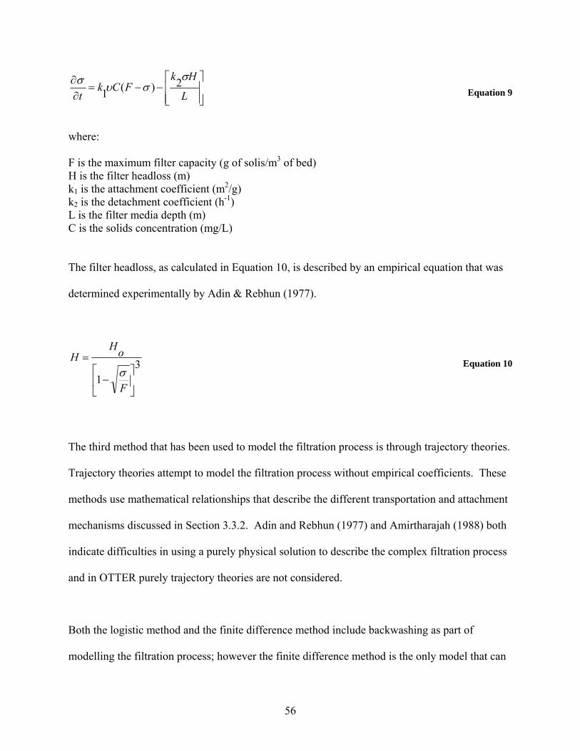
56
⎥⎥⎦
⎤
⎢⎢⎣
⎡−−=
∂∂
L
HkFCk
t
σσυσ 2)(1
Equation 9
where:
F is the maximum filter capacity (g of solis/m3 of bed) H is the filter headloss (m) k1 is the attachment coefficient (m2/g) k2 is the detachment coefficient (h-1) L is the filter media depth (m) C is the solids concentration (mg/L)
The filter headloss, as calculated in Equation 10, is described by an empirical equation that was
determined experimentally by Adin & Rebhun (1977).
31 ⎥
⎦
⎤⎢⎣
⎡−
=
F
oHH
σ
Equation 10
The third method that has been used to model the filtration process is through trajectory theories.
Trajectory theories attempt to model the filtration process without empirical coefficients. These
methods use mathematical relationships that describe the different transportation and attachment
mechanisms discussed in Section 3.3.2. Adin and Rebhun (1977) and Amirtharajah (1988) both
indicate difficulties in using a purely physical solution to describe the complex filtration process
and in OTTER purely trajectory theories are not considered.
Both the logistic method and the finite difference method include backwashing as part of
modelling the filtration process; however the finite difference method is the only model that can

57
be used to look at the affects of backwashing directly (WRc plc, 2002). The finite difference
model uses a backwashing model from Amirtharajah (1985) to model the process. The logistic
method, however, resets the filter to its original state after a backwash is performed.
3.4 System for Analysis: Brantford Water Treatment Plant
3.4.1 System Description
The Brantford Water Treatment Plant (WTP) treats Grand River raw water taken from the
Holmedale Canal. The treatment process consists of screening, coagulation, sand ballasted
flocculation (US Filter Actiflo™), sedimentation, chlorination, filtration, chloramination and
fluoridation (City of Brantford, 2005). A schematic of the treatment plant layout can be seen in
Figure 3.5.

Figure 3.5: Schematic of the Brantford Water Treatment Plant as of May 1999 (City of Brantford, 2006)
58
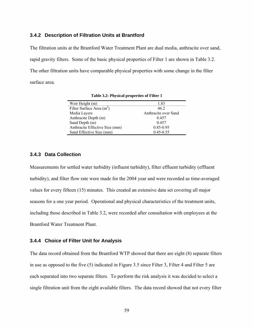
59
3.4.2 Description of Filtration Units at Brantford
The filtration units at the Brantford Water Treatment Plant are dual media, anthracite over sand,
rapid gravity filters. Some of the basic physical properties of Filter 1 are shown in Table 3.2.
The other filtration units have comparable physical properties with some change in the filter
surface area.
Table 3.2: Physical properties of Filter 1
Weir Height (m) 1.83 Filter Surface Area (m2) 46.2 Media Layers Anthracite over Sand Anthracite Depth (m) 0.457 Sand Depth (m) 0.457 Anthracite Effective Size (mm) 0.85-0.95 Sand Effective Size (mm) 0.45-0.55
3.4.3 Data Collection
Measurements for settled water turbidity (influent turbidity), filter effluent turbidity (effluent
turbidity), and filter flow rate were made for the 2004 year and were recorded as time-averaged
values for every fifteen (15) minutes. This created an extensive data set covering all major
seasons for a one year period. Operational and physical characteristics of the treatment units,
including those described in Table 3.2, were recorded after consultation with employees at the
Brantford Water Treatment Plant.
3.4.4 Choice of Filter Unit for Analysis
The data record obtained from the Brantford WTP showed that there are eight (8) separate filters
in use as opposed to the five (5) indicated in Figure 3.5 since Filter 3, Filter 4 and Filter 5 are
each separated into two separate filters. To perform the risk analysis it was decided to select a
single filtration unit from the eight available filters. The data record showed that not every filter
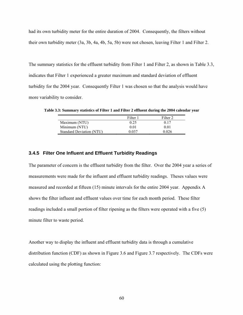
60
had its own turbidity meter for the entire duration of 2004. Consequently, the filters without
their own turbidity meter (3a, 3b, 4a, 4b, 5a, 5b) were not chosen, leaving Filter 1 and Filter 2.
The summary statistics for the effluent turbidity from Filter 1 and Filter 2, as shown in Table 3.3,
indicates that Filter 1 experienced a greater maximum and standard deviation of effluent
turbidity for the 2004 year. Consequently Filter 1 was chosen so that the analysis would have
more variability to consider.
Table 3.3: Summary statistics of Filter 1 and Filter 2 effluent during the 2004 calendar year
Filter 1 Filter 2 Maximum (NTU) 0.25 0.17 Minimum (NTU) 0.01 0.01 Standard Deviation (NTU) 0.037 0.026
3.4.5 Filter One Influent and Effluent Turbidity Readings
The parameter of concern is the effluent turbidity from the filter. Over the 2004 year a series of
measurements were made for the influent and effluent turbidity readings. Theses values were
measured and recorded at fifteen (15) minute intervals for the entire 2004 year. Appendix A
shows the filter influent and effluent values over time for each month period. These filter
readings included a small portion of filter ripening as the filters were operated with a five (5)
minute filter to waste period.
Another way to display the influent and effluent turbidity data is through a cumulative
distribution function (CDF) as shown in Figure 3.6 and Figure 3.7 respectively. The CDFs were
calculated using the plotting function:

61
( )1+ni
Equation 11
where
i is the plotting point of interest n is the number of plotting points
0.00
0.10
0.20
0.30
0.40
0.50
0.60
0.70
0.80
0.90
1.00
0 1 2 3 4 5 6 7 8 9 10
Filter Influent (NTU)
Cum
ulat
ive
Prob
abili
ty (P
i)
95 Percentile
Figure 3.6: Filter 1 influent turbidity cumulative distribution function for turbidity data during the 2004
calendar year
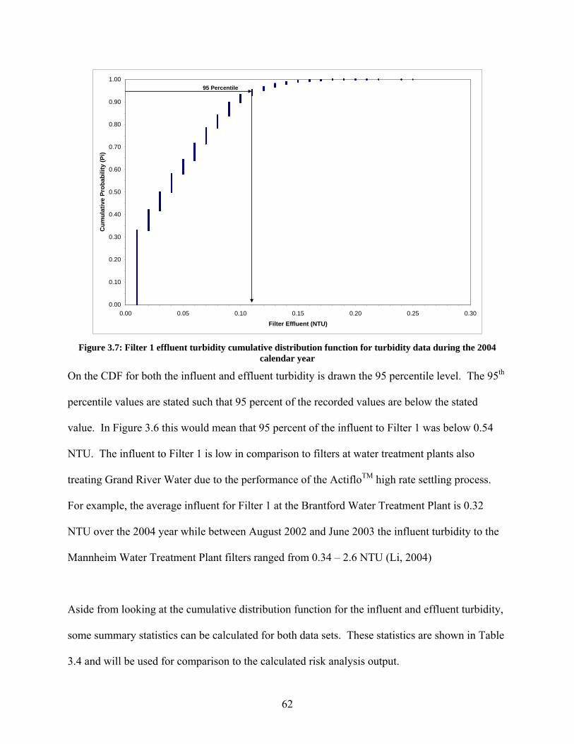
62
0.00
0.10
0.20
0.30
0.40
0.50
0.60
0.70
0.80
0.90
1.00
0.00 0.05 0.10 0.15 0.20 0.25 0.30
Filter Effluent (NTU)
Cum
ulat
ive
Prob
abili
ty (P
i)
95 Percentile
Figure 3.7: Filter 1 effluent turbidity cumulative distribution function for turbidity data during the 2004
calendar year
On the CDF for both the influent and effluent turbidity is drawn the 95 percentile level. The 95th
percentile values are stated such that 95 percent of the recorded values are below the stated
value. In Figure 3.6 this would mean that 95 percent of the influent to Filter 1 was below 0.54
NTU. The influent to Filter 1 is low in comparison to filters at water treatment plants also
treating Grand River Water due to the performance of the ActifloTM high rate settling process.
For example, the average influent for Filter 1 at the Brantford Water Treatment Plant is 0.32
NTU over the 2004 year while between August 2002 and June 2003 the influent turbidity to the
Mannheim Water Treatment Plant filters ranged from 0.34 – 2.6 NTU (Li, 2004)
Aside from looking at the cumulative distribution function for the influent and effluent turbidity,
some summary statistics can be calculated for both data sets. These statistics are shown in Table
3.4 and will be used for comparison to the calculated risk analysis output.
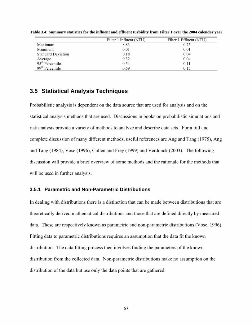
63
Table 3.4: Summary statistics for the influent and effluent turbidity from Filter 1 over the 2004 calendar year
Filter 1 Influent (NTU) Filter 1 Effluent (NTU) Maximum 8.83 0.25 Minimum 0.01 0.01 Standard Deviation 0.18 0.04 Average 0.32 0.04 95th Percentile 0.54 0.11 99th Percentile 0.69 0.15
3.5 Statistical Analysis Techniques
Probabilistic analysis is dependent on the data source that are used for analysis and on the
statistical analysis methods that are used. Discussions in books on probabilistic simulations and
risk analysis provide a variety of methods to analyze and describe data sets. For a full and
complete discussion of many different methods, useful references are Ang and Tang (1975), Ang
and Tang (1984), Vose (1996), Cullen and Frey (1999) and Verdonck (2003). The following
discussion will provide a brief overview of some methods and the rationale for the methods that
will be used in further analysis.
3.5.1 Parametric and Non-Parametric Distributions
In dealing with distributions there is a distinction that can be made between distributions that are
theoretically derived mathematical distributions and those that are defined directly by measured
data. These are respectively known as parametric and non-parametric distributions (Vose, 1996).
Fitting data to parametric distributions requires an assumption that the data fit the known
distribution. The data fitting process then involves finding the parameters of the known
distribution from the collected data. Non-parametric distributions make no assumption on the
distribution of the data but use only the data points that are gathered.

64
Vose (1996) strongly recommends using non-parametric distributions, but other authors such as
Verdonck (2003) provide no rule as to when to use one method over the other. However, Vose
(1996) also states that the use of parametric distributions is allowable if there is evidence to
suggest that the data are actually from the underlying theoretical distribution. There has been
some indication that water quality parameters follow parametric distributions such as the
lognormal distribution (Novotny, 2004). Therefore because of precedent and the simplicity of
their use, any future analysis will use parametric distribution fitting techniques. It is important to
note that the use of parametric or non-parametric methods can have a bearing on the final risk
result (Verdonck, 2003).
3.5.2 Theoretical Distributions
To use parametric distributions it is necessary to determine what theoretical distribution best
represents the measured data set. This is necessary as the distributional form can have a large
effect on the outcome of a risk assessment, especially in situations where the relative standard
deviation, the ratio of the standard deviation to the mean, is greater than one (Haas, 1997).
There are a wide range of parametric distributions that the data set can be fitted to. Some of
them are the exponential, gamma, lognormal, normal, Weibull, and Gumbel (Vose, 1996). It
was decided to perform distribution fitting techniques on four (4) common distributions namely
the normal, lognormal, exponential, and Gumbel distribution. The lognormal and normal
distributions were chosen because natural data tends to follow these distributions (Vose, 1996).
The lognormal distribution has been used to model naturally occurring data by Eisenberg et al.
(1998) while the normal distribution was used by Sadiq et al. (2003) to model filtration rate, even
thought it was indicated that the normal distribution was used arbitrarily. The Gumbel

65
distribution is an extreme value distribution and the exponential distribution is based on times for
an occurrence of an event (Vose, 1996). These distributions are included in the analysis to cover
a range of possible distributions and because extreme value distributions have been used to
model removal efficiencies, such as the removal efficiency of a slow sand filter for total
coliforms (Saidq et al., 2003). For the lognormal distribution, it is possible to use either the
common lognormal, base 10, or the Napierian lognormal, base e, distribution. The logarithmic
base 10 distribution was used because Novotny (2004) states that water quality measurements
may often follow lognormal (base 10) distributions and because both base 10 and base e
distributions are similar (Burmaster & Hull, 1997).
3.5.3 Parameter Estimation Methods
To determine which of the theoretical distributions best represents the data set, it is necessary to
determine the numerical values for the parameters that describe an each assumed distribution.
There are different parameter estimation methods for parametric and non-parametric
distributions; however, since the analysis will focus on parametric distributions, only parameter
estimation methods for parametric distributions will be discussed here. Further discussion on
both parametric and non-parametric distributions can be seen in Cullen and Frey (1999), Vose
(1996) and Verdonck (2003). Three of the most common techniques for parameter estimation
are the method of moments, the probability plotting method and the method of Maximum
Likelihood. Ang and Tang (1975) and Vose (1996) provide a good description of the different
methods and a mathematical reason for their use.
66
3.5.3.1 Method of Matching Moments
For any given data set, statistical values such as the mean, standard deviation and kurtosis can be
calculated. These values are known as the moments of the data set where the mean is the first
moment, standard deviation is the second moment, and kurtosis is the third moment.
Any distribution is described by a set of parameters. For example the normal distribution is
described by µ and σ and the exponential distribution is described by µ and β. The moments
of the data set have a relationship to the parameters of the distribution, so to determine the
parameters of the distribution it is possible to first determine the moments of the data set and
then calculate the parameters of the distribution. Table 3.5 shows some of the relationships
between the moments of the data set and the parameters of some common distributions. In Table
3.5, E(x) represents the mean and Var(x) represents the variance of the data set.

Table 3.5: Relationship between distribution parameters and the mean and variance of a measured data set (adapted from Ang & Tang, 1975)
Distribution Probability Density Function (PDF) Parameters Relation to Mean and Variance*
Normal
⎥⎥⎦
⎤
⎢⎢⎣
⎡⎟⎠⎞
⎜⎝⎛ −
−=2
21exp
21
σµx
πσfx(x)
σ µ
E(X) = µ Var(X) = σ2
Lognormal
⎥⎥
⎦
⎤
⎢⎢
⎣
⎡⎟⎠
⎞⎜⎝
⎛ −−=
2ln21exp
21
ξλx
πxξfx(x)
λ ξ
E(X) = exp(λ + ½ζ2)
Var (X) = ⎥⎥⎦
⎤
⎢⎢⎣
⎡−1
22 ξe(X)E
Exponential β
µ
β
)(
e1f(x)
−−
=
x
µ β
E(X) = β + µ Var (X) =β2
Gumbel β
µ)(x
ee
x
ef(x)
−−
−−
−= β
µ
β
)(1
µ β
E(X) = µ + 0.5772β
Var(X) = 2
6 ⎟⎟⎠
⎞⎜⎜⎝
⎛ β*π
* E(X) represents the mean and Var(X) represents the variance
67

68
3.5.3.2 Probability Plotting Method
The probability plotting method plots the measured data set and the cumulative probability on
specially constructed probability paper (Cullen & Fery, 1999). Probability paper is constructed
so that if the measured data set is from the assumed distribution the plot is a straight line.
Every probability distribution has a cumulative distribution equation described as F(x) = some
function of x where F(x) is the cumulative distribution of the measured data and x is some
measured data point. The measured data is sorted in increasing order and then ranked from one
(1) to N where N is the number of data points. The plotting position is then calculated using a
plotting position equation such as m/(N+1) where m is the ranked number and N is the number
of data points. This numerical value is then the plotting position for that measured data point and
the combination of all the plotting position points is the cumulative distribution function, F(x),
for the measured data.
When using probability plotting, the cumulative distribution function is convoluted such that it is
represented as x = some function of F(x) (Pandey, 2004). Then the data is plotted with x on one
axis and the function of F(x) is plotted on the other axis. Through plotting, the slope and y-
intercept can be calculated for the constructed line. These values are then used to determine the
parameters of the distribution. It should be noted that as the number of parameters in a
distribution increases to three or more, the number of dimensions for a probability plot would
have to correspondingly increase. An example for the Gumbel distribution is provided below.
The cumulative distribution function for the Gumbel distribution is

69
βµ)(x
eeF(x)
−−
−=
Equation 12
After convolution the equation can be represented as
[ ] µβ +−−= )))(ln(ln( xFx Equation 13
Therefore, the data set is plotted as x (y-axis) vs [ ]))(ln(ln xF− where F(x) is described by the
plotting position of x. From plotting the data the slope and y-intercept can be determined.
Relating the slope and y-intercept back to Equation 13, β− is the slope and µ is the y-
intercept, which are the parameters of the Gumbel distribution.
3.5.3.3 Method of Maximum Likelihood
The method of Maximum Likelihood looks to determine the parameters of the distribution that
are most likely to give the observed data set. To determine the parameters of the distribution, a
likelihood function is calculated which describes how likely it is that a given parameter value
produces the measured data set.
The likelihood function is (Cullen and Frey, 1999):
∏=
=n
i kixfkL1
),...,2,1/(),...,2,1( θθθθθθ
Equation 14
where:
L is the likelihood function θ1, θ2,… θk are the parameters of the probability distribution n is the total number of data points in the measure data record

70
The best estimate of the values of the parameters is then determined by maximizing the
likelihood function using a maximization methodology such as differentiation or Taylor series
expansion.
3.5.3.4 Comparison of Parameter Estimation Methods
Although the above methods are all parameter estimation methods, the parameters calculated
from the different methods are not always the same. Vose (1996) recommends using the
Maximum Likelihood method but also acknowledges that the Maximum Likelihood method is
sometimes difficult to implement and that one method is not always the best method.
Vose (1996) also indicates that if the coefficient of determination is high (0.90 or 0.95) for the
straight line in the probability plotting method, the method of moments and the probability
plotting method provide similar results. Cullen and Frey (1999) acknowledge that the method of
moments is the most straightforward and practical method to implement. For future analysis the
method of moments will be used primarily for simplicity. However, any risk analysis should be
performed with the understanding that differences between the methods are possible.
3.5.4 Selecting a Theoretical Distribution
After determining the parameters for the different possible distributions, it is necessary to
determine which of the distributions best represents the measured data set. To perform this
analysis probability plotting will be used both to calculate an r2 parameter and to provide a visual
comparison of the degree to which the different distributions fit the data set. The r2 parameter is
defined as the coefficient of multiple determination. This parameter will be used to determine

71
how well the measured data matches the assumed model, with 1 being a perfect match and 0
being no match at all.
3.5.4.1 Probability Plotting
Section 3.5.3.2 outlines the construction of probability plots and their use to undertake parameter
estimation. Another use of probability plotting is with determining the goodness of fit of an
assumed distribution to the data set. The construction of a probability plot allows for the
linearity of the graph to be used as an evaluation mechanism for the goodness of fit for a
distribution (Ang & Tang, 1975). Therefore, for a two-dimensional probability plot, the r2 value
of the trend line provides a useful comparison value for different assumed distributions. Since r2
is a measure of the degree to which a line represents the data, a larger r2 number provides a
stronger indication that the data set follows the assumed distribution. Furthermore, this
comparison can be performed visually.
3.5.5 Probabilistic Risk Assessment, Variability and Uncertainty
The nature of probabilistic risk assessments allows for a greater characterization of the
variability and uncertainty in a population, and consequently a determination of the variability
and uncertainty in a given risk.
Variability can be described as naturally occurring differences in a parameter while uncertainty
is lack of knowledge in that parameter (Cullen & Frey, 1999). So while uncertainty can be
reduced through further sampling, variability cannot. However, both variability and uncertainty
are properties of their respective sampled populations and must be incorporated into a final risk

72
estimate (Verdonck, 2003). The use of simulation techniques allows for both variability and
uncertainty to be taken into account during a risk assessment.
3.5.6 Simulation Techniques
There are a variety of numerical simulation techniques that can be used during a risk analysis
including Monte Carlo simulation, Latin Hypercube Sampling, and Importance Sampling (Cullen
& Frey, 1999). Monte Carlo simulation, discussed in more detail in Sections 3.5.6.1 to 3.5.6.3,
provides completely random sampling of the parent distribution or data set to generate inputs to
the model. Latin Hypercube Sampling reduces the number of simulations necessary by
separating the original distribution into percentiles of equal probability and one sample is taken
from each percentile (Cullen & Frey, 1999). This has the effect of reducing the overall number
of simulations necessary. Importance Sampling focuses the sampling on a defined area of
importance. Thus this method is useful for looking at specific parts of a distribution, such as the
tails, but not at a distribution as a whole (Cullen & Frey, 1999).
The Monte Carlo technique will be used for future analysis because it is commonly used and thus
easily understood, is not dependent on a set of assumptions about the nature of the variability and
uncertainty, and is able to deal with both uncertainty and variability either separately or together
(Verdonck, 2003).
3.5.6.1 Monte Carlo Analysis
The Monte Carlo simulation technique, developed in the 1940’s, was originally used to solve
complex mathematical integration problems (Cullen & Frey, 1999). Monte Carlo analysis
73
involves running a model repeatedly while constantly changing the input values which are
chosen randomly from their overall parent distributions.
This analysis generates a set of output values that characterize different possible outcomes. For a
more comprehensive description of the Monte Carlo simulation technique see Cullen and Frey
(1999).
3.5.6.2 First Order Monte Carlo Analysis
A first order Monte Carlo analysis is another name for what is usually described as a Monte
Carlo analysis. The distinction is made here because of the following discussion on second order
Monte Carlo analysis. First order Monte Carlo analysis makes no distinction between
uncertainty and variability (Verdonck, 2003). Input variables are assumed to be completely
characterized by the assumed “best fit” distribution and the values of the parameters of that
distribution. During first order Monte Carlo analysis, a random value is chosen from the
distribution and run through the model.
3.5.6.3 Second Order Monte Carlo Analysis
In a Second Order Monte Carlo analysis, uncertainty and variability are separated (Verdonck,
2003). A second order Monte Carlo analysis recognizes that the values of the parameters
calculated for the chosen distribution are based on a data set that may be incomplete. Therefore
the values of the parameters are considered to vary within a range specified by confidence limits.
The simulation procedure then uses a looped technique to account for both the variability in the
data set, captured by the distribution, and the uncertainty in the parameters of the distribution
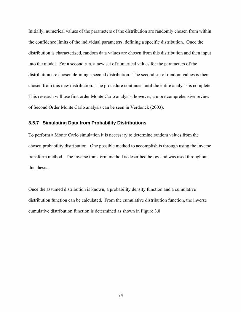
74
Initially, numerical values of the parameters of the distribution are randomly chosen from within
the confidence limits of the individual parameters, defining a specific distribution. Once the
distribution is characterized, random data values are chosen from this distribution and then input
into the model. For a second run, a new set of numerical values for the parameters of the
distribution are chosen defining a second distribution. The second set of random values is then
chosen from this new distribution. The procedure continues until the entire analysis is complete.
This research will use first order Monte Carlo analysis; however, a more comprehensive review
of Second Order Monte Carlo analysis can be seen in Verdonck (2003).
3.5.7 Simulating Data from Probability Distributions
To perform a Monte Carlo simulation it is necessary to determine random values from the
chosen probability distribution. One possible method to accomplish is through using the inverse
transform method. The inverse transform method is described below and was used throughout
this thesis.
Once the assumed distribution is known, a probability density function and a cumulative
distribution function can be calculated. From the cumulative distribution function, the inverse
cumulative distribution function is determined as shown in Figure 3.8.

75
Figure 3.8: Construction of the inverse cumulative distribution function (Frey, 1992)
To choose a random data point from the assumed distribution, a random number ranging from
zero (0) to one (1) is chosen from a uniform distribution. This random value is then input into
the inverse cumulative distribution function to determine a random value from the original
distribution. This procedure is shown in Figure 3.9.
Probabiliy Density Function
Value of Random Variable, x
Prob
abili
y D
ensi
tyCumulative Distribution Function
0
1
Value of Random Variable, x
Cum
ulat
ive
Prob
abili
ty
Inverse Cumulative Distribution Function
0 1
Cumulative Probability
Valu
e of
Ran
dom
Var
iabl
e, x

76
Figure 3.9: Inverse transform method
The inverse transform method is performed repeatedly until the total number of random data
points needed for analysis is determined.
3.5.8 Random Number Generation
In order to simulate data from probability distributions using the inverse transform method, as
described in Section 3.5.7, a random number must be generated. Therefore, it is necessary to
construct a random number generator.
Inverse Cumulative Distribution Function
0 1
Cumulative Probability
Valu
e of
Ran
dom
Var
iabl
e, x
Uniform Distribution
0
1
0 1
Value of Random Variable, x
Prob
abili
ty D
ensi
ty

77
The research in this thesis will not focus on determining a new random number generator but
will use generators that are currently available. One of these is the built in random number
generator in Microsoft Excel 2002 and Microsoft Excel 2003. The use of Microsoft Excel 2002
for statistical analysis of data and specifically for the use of the random number generator is
cautioned by McCullough and Wilson (2002). One of the errors noted by McCullough and
Wilson (2002) is that Microsoft Excel 2002 returns highly improbable random values too
frequently to be correct from a probabilistic perspective. Through an analysis of Microsoft Excel
2003 by McCullough and Wilson (2005) it was shown that this flaw was resolved for the RND
function. However, McCullough and Wilson (2005) still indicate a number of flaws with the
random number generator in Microsoft Excel 2003. Although the errors within the random
number generator in Microsoft Excel 2003 are well documented, this random number generator
will be used throughout this thesis. It is important to note that statistical errors are possible and
that a more detailed analysis should use a random number generator that satisfies all statistical
tests. Law and Kelton (1991) describe a series of different random number generators, along
with some common problems with random number generators and methods of testing random
number generators
3.5.9 Correlated Water Quality Parameters
If a risk analysis requires that a data set be generated for two or more incoming variables the
concept of correlation becomes important. Correlation is the degree that one variable is related
to another (Verdonck, 2003). As an example, for incoming water quality variables, this could
mean that the microbial count in a water source varies directly with the temperature of the water.
Performing a simple Monte Carlo simulation on these two variables would choose a random
value of the microbial count independently of the temperature. Since the two variables are

78
correlated, the assumption of independence is incorrect. Therefore, a method that takes into
account the correlations between the parameters would be necessary in this situation.
The method of Iman and Canover (1982) is one method that has been developed to deal with
correlated variables. This method was developed in a way that several different parameter
distributions can be combined together (Haas, 1999). Restricted pairing techniques, described by
Cullen and Frey (1999), are another method for dealing with correlated variables. This method
works when there is an independent distribution which has any number of dependent
distributions. A value is sampled from the independent distribution, and then based on the value
of the independent variable, the distribution of the dependant variable can be determined. A
value from the new dependent distribution is then calculated.
The risk analysis methodology used to calculate the risk of producing non-compliant water will
not consider correlated incoming variables. However the importance of correlations in risk
assessments is shown by Burmaster and Anderson (1994) who, as one of their fourteen principles
of good practice for conducting a Monte Carlo risk assessment, state that all moderate or strong
correlations between parameters should be taken into account. It is therefore recommended that
any detailed risk analyses take into account correlated variables.
3.6 Summary of Analysis Methodologies
After choosing the different statistical and probabilistic techniques that will be used throughout
the analysis, the final water treatment plant risk analysis methodologies can be re-stated
incorporating the different factors previously determined.

79
3.6.1 Summary of CFA Methodology
3.6.1.1 Step 1: Define Water Treatment Plant
For the CFA methodology defining the water treatment plant involves deciding which treatment
processes with the treatment plant to analyze. During this process a schematic of the treatment
unit or units that are analyzed should be drawn. For the risk analysis performed in this study, the
treatment process of interest is a dual media rapid gravity filtration unit.
3.6.1.2 Step 2: Determine Parameters to Analyze
The different parameters that will be used in the CFA should be determined. Although a large
number of parameters would give a better picture of the overall operation of the treatment unit or
plant, as the number of parameters increase the amount of time and data needed for an analysis
increases as well. Currently there are no guidelines to determine what parameters to choose, but
the choice will be a function of expert knowledge from both the water treatment plant operator
and the risk analyst. The CFA of the filter in this study focused on turbidity as the parameter of
concern.
3.6.1.3 Step 3: Determine the Influent Water Quality and the Percent Removal
Distributions
Using the method of moments the theoretical distribution parameters can determined. Then
using probability plotting and visual inspection of probability plots, the best fitting distribution
can be determined. This study requires that the probability distribution of the influent turbidity
and the percentage reduction of turbidity across the filtration unit be determined.

80
3.6.1.4 Step 4: Perform Monte Carlo Simulation
Using first order Monte Carlo simulation, a random influent value will be chosen from the
influent distribution and a random percent reduction value will be chosen from the percent
removal distribution. These two values will be multiplied together and recorded as the simulated
effluent distribution. This overall process will be performed a number of times to take into
account a large number of possible combinations of influent water quality and percent reduction.
The relationship between influent turbidity concentration and the percent removal of turbidity
across the filter was analyzed later on in this thesis to see whether or not the percent removal of
turbidity is independent of the influent turbidity concentration.
3.6.1.5 Step 5: State Conclusions
For each parameter that is chosen in Step 2, a risk level can be generated. This information can
then be presented to managers and operators allowing for solutions to lower either overall risk or
the risk associated with one specific parameter.
3.6.2 Summary of the Risk Analysis Method which Combines Computer
Modelling and Probabilistic Risk Analysis
3.6.2.1 Step 1: Define Water Treatment Plant and Set-Up Model
This step involves collecting the physical data that characterizes the system that will be analyzed
and incorporating it into the computer model. For this study, the number of filters, size of filters,
and other data describing the filtration process was recorded. This data was then used to
accurately depict the water treatment process within the model.

81
3.6.2.2 Step 2: Determine Parameters to Analyze
This step is important from a risk analysis perspective. A greater number of parameters analyzed
will increase the precision of the risk analysis results, but could also increase the computational
time and difficulty. Currently there are no guidelines to determine what parameters to choose,
but the choice will be a function of expert knowledge from both the water treatment plant
operator and the risk analyst. The analysis of the filtration unit focused on turbidity as the
parameter of concern.
3.6.2.3 Step 3: Calibrate the Computer Model
The calibration step is necessary to ensure accurate prediction results from the model. The
procedures for calibration should follow those described for the different process models with
the modelling software.
3.6.2.4 Step 4: Determine Distributions of Water Quality Parameters
Using the method of moments the theoretical distribution parameters can determined. Then
using probability plotting and visual inspection of probability plots, the best fitting distribution
that describes the water quality parameters can be determined. This analysis required that the
influent turbidity and filter flow rate distributions be determined.
3.6.2.5 Step 5: Simulate Incoming Water Quality Data
Using a random number generator and the inverse transform method, input data can be
determined. Initially a First-Order Monte Carlo simulation was done, so it was assumed that the
parameters of the distribution calculated in Step 4 are correct. For the analysis of the filtration
unit, the input turbidity and input filter flow rate were simulated. Since only one parameter was
considered in this thesis, that of turbidity, correlation between incoming water quality parameters

82
was not taken into account. However, a more comprehensive study which incorporates multiple
parameters should look at the correlation between the influent water quality variables.
3.6.2.6 Step 6: Run Calibrated Model with Simulated Data
Once the raw water quality data have been simulated, the data is entered into the model. The
model will be run for the data series and the output stored. This output can then be represented
as a cumulative distribution function where the percent time that the data is less than a given
level can be determined.
3.6.2.7 Step 7: State Conclusions
For each parameter that is chosen in Step 2, a risk level can be generated. This information can
then be presented to managers and operators allowing for solutions to lower either overall risk or
the risk associated with one specific parameter.

83
CHAPTER 4 RESULTS AND DISCUSSION USING THE CONSEQUENCE FREQUENCY ASSESSMENT
4.1 Application of CFA Methodology to Filter 1
The consequence frequency assessment was used on Filter 1 of the Brantford Water Treatment
Plant. To perform this analysis, it was necessary to take the principles of the CFA and directly
apply them to a rapid gravity filtration unit, a process that is depicted in Figure 4.1.

84
Figure 4.1: Diagram of CFA methodology applied to filtration unit
The influent turbidity (C0) is represented as a probability distribution function (PDF) and the
rapid gravity filter is modelled as a percent reduction PDF (C1/C0) The CFA methodology
multiples a randomly selected value from the influent turbidity PDF by a randomly selected
value from the percent reduction PDF to give a possible output value for the filter (C2). After a
PDF of Percent Reduction (C1 /C0)
Simulated CDF of Output (C2)
PDF of Influent Turbidity (Co)
Filtration Process
CFA Simulation of the Filtration Process
20
1 CC
CoC =⎟
⎟
⎠
⎞
⎜⎜
⎝
⎛
Rapid Gravity Filter (C1/C0)Turbidity Influent (C0)
Turbidity Effluent (C1)

85
number of simulations, all the possible effluent turbidity values (C2) that are calculated can be
represented as a cumulative distribution function (CDF) of the effluent turbidity.
4.1.1 Data Manipulation for Percent Reduction Calculation
Percent reduction is calculated by (influent-effluent)/influent. This calculation was performed
for every data point over the 2004 year data record. A percentage reduction was not calculated
when data were missing or not available from either the influent or effluent turbidity data record.
In some situations the percent reduction was not able to be calculated because the influent values
were “0”, causing the percent reduction value to be a non-integer. In these conditions a percent
reduction was not recorded. An example of this occurrence is on July 25, 2004 from 10:00 am to
11:30 am. A further complication occurred when the percentage reduction values were negative,
indicating that the effluent turbidity was greater than the influent turbidity. One example is on
July 25, 2004 at 9:45 AM another on July 25, 2004 at 11:45 am. The influent turbidity values
are 0.01 and 0.02 NTU respectively in these cases, while the effluent turbidity is around 0.60
NTU. During the analysis, the data was not offset to account for contact time in the process;
however, as the use of the data was for risk analysis and the data set was large it was assumed
that this assumption would have a negligible impact. Future analysis should check this
assumption.
It was decided to keep all the data points, including those that gave a negative percentage
reduction, since it is possible for a filter to experience detachment if captured particles are
sloughed from the filter media (MWH, 2005). However, if negative percentage removal values
were included, the lognormal distribution could not be used to model the process, as negative

86
values are incompatible with the lognormal distribution. Thus, to use the lognormal distribution,
a value of percent remaining as opposed to percent reduction was used. Using the percent of
influent turbidity remaining in the effluent eliminated the negative values within the data record
but still allowed for the effluent to be greater than the influent (Dunn, Frodsham, & Kilroy,
1998).
After performing the necessary calculations, a CDF for the percentage of influent turbidity
remaining was determined. This CDF is shown in Figure 4.2, while summary statistics for the
percentage of influent turbidity remaining can be seen in Table 4.1.
0.00
0.10
0.20
0.30
0.40
0.50
0.60
0.70
0.80
0.90
1.00
0 100 200 300 400 500 600
Percent Remaining (%)
Cum
ulat
ive
Prob
abili
ty (P
i)
95 Percentile
Figure 4.2: Cumulative distribution function of the percentage of influent turbidity remaining for filter 1

87
Table 4.1: Summary statistics for the percentage of influent turbidity remaining for filter 1
Percent of Influent Turbidity Remaining (%)
Maximum (%) 500 Minimum (%) 0.4 Average (%) 14.8 Standard Deviation (%) 13.0 95th Percentile (%) 40.0 99th Percentile (%) 56.3
4.1.2 Distribution Fitting of Data
In order to perform the CFA, a distribution fitting process was undertaken to determine the
probability distribution functions for the influent turbidity and the percent of influent turbidity
remaining. This process follows the procedure that was described in Section 3.5.3 and Section
3.5.4.
Initially the method of moments was used to obtain the distribution parameters for the four
selected distributions. These parameters were then used to characterize the four different
distributions when undertaking the distribution fitting exercise. Table 4.2 and Table 4.3 outline
the distribution fitting comparison parameters while Figure 4.3, and Figure 4.4 provide a visual
comparison of the distribution fitting process. For a visual comparison, the closer the data points
plot to a straight line, the better the assumed distribution fits the data set.
Table 4.2: Distribution fitting statistics for influent turbidity
Probability Plotting (r2) Normal 0.613 Lognormal 0.964 Exponential 0.712 Gumbel 0.708

88
Table 4.3: Distribution fitting statistics for percentage of influent turbidity remaining
Probability Plotting (r2) Normal 0.807 Lognormal 0.963 Exponential 0.965 Gumbel 0.938
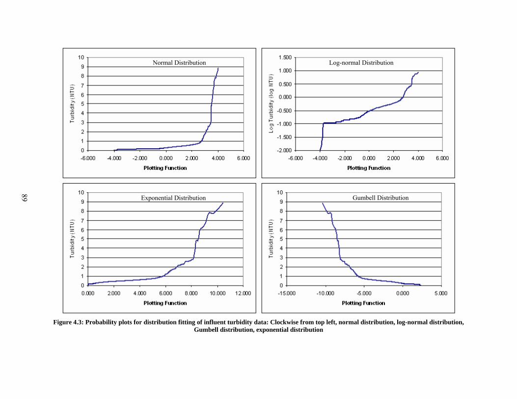
Figure 4.3: Probability plots for distribution fitting of influent turbidity data: Clockwise from top left, normal distribution, log-normal distribution,
Gumbell distribution, exponential distribution
89
Normal Distribution Log-normal Distribution
Exponential Distribution Gumbell Distribution

Figure 4.4: Probability plots for distribution fitting of the percent of influent turbidity remaining data: Clockwise from top left, normal distribution, log-normal distribution, Gumbell distribution, exponential distribution
90
Normal Distribution Log-normal Distribution
Exponential Distribution Gumbell Distribution

91
From Table 4.2 and Table 4.3 it can be seen that the lognormal distribution provides the best fit
to both the influent turbidity and the percentage of influent turbidity remaining data. From this
analysis it was decided that the lognormal distribution would be used for future analysis. Table
4.4 shows the final distribution parameters for the lognormal distribution.
Table 4.4: Lognormal distribution parameters for influent turbidity and percentage of turbidity remaining
Influent Turbidity (NTU)
Percentage of Influent Turbidity Remaining (%)
µ -0.54 -0.98 σ 0.19 0.37
4.1.3 Simulation Convergence
To determine the outcome of any simulation, the issue of simulation convergence, also referred
to as numerical stability, is important. Burmaster and Anderson (1994) stated, as principle
twelve of their fourteen principles of good practice in the use of Monte Carlo simulation
techniques, that the numerical stability of a simulation must be investigated. One method of
investigating the convergence of a simulation is through plotting the output from a simulation as
a function of the number of shots performed during the simulation (Verdonck, 2003). A shot is
one calculation and a simulation is the entire set of calculations. For each simulation different
percentile levels are calculated and tracked. Through tracking the percentile values for each
simulation, the convergence of the simulation can be seen. Percentile levels are calculated such
that x% of the output is below the stated level. For example, at the 95th percentile level, 95
percent of the output is below the stated value. Figure 4.5 and Figure 4.6 show the convergence
of the CFA simulation for the rapid gravity filtration unit.

92
0.00
0.02
0.04
0.06
0.08
0.10
0.12
0 20000 40000 60000 80000 100000 120000 140000 160000 180000 200000
Number of Shots
Efflu
ent T
urbi
dity
(NTU
)
10 Percentile50 Percentile80 Percentile90 Percentile
Figure 4.5: Convergence of the CFA simulation: 90th percentile and below
0.00
0.10
0.20
0.30
0.40
0.50
0.60
0.70
0 20000 40000 60000 80000 100000 120000 140000 160000 180000 200000
Number of Shots
Efflu
ent T
urbi
dity
(NTU
)
95 Percentile99 Percentile99.9 Percentile
Figure 4.6: Convergence of the CFA simulation: 95th percentile and above

93
Figure 4.5 and Figure 4.6 show that the CFA performed on the rapid gravity filtration unit
converges rapidly for low (10 – 50th) percentile levels (approximately 40,000 shots), as
illustrated in Figure 4.5; however, takes a while for the 95th and 99th percentiles to converge
(approximately 100,000 shots), as illustrated in Figure 4.6. For analysis purposes, the 99th
percentile is the highest percentile level to be used. Thus the slight undulation of the 99.9th
percentile is shown only to illustrate the difficulty that some simulations can have in stabilizing.
Furthermore, because the 99.9th percentile has not yet converged at 180,000 shots, the maximum
values recorded during a simulation at this number of shots should be used with extreme caution.
From the simulation convergence study, it was decided to use 180,000 shots per simulation for
all further CFA investigations since the 99th percentile and below have all converged by this
number of shots.
4.2 CFA Simulation Output
A full CFA was performed for 180,000 shots and can be seen in Figure 4.7. From the CFA
output, a set of summary statistics was calculated and compared to the actual effluent turbidity
experienced by the filtration unit for the 2004 year. Table 4.5 shows these values.

94
0.00
0.10
0.20
0.30
0.40
0.50
0.60
0.70
0.80
0.90
1.00
0.00 0.50 1.00 1.50 2.00 2.50 3.00 3.50
Effluent Turbidity (NTU)
Cum
ulat
ive
Prob
abili
ty (P
i)
Figure 4.7: Cumulative distribution function for a full CFA simulation
Table 4.5: Summary statistics of effluent turbidity for a full CFA simulation
Filter 1 Effluent (NTU) CFA Effluent (NTU) Maximum 0.25 2.92 Minimum 0.01 0.01 Standard Deviation 0.04 0.06 Average 0.04 0.05 95 Percentile 0.11 0.15 99 Percentile 0.15 0.28
The summary values from Table 4.5 show a discrepancy between what is currently experienced
by the filter and what could possibly occur according to the CFA. Although the minimum,
standard deviation and average turbidity values are similar, from a risk perspective, the
simulation results indicate that there is a greater probability of higher effluent turbidity water
being produced than what is currently experienced at the water treatment plant.

95
This increased probability of producing non-compliant water is illustrated by the increasing
divergence in effluent turbidity values between the simulated data and the measured data at
higher percentile levels, such as the 95th and 99th percentiles. For example, while the filtration
unit currently operates such that 99% of the effluent turbidity is below 0.15 NTU, the simulation
indicates that the filtration unit is operating such that 99% of the effluent turbidity is below 0.28
NTU. The divergence at the 99 percentile level amounts to a 0.13 NTU difference between the
simulated data and the measured data. While the different in the effluent turbidity level does not
seem large, this increase could have an effect on microbial contaminants as described in Huck et
al., 2001; Huck et al., 2002; and Emelko et al., 2003.
This divergence is shown visually in Figure 4.8 and Figure 4.9. Figure 4.9 is identical to Figure
4.8 but it concentrates on the percentile levels between 90 and 100 where the differences
between the two data series become more significant. The rest of the CDFs that will be
displayed throughout this thesis will only concentrate on the area of interest; however, Appendix
B displays the entire CDF for each graph shown.

96
0.00
0.20
0.40
0.60
0.80
1.00
0.00 0.50 1.00 1.50 2.00 2.50 3.00
Effluent Turbidity (NTU)
Cum
ulat
ive
Prob
abili
ty (P
i)
Measured EffluentCFA Simulated Effluent
Figure 4.8: Comparison between measured turbidity effluent and CFA simulated effluent
0.90
0.95
1.00
0.00 0.50 1.00 1.50 2.00 2.50 3.00
Effluent Turbidity (NTU)
Cum
ulat
ive
Prob
abili
ty (P
i)
MeasuredEffluent
CFA SimulatedEffluent
Figure 4.9: Comparison between measured turbidity effluent and CFA simulated effluent for a cumulative
probability of 90% and above
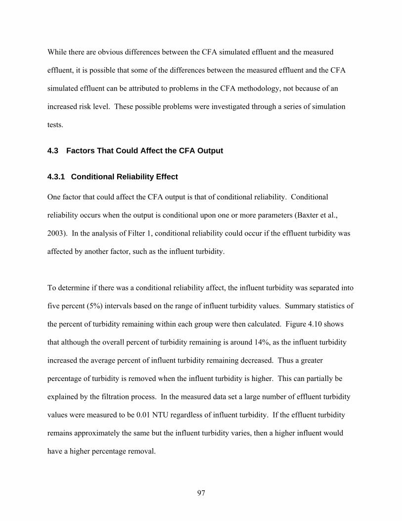
97
While there are obvious differences between the CFA simulated effluent and the measured
effluent, it is possible that some of the differences between the measured effluent and the CFA
simulated effluent can be attributed to problems in the CFA methodology, not because of an
increased risk level. These possible problems were investigated through a series of simulation
tests.
4.3 Factors That Could Affect the CFA Output
4.3.1 Conditional Reliability Effect
One factor that could affect the CFA output is that of conditional reliability. Conditional
reliability occurs when the output is conditional upon one or more parameters (Baxter et al.,
2003). In the analysis of Filter 1, conditional reliability could occur if the effluent turbidity was
affected by another factor, such as the influent turbidity.
To determine if there was a conditional reliability affect, the influent turbidity was separated into
five percent (5%) intervals based on the range of influent turbidity values. Summary statistics of
the percent of turbidity remaining within each group were then calculated. Figure 4.10 shows
that although the overall percent of turbidity remaining is around 14%, as the influent turbidity
increased the average percent of influent turbidity remaining decreased. Thus a greater
percentage of turbidity is removed when the influent turbidity is higher. This can partially be
explained by the filtration process. In the measured data set a large number of effluent turbidity
values were measured to be 0.01 NTU regardless of influent turbidity. If the effluent turbidity
remains approximately the same but the influent turbidity varies, then a higher influent would
have a higher percentage removal.
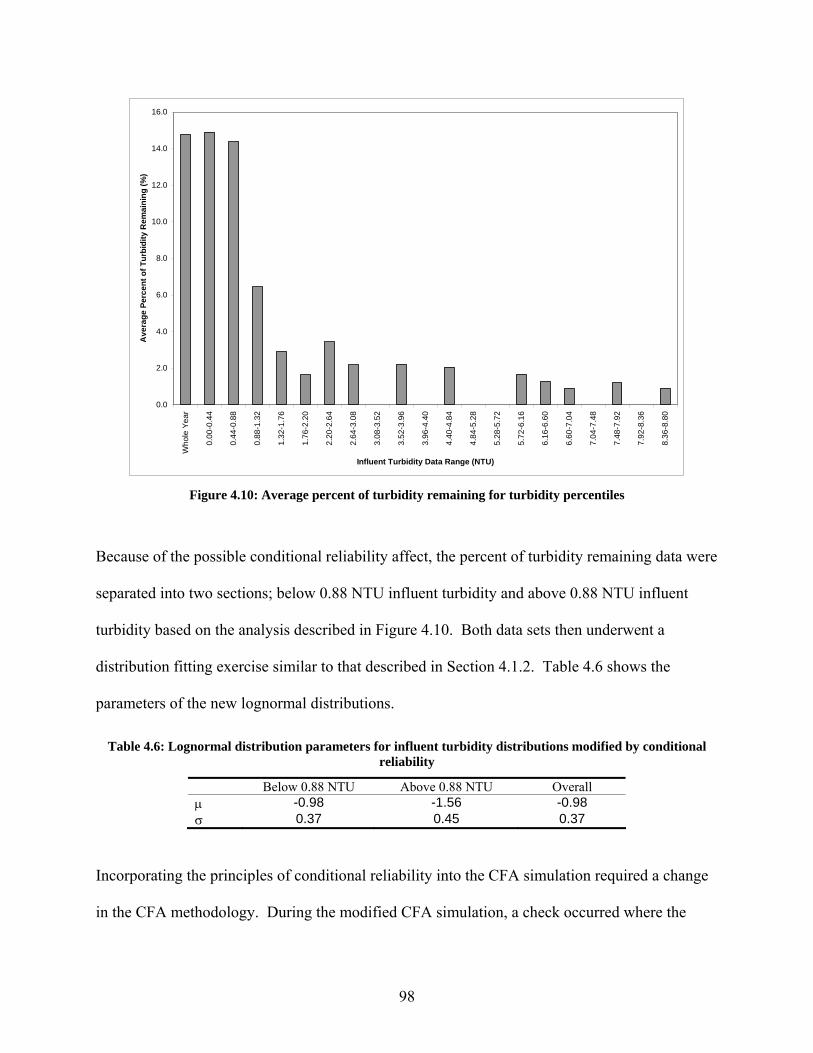
98
0.0
2.0
4.0
6.0
8.0
10.0
12.0
14.0
16.0
Who
le Y
ear
0.00
-0.4
4
0.44
-0.8
8
0.88
-1.3
2
1.32
-1.7
6
1.76
-2.2
0
2.20
-2.6
4
2.64
-3.0
8
3.08
-3.5
2
3.52
-3.9
6
3.96
-4.4
0
4.40
-4.8
4
4.84
-5.2
8
5.28
-5.7
2
5.72
-6.1
6
6.16
-6.6
0
6.60
-7.0
4
7.04
-7.4
8
7.48
-7.9
2
7.92
-8.3
6
8.36
-8.8
0
Influent Turbidity Data Range (NTU)
Ave
rage
Per
cent
of T
urbi
dity
Rem
aini
ng (%
)
Figure 4.10: Average percent of turbidity remaining for turbidity percentiles
Because of the possible conditional reliability affect, the percent of turbidity remaining data were
separated into two sections; below 0.88 NTU influent turbidity and above 0.88 NTU influent
turbidity based on the analysis described in Figure 4.10. Both data sets then underwent a
distribution fitting exercise similar to that described in Section 4.1.2. Table 4.6 shows the
parameters of the new lognormal distributions.
Table 4.6: Lognormal distribution parameters for influent turbidity distributions modified by conditional reliability
Below 0.88 NTU Above 0.88 NTU Overall µ -0.98 -1.56 -0.98 σ 0.37 0.45 0.37
Incorporating the principles of conditional reliability into the CFA simulation required a change
in the CFA methodology. During the modified CFA simulation, a check occurred where the

99
random influent turbidity value would simulate a percent of turbidity remaining from one
distribution if the influent turbidity was over 0.88 NTU and from the other distribution if the
influent turbidity was below 0.88 NTU. The CDF for the CFA modified for conditional
reliability is shown in Figure 4.11.
0.00
0.10
0.20
0.30
0.40
0.50
0.60
0.70
0.80
0.90
1.00
0.00 0.50 1.00 1.50 2.00 2.50 3.00
Effluent Turbidity (NTU)
Cum
ulat
ive
Prob
abili
ty (P
i)
Figure 4.11: Cumulative distribution function of effluent turbidity for a CFA modified for conditional
reliability
The comparison between the CFA with and without taking into account conditional reliability, as
shown in Table 4.7, and Figure 4.12, shows no distinct difference between the two simulations.
Although there might be a desire to use the maximum values, as shown in Table 4.7, or the
divergence between the two simulations in the upper tails, as shown in Figure 4.12, as proof that
the CFA which was modified for conditional reliability eliminated some of the peak values, this
cannot be concretely shown as Figure 4.6 shows that at the 99.9th percentile, or essentially the

100
maximum values, have not converged at 180,000 shots. Although there is no discernable
difference between the two analyses performed for this thesis, past research, Baxter et al. (2003),
has shown that the principles of conditional reliability can be used to help with the analysis of a
filtration unit.
Table 4.7: Summary statistics of effluent turbidity for a CFA modified for conditional reliability
Simulated CFA Effluent (NTU)
Simulated CFA Effluent Modified for Conditional Reliability (NTU)
Maximum 2.92 2.40 Minimum 0.01 0.00 Standard Deviation 0.06 0.06 Average 0.05 0.05 95% Confidence 0.15 0.14 99 % Confidence 0.28 0.27
0.90
0.95
1.00
0.00 0.50 1.00 1.50 2.00 2.50 3.00
Turbidity (NTU)
Cum
ulat
ive
Prob
abili
ty (P
i)
Original CFAConditional Reliability CFA
Figure 4.12: Comparison between the original CFA and CFA modified for conditional reliability: Focusing
on the top 10 % of the cumulative distribution function
Part of the reason that no difference was noticed when using the principles of conditional
reliability with the CFA is that the analysis used only the influent turbidity as a condition which

101
could affect the filtration process. Effluent turbidity and the filtration process could be
conditional upon a large number of other parameters that were not considered in this analysis
such as filter flow rate, pH, temperature, coagulation conditions, or any number of other
possibilities.
4.3.2 Influence of the Data Record
A concern with the CFA methodology is how it responds to data records collected at different
times over the course of one year. To test the robustness of the CFA methodology to the number
of data points collected and the season during which they were collected, a series of CFAs were
performed using different sizes of data records. The outputs from these analyses were then
compared to the CFA using all the data from the 2004 data record.
To perform the analysis, the influent turbidity distribution that was calculated for the entire 2004
data set in Section 4.1.2 was used for all simulations. However, a new distribution fitting
procedure was performed for the percent of turbidity remaining distribution for each sub-set of
data that was chosen. The sub-sets of data were chosen at even intervals throughout the year and
then for one half of the year. Table 4.8 shows the calculated lognormal distribution parameters
for the percentage of turbidity remaining for each data sub-set.
Table 4.8: Lognormal distribution parameters for percentage of turbidity remaining for simulations with sub-sets of the 2004 data
2004 Year January Data May Data September Data
January – June Data
µ -0.98 -1.33 -0.85 -0.46 -1.16 σ 0.37 0.19 0.20 0.18 0.32
The CDF output from all the different simulations is shown in Figure 4.13, while Table 4.9
shows a set of summary statistics that were calculated for each of the performed simulations.

102
0.90
0.95
1.00
0.00 0.50 1.00 1.50 2.00 2.50 3.00
Turbidity (NTU)
Cum
ulat
ive
Prob
abili
ty (P
i)
Original CFACFA January DataCFA May DataCFA September DataCFA January - June Data
Figure 4.13: Comparison between the original CFA to the CFA with sub-sets of data using cumulative
distribution functions: Focusing on the top 10 % of the cumulative distribution function
Table 4.9: Summary of output from CFA simulations with sub-sets of the 2004 data
Original CFA (NTU)
CFA with January Data
(NTU)
CFA with May Data
(NTU)
CFA with September
Data (NTU)
CFA with January – June Data
(NTU) Maximum 2.92 0.22 0.64 2.41 0.90 Minimum 0.01 0.00 0.00 0.01 0.00 Standard Deviation 0.06 0.01 0.03 0.08 0.03 Average 0.05 0.02 0.05 0.12 0.03 95 Percentile 0.15 0.04 0.11 0.28 0.08 99 Percentile 0.28 0.06 0.18 0.42 0.15
The data presented in Figure 4.13 and Table 4.9, show the dependence of the CFA on the data
record itself. None of the sub-sets of data were able to generate output that was comparable with
the original CFA. Therefore, if the CFA methodology is used in a situation where only a small
sample of data is known or where data was known over a short time period, there could be
difficulty in having confidence in the final results.

103
4.4 Discussion of the CFA Methodology
The analysis performed in Section 4.3 showed that the output from a CFA simulation can be
affected by a number of different factors. This wide range of possible outputs is illustrated by
Figure 4.14.
Figure 4.14: Summary of effluent values for all CFA simulations
In Figure 4.14, the largest differences between the original CFA and the different CFA
simulations are provided by the CFA simulations that were performed with sub-sets of the 2004
data. The smallest differences are between the original CFA and the CFA simulation that
included conditional reliability in the analysis. These two issues must be considered when
performing future CFAs.
0.00
0.20
0.40
0.60
0.80
1.00
Measured Filter 1 Effluent Original CFA CFA Effluent
Modified forConditionalReliability
CFA withJanuary Data
CFA with MayData
CFA withSeptember
Data
CFA withJanuary – June
Data
Effluent Turbidity (NTU)
99 Percentile 95 Percentile Average Standard DeviationMinimum

104
Another issue with the CFA that has not been discussed hitherto is that of the maximum values
experienced by the CFA. The CFA provides a number of effluent turbidity values which are
above 1.0 NTU. If a filter was analyzed that had a backwash trigger set to 1.0 NTU, these high
effluent turbidity values should not be present, providing the backwashing process is properly
functioning. Thus these maximum values would then be experienced as part of a breakdown in
the mechanical functionally of the treatment process. Given that the breakdown of a
backwashing sequence or of a mechanical component involved in the backwash should be
identified through an evaluation of mechanical risks, these maximum turbidity values should not
affect the operational risk analysis exercise. Consequently, the effluent values above the
backwash trigger that are experienced by the CFA should not appear during a proper operational
risk analysis. The filtration unit analyzed from the Brantford WTP operates on a headloss
trigger, thus these maximum turbidity values cannot be directly discounted for this particular
analysis, although they would normally not be expected as headloss triggers are typically set to
initiate backwash before high turbidity values are experienced. It should be mentioned that high
turbidity values can also occur from other factors such as a problem with a turbidity meter or due
to air bubbles in the system (Scardina, Letterman, & Edwards, 2006). These issues were not
taken into account at this stage of research and the extensive data set was assumed to remove
these effects from the risk analysis.
Although a number of concerns have been raised concerning the CFA, Figure 4.14 shows that, if
the measured effluent values are used as a benchmark, the CFA can provide a good indication of
the output from a filtration unit with the possible exception of higher values at or above the 99th
percentile.

105
4.5 Risk Evaluation
One of the ways to classify the risk for a filter is to determine the likelihood that a filter will
produce effluent turbidity greater than some threshold value. Table 4.10 and Figure 4.15 show
the risk evaluation for Filter 1 with the CFA.
Table 4.10: Risk evaluation for target levels through the CFA
Median
(%) 95% Confidence Upper Bound (%)
95% Confidence Lower Bound (%)
Probability Effluent Turbidity > 0.05 NTU 29.9 30.1 29.7 Probability Effluent Turbidity > 0.10 NTU 10.4 10.5 10.3 Probability Effluent Turbidity > 0.30 NTU 0.81 0.77 0.85
0.0 5.0 10.0 15.0 20.0 25.0 30.0 35.0
Probability (%)
Probability > 0.05
Probability > 0.10
Probability > 0.30
Prob
abili
ty th
at th
e Ef
fluen
t Tur
bidi
ty is
Gre
ater
than
a R
efer
ence
Lev
el
95 % Confidence Limits: 0.77 - 0.85%
95 % Confidence Limits: 10.3 - 10.5%
95 % Confidence Limits: 29.7 - 30.1%
Figure 4.15: Risk evaluation for target levels through the CFA
The confidence intervals shown in Table 4.10 are calculated based on the number of shots
performed for each simulation. This calculation is based on the standard deviation of the

106
simulation where the standard deviation is calculated as described in Equation 15 (Pandey,
2005):
( )N
µµσ −=
1
Equation 15
where: µ is the mean probability that the output is greater than some reference level, N is the number of shots in the simulation, σ is the calculated standard deviation of the simulation.
The upper and lower bound confidence intervals are then calculated using the equation:
σµ *kBound ±=
Equation 16
where: k is the value from a normal distribution which corresponds to the chosen confidence level.
4.6 Implications for the Brantford Water Treatment Plant
Although some concerns related to the CFA have been stated and should be noted, some
conclusions for the Brantford Water Treatment filtration unit can still be drawn.
If this analysis was performed for a regulatory agency with a requirement that the turbidity must
be below 0.30 NTU 95% of the time, then, as Table 4.11 shows, the measured data and the CFA
simulated data currently meet this requirement. The measured data show no observed value
greater than or equal to 0.30 NTU and the CFA simulated data shows that effluent turbidity is
greater than the 0.30 NTU level 0.80% of the time, which is much less than the guideline of 5%.
However, if the guideline was made more stringent such that the turbidity should be less than or
equal to 0.10 NTU in at least 95% of the measurements made, the guideline is not as easily met.

107
While the measured data indicate that the new guideline would be met approximately 93% of the
time, the CFA shows that the new guideline would only be met approximately 90% of the time.
While no conclusive statement can be made as to whether the CFA or the measure data set is
more reliable, the measured data set is bound by the past data set while the CFA incorporates a
wider range of possible effects into the analysis.
Table 4.11: Risk evaluation for target levels for measured data and CFA simulated data
Measured Data
(mean %) CFA Simulated Data (mean %)
Probability Effluent Turbidity > 0.10 NTU 6.9 10.4 Probability Effluent Turbidity > 0.30 NTU 0.0 0.81
Another way to analyze the results from the risk analysis is to incorporate the output from the
risk analysis and combine it with the idea of conditional reliability. Table 4.12 shows this
analysis with the CFA. The influent turbidity was broken down into three categories, less than
the mean minus one standard deviation, between the mean minus one standard deviation and the
mean plus one standard deviation, and greater than the mean plus one standard deviation. Within
each of the sections a cumulative distribution function was calculated such that the probability of
producing water greater than some standard could be calculated.
Table 4.12: Conditional reliability analysis of CFA methodology
Condition Probability Effluent Turbidity > 0.05 NTU Influent Turbidity
Influent Turbidity Less than (-0.732); υ−σ in the lognormal distribution 0.09
Influent Turbidity Between (-0.732 and -0.353); υ−σ and υ+σ in the lognormal distribution 0.28
Influent Turbidity Greater than (-.353); υ+σ in the lognormal distribution 0.56

108
From the results of Table 4.12, the indication is that the output is primarily dependent on the
influent water quality since once the influent water quality is greater than the mean plus one
standard deviation the probability of the turbidity effluent is greater than 0.05 NTU is 56%.
Thus, to reduce the probability of producing high effluent turbidity, the influent turbidity should
be lowered; however, this analysis can be misleading since only one condition is evaluated,
which is an inherent constraint of the CFA.

109
CHAPTER 5 RESULTS AND DISCUSSION USING COMPUTER MODELLING AND PROBABILISTIC RISK ANALYSIS
5.1 Application of the Computer Modelling and Probabilistic Risk
Analysis to Filter 1
Before undertaking an analysis, it was necessary to adapt the principles of computer modelling
and probabilistic risk analysis directly to a rapid gravity filtration unit. This process, performed
for Filter 1 of the Brantford Water Treatment Plant, is depicted in Figure 5.1.

110
Figure 5.1: Diagram of computer modelling and probabilistic analysis methodology applied to filtration unit
Initially, the probability distribution functions of the filter flow rate (Q) and influent turbidity
(C0) are determined. From these distributions, random values are selected and input into a
calibrated filtration model which was then run. The output from this process is a CDF
representing different possible effluent turbidity values (C1). Although the filter flow rate was
Simulated Output (C1)
PDF of Influent Turbidity (Co)
Filtration Process
Computer Modelling and Probabilistic Analysis
PDF of Filter Flow Rate (Q)
Rapid Gravity Filter Model (OTTER Model)
Rapid Gravity Filter Turbidity Influent, Filter Flow Rate
Turbidity Effluent

111
not used in the CFA, the filter flow rate was used in this analysis as the OTTER model uses the
filter flow rate to model the filtration process, as described in Section 3.3.4.
5.2 Model Set-Up
To set-up the OTTER filtration model, there were four separate categories of data that were
determined: static data, which are the physical properties of the filter; operating data, which
focus on the operation of the filter; calibration data, which allow OTTER to model the filtration
process for the filter of interest; and input data. However, before determining this information, a
series of preliminary experiments were undertaken to determine how the OTTER model would
perform under different conditions.
5.2.1 Preliminary Experiments
The preliminary experiments evaluated how the output from the filter model would be affected
by choosing either the logistic or finite difference model within the OTTER software, how water
quality parameters that were not included in the overall risk analysis would affect the output, and
how the method of input, either hourly or every fifteen minutes, would affect the output. A
summary of the findings are presented here, the entire analysis can be seen in Appendix C.
During the discussion of the logistic and finite difference models in Section 3.3.3, it was noted
that the two different models use different mathematical relationships to model the filtration
process. Furthermore, because of the modelling procedure; the finite difference model was the
only model able to evaluate the effects of backwashing as the logistic model re-sets the filter to
its original state while the finite difference model uses equations to determine how the filter is
backwashed. The analysis showed that the two models provided different output for the headloss

112
build up within the filter and the effluent turbidity itself, even though in some cases these
differences were small. However, this analysis was performed on an uncalibrated model. Since
calibration attempts to induce the model output to match the physical output, both calibrated
models should theoretically operate similarly. It was decided to use the logistic model primarily
for its ease of use and because backwashing was not explicitly looked at during this analysis.
Although the parameters of interest in this risk analysis are the input turbidity and the filter flow
rate, the OTTER model allows for an analysis of a large number of other parameters. These
other water quality parameters were not included within the risk analysis but their presence
within the OTTER model could have some effect on the output. From the preliminary analysis,
external water quality parameters were shown to have an effect primarily on the headloss build
up within the filter but not on the effluent turbidity values. This can be expected since
parameters such as temperature were included in the analysis. The temperature will affect the
properties of water and thus affect the filtration process, particularly the headloss. However,
although some effect was noticed during the preliminary study, most water quality parameters
analyzed would not affect the modeled filtration process described in Section 3.3.4 since the
modelling equation focuses on the influent and effluent turbidity. To compensate for any
possible affect of external water quality parameters, all further simulations were performed using
identical, input values for water quality parameters that were not directly included in the
analysis.
Within OTTER there is the ability to change the timing of inputs to the model. Therefore, hourly
data can be entered into a data record but fifteen minute inputs to the system can be chosen. This

113
causes OTTER to interpolate between two successive data points for the other input values. It
was assumed that this method of interpolation should not be used because it strayed from the
truly probabilistic methodology; thus a fifteen minute time frame was chosen for both the data
record and the inputs to the filter.
5.2.2 Static and Operational Data
The calibrated OTTER filter model used static and operational data that were consistent with the
basic characteristics of the Brantford WTP. The initial static data were the same as was used for
preliminary analysis and can be seen in Table 5.1, which was also depicted in Table 3.2.
Table 5.1: Parameters for initial model set-up
Weir Height (m) 1.83 Filter Surface Area (m2) 46.2 Media Layers Anthracite over Sand Anthracite Depth (m) 0.4572 Sand Depth (m) 0.4572 Anthracite Effective Size (mm) 0.85-0.95 Sand Effective Size (mm) 0.45-0.55
Operational data were primarily concerned with the method of backwashing. Since the specifics
of backwashing were not looked at explicitly, it was not necessary to completely characterize the
backwashing cycle but only to determine when a backwash occurred. For backwashing, the
headloss trigger was set to 2.2 m after consultation with Brantford Water Treatment Plant
employees. No other backwash trigger was used, as was consistent with the treatment plant
operating policy.

114
5.2.3 OTTER Model Calibration
5.2.3.1 Recommended Calibration Procedure
The calibration procedures necessary for any OTTER model are described in WRc OTTER
2.1.3: Process Model Description (WRc plc, 2002). For the logistic filter model, the calibration
procedures are based on a series of parameters:
• the attachment coefficient (r), • the filter capacity (κ), • the non-filterable solids fraction (ζ), • the hydraulic conductivity (β), and • the ripening period (tr).
The attachment coefficient and the filter capacity are determined through analyzing a filter
breakthrough curve for turbidity, the ripening period is determined through comparing model
and experimental value for different trials, and hydraulic conductivity is determined from a
regression equation comparing a modified headloss parameter to a modified solids accumulation
parameter (WRc plc, 2002). The non-filterable solids fraction must be assumed, however WRc
plc (2002) recommends a value less than 0.1. Along with the above five (5) parameters, the
properties of the media voidage (ε) and sphericity (φ) can be used to help the calibration
procedure.
Saatci and Oulman (1980) recommend using pilot studies from at least three different filters at
different depths to determine the calibration parameters of a filter. However, the recommended
calibration procedure could not be used for the calibration of the Brantford filtration model
because no pilot studies were available for the filters. Although less accurate, Saatci and
Oulman (1980) state that it is possible to use data from an existing filter to determine the

115
calibration parameters. This modified process is described in WRc plc (2002). However, even
this modified process could not be used on the filter of interest. This occurred as the process
recommended by WRc plc (2002) needs a filter breakthrough curve to be implemented. The
current operation of the Brantford Water Treatment Plant backwashes the filter before such an
event occurs. Thus a different method was developed to calibrate the existing data to the
OTTER filter model with using the 2004 data record. Within the 2004 data record there were
142 different filter runs to evaluate. Time constraints did not permit an analysis of all 142 filter
runs, thus the modified calibration method was developed to determine the calibration
parameters from a smaller number of filter runs. Appendix D shows the modified calibration
procedure. This procedure involved selecting four different filter runs from the 2004 data record
which would cover the range of conditions experienced by the filter. The modified calibration
procedure then determined the calibration parameters for the four selected filter runs.
5.2.3.2 Calibration Parameters
The following values are the calibration parameters calculated using the modified calibration
procedure:
• the attachment coefficient (r), 0.06 h-1; • the filter capacity (κ), 1100 mg/L; • the non-filterable solids fraction (ζ), 0.0; • the hydraulic conductivity (β), 0.06 (L/mg)1/2; and • the ripening period (tr), 5 hrs.
Furthermore, the voidage and sphericity values were changed from their default values for both
anthracite and sand. These values were modified using data from Cleasby and Fan (1981) as a
reference for modification. Cleasby and Fan (1981) provide a series of values for different
parameters of sand and anthracite over a large number of sieve size ranges. The data from

116
Cleasby and Fan (1981) that correspond to the media size in the Brantford Water Treatment
Plant can be seen in Table 5.2. These values were used in the calibrated model.
Table 5.2: Modified values for voidage and sphericity
Calculated Values from Cleasby and Fan (1981)
Sand Anthracite Porosity [voidage] (ε)
0.468 0.564
Shpericity (φ) 0.773 0.645
Visually, the ability of the calibrated model to duplicate the output from the 2004 data record can
be seen in Figure 5.2 for the headloss and Figure 5.3 for the effluent turbidity. These two figures
are plotted using the same vertical scale for comparison. Appendix D provides the figures with
varying scales to focus in on the differences between the filter runs. Figure 5.2 indicates that the
headloss comparison is reasonable for the average and maximum accumulation filter runs, but
the model predicts lower headloss for the low filter run and higher headloss for the high filter
run. Figure 5.3 indicates that the effluent turbidity values are again reasonable for the average
and maximum accumulation filter runs, but that the model predicts higher effluent turbidity for
the low filter run and lower effluent turbidity for the high filter run. Figure 5.3 does show that
for the average filter run, the 5 hour ripening period specified for the model differs from the
ripening period that can be determined from the graph of approximately 20 hrs. A 5 hr filter
ripening period was used for future simulations since, although it does not seem reasonable for
the average filter runs, it was the calibrated value that best represented the range of filter runs
described in Appendix D. It is important to note that all work was performed with the
assumption of a completely clean filter at the start of each filter run. Thus, if a filter run in the
data record did not start out as completely clean, the calibrated values would be incorrect. This

117
is an assumption that could have a large effect and so should be checked in future work. For a
discussion on average, low and high filter runs see Appendix D.

0.0
0.5
1.0
1.5
2.0
2.5
0 10 20 30 40 50 60 70
Filter Run Time (hrs)
Filte
r Hea
dlos
s (m
)
Measured ValuesModel Values
0
0.5
1
1.5
2
2.5
0.00 2.00 4.00 6.00 8.00 10.00 12.00
Filter Run Time (hrs)
Filte
r Hea
dlos
s (m
)
Measured ValuesModel Values
0.0
0.5
1.0
1.5
2.0
2.5
0 20 40 60 80 100 120
Filter Run Time (hrs)
Filte
r Hea
dlos
s (m
)
Measured ValuesModel Values
0.0
0.5
1.0
1.5
2.0
2.5
0 5 10 15 20 25 30 35 40
Filter Run Time (hrs)
Filte
r Hea
dlos
s (m
)Measured ValuesModel Values
Figure 5.2: Comparison of measured vales and model calculated values for filter headloss: Clockwise from top left, average filter run, low filter run,
high filter run, maximum accumulation filter run
118
Low Filter Run
Maximum Accumulation Filter Run High Filter Run
Average Filter Run

0.00
0.02
0.04
0.06
0.08
0.10
0.12
0.14
0.16
0.18
0.20
0 10 20 30 40 50 60 70
Filter Run Time (hrs)
Efflu
ent T
urbi
dity
(NTU
)
Measured ValuesModel Values
0
0.02
0.04
0.06
0.08
0.1
0.12
0.14
0.16
0.18
0.2
0.00 2.00 4.00 6.00 8.00 10.00 12.00
Filter Run Time (hrs)
Efflu
ent T
urbi
dity
(NTU
)
Measured ValuesModel Values
0.00
0.02
0.04
0.06
0.08
0.10
0.12
0.14
0.16
0.18
0.20
0 20 40 60 80 100 120
Filter Run Time (hrs)
Efflu
ent T
urbi
dity
(NTU
)
Measured ValuesModel Values
0.00
0.02
0.04
0.06
0.08
0.10
0.12
0.14
0.16
0.18
0.20
0 5 10 15 20 25 30 35 40
Filter Run Time (hrs)
Efflu
ent T
urbi
dity
(NTU
)
Measured ValuesModel Values
Figure 5.3: Comparison of measured vales and model calculated values for filter effluent: Clockwise from top left, average filter run, low filter run, high
filter run, maximum accumulation filter run
119
Average Filter Run Low Filter Run
Maximum Accumulation Filter Run High Filter Run

120
5.2.4 Input Data Record
5.2.4.1 Distribution Fitting of Data
The influent turbidity was previously fit to a distribution in Section 4.1.2; however to use the
OTTER model, simulated filter flow rates were needed. The use of simulated filter flow rates
used in conjunction with simulated influent turbidity created a random input data record for use
in the risk analysis, allowing for a wide range of possible inputs to be evaluated. The process of
simulating a water demand curve is a topic that in itself has experienced detailed research. There
has been research into determining water demand through models which correlate to other
measurable parameters. Protopapas, Katchamart, and Platonova (2000) looked at the effect of
weather on daily water use while Alvisi, Franchini, and Marinelli (2003) used the Neyman-Scott
stochastic process to model residential demand. However, the above research focuses on the
demand within distribution systems, not demand as it is experienced by a filter, which could
differ significantly from the overall demand from a treatment system. Since it was not the intent
of this research to evaluate water demand simulation methodologies, the filter flow rate was
determined in the same method as that of the influent turbidity distribution and percent of
turbidity remaining distribution as discussed in Section 4.1.2.
The distribution fitting statistics for the water demand distribution can be seen in Table 5.3.
According to the r2 parameter, the Gumbel distribution provides the best-fit distribution.
However, this analysis can be misleading as all the chosen distributions provide a reasonable fit
to the data. In looking at other research in simulated water demand profiles, it was seen that
water demand has been modeled as a normal distribution, although this was an assumption of the
research (Kapelan, Savic, & Walters, 2005; Xu and Goulter, 1998; and Lansey, Duan, Mays, and

121
Tung, 1998). Xu and Goulter (1998) state that a large number of simulated flow demands had to
be rejected because negative flows were simulated by the assumed normal distribution. Again,
the above research focuses on water demand, not the filter flow rate which would differ from
water demand. Therefore, to maintain continuity between the distributions chosen for the
influent turbidity and the percentage of turbidity remaining, it was determined that the lognormal
distribution would be used for future simulations.
Table 5.3: Lognormal distribution fitting statistics for filter flow rate
Probability Plotting (r2) Normal 0.948 Log-Normal 0.959 Exponential 0.932 Gumbel 0.986
Table 5.4 shows the lognormal distribution parameters for the influent turbidity and the filter
flow rate distributions which were used to simulate inputs to the OTTER model.
Table 5.4: Lognormal parameters fused for simulating inputs to the OTTER model
Water Demand Turbidity µ 0.78 -0.54 σ 0.10 0.19
5.2.4.2 Data Record
The input data record consisted of a series of simulated values from the previously determined
lognormal distributions for the influent turbidity and the water demand. Along with the
simulated data, a numerical value for water quality parameters that were not explicitly included
in the analysis needed to be entered. As stated in Section 5.2.1, these values were kept constant
for all the simulations. The lognormal parameters for the influent turbidity and filter flow rate
were shown in Table 5.4 while the default values allocated to the water quality parameters that
were not explicitly included in the analysis are shown in Table 5.5. These values are the default
values provided by the OTTER program.

122
One parameter that was maintained as a constant over the course of the simulations which could
provide some concern was that of temperature. This simplification was applicable for this study
since the thesis focused on the operation of a filter unit over the course of time, not with respect
to one filter run at a specific time of the year. However, although an average temperature value
was maintained as a constant over the simulations, the temperature could affect the risk analysis
output and should be considered in any future analysis.
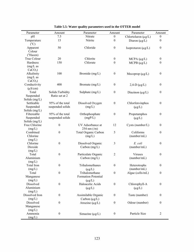
123
Table 5.5: Water quality parameters used in the OTTER model
Parameter Amount Parameter Amount Parameter Amount pH 7.5 Nitrate 0 Chlortoluron (µg/L) 0
Temperature (oC)
15 Nitrite 0 Diuron (µg/L) 0
Apparent Colour
(oHazen)
50 Chloride 0 Isoproturon (µg/L) 0
True Colour 20 Chlorite 0 MCPA (µg/L) 0 Hardness (mg/L as CaCO3)
150 Chlorate 0 MCPB (µg/L) 0
Alkalinity (mg/L as CaCO3)
100 Bromide (mg/L) 0 Mecoprop (µg/L) 0
Conductivity (µS/cm)
400 Bromate (mg/L) 0 2,4-D (µg/L) 0
Total Suspended
Solids (mg/L)
Solids:Turbidity Ratio set at 2
Sulphate (mg/L) 0 Diazinon (µg/L) 0
Settleable Suspended
Solids (mg/L)
95% of the total suspended solids
Dissolved Oxygen (mg/L)
0 Chlorfenvinphos (µg/L)
0
Filtereable Suspended
Solids (mg/L)
95% of the total suspended solids
Orthophosphate (mgP/L)
0 Propetamphos (µg/L)
0
Free Chlorine (mg/L)
0 UV Adsorbance at 254 nm (/m)
12 Cysts (number/L) 0
Combined Chlorine (mg/L)
0 Total Organic Carbon (mg/L)
5 Coliforms (number/mL)
0
Chlorine Dioxide (mg/L)
0 Dissolved Organic Carbon (mg/L)
3 E. coli (number/mL)
0
Total Aluminium
(mg/L)
0 Particulate Organic Carbon (mg/L)
2 Viruses (number/mL)
0
Total Iron (mg/L)
0 Trihalomethanes (µg/L)
0 Heterotrophs (number/mL)
0
Total Manganese
(mg/L)
0 Trihalomethane Formation Potential
(µg/L)
0 Algae (cells/mL) 0
Dissolved Aluminium
(mg/L)
0 Haloacetic Acids (µg/L)
0 Chlorophyll-A (µg/L)
0
Dissolved Iron (mg/L)
0 Assimilable Organic Carbon (µg/L)
0 Taste (number) 0
Dissolved Manganese
(mg/L)
0 Atrazine (µg/L) 0 Odour (number) 0
Ammonia (mg/L)
0 Simazine (µg/L) 0 Particle Size 2

124
5.2.5 Description of Calibrated OTTER Model
Visually, the calibrated OTTER model of Filter 1 can be seen in Figure 5.4. Raw water is passed
through a flow control valve which modifies the flow into the filter. From the filter the treated
water is collected in the process marked “final.” The “wash water” is used for backwashing and
the “waste water” shows the solids accumulation after backwash.
Figure 5.4: OTTER model of Brantford Filter 1
Figure 5.5, Figure 5.6, and Figure 5.7 show the set-up for Filter 1 including all the entered
calibration data. These parameters were constant throughout all the simulations. The model
value, number of CSTR stages, was kept to one (1) for all simulations as discussed in Appendix
C.
Filter Flow Control Valve

125
Figure 5.5: Static data for calibrated Brantford WTP OTTER model
Figure 5.6: Operating data for calibrated Brantford WTP OTTER model

126
Figure 5.7: Calibration data for calibrated Brantford WTP OTTER model
5.2.6 Simulation Convergence Study
Similar to the CFA analysis, a simulation study was performed to see where the simulation
converged. To perform this study, a series of simulations was performed with varying number of
shots. New data sets were developed for each simulation and run through the calibrated OTTER
model. Figure 5.8 and Figure 5.9 show the results from the simulation study. It can be seen that
most percentiles converge well around 13,000 shots; however, as with the simulation study
performed in Chapter 4, this does not hold true with the 99.9th percentile. Future simulations will
use around 13,000 shots but because the 99.9th percentile is not converged, the maximum values
should not be relied on.

127
0.00
0.01
0.01
0.02
0.02
0.03
0.03
0.04
0 2000 4000 6000 8000 10000 12000 14000 16000
Number of Shots
Turb
idity
(NTU
)
10 Percentile50 Percentile80 Percentile90 Percentile
Figure 5.8: Convergence of the calibrated OTTER model simulation: 90 percentile and below
0.00
0.20
0.40
0.60
0.80
1.00
1.20
0 2000 4000 6000 8000 10000 12000 14000 16000
Number of Shots
Turb
idity
(NTU
)
95 Percentile99 Percentile99.9 Percentile
Figure 5.9: Convergence of the calibrated OTTER model simulation: 95 percentile and above
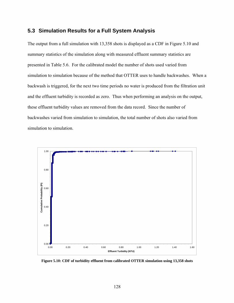
128
5.3 Simulation Results for a Full System Analysis
The output from a full simulation with 13,358 shots is displayed as a CDF in Figure 5.10 and
summary statistics of the simulation along with measured effluent summary statistics are
presented in Table 5.6. For the calibrated model the number of shots used varied from
simulation to simulation because of the method that OTTER uses to handle backwashes. When a
backwash is triggered, for the next two time periods no water is produced from the filtration unit
and the effluent turbidity is recorded as zero. Thus when performing an analysis on the output,
these effluent turbidity values are removed from the data record. Since the number of
backwashes varied from simulation to simulation, the total number of shots also varied from
simulation to simulation.
0.00
0.20
0.40
0.60
0.80
1.00
0.00 0.20 0.40 0.60 0.80 1.00 1.20 1.40 1.60
Effluent Turbidity (NTU)
Cum
ulat
ive
Prob
abili
ty (P
i)
Figure 5.10: CDF of turbidity effluent from calibrated OTTER simulation using 13,358 shots

129
Table 5.6: Summary of output from calibrated OTTER simulation
Simulated Output from Calibrated OTTER
Model (NTU) *
Measured Filter 1 Effluent (NTU)
Max 1.41 0.25 Min 0.00 0.01
Standard Deviation 0.04
0.04
Average 0.02 0.04 95 Percentile 0.03 0.11 99 Percentile 0.07 0.15
* Simulation performed using 13,358 shots
The summary values from Table 5.6 show a discrepancy between what is currently experienced
by the filter and what could possibly occur according to the modelling and probabilistic risk
analysis process. Although the minimums and standard deviations are similar, from a risk
perspective, the results indicate that the measured water quality, at the 95th and 99th percentile
level, produces higher effluent turbidity water than what the model indicates. In other words, the
model predicts a lower actual probability of producing non-compliant water than what is
currently experienced at the water treatment plant.
This lowered probability of producing non-compliant water is illustrated by the divergence in
effluent turbidity values between the simulated data and the measured data with increasing
percentile levels, as shown visually in Figure 5.11. Figure 5.11 shows that as the percentile
levels increase the measured effluent values increase more rapidly than the simulated values.
Chapter 6 provides a detailed discussion on the possible reasons for this difference, primarily
focusing on the ideal versus non-ideal performance of the fitler.

130
0.00
0.20
0.40
0.60
0.80
1.00
0.00 0.20 0.40 0.60 0.80 1.00 1.20 1.40 1.60
Effluent Turbidity (NTU)
Cum
ulat
ive
Prob
abili
ty (P
i)
Measured Effluent
Calibrated Modelwith Random FilterFlow Rate
Figure 5.11: Comparison between measured turbidity effluent and turbidity effluent simulated with a
calibrated model and random filter flow rate
5.3.1 Risk Evaluation
The output from the simulation can be used to evaluate the probability of producing effluent
turbidity greater than a reference level for the filter. Table 5.7 compares the probability of
producing water greater than a reference value between the simulated output and the measured
data for different effluent turbidity targets.
Table 5.7: Risk evaluation for target levels through the calibrated OTTER model
Simulated OTTER model
Effluent (%) Measured Filter 1 Effluent
(%) Probability Effluent Turbidity > 0.05 NTU 1.3 35.8 Probability Effluent Turbidity > 0.10 NTU 0.67 6.9 Probability Effluent Turbidity > 0.30 NTU 0.64 0.0
* Simulation performed with 13,356 shots

131
The output indicates that the filter is operating at a low probability of producing non-compliant
water but this could be misleading especially when comparing the simulated level with the
measured level calculated for the probability of effluent turbidity greater than 0.05 NTU. The
calculated value, 1.3%, differs considerably from that currently experienced by Filter 1, 35.8%.
One possible condition that was evaluated to see if it affected the output was inputting the filter
flow rate as a time-series.
5.3.2 Effect of Time Series Filter Flow Rate
One concern throughout the above analysis involved the filter flow rate that was inputted to the
simulation. This flow rate was assumed to be completely random; however, this assumption is
incorrect. Figure 5.12 shows the flow experienced by Filter 1 over January 2004 while Figure
5.13 shows a simulated flow for approximately one month. Figure 5.12 shows that while the
filter flow rate is slightly random, there is a pattern to the flow which is not visible in Figure
5.13.

132
0
2
4
6
8
10
12
01-Jan 06-Jan 11-Jan 16-Jan 21-Jan 26-Jan 31-Jan
Date
Filte
r Flo
w R
ate
(MLD
)
Figure 5.12: Measured Filter 1 flow rate for January 2004
0
2
4
6
8
10
12
14
16
30-Dec 04-Jan 09-Jan 14-Jan 19-Jan 24-Jan 29-Jan 03-Feb
Date
Filte
r Flo
w R
ate
(MLD
)
Figure 5.13: Simulated Filter 1 flow rate for approximately 1 month

133
5.3.2.1 Results from Filter Analysis by Modified Probabilistic Methodology with
Pseudo-Time Series for Flow Demand
The model set-up and input data initialization was performed as explained in Sections 5.2. The
difference for this simulation was that the filter flow rate profile was not simulated using the
lognormal distribution, but the measured filter flow rate data from 2004 was used as input to the
simulation. It should be noted that by using the 2004 filter flow rate profile the simulation was
no longer completely random and some bias could be input to the simulation. The results from
the simulation can be seen in Figure 5.14 and in Table 5.8.
0.00
0.20
0.40
0.60
0.80
1.00
0.00 0.20 0.40 0.60 0.80 1.00 1.20 1.40 1.60
Effluent Turbidity (NTU)
Cum
ulat
ive
Prob
abili
ty (P
i)
Figure 5.14: CDF of turbidity effluent from calibrated OTTER simulation with time-series filter flow rate
profile

134
Table 5.8: Summary of output from calibrated OTTER simulation with time series filter flow rate profile
Simulated Effluent Turbidity (NTU)* Max 1.45 Min 0.00
Standard Deviation 0.07 Average 0.03
95 0.04 99 0.39
*Simulation Run for 2004 Filter Flow Rate Profile
5.3.2.2 Risk Evaluation
The probability of Filter 1 exceeding target levels can then be calculated. Table 5.9 shows the
calculated and measured levels for Filter 1. The levels that were calculated using a time-series
for the filter flow rate have increased from the completely random filter flow rate shown in Table
5.7; however, there is still some discrepancy between the simulated levels and the measured
Filter 1 levels.
Table 5.9: Risk evaluation for target levels through the calibrated OTTER model using a time series for filter flow rate
Simulated OTTER
Effluent (%)
Measured Filter 1 Effluent (%)
Probability Effluent Turbidity > 0.05 NTU 3.1 35.8 Probability Effluent Turbidity > 0.10 NTU 2.1 6.9 Probability Effluent Turbidity > 0.30 NTU 1.2 0.0
* Simulation performed with one year of actual water demand (34,296 shots)
5.3.3 Comparison between Calibrated OTTER model with random flow demand
and calibrated OTTER model with time-flow series
The differences between using a time series for the filter flow rate and not using a time series can
be seen in Table 5.10 and Table 5.11. The numerical values of the probability of producing non-

135
compliant water, as seen in Table 5.10, change by approximately 1-2 percentage points for the
three different levels. However, it is in the numerical effluent turbidity output that differences
can be seen. Table 5.11 shows that the time-series filter flow rate curve allows for slightly
higher turbidity effluent on average and at the 95 percentile level and substantially higher
effluent turbidity at the 99 percentile level. This occurs because the time-series causes a greater
percentage of the output values to be larger, as can be seen in Figure 5.15.
Table 5.10: Comparison between probabilistic risk evaluation using a calibrated OTTER model with and without a time series for water flow
Calibrated OTTER Model* Calibrated OTTER Model Time
Series **
Median
(%)
Upper Bound
(%)
Lower Bound
(%) Range
(%) Median
(%)
Upper Bound
(%)
Lower Bound
(%) Range
(%) Probability > 0.05 NTU 1.3 1.5 1.1 0.4 3.1 3.3 2.9 0.4 Probability > 0.10 NTU 0.7 0.8 0.5 0.3 2.1 2.3 2.0 0.3 Probability > 0.30 NTU 0.6 0.8 0.5 0.3 1.2 1.4 1.1 0.2
* Simulation performed using 13,358 shots ** Simulation performed with 2004 year of actual filter flow rate (34,296 shots)
Table 5.11: Comparison of probabilistic risk analysis output using a calibrated OTTER model with and without a time series for water flow
Calibrated OTTER Model*
Calibrated OTTER
Model Time Series **
Max (NTU) 1.41 1.45
Min (NTU) 0.00 0.00 Standard Deviation
(NTU) 0.04 0.07
Average (NTU) 0.02 0.03 95 Percentile (NTU) 0.03 0.04 99 Percentile (NTU) 0.07 0.39
Average Filter Run Time (hrs) 80 100
* Simulation performed using 13,358 shots ** Simulation performed with 2004 year of actual filter flow rate (34,296 shots)

136
0.90
0.95
1.00
0.00 0.20 0.40 0.60 0.80 1.00 1.20 1.40 1.60
Effluent Turbidity (NTU)
Cum
ulat
ive
Prob
abili
ty (P
i)
CalibratedModel withRandom FilterFlow Rate
CalibratedModel withTime-SeriesFilter Flow Rate
Figure 5.15: Comparison of the CDF output from the probabilistic risk assessment for the calibrated OTTER
models with and without using a time series: Focusing on the top 10% of the CDF
One possible reason for the difference between the simulations with and without a time-series
filter flow rate can be deduced from the average filter run times. The calibrated model with
random filter flow rate has an average of 80 hours per filter run, while the calibrated model using
the time series has an average of 100 hours per filter run. The longer filter runs for the time-
series flow rate allowed for higher effluent turbidity output and thus a higher probability of
producing non-compliant water.
This analysis shows how the mechanism used to model the filter flow rate can affect the output
from the analysis. However, because the 2004 data record is not random the rest of the thesis
will use the results from the simulations performed with the completely random filter flow rate.

137
Any future study should evaluate in more detail the mechanism of incorporating filter flow rate
into the analysis.
5.4 Predictive Modelling and Risk Analysis
The use of a calibrated computer model allows for a more comprehensive analysis of the
treatment process, which is not possible with other risk analysis methodologies such as the CFA.
One area of further analysis is through using the computer model and the risk analysis
methodology to analyze predictive scenarios. Predictive scenarios would involve changing the
input or calibrated parameters within the computer model and determining how the final output
would be affected. It is possible to choose any number of different parameters to evaluate
including any physical, operational or calibration parameters. For the analysis three factors were
changed: influent water turbidity, filter flow rate, and filter depth. These three factors were
chosen because Letterman (1987) mentions them during his evaluation of factors that affect
filtered water quality and headloss development and because time constraints limited the analysis
to only three factors.
5.4.1 Predictive Study Set-Up
The predictive study was set up in a manner similar to a 23 factorial study. The three parameters
were combined together to form eight different simulations which cover the range of input values
for these parameters. Table 5.12 shows the simulation set-up. The simulation numbers in Table
5.12 were chosen arbitrarily to identify the different filter runs. They start at number 6 because
numbers 1 through 5 were used during some preliminary analysis that is not reported on in this
thesis.

138
Table 5.12: Predictive study using computer modelling set-up
Simulation # Filter Depth Influent Turbidity
Filter Flow Rate
11 Low Low Low
13 Low Low High
12 Low High Low
10 Low High High
7 High Low Low
9 High Low High
8 High High Low
6 High High High
Saatci and Oulman (1980) caution against extrapolating data beyond the depths and filter flow
rates used to generate the calibrated parameters. Thus low and high values were chosen to be
20% above and below the original values respectively. Because the influent turbidity and filter
flow rate are distributions and not single values, it was decided to increase and decrease the
mean of the measured data and not modify the standard deviation. Thus, increasing or
decreasing the mean by 20% would represent a series of new measurements where the average
would be 20% higher or lower than the original average but with the same standard deviation.
Since the chosen distribution was lognormal, this required that both the mean and standard
deviation of the lognormal distribution be modified so that only the mean of the data that is not
logged would change. Figure 5.16 shows this visually for simulated data for influent turbidity.
The same procedure was followed for filter flow rate.

139
0
500
1000
1500
2000
2500
0.00
0.10
0.20
0.30
0.40
0.50
0.60
0.70
0.80
0.90
1.00
1.10
1.20
1.30
1.40
1.50
1.60
1.70
1.80
Bin Range (NTU)
Freq
uenc
y (#
)
Original LognormalInfluent TurbidityDistribution
20% HigherLognormal InfluentTurbidityDistribution
20% LowerLognormal InfluentTurbidityDistribution
Figure 5.16: High and low distributions for influent turbidity for the predictive study
The input data for the eight different simulations can be seen in Table 5.13. For influent
turbidity and filter flow rate, the values in Table 5.13 show the mean of the simulated data set.
Table 5.13: Input data for the different simulations for the predictive study
Simulation # Filter Depth
(m)
Influent Turbidity (NTU)
Filter Flow Rate (MLD)
11 0.7312 0.252 4.94
13 0.7312 0.252 7.42
12 0.7312 0.378 4.94
10 0.7312 0.378 7.42
7 1.0968 0.252 4.94
9 1.0968 0.252 7.42
8 1.0968 0.378 4.94
6 1.0968 0.378 7.42

140
5.4.2 Simulation Output
The output from the simulations was evaluated using Yates method. This analysis determined
the effects and sums of squares for each parameter of interest. Appendix E shows the full
calculations for all the simulations, while Table 5.14 and Table 5.15 provide an overview of the
findings. Table 5.14 shows the output from the analysis while Table 5.15 shows the calculated
effects and interactions of each parameter in the analysis.
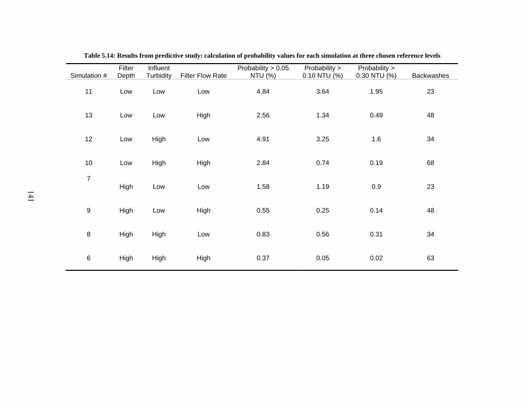
Table 5.14: Results from predictive study: calculation of probability values for each simulation at three chosen reference levels
Simulation # Filter Depth
Influent Turbidity Filter Flow Rate
Probability > 0.05 NTU (%)
Probability > 0.10 NTU (%)
Probability > 0.30 NTU (%) Backwashes
11 Low Low Low 4.84 3.64 1.95 23
13 Low Low High 2.56 1.34 0.49 48
12 Low High Low 4.91 3.25 1.6 34
10 Low High High 2.84 0.74 0.19 68
7 High Low Low 1.58 1.19 0.9 23
9 High Low High 0.55 0.25 0.14 48
8 High High Low 0.83 0.56 0.31 34
6 High High High 0.37 0.05 0.02 63
141
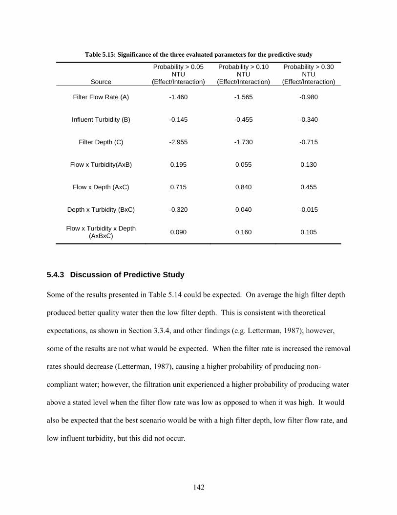
142
Table 5.15: Significance of the three evaluated parameters for the predictive study
Source
Probability > 0.05 NTU
(Effect/Interaction)
Probability > 0.10 NTU
(Effect/Interaction)
Probability > 0.30 NTU
(Effect/Interaction)
Filter Flow Rate (A) -1.460 -1.565 -0.980
Influent Turbidity (B) -0.145 -0.455 -0.340
Filter Depth (C) -2.955 -1.730 -0.715
Flow x Turbidity(AxB) 0.195 0.055 0.130
Flow x Depth (AxC) 0.715 0.840 0.455
Depth x Turbidity (BxC) -0.320 0.040 -0.015
Flow x Turbidity x Depth (AxBxC) 0.090 0.160 0.105
5.4.3 Discussion of Predictive Study
Some of the results presented in Table 5.14 could be expected. On average the high filter depth
produced better quality water then the low filter depth. This is consistent with theoretical
expectations, as shown in Section 3.3.4, and other findings (e.g. Letterman, 1987); however,
some of the results are not what would be expected. When the filter rate is increased the removal
rates should decrease (Letterman, 1987), causing a higher probability of producing non-
compliant water; however, the filtration unit experienced a higher probability of producing water
above a stated level when the filter flow rate was low as opposed to when it was high. It would
also be expected that the best scenario would be with a high filter depth, low filter flow rate, and
low influent turbidity, but this did not occur.

143
The seemingly improbable observation that a low filter flow rate produced a worse situation than
a high flow rate can be explained through the understanding of backwashes. Initially, it is
important to remember that an increase in filter flow rate increases the rate of headloss
development (Letterman, 1987) which is also consistent with the Carman Kozeny equation as
shown in Section 3.3.3. This effect of filter flow rate on headloss development can be seen in
Figure 5.17, as the low filter flow rate scenario in Simulation 11 has a lower rate of headloss
build up than the high filter flow rate scenario (Simulation 13).
0.00
0.50
1.00
1.50
2.00
2.50
0 50 100 150 200 250 300 350
Run Time (hrs)
Hea
dlos
s (m
)
Simulation 11: Low Filter Flow RateSimulation 13: High Filter Flow Rate
Figure 5.17: Headloss build up in the filtration unit over time for Simulations 11 and 13
Since the filtration unit in question operates under a headloss trigger only, the model study shows
that the filter flow rate is a major contributor to the number of backwashes. For example,
Simulations 11 and 13 have the exact same characteristics except for the filter flow rate and the

144
high filter flow rate causes a greater number of backwashes per volume of water filtered. This
can be seen in Figure 5.18.
0
5
10
15
20
25
30
35
0 100000 200000 300000 400000 500000 600000 700000
Filtered Water Volume (m3)
Num
ber o
f Bac
kwas
hes
Simulation 11: Low Filter Flow RateSimulation 13: High Filter Flow Rate
Figure 5.18: Backwashes over time for Simulations 11 and 13
A calculation for Simulation 11 and Simulation 13 showed that for equivalent filtered water
volumes the two simulations removed the same amount of total solids. This was determined by
looking at the average turbidity removed per volume of water filtered for a series of filter runs
for both simulations such that the total amount of water filtered was similar. The unit of
comparison is the ratio of the average amount of solids removed per filtered water volume,
averaged for the total number of filter runs for Simulation 11 and for the number of filter runs for
Simulation 13 which corresponds to approximately the same amount of total water filtered for
Simulation 11. This analysis is shown in Table 5.16. Since the calculated t-statistic is below the

145
critical t-statistic, the two simulations are shown to remove approximately the same amount of
solids per filtered water volume over an equal amount of filtered water volume. The calculations
performed in Table 5.16 were performed for the condition where the variances of the different
simulations cannot be assumed to be equal.
Table 5.16: T-test to compare the turbidity removal between simulation 11 and simulation 13
Simulation 11 Simulation 13 N (number of filter runs) 22 29 Average ratio of kg of solids removed per volume of water filtered (kg/m3)
4.50E-04 4.59E-04
Standard Deviation of the ratio of kg of solids removed per volume of water filtered
1.75E-05 4.32E-05
Observed T statistic 1.030 Degrees of freedom 39 Critical T statistic for t39,0.025 2.021
Although the amount of solids per filtered water volume is similar, the higher filter flow rate in
Simulation 13 caused a greater number of backwashes and lowered effluent turbidity values.
Figure 5.19, although hard to evaluate, shows this decrease in turbidity by the larger proportion
of higher effluent turbidity values from Simulation 11 as opposed to Simulation 13.
With a fewer number of backwashes per unit volume, the lower flow rate allows the filter to
experience more time with a higher solids loading in the bed. As described in Section 3.3.4, the
total attachment of particles to a filter bed is a function of the attachment and detachment. With
a longer period of time in the filter bed, there is the possibility that a greater number of particles
could detach, contributing to the higher effluent water quality. With the high filter flow rate, this

146
condition is not experienced. Therefore, for the current filter operation, the situation of concern
is one of low filter flow rate, which allows higher effluent turbidity.
0.00
0.20
0.40
0.60
0.80
1.00
1.20
1.40
1.60
1.80
0 500 1000 1500 2000 2500 3000 3500
Run Time (hrs)
Efflu
ent T
urbi
dity
(NTU
)
Simulation 11: Low Filter Flow RateSimulation 13: High Filter Flow Rate
Figure 5.19: Turbidity effluent from the filtration unit over time for Simulations 11 and 13
One difficulty in using the factorial study methodology with simulated data occurred during the
evaluation of the output. Although each simulation was performed for the same number of input
values, each time a backwash occurred the filter did not produce water for that time period. This
effectively lowered the total number of shots for the effluent turbidity. Since each simulation
had a different number of backwashes, each simulation also had a different number of shots.
The evaluation of a factorial study uses a mean square error, a measurement related to the
standard deviation, to determine whether a parameter is significant or not. Since the standard

147
deviation is based on the number of shots and the mean of the simulation, see Section 4.5, each
simulation will have a different standard deviation. Over the course of the eight different
simulations, the total number of shots varied by 90, but the standard deviation between one
simulation and another varied by a factor of 100. Thus a standard deviation or mean square error
was not determined directly from the simulations.
To calculate the significance of the different effects and interactions, a normal probability plot
was used. The normal probability plot evaluates the different calculated effects and interactions
with the expectation that the differences between them are from to random variation (e.g.
Montgomery, 2001), consequently the change of one or more variable would not have an effect
on the output. If this was true then all the effects and interactions would fall on a straight line on
a normal probability plot while any factors that do not fall on a straight line can then be
determined to be significant (Montgomery, 2001). The normal probability plot can also be used
to gain an estimate of the error associated with the analysis by using the insignificant effects as
an estimate of the error (Montgomery, 2001), allowing for the use of an F-test to determine the
significant effects. Both of these methods were used in this analysis.
Table 5.17, Table 5.18, and Table 5.19 provide the F-tests at the 5% significance level for the
three different conditions. The error was estimated in all situations from the three most
insignificant effects: BC, ABC, AB. These tables show that the filter flow rate (A) and filter
depth (C) are both significant factors while the filter flow rate by filter depth interaction (AC) is
significant for one of the conditions. If the significance level was lowered, the filter flow rate by
filter depth interaction would be significant for all three conditions.

148
Table 5.17: F-test for the probability of effluent turbidity greater than 0.05 NTU
Source Effect SS DF MS F Significant Filter Flow Rate
(A) -1.460 4.263 1 4.263 14.352 Yes Influent Turbidity
(B) -0.145 0.042 1 0.042 0.142 No
Filter Depth (C) -2.955 17.464 1 17.464 58.792 Yes
Flow x Turbidity(AxB) 0.195 0.076 1 0.076 0.256 No
Flow x Depth (AxC)
0.715 1.022 1 1.022 3.442 No Depth x
Turbidity (BxC) -0.320 0.205 1 0.205 0.689 No
Flow x Turbidity x Depth (AxBxC)
0.090 0.016 1 0.016 0.055 No
Error 3 0.297 Note: fcrit = f1,3,0.05 = 10.13
Table 5.18: F-test for the probability of effluent turbidity greater than 0.10 NTU
Source Effect SS DF MS F Significant Filter Flow Rate
(A) -1.565 4.898 1 4.898 81.033 Yes Influent Turbidity
(B) -0.455 0.414 1 0.414 6.849 No Filter Depth (C) -1.730 5.986 1 5.986 99.021 Yes
Flow x Turbidity(AxB) 0.055 0.006 1 0.006 0.100 No Flow x Depth
(AxC) 0.840 1.411 1 1.411 23.345 Yes
Depth x Turbidity (BxC)
0.040 0.003 1 0.003 0.053 No
Flow x Turbidity x Depth (AxBxC)
0.160 0.051 1 0.051 0.847 No
Error 3 0.060 Note: fcrit = f1,3,0.05 = 10.13
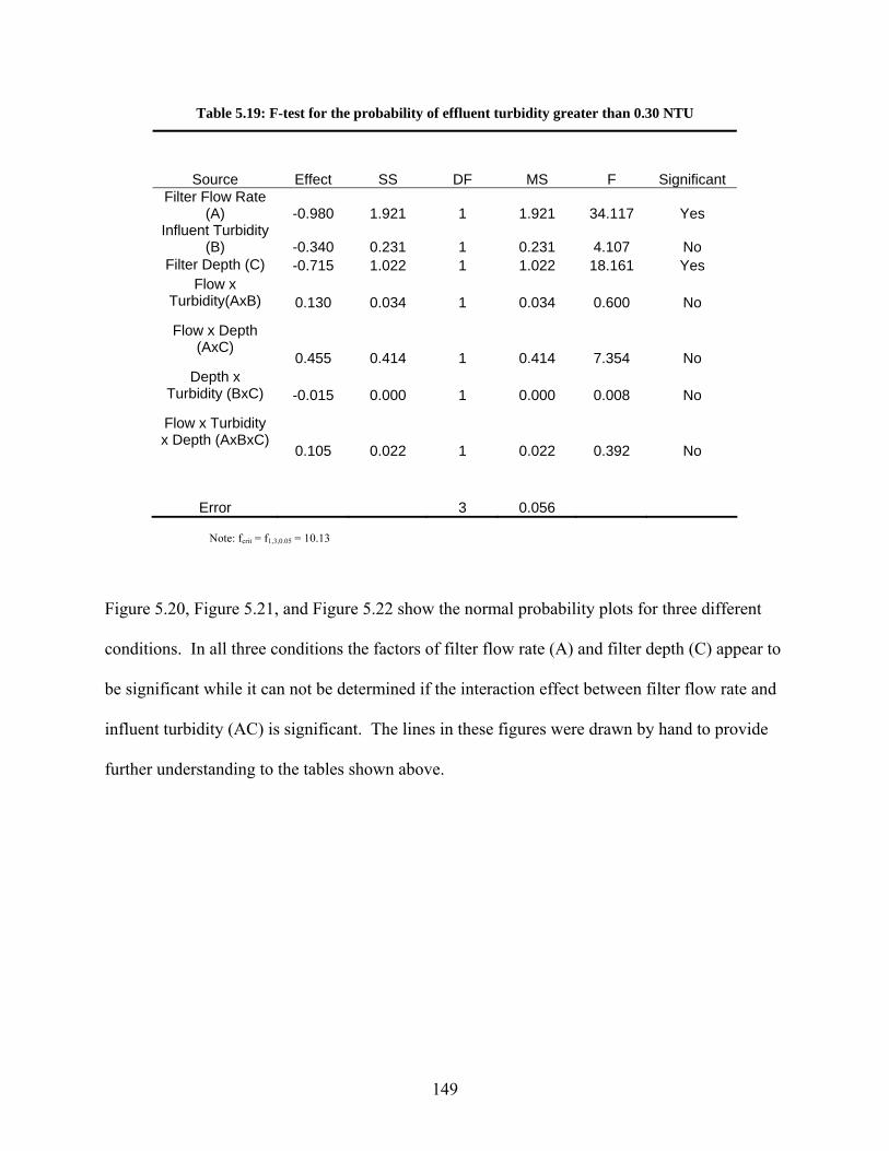
149
Table 5.19: F-test for the probability of effluent turbidity greater than 0.30 NTU
Source Effect SS DF MS F Significant Filter Flow Rate
(A) -0.980 1.921 1 1.921 34.117 Yes Influent Turbidity
(B) -0.340 0.231 1 0.231 4.107 No Filter Depth (C) -0.715 1.022 1 1.022 18.161 Yes
Flow x Turbidity(AxB) 0.130 0.034 1 0.034 0.600 No
Flow x Depth (AxC)
0.455 0.414 1 0.414 7.354 No Depth x
Turbidity (BxC) -0.015 0.000 1 0.000 0.008 No
Flow x Turbidity x Depth (AxBxC)
0.105 0.022 1 0.022 0.392 No
Error 3 0.056 Note: fcrit = f1,3,0.05 = 10.13
Figure 5.20, Figure 5.21, and Figure 5.22 show the normal probability plots for three different
conditions. In all three conditions the factors of filter flow rate (A) and filter depth (C) appear to
be significant while it can not be determined if the interaction effect between filter flow rate and
influent turbidity (AC) is significant. The lines in these figures were drawn by hand to provide
further understanding to the tables shown above.

150
-1.50
-1.00
-0.50
0.00
0.50
1.00
1.50
-3.50 -3.00 -2.50 -2.00 -1.50 -1.00 -0.50 0.00 0.50 1.00
Effects
Expe
cted
Nor
mal
Val
ue
C
A
BC
B
ABC
AB
AC
Figure 5.20: Normal probability plot for the probability of effluent turbidity greater than 0.05 NTU (A: filter
flow rate, B: filter depth, C: influent turbidity)
-1.50
-1.00
-0.50
0.00
0.50
1.00
1.50
-2.00 -1.50 -1.00 -0.50 0.00 0.50 1.00
Effects
Expe
cted
Nor
mal
Val
ue
C
A
B
BC
AB
ABC
AC
Figure 5.21: Normal probability plot for the probability of effluent turbidity greater than 0.10 NTU (A: filter
flow rate, B: filter depth, C: influent turbidity)
Filter Depth
Filter Flow Rate
Filter Depth
Filter Flow Rate
Depth x Filter Flow Rate

151
-1.50
-1.00
-0.50
0.00
0.50
1.00
1.50
-1.20 -1.00 -0.80 -0.60 -0.40 -0.20 0.00 0.20 0.40 0.60
Effects
Expe
cted
Nor
mal
Val
ue
A
C
B
BC
ABC
AB
AC
Figure 5.22: Normal probability plot for the probability of effluent turbidity greater than 0.30 NTU (A: filter
flow rate, B: filter depth, C: influent turbidity)
5.5 Risk Analysis Implications for the Brantford Water Treatment
Plant
If this analysis was performed for a regulatory agency with a requirement that the turbidity must
be below 0.30 NTU 95% of the time, then the risk analysis methodology using a random filter
flow rate in conjunction with the OTTER model and the measured data would satisfy this
criteria. However, if the regulatory requirement was 0.10 NTU 95% of the time, then the
probabilistic analysis with the OTTER model would satisfy this criterion but the measured data
would not. This is described in Section 5.3.1. The difference between the regulatory acceptance
or rejection depending on whether measured or simulated data is used illustrates the importance
that should be placed on determining how the calculations for compliance should be performed.
Filter Depth
Filter Flow Rate

152
The results from the risk analysis methodology using a random filter flow rate in conjunction
with the OTTER model can be incorporated with idea of conditional reliability in a similar way
that the results from the CFA were. However, to analyze the results from the calibrated OTTER
model, the methodology used for the CFA was expanded upon to evaluate three different
conditional situations. The first looked at the filter flow rate, the second at the influent turbidity,
and the third analyzed a combination of the filter flow rate and the influent turbidity Table 5.20
shows the output from this analysis.
Table 5.20: Conditional reliability analysis of calibrated OTTER model
Condition Probability Effluent Turbidity > 0.05 NTU
Filter Flow Rate Filter Flow Rate Less than (0.679); υ−σ in the lognormal distribution 0.00
Filter Flow Rate Between (0.679 and 0.880); υ−σ and υ+σ in the lognormal distribution 0.01
Filter Flow Rate Greater than (.880); υ+σ in the lognormal distribution 0.04
Influent Turbidity Influent Turbidity Less than (-0.732); υ−σ in the lognormal distribution 0.01
Influent Turbidity Between (-0.732 and -0.353); υ−σ and υ+σ in the lognormal distribution 0.01
Influent Turbidity Greater than (-.353); υ+σ in the lognormal distribution 0.02
Combination Filter Flow Rate Less than υ−σ and Influent Turbidity Less than υ−σ 0.00
Filter Flow Rate Less than υ−σ and Influent Turbidity Between υ−σ and υ+σ 0.00
Filter Flow Rate Less than υ−σ and Influent Turbidity Greater than υ+σ 0.01
Filter Flow Rate Between υ−σ and υ+σ and Influent Turbidity Less than υ−σ 0.01
Filter Flow Rate Between υ−σ and υ+σ and Influent Turbidity Between υ−σ and υ+σ 0.01
Filter Flow Rate Between υ−σ and υ+σ and Influent Turbidity Greater than υ+σ 0.01
Filter Flow Rate Greater than υ+σ and Influent Turbidity Less than υ−σ 0.04
Filter Flow Rate Greater than υ+σ and Influent Turbidity Between υ−σ and υ+σ 0.04
Filter Flow Rate Greater than υ+σ and Influent Turbidity Greater than υ+σ 0.06

153
The output from the calibrated model, as shown in Table 5.20, shows the probability of
producing effluent turbidity greater than 0.05 NTU for a series of conditions. Although 0.05
NTU is not important from a regulatory prospective, it was used for this analysis as it might be
important from an operational perspective. Table 5.20 shows that the probability of producing
effluent turbidity greater than 0.05 NTU increases with influent turbidity as would be expected.
However, while the probability increases by a factor of two for the influent water quality
between the low influent and the high influent, the filter flow rate shows an increase by a factor
of four. This indicates that filter flow rate has a greater effect on the effluent water quality than
the influent turbidity, for the data analyzed. This observation is illustrated more succinctly when
the filter flow rate is greater than the mean plus one standard deviation. Under these conditions,
the probability of producing water quality greater than 0.05 NTU remains above 4% regardless
of the influent turbidity.
The predictive study, discussed in Section 5.4.3, corroborates the findings of the conditional
reliability study by showing the significance of the filter flow rate and furthers this understanding
by showing the importance of the filter depth for this filtration unit. However, some
discrepancies are noticed. It should be mentioned that the conditional reliability methodology
uses the output from the risk analysis with the OTTER model directly without any extrapolation
of the input data. However, the predictive study uses a series of inputs that result in higher and
lower influent turbidity and filter flow rates than are seen through the 2004 data record. This
could account for some of the discrepancies.

154
Nevertheless, the predictive study indicates that the a decrease in the filter flow rate increases the
probability of producing water above a stated level while an increase in filter flow rate decreases
the probability. The conditional reliability study shows a relationship where an increase in filter
flow rate results in an increase in the probability of producing water above a stated level. So
while the predictive study indicates that a low flow condition is of concern, the conditional
reliability study indicates that a high flow condition is of concern.
In an attempt to reconcile this difference, two of the predictive simulations were run a second
time with an added 0.30 NTU backwash turbidity trigger. Table 5.21 shows that the backwash
turbidity trigger lowered the probability of producing effluent turbidity greater than a standard.
In the case of Simulation 11, a backwash turbidity trigger decreased the probability of producing
effluent turbidity greater than 0.10 NTU from 3.46% to 0.46%.
Evaluating Table 5.21 for the relationship between Simulations 10 and 11 without backwash
turbidity triggers, it can be seen that Simulation 11, a low flow rate simulation, exhibits more
risk than the high flow rate Simulation 10. However, after including the backwash turbidity
triggers, the high flow rate Simulation 10, contains more risk than the low flow rate Simulation
11. This is what was originally expected and what was seen in the conditional reliability study; a
higher flow rate increases the probability of producing effluent turbidity greater than some value.
Thus the discrepancy between the conditional reliability study and the predictive study is
partially resolved by adding a turbidity trigger.

155
Theoretically, this study illustrates that a measure of caution should always be used before
utilizing an analysis method. Practically, this study illustrates that one method to decrease the
risk associated with producing effluent turbidity greater than a reference is to ensure no low flow
conditions occur, while another method is to add a backwash turbidity trigger to the filtration
unit. Adding a time trigger for backwashing would also lower the probability of producing
effluent turbidity greater than some level however this condition was not evaluated in this thesis.
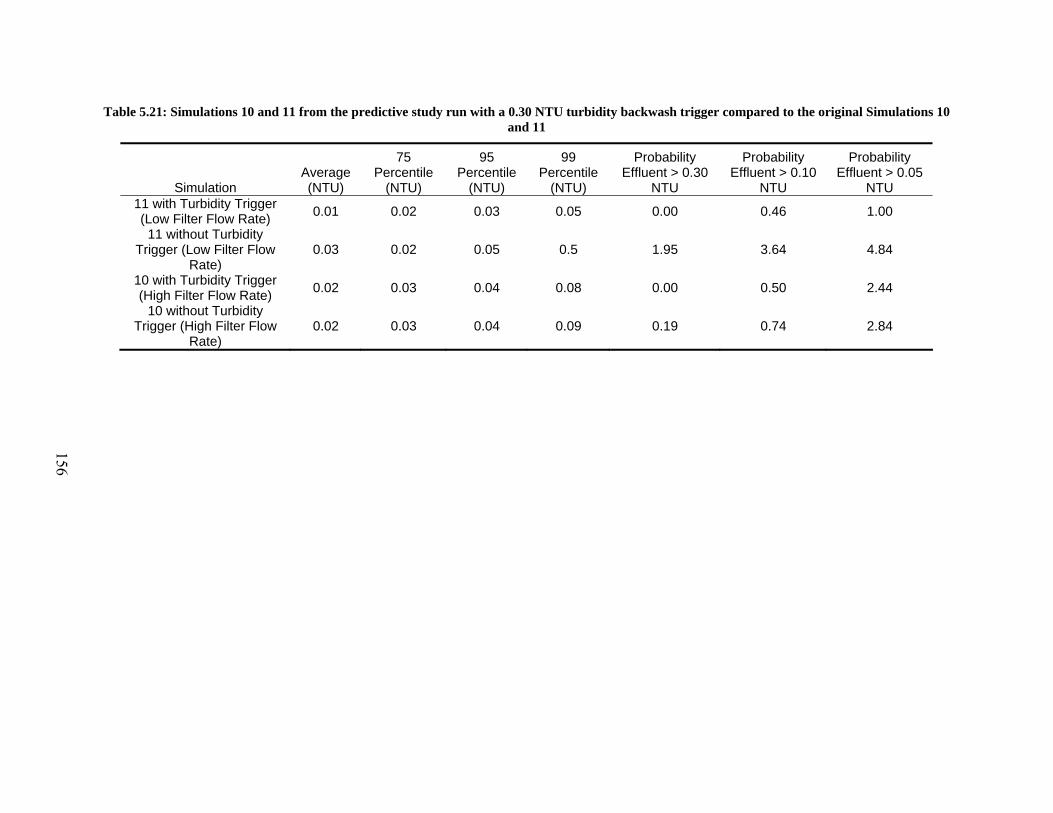
Table 5.21: Simulations 10 and 11 from the predictive study run with a 0.30 NTU turbidity backwash trigger compared to the original Simulations 10 and 11
Simulation Average (NTU)
75 Percentile
(NTU)
95 Percentile
(NTU)
99 Percentile
(NTU)
Probability Effluent > 0.30
NTU
Probability Effluent > 0.10
NTU
Probability Effluent > 0.05
NTU 11 with Turbidity Trigger (Low Filter Flow Rate) 0.01 0.02 0.03 0.05 0.00 0.46 1.00
11 without Turbidity Trigger (Low Filter Flow
Rate) 0.03 0.02 0.05 0.5 1.95 3.64 4.84
10 with Turbidity Trigger (High Filter Flow Rate) 0.02 0.03 0.04 0.08 0.00 0.50 2.44
10 without Turbidity Trigger (High Filter Flow
Rate) 0.02 0.03 0.04 0.09 0.19 0.74 2.84
156

157
CHAPTER 6 DISCUSSION OF RISK ANALYSIS METHODOLOGIES
6.1 Numerical Differences
A comparison of the two different risk analysis methodologies and the measured data can be
seen in Table 6.1 and a comparison of the risk evaluation from the different methodologies for
three different levels can be seen in Figure 6.1, Figure 6.2, and Figure 6.3. From looking at
Table 6.1, it is difficult to determine which risk analysis methodology should be used for future
analysis. The output from the CFA generally matches the turbidity effluent that is currently
experienced by Filter 1; however, there are extremely high effluent values that are above
anything seen presently by Filter 1. The output from the probabilistic methodology using the
calibrated OTTER model seems to underestimate the actual turbidity effluent, except for the
maximums values.
A comparison of the risk evaluation methodologies shows that at the 0.05 NTU level (Figure
6.1), the CFA and the measured effluent are reasonably similar but the probabilistic methodology
using the calibrated OTTER model differs considerably. As the level increases to the 0.10 NTU
(Figure 6.2), and the 0.30 NTU range (Figure 6.3), the different methodologies begin to produce
similar results. In evaluating the Figure 6.1, Figure 6.2, and Figure 6.3 it should be noted that the
confidence limits in Figure 6.1, Figure 6.2, and Figure 6.3 remain reasonably similar as they are

158
based on the number of simulations, as discussed in Section 4.5, and that the scale changes from
one figure to another.
Table 6.1: Comparison of risk analysis methodologies using output from the simulations
Consequence Frequency
Assessment*
Calibrated OTTER Model**
Measured Filter 1 Effluent
Max 2.92 1.41 0.25
Min 0.00 0.00 0.01 Standard Deviation 0.06 0.04 0.04
Average 0.05 0.02 0.05 95 Percentile 0.15 0.03 0.11 99 Percentile 0.28 0.07 0.15
* CFA performed for 180,000 shots ** Calibrated OTTER simulation performed for 13,358 shots
0.0 5.0 10.0 15.0 20.0 25.0 30.0 35.0 40.0
Probability Effluent Turbidity > 0.05 NTU (%)
Consequence FrequencyAssessment
Calibrated Model with RandomFilter Flow Rate
Sim
ulat
ion
Met
hodo
logy
Filter 1 Effluent: 35.8%
95 % Confidence Limits: 1.1 - 1.5%
95 % Confidence Limits: 29.7 - 30.1%
Figure 6.1: Comparison of risk evaluation from different analysis methodologies for probability of producing
water greater than 0.05 NTU

159
0.0 2.0 4.0 6.0 8.0 10.0 12.0
Probability Effluent Turbidity > 0.10 NTU (%)
Consequence FrequencyAssessment
Calibrated Model with Random FilterFlow Rate
Sim
ulat
ion
Met
hodo
logy
Filter 1 Effluent: 6.9%
95 % Confidence Limits: 0.53 - 0.81%
95 % Confidence Limits: 10.3 - 10.5%
Figure 6.2: Comparison of risk evaluation from different analysis methodologies for probability of producing
water greater than 0.10 NTU
0.0 0.1 0.2 0.3 0.4 0.5 0.6 0.7 0.8 0.9
Probability Effluent Turbidity > 0.30 NTU (%)
Consequence FrequencyAssessment
Calibrated Model with Random FilterFlow Rate
Sim
ulat
ion
Met
hodo
logy
Filter 1 Effluent: 0.0%
95 % Confidence Limits: 0.50 - 0.77%
95 % Confidence Limits: 0.77 - 0.85%
Figure 6.3: Comparison of risk evaluation from different analysis methodologies for probability of producing
water greater than 0.30 NTU

160
A more comprehensive understanding of the different methodologies can be seen by looking at
Figure 6.4. In this figure, it is evident that until around the 95th percentile the measured effluent
and the CFA are closely related while the probabilistic analysis with the OTTER model seems to
underestimate the measured effluent until around the 99th percentile, above which it greatly
exceeds it. Figure 6.5 shows this difference more explicitly by limiting scale along the x-axis of
Figure 6.4 to 0.5 NTU.
0.90
0.95
1.00
0.00 0.50 1.00 1.50 2.00 2.50 3.00 3.50
Effluent Turbidity (NTU)
Cum
ulat
ive
Prob
abili
ty (P
i)
Measured Effluent
Calibrated Model withRandom Filter FlowRate
CFA Simulation
Figure 6.4: CDF of the output from the different risk analysis methodologies and the measured effluent:
Focusing on the top 10% of the CDF

161
0.00
0.20
0.40
0.60
0.80
1.00
0.00 0.05 0.10 0.15 0.20 0.25 0.30 0.35 0.40 0.45 0.50
Effluent Turbidity (NTU)
Cum
ulat
ive
Prob
abili
ty (P
i)
Measured Effluent
Calibrated Modelwith Random FilterFlow Rate
CFA Simulation
Figure 6.5: CDF of the output from the different risk analysis methodologies and the measured effluent:
Focusing on the top 10% of the CDF and between 0 - 0.5 NTU
The question is which methodology to use and what the different methodologies are measuring.
There are three possible outcomes from this analysis and comparison:
1) Combining modelling and probabilistic simulation produces more reasonable values from
a risk perspective in comparison to other methodologies such as the CFA or in
comparison to past measured data.
2) The discrepancies between the CFA and the combination of probabilistic simulation with
modelling can be accounted for because of the assumptions that were necessary to
perform the analysis.

162
3) The different methodologies are measuring different aspects of risk.
The first possible outcome cannot be stated with certainty before the assumptions of the analysis
are checked and the other two possible outcomes are discounted. Therefore to eliminate the
second possible outcome, the basic assumptions of the OTTER modelling procedure and risk
analysis procedure should be checked. Some of the basic assumptions are that the modified
calibration procedure was reasonable, that a time series filter flow rate curve could be simplified
to be completely random, and that the OTTER filter model sufficiently describes the filtration
process. The assumption that a completely random filter flow rate could be used was tested by
using the 2004 data record and some differences were seen between using the two different
methods of generating filter flow rates. However, the 2004 data record was not completely
random and thus a random filter flow rate curve which incorporates the time-series component
should be used in a future study to see of the output is affected.
The third possible outcome provides an interesting discussion that should require more
investigation. In using a calibrated software model, the risk analysis is performed on a set of
ideal operating conditions. This was an initial goal of the analysis, to determine the probability
of producing water above a specified reference level from a properly operated water treatment
plant. The simulations show that this probability for the filtration unit analyzed is between 1%
and 3% depending whether the reference level is 0.3 NTU of 0.05 NTU. However, the CFA is
based on the past data record exclusively, which will include non-ideal conditions or situations
where operational procedures were modified. For example, the backwashing of a filter manually
163
because the operator perceives it is necessary. The discrepancy between the CFA and the
modelled risk evaluation would then be those conditions that could be classified as non-ideal.
One assumption in making this comparison is that the data record used in the CFA would have
no instances where the output would be affected by a mechanical failure, which would need to be
analyzed using a mechanical risk analysis methodology. There was no way of knowing this for
the gathered data set.
Therefore, the difference in output from the risk methodologies would converge when the
modelled probabilistic methodology found a mechanism to incorporate non-ideal conditions into
the analysis. If, after further analysis, the third possible outcome was deemed to be reasonable,
then a recommendation might be that an analysis mechanism such as the CFA is sufficient for
simplified risk analysis, but that for a more comprehensive understanding of the system a risk
methodology using modelling and probabilistic analysis could be performed with the
understanding that it focuses on the ideal conditions.
6.2 External Differences
One of the major differences between the CFA and using modelling and probabilistic risk
analysis is the wider range of capabilities with the use of computer modelling. Using computer
modelling allowed the effect of external parameters, such as filter flow rate, to be included in the
overall analysis. In this instance it showed that the filter flow rate was a greater contributor to
producing non-compliant water than influent turbidity. Also, using computer modelling allowed
for predictive studies. In this case, it was shown that adding a backwash turbidity trigger to the
filtration unit would greatly reduce the probability of producing non-compliant water for low
filter flow rate scenarios. Furthermore, the predictive studies showed that the filter flow rate and
164
filter depth were the most significant effects on the probability of producing effluent turbidity
greater than a reference level. Influent turbidity, although not significant in this study, could be
important in other situations. The CFA, in its current form, is unable to analyze any of these
things.
6.3 Risk Analysis Implications for the Brantford Water Treatment
Plant
The results from the risk analysis using the two methods showed results that were at times highly
divergent. An example of this is the probability of producing turbidity effluent greater than 0.05
NTU. The consequence frequency assessment calculated a value of approximately 30% while
the probabilistic methodology with model simulation calculated a value of approximately 1%.
The Brantford WTP filtration unit is directed by the Ontario Drinking Water Standards which
have a 5 NTU maximum turbidity at the point of consumption (Ontario Ministry of the
Environment, 2003). However a more comprehensive regulation of turbidity is provided by the
Guidelines for Canadian Drinking Water which, for chemically assisted filtration, direct that
turbidity “shall be less than or equal to 0.3 NTU in at least 95% of the measurements made, or at
least 95% of the time each calendar month, and shall not exceed 1.0 NTU at any time” (Health
Canada, 2003). The results previously presented with respect to 0.05 NTU are not necessarily of
concern, but they do illustrate a difference between the risk analysis methods.
In looking at the 2004 turbidity data record for the filter of interest, it can be seen that these
criteria are met as the maximum effluent turbidity is 0.25 NTU and the effluent turbidity is less
than 0.11 NTU 95% of the time. However, the application of risk analysis methods to the
filtration unit demonstrates the possibility that the filter unit might violate these guidelines. The

165
CFA and the calibrated OTTER model risk analysis methods indicate that the effluent turbidity is
less than 0.3 NTU 95% of the time, but both risk analysis method show maximum turbidity
levels over 1.0 NTU. If the turbidity guideline was lowered to 0.10 NTU, or if an internal
operational guideline was set at that value, the analysis shows that the filtration unit could either
be in compliance of the guideline, or be in violation of the guideline depending on the analysis
method chosen. A problem with risk analysis that arises out of this research is that, depending
on the method chosen, a water treatment plant could be in compliance or out of compliance. A
situation could occur where the predicated ability to achieve regulatory compliances, and
potentially substantial related capital expenditures, could depend on the analysis method chosen.
This illustrates the importance that should be placed on determining how the calculations for
compliance should be performed. Furthermore, this illustrates that risk analysis cannot be used
as an arbitrary judgment tool for decision making. As Hrudey (2004) states: risk analysis should
guide risk management. For the Brantford Water Treatment Plant, the overall analysis indicates
that there is currently little probability of producing non-compliant water at the 0.30 NTU
regulatory level, but any lowering of the guideline, or adoption of a stricter internal operating
guideline, would require further analysis of the system.
166
CHAPTER 7 CONCLUSIONS
In this study, risk analysis methods that have been used in other engineering disciplines were
evaluated for their ability to be used in analyzing a water treatment plant to evaluate the risk that
a properly operated water treatment plant produces water that does not comply with a stated
standard. From a literature review, two risk analysis methods were chosen and evaluated; the
consequence frequency assessment (CFA) and a method that combines water treatment plant
modelling with probabilistic simulation. Both of these methods were then applied to a full-scale
anthracite/sand filter unit that was evaluated based on the effluent turbidity. From this overall
study, conclusions can be drawn for the Brantford Water Treatment Plant filtration unit
specifically and for risk analysis in water treatment plants.
7.1 Conclusions for Risk Analysis in Water Treatment
For risk analysis in water treatment, the study highlights some broader points for consideration in
future risk analyses which are the most significant conclusions for any future work in risk
analysis and water treatment.
1. The quantitative output of risk analysis is highly dependent on the methodology used.
This principle is exemplified through the different results that were obtained using the
different analysis methods.

167
2. Until the results from a risk analysis are better understood, risk analysis results should be
used as a guiding tool, not a directive map to the “right” result: risk analysis should guide
risk management (Hrudey, 2004). Thus the risk analysis itself should not be the
determining factor in deciding whether or not a system is operating acceptably but should
be one component of a risk assessment and thus an entire risk management framework
for drinking water.
3. Risk analysis, regardless of methodology, can produce results that provide information to
managers. A beneficial understanding of the filtration unit can be acquired by using the
idea of conditional reliability with risk analysis. This idea focuses on what external
conditions contribute to the probability of producing effluent water above a stated level
and thus what external conditions contribute to the risk of producing non-compliant water
to the greatest extent.
4. Risk analysis, regardless of methodology, shows that a past data record might not be
completely indicative of future performance. Current drinking water guidelines base
performance on the past monitoring record. The use of risk analysis techniques attempt
to examine the filtration unit under all possible conditions that are likely to occur.
Consequently, the risk analysis can provide an estimation of the probability that the
system would produce water not meeting the standard, regardless of the past data record.
7.2 Conclusions for Risk Analysis Performed in on a Filtration Unit
The following conclusions can be drawn with respect to performing a risk analysis on a dual
media rapid gravity filter.

168
1. Undertaking a risk analysis with the CFA is a simpler procedure then undertaking a risk
analysis with computer modelling and simulation.
2. The use of percentage remaining as opposed to percentage reduction is a better parameter
for use during the CFA as it allows for the incorporation of instances in the data record
where the effluent turbidity is greater than the influent turbidity.
3. The CFA methodology is dependent on the seasonality of the measured data used for
analysis. It was found that because the CFA uses the past data record, if the CFA is
performed with a data set consisting of a portion of a year, the results could vary
significantly from the results of a CFA that uses a data set consisting of an entire year
4. Future risk analyses using computer modelling should incorporate the use of a random
time series filter flow rate curve into the analysis.
5. A two tiered risk analysis method is proposed for future analysis. The CFA methodology
can be used to gain an overview understanding of the probability of producing non-
compliant water, while the use of modelling and probabilistic risk analysis can be used to
focus in on the specifics.

169
7.3 Conclusions for the Brantford Water Treatment Plant
The following conclusions can be drawn with respect to the Brantford Water Treatment Plant.
1. The filter flow rate and filter depth are the most significant effects when evaluating the
probability of producing effluent water with turbidities greater than a reference level for
the conditions analyzed.
2. For the conditions analyzed, the influent turbidity was not a major factor when evaluating
the probability of producing effluent water with turbidities greater than a reference level.

170
CHAPTER 8 RECOMMENDATIONS AND FUTURE WORK
The analysis performed on the filtration unit at the Brantford Water Treatment Plant was able to
provide insight into its overall performance. However, there are a number of possible future
actions that will increase the understanding of risk analysis methodologies in water treatment and
increase the ways that the methodologies can be used.
8.1 Recommendations for the Brantford Water Treatment Plant
1. Although the filtration unit is currently operating at a high level, the operation of the
filtration unit should be evaluated if a new turbidity standard or internal operational
guideline is introduced.
2. Under low filter flow rate conditions a backwash turbidity trigger should be installed to
reduce the potential for turbidity breakthrough.
8.2 Recommendations for Regulatory Agencies and Risk Assessors
1. Recognize that risk analysis should guide risk management decisions and not be used as
the single tool that determines what action to perform.
2. Recognize the wide range of outputs that are possible from using different risk analysis
methods.

171
3. Begin the process of developing risk analysis methods that can be used to evaluate
drinking water treatment processes.
8.3 Future Work: Strengthen Methodology and Current Results
For the different risk analysis methodologies a number of statistical techniques and assumptions
were used. Future research should determine the extent to which these decisions affect the final
output.
Initially, the effect of the method of simulating the input water parameters should be looked at.
This will include describing the affect of choosing a parametric or non-parametric distribution.
Furthermore, if parametric distributions are used, the affect of the distribution type and
distribution parameters should be looked at. This analysis, although statistical in nature, should
be looked at closely. During the analysis it was decided that the influent turbidity, which is the
settled water turbidity, could be modelled as a lognormal distribution. Although the lognormal
distribution has been used to model naturally occurring water quality parameters in the past
(Eisenberg et al., 1998; Novotny, 2004), in this case the water quality parameter is not truly
naturally occurring because it is a function of the previous treatment steps. It may be more
realistic to use a non-parametric bootstrapping method for the analysis.
Regardless of the type of distribution, the effect of the type of random number generator should
be investigated if the analysis requires one. This study used a random number generator
developed for Microsoft Excell, even though there have been errors noted in this random number
generator (McCullough and Wilson, 2002, 2003).
172
The choice in the analysis to assume that incoming water quality parameters were not correlated
was stated explicitly; however, literature such as Burmaster and Anderson (1994) and Verdonk
(2003) state the need to see the effect of the correlation among incoming water quality
parameters. Therefore the incorporation of correlation should be analyzed as well.
The water flow profile for the 2004 year was used as the input water demand in an attempt to
show how a time-series water profile would affect the results from an analysis. However, in
using a past data record the analysis was no longer a true random simulation. Therefore, a
methodology should be developed to simulate a water flow profile that is realistic and random by
using some time-series simulation mechanism. A methodology to include correlation and time
series data is shown by Rousseau et al. (2001).
Finally, since the combination of probabilistic simulation and computer modelling is dependent
on the output from the site specific model, more focus should be paid to the calibration of the
filtration unit to the existing data. The OTTER program provides a calibration procedure (WRc
plc, 2002); however, because the data that was needed to follow the calibration procedure was
not available a different mechanism was used.
To provide a greater level of confidence in the risk analysis, the calibration procedures outlined
by WRc plc (2002) should be followed. This calibration procedure would require a pilot study to
look at filter breakthrough curves for the filter of interest. The experiment would need to
measure the flowrate through the filter, the influent turbidity, the effluent turbidity, the headloss
through the filter and the run time along with the basic filter parameters of length and area. The

173
voidage and sphericity values can affect the output from the filtration unit; thus, instead of
relying on past literature, the actual parameters of the media should be analyzed. The calibration
parameters,
• the attachment coefficient (r), • the filter capacity (κ), and • the hydraulic conductivity (β)
are dependant on the media itself as well as the conditions under which the filter is operated.
Therefore, although the parameters could be calculated for the entire filter unit, realistically they
would change from the anthracite to the sand. To fully characterize the filter process, the
parameters should be calculated for each media layer. Furthermore, water quality parameters not
included in the risk analysis should be investigated further so that the calibrated models are as
accurate as possible. There is the possibility that if these values change considerably during the
analysis, a change in the risk analysis could be seen.
Finally, the suitability of the OTTER software program to adequately evaluate the filtration
process should be more thoroughly investigated. A comprehensive analysis would also
incorporate a second or third modeling package to determine how extensive the effect of the
modelling program is on the output.

174
REFERENCES
Amirtharajah, A., & Wetstein, D. P. (1980). Initial degradation of effluent quality during filtration. Journal of the American Water Works Association, 72(9), 518-524.
Amirtharajah, A. (1985). The interface between filtration and backwashing. Water Research, 19(5), 581-588.
Amirtharajah, A. (1988). Some theoretical and conceptual views of filtration. Journal of the
American Water Works Association, 80(12), 36-46. Adin, A., & Rebhun, M. (1977). A model to predict concentration and head-loss profiles in
filtration. Journal of the American Water Works Association, 69(8), 453-457. Alvisi, S., & Franchini, M., & Marinelli, A. (2003). A stochastic model for representing drinking water demand at residential level. Water Resources Management, 17(3), 197-222. Ang, A. H-S., & Tang, W. H. (1975). Probability Concepts in Engineering Planning and Design,
Volume I. New York: John Wiley & Sons, Inc. Ang, A. H-S., & Tang, W. H. (1984). Probability Concepts in Engineering Planning and Design,
Volume II. New York: John Wiley & Sons, Inc. Atkins, P. F., & Tomlinson, H. D. (1963). Evaluation of daily carbon chloroform extracts with
CAM. Water Sewage Works, 110(8), 281-284. Baxter, W. C., & Barbara, J. L. (2003). A framework for risk analysis in potable water supply,
World Water and Environmental Resources Congress 2003. Philadelphia, United States, June 23-26, 2003.
Baxter, W. C., & Barbara, J. L., & Coffey, B. M., (2003). Analyzing operational risk in potable water supply using conditional reliability. World Water and Environmental Resources Congress 2003, Philadelphia, United States, June 23-26, 2003. Bixio, D., & Parmentier, G., & Rousseau, D., & Verdonck, F., & Meirlaen, J., & Vanrolleghem,
P. A., et al. (2001). Integrating risk analysis in the design/simulation of activated sludge systems, In: Proceedings 2nd IWA World Water Congress. Berlin, Germany, October 15-19 2001.
Bixio, D., & Parmentier, G., & Rousseau, D., & Verdonck, F., & Meirlaen, J., & Vanrolleghem,
et al. (2002). A quantitative risk analysis tool for design/simulation of wastewater treatment plants. Water Science and Technology, 46(4-5), 301-307.

175
Burmaster, D. E., & Anderson, P. D. (1994). Principles of good practice for the use of Monte Carlo techniques in human health and ecological risk assessments. Risk Analysis, 14(4), 477-481.
Burmaster, D. E., & Hull, D. A. (1997). Using LogNormal Distributions and LogNormal
Probability Plots in Probabilistic Risk Assessments. Human and Ecological Risk Assessment, 3(2), 235-255.
Carrette, R., & Bixio, D., & Thoeye, C., & Ockier, P. (2001). Full-scale application of the IAWQ ASM No. 2d model. Water Science and Technology, 44(2-3), 17-24. City of Brantford. (2006). http://www.city.brantford.on.ca/environmental/pdf/Layout.PDF,
accessed January 31, 2006. City of Brantford (2005). Holmedale Water Treatment Plant Quarterly Report for the period of
July to September, 2005. http://www2.brantford.ca/environmental/pdf/reports/ holmedaletreatment_jul_sep_05.pdf
Cleasby, J. L., & Fan, K. (1981). Predicting fluidization and expansion of filter media. Proceedings of the American Society of Civil Engineers. Journal of the Environmental Engineering Division, 107(3), 455-471. Considine, R. (2004). Development of a water quality risk management framework. Engineers
Australia, 76(3), 54. Cullen, A. C., & Frey, H. C. (1999). Probabilistic Techniques in Exposure Assessment: A
Handbook for Dealing with Variability and Uncertainty in Models and Inputs. New York: Plenum Press.
Démotier, S., & Odeh, K. & Schön, W., Charles, P., & Fotoohi, F., & Allious, J-F. (2002). Risk
assessment for drinking water production process. In Proceedings of European Conference on System Dependability and Safety, Lyon, France, March, 2002.
Démotier, S., & Denoeux, T., & Schön, W., & Odeh, K. (2003a). A new approach to assess risk
in water treatment using the belief function framework. In Proceedings of the IEEE International Conference on Systems, Man and Cybernetics v 2, 2003, Washington, United States, October 2-5, 2003. Démotier, S., & Denoeux, T., & Schön, W. (2003b). Risk assessment in drinking water
production using belief functions. In Proceedings of ECSQARU. Aalborg, Denmark, July 2-5, 2003.
Duen, J. (2000). Pilot Filter Assessment at the City of Brantford Water Purification Plant.
General Engineering Project 503, University of Waterloo. Waterloo, Canada. Dunn, A. J., & Frodsham, D. A., & Kilroy, R. V. (1998). Predicting the risk to permit

176
compliance of new sewage treatment works. Water Science and Technology, 38(3), 7-14. Egerton, A. (1996). Achieving reliable and cost effective water treatment. Water Science and
Technology, 33(2), 143-149. Eisenberg, D., & Olivieri, A., & Soller, J., & Gagliardo, P. (1998). Reliability analysis of an
advanced water treatment facility. Proceedings of the 1998 National Conference on Environmental Engineering, 297-302.
Eisenberg, D., & Soller, J., & Sakaji, R., & Olivieri, A. (2001). A methodology to evaluate water and wastewater treatment plant reliability. Water Science and Technology, 43(10), 91-99. Emelko, M. B., & Huck, P. M., & Douglas, I. P. (2003). Cryptosporidium and microsphere
removal during late in-cycle filtration. Journal of the American Water Works Association, 95(5), 173-182.
Flora, J. R. V., & McAnally, A. S., & Petrides, D. (1999). Treatment plant instructional modules
based on SuperPro Designer v 2.7. Environmental Modelling and Software, 14(1), 69-80. Frey, H. C. 1992. Quantitative Analysis of Uncertainty and Variability in Environmental Policy
Making. AAAS/EPA Environmental Science and Engineering Fellow. Haas, C. N., & Crockett, C. S., & Rose, J. B., & Gerba, C. P., & Fazil, A. M. (1996). Assessing
the risk posed by oocysts in drinking water. Journal of the American Water Works Association, 88(9), 131-136.
Haas, C. N. (1997). Importance of distributional form in characterizing inputs to Monte Carlo
risk assessment. Risk Analysis, 17(1), 107-113. Haas, C. N., & Trussell, R. R. (1998). Frameworks for assessing reliability of multiple, independent barriers in potable water reuse, Water Science and Technology. 38(6), 1-8. Haas, C. N. (1999). On modeling correlated random variables in risk assessment. Risk Analysis,
19(6), 1205-1214. Haas, C. N., & Rose, J. B., & Gerba, C. P. (1999). Quantitative Microbial Risk Assessment,
New York: John Wiley & Sons, Inc. Harris, J. P. (1985). The application of reliability and availability analysis techniques in the
waste water treatment industry. Reliability Engineering, 10(4), 193-217. Head, R., & Shepherd, D. & Butt, G. & Buck, G. (2002). OTTER mathematical process simulation of potable water treatment. Water Science and Technology: Water Supply, 2(1), 95-101. Health Canada (2003) Guidelines for Canadian Drinking Water Quality: Supporting

177
Documentation — Turbidity. Water Quality and Health Bureau, Healthy Environments and Consumer Safety Branch, Health Canada, Ottawa, Ontario.
Hemmis (2004). http://www.hemmis.com/products/west/default_west.htm, accessed November 15, 2004. Henze, M., & Gujer, W., & Mino, T., & Matsuo, T., & Wentzel, M. C., & Marais, G. v. R., et al.
(1999). Activated sludge model No. 2d, ASM2d. Water Science and Technology, 39(1), 165-182.
Hrudey, S. E. (2001). Drinking water quality: A risk management approach. Water, 26(1), 29-32. Hrudey, S. E. (2004). Drinking-water risk management principles for a total water quality
management framework. Journal of Toxicology and Environmental Health, Part A, 67(20-22), 1555-1566.
Huck, P. M., & Coffey, B. M., & O’Melia, C. R., & Emelko M. B., & Maurizio, D. D.
(2001).Filtration Operation Effects on Pathogen Passage. American Water Works Association Research Foundation and American Water Works Association, Denver, Colorado.
Huck, P. M., & Coffey, B. M., & Emelko, M. B., & Maurizio, D. D., & Slawson, R. M., &
Anderson, W. B., et al. (2002). Effects of filter operation on Cryptosporidium removal. Journal of the American Water Works Association, 94(6), 97-111.
Hydromantis. (2006). http://www.hydromantis.com/software08.html, accessed May 16, 2006. Iman, R. L., & Conover, W. J. (1982). A Distribution-free approach to inducing rank correlation
among input variables. Communications in Statistics – Simulation and Computation, 11(3), 311-334.
International Water Association (2004). http://www.iwahq.org.uk/template.cfm?name=sg17, accessed November 15, 2004. Jardine, C. G., & Hrudey, S. E. (1997). Mixed messages in risk communication. Risk Analysis,
17(4), 489-498. Kaplan, S., & Garrick, J. B. (1981). On the quantitative definition of risk. Risk Analysis, 1(1),
11-27. Kapelan, Z. S., & Savic, D. A., & Walters, A. G. (2005). Multiobjective design of water distribution systems under uncertainty. Water Resources Research, 41(11), W11407. Kawamura, S. (1999). Design and operation of high-rate filters. Journal of the American Water
Works Association, 91(12), 77-90.

178
Keller, W., & Modarres, M. (2005). A historical overview of probabilistic risk assessment development and its use in the nuclear power industry: a tribute to the late Professor Norman Carl Rasmussen, Reliability Engineering and System Safety. 89(3), 271-285.
Krewski, D., & Balbus, J., & Butler-Jones, D., & Haas, C., & Isaac-Renton, J., & Roberts, K. J., Sinclair, M. (2002). Managing health risks from drinking water – a report to the Walkerton inquiry. Journal of Toxicology and Environmental Health, Part A, 65(21), 1635-1823. Laîné, J. M., & Démotier, S., & Odeh, K., Schön, W., & Charles, P. (2002). Risk assessment for drinking water production: assessing the potential risk due to the presence of Cryptosporidium oocysts in water. Water Science and Technology: Water Supply, 2(3), 55-63. Lansey, K. E., & Duan, N., & Mays, L. W., & Tung, Y.-K. (1989). Water distribution design
under uncertainty. Journal of Water Resources Planning and Management, 115(5), 630-345.
Law, A. M., & Kelton, W. D. (1991). Simulation Modeling and Analysis, Second Edition,
New York: McGraw-Hill. Letterman, R. D. (1987). An overview of filtration. Journal of the American Water Works Association, 79(12), 26-32. Li, T. (2004). Quantifying Robustness of Water Treatment Systems, M.A.Sc Thesis, University
of Waterloo. Waterloo, Ontario, Canada. Masago, Y., & Katayama, H., & Hashimoto, A., & Hirata, T., & Ohgaki, S. (2002). Assessment
of risk of infection due to Cryptosporidium parvum in drinking water. Water Science and Technology, 46(11-12), 319-324.
McCollough, M.C., & Wilson, B. (2002). On the accuracy of statistical procedures in Microsoft
Excel 2000 and Excel XP. Computational Statistics and Data Analysis, 40(4), 713-721. McCollough, M.C., & Wilson, B. (2005). On the accuracy of statistical procedures in Microsoft
Excel 2003. Computational Statistics and Data Analysis, 49(4), 1244-1252. Medema, G. J., & Hoogenboezem, W., & van der Veer, A. J., & Ketelaars, H. A. M., & Hijnen,
W. A. M., & Nobel, P. J. (2003). Quantitative risk assessment of Cryptosporidium in surface water treatment, Water Science and Technology, 47(3), 241-247.
Mercer, S., (1988). Demonstration of quantitative risk assessment to Some municipal water treatment plant process, MS Thesis, University of Alberta. Edmonton, Alberta, Canada. Montgomery, D. C. (2001). Design and Analysis of Experiments, Fifth Edition, New Jersey: John Wiley & Sons Inc.

179
MP & Associates. (2005). Water Treatment Software: OTTER, accessed February 25, 2005, http://www.mpassociates.gr/software/environment/otter.html MWH. (2005). Water Treatment: Principles and Design, Second Edition, New Jersey: John
Wiley & Sons Inc. National Health and Medical Research Council. (2004). Australian Drinking Water Guidelines
(NHMRC Publication No. EH19, EH39). http://www.health.gov.au:80/nhmrc/ publications/ synopses/eh19syn.htm.
National Research Council. (1998). Issues in Potable Reuse: the Viability of Augmenting
Drinking Water Supplies with Reclaimed Water. Washington, D.C: National Academy Press.
Novotny, V. (2004). Simplified databased total maximum daily loads, or the world is Log-
Normal. Journal of Environmental Engineering, 130(6), 674-683. O’ Melia, C. R. (1985). Particles, pretreatment, and performance in water filtration. Journal of
Environmental Engineering, 111(6), 874-890. Ockier, P., & Thoeye, C., & De Gueldre, G. (2001). Key tools to accelerate fulfilment of the EU
Urban Water Treatment Directive in the Flemish region of Belgium. Water Science and Technology, 44(1), 7-14.
Olivieri, A., & Eisenberg, D., & Soller, J., & Eisenberg, J., & Cooper, R., & Tchobanoglous, G., et al. (1999). Estimation of pathogen removal in an advanced water treatment facility
using Monte Carlo simulation. Water Science and Technology, 40(4-5), 223-233 Ontario Ministry of the Environment. (2001). Ontario Drinking Water Standards. (Ontario
Ministry of the Environment Publication # 4065e). Ontario Ministry of the Environment. (2003). Technical Support Document for Ontario Drinking
Water Standards, Objectives, and Guidelines. (Ontario Ministry of the Environment Publication # 4449e).
Pandey, M. (2004). CIVE 601 Engineering Risk and Reliability Class Notes. University of
Waterloo. Pate-Cornell, E., & Dillon, R. (2001). Probabilistic risk analysis for the NASA space shuttle: a
brief history and current work. Reliability Engineering and System Safety, 74(3), 345-352.
Petrides, D. (2006). Analysis and Evaluation of Batch Pharmaceutical Processes under
Uncertainty using Process Simulation, Scheduling, and Risk Analysis Tools, accessed February 23, 2006, http://www.intelligen.com/literature.shtml

180
Pollard, S. J. T., & Strutt, J. E., & Macgillivray, B. H., & Hamilton, P. D., & Hrudey, S. E.
(2004). Risk analysis and management in the water utility sector a review of drivers, tools and techniques. Process Safety and Environmental Protection, 82(6B), 453-462.
Portielje, R., & Hvitved-Jacobsen, T., & Schaarup-Jensen, K. (2000). Risk analysis using stochastic reliability methods applied to two cases of deterministic water quality models. Water Research, 34(1), 153-170. Protopapas, A. L., & Katchamart, S., & Platonova, A. (2000). Weather effects on daily water use in New York City. Journal of Hydrologic Engineering, 5(3), 332-338. Rajagopalan, R., & Tien, C. (1976). Trajectory analysis of deep-bed filtration with sphere-in-cell
porous media model. AIChE Journal, 22(3), 523-533. Rak, J., (2003). A study of the qualitative methods for risk assessment in water supply systems.
Environment Protection Engineering, 29(3-4), 123-133. Rousseau D., & Verdonck, F., & Moerman, O., & Carrette, R., & Thoeye, C., & Meirlaen, J., et
al. (2001). Development of a risk assessment based technique for design/retrofitting of WWTPs. Water Science and Technology, 43(7), 287-294.
Saatci, A. M., & Oulman, C. S. (1980). The bed depth service time design method for deep bed
Filtration. Journal of the American Water Works Association, 72(9), 524-528. Sadiq, R., & Husain, T., & Al-Zahrani, M. A., & Sheikh, A. K., & Shaukat, F., (2003). Secondary effluent treatment by slow sand filters: performance and risk analysis. Water, Air and Soil Pollution, 143(1-4), 41-63. Sadiq, R., & Al-Zahrani, M. A., & Sheikh, A. K., & Husain, T., & Shaukat, F., (2004). Performance evaluation of slow sand filters using fuzzy rule-based modeling. Environmental Modelling & Software, 19(5), 507-515. Saskatchewan Environment. (2005). 2005-2006 Provincial Budget Performance Plan – Safe
Drinking Water Strategy (Document ID No. 9657). http://www.se.gov.sk.ca/environment /protection/water/2005-06PerformancePlan-DrinkingWater.pdf.
Scardina, P., & Letterman, R. D., & Edwards, M. (2006). Particle count and on-line turbidity
interference from bubble formation. Journal of the American Water Works Association, 98(7), 97-109.
Santamarina, V. E. (1997). Modeling and optimization of a municipal treatment plant using
EnviroPro Designer. Environmental Progress, 16(4), 268-273. Sinclair, M., & Rizak, S. (2004). Drinking-water quality management: The Australian
framework. Journal of Toxicology and Environmental Health, Part A, 67(20), 1567-1579.

181
Song, R., & Minear, R., & Westerhoff, P., & Amy, G. (1996). Modeling and risk analysis of
Bromate formation from ozonation of Bromide-containing waters. Water Science and Technology, 34(7-8), 79-85.
Stimela (2003). Report WP2. www.stimela.com, accessed November 15, 2004. Suthaker, S., & Smith, D. W., & Stanley, S. J. (1995). Filtrate turbidity improvement of existing
mono-media filters based on a pilot plant study. Canadian Journal of Civil Engineering, 22(6), 1051-1062.
Teunis, P. F. M., & Medema, G. J., & Kruidenier, L., & Havelaar, A. H. (1997). Assessment of
the risk of infection by Cryptosporidium or Giardia in drinking water form a surface water source. Water Research, 31(6), 1333-1346.
U.S. Presidential/Congressional Commission on Risk Assessment and Risk Management.
(1997). Framework for Environmental Health Risk Management. Volume. 1. Washington, DC.
United States Environmental Protection Agency (2001). Risk Assessment Guidance for
Superfund: Volume III – Part A, Process for Conducting Probabilistic Risk Assessment (EPA Document No. 540-R-02-002). www.epa.gov/superfund/RAGS3A/index.htm.
United States Environmental Protection Agency. (2005). Water Treatment Plant Model for MS Windows 3.1: Version 1.55. http://yosemite.epa.gov/water/owrccatalog.nsf/0/
80acea46c3412a1185256b06007259ee?OpenDocument, accessed February 25, 2005. Vasquez, J. A., & Maier, H. R., & Lence, B. J., & Tolson, B. A., & Foschi, R. O., (2000). Achieving water quality system reliability using genetic algorithms, Journal of Environmental Engineering. 126(10), 954-962. van der Helm, A. W. C., & Rietveld, L. C. (2002). Modelling of drinking water treatment
processes within the Stimela environment. Water Science and Technology: Water Supply, 2(1), 87-93.
Verdonck, F., (2003). Geo-Referenced Probabilistic Risk Assessment, PhD Thesis, Ghent
University, Belgium. Vose, D. (1996). Quantitative Risk Analysis: A Guide to Monte Carlo Simulation Modelling.
New York: John Wiley & Sons, Inc. WRc plc. (2002). WRc OTTER 2.1.3: Process Model Descriptions. Wiltshire, Great Britain. Xu, C., & Goulter, I. C. (1998). Probabilistic model for water distribution reliability. Journal of Water Resources Planning and Management, 124(4), 218-228.

182
Yao, K.-M., & Habibian, M. T., & O’Melia, C. R. (1971) Water and waste water filtration: concepts and applications. Environmental Science and Technology, 5(11), 1105-1112.

183
ACRONYMS
ADWG Australian Drinking Water Guidelines
AFOSM Advanced First-Order Second Moment Method
CDF Cumulative Distribution Function
CFA Consequence Frequency Assessment
EPA United States Environmental Protection Agency
E(x) Mean of a data set
FOSM First-Order Second Moment Method
FORM First-Order Reliability Method
F(x) Defines a cumulative distribution function of the variable “x”
f(x) Defines a probability distribution function of the variable “x”
IWA International Water Association
MCRA Monte Carlo Risk Assessment
PDF Probability Distribution Function
r2 Coefficient of multiple determination
TAPWAT Tool for the Analysis of the Production of drinking WaTer
Var(x) Variance of a data set
WTP Water Treatment Plant Model

184
APPENDIX A: BRANTFORD WATER TREATMENT PLANT RAW DATA FOR 2004

185
0.0
0.5
1.0
1.5
2.0
2.5
1-Jan 6-Jan 11-Jan 16-Jan 21-Jan 26-Jan 31-Jan
Date
Turb
idity
(NTU
)
Settled WaterFilter 1 Effluent
Figure A. 1: Fifteen minute influent and effluent turbidity values for Filter 1 for the month of January, 2004
0.0
0.5
1.0
1.5
2.0
2.5
3.0
1-Feb 6-Feb 11-Feb 16-Feb 21-Feb 26-Feb
Date
Turb
idity
(NTU
)
Settled WaterFilter 1 Effluent
Figure A. 2: Fifteen minute influent and effluent turbidity values for Filter 1 for the month of February, 2004

186
0.0
0.5
1.0
1.5
2.0
2.5
3.0
1-Mar 6-Mar 11-Mar 16-Mar 21-Mar 26-Mar 31-Mar
Date
Turb
idity
(NTU
)
Settled WaterFilter 1 Effluent
Figure A. 3: Fifteen minute influent and effluent turbidity values for Filter 1 for the month of March, 2004
0.0
0.5
1.0
1.5
2.0
2.5
3.0
3.5
1-Apr 6-Apr 11-Apr 16-Apr 21-Apr 26-Apr 1-May
Date
Turb
idity
(NTU
)
Settled WaterFilter 1 Effluent
Figure A. 4: Fifteen minute influent and effluent turbidity values for Filter 1 for the month of April, 2004

187
0.0
0.5
1.0
1.5
2.0
2.5
3.0
1-May 6-May 11-May 16-May 21-May 26-May 31-May
Date
Turb
idity
(NTU
)
Settled WaterFilter 1 Effluent
Figure A. 5: Fifteen minute influent and effluent turbidity values for Filter 1 for the month of May, 2004
0.0
0.2
0.4
0.6
0.8
1.0
1.2
1.4
1-Jun 6-Jun 11-Jun 16-Jun 21-Jun 26-Jun 1-Jul
Date
Turb
idity
(NTU
)
Settled WaterFilter 1 Effluent
Figure A. 6: Fifteen minute influent and effluent turbidity values for Filter 1 for the month of June, 2004

188
0.0
1.0
2.0
3.0
4.0
5.0
6.0
7.0
8.0
9.0
10.0
1-Jul 6-Jul 11-Jul 16-Jul 21-Jul 26-Jul 31-Jul
Date
Turb
idity
(NTU
)
Settled WaterFilter 1 Effluent
Figure A. 7: Fifteen minute influent and effluent turbidity values for Filter 1 for the month of July, 2004
0.0
0.5
1.0
1.5
2.0
2.5
3.0
3.5
4.0
1-Aug 6-Aug 11-Aug 16-Aug 21-Aug 26-Aug 31-Aug
Date
Turb
idity
(NTU
)
Settled WaterFilter 1 Effluent
Figure A. 8: Fifteen minute influent and effluent turbidity values for Filter 1 for the month of August, 2004

189
0.0
0.5
1.0
1.5
2.0
2.5
1-Sep 6-Sep 11-Sep 16-Sep 21-Sep 26-Sep 1-Oct
Date
Turb
idity
(NTU
)
Settled WaterFilter 1 Effluent
Figure A. 9: Fifteen minute influent and effluent turbidity values for Filter 1 for the month of September,
2004
0.00
0.05
0.10
0.15
0.20
0.25
0.30
0.35
0.40
0.45
0.50
1-Oct 6-Oct 11-Oct 16-Oct 21-Oct 26-Oct 31-Oct
Date
Turb
idity
(NTU
)
Settled WaterFilter 1 Effluent
Figure A. 10: Fifteen minute influent and effluent turbidity values for Filter 1 for the month of October, 2004

190
0.0
0.2
0.4
0.6
0.8
1.0
1.2
1.4
1-Nov 6-Nov 11-Nov 16-Nov 21-Nov 26-Nov 1-Dec
Date
Turb
idity
(NTU
)
Settled WaterFilter 1 Effluent
Figure A. 11: Fifteen minute influent and effluent turbidity values for Filter 1 for the month of November,
2004 .
0.0
0.1
0.2
0.3
0.4
0.5
0.6
0.7
0.8
0.9
1.0
1-Dec 6-Dec 11-Dec 16-Dec 21-Dec 26-Dec 31-Dec
Date
Turb
idity
(NTU
)
Settled WaterFilter 1 Effluent
Figure A. 12: Fifteen minute influent and effluent turbidity values for Filter 1 for the month of December,
2004
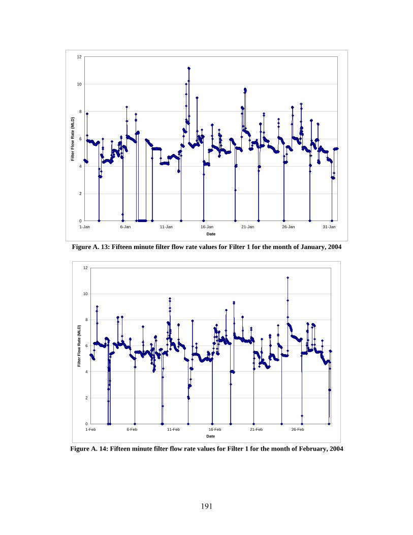
191
0
2
4
6
8
10
12
1-Jan 6-Jan 11-Jan 16-Jan 21-Jan 26-Jan 31-Jan
Date
Filte
r Flo
w R
ate
(MLD
)
Figure A. 13: Fifteen minute filter flow rate values for Filter 1 for the month of January, 2004
0
2
4
6
8
10
12
1-Feb 6-Feb 11-Feb 16-Feb 21-Feb 26-Feb
Date
Filte
r Flo
w R
ate
(MLD
)
Figure A. 14: Fifteen minute filter flow rate values for Filter 1 for the month of February, 2004

192
0
2
4
6
8
10
12
14
1-Mar 6-Mar 11-Mar 16-Mar 21-Mar 26-Mar 31-Mar
Date
Filte
r Flo
w R
ate
(MLD
)
Figure A. 15: Fifteen minute filter flow rate values for Filter 1 for the month of March, 2004
0
2
4
6
8
10
12
1-Apr 6-Apr 11-Apr 16-Apr 21-Apr 26-Apr 1-May
Date
Filte
r Flo
w R
ate
(MLD
)
Figure A. 16: Fifteen minute filter flow rate values for Filter 1 for the month of April, 2004

193
0
2
4
6
8
10
12
1-May 6-May 11-May 16-May 21-May 26-May 31-May
Date
Filte
r Flo
w R
ate
(MLD
)
Figure A. 17: Fifteen minute filter flow rate values for Filter 1 for the month of May, 2004
0
2
4
6
8
10
12
14
16
18
1-Jun 6-Jun 11-Jun 16-Jun 21-Jun 26-Jun 1-Jul
Date
Filte
r Flo
w R
ate
(MLD
)
Figure A. 18: Fifteen minute filter flow rate values for Filter 1 for the month of June, 2004

194
0
2
4
6
8
10
12
14
16
1-Jul 6-Jul 11-Jul 16-Jul 21-Jul 26-Jul 31-Jul
Date
Filte
r Flo
w R
ate
(MLD
)
Figure A. 19: Fifteen minute filter flow rate values for Filter 1 for the month of July, 2004
0
2
4
6
8
10
12
14
16
1-Aug 6-Aug 11-Aug 16-Aug 21-Aug 26-Aug 31-Aug
Date
Filte
r Flo
w R
ate
(MLD
)
Figure A. 20: Fifteen minute filter flow rate values for Filter 1 for the month of August, 2004

195
0
2
4
6
8
10
12
14
1-Sep 6-Sep 11-Sep 16-Sep 21-Sep 26-Sep 1-Oct
Date
Filte
r Flo
w R
ate
(MLD
)
Figure A. 21: Fifteen minute filter flow rate values for Filter 1 for the month of September, 2004
0
2
4
6
8
10
12
14
1-Oct 6-Oct 11-Oct 16-Oct 21-Oct 26-Oct 31-Oct
Date
Filte
r Flo
w R
ate
(MLD
)
Figure A. 22: Fifteen minute filter flow rate values for Filter 1 for the month of October, 2004

196
0
2
4
6
8
10
12
1-Nov 6-Nov 11-Nov 16-Nov 21-Nov 26-Nov 1-Dec
Date
Filte
r Flo
w R
ate
(MLD
)
Figure A. 23: Fifteen minute filter flow rate values for Filter 1 for the month of November, 2004
0
2
4
6
8
10
12
14
1-Dec 6-Dec 11-Dec 16-Dec 21-Dec 26-Dec 31-Dec
Date
Filte
r Flo
w R
ate
(MLD
)
Figure A. 24: Fifteen minute filter flow rate values for Filter 1 for the month of December, 2004
197
APPENDIX B: FULL CUMULATIVE DISTRIBUTION FUNCTIONS FOR ALL SIMULATOINS AND SIMULATION COMPARISONS

198
0.00
0.20
0.40
0.60
0.80
1.00
0.00 0.50 1.00 1.50 2.00 2.50 3.00
Turbidity (NTU)
Cum
ulat
ive
Prob
abili
ty (P
i)
Measured EffluentCFA Simulated Effluent
Figure B. 1: Comparison between measured turbidity effluent and CFA simulated effluent: Associated with
Figure 4.8
0.00
0.20
0.40
0.60
0.80
1.00
0.00 0.50 1.00 1.50 2.00 2.50 3.00
Turbidity (NTU)
Cum
ulat
ive
Prob
abili
ty (P
i)
Original CFAConditional Reliability CFA
Figure B. 2: Comparison between CFA and CFA modified for conditional reliability: Associated with Figure
4.12

199
0.00
0.20
0.40
0.60
0.80
1.00
0.00 0.50 1.00 1.50 2.00 2.50 3.00
Turbidity (NTU)
Cum
ulat
ive
Prob
abili
ty (P
i)
Original CFACFA January DataCFA May DataCFA September DataCFA January - June Data
Figure B. 3: Comparison the original CFA to CFA with sub-sets of data using cumulative distribution
functions: Associated with Figure 4.13
0.00
0.20
0.40
0.60
0.80
1.00
0.00 0.20 0.40 0.60 0.80 1.00 1.20 1.40 1.60
Effluent Turbidity (NTU)
Cum
ulat
ive
Prob
abili
ty (P
i)
CalibratedModel withRandom FilterFlow Rate
CalibratedModel withTime-SeriesFilter Flow Rate
Figure B. 4: Comparison of the CDF output from the probabilistic risk assessment for the calibrated OTTER
models with and without using a time series: Associated with Figure 5.14

200
0.00
0.20
0.40
0.60
0.80
1.00
0.00 0.50 1.00 1.50 2.00 2.50 3.00 3.50
Effluent Turbidity (NTU)
Cum
ulat
ive
Prob
abili
ty (P
i)
Measured Effluent
Calibrated Modelwith Random FilterFlow Rate
CFA Simulation
Figure B. 5: CDF of the output from the different risk analysis methodologies and the measured effluent:
Associated with Figure 6.4

201
APPENDIX C: PRELIMINARY ANALYSIS WITH THE OTTER FILTRATION MODEL

202
C.1 Preliminary Experiments with the OTTER Model
The OTTER filter model developed to undertake the preliminary experiments used static that
was consistent with the basic characteristics of the Brantford WTP, but without any of the
calibration that would be necessary for a full system analysis. Other parameters such as media
voidage and sphercity were kept as their default values from the OTTER software model itself.
The static data as used in the analysis can be seen in Figure C. 1.
Figure C. 1: OTTER static data for preliminary analysis
Operating data was also inputed and this data was kept close to model defaults. One change was
made with respect to the backwash triggers. An automatic backwash trigger of 2.20 m headloss
was used, from discussion with the Brantford WTP staff. Furthermore, 1.0 NTU backwash
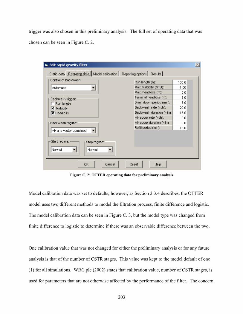
203
trigger was also chosen in this preliminary analysis. The full set of operating data that was
chosen can be seen in Figure C. 2.
Figure C. 2: OTTER operating data for preliminary analysis
Model calibration data was set to defaults; however, as Section 3.3.4 describes, the OTTER
model uses two different methods to model the filtration process, finite difference and logistic.
The model calibration data can be seen in Figure C. 3, but the model type was changed from
finite difference to logistic to determine if there was an observable difference between the two.
One calibration value that was not changed for either the preliminary analysis or for any future
analysis is that of the number of CSTR stages. This value was kept to the model default of one
(1) for all simulations. WRC plc (2002) states that calibration value, number of CSTR stages, is
used for parameters that are not otherwise affected by the performance of the filter. The concern

204
during this analysis is with turbidity removal, which is directly affected by the performance of
the filter as can be seen in Section 3.3.4, thus according WRC plc (2002) the number of CSTR
stages was did not need to be changed. This assumption was checked using two identical
simulations with CSTR numbers of one (1) and ten (10). The outputs from both simulations
were identical, thus the comments in WRc plc (2002) were verified and the number of CSTR
stages was not modified for any future simulations.
Figure C. 3: OTTER model calibration data for preliminary analysis
C.2 Comparison Between the Logistic Model, the Finite Difference
Model, and Measured Data using an Uncalibrated OTTER Model
C.2.1 Input Data Record
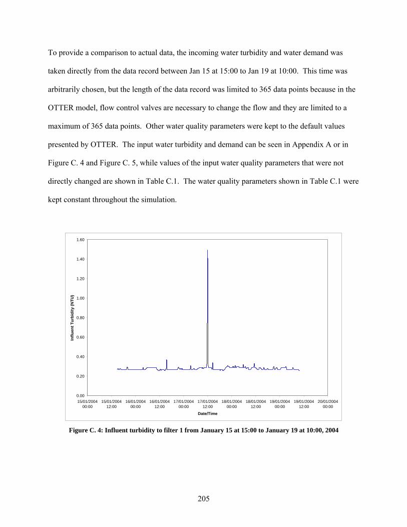
205
To provide a comparison to actual data, the incoming water turbidity and water demand was
taken directly from the data record between Jan 15 at 15:00 to Jan 19 at 10:00. This time was
arbitrarily chosen, but the length of the data record was limited to 365 data points because in the
OTTER model, flow control valves are necessary to change the flow and they are limited to a
maximum of 365 data points. Other water quality parameters were kept to the default values
presented by OTTER. The input water turbidity and demand can be seen in Appendix A or in
Figure C. 4 and Figure C. 5, while values of the input water quality parameters that were not
directly changed are shown in Table C.1. The water quality parameters shown in Table C.1 were
kept constant throughout the simulation.
0.00
0.20
0.40
0.60
0.80
1.00
1.20
1.40
1.60
15/01/200400:00
15/01/200412:00
16/01/200400:00
16/01/200412:00
17/01/200400:00
17/01/200412:00
18/01/200400:00
18/01/200412:00
19/01/200400:00
19/01/200412:00
20/01/200400:00
Date/Time
Influ
ent T
urbi
dity
(NTU
)
Figure C. 4: Influent turbidity to filter 1 from January 15 at 15:00 to January 19 at 10:00, 2004
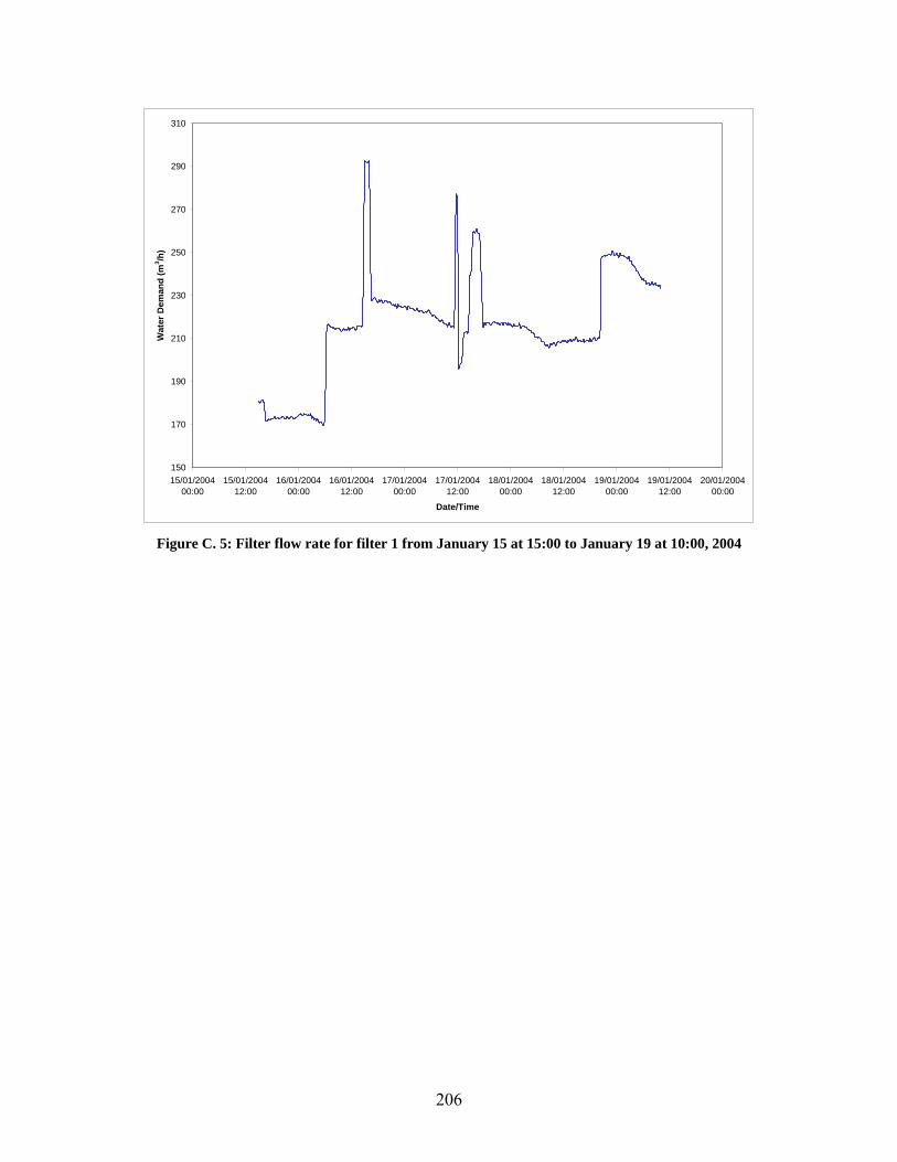
206
150
170
190
210
230
250
270
290
310
15/01/200400:00
15/01/200412:00
16/01/200400:00
16/01/200412:00
17/01/200400:00
17/01/200412:00
18/01/200400:00
18/01/200412:00
19/01/200400:00
19/01/200412:00
20/01/200400:00
Date/Time
Wat
er D
eman
d (m
3 /h)
Figure C. 5: Filter flow rate for filter 1 from January 15 at 15:00 to January 19 at 10:00, 2004

207
Table C. 1: Water quality parameters used in OTTER model
Parameter Amount Parameter Amount Parameter Amount pH 7.5 Nitrate 0 Chlortoluron (µg/L) 0
Temperature (oC)
15 Nitrite 0 Diuron (µg/L) 0
Apparent Colour
(oHazen)
50 Chloride 0 Isoproturon (µg/L) 0
True Colour 20 Chlorite 0 MCPA (µg/L) 0 Hardness (mg/L as CaCO3)
150 Chlorate 0 MCPB (µg/L) 0
Alkalinity (mg/L as CaCO3)
100 Bromide (mg/L) 0 Mecoprop (µg/L) 0
Conductivity (µS/cm)
400 Bromate (mg/L) 0 2,4-D (µg/L) 0
Total Suspended
Solids (mg/L)
Solids:Turbidity Ratio set at 2
Sulphate (mg/L) 0 Diazinon (µg/L) 0
Settleable Suspended
Solids (mg/L)
95% of the total suspended solids
Dissolved Oxygen (mg/L)
0 Chlorfenvinphos (µg/L)
0
Filtereable Suspended
Solids (mg/L)
95% of the total suspended solids
Orthophosphate (mgP/L)
0 Propetamphos (µg/L)
0
Free Chlorine (mg/L)
0 UV Adsorbance at 254 nm (/m)
12 Cysts (number/L) 0
Combined Chlorine (mg/L)
0 Total Organic Carbon (mg/L)
5 Coliforms (number/mL)
0
Chlorine Dioxide (mg/L)
0 Dissolved Organic Carbon (mg/L)
3 E. coli (number/mL)
0
Total Aluminium
(mg/L)
0 Particulate Organic Carbon (mg/L)
2 Viruses (number/mL)
0
Total Iron (mg/L)
0 Trihalomethanes (µg/L)
0 Heterotrophs (number/mL)
0
Total Manganese
(mg/L)
0 Trihalomethane Formation Potential
(µg/L)
0 Algae (cells/mL) 0
Dissolved Aluminium
(mg/L)
0 Haloacetic Acids (µg/L)
0 Chlorophyll-A (µg/L)
0
Dissolved Iron (mg/L)
0 Assimilable Organic Carbon (µg/L)
0 Taste (number) 0
Dissolved Manganese
(mg/L)
0 Atrazine (µg/L) 0 Odour (number) 0
Ammonia (mg/L)
0 Simazine (µg/L) 0 Particle Size 2

208
C.2.2 Output from OTTER Models
The effluent turbidity from the two models is shown in Figure C. 6, while the headloss within the
filter is shown in Figure C. 7. The output from the two models and the comparison between the
two model types is not meant to show which model best represents the data, but to show that the
different calculation mechanisms between the logistic and the finite difference models cause
differences in uncalibrated outputs. It also shows that calibration is necessary to accurately
represent a system, regardless of the model type that is used. Furthermore, the lower headloss
and higher effluent turbidity values shown by both models in Figure C. 6, Figure C. 7 and Table
C. 2 with respect to actual measurements makes sense because if the attachment efficiency was
increased, through calibration, the headloss would increase and more particles would be removed
by the filtration process. It was decided to use the logistic model for future simulations and
calibration, primarily for the simplicity of its use.
0.00
0.10
0.20
0.30
0.40
0.50
0.60
15/01/200400:00
15/01/200412:00
16/01/200400:00
16/01/200412:00
17/01/200400:00
17/01/200412:00
18/01/200400:00
18/01/200412:00
19/01/200400:00
19/01/200412:00
20/01/200400:00
Date/Time
Efflu
ent T
urbi
dity
(NTU
)
Measured DataLogistic Model Finite Difference Model
Figure C. 6: Comparison between output from uncalibrated OTTER models and measured effluent turbidity

209
0.00
0.50
1.00
1.50
2.00
2.50
15/01/200400:00
15/01/200412:00
16/01/200400:00
16/01/200412:00
17/01/200400:00
17/01/200412:00
18/01/200400:00
18/01/200412:00
19/01/200400:00
19/01/200412:00
20/01/200400:00
Date/Time
Filte
r Hea
dlos
s (m
)
Measured DataLogistic Model Finite Difference Model
Figure C. 7: Comparison between output from uncalibrated OTTER models and measured headloss
Table C. 2: Summary of output from simulations with Sub-Sets of the 2004 Data
Measured Effluent (NTU)
Logistic Model Effluent (NTU)
Finite Difference Model Effluent
(NTU) Maximum Turbidity 0.04 0.53 0.10 Minimum Turbidity 0.01 0.01 0.02 Turbidity Standard Deviation
0.01 0.03 0.01
Average Turbidity 0.01 0.01 0.04 Turbidity 95% Confidence
0.02 0.02 0.06
Turbidity 99 % Confidence
0.02 0.02 0.07
Measured Effluent (m)
Logistic Model Effluent (m)
Finite Difference Model Effluent (m)
Maximum Headloss 1.94 0.77 0.72 Minimum Headloss 0.50 0.26 0.26 Headloss Standard Deviation
0.41 0.13 0.12
Average Headloss 1.11 0.51 0.49
210
C.3 Effect of Changes in Input Water Quality on Model Outputs
C.3.1 Input Data Record
Although different water quality will ultimately change the output from a treatment system, a
preliminary test was carried out on the filtration system. This test was to see how the filter
effluent would change from a large change in the water quality characteristics that are not
directly associated with the filtration as described in the OTTER model. This meant changing
the water quality values that were described in Table C.1, Section C.2.1. Similar to the first
preliminary experiment, the water quality parameters, once changed, were kept constant during
the simulation. For comparison, the same water demand and influent turbidity profile as for the
first experiment was used. Table C. 3 shows the changed water quality inputs. Most of the
parameters described in Table C. 3 are expected to have little or no effect as they are not directly
related to the modelled filtration process described in Section 3.3.4.

211
Table C. 3: Changed water quality parameters used in the OTTER model
Parameter Amount Parameter Amount Parameter Amount pH 6 Nitrate 5 Chlortoluron (µg/L) 5
Temperature (oC)
10 Nitrite 5 Diuron (µg/L) 5
Apparent Colour
(oHazen)
100 Chloride 5 Isoproturon (µg/L) 5
True Colour 40 Chlorite 5 MCPA (µg/L) 5 Hardness (mg/L as CaCO3)
300 Chlorate 5 MCPB (µg/L) 5
Alkalinity (mg/L as CaCO3)
200 Bromide (mg/L) 5 Mecoprop (µg/L) 5
Conductivity (µS/cm)
800 Bromate (mg/L) 5 2,4-D (µg/L) 5
Total Suspended
Solids (mg/L)
Solids:Turbidity Ratio set at 2
Sulphate (mg/L) 5 Diazinon (µg/L) 5
Settleable Suspended
Solids (mg/L)
95% of the total suspended solids
Dissolved Oxygen (mg/L)
5 Chlorfenvinphos (µg/L)
5
Filtereable Suspended
Solids (mg/L)
95% of the total suspended solids
Orthophosphate (mgP/L)
5 Propetamphos (µg/L)
5
Free Chlorine (mg/L)
5 UV Adsorbance at 254 nm (/m)
24 Cysts (number/L) 100
Combined Chlorine (mg/L)
2 Total Organic Carbon (mg/L)
10 Coliforms (number/mL)
100
Chlorine Dioxide (mg/L)
2 Dissolved Organic Carbon (mg/L)
6 E. coli (number/mL)
100
Total Aluminium
(mg/L)
5 Particulate Organic Carbon (mg/L)
4 Viruses (number/mL)
100
Total Iron (mg/L)
5 Trihalomethanes (µg/L)
5 Heterotrophs (number/mL)
100
Total Manganese
(mg/L)
5 Trihalomethane Formation Potential
(µg/L)
5 Algae (cells/mL) 100
Dissolved Aluminium
(mg/L)
5 Haloacetic Acids (µg/L)
5 Chlorophyll-A (µg/L)
100
Dissolved Iron (mg/L)
5 Assimilable Organic Carbon (µg/L)
5 Taste (number) 100
Dissolved Manganese
(mg/L)
5 Atrazine (µg/L) 5 Odour (number) 100
Ammonia (mg/L)
4 Simazine (µg/L) 5 Particle Size 4

212
C.3.2 Output from OTTER Models
Table C. 4 outlines the results from the simulation after changing the input data. From Table C.
4 it can be seen that the turbidity effluent does not change with the changing water quality, but
that the water quality changes affect the headloss values. For future analysis, it should be noted
that introducing changes in the water quality can have an effect, depending on the input
parameter that is changed. However, further analysis was performed using the model defaults as
shown in Table C.1, Section C.2.1, noting that other water quality parameters could have some
effect.
Table C. 4: Summary of output from simulations with sub-sets of the 2004 data
Measured Effluent (NTU)
Logistic Model
Effluent (NTU)
Logistic Model Effluent New Water Quality
(NTU)
Finite Difference
Model Effluent (NTU)
Finite Difference Model Effluent
New Water Quality (NTU)
Maximum Turbidity
0.07 0.53 0.53 0.10 0.10
Minimum Turbidity
0.01 0.01 0.01 0.02 0.02
Turbidity Standard Deviation
0.01 0.03 0.03 0.01 0.02
Average Turbidity 0.01 0.01 0.01 0.04 0.04 Turbidity 95% Confidence
0.02 0.02 0.02 0.06 0.07
Turbidity 99 % Confidence
0.02 0.02 0.02 0.07 0.07
Measured Effluent (m)
Logistic Model
Effluent (m)
Logistic Model Effluent New Water Quality
(m)
Finite Difference
Model Effluent (m)
Finite Difference Model Effluent
New Water Quality (m)
Maximum Headloss
1.93 0.77 0.88 0.72 0.82
Minimum Headloss
0.50 0.26 0.30 0.26 0.30
Headloss Standard Deviation
0.41 0.13 0.15 0.12 0.14
Average Headloss 1.11 0.51 0.58 0.49 0.55

213
APPENDIX D: MODIFIED CALIBRATION PROCEDURE

214
The modified calibration procedure methodically looked at the different calibration parameters to
determine a combination of parameters that provided similar output to what was seen by the
measured turbidity effluent and headloss values in the 2004 data record.
It was necessary to compare the calibration parameters to the full data set; however, running each
set of calibration parameters through all 142 filter runs experienced in the 2004 year was not
practical or desirable. Therefore, the different combinations of calibration parameters were
assessed for their ability to model different runs chosen from the 2004 data record through a
linear optimization model. This linear optimization model was performed to find the most
“average” filter run and the filter runs that deviated from the “average” run the greatest.
A linear optimization model can be viewed as:
Minimize or Maximize ∑ jj xc Where xj is the parameter of interest And cj is the weight applied to the parameter. In terms of the model, the filtration process can be described by and is affected by a combination
of the turbidity influent, turbidity effluent, filter headloss and filter flowrate. An average filter
run would then be one that had an average turbidity influent, average turbidity effluent, average
headloss, and average filter flowrate over the filter run. To determine this specific filter run, the
median turbidity influent, turbidity effluent, filter headloss, and filter flowrate was calculated for
the 2004 year. The median values were then calculated for each filter run and the percent
difference between the filter run median and the overall median value was determined. The
average filter run was then determined using linear optimization, where the goal was to minimize
the percent difference over all four parameters. The linear optimization can be seen in Equation

215
17, where all ci values were equal to provide equal weighting to each parameter that could affect
the filtration process.
∑ +++ iiiiiiii FcHcEcIc
Equation 17
Where I is the percent difference in average turbidity influent from the run of interest to the
overall average, E is the percent difference in average turbidity effluent from the run of interest
to the overall average, H is the percent difference in average headloss from the run of interest to
the overall average, F is the percent difference in average filter rate from the run of interest to the
overall average.
Through this procedure, filter run 59 was found to be the most average filter run. The procedure
also allowed for the determination of the filter runs that deviated from the average the greatest
both above and below the median values provided absolute value differences were not used.
Thus the “high” filter run was determined to be filter run 80 and the “low” filter run was
determined to be filter run 31. Table D.1 shows the output from the analysis.
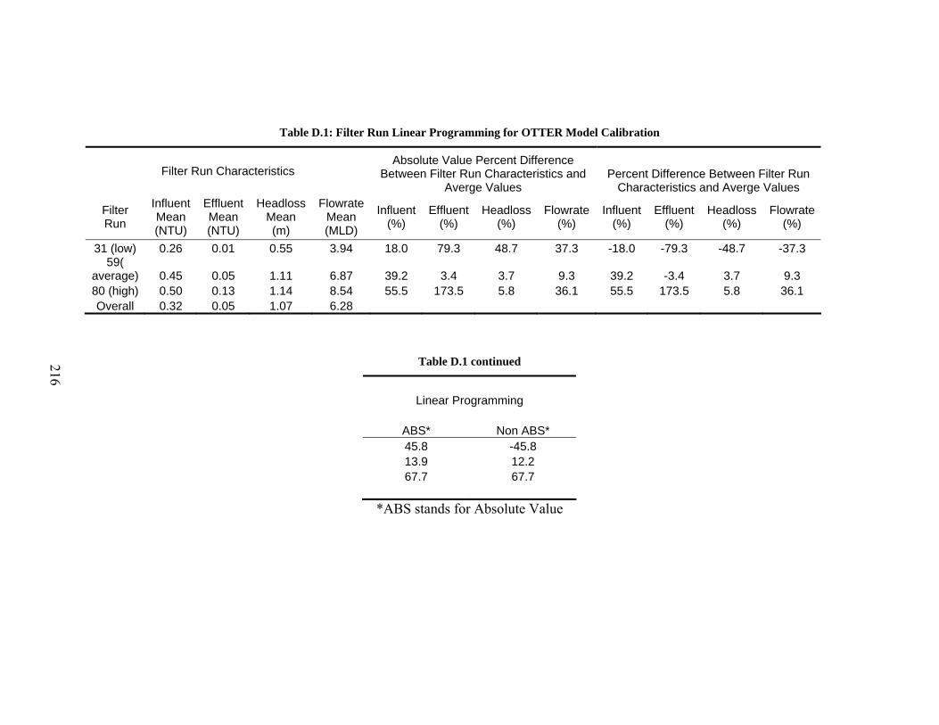
Table D.1: Filter Run Linear Programming for OTTER Model Calibration
Filter Run Characteristics Absolute Value Percent Difference
Between Filter Run Characteristics and Averge Values
Percent Difference Between Filter Run Characteristics and Averge Values
Filter Run
Influent Mean (NTU)
Effluent Mean (NTU)
Headloss Mean (m)
Flowrate Mean (MLD)
Influent (%)
Effluent (%)
Headloss (%)
Flowrate (%)
Influent (%)
Effluent (%)
Headloss (%)
Flowrate (%)
31 (low) 0.26 0.01 0.55 3.94 18.0 79.3 48.7 37.3 -18.0 -79.3 -48.7 -37.3 59(
average) 0.45 0.05 1.11 6.87 39.2 3.4 3.7 9.3 39.2 -3.4 3.7 9.3 80 (high) 0.50 0.13 1.14 8.54 55.5 173.5 5.8 36.1 55.5 173.5 5.8 36.1 Overall 0.32 0.05 1.07 6.28
Table D.1 continued
Linear Programming
ABS* Non ABS* 45.8 -45.8 13.9 12.2 67.7 67.7
*ABS stands for Absolute Value
216

217
The modified calibration procedure also took into account the accumulation within the filter. For
each filter run in 2004 the total amount of solids accumulated during the filter run was calculated
assuming the filters were clean at the start of each filter run. This allowed for the filter run
which caused the maximum amount of accumulation to be determined.
Visually, the ability of the calibrated model to duplicate the output from the 2004 data record can
be seen in Figure D.1 for the headloss and Figure D.2 for the effluent turbidity

0.0
0.5
1.0
1.5
2.0
2.5
0 10 20 30 40 50 60 70
Filter Run Time (hrs)
Filte
r Hea
dlos
s (m
)
Measured ValuesModel Values
0
0.1
0.2
0.3
0.4
0.5
0.6
0.7
0.00 2.00 4.00 6.00 8.00 10.00 12.00
Filter Run Time (hrs)
Filte
r Hea
dlos
s (m
)
Measured ValuesModel Values
0.0
0.2
0.4
0.6
0.8
1.0
1.2
1.4
1.6
1.8
0 20 40 60 80 100 120
Filter Run Time (hrs)
Filte
r Hea
dlos
s (m
)
Measured ValuesModel Values
0.0
0.5
1.0
1.5
2.0
2.5
0 5 10 15 20 25 30 35 40
Filter Run Time (hrs)
Filte
r Hea
dlos
s (m
)Measured ValuesModel Values
Figure D.1: Comparison of measured vales and model calculated values for filter headloss: Clockwise from top left, average filter run, low filter run,
high filter run, maximum accumulation filter run
218
Low Filter Run Average Filter Run
Maximum Accumulation Filter Run Average Filter Run

0.00
0.02
0.04
0.06
0.08
0.10
0.12
0 10 20 30 40 50 60 70
Filter Run Time (hrs)
Efflu
ent T
urbi
dity
(NTU
)
Measured ValuesModel Values
0
0.005
0.01
0.015
0.02
0.025
0.00 2.00 4.00 6.00 8.00 10.00 12.00
Filter Run Time (hrs)
Efflu
ent T
urbi
dity
(NTU
)
Measured ValuesModel Values
0.00
0.02
0.04
0.06
0.08
0.10
0.12
0 20 40 60 80 100 120
Filter Run Time (hrs)
Efflu
ent T
urbi
dity
(NTU
)
Measured ValuesModel Values
0.00
0.02
0.04
0.06
0.08
0.10
0.12
0.14
0.16
0.18
0.20
0 5 10 15 20 25 30 35 40
Filter Run Time (hrs)
Efflu
ent T
urbi
dity
(NTU
)
Measured ValuesModel Values
Figure D.2: Comparison of measured vales and model calculated values for filter effluent: Clockwise from top left, average filter run, low filter run,
high filter run, maximum accumulation filter run
219
Average Filter Run Low Filter Run
Maximum Accumulation Filter Run High Filter Run

220
APPENDIX E: YATE’S METHOD CALCULATIONS FOR PREDICTIVE MODELLING AND RISK ANALYSIS

Table E.1: Yate’s method for calculating effect estimates for the probability that the effluent turbidity is greater than 0.05 NTU
Simulation #
Filter Depth
(m)
Influent Turbidity (NTU)
Filter Flow Rate (MLD)
Probability > 0.05 NTU
(%) [1] [2] [3] Divisor Effect
Estimate Source 11 -1 -1 -1 4.84 0.0740 0.1515 0.1848 8 0.0231 Mean 13 -1 -1 1 2.56 0.0775 0.0333 -0.0584 4 -0.0146 Flow
12 -1 1 -1 4.91 0.0213 -0.0435 -0.0058 4 -0.0015 Turbidity
10 -1 1 1 2.84 0.0120 -0.0149 0.0078 4 0.0020 Flow x Turbidity
7 1 -1 -1 1.58 -0.0228 0.0035 -0.1182 4 -0.0296 Depth
9 1 -1 1 0.55 -0.0207 -0.0093 0.0286 4 0.0072 Flow x Depth
8 1 1 -1 0.83 -0.0103 0.0021 -0.0128 4 -0.0032 Depth x
Turbidity
6 1 1 1 0.37 -0.0046 0.0057 0.0036 4 0.0009 Flow x
Turbidity x Depth
Sum of Squares 0.0132 0.0263 0.0526
221
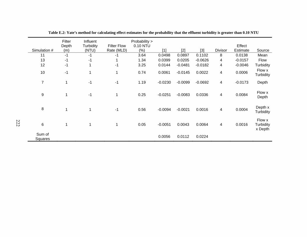
Table E.2: Yate’s method for calculating effect estimates for the probability that the effluent turbidity is greater than 0.10 NTU
Simulation #
Filter Depth
(m)
Influent Turbidity (NTU)
Filter Flow Rate (MLD)
Probability > 0.10 NTU
(%) [1] [2] [3] Divisor Effect
Estimate Source 11 -1 -1 -1 3.64 0.0498 0.0897 0.1102 8 0.0138 Mean 13 -1 -1 1 1.34 0.0399 0.0205 -0.0626 4 -0.0157 Flow 12 -1 1 -1 3.25 0.0144 -0.0481 -0.0182 4 -0.0046 Turbidity
10 -1 1 1 0.74 0.0061 -0.0145 0.0022 4 0.0006 Flow x Turbidity
7 1 -1 -1 1.19 -0.0230 -0.0099 -0.0692 4 -0.0173 Depth
9 1 -1 1 0.25 -0.0251 -0.0083 0.0336 4 0.0084 Flow x Depth
8 1 1 -1 0.56 -0.0094 -0.0021 0.0016 4 0.0004 Depth x
Turbidity
6 1 1 1 0.05 -0.0051 0.0043 0.0064 4 0.0016 Flow x
Turbidity x Depth
Sum of Squares 0.0056 0.0112 0.0224
222

TableE.3: Yate’s method for calculating effect estimates for the probability that the effluent turbidity is greater than 0.30 NTU
Simulation #
Filter Depth
(m)
Influent Turbidity (NTU)
Filter Flow Rate (MLD)
Probability > 0.30 NTU
(%) [1] [2] [3] Divisor Effect
Estimate Source 11 -1 -1 -1 1.95 0.0244 0.0423 0.0560 8 0.0070 Mean 13 -1 -1 1 0.49 0.0179 0.0137 -0.0392 4 -0.0098 Flow 12 -1 1 -1 1.6 0.0104 -0.0287 -0.0136 4 -0.0034 Turbidity
10 -1 1 1 0.19 0.0033 -0.0105 0.0052 4 0.0013 Flow x Turbidity
7 1 -1 -1 0.9 -0.0146 -0.0065 -0.0286 4 -0.0072 Depth
9 1 -1 1 0.14 -0.0141 -0.0071 0.0182 4 0.0046 Flow x Depth
8 1 1 -1 0.31 -0.0076 0.0005 -0.0006 4 -0.0002 Depth x Turbidity
6 1 1 1 0.02 -0.0029 0.0047 0.0042 4 0.0011 Flow x
Turbidity x Depth
Sum of Squares 0.0015 0.0030 0.0061
223