The use of Optimisation algorithms in PSO - NAFEMS · The use of Optimisation algorithms in PSO Prof. Carlo Poloni, University of Trieste, Dr. Valentino Pediroda, University of Trieste,

FENET THEMATIC NETWORK

COMPETITIVE AND SUSTAINABLE GROWTH (GROWTH) PROGRAMME

1

Industry Sector RTD Thematic Area Date Deliverable Nr

Product and System Optimization

28.04.2005 4

The use of Optimisation algorithms in PSO

Prof. Carlo Poloni, University of Trieste,

Dr. Valentino Pediroda, University of Trieste,

Dr. Alberto Clarich, University of Trieste

Prof. Grant Steven, University of Durham, UK

Summary: A general overview of how and when Optimisation Algorithms are applicable to product and systemdesign is here given. The document is intended as a first attempt to build guidelines for the best usageof PSO techniques. This report summarises the main discussions points related to RTD2 on Productand System Optimisation (PSO) raised at the FENET Workshop held in 2002 and summarized on27-28 February 2003, completed with the additional remarks defined at the FENET workshop held onMarch 2004, October 2004 and February 2005. This document serves as a brief introduction to the complex field of optimisation, as such it onlyprovides simple indications to the non-expert practitioner on which method to consider.



2

Introduction There is no single solution to design optimisation tasks. Many techniques are available and most of them have pro and cons. While in the well established world of “simulation” the principles are clear (build a model able to reproduce numerically the physics of a phenomenon), in the PSO arena the driving force should become “improve your available design”. There is a major difference in the two sentences: in the first case the “physics” is supposed known and the model should represent the reality within acceptable accuracy, i.e. the target is known and the method to reach it is subject to development, in the second case the model is assumed to be valid and improvements to the product performance are the target, i.e. the method is known and the target to be reached is not defined. It is therefore clear that it is not possible to define a-priori which is the best optimisation methodology but, by classifying the problems being addressed, it is possible to derive “rules of thumb” that can suggest to the engineer which strategy is likely the most efficient in giving performance improvements for a given optimisation problem. In this report we briefly classify and describe the main optimisation methods after a brief introduction on the basic terminology of optimisation. A “applicability table” is given, while a preliminary classification of benchmarks and application examples is described.

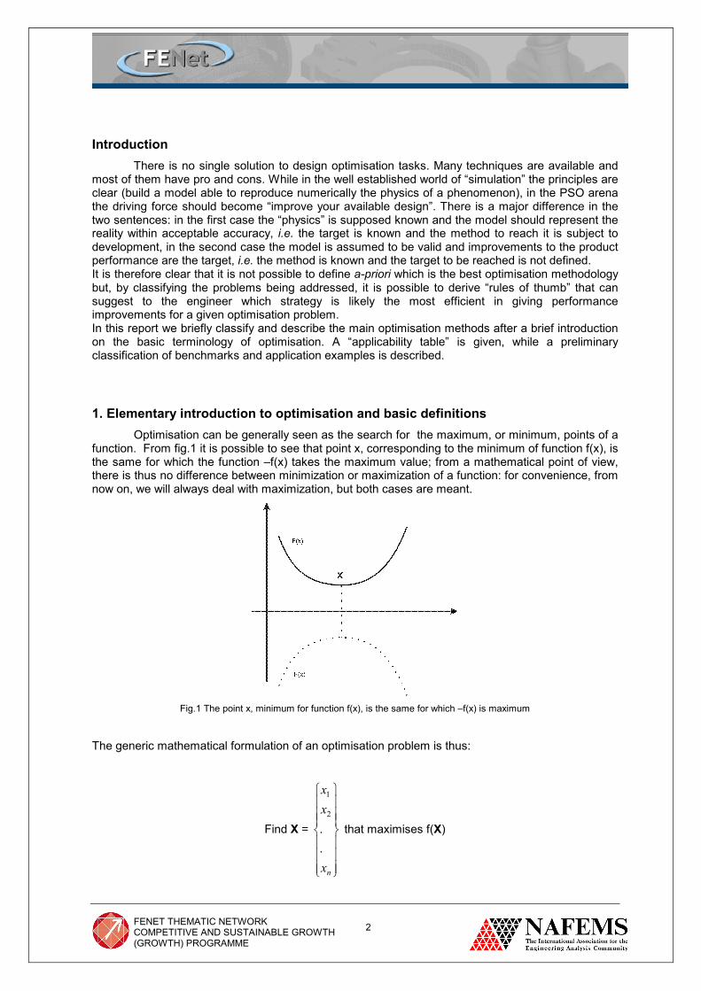
1. Elementary introduction to optimisation and basic definitions Optimisation can be generally seen as the search for the maximum, or minimum, points of a function. From fig.1 it is possible to see that point x, corresponding to the minimum of function f(x), is the same for which the function –f(x) takes the maximum value; from a mathematical point of view, there is thus no difference between minimization or maximization of a function: for convenience, from now on, we will always deal with maximization, but both cases are meant.

Fig.1 The point x, minimum for function f(x), is the same for which –f(x) is maximum

The generic mathematical formulation of an optimisation problem is thus:

Find X =

nx

xx

.

.2

1

that maximises f(X)



3

subjected to the constraints:

gj(X)<0, j=1,2,…..,m

lj(X)=0, j=1,2,…..,p

where X is an n-dimensional vector called vector of the design variables, f(X) is defined as the objective function, and the constraints gj(X), lj(X)are inequality constraints and equality constraints respectively. The latter problem is called constrained optimisation problem, while if the constraints are not present, the problem is called unconstrained optimisation problem.

A slightly more general formulation of an optimisation problem is the following:

Find X =

nx

xx

.

.2

1

that maximises fj(X) j=1,2,……,q;

The function to be optimised is now not unique, but there are q functions; this class of optimisation problems is called multi-objective optimisation and is a common type of optimisation in the engineering field.

1.1 Design variables vector Most of the engineering systems are defined by a set of quantities that can be modified during the project design. Some of these quantities are kept fixed and consequently are called assigned parameters; conversely, the remaining quantities that are variable during the project design, are called design variables, and can be set, from a mathematical point of view, in the

vector of design variables X =

nx

xx

.

.2

1

. It should be noted that these definition are not definitive, since

their role can be changed during the project design. For instance, during the project design of the rotor of a gas turbine, the blade number can be seen in an initial phase as a design variable, but, successively, when the optimal number is found, it becomes an assigned parameter. This demonstrates that an optimisation process is not obtained always in a single step, but it should be seen as a succession of steps, each of them linked with the previous one, during which the objectives and variables are modified until the best compromise is obtained.

1.2 Objective function An optimisation methodology is aimed to find a configuration of the analysed system that respects some conditions. Generally, the project design gives more than one configuration that satisfies the designer expectations and the aim of an optimisation process is then to find the configuration with the best features. Consequently, it is necessary to choice a criterion by which to compare each different configuration with the other ones: this criterion is called objective function or fitness function. The choice of the objective function depends on the nature of the optimisation problem; in the turbo-machinery, it may be the thermo-fluid-dynamic efficiency, in structural



4

mechanics the weight of the system, in finance the gain, etc. The definition of the objective fitness determines in a unique way the optimisation process.

The definition of the objective function is however not always trivial; if, for example, an aerodynamic profile is optimised for minimum drag resistance, the profile found will probably be characterised by an almost null lift force, a situation that cannot be accepted by the designer. In these cases it will be needed to define more objective functions (drag, lift) to be optimised simultaneously (at least in the initial phases of the optimisation, since in the final phases it is possible to select a single fitness function); this class of optimisation, that is common in the project design, is known as multi-objective optimisation. The classic way to solve this class of optimisation, given two functions f1(X) and f2(X), is to define the functional:

f(X)=α1 f1(X)+ α2 f2(X)

where α1 and α1 are constants that define the importance of an objective with respect to the other one. As will be shown, this approach is not the most adapt for the solution of multi-objective problems; for this reason new algorithms have been developed whose basic feature is the simultaneous optimisation of the objective functions, avoiding the use of a functional that reduces the problem from multi-objective to one that is single-objective.

1.3 Constraints In most common problems, it is necessary to define other functions beside the objective functions in order to obtain feasible solutions. For instance, in the case of structural optimisation, if the objective is the minimization of the weight of a structure, it will be necessary to check if the structure resists the loads (σmax<σadm). Such functions are known as constraints.

Generally, a constraint is given by a function of the type gj(X)<0, whose surface (gj(X)=0) divides the solutions space in two regions: one for which gj(X)<0 (space of admissible solutions) and its dual space gj(X)>=0 (space of inadmissible solutions).

In fig.2, we show a hypothetical 2-variables space, subject to three constraints g1(X), g2(X), g3(X). It should be noted that the maximum of the function found by the optimisation process is different, due to the presence of constraints, from the maximum of the unconstrained function that is located in the region of the inadmissible solutions for the constraint g1(X): in conclusion, the presence of constraints modifies the result of the optimisation.

Fig.2 Contours of objective function with 3 constraints g1(X), g2(X), g3(X)

During the last few years several methods have been proposed for handling constraints in heuristic optimisation algorithms. These methods can be grouped into two main categories: methods that preserve the feasibility of solutions and methods based on penalty functions. The methods that preserve the feasibility are quite efficient but are not always applicable. In fact the feasibility of the off-springs can be maintained only by the use of repairing techniques or by



5

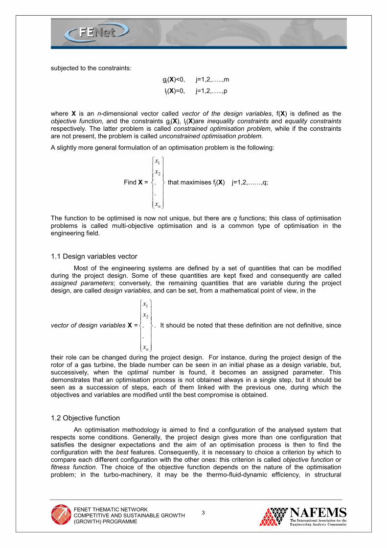
specialized cross-over operators (in the case of Genetic Algorithms) that are usually problem-dependent. Conversely, methods based on penalty functions employ the concept that the fitness function is decreased according to the intensity of the constraint violation. A drawback of this methodology is that the intensity of the penalisation can be problem-dependent and might cause the optimisation to converge prematurely. A way to overcome this problem is to adapt the penalty function to the current population under evaluation. Two possible methodologies suitable also for multi-objective optimisation are here described. The first way is to transform the numerical constraint into a fuzzy function (Fig. 2a)

Fig. 2a Penalty function

For all the objectives defined by index i, in case of maximization, the fitness functions are computed as follows, taking in account the contribution of each of the q constraints gj(x):

[ ]minmax

1

)()()(

jjj

q

jjjii

ffh

xgPhxfxFit

−=

−= ∑=

If g(x) is negative the individual is feasible and the algorithm works as in the case of unconstrained optimisation (P(g(x)=0), whereas if g(x) is greater than 0 the individual is worst than any feasible solution (because of parameter hj) and the number of violated constraints dominates the problem. In many engineering optimisation cases, there is the necessity of using a different approach in the constraints, that avoids a rigid distinction between feasible and infeasible solutions, with a tolerance for the constraints slightly violated: for this reason, a new approach, based on fuzzy functions, has been developed (Fig. 2b).



6

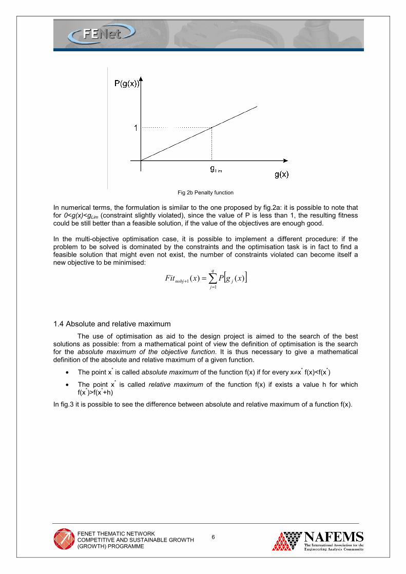
Fig 2b Penalty function

In numerical terms, the formulation is similar to the one proposed by fig.2a: it is possible to note that for 0<g(x)<gLim (constraint slightly violated), since the value of P is less than 1, the resulting fitness could be still better than a feasible solution, if the value of the objectives are enough good. In the multi-objective optimisation case, it is possible to implement a different procedure: if the problem to be solved is dominated by the constraints and the optimisation task is in fact to find a feasible solution that might even not exist, the number of constraints violated can become itself a new objective to be minimised:

[ ]∑=

+ =q

jjnobj xgPxFit

11 )()(

1.4 Absolute and relative maximum The use of optimisation as aid to the design project is aimed to the search of the best solutions as possible: from a mathematical point of view the definition of optimisation is the search for the absolute maximum of the objective function. It is thus necessary to give a mathematical definition of the absolute and relative maximum of a given function.

• The point x* is called absolute maximum of the function f(x) if for every x≠x* f(x)<f(x*)

• The point x* is called relative maximum of the function f(x) if exists a value h for which f(x*)>f(x*+h)

In fig.3 it is possible to see the difference between absolute and relative maximum of a function f(x).



7

Fig.3 A1:absolute maximum, A2:relative maximum

1.5 Robustness of an optimisation algorithm The distinction between absolute and relative maximum of a function is very important to determine the robustness of an optimisation algorithm. In fact robustness may be defined as the capability of an optimisation algorithm to find the absolute maximum of the objective function. This is one of the most important feature for the efficiency of an optimisation methodology: higher is the robustness of an algorithm and higher will be the probability to find the absolute maximum of a function. We have used the expression probability since no algorithm can assure a priori that the optimal solution found is really the absolute maximum of the given function.

From the definition of robustness, it is possible to indicate some common features of the optimisation algorithms. There exist two main classes of algorithms: the ones that use the gradient of the objective function and the ones that use only the value of the function. The use of the gradient of the objective function proceeds, in the simplest case, as follows:

• Choose a X0 point to start the optimisation

• Calculate of the partial derivatives ix

f∂∂

, i=1,...,n

• Calculate of new point i

ni

ni x

fxx∂∂+= − )1()( i=1,...,n

• Return to point 2 until ε<∇f , with any ε given.

This approach to optimisation has the problem of being less robust because it is local. In fact, as shown in fig.4, for this kind of problems the choice of the starting point X0 is very important, since the solution found will be the relative maximum closest to the starting point, and will therefore not necessarily correspond to the absolute maximum of the objective function.



8

Fig.4 Local optimisation algorithm: starting from P1 leads to absolute maximum M1, starting from P2 leads to

relative maximum M2

In conclusion, to use optimisation algorithms based on the calculation of the objective function gradient, it will be necessary to perform a series of successive optimisations, changing each time the starting point.

1.6 Accuracy of an optimisation algorithm Beside the concept of robustness, it is important to define the concept of accuracy. Observing fig.5, it is possible to note that the final solution of two different optimisation algorithms may differ more or less from the maximum of the given function.

Fig.5 Two optimisation algorithms: the one on left finds a solution closer to function maximum than the one on right

Consequently, the accuracy of an algorithm is defined as its capability to find a solution the most possible close to the absolute (absolute or relative) of the given function.

Usually, an optimisation algorithm is not both robust and accurate: the ability to find the absolute maximum of a function is not linked to the ability to find a solution as close as possible to the ideal one. For example, genetic algorithms present a good robustness but a poor accuracy, whereas the opposite is for gradient-based methods. Consequently, the choice of the optimisation algorithm should not be done a priori, but should be done with reference to each particular problem. We can indicate some simple guidelines:

• If the project design requires the improvement of an existing solution, it will be useful to use an accurate algorithm, possibly based on the gradient, because the existence of a good

P2

M2



9

solution provides a basis for improvement, moving in the direction of the closest relative maximum;

• If on the contrary it is required a solution ab-initio, it will be more convenient to use a robust methodology, in order to create a set of solutions as closest as possible to the absolute maximum of the function.

The use of hybrid optimisation algorithms offers interesting possibilities, since they use more algorithms in series or in parallel. A classic methodology is to start with a robust algorithm and then, using the obtained solution as new starting point, to apply an accurate algorithm; in this way it is possible to fully take advantage of the best features of the algorithms (robustness + accuracy), finding the best solution as possible. As will be seen more over, this methodology is particularly efficient when genetic algorithms (robustness), gradient-based methods (accuracy) and methodologies for response surfaces are all linked together.

1.7 Parameterisation Deeply related to the definition of design variables is the concept of parameterisation. In fact, as previously observed, the design variables are the values that define the engineering system: they can be geometric quantities (dimension), measures of physical properties (velocity, pressure) and anything else needed to define the given system. These quantities are variable during the project design and the modification of the system produced by their variation is defined as parameterisation. The most common parameterisation is geometric, in which the design variables influence the geometry of the system, since commonly it is required to find the geometric configuration that guarantees the best performances. In fig.6 we report, as an example, the case of the geometric parameterisation of the camber line of a turbo-machine blade.

Fig.6 Example of geometric parameterisation: camber line of turbomachine is modified by the parameters A1 and A2 (angles)

The definition of the parameterisation is one of the most important phases in the optimisation process, since the best solution will be limited to the configurations defined by the chosen parameterisation, that does not necessarily consider all the possible configurations of the given system. The most frequent problems that can happen are:

• “poor” parameterisation

• “redundant” parameterisation

In the first case it can happen that the adopted parameterisation does not include the optimum configuration of the system: this is a very frequent case and is very difficult to identify, since it is



10

impossible to know a priori the optimum configuration of the system. To avoid this situation one of the approaches adopted is to try the inverse design of several good optimal configurations. For example, in the parameterisation of aerodynamic profiles, it is recommended that the design f parameterisation,is based upon commonly used profiles.

Conversely, in the case of redundant parameterisation, there are too many variables to define the features of the system; in this way the most influential parameters are penalised and the optimisation is greatly slowed down from a numerical point of view (the problems defined by more variables requires normally a larger computational cost to reach the optimal solution).

2. Classification of Optimisation methods

2.1 Integer / Discrete / Linear programming Integer/Discrete/Linear programming is used when it is possible to express a mathematical

function of the variables (that take only integer values) and to define some mathematical constraints. In that case, it is possible to represent the equations by simple geometrical entities like lines or planes, and to find graphically the solution by the intersection of the constraints and the equations to be maximised on the grid of discrete points. The applicability of these methods is however limited to few particular cases, since in most industrial cases it is not possible to have simple linear equations that describe the process.

Fig.7 Example of Integer Programming for optimisation of discrete variables 2.2 Downhill Simplex

The Nelder and Mead Downhill Simplex is a single-objective optimisation algorithm particularly efficient for not highly non-linear optimisation cases and for continuous variables.

The algorithm needs an initial set of n+1 configurations, n being the number of variables, and it optimises the objective through m following iterations. We indicate each configuration by the vector point of variables xi=(xi

1,xi2,….,xi

n). At each step, the worst configuration, that we call xn+1, is replaced by a new configuration, xN

n+1, that is obtained by the geometric projection of the point xn+1 with respect to the plane π defined by the other n (x1,…,xn) points of the initial set.

Optimised point



11

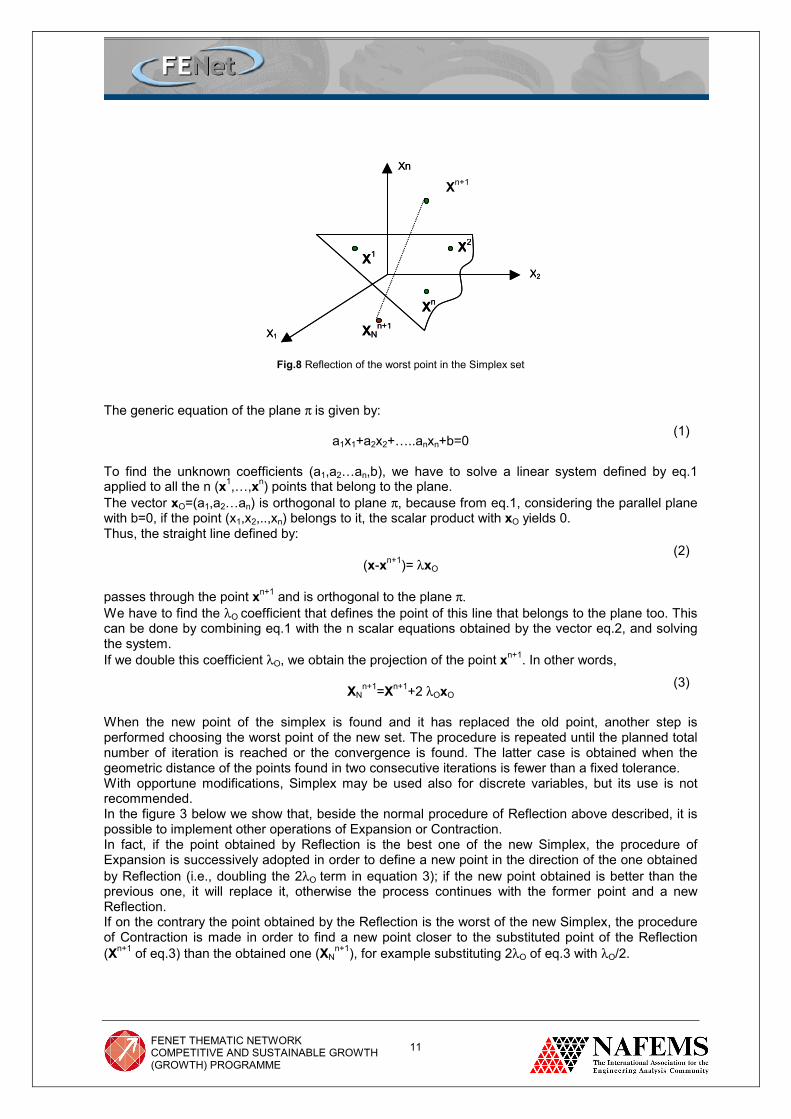
Fig.8 Reflection of the worst point in the Simplex set The generic equation of the plane π is given by:

a1x1+a2x2+…..anxn+b=0

To find the unknown coefficients (a1,a2…an,b), we have to solve a linear system defined by eq.1 applied to all the n (x1,…,xn) points that belong to the plane. The vector xO=(a1,a2…an) is orthogonal to plane π, because from eq.1, considering the parallel plane with b=0, if the point (x1,x2,..,xn) belongs to it, the scalar product with xO yields 0. Thus, the straight line defined by:

(x-xn+1)= λxO

passes through the point xn+1 and is orthogonal to the plane π. We have to find the λO coefficient that defines the point of this line that belongs to the plane too. This can be done by combining eq.1 with the n scalar equations obtained by the vector eq.2, and solving the system. If we double this coefficient λO, we obtain the projection of the point xn+1. In other words,

XNn+1=Xn+1+2 λOxO

When the new point of the simplex is found and it has replaced the old point, another step is performed choosing the worst point of the new set. The procedure is repeated until the planned total number of iteration is reached or the convergence is found. The latter case is obtained when the geometric distance of the points found in two consecutive iterations is fewer than a fixed tolerance. With opportune modifications, Simplex may be used also for discrete variables, but its use is not recommended. In the figure 3 below we show that, beside the normal procedure of Reflection above described, it is possible to implement other operations of Expansion or Contraction. In fact, if the point obtained by Reflection is the best one of the new Simplex, the procedure of Expansion is successively adopted in order to define a new point in the direction of the one obtained by Reflection (i.e., doubling the 2λO term in equation 3); if the new point obtained is better than the previous one, it will replace it, otherwise the process continues with the former point and a new Reflection. If on the contrary the point obtained by the Reflection is the worst of the new Simplex, the procedure of Contraction is made in order to find a new point closer to the substituted point of the Reflection (Xn+1 of eq.3) than the obtained one (XN

n+1), for example substituting 2λO of eq.3 with λO/2.

XNn+1

Xn

X2

X1

Xn+1

X1

X2

Xn

(1)

(2)

(3)

XNn+1

Xn

X2

X1

Xn+1

X1

X2

Xn



12

Fig.9 Operations on the Simplex

2.3 Gradient based methods The Gradient-based methods are applicable only in single-objective cases, but they are

recommended to be used particularly for refinement purposes (high accuracy) or/and in combination with RSM methods, for the high number of calculations required, and for the reason that they have some difficulties to find the global maximum (low robustness), since they operate locally. In fact, the simplest algorithm is are based on the iterative search of an improved point, moving in the direction of the gradient of the function calculated at the previous point (or in the opposite direction if the function is to be minimised); this direction is called direction of maximum increment, since the gradient indicates the direction where the variation of the function is maximum. The gradient of a function f(x1,..xn) is defined by:

The partial derivatives, when there is not a mathematic formulation or are not given directly by a computational code, may be approximated in the most efficient way by the methodology of finite difference, that can be defined in two different ways. The first definition, called upwind approximation, is shown in eq.5a, while the second, central approximation, is shown by eq.5b:

The second definition of finite difference is more accurate, but, while the upwind approximation requires n further evaluations of function f(X) (one for each partial derivative, from the term ( )iim xf uX ∆+ ), the central approximation requires 2n evaluations.

In these formulas, ui the ith versor, and ∆xi is chosen appropriately: if it is too big, the numeral approximation of the derivatives may not be sufficiently accurate, while if it is too small, the finite difference may be affected by the round-off error introduced by the computer.

( ) ( )ni

xfxf

xf

i

miim

im

,...,1=∆

−∆+≅

XuX

x∂∂ (5a)

Initial Simplex

Reflection

Reflection and Expansion

Contraction

( ) ( )ni

xxfxf

xf

i

iimiim

im

,...,12

=∆

∆−−∆+≅

uXuX

x∂∂

(5b)

(4)

=∇

nxf

xfxf

f

∂∂

∂∂∂∂

/

//

2

1

Μ(4)

:



13

It is important to note that not always it is possible to define the gradient of a function in some points; a function may be non- differentiable at a point if, for example, the function is not continuous, or if it is not regular (the derivative at left is different from derivative at right in that point). The gradient cannot be calculated in the case of discrete variables also, for this reason the gradient-based methods can only be applied with real variables.

In conclusion, the gradient-based methods suffer from the following defects:

• Need of large quantities of further calculations for the definition of partial derivatives by finite difference approximation (if derivatives are not known analytically or obtained directly by the solver)

• Impossibility of application in some cases (discrete variables, function discontinuous or non-differentiable)

• Low robustness of the algorithm

There are several algorithms that are based on the gradient method, like Cauchy, Newton, quasi-Newton, BFGS, Powell, SPQ, Conjugate Gradient, etc. We describe briefly the most important methods

2.3.1 Cauchy method The methodology is iterative, and can be defined as follows:

• Start from initial point X1

• Calculation of direction S1 = ∇ f(X1)

• Calculation of new point X1+1 using optimal step λi* in direction S1

X1+1= X1+ λi* S1

• If convergence satisfied, ends, otherwise, continues from point 2.

The convergence occurs when the relative variation of the function or the variables vector over two successive steps is smaller than a fixed constant: or the values of the partial derivatives are close to zero,

)f(X)f(X-)X-f(X|

i

ii1i+ <ε1

ii XX −+1 <ε2

ixf

∂∂

<ε3

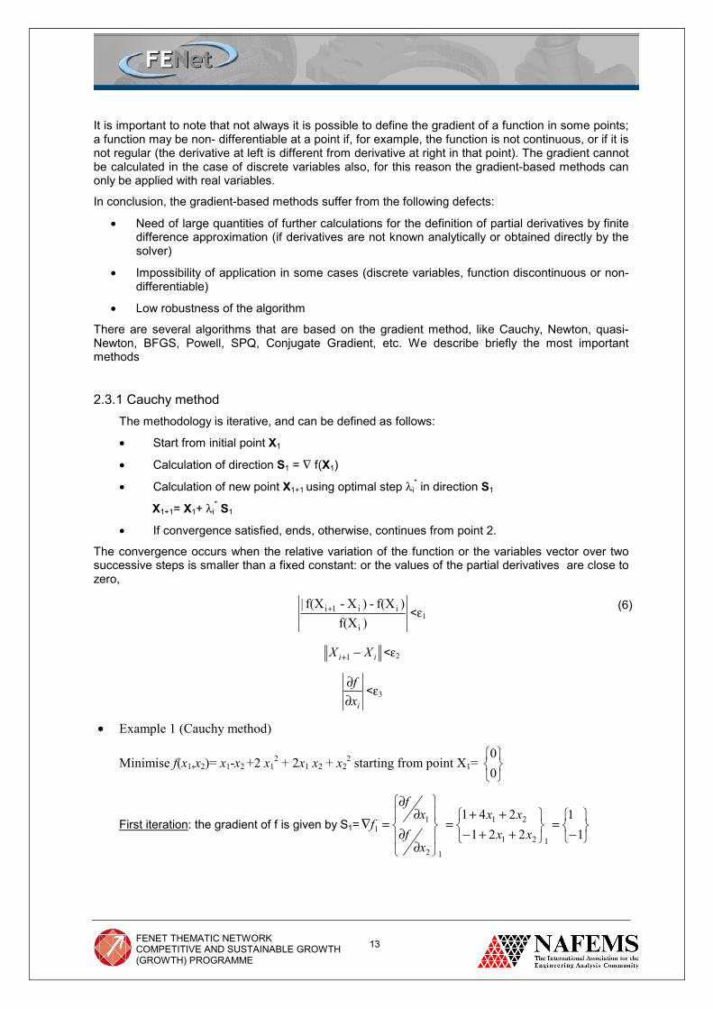
• Example 1 (Cauchy method)

Minimise f(x1,x2)= x1-x2 +2 x12 + 2x1 x2 + x2

2 starting from point X1=

00

First iteration: the gradient of f is given by S1=

−=

++−++

=

∂∂

∂∂

=∇1

1221

241

121

21

12

11 xx

xx

xf

xf

f

(6)



14

The optimal step for the calculation of X2 is found by the minimization of f(X1,X1-λS1)= λ2−2 λ,

with respect to λ, that gives λ1=1; in this way, X2=X1-λS1=

00

-1

−11

=

−1

1

To consider if X2 is optimum, we have to check if f∇ (x2)=

00

or not; in this case, it is

−−

11

,

so need to proceed with the next iteration.

Second iteration: S2= f∇ 2=

−−

11

, while the optimal step λ2 is obtained by the minimisation of

f(X2,X2-λS2)= 5λ2+2 λ−1, that gives λ2=−1/5; in this way X3=

−1

1-1/5

−−

11

=

−

2.18.0

The gradient in the new point gives

− 2.02.0

, thus we need another iteration

Third iteration: S3= f∇ 3=

− 2.02.0

, while the optimal step λ3 is obtained by the minimisation of

f(X3,X3-λS3), that gives λ3=−1.0; in this way X4=-

−

2.18.0

-1

− 2.02.0

=

−

4.10.1

The gradient in the new point gives

−−

2.02.0

, thus we need another iteration; the process is

continued until the convergence is found at the point X*=

−

5.10.1

.

2.3.2 Newton method

The Newton method is very efficient, especially in the case of quadratic functions, In this latter case, only a single iteration is required for the convergence of the algorithm.

It is possible to approximate a function in a point Xi through the Taylor series as follows:

[ ] )()(21)()()( ii

Tii

Tii XXJXXXXfXfXf −−+−∇+=

where [ ]iJ = [ ]ix

J is the matrix of second order derivatives (the Hessian) calculated at the point Xi.

The necessary condition, for which the point Xi is a maximum for the function, is given by ∇fi=0; in that case, if we calculate the gradient of eq.7, we obtain:

[ ] )(00)( ii XXJXf −++=∇

If [ ]iJ is not singular, it is possible to calculate a new point Xi+1 from eq.8 as follows:

[ ] iiii fJXX ∇−= −+

11

Of course, eqs.8 and 9 will be applied on the new point Xi+1 more times iteratively, until the convergence, that is obtained when Xi+1 is the maximum of the function and satisfies the condition ∇fi=0: in that case, from eq.9 it will follow that Xi+1=Xi, and the algorithm stops. If the function is not quadratic (in that case only one step is required for convergence), eq.9 may be modified, to

(7)

(8)

(9)



15

increment the robustness of the algorithm and to reduce the total number of iterations required, by introducing an optimal step of variation λi

*:

[ ] iiiii fJXX ∇−= −+

1*1 λ

The difficulty of this methodology in practice, is the calculation of the derivatives of second order; for this reason several algorithms that approximate the Hessian of the function have been developed.

2.3.3 Quasi-Newton methodology

The basic idea of this algorithm consists in the approximation of the Hessian [ ]iJ -1 of eq.10 with another matrix [ ]iB , using only the first order derivatives of f(X). If we apply eq.8 (after having substituted [ ]iJ -1 with its approximation [ ]iB ) to two generic points Xi and Xi+1, and then subtract, we obtain:

[ ] )()( 11 ffXXB iiii ∇−∇=− ++

[ ] iii gBd 1−=

where di and gi are respectively the vector difference of x and vector difference of gradient. From this equation, that is a system of n equations in n2 unknowns, we can calculate the coefficients of matrix [ ]iB in iterative mode. The best way (BFGS methodology) is the use of matrix of rank 2. In this case, we express the variation [ ]iB∆ = [ ]1+iB - [ ]iB of the unknown matrix in two successive iterations by the sum of two terms:

[ ] TTi zzczzcB 222111 +=∆

where c is constant and z is the vector of n variables.

If there is only the first term (c1z1z1T) in the sum of eq.12 (matrix of rank 1), from eq.11b applied to

[ ]1+iB it follows:

[ ] iT

ii gzzcBd1

111−

+=

and then:

[ ]i

Tii

gzBd

cz−

=

and, since the term below in the fraction is a product of vectors, and thus is a scalar, from that

equation we can conclude that z= [ ]ii Bd − and c=i

T gz1

.

At this point, we can express again eq.12 (in the case of only one term) by substitution of c coefficient and z and zT variable, obtaining:

[ ] [ ] [ ] [ ][ ] i

Tiii

Tiiiiii

ii ggBdgBdgBdBB

)())((

1 −−−

+=+

At each iteration of the Newton procedure described by eq.10, the matrix [ ]iB can be used to approximate the Hessian [ ]iJ -1 and then to calculate the new point Xi+1. From eq.15a, at the end of each iteration the matrix [ ]iB is updated (note that the terms di and gi contain only the values of X and of the gradient, to be calculated, in the old and in the new point). If we start from an arbitrary

(11a)

(12)

(11b)

(13)

(14)

(15a)

(10)



16

matrix [ ]0B that is positively defined, eq.15 will give a new matrix that is still positively defined, like should be the Hessian.

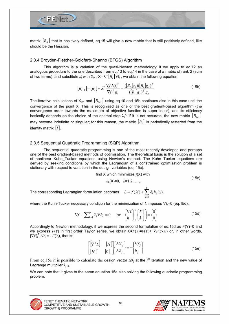
2.3.4 Broyden-Fletcher-Goldfarb-Shanno (BFGS) Algorithm This algorithm is a variation of the quasi-Newton methodology: if we apply to eq.12 an

analogous procedure to the one described from eq.13 to eq.14 in the case of a matrix of rank 2 (sum of two terms), and substitute di with Xi+1-Xi=λι∗ [ ]iB ∇fi , we obtain the following equation:

[ ] [ ] [ ] [ ][ ] i

Tii

Tiiii

iT

i

Tii

iii ggBgBgB

gfff

BB)(

))((*1 −

∇∇∇

+=+ λ

The iterative calculations of Xi+1 and [ ]1+iB using eq.10 and 15b continues also in this case until the convergence of the point X. This is recognized as one of the best gradient-based algorithm (the convergence order towards the maximum of objective function is super-linear), and its efficiency basically depends on the choice of the optimal step λι∗: if it is not accurate, the new matrix [ ]1+iB may become indefinite or singular; for this reason, the matrix [ ]iB is periodically restarted from the identity matrix [ ]I .

2.3.5 Sequential Quadratic Programming (SQP) Algorithm The sequential quadratic programming is one of the most recently developed and perhaps

one of the best gradient-based methods of optimisation. The theoretical basis is the solution of a set of nonlinear Kuhn_Tucker equations using Newton’s method. The Kuhn Tucker equations are derived by seeking conditions by which the Lagrangian of a constrained optimisation problem is stationary with respect to variation in the design variables (eq. 15c):

find X which minimizes f(X) with

hk(X)=0, k=1,2,….,p

The corresponding Lagrangian formulation becomes )()(1

xhXfL k

p

kk∑

=

+= λ ,

where the Kuhn-Tucker necessary condition for the minimization of L imposes ∇L=0 (eq.15d):

=

∇

=∇+∇ ∑ = 00

01 λλ

Xh

Lorhf k

p

k k

Accordingly to Newton methodology, if we express the second formulation of eq.15d as F(Y)=0 and we express F(Y) in first order Taylor series, we obtain 0=F(Y)=F(Yi)+ ∇F(Y-Yi) or, in other words, [∇F]jT ∆Yj = - F(Yi), that is:

[ ] [ ][ ] [ ]

∇

−=

∆

∆

∇

j

j

j

j

T hfX

H

HLλ0

2

From eq.15e it is possible to calculate the design vector ∆Xj at the jth iteration and the new value of Lagrange multiplier λj+1.

We can note that it gives to the same equation 15e also solving the following quadratic programming problem:

(15b)

(15c)

(15d)

(15e)



17

Find S= ∆X that minimize Q(S)= SHSSXf TT ][21)( +∇

subject to mjSXgXg Tjjj ,..,2,10)()( =≤∇+β

where [H] is given by [∇L2]: in fact, if we calculate the Lagrangian formulation L’ of Q(S) and we apply the Kuhn-Tucker necessary condition for the minimization of L’, we obtain the same equation 15e. This means that the original problem of eq.15c can be solved by a Newton methodology, and the [H] matrix of eq.15f can be updated in subsequent iterations like for BFGS methodology, so as to converge to the Hessian matrix [∇L2].

Once the search direction, S, is found by solving the equation 15f (applying Lagrangian formulation), the design vector is updated by Xj+1=Xj+α∗

S (with α∗ optimal step length), and the Hessian matrix [H]

is updated using a modified BFGS formula, such as:

[ ] [ ] [ ] [ ][ ] T

ii

T

iiTi

iTiii

ii SSSHSHSSH

HH γγ+−=+1

with ( ) ( )[ ] SHXLXL iii ])[1(1 θθγ −+∇−∇= +

2.4 Heuristics

2.4.1 Evolutionary algorithms Among the heuristics algorithms, the most common and used ones are the Evolutionary

Algorithms, and in particular the Genetic Algorithms (GA). They are the most robust, since they can be used for real and discrete variables, in highly or weakly non-linear problem types, for global search or refinement, and also for the resolution of multi-objective problems.

They are based on an analogy with the biological evolution, since the configurations defined by the different combination of variables, or individuals, improve their fitness generation after generation. Each individual is defined by the vector X=(x1,x2,…xn), n being the number of variables. There is an initial generation or set of m individuals (defined by a DOE strategy), and through different strategies of selection, like Roulette or Tournament, the individuals characterised by the best fitness (or value of the function) are chosen.

Fig.10 Selection by Roulette: each sector have a dimension proportional to each individual fitness

The selection by Roulette is represented in the figure 10 above: to each one of the m individuals is given a percentage range as large as the value of the fitness function. A random number between [0,1] is used to select one individual, and of course the probability that a good individual is chosen is greater. In the selection by Tournament, to each individual is compared each time the best individual of a sub-population of m/5 individual randomly chosen, m being the population size; the best of the two individual is chosen.

(15f)

(15g)



18

A last class of selection is the local one, for which to each individual is compared the best one of a subpopulation of 0.6 m individuals, not chosen randomly, but chosen as the closest individuals to the selected one; also in this case, the best of the two individuals is chosen. In the case of a multi-objective optimisation, an individual x* is chosen if it is non-dominated by the other ones. It means that, if fA and fB are the two functions to be minimised (see also fig.13), no solution X exists such that:

Once a proper number of individuals is selected, we obtain the m individuals of the next generation by the operations of cross-over and mutation. The cross-over is an operation that allows to obtain, starting from the old individuals (parents), new individuals (children), that however may conserve the best features of their parents. As first operation, the real value of each variable of the individual (xi) is to be converted in integer (Xi) by the following formula:

( )

−

−−

= 12intminmax

min nbitii xx

xxX

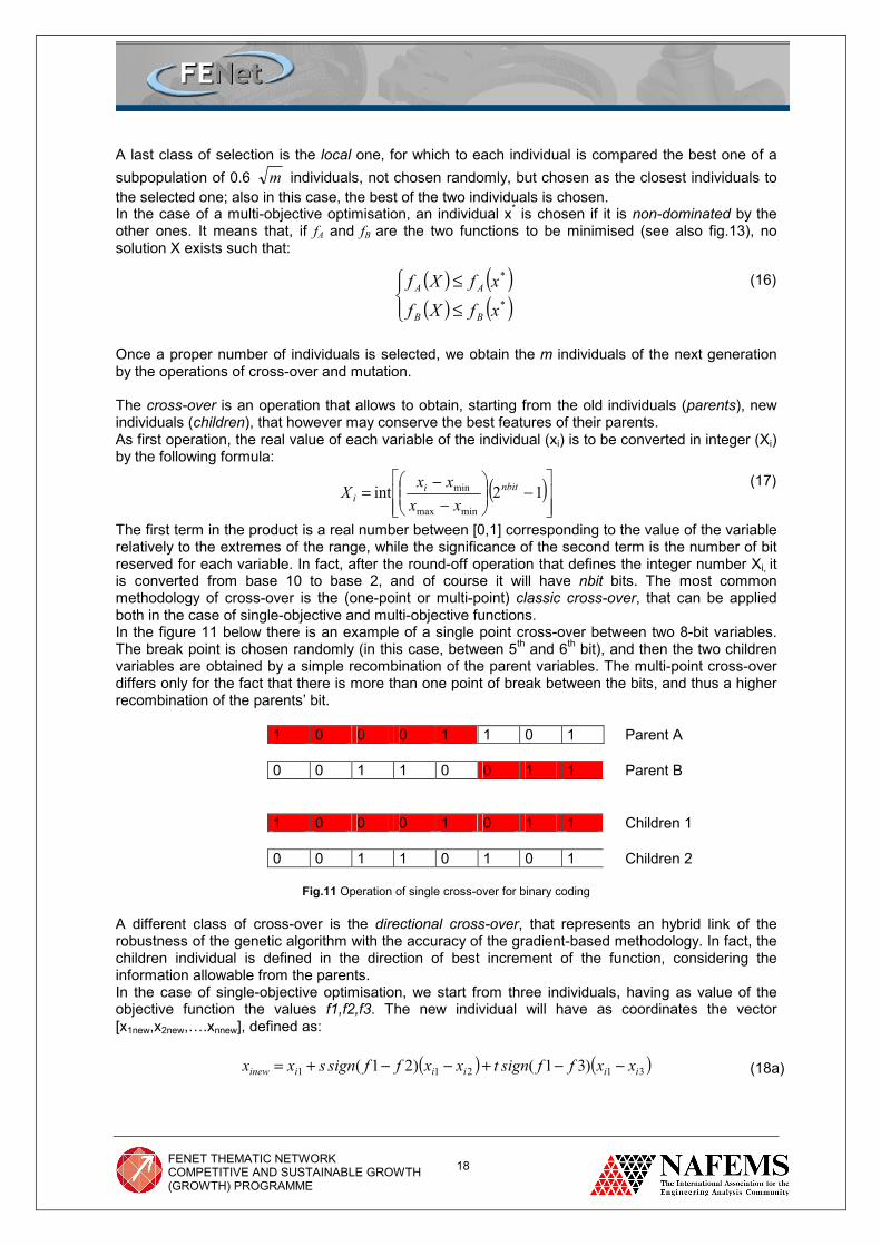
The first term in the product is a real number between [0,1] corresponding to the value of the variable relatively to the extremes of the range, while the significance of the second term is the number of bit reserved for each variable. In fact, after the round-off operation that defines the integer number Xi, it is converted from base 10 to base 2, and of course it will have nbit bits. The most common methodology of cross-over is the (one-point or multi-point) classic cross-over, that can be applied both in the case of single-objective and multi-objective functions. In the figure 11 below there is an example of a single point cross-over between two 8-bit variables. The break point is chosen randomly (in this case, between 5th and 6th bit), and then the two children variables are obtained by a simple recombination of the parent variables. The multi-point cross-over differs only for the fact that there is more than one point of break between the bits, and thus a higher recombination of the parents’ bit.

1 0 0 0 1 1 0 1 Parent A

0 0 1 1 0 0 1 1 Parent B

1 0 0 0 1 0 1 1 Children 1

0 0 1 1 0 1 0 1 Children 2

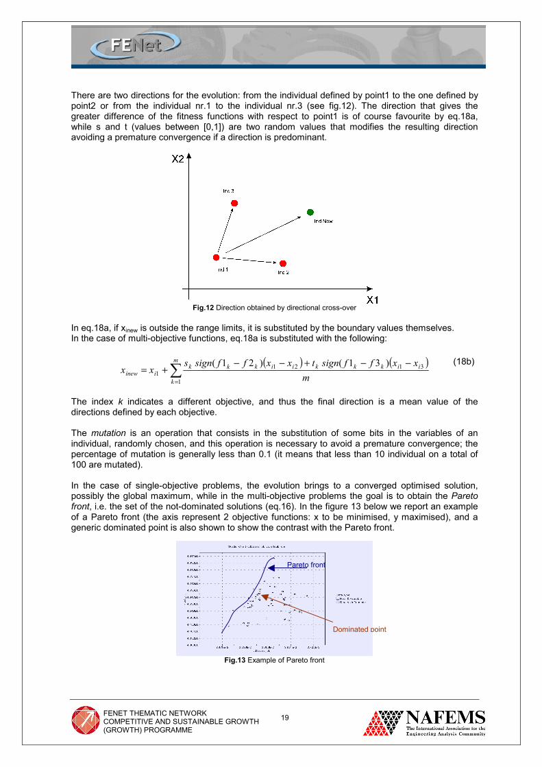
Fig.11 Operation of single cross-over for binary coding A different class of cross-over is the directional cross-over, that represents an hybrid link of the robustness of the genetic algorithm with the accuracy of the gradient-based methodology. In fact, the children individual is defined in the direction of best increment of the function, considering the information allowable from the parents. In the case of single-objective optimisation, we start from three individuals, having as value of the objective function the values f1,f2,f3. The new individual will have as coordinates the vector [x1new,x2new,….xnnew], defined as:

( ) ( )31211 )31()21( iiiiiinew xxffsigntxxffsignsxx −−+−−+=

( ) ( )( ) ( )

≤

≤*

*

xfXfxfXf

BB

AA (16)

(17)

(18a)



19

There are two directions for the evolution: from the individual defined by point1 to the one defined by point2 or from the individual nr.1 to the individual nr.3 (see fig.12). The direction that gives the greater difference of the fitness functions with respect to point1 is of course favourite by eq.18a, while s and t (values between [0,1]) are two random values that modifies the resulting direction avoiding a premature convergence if a direction is predominant.

Fig.12 Direction obtained by directional cross-over

In eq.18a, if xinew is outside the range limits, it is substituted by the boundary values themselves. In the case of multi-objective functions, eq.18a is substituted with the following:

( ) ( )∑=

−−+−−+=

m

k

iikkkiikkkiinew m

xxffsigntxxffsignsxx

1

31211

)31()21(

The index k indicates a different objective, and thus the final direction is a mean value of the directions defined by each objective. The mutation is an operation that consists in the substitution of some bits in the variables of an individual, randomly chosen, and this operation is necessary to avoid a premature convergence; the percentage of mutation is generally less than 0.1 (it means that less than 10 individual on a total of 100 are mutated). In the case of single-objective problems, the evolution brings to a converged optimised solution, possibly the global maximum, while in the multi-objective problems the goal is to obtain the Pareto front, i.e. the set of the not-dominated solutions (eq.16). In the figure 13 below we report an example of a Pareto front (the axis represent 2 objective functions: x to be minimised, y maximised), and a generic dominated point is also shown to show the contrast with the Pareto front.

Fig.13 Example of Pareto front

Dominated point

Pareto front

(18b)



20

2.4.2 Others (Simulated Annealing, Tabu Search, Genetic Programming, Game Theory, etc.)

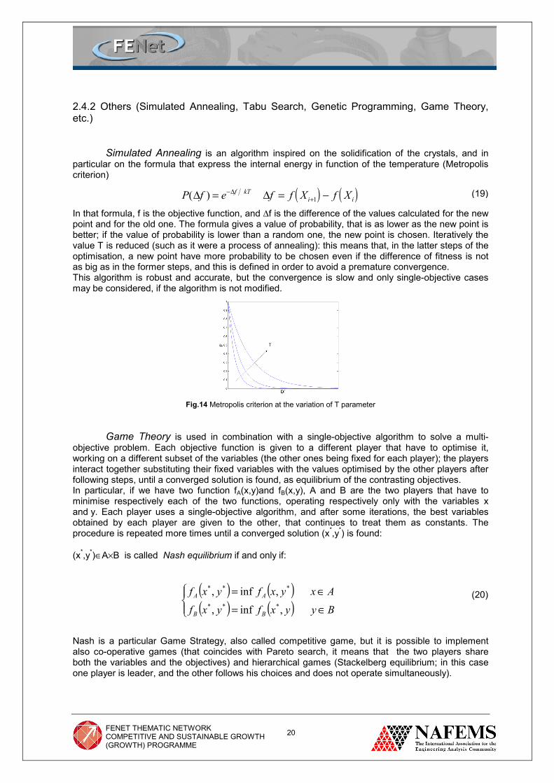
Simulated Annealing is an algorithm inspired on the solidification of the crystals, and in particular on the formula that express the internal energy in function of the temperature (Metropolis criterion)

In that formula, f is the objective function, and ∆f is the difference of the values calculated for the new point and for the old one. The formula gives a value of probability, that is as lower as the new point is better; if the value of probability is lower than a random one, the new point is chosen. Iteratively the value T is reduced (such as it were a process of annealing): this means that, in the latter steps of the optimisation, a new point have more probability to be chosen even if the difference of fitness is not as big as in the former steps, and this is defined in order to avoid a premature convergence. This algorithm is robust and accurate, but the convergence is slow and only single-objective cases may be considered, if the algorithm is not modified.

Fig.14 Metropolis criterion at the variation of T parameter

Game Theory is used in combination with a single-objective algorithm to solve a multi-objective problem. Each objective function is given to a different player that have to optimise it, working on a different subset of the variables (the other ones being fixed for each player); the players interact together substituting their fixed variables with the values optimised by the other players after following steps, until a converged solution is found, as equilibrium of the contrasting objectives. In particular, if we have two function fA(x,y)and fB(x,y), A and B are the two players that have to minimise respectively each of the two functions, operating respectively only with the variables x and y. Each player uses a single-objective algorithm, and after some iterations, the best variables obtained by each player are given to the other, that continues to treat them as constants. The procedure is repeated more times until a converged solution (x*,y*) is found: (x*,y*)∈A×B is called Nash equilibrium if and only if: Nash is a particular Game Strategy, also called competitive game, but it is possible to implement also co-operative games (that coincides with Pareto search, it means that the two players share both the variables and the objectives) and hierarchical games (Stackelberg equilibrium; in this case one player is leader, and the other follows his choices and does not operate simultaneously).

( ) ( )P f e f f X f Xf kTi i( )∆ ∆∆= = −−+1

(19)

( ) ( )( ) ( )

∈=

∈=

ByyxfyxfAxyxfyxf

BB

AA

,inf,,inf,***

***(20)



21

In any case, these methodologies represent a good alternative to the GA in the case of multi-objective optimisation. Even though they are not used to find a set of solutions, they could give a good solution as compromise of the different objectives, requiring a smaller number of computations. 3. A rough guide for methods to consider

APPLICABILITY TABLE: N=not applicable W = weakly applicable A = applicable R = recommended

A ROUGH GUIDE on methods to consider Problem type Gradient Simplex Heuristic Integer/Linear

prog Global

search Refinement Global

search Refinement Global search Refinement

Real variables A R A A R A N Discrete Variables N N W W R R R Mixed real/discrete N N W W R A N Weakly non linear A R R A A A W Highly non linear N, A* A W W R R N Few variables (<10) A A A R A A R Many variables (>10;<50)

W,A*,A** W,R*,R** A R R A W

Very many variables (>50)

W,A*,A** W,R*,R** A A R A N

* applicable on RSM produced after DOE **derivatives are available

Algorithms types Methods Types Comments References Linear/discrete programming

Only analytical S.Gass, Linear Programming, McGraw-Hill, New York, 1964

Simplex Single-objective Nelder, J:A., Mead, R., Computer Journal, 7, 308, 1965

Gradient BFGS Powell SPQ, Conjugate Gradient

Single-objective S.S.Rao, Engineering Optimisation, Theory and Practice, Wiley, 1996 R.L.Fox, Optimisation Methods for Engineering Design, Addison-Wesley, Reading, Mass., 1971

Heuristics Genetic Algorithms Evolution Strategy Simulated Annealing Tabu Search Evolutionary Structural Optimisation Genetic Programming Game Theory

Multi-objective Single-objective

Goldberg D.E., Genetic Algorithms in Search, Optimization & Machine Learning,. Addison-Wesley Publishing Company Inc.,Reading (Mass.),1989. P.vanLaarhoven ,E.Arts, Simulated Annealing:Theory and Applications, D.Reidel,Boston,1997 Nash, J.F Non-cooperative Games. Annals of Mathematics, 54, 289, 1951



22

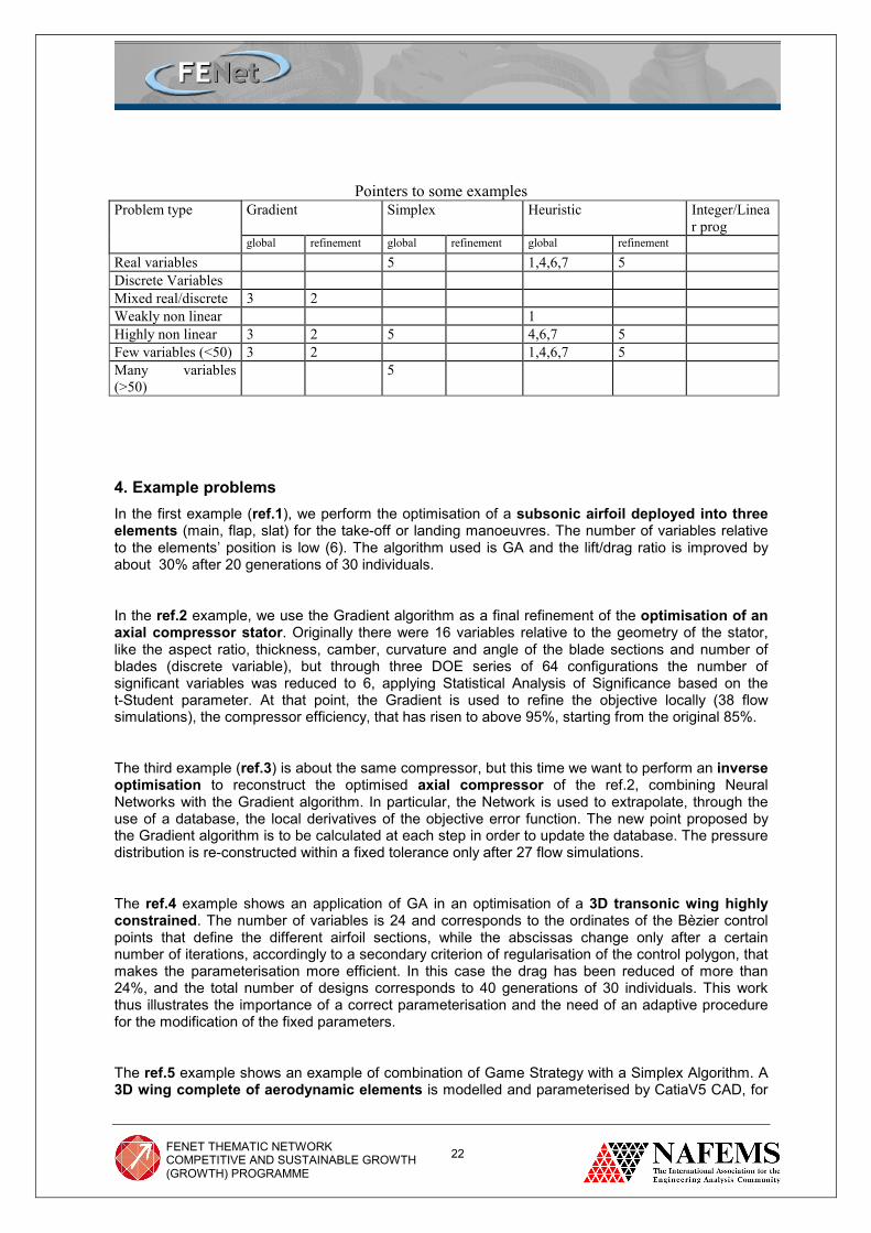
Pointers to some examples Problem type Gradient Simplex Heuristic Integer/Linea

r prog global refinement global refinement global refinement

Real variables 5 1,4,6,7 5 Discrete Variables Mixed real/discrete 3 2 Weakly non linear 1 Highly non linear 3 2 5 4,6,7 5 Few variables (<50) 3 2 1,4,6,7 5 Many variables (>50)

5

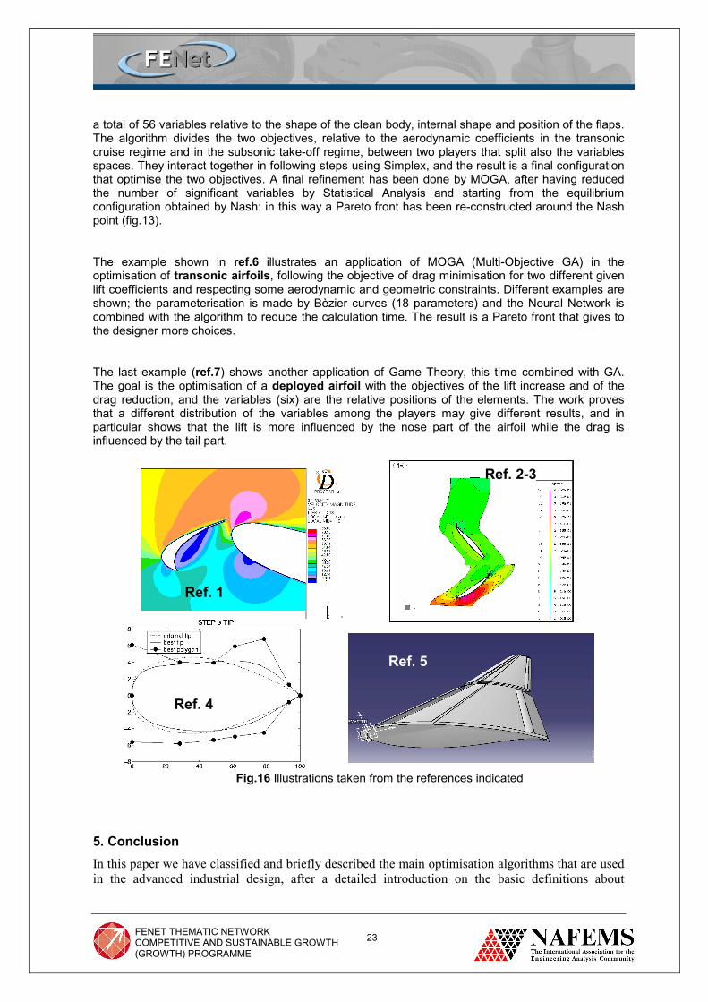
4. Example problems In the first example (ref.1), we perform the optimisation of a subsonic airfoil deployed into three elements (main, flap, slat) for the take-off or landing manoeuvres. The number of variables relative to the elements’ position is low (6). The algorithm used is GA and the lift/drag ratio is improved by about 30% after 20 generations of 30 individuals.

In the ref.2 example, we use the Gradient algorithm as a final refinement of the optimisation of an axial compressor stator. Originally there were 16 variables relative to the geometry of the stator, like the aspect ratio, thickness, camber, curvature and angle of the blade sections and number of blades (discrete variable), but through three DOE series of 64 configurations the number of significant variables was reduced to 6, applying Statistical Analysis of Significance based on the t-Student parameter. At that point, the Gradient is used to refine the objective locally (38 flow simulations), the compressor efficiency, that has risen to above 95%, starting from the original 85%.

The third example (ref.3) is about the same compressor, but this time we want to perform an inverse optimisation to reconstruct the optimised axial compressor of the ref.2, combining Neural Networks with the Gradient algorithm. In particular, the Network is used to extrapolate, through the use of a database, the local derivatives of the objective error function. The new point proposed by the Gradient algorithm is to be calculated at each step in order to update the database. The pressure distribution is re-constructed within a fixed tolerance only after 27 flow simulations.

The ref.4 example shows an application of GA in an optimisation of a 3D transonic wing highly constrained. The number of variables is 24 and corresponds to the ordinates of the Bèzier control points that define the different airfoil sections, while the abscissas change only after a certain number of iterations, accordingly to a secondary criterion of regularisation of the control polygon, that makes the parameterisation more efficient. In this case the drag has been reduced of more than 24%, and the total number of designs corresponds to 40 generations of 30 individuals. This work thus illustrates the importance of a correct parameterisation and the need of an adaptive procedure for the modification of the fixed parameters.

The ref.5 example shows an example of combination of Game Strategy with a Simplex Algorithm. A 3D wing complete of aerodynamic elements is modelled and parameterised by CatiaV5 CAD, for



23

a total of 56 variables relative to the shape of the clean body, internal shape and position of the flaps. The algorithm divides the two objectives, relative to the aerodynamic coefficients in the transonic cruise regime and in the subsonic take-off regime, between two players that split also the variables spaces. They interact together in following steps using Simplex, and the result is a final configuration that optimise the two objectives. A final refinement has been done by MOGA, after having reduced the number of significant variables by Statistical Analysis and starting from the equilibrium configuration obtained by Nash: in this way a Pareto front has been re-constructed around the Nash point (fig.13).

The example shown in ref.6 illustrates an application of MOGA (Multi-Objective GA) in the optimisation of transonic airfoils, following the objective of drag minimisation for two different given lift coefficients and respecting some aerodynamic and geometric constraints. Different examples are shown; the parameterisation is made by Bèzier curves (18 parameters) and the Neural Network is combined with the algorithm to reduce the calculation time. The result is a Pareto front that gives to the designer more choices.

The last example (ref.7) shows another application of Game Theory, this time combined with GA. The goal is the optimisation of a deployed airfoil with the objectives of the lift increase and of the drag reduction, and the variables (six) are the relative positions of the elements. The work proves that a different distribution of the variables among the players may give different results, and in particular shows that the lift is more influenced by the nose part of the airfoil while the drag is influenced by the tail part.

Fig.16 Illustrations taken from the references indicated

5. Conclusion In this paper we have classified and briefly described the main optimisation algorithms that are used in the advanced industrial design, after a detailed introduction on the basic definitions about

Ref. 1

Ref. 2-3

Ref. 4

Ref. 5



24

optimisation. We have collected some examples of application of these algorithms, especially in the aeronautic and turbo-machinery fields. As a matter of fact, the heuristic algorithms, and in particular the genetic algorithms, are widely applied for their robustness and efficiency, as they can equally be applied in problems involving a small or large number of variables, real or discrete variables, highly non-linear or linear problems, single-objective or multi-objective problems. The gradient based and simplex methods are often applied combined with RSM methodology and Doe techniques or in combination of Game Theory, in order to save calculation time in the first case or to transform multi-objective problems in competitive single-objective problems in the latter case. They are typically used, because of their accuracy, to refine locally a solution obtained by a heuristic algorithm.

Acknowledgements We’d like to express our gratitude to Peter Bartholomew for his suggestions and help in the correction of the paper, and to Nigel Knowles and all the other members of FENET project that participated at the PSO sessions with all their contributions.

References 1. A.Clarich, C.Poloni, Optimisation of a 3-element high lift configuration, Innovative Tools for

Scientific Computation in Aeronautical Engineering-Ed. by Periaux, Joly, Pironneau, Onate, pp. 262-271, CIMNE 2001, Barcelona

2. Alberto Clarich, Valentino Pediroda, Giovanni Mosetti, Carlo Poloni, Application of evolutive algorithms and statistical analysis in the numerical optimisation of an axial compressor, Acts of 9th International Symposium on Transport Phenomena and Dynamics of Rotating Machinery,Honolulu, Hawaii, February 10-14, 2002

3. A.Giassi, V.Pediroda, C.Poloni, A.Clarich, Three-dimensional inverse design of turbomachinery stage with neural-networks and direct flow solver, Inverse Problem in Engineering, Gordon and Breach Science Publishers, Vol.11, number 6, Taylor & Francis, pg. 457-470, December 2003

4. Alberto Clarich, Jean-Antoine Desideri, Self-adaptive parameterisation for aerodynamic optimum-shape design, Rapport de Recherche 4428, INRIA, March 2002

5. A.Clarich, J.Periaux,C.Poloni, Combining Game Strategies And Evolutionary Algorithms for CAD Parameterisation and multi-point Optimisation of Complex Aeronautic Systems, acts of EUROGEN 2003, Barcelona, September 2003

6. C.Poloni, A.Giurgevich, L.Onesti, V.Pediroda. Hybridization of a multi-objective genetic algorithm, a neural network and a classical optimizer for a complex design problem in fluid dynamic, pp. 403-420, Comput. Methods Appl. Mech.Engrg.186 , 2000.

7. J.F.Wang, J.Periaux, “Search Space Decomposition of Nash/Stackelberg Games using Genetic Algorithms for Multi-Point Design Optimization in Aerodynamics” from Domain Decomposition Methods in Science and Engineering, pp. 139-149, CIMNE 2002

[email protected]

[email protected]

[email protected]

[email protected]

[email protected]

[email protected]

[email protected]

Documents

The use of Optimisation algorithms in PSO - NAFEMS · The use of Optimisation algorithms in PSO Prof. Carlo Poloni, University of Trieste, Dr. Valentino Pediroda, University of Trieste,