The use of onboard UAV GNSS navigation data for area and

Acta Montanistica Slovaca, Volume 25 (2020),

The use of onboard UAV GNSS navigation data for area

and volume calculation Rudolf URBAN1*, Martin ŠTRONER

Authors’ affiliations and addresses: 1 Department of Special Geodesy, Faculty of Civil Engineering, Czech Technical University inPrague, Thákurova 7, 166 36 Prague 6, Czech Republic e-mail: [email protected]

2 Department of Special Geodesy, Faculty of Civil Engineering, Czech Technical University in Prague, Thákurova 7, 166 36 Prague 6, Czech Republic e-mail: [email protected]

3 Department of Automation and Production Systems, Faculty of Mechanical Engineering,University of Žilina, Univerzitná 8215/1, 010 26 Žilina, Slovakia e-mail: [email protected] *Correspondence:

Rudolf Urban, Department of Special GeodesyFaculty of Civil Engineering, Czech Technical University in Prague, Thákurova 7, 166 36 Prague 6, Czech Republic tel.: +42022435 4736 e-mail:[email protected] Funding information: Grant SGS20/052/OHK1/1T/11 funded by CTU Prague, Czech Republic. How to cite this article:

Urban, R., Štroner, M. and Kuric, I.(2020). The use of onboard UAV GNSS navigation data for area and volume calculation. Acta

Montanistica Slovaca, Volume 25 (3), 361- DOI: https://doi.org/10.46544/AMS.v25i3.9

© 2020 by the authors. Submitted for possible open access publication under the terms and conditions

of the Creative Commons Attribution (CC BY) license

(2020), 3; DOI: 10.46544/AMS.v25i3.9


and volume calculation

ŠTRONER2and Ivan KURIC3

Department of Special Geodesy, Faculty of Civil Engineering, Czech Technical University in Prague, Thákurova 7, 166 36 Prague 6, Czech

Department of Special Geodesy, Faculty of Civil Engineering, Czech Technical University in Prague, Thákurova 7, 166 36 Prague 6, Czech

Department of Automation and Production Faculty of Mechanical Engineering,

University of Žilina, Univerzitná 8215/1, 010 26

Department of Special Geodesy, Faculty of Civil Engineering, Czech Technical

Grant SGS20/052/OHK1/1T/11 funded by CTU

(2020). use of onboard UAV GNSS navigation data

-374

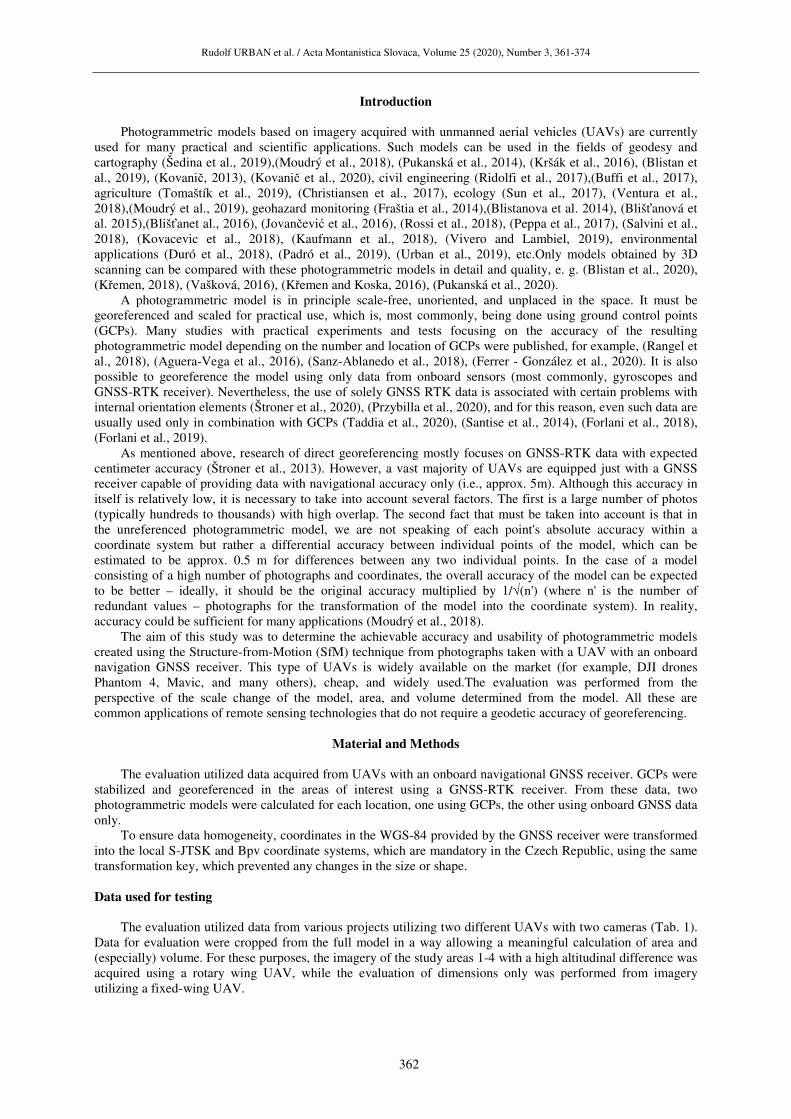
Abstract Photogrammetric models constructed from unmanned aerial vehicle (UAV) data are nowadays used for determining areas or volumes in many scientific and practical applications. The presented study discusses the possibility of direct georeferencing of photogrammetric models based on onboard navigational GNSS. It is widely expected that all UAV-derived data need to be georeferenced with a sub-decimeter accuracy. The aim of the work was to test whether it would not be enough to georeference photogrammetric models only using navigation GNSS. Imagery from several locations was used for the construction of photogrammetric models using GCPs or navigational GNSS only. All models were transformed into the same coordinate system using the same transformation key to facilitate comparisons. For the first comparisons, a 7-element transformation was performed to facilitate analysis of the systematic shift, rotation, and scale change between the models. It confirmed that the scale change of the photogrammetric model constructed using navigation GNSS data only from that constructed using GCPs was very small, with a maximum change of 2% (scale change of 0.98). The 7transformation also revealed that the models are mutually shifted and rotated. The tilts were below 2°, and the horizontal shifts are consistent with the (in)accuracy of the navigational GNSS (the highest deviation was 3.7m). The data were also transformed using a 4-element transformation (shifted and rotated along the Zenable an analysis of the change of the shape. Subsequently, areas and volumes of both point clouds were calculated; the differences in volumes were below 10%, differences in areas even below 4%. For analysis of local deformations on an extensive site, an airfield area was used. The analysis of distances measured on an orthophotomosaic of a relatively large area (9.5 km2) revealed a mean absolute deviation between the GNSS and GCP data, which is a surprisingly good result. This method is suitable for identifying potential local deformations that can occur in photogrammetric models in the spaces between GCPs. The reported experiments demonstrate that the calculations of volumes and areas using only onboard UAV GNSS navigation data can be sufficient for many applications.

Keywords

UAV, photogrammetry, GCPs, navigation GNSS, precision, accuracy, usability;


of the Creative Commons Attribution (CC BY) license (http://creativecommons.org/licenses/by/4.0/).


Photogrammetric models constructed from unmanned aerial vehicle (UAV) data are nowadays used for determining areas or volumes in many scientific and practical applications. The presented study discusses the possibility of direct georeferencing of

metric models based on onboard navigational GNSS. It is derived data need to be

decimeter accuracy. The aim of the work was to test whether it would not be enough to georeference

only using navigation GNSS. Imagery from several locations was used for the construction of photogrammetric models using GCPs or navigational GNSS only. All models were transformed into the same coordinate system using

tate comparisons. For the first element transformation was performed to facilitate

analysis of the systematic shift, rotation, and scale change between the models. It confirmed that the scale change of the

using navigation GNSS data only from that constructed using GCPs was very small, with a maximum change of 2% (scale change of 0.98). The 7-element transformation also revealed that the models are mutually shifted

the horizontal shifts are consistent with the (in)accuracy of the navigational GNSS (the highest deviation was 3.7m). The data were also transformed using

element transformation (shifted and rotated along the Z-axis) to of the shape. Subsequently, areas

and volumes of both point clouds were calculated; the differences in volumes were below 10%, differences in areas even below 4%. For analysis of local deformations on an extensive site, an airfield area

ysis of distances measured on an orthophotomosaic of a relatively large area (9.5 km2) revealed a mean absolute deviation between the GNSS and GCP data, which is a surprisingly good result. This method is suitable for identifying

ns that can occur in photogrammetric models in the spaces between GCPs. The reported experiments demonstrate that the calculations of volumes and areas using only onboard UAV GNSS navigation data can be sufficient for many

ogrammetry, GCPs, navigation GNSS, precision,


(http://creativecommons.org/licenses/by/4.0/).

Rudolf URBAN et al. / Acta Montanistica Slovaca, Volume 25 (2020), Number 3, 361-374

362

Introduction

Photogrammetric models based on imagery acquired with unmanned aerial vehicles (UAVs) are currently

used for many practical and scientific applications. Such models can be used in the fields of geodesy and cartography (Šedina et al., 2019),(Moudrý et al., 2018), (Pukanská et al., 2014), (Kršák et al., 2016), (Blistan et al., 2019), (Kovanič, 2013), (Kovanič et al., 2020), civil engineering (Ridolfi et al., 2017),(Buffi et al., 2017), agriculture (Tomaštík et al., 2019), (Christiansen et al., 2017), ecology (Sun et al., 2017), (Ventura et al., 2018),(Moudrý et al., 2019), geohazard monitoring (Fraštia et al., 2014),(Blistanova et al. 2014), (Blišťanová et al. 2015),(Blišťanet al., 2016), (Jovančević et al., 2016), (Rossi et al., 2018), (Peppa et al., 2017), (Salvini et al., 2018), (Kovacevic et al., 2018), (Kaufmann et al., 2018), (Vivero and Lambiel, 2019), environmental applications (Duró et al., 2018), (Padró et al., 2019), (Urban et al., 2019), etc.Only models obtained by 3D scanning can be compared with these photogrammetric models in detail and quality, e. g. (Blistan et al., 2020), (Křemen, 2018), (Vašková, 2016), (Křemen and Koska, 2016), (Pukanská et al., 2020).

A photogrammetric model is in principle scale-free, unoriented, and unplaced in the space. It must be georeferenced and scaled for practical use, which is, most commonly, being done using ground control points (GCPs). Many studies with practical experiments and tests focusing on the accuracy of the resulting photogrammetric model depending on the number and location of GCPs were published, for example, (Rangel et al., 2018), (Aguera-Vega et al., 2016), (Sanz-Ablanedo et al., 2018), (Ferrer - González et al., 2020). It is also possible to georeference the model using only data from onboard sensors (most commonly, gyroscopes and GNSS-RTK receiver). Nevertheless, the use of solely GNSS RTK data is associated with certain problems with internal orientation elements (Štroner et al., 2020), (Przybilla et al., 2020), and for this reason, even such data are usually used only in combination with GCPs (Taddia et al., 2020), (Santise et al., 2014), (Forlani et al., 2018), (Forlani et al., 2019).

As mentioned above, research of direct georeferencing mostly focuses on GNSS-RTK data with expected centimeter accuracy (Štroner et al., 2013). However, a vast majority of UAVs are equipped just with a GNSS receiver capable of providing data with navigational accuracy only (i.e., approx. 5m). Although this accuracy in itself is relatively low, it is necessary to take into account several factors. The first is a large number of photos (typically hundreds to thousands) with high overlap. The second fact that must be taken into account is that in the unreferenced photogrammetric model, we are not speaking of each point's absolute accuracy within a coordinate system but rather a differential accuracy between individual points of the model, which can be estimated to be approx. 0.5 m for differences between any two individual points. In the case of a model consisting of a high number of photographs and coordinates, the overall accuracy of the model can be expected to be better – ideally, it should be the original accuracy multiplied by 1/√(n') (where n' is the number of redundant values – photographs for the transformation of the model into the coordinate system). In reality, accuracy could be sufficient for many applications (Moudrý et al., 2018).

The aim of this study was to determine the achievable accuracy and usability of photogrammetric models created using the Structure-from-Motion (SfM) technique from photographs taken with a UAV with an onboard navigation GNSS receiver. This type of UAVs is widely available on the market (for example, DJI drones Phantom 4, Mavic, and many others), cheap, and widely used.The evaluation was performed from the perspective of the scale change of the model, area, and volume determined from the model. All these are common applications of remote sensing technologies that do not require a geodetic accuracy of georeferencing.

Material and Methods

The evaluation utilized data acquired from UAVs with an onboard navigational GNSS receiver. GCPs were

stabilized and georeferenced in the areas of interest using a GNSS-RTK receiver. From these data, two photogrammetric models were calculated for each location, one using GCPs, the other using onboard GNSS data only.

To ensure data homogeneity, coordinates in the WGS-84 provided by the GNSS receiver were transformed into the local S-JTSK and Bpv coordinate systems, which are mandatory in the Czech Republic, using the same transformation key, which prevented any changes in the size or shape.

Data used for testing

The evaluation utilized data from various projects utilizing two different UAVs with two cameras (Tab. 1).

Data for evaluation were cropped from the full model in a way allowing a meaningful calculation of area and (especially) volume. For these purposes, the imagery of the study areas 1-4 with a high altitudinal difference was acquired using a rotary wing UAV, while the evaluation of dimensions only was performed from imagery utilizing a fixed-wing UAV.


363

Tab. 1 Used UAVs, cameras, and overlap

Study area UAV Camera Camera Resolution Front and side overlap

1 - 4 DJI Phantom 4 Pro FC6310 5472 x 3648 60 %

5 SenseFlyeBee S.O.D.A 5472 x 3648 60 %

In all locations, GCPs were placed (in figures marked by red dots) and georeferenced using GNSS RTK

(Trimble Geo XR) with the accuracy of GCP 0.03 m. Photogrammetric models were calculated in the Agisoft Metashape v. 1.6.3.

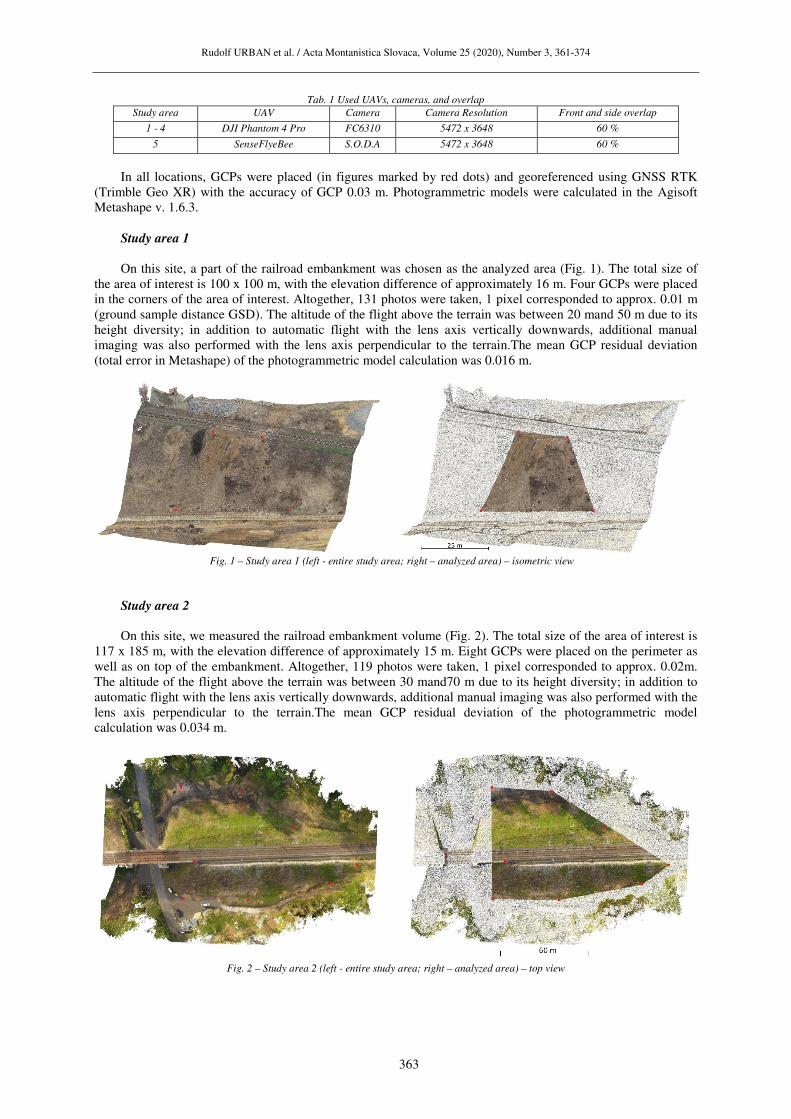
Study area 1 On this site, a part of the railroad embankment was chosen as the analyzed area (Fig. 1). The total size of

the area of interest is 100 x 100 m, with the elevation difference of approximately 16 m. Four GCPs were placed in the corners of the area of interest. Altogether, 131 photos were taken, 1 pixel corresponded to approx. 0.01 m (ground sample distance GSD). The altitude of the flight above the terrain was between 20 mand 50 m due to its height diversity; in addition to automatic flight with the lens axis vertically downwards, additional manual imaging was also performed with the lens axis perpendicular to the terrain.The mean GCP residual deviation (total error in Metashape) of the photogrammetric model calculation was 0.016 m.

Fig. 1 – Study area 1 (left - entire study area; right – analyzed area) – isometric view

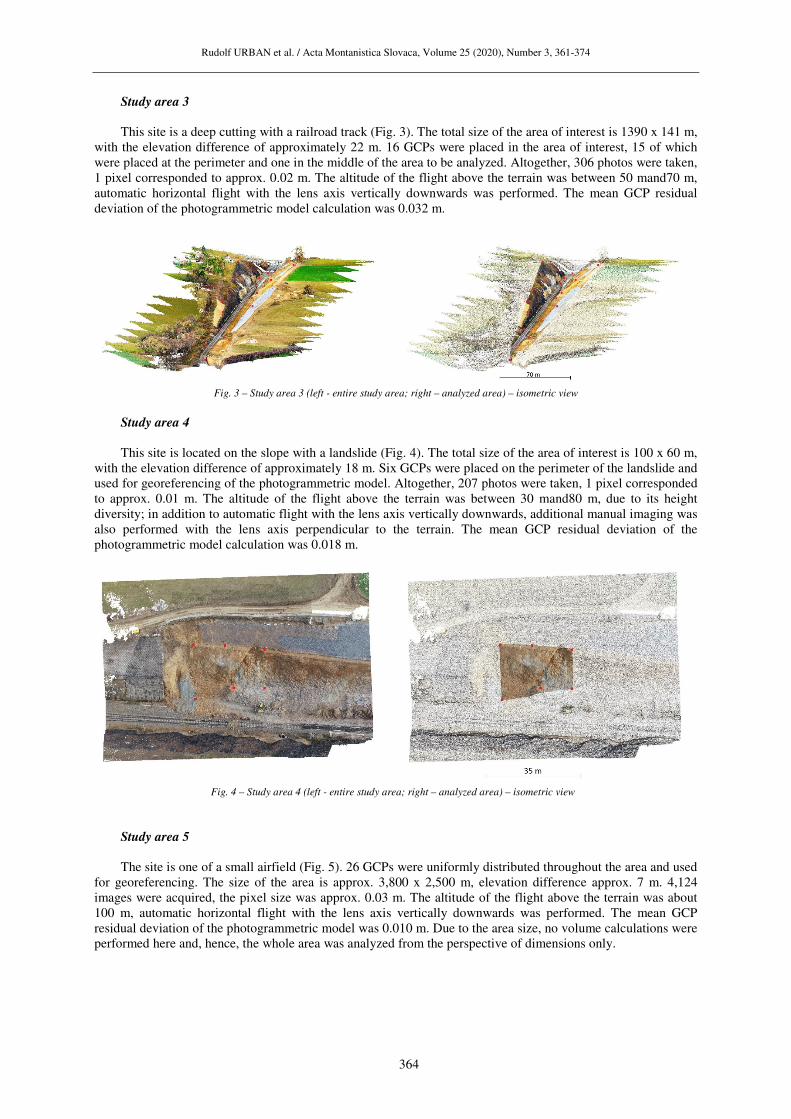
Study area 2 On this site, we measured the railroad embankment volume (Fig. 2). The total size of the area of interest is

117 x 185 m, with the elevation difference of approximately 15 m. Eight GCPs were placed on the perimeter as well as on top of the embankment. Altogether, 119 photos were taken, 1 pixel corresponded to approx. 0.02m. The altitude of the flight above the terrain was between 30 mand70 m due to its height diversity; in addition to automatic flight with the lens axis vertically downwards, additional manual imaging was also performed with the lens axis perpendicular to the terrain.The mean GCP residual deviation of the photogrammetric model calculation was 0.034 m.

Fig. 2 – Study area 2 (left - entire study area; right – analyzed area) – top view


364

Study area 3 This site is a deep cutting with a railroad track (Fig. 3). The total size of the area of interest is 1390 x 141 m,

with the elevation difference of approximately 22 m. 16 GCPs were placed in the area of interest, 15 of which were placed at the perimeter and one in the middle of the area to be analyzed. Altogether, 306 photos were taken, 1 pixel corresponded to approx. 0.02 m. The altitude of the flight above the terrain was between 50 mand70 m, automatic horizontal flight with the lens axis vertically downwards was performed. The mean GCP residual deviation of the photogrammetric model calculation was 0.032 m.


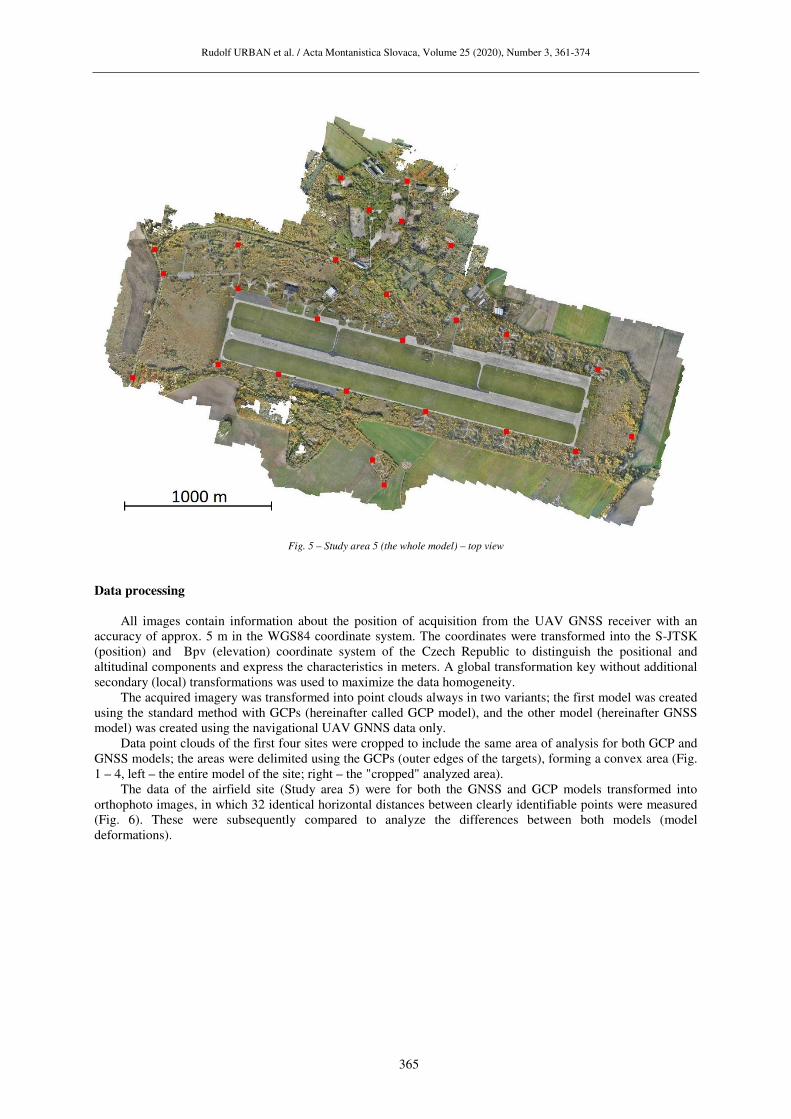
Study area 4 This site is located on the slope with a landslide (Fig. 4). The total size of the area of interest is 100 x 60 m,

with the elevation difference of approximately 18 m. Six GCPs were placed on the perimeter of the landslide and used for georeferencing of the photogrammetric model. Altogether, 207 photos were taken, 1 pixel corresponded to approx. 0.01 m. The altitude of the flight above the terrain was between 30 mand80 m, due to its height diversity; in addition to automatic flight with the lens axis vertically downwards, additional manual imaging was also performed with the lens axis perpendicular to the terrain. The mean GCP residual deviation of the photogrammetric model calculation was 0.018 m.


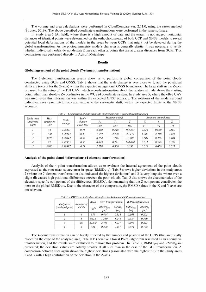
Study area 5

The site is one of a small airfield (Fig. 5). 26 GCPs were uniformly distributed throughout the area and used for georeferencing. The size of the area is approx. 3,800 x 2,500 m, elevation difference approx. 7 m. 4,124 images were acquired, the pixel size was approx. 0.03 m. The altitude of the flight above the terrain was about 100 m, automatic horizontal flight with the lens axis vertically downwards was performed. The mean GCP residual deviation of the photogrammetric model was 0.010 m. Due to the area size, no volume calculations were performed here and, hence, the whole area was analyzed from the perspective of dimensions only.


365

Fig. 5 – Study area 5 (the whole model) – top view

Data processing

All images contain information about the position of acquisition from the UAV GNSS receiver with an accuracy of approx. 5 m in the WGS84 coordinate system. The coordinates were transformed into the S-JTSK (position) and Bpv (elevation) coordinate system of the Czech Republic to distinguish the positional and altitudinal components and express the characteristics in meters. A global transformation key without additional secondary (local) transformations was used to maximize the data homogeneity.

The acquired imagery was transformed into point clouds always in two variants; the first model was created using the standard method with GCPs (hereinafter called GCP model), and the other model (hereinafter GNSS model) was created using the navigational UAV GNNS data only.

Data point clouds of the first four sites were cropped to include the same area of analysis for both GCP and GNSS models; the areas were delimited using the GCPs (outer edges of the targets), forming a convex area (Fig. 1 – 4, left – the entire model of the site; right – the "cropped" analyzed area).

The data of the airfield site (Study area 5) were for both the GNSS and GCP models transformed into orthophoto images, in which 32 identical horizontal distances between clearly identifiable points were measured (Fig. 6). These were subsequently compared to analyze the differences between both models (model deformations).


366

Fig. 6 – The measured distances in the Study area 5 (measured distances marked by yellow lines)

Accuracy assessment

Each tested site was represented by point clouds calculated with GCPs (GCP model) and with GNSS data

only (GNSS model) in the same coordinate system (position in S-JTSK and elevation in Bpv). For analysis of the resulting point clouds, a 7-element spatial transformation was calculated to define the mutual rotation in the Rotation matrix R (three angles of rotation around the three coordinate axes α, β, γ), scale change (coefficient m), and a systematic shift of the coordinates (coefficients TX, TY, TZ). Mathematically, the transformation can, therefore, be written as:

�� = � ∙ �, , �� ∙ �� + �� , (1)

where the X, Y, Z are the coordinates of the GCPs in the point cloud constructed with GCPs and x,y,z are coordinates of GCPs (or, in this case, checkpoints) calculated from the GNSS model.

The resulting coefficients show the global mutual rotation of both point clouds, their global systematic shifts, and the scale change. These data were used for the assessment of the overall agreement between the models.

In addition, to be able to evaluate other deformations of the photogrammetric model and resulting practical usability of the GNSS-derived model, a 4-element transformation was performed, in which only the rotation around the Z-axis and systematic shifts in three axes (TX, TY, TZ coefficients) were calculated. The models' scales and tilt were not changed to fit each other, which allowed us to analyze the scale change and differences between results calculated from these two models. RMSD (root mean square difference) in individual axes was chosen as the measure of the (dis)agreement between the models. An additional 4-element transformation was also performed using the iterative closest point (ICP) algorithm applied to the full point clouds. Hereinafter, we will use the terms ICP transformation and GCP transformation to describe these two methods.

Subsequently, the areas and volumes of the Study areas 1-4 were compared. Volumes were calculated relative to a flat, strictly horizontal plane intersecting the lowest point of the analyzed area. The four-element transformation was used to analyze local deformations of the models on the volume calculated from the point clouds. The two models of each site were intersected, and the volumes of added and removed material were determined.


367

The volume and area calculations were performed in CloudCompare ver. 2.11.0, using the raster method (Štroner, 2019),. The above described coordinate transformations were performed in the same software.

In Study area 5 (Airfield), where there is a high amount of data and the terrain is not rugged, horizontal distances of identical points were determined on the orthophotomosaic of both GCP and GNSS models to reveal potential local deformations of the models in the areas between GCPs that might not be detected during the global transformation. As the photogrammetric model's character is generally elastic, it was necessary to verify whether individual models do not deviate from each other at points that are at greater distances from GCPs. This comparison was performed directly in Agisoft Metashape.

Results

Global agreement of the point clouds (7-element transformation)

The 7-element transformation results allow us to perform a global comparison of the point clouds constructed using GCPs and GNSS. Tab. 2 shows that the scale change is very close to 1, and the positional shifts are (except for the Z-axis) within the expected navigational GNSS boundaries. The large shift in the Z-axis is caused by the setup of the DJI UAV, which records information about the relative altitude above the starting point rather than absolute Z-coordinates in the WGS84 coordinate system. In Study area 5, where the eBee UAV was used, even this information was within the expected GNSS accuracy. The rotations of the models around individual axes (yaw, pitch, roll) are, similar to the systematic shift, within the expected limits of the GNSS accuracy.

Tab. 2 – Comparison of individual site modelsusingthe 7-element transformation

Study area

(analyzed

part)

Max.

dimension

[m]

Scale

change

Scale

change

effect [m]

Systematic shift Rotation around axes

Tx Ty Tz X Y Z

[m] [m] [m] [°] [°] [°]

1 44 0.98291 0.75 0.690 0.348 184.337 0.332 0.630 0.569

2 120 1.00244 0.30 1.509 2.738 22.935 1.387 2.318 0.421

3 1210 1.00043 0.52 0.154 1.716 18.707 0.609 0.366 0.704

4 27 0.97955 0.55 0.019 0.271 114.098 0.011 0.596 0.390

5 3800 0.99997 0.11 2.178 0.960 0.398 0.038 0.050 0.021

Analysis of the point cloud deformations (4-element transformation)

Analysis of the 4-point transformation allows us to evaluate the internal agreement of the point clouds

expressed as the root mean square error in space (RMSDXYZ). Tab. 3 shows higher deviations in the study areas 2 (where the 7-element transformation also indicated the highest deviations) and 3 (a very long site where even a slight tilt causes high positional differences between the point clouds. Tab. 3 also shows the characteristics of the elevation-specific component of the differences (RMSDZ), demonstrating that the Z component contributes the most to the global RMSDXYZ. Due to the character of the comparison, the RMSD values in the X and Y axes are not relevant.

Tab. 3 – RMSDs at individual sites after the 4-element GCP transformation

Study area

(analyzed part)

Number of

GCPs

Area GCP transformation ICP transformation

[m2] RMSDXYZ

[m]

RMSDZ

[m]

RMSDXYZ

[m]

RMSDZ

[m]

1 4 875 0.464 0.338 0.168 0.203

2 8 6418 1.359 1.244 0.587 0.569

3 16 37278 2.485 1.277 0.993 0.893

4 6 421 0.328 0.457 0.074 0.128

The 4-point transformation can be highly affected by the number and position of the GCPs (that are usually placed on the edge of the analyzed area). The ICP (Iterative Closest Point) algorithm was used as an alternative transformation, and the results were evaluated to remove this problem. In Table 3, RMSDXYZ and RMSDZ are presented; the deviation values are notably smaller at all sites than in the case of the GCP transformation. A comparison between sites again shows the highest deviations (associated with the highest tilt) in the Study areas 2 and 3 with a high contribution of the deviation in the Z-axis.


368

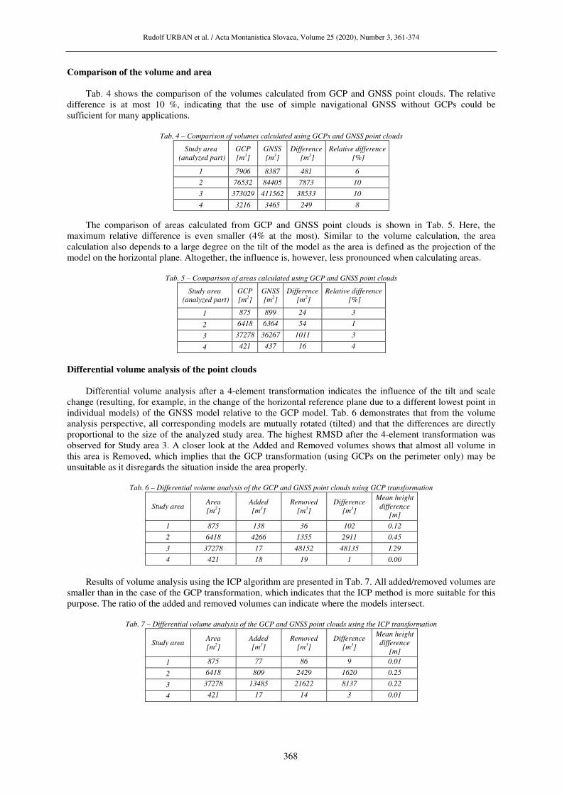
Comparison of the volume and area

Tab. 4 shows the comparison of the volumes calculated from GCP and GNSS point clouds. The relative

difference is at most 10 %, indicating that the use of simple navigational GNSS without GCPs could be sufficient for many applications.

Tab. 4 – Comparison of volumes calculated using GCPs and GNSS point clouds

Study area

(analyzed part)

GCP

[m3]

GNSS

[m3]

Difference

[m3]

Relative difference

[%]

1 7906 8387 481 6

2 76532 84405 7873 10

3 373029 411562 38533 10

4 3216 3465 249 8

The comparison of areas calculated from GCP and GNSS point clouds is shown in Tab. 5. Here, the maximum relative difference is even smaller (4% at the most). Similar to the volume calculation, the area calculation also depends to a large degree on the tilt of the model as the area is defined as the projection of the model on the horizontal plane. Altogether, the influence is, however, less pronounced when calculating areas.

Tab. 5 – Comparison of areas calculated using GCP and GNSS point clouds

Study area

(analyzed part)

GCP

[m2]

GNSS

[m2]

Difference

[m2]

Relative difference

[%]

1 875 899 24 3

2 6418 6364 54 1

3 37278 36267 1011 3

4 421 437 16 4

Differential volume analysis of the point clouds

Differential volume analysis after a 4-element transformation indicates the influence of the tilt and scale change (resulting, for example, in the change of the horizontal reference plane due to a different lowest point in individual models) of the GNSS model relative to the GCP model. Tab. 6 demonstrates that from the volume analysis perspective, all corresponding models are mutually rotated (tilted) and that the differences are directly proportional to the size of the analyzed study area. The highest RMSD after the 4-element transformation was observed for Study area 3. A closer look at the Added and Removed volumes shows that almost all volume in this area is Removed, which implies that the GCP transformation (using GCPs on the perimeter only) may be unsuitable as it disregards the situation inside the area properly.

Tab. 6 – Differential volume analysis of the GCP and GNSS point clouds using GCP transformation

Study area Area

[m2]

Added

[m3]

Removed

[m3]

Difference

[m3]

Mean height

difference

[m]

1 875 138 36 102 0.12

2 6418 4266 1355 2911 0.45

3 37278 17 48152 48135 I.29

4 421 18 19 1 0.00

Results of volume analysis using the ICP algorithm are presented in Tab. 7. All added/removed volumes are

smaller than in the case of the GCP transformation, which indicates that the ICP method is more suitable for this purpose. The ratio of the added and removed volumes can indicate where the models intersect.

Tab. 7 – Differential volume analysis of the GCP and GNSS point clouds using the ICP transformation

Study area Area

[m2]

Added

[m3]

Removed

[m3]

Difference

[m3]

Mean height

difference

[m]

1 875 77 86 9 0.01

2 6418 809 2429 1620 0.25

3 37278 13485 21622 8137 0.22

4 421 17 14 3 0.01


369

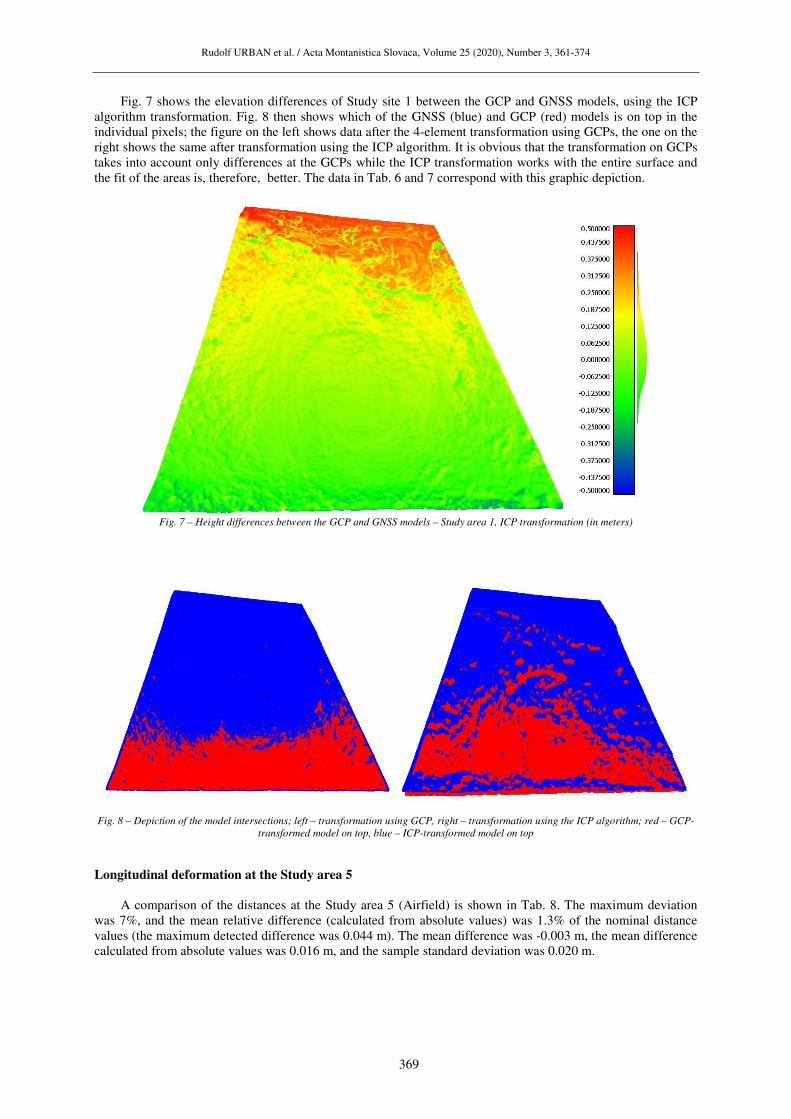
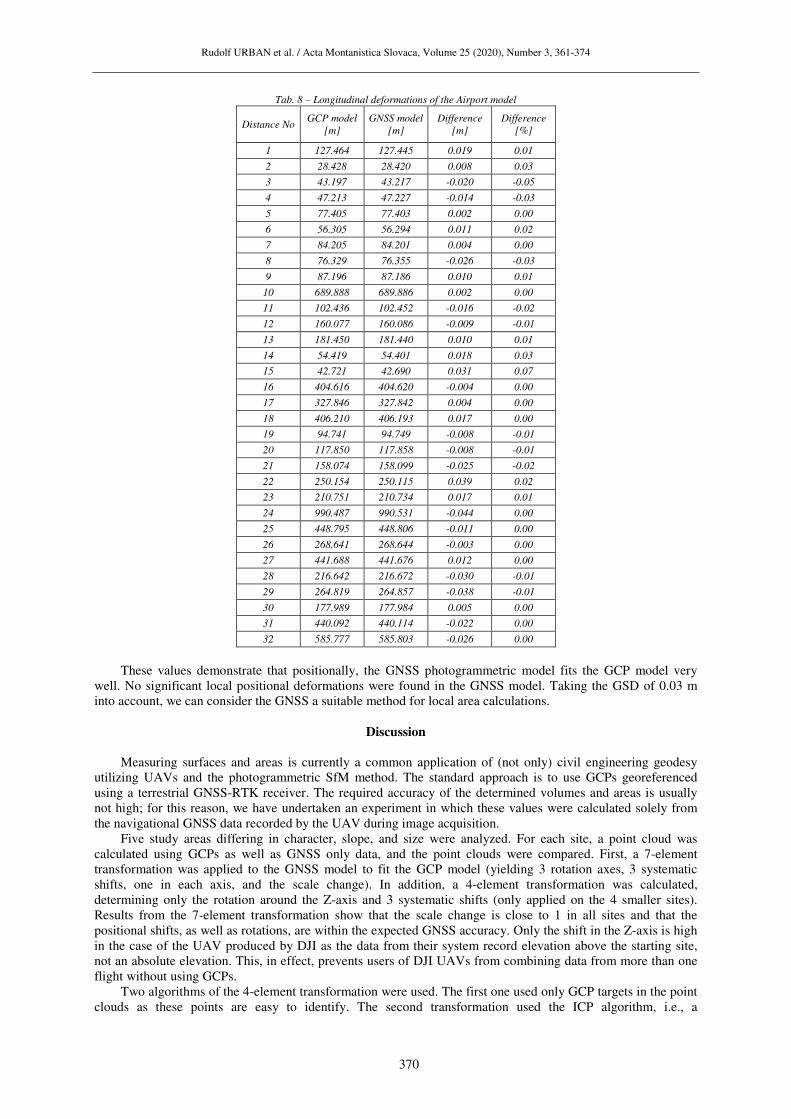
Fig. 7 shows the elevation differences of Study site 1 between the GCP and GNSS models, using the ICP algorithm transformation. Fig. 8 then shows which of the GNSS (blue) and GCP (red) models is on top in the individual pixels; the figure on the left shows data after the 4-element transformation using GCPs, the one on the right shows the same after transformation using the ICP algorithm. It is obvious that the transformation on GCPs takes into account only differences at the GCPs while the ICP transformation works with the entire surface and the fit of the areas is, therefore, better. The data in Tab. 6 and 7 correspond with this graphic depiction.

Fig. 7 – Height differences between the GCP and GNSS models – Study area 1, ICP transformation (in meters)

Fig. 8 – Depiction of the model intersections; left – transformation using GCP, right – transformation using the ICP algorithm; red – GCP-

transformed model on top, blue – ICP-transformed model on top

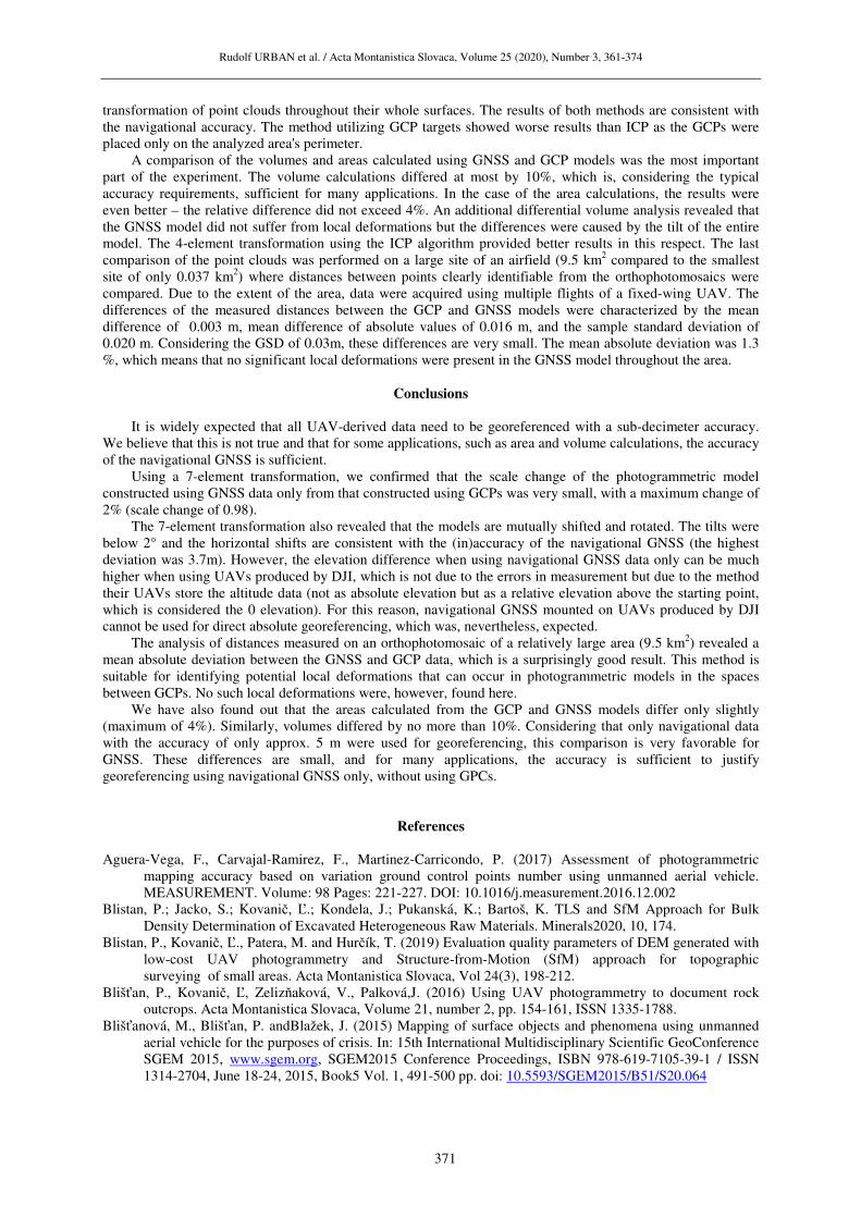
Longitudinal deformation at the Study area 5

A comparison of the distances at the Study area 5 (Airfield) is shown in Tab. 8. The maximum deviation was 7%, and the mean relative difference (calculated from absolute values) was 1.3% of the nominal distance values (the maximum detected difference was 0.044 m). The mean difference was -0.003 m, the mean difference calculated from absolute values was 0.016 m, and the sample standard deviation was 0.020 m.


370

Tab. 8 – Longitudinal deformations of the Airport model

Distance No GCP model

[m]

GNSS model

[m]

Difference

[m]

Difference

[%]

1 127.464 127.445 0.019 0.01

2 28.428 28.420 0.008 0.03

3 43.197 43.217 -0.020 -0.05

4 47.213 47.227 -0.014 -0.03

5 77.405 77.403 0.002 0.00

6 56.305 56.294 0.011 0.02

7 84.205 84.201 0.004 0.00

8 76.329 76.355 -0.026 -0.03

9 87.196 87.186 0.010 0.01

10 689.888 689.886 0.002 0.00

11 102.436 102.452 -0.016 -0.02

12 160.077 160.086 -0.009 -0.01

13 181.450 181.440 0.010 0.01

14 54.419 54.401 0.018 0.03

15 42.721 42.690 0.031 0.07

16 404.616 404.620 -0.004 0.00

17 327.846 327.842 0.004 0.00

18 406.210 406.193 0.017 0.00

19 94.741 94.749 -0.008 -0.01

20 117.850 117.858 -0.008 -0.01

21 158.074 158.099 -0.025 -0.02

22 250.154 250.115 0.039 0.02

23 210.751 210.734 0.017 0.01

24 990.487 990.531 -0.044 0.00

25 448.795 448.806 -0.011 0.00

26 268.641 268.644 -0.003 0.00

27 441.688 441.676 0.012 0.00

28 216.642 216.672 -0.030 -0.01

29 264.819 264.857 -0.038 -0.01

30 177.989 177.984 0.005 0.00

31 440.092 440.114 -0.022 0.00

32 585.777 585.803 -0.026 0.00

These values demonstrate that positionally, the GNSS photogrammetric model fits the GCP model very well. No significant local positional deformations were found in the GNSS model. Taking the GSD of 0.03 m into account, we can consider the GNSS a suitable method for local area calculations.

Discussion

Measuring surfaces and areas is currently a common application of (not only) civil engineering geodesy

utilizing UAVs and the photogrammetric SfM method. The standard approach is to use GCPs georeferenced using a terrestrial GNSS-RTK receiver. The required accuracy of the determined volumes and areas is usually not high; for this reason, we have undertaken an experiment in which these values were calculated solely from the navigational GNSS data recorded by the UAV during image acquisition.

Five study areas differing in character, slope, and size were analyzed. For each site, a point cloud was calculated using GCPs as well as GNSS only data, and the point clouds were compared. First, a 7-element transformation was applied to the GNSS model to fit the GCP model (yielding 3 rotation axes, 3 systematic shifts, one in each axis, and the scale change). In addition, a 4-element transformation was calculated, determining only the rotation around the Z-axis and 3 systematic shifts (only applied on the 4 smaller sites). Results from the 7-element transformation show that the scale change is close to 1 in all sites and that the positional shifts, as well as rotations, are within the expected GNSS accuracy. Only the shift in the Z-axis is high in the case of the UAV produced by DJI as the data from their system record elevation above the starting site, not an absolute elevation. This, in effect, prevents users of DJI UAVs from combining data from more than one flight without using GCPs.

Two algorithms of the 4-element transformation were used. The first one used only GCP targets in the point clouds as these points are easy to identify. The second transformation used the ICP algorithm, i.e., a


371

transformation of point clouds throughout their whole surfaces. The results of both methods are consistent with the navigational accuracy. The method utilizing GCP targets showed worse results than ICP as the GCPs were placed only on the analyzed area's perimeter.

A comparison of the volumes and areas calculated using GNSS and GCP models was the most important part of the experiment. The volume calculations differed at most by 10%, which is, considering the typical accuracy requirements, sufficient for many applications. In the case of the area calculations, the results were even better – the relative difference did not exceed 4%. An additional differential volume analysis revealed that the GNSS model did not suffer from local deformations but the differences were caused by the tilt of the entire model. The 4-element transformation using the ICP algorithm provided better results in this respect. The last comparison of the point clouds was performed on a large site of an airfield (9.5 km2 compared to the smallest site of only 0.037 km2) where distances between points clearly identifiable from the orthophotomosaics were compared. Due to the extent of the area, data were acquired using multiple flights of a fixed-wing UAV. The differences of the measured distances between the GCP and GNSS models were characterized by the mean difference of 0.003 m, mean difference of absolute values of 0.016 m, and the sample standard deviation of 0.020 m. Considering the GSD of 0.03m, these differences are very small. The mean absolute deviation was 1.3 %, which means that no significant local deformations were present in the GNSS model throughout the area.

Conclusions

It is widely expected that all UAV-derived data need to be georeferenced with a sub-decimeter accuracy.

We believe that this is not true and that for some applications, such as area and volume calculations, the accuracy of the navigational GNSS is sufficient.

Using a 7-element transformation, we confirmed that the scale change of the photogrammetric model constructed using GNSS data only from that constructed using GCPs was very small, with a maximum change of 2% (scale change of 0.98).

The 7-element transformation also revealed that the models are mutually shifted and rotated. The tilts were below 2° and the horizontal shifts are consistent with the (in)accuracy of the navigational GNSS (the highest deviation was 3.7m). However, the elevation difference when using navigational GNSS data only can be much higher when using UAVs produced by DJI, which is not due to the errors in measurement but due to the method their UAVs store the altitude data (not as absolute elevation but as a relative elevation above the starting point, which is considered the 0 elevation). For this reason, navigational GNSS mounted on UAVs produced by DJI cannot be used for direct absolute georeferencing, which was, nevertheless, expected.

The analysis of distances measured on an orthophotomosaic of a relatively large area (9.5 km2) revealed a mean absolute deviation between the GNSS and GCP data, which is a surprisingly good result. This method is suitable for identifying potential local deformations that can occur in photogrammetric models in the spaces between GCPs. No such local deformations were, however, found here.

We have also found out that the areas calculated from the GCP and GNSS models differ only slightly (maximum of 4%). Similarly, volumes differed by no more than 10%. Considering that only navigational data with the accuracy of only approx. 5 m were used for georeferencing, this comparison is very favorable for GNSS. These differences are small, and for many applications, the accuracy is sufficient to justify georeferencing using navigational GNSS only, without using GPCs.

References

Aguera-Vega, F., Carvajal-Ramirez, F., Martinez-Carricondo, P. (2017) Assessment of photogrammetric

mapping accuracy based on variation ground control points number using unmanned aerial vehicle. MEASUREMENT. Volume: 98 Pages: 221-227. DOI: 10.1016/j.measurement.2016.12.002

Blistan, P.; Jacko, S.; Kovanič, Ľ.; Kondela, J.; Pukanská, K.; Bartoš, K. TLS and SfM Approach for Bulk Density Determination of Excavated Heterogeneous Raw Materials. Minerals2020, 10, 174.

Blistan, P., Kovanič, Ľ., Patera, M. and Hurčík, T. (2019) Evaluation quality parameters of DEM generated with low-cost UAV photogrammetry and Structure-from-Motion (SfM) approach for topographic surveying of small areas. Acta Montanistica Slovaca, Vol 24(3), 198-212.

Blišťan, P., Kovanič, Ľ, Zelizňaková, V., Palková,J. (2016) Using UAV photogrammetry to document rock outcrops. Acta Montanistica Slovaca, Volume 21, number 2, pp. 154-161, ISSN 1335-1788.

Blišťanová, M., Blišťan, P. andBlažek, J. (2015) Mapping of surface objects and phenomena using unmanned aerial vehicle for the purposes of crisis. In: 15th International Multidisciplinary Scientific GeoConference SGEM 2015, www.sgem.org, SGEM2015 Conference Proceedings, ISBN 978-619-7105-39-1 / ISSN 1314-2704, June 18-24, 2015, Book5 Vol. 1, 491-500 pp. doi: 10.5593/SGEM2015/B51/S20.064


372

Blistanova, M., Katalinic, B., Kiss, I. and Wessely, E. (2014) Data Preparation for Logistic Modeling of Flood Crisis Management. Procedia Engineering, Vol.: 69, 1529-1533 pp, DOI: 10.1016/j.proeng.2014.03.151

Buffi, G., Manciola, P., Grassi, S., Barberini, M., Gambi, A. (2017) Survey of the Ridracoli Dam: UAV-based photogrammetry and traditional topographic techniques in the inspection of vertical structures. Geomat. Nat. Hazards Risk 2017, 1562-1579, doi:10.1080/19475705.2017.1362039.

Duró, G., Crosato, A., Kleinhans, M.G., Uijttewaal, W.S.J. (2018) Bank erosion processes measured with UAV-SfM along complex banklines of a straight mid-sized river reach. Earth Surf. Dyn., 6, 933-953, doi:10.5194/esurf-6-933-2018.

Ferrer-González E., Agüera-Vega, F., Carvajal-Ramírez, F., Martínez-Carricondo, P. (2020) UAV Photogrammetry Accuracy Assessment for Corridor Mapping Based on the Number and Distribution of Ground Control Points. Remote Sens., 12, 2447; doi:10.3390/rs12152447

Forlani, G., Dall'Asta, E., Diotri, F., Cella, U.M., Roncella, R., Santise, M. (2018) Quality Assessment of DSMs Produced from UAV Flights Georeferenced with On-Board RTK Positioning. Remote Sens., 10, 311; doi: 10.3390/rs10020311.

Forlani, G., Diotri, F., Cella, U.M., Roncella, R. (2019) Indirect UAV Strip Georeferencing by On-Board GNSS Data under Poor Satellite Coverage. Remote Sens., 11, 1765; doi: 10.3390/rs11151765.

Fraštia M., Marčiš M., Kopecký M., Liščák P., Žilka A. (2014) Complex geodetic and photogrammetric monitoring of the Kraľovany rock slide. In Journal of Sustainable Mining. Vol. 13, no. 4, s. 12-16. ISSN 2300-1364; doi: 10.7424/jsm140403.

Christiansen, M.P., Laursen, M.S., Jorgensen, R.N., Skovsen, S., Gislum, R. (2017) Designing and Testing a UAV Mapping System for Agricultural Field Surveying. Sensors, 17, 2703; doi: 10.3390/s17122703.

Jovančević, S.D., Peranić, J., Ružić, I., Arbanas, Ž. (2016) Analysis of a historical landslide in the Rječina River Valley, Croatia. Geoenviron. Disasters, doi:10.1186/s40677-016-0061-x.

Kaufmann, V., Seier, G., Sulzer, W., Wecht, M., Liu, Q., Lauk, G., Maurer, M. (2018) Rock Glacier Monitoring Using Aerial Photographs: Conventional vs. UAV-Based Mapping-A Comparative Study. Int. Arch. Photogram. Remote Sens. Spatial Inf. Sci., XLII-1, 239-246, doi:10.5194/isprs-archives-XLII-1-239-2018.

Kovacevic, M.S., Car, M., Bacic, M., Stipanovic, I., Gavin, K., Noren-Cosgriff, K., Kaynia, A. (2018) Report on the Use of Remote Monitoring for Slope Stability Assessments; H2020-MG 2014-2015 Innovations and Networks Executive Agency. (available from http://www.destinationrail.eu/documents)

Kovanič, L., Possibilities of Terrestrial Laser Scanning Method in Monitoring of Shape Deformation in Mining Plants INZYNIERIA MINERALNA-JOURNAL OF THE POLISH MINERAL ENGINEERING SOCIETY. 2013, Issue: 1 Pages: 29-41

Kovanič, L., Blistan, P., Urban, R., Štroner, M., Blišťanová, M., Bartoš, K., Pukanská, K. Analysis of the Suitability of High-Resolution DEM Obtained Using ALS and UAS (SfM) for the Identification of Changes and Monitoring the Development of Selected Geohazards in the Alpine Environment—A Case Study in High Tatras, Slovakia. Remote Sensing.2020, 12 (23). https://doi.org/10.3390/rs12233901

Kršák, B., Blišťan, P., Pauliková, A., Puškárová, P., Kovanič, L., Palková, J., Zelizňaková, V. (2016). Use of low-cost UAV photogrammetry to analyze the accuracy of a digital elevation model in a case study. Measurement: Journal of the International Measurement Confederation, 91, 276-287. doi:10.1016/j.measurement.2016.05.028.

Křemen, T. (2018) Measuring and creating of the mapping documentation of the part of the Josef Gallery In: Advances And Trends in Geodesy, Cartography and Geoinformatics. Londýn: Taylor & Francis Group, 2018. p. 71-76. ISBN 978-0-429-50564-5.

Křemen, T.; Koska, B. (2016) Flatness Measurement of the Surface by 3d Scanning System. In: 16th International Multidisciplinary Scientific Geoconference SGEM 2016 Book 2 Informatics, Geoinformatics,and Remote Sensing Volume II. Sofia: International Multidisciplinary Scientific GeoConference SGEM, 2016. pp. 305-312. ISSN 1314-2704. ISBN 978-619-7105-59-9; doi: 10.5593/SGEM2016/B22/S09.039.

Moudry, V., Gdulova, K., Fogl, M., Klapste, P., Urban, R., Komarek, J., Moudra, L., Štroner, M., Bartak, V., Solsky, M. (2019). Comparison of leaf-off and leaf-on combined UAV imagery and airborne LiDAR for assessment of a post-mining site terrain and vegetation structure: Prospects for monitoring hazards and restoration success, APPLIED GEOGRAPHY, Vol. 104, 32-41 DOI: 10.1016/j.apgeog.2019.02.002

Moudrý, V., Lecours, V., Gdulová, K., Gábor, L., Moudrá, L., Kropáček, J., Wild, J. (2018) On the use of global DEMs in ecological modelling and the accuracy of new bare-earth DEMs, Ecological Modelling, Volume 383, 2018, Pages 3-9, ISSN 0304-3800, https://doi.org/10.1016/j.ecolmodel.2018.05.006.

Moudrý, V., Urban, R., Štroner, M., Komárek, J., Brouček, J., Prošek, J. (2018) Comparison of a commercial and home-assembled fixed-wing UAV for terrain mapping of a post-mining site under leaf-off conditions. International Journal of Remote Sensing. 1 -18, doi: 10.1080/01431161.2018.1516311.


373

Padró, JC., Munoz, FJ., Planas, J., Pons, X. (2019) Comparison of four UAV georeferencing methods for environmental monitoring purposes focusing on the combined use with airborne and satellite remote sensing platforms. Int. J. Appl. Earth Obs. Geoinf., 75 (2019), pp. 130-140, 10.1016/j.jag.2018.10.018

Peppa, M. V., Mills, J. P., Moore, P., Miller, P. E., Chambers, J. E. (2017) Brief communication: Landslide motion from cross correlation of UAV-derived morphological attributes. Nat. Hazards Earth Syst. Sci., 17, 2143-2150, 2017. https://doi.org/10.5194/nhess-17-2143-2017.

Przybilla, H.-J., Bäumker, M., Luhmann, T., Hastedt, H., and Eilers, M. (2020) Interaction Between Direct Georeferencing, Control Point Configuration and Camera Self-Calibration for RTK-Based UAV Photogrammetry, Int. Arch. Photogramm. Remote Sens. Spatial Inf. Sci., XLIII-B1-2020, 485-492, https://doi.org/10.5194/isprs-archives-XLIII-B1-2020-485-2020, 2020.

Pukanská, K., Bartoš, K., Sabová, J.(2014) Comparison of Survey Results of the Surface Quarry Spišské Tomášovce by the Use of Photogrammetry and Terrestrial Laser Scanning. Inżynieria Mineralna. Vol. 33, no. 1, p. 47-54. ISSN 1640-4920.

Pukanská, K.; Bartoš, K.; Bella, P.; Gašinec, J.; Blistan, P.; Kovanič, Ľ. Surveying and High-Resolution Topography of the Ochtiná Aragonite Cave Based on TLS and Digital Photogrammetry. Appl. Sci.2020, 10, 4633.

Rangel, JMG., Goncalves, GR., Perez, JA. (2018) The impact of number and spatial distribution of GCPs on the positional accuracy of geospatial products derived from low-cost UASs. INTERNATIONAL JOURNAL OF REMOTE SENSING, Volume: 39 Issue: 21 Pages: 7154-7171, DOI: 10.1080/01431161.2018.1515508.

Ridolfi, E.; Buffi, G.; Venturi, S.; Manciola, P. (2017) Accuracy analysis of a dam model from drone surveys. Sensors 2017, 17, 1777, doi.org/10.3390/s17081777.

Rossi, G., Tanteri, L., Tofani, V., Vannocci, P. (2018) Multitemporal UAV surveys for landslide mapping and characterization. Landslides, 15, 1045, doi:10.1007/s10346-018-0978-0.

Salvini, R., Mastrorocco, G., Esposito, G., Di Bartolo, S., Coggan, J., Vanneschi, C. (2018) Use of a remotely piloted aircraft system for hazard assessment in a rocky mining area (Lucca, Italy). Nat. Hazards Earth Syst. Sci., 18, 287-302, doi:10.5194/nhess-18-287-2018.

Santise, M., Fornari, M., Forlani, G., Roncella, R. (2014) Evaluation of DEM generation accuracy from UAS imagery. Int. Arch. Photogramm. Remote Sens. Spat. Inf. Sci. 2014, XL-5, 529-536, doi: 10.5194/isprsarchives-XL-5-529-2014.

Sanz-Ablanedo, E., Chandler, JH., Rodriguez-Perez, JR., ; Ordonez, C. (2018) Accuracy of Unmanned Aerial Vehicle (UAV) and SfM Photogrammetry Survey as a Function of the Number and Location of Ground Control Points Used. REMOTE SENSING, Volume: 10 Issue: 10, Article Number: 1606, DOI: 10.3390/rs10101606.

Sun ZY, Chen YQ, Yang L, et al. (2017) Small unmanned aerial vehicles for low-altitude remote sensing and its application progress in ecology. Ying Yong Sheng tai xue bao. The Journal of Applied Ecology. Feb;28(2):528-536. DOI: 10.13287/j.1001-9332.201702.030.

Šedina, J., Hůlková, M., Pavelka, K., Pavelka, K. jr. (2019) RPAS for documentation of Nazca aqueducts, European Journal of Remote Sensing, 52:sup1, 174-181, DOI: 10.1080/22797254.2018.1537684.

Štroner, M., Křemen, T., Braun, J., Urban, R., Blistan, P., Kovanic, L. (2019) Comparison of 2.5D Volume Calculation Methods and Software Solutions Using Point Clouds Scanned Before and After Mining, Acta Montanistica Slovaca, vol: 24, Issue: 4, pp. 296-306, 2019.

Štroner, M., Urban, R., Královič, J. (2013) Testing of the relative precision in local network with use of the Trimble Geo XR GNSS receivers. Reports on Geodesy [online]. 94: 27-36. https://doi.org/10.2478/rgg-2013-0004.

Štroner, M., Urban, R., Reindl, T., Seidl, J., Brouček, J. (2020) J. Evaluation of the Georeferencing Accuracy of a Photogrammetric Model Using a Quadrocopter with Onboard GNSS RTK. Sensors, 20, 2318, doi: 10.3390/s20082318.

Taddia, Y., Stecchi, F., Pellegrinelli, A. (2020) Coastal Mapping using DJI Phantom 4 RTK in Post-Processing Kinematic Mode. Drones, 4, 9, 10.3390/drones4020009.

Tomaštík, J., Mokroš, M., Surový, P., Grznárová, A., Merganič, J. (2019) UAV RTK/PPK Method-An Optimal Solution for Mapping Inaccessible Forested Areas? Remote Sensing , 11, 721, doi: 10.3390/rs11060721.

Urban, R., Štroner, M., Blistan, P., Kovanič, Ľ., Patera, M., Jacko, S., Ďuriška, I., Kelemen, M. and Szabo, S. (2019) The Suitability of UAS for Mass Movement Monitoring Caused by Torrential Rainfall-A Study on the Talus Cones in the Alpine Terrain in High Tatras, Slovakia. ISPRS International journal of geo-information. Nr. 8, vol. 8 (2019), pp. 317-317, doi: 10.3390/ijgi8080317.

Vašková, D. (2016) Mapping Historical Cellar in the Town Melnik. In: 16th International Multidisciplinary Scientific Geoconference SGEM 2016 Book 2 Informatics, Geoinformatics,and Remote Sensing Volume II. Sofia: International Multidisciplinary Scientific GeoConference SGEM, 2016. pp. 405-412. ISSN 1314-2704. ISBN 978-619-7105-59-9, doi: 10.5593/SGEM2016/B22/S09.052.


374

Ventura, D., Bonifazi, A., Gravina, M.F., Belluscio, A., Ardizzone, G. (2018) Mapping and Classification of Ecologically Sensitive Marine Habitats Using Unmanned Aerial Vehicle (UAV) Imagery and Object-Based Image Analysis (OBIA). Remote Sensing, 10, 1331, doi: 10.3390/rs10091331.

Vivero, S., Lambiel, C.H. (2019) Monitoring the crisis of a rock glacier with repeated UAV surveys. Geogr. Helv., 74, 59-69, doi:10.5194/gh-74-59-2019.

Documents

The use of onboard UAV GNSS navigation data for area and