Embed Size (px)
Citation preview
The Use of Numerical Methods in Solving Pricing Problems
for Exotic Financial Derivatives with a Stochastic Volatility
Rachael England
September 6, 2006
1

Rachael England 2
Declaration
I confirm that this work is my own and the use of all other material from other sources has beenproperly and fully acknowledged.
Acknowledgements
I would like to thank Doctor Peter K. Sweby for his supervision and patience during the courseof this dissertation, and Philip McCabe for his help and advice regarding the financial and practicalpart of this work. I would also like to thank the Engineering and Physical Sciences Research Counciland ABN AMRO for sponsoring and supporting this project, as well as various friends, family andwork colleagues for their encouragement and willingness to listen.

Rachael England 3
Abstract
We firstly implement and analyse the variable θ method for the Black-Scholes model, which isa one dimensional parabolic partial differential equation. This method is then applied to variousfinancial instruments; firstly to European Swaptions, in order to compare the results to acceptedmarket prices; and secondly as a pricing method for exotic derivatives. However, the Black-Scholescontains known biases; in order to rectify this problem, we then apply the same process to theHeston model. The Heston model allows the derivative price to depend also upon the volatility ofthe underlying asset price, and assumes that the volatility also follows a stochastic process, ratherthan the constant value assumed by the Black-Scholes model. This results in a two dimensionalpartial differential equation, which we solve using a similar θ method. We also compare the resultsof this to the results from the Black-Scholes model. Finally, we examine an extension to the Hestonmodel whereby the derivative price is also assumed to depend upon the price of a bond; this allowsthe model to incorporate the implicit value of the stochastic interest rate. A similar numericalmethod is applied here, and the algorithm for solving the resulting difference equations is found tobe too inefficient to apply; we therefore suggest the use of an alternative algorithm method, knownas the alternating direction implicit method, or of a different type of numerical method, such as afinite element scheme.

Rachael England 4
Contents
1 Introduction 61.1 Definition of Assets . . . . . . . . . . . . . . . . . . . . . . . . . . . . . . . . . . . . . 61.2 Definition of a Bond . . . . . . . . . . . . . . . . . . . . . . . . . . . . . . . . . . . . 61.3 Definition of a Financial Derivative . . . . . . . . . . . . . . . . . . . . . . . . . . . . 71.4 Vanilla Options . . . . . . . . . . . . . . . . . . . . . . . . . . . . . . . . . . . . . . . 71.5 Exotic Derivatives . . . . . . . . . . . . . . . . . . . . . . . . . . . . . . . . . . . . . 81.6 Definition of Arbitrage . . . . . . . . . . . . . . . . . . . . . . . . . . . . . . . . . . . 91.7 The Black-Scholes Model . . . . . . . . . . . . . . . . . . . . . . . . . . . . . . . . . 101.8 Motivation . . . . . . . . . . . . . . . . . . . . . . . . . . . . . . . . . . . . . . . . . 11
2 Terminal and Boundary Conditions 122.1 European Call Option . . . . . . . . . . . . . . . . . . . . . . . . . . . . . . . . . . . 122.2 European Put Option . . . . . . . . . . . . . . . . . . . . . . . . . . . . . . . . . . . 132.3 European Call Swaption . . . . . . . . . . . . . . . . . . . . . . . . . . . . . . . . . . 142.4 European Put Swaption . . . . . . . . . . . . . . . . . . . . . . . . . . . . . . . . . . 142.5 Compound Options . . . . . . . . . . . . . . . . . . . . . . . . . . . . . . . . . . . . . 152.6 Digital Option . . . . . . . . . . . . . . . . . . . . . . . . . . . . . . . . . . . . . . . 152.7 Volatility Boundary Conditions . . . . . . . . . . . . . . . . . . . . . . . . . . . . . . 16
3 Numerical Solution of the Black-Scholes Equation 173.1 The Theta Method . . . . . . . . . . . . . . . . . . . . . . . . . . . . . . . . . . . . . 173.2 Invertibility of the Scheme . . . . . . . . . . . . . . . . . . . . . . . . . . . . . . . . . 193.3 Accuracy . . . . . . . . . . . . . . . . . . . . . . . . . . . . . . . . . . . . . . . . . . 203.4 Stability . . . . . . . . . . . . . . . . . . . . . . . . . . . . . . . . . . . . . . . . . . . 213.5 Examples of Schemes . . . . . . . . . . . . . . . . . . . . . . . . . . . . . . . . . . . . 21
4 Inclusion of Stochastic Volatility 224.1 Obtaining the Partial Differential Equation . . . . . . . . . . . . . . . . . . . . . . . 224.2 The Theta Scheme . . . . . . . . . . . . . . . . . . . . . . . . . . . . . . . . . . . . . 234.3 Invertibility of the Scheme . . . . . . . . . . . . . . . . . . . . . . . . . . . . . . . . . 314.4 Accuracy . . . . . . . . . . . . . . . . . . . . . . . . . . . . . . . . . . . . . . . . . . 324.5 Stability . . . . . . . . . . . . . . . . . . . . . . . . . . . . . . . . . . . . . . . . . . . 354.6 Examples of Schemes . . . . . . . . . . . . . . . . . . . . . . . . . . . . . . . . . . . . 35
5 Further Work: Inclusion of Bond Price 365.1 Derivation of Partial Differential Equation . . . . . . . . . . . . . . . . . . . . . . . . 365.2 Theta Method . . . . . . . . . . . . . . . . . . . . . . . . . . . . . . . . . . . . . . . 375.3 Alternating Direction Implicit Method . . . . . . . . . . . . . . . . . . . . . . . . . . 385.4 Finite Element Method . . . . . . . . . . . . . . . . . . . . . . . . . . . . . . . . . . 385.5 Finite Volume Method . . . . . . . . . . . . . . . . . . . . . . . . . . . . . . . . . . . 385.6 Comparison with Monte Carlo Simulations . . . . . . . . . . . . . . . . . . . . . . . 38

Rachael England 5
6 Algorithms for solving the equations 406.1 Matrix Inversion . . . . . . . . . . . . . . . . . . . . . . . . . . . . . . . . . . . . . . 406.2 Black-Scholes Solver . . . . . . . . . . . . . . . . . . . . . . . . . . . . . . . . . . . . 416.3 Heston Model Solver . . . . . . . . . . . . . . . . . . . . . . . . . . . . . . . . . . . . 42
7 Results 437.1 Comparison with Stella Christodoulous Results . . . . . . . . . . . . . . . . . . . . . 447.2 Variation of Boundaries and Step Sizes . . . . . . . . . . . . . . . . . . . . . . . . . . 457.3 Market Information for Volatilities and Forward Rates, and Prices for European
Swaptions . . . . . . . . . . . . . . . . . . . . . . . . . . . . . . . . . . . . . . . . . . 467.4 Pricing of Knock-in Caps and Comparison with Market Data . . . . . . . . . . . . . 477.5 Discussion of Results . . . . . . . . . . . . . . . . . . . . . . . . . . . . . . . . . . . . 48
8 Summary and Conclusion 51
A Appendix 53
Rachael England 6
1 Introduction
In this section we examine the general financial background and terms, and the motivationfor this project. Much of this information is based upon the book ’Options, Futures, & OtherDerivatives’[1].
Companies buy and sell assets and financial derivatives in the financial markets. The buyer andseller must come to an agreement over the prices of these financial instruments, and while intuitionand knowledge of the current market values are used to refine the price, a pricing model is requiredfor the initial price. A popular model for this is the Black-Scholes[2] model; however, there areknown biases in this model, since it assumes that the volatility of the market is deterministic. Weshall examine a different model, called the Heston[4] model, which does not make this assumption,and compare the results alongside the results according to the Black-Scholes model, comparingboth to current market values. However, this model is difficult to solve analytically, particularlyfor exotic derivatives; numerical methods are therefore required.
1.1 Definition of Assets
Companies such as investment banks buy and sell both assets and financial derivatives in orderto make money. Examples of assets include;
1. Shares: Shares in a company are nominally worth the value of the company divided by thenumber of shares. If the company does well and its value increases, the value of an individualshare then also increases; conversely if the company does badly, the value decreases.
2. Commodities: Commodities are physical objects or substances which can be directly boughtor sold, such as gold or orange juice.
3. Bonds: A bond is a promise by the writer of the bond (usually a company, called a corporatebond, or the government, called a gilt bond) to pay the holder a specified amount of moneyat a certain time, called the maturity. In buying a bond, one is gambling on the change inthe general interest rate to increase the bond’s worth; there is also a chance the writer willbe unable to pay the bond when the maturity time arrives.
1.2 Definition of a Bond
A bond is a promise by a company or government (the issuer) to pay the buyer (holder) ofthe bond a certain percentage, called the coupon rate, of its redemption price at certain fixed in-tervals of time, usually three months. The redemption price is agreed upon at the time that abond is first issued, although the bond itself may later be bought and sold at different prices, and is
Rachael England 7
the price at which the company will later pay the holder to return the bond at the maturity time tT .
The cash flow for anyone who buys a bond therefore looks like this:• Time t = t0 - the holder of the bond pays some price P to the issuer
• Time t = t1 - the holder receives DR from the issuer, where D is the coupon rate and R isthe redemption price
• Time t = t2 - the holder receives DR from the issuer......
• Time t = tT−1 - the holder receives DR from the issuer
• Time t = tT - the holder receives DR + R from the issuer.
1.3 Definition of a Financial Derivative
Financial derivatives are products whose value is based upon the value of some underlying asset.
As an example, suppose a company wishes to buy 1,000 computers in three months time. Thecurrent price is 1,000 per computer, but they expect the price to increase. How does the companyprotect itself from this possibility?
There are three ways of doing this.
1. They could buy the computers now. This prevents the company from investing their moneyin the meantime.
2. They could make an arrangement to buy the computers in three months time for a priceagreed upon now. This is called a forward contract.
3. They could buy the right, but not the obligation, to buy the computers in three months timefor a price agreed upon now. This is called an option.
The last two possibilities are financial derivatives, and the price of each contract depends uponthe price of the underlying asset (i.e. the price of the computers).
1.4 Vanilla Options
Vanilla options are a very popular type of financial derivative, and typical market prices aretherefore easily found and regulated. There are two basic types of vanilla options:
Rachael England 8
1. Call Option: A call option gives the buyer, or holder, the right, but not the obligation, to buythe underlying asset from the seller of the option by a certain date (called the maturity date)for a certain price (called the strike price). Suppose the strike price is given by E and thefinal value of the asset price at the maturity date T is ST . Then it can be seen that the finalpayoff at time T is equal to ST − E if E is less than ST ; i.e. this is the extra profit made bythe holder by buying at price E instead of the current market price. However, if E is greaterthan ST , then the holder will not exercise the option as the asset can be bought more cheaplyat the current market price. The end payoff is this case is therefore zero.
2. Put Option: A call option gives the holder the right, but not the obligation, to sell theunderlying asset to the seller of the option by a maturity date for a certain strike price.Suppose the strike price is given by E and the final value of the asset price at the maturitydate T is ST . Then it can be seen that the final payoff at time T is equal to E − ST if E isgreater than ST ; i.e. this is the extra profit made by the holder by selling the asset at priceE instead of the current market price. However, if E is less than than ST , then the holderwill not exercise the option as the asset can be sold for a greater value at the current marketprice. The end payoff is this case is therefore zero.
A vanilla option which can be exercised only at the maturity date is called a European option;if it can be exercised at any time up to the maturity date, it is called an American option.
1.5 Exotic Derivatives
Exotic derivatives refer to derivatives which are non-standard, and there are far fewer tradesthan for vanilla options. It is therefore more difficult to find a typical market price, and the payoffequations are often complicated. This makes pricing them more difficult to do, as an analyticalsolution to the various pricing models cannot always be found. This project will therefore focusupon the pricing of exotic derivatives using numerical methods.
Examples of exotic derivatives include:
1. Package: A package is a portfolio containing varying amounts of vanilla options, forwardcontracts, money, and the underlying assets. The payoff is relatively easy to calculate, as itwill be a linear combination of the things from which it is constructed.
2. Chooser: A chooser option enables its holder to decide whether the option is a call or a putupon a certain date (not the maturity date of the final option). The price can be given asthe maximum price of the underlying call and the underlying put, and can therefore also becalculated in terms of standard prices.
3. Digital Option: A digital option is worth 1 (either a unit value of cash or a unit of theunderlying asset) upon certain conditions, and 0 otherwise. For instance, a cash-or-nothingcall provides the holder with a payoff of 1 in cash if the underlying asset value is above acertain value at the maturity date, else the holder receives nothing; an asset-or-nothing callis similar, but provides the holder with a unit of the underlying asset (making a payoff of ST )if the asset price is above a certain value.

Rachael England 9
4. Compound Option: A compound option is a vanilla option upon a second vanilla option.Consider a compound call-upon-call option. The holder of this derivative has bought theright, but not the obligation, to buy for a price E1 at the maturity time T1 the right, but notthe obligation, to buy the underlying asset at time T2 for a price E2.
5. Barrier Option: The payoff of a barrier option depends upon whether or not the asset pricehas ever reached a certain value during a certain period of time. An example of this is thedown-and-out barrier call, where the option is worth the same as a standard vanilla callprovided the asset price did not fall below a barrier price over a certain period of time, elseit is worth nothing. Similarly, there exists down-and-in options, up-and-out options, andup-and-in options.
6. Interest Rate Swaps: An interest rate swap is an agreement between two parties to pay eachother a series of interest payments on a previously agreed amount, called the principal amount.These payments will be based upon different interest rates. For example; an exchange betweena fixed rate, which is based upon the current predictions for the interest rates, and a floatingrate, which will change along with the general market interest rate. In this example, if themarket interest rate increases, then the second party will have to pay more than the first; ifit decreases, then the opposite is true. We note from this definition that interest rate swapsare equivalent to an exchange of bonds. In the example given, the equivalent swap would bea standard fixed-rate bond as defined earlier swapped with the principal amount.
7. Swap Option (Swaption): A swap option gives the holder the right, but not the obliga-tion, to enter into a specified interest rate swap at a certain maturity date T . Consider thefixed/floating interest rate swap mentioned above. Suppose a party has bought a swaption forthe right to swap a fixed interest rate of x for a floating rate. If at time T the general marketfixed rate exchange for a floating is less that x then the party will not exercise their swaption;if however the market rate is greater than x, then the holder will exercise their right. If weconsider the bond equivalence suggested above, we can see that the payoff on such a swaptionwould be equal to that of a call option on the fixed rate bond with a strike price equal to theprincipal.
As before, a derivative which can be exercised only at the maturity date is called European;if it can be exercised at any time up to the maturity date, it is said to be American. We shallconcentrate on European Swaptions for the purposes of this research.
1.6 Definition of Arbitrage
An important concept used for the pricing of financial derivatives is that of arbitrage. Arbitrageis defined as the chance to make money without the risk of loss. This breaks down into two differentscenarios; making an immediate profit with no risk of future loss, and no immediate cost of futureloss but the possibility of future gain. It is assumed that arbitrage does not exist in the market.In practice, such opportunities do in fact sometimes arise, but vanish quickly as market demanddrives up the price.
Rachael England 10
This leads to what is known as the ’law of one price’: if there exists two securities, both with thesame payoff, then the securities must have the same price. If this is not the case, then an investorcould buy the cheaper and sell the more expensive, thus making an immediate profit with no futurecost.
Suppose we have an investment with a certain payoff K at time T . Suppose also that thereexists a general risk-free interest rate r in the market. Then if an amount equal to Ke−rT is investedin the risk-free security, it will also be worth K at time T . So by the law of one price, the originalinvestment must also have price Ke−rT , and must also grow at the risk free rate r.
1.7 The Black-Scholes Model
One model which is commonly used to calculate the price of financial derivatives is the Black-Scholes model[2]. This model was developed by Fischer Black and Myron Scholes in 1973, and thekey idea behind it is that it is possible to develop a riskless portfolio of one derivative and an amountof the asset; by the assumption of no arbitrage, this portfolio must therefore grow at the riskless rate.
Black and Scholes began by assuming that the underlying asset price grows according to theequation
dS = µdt + σdW (1)
where S represents the price of the asset, t represents the time, and W represents a random termwith a Wiener process distribution. Hence, the rate of change of the asset price is proportional tosome growth term µ with respect to time plus some random normalised term which is proportionalto the volatility represented by σ.
Let U = U(S, t) represent the value of the derivative at time t according to the price of theunderlying asset. Then by Taylor’s theorem
dU = U(t + dt, S + dS)− U(t, S)= ∂U
∂t (t, S)dt + ∂U∂S (t, S)dS + 1
2∂2U∂S2 (t, S)(dS)2 + O(dt
32 ).
(2)
By equation (1) dS2 can be calculated as
(dS)2 = (µdt + σdW )2
= µ2dt2 + 2µσdtdW + σ2dW 2.
Noting that dW 2 = dt we can discard terms of order dt32 and higher to get
(dS)2 = σ2dt. (3)
Equations (1) and (3) can then be substituted back into (2) to get
dU = σ∂U
∂SdW + (
∂U
∂t+ µ
∂U
∂S+
12σ2 ∂2U
∂S2)dt. (4)
Rachael England 11
We can now construct a portfolio by buying one derivative and selling ∆ lots of the underlyingasset. Then the value of the portfolio Π is given by
Π = U −∆S. (5)
The rate of change of the value of the portfolio can therefore be given by
dΠ = dU −∆dS
and substituting (1) and (4) into this equation gives
dΠ = σ ∂U∂S dW + (∂U
∂t + µ∂U∂S + 1
2σ2 ∂2U∂S2 )dt−∆(µdt + σdW )
= σ(∂U∂S −∆)dW + (∂U
∂t + µ∂U∂S + 1
2σ2 ∂2U∂S2 − µ∆)dt.
We can set ∆ equal to ∂U∂S to get
dΠ = (∂U
∂t+
12σ2 ∂2U
∂S2)dt. (6)
As the random term has vanished, this portfolio is risk free, and by the law of one price musttherefore grow at the risk free rate. Hence
dΠ = rΠdt= r(U − S ∂U
∂S )dt.(7)
The two equations (6) and (7) can then be set equal, rearranged, and divided by dt to get
12σ2 ∂2U
∂S2+ rs
∂U
∂S− rU +
∂U
∂t= 0. (8)
This is the Black-Scholes partial differential equation, and can be solved together with the payoffat expiry to obtain a solution for the value of the financial derivative.
1.8 Motivation
However the Black-Scholes equation contains known biases, as was documented by Mark Ruben-stein in 1998[3]. In order to account for this, Steven L. Heston[4] suggested a different model forthe movement of the underlying asset price. This model is as follows:
dS = µSdt +√
v(t)SdW1 (9)
where v is this time given as the volatility. It can be seen from this that the rate of change of theasset price is assumed to be proportional to the price of the asset, and that the volatility itself maybe some equation that evolves with time.
We shall use an Ornstein-Uhlenbeck[5] process to represent the volatility. This is given by
dv(t) = k[θ − v(t)]dt + σ√
v(t)dW2. (10)

Rachael England 12
2 Terminal and Boundary Conditions
In this section we shall examine different derivatives and their payoffs, as well as determiningboundary conditions. These conditions will then be examined from a numerical methods perspec-tive.
2.1 European Call Option
Let C(S, t) be the value of a standard European call option with a strike price of E and amaturity time T , where S is the current value of the underlying asset, and t is the current time.Consider the payoff at time T . If the value of E is greater than the value of S at this time, thenthe holder will not exercise the option; the payoff in this case is therefore zero. If the value of E isless than the value of S at this time, then the holder will exercise the option, and the gain in usingthe option rather than the market value will be equal to S − E. This gives the expression for thefinal payoff as
C(S, T ) = max(S − E, 0); (11)
this is our terminal condition for the models.
Allow S to approach infinity. In this case it becomes more and more likely that the holder willexercise the right to buy the asset for a price of E. E will also become small in comparison withS; this creates the boundary condition
C(S, t) → S as S →∞. (12)
Allow S to approach zero. In this case it becomes less and less likely that the holder willl exercisethe right to buy the asset for a price of E, and more likely that the option will expire worthless.The price will therefore become zero. This creates the boundary condition
C(0, t) = 0. (13)
We now consider the use of these conditions within the context of a numerical finite differencescheme. Rather than using a terminal condition, we would prefer to take an initial condition andstep forward through time. In order to achieve this, we shall transform the equation by replacing twith τ , where τ = T − t. This transforms the terminal condition into the initial condition
C(S, 0) = max(S − E, 0) (14)
where C(S, τ) is the price of the call option for the asset price S at time T − τ .
A numerical scheme also cannot be solved across an infinite plane. It is also probable that therequired range of asset prices is much higher than zero; in this case we would not want to extendour numerical plane back to S = 0 as this would be inefficient. Instead, we shall choose a suitably
Rachael England 13
small value S− and a suitably large value S+, and calculate equivalent conditions at these points.We note that these conditions must match with the initial condition at τ = 0.
Previous work by Stella Christodoulou[6] has shown that Dirichlet approximations for financialderivatives produce the same effect as Neumann conditions, provided the required range of solutionsfor S is far enough away from the boundaries. As we are only concerned with the middle range valuesfor S, this is acceptable; hence, Dirichlet conditions shall be used. This produces the conditions
C(S−, τ) = 0 (15)
C(S+, τ) = S+ − Ee−rτ .
2.2 European Put Option
Let P (S, t) be the value of a standard European put option with a strike price of E and amaturity time T , where S is the current value of the underlying asset, and t is the current time.Consider the payoff at time T . If the value of E is less than the value of S at this time, then theholder will not exercise the option; the payoff in this case is therefore zero. If the value of E isgreater than the value of S at this time, then the holder will exercise the option, and the gain inusing the option rather than the market value will be equal to E −S. This gives the expression forthe final payoff as
P (S, T ) = max(E − S, 0); (16)
this is our terminal condition for the models.
Allow S to approach infinity as before. In this case it becomes very unlikely that the holderwill exercise the right to sell the asset for a price of E when the market value is much higher; theoption is therefore likely to expire worthless. This creates the boundary condition
P (S, t) → 0 as S →∞. (17)
Now allow S to approach zero. In this case it becomes likely that the holder will exercise theright to sell the asset for a price of E, as the prevailing market price will also be close to zero. Thepayoff therefore becomes likely to approach E, a value which must then also be discounted to thecurrent price. This creates the boundary condition
P (0, t) = Ee−r(T−t). (18)
We now consider the use of these conditions within the context of a numerical finite differencescheme as before. We shall again transform the equation by replacing t with τ , where τ = T − t.This transforms the terminal condition into the initial condition
P (S, 0) = max(E − S, 0) (19)
where P (S, τ) is the price of the put option for the asset price S at time T − τ .
As before, we shall use equivalent conditions at S+ and S−, where S+ is suitably large and S−
is suitably small. These produce the Dirichlet boundary conditions
Rachael England 14
P (S−, τ) = Ee−rτ − S− (20)
C(S+, τ) = 0.
2.3 European Call Swaption
Suppose the holder of a swaption has the right, but not the obligation, to enter into an interestrate swap at time T , where the swap lasts for n years and enables the holder to pay a fixed rateRx (which is decided at the time of issuing the swaption) once a year in exchange for receiving thefloating market rate.
Consider the payoff at time T . There will be some rate R which the market at this time consid-ers to be the equivalent of receiving the floating rate. If R is less than Rx then the holder will notexercise their right as it would be cheaper to pay the fixed rate Rx; however if R is greater thanRx, then the holder will exercise the right. This makes the payoff at each successive time intervalthat interest rates are exchanged equal to max(R−Rx, 0).
Assume we receive a payment at time ti of 1. Due to interest rates being present within thefinancial markets, the current value of this amount is in fact equal to
D(ti) = e−riti (21)
where ri is the interest applied to any sum of money at time ti (the predicted values of the ri arecalled the spot rate).
By applying this to each of the payoffs during the lifetime of the swap, we can calculate theexpected current value of the total payoff as
(m∑
i=1
D(ti))C(R, 0, Rx) (22)
where C(R, t, Rx) is the value of a call with underlying asset R and a strike price of Rx at time t.Here R at time t 6= T is taken to be the expected value at time t for the rate at which fixed interestrate payments may be exchanged for floating rate payments at time T , and is known as the forwardrate.
We also note that as we have already used spot rates to calculate the current value of paymentsat different times, we may set r equal to zero when solving this call. The conditions for a call optionmay then be used in order to find a value for the swaption.
2.4 European Put Swaption
Similarly, suppose the holder of a swaption has the right, but not the obligation, to enter intoan interest rate swap at time T , where the swap lasts for n years and enables the holder to receivea fixed rate Rx (which is decided at the time of issuing the swaption) once a year in exchange for

Rachael England 15
paying the floating market rate.
Consider the payoff at time T . There will be some rate R which the market at this time con-siders to be the equivalent of receiving the floating rate. If R is greater than Rx then the holderwill not exercise their right as they would receive more money for receiving R than for the fixedrate Rx; however if R is less than Rx, then the holder will exercise the right to receive the higherrate. This makes the payoff at each successive time interval that interest rates are exchanged equalto max(Rx −R, 0).
By applying the values of P (ti) as before to each of the payoffs during the lifetime of the swap,we can calculate the expected current value of the total payoff as
(m∑
i=1
D(ti))P (R, 0, Rx) (23)
where P (R, t,Rx) is the value of a put with underlying asset R and a strike price of Rx at time t.Here R at time t 6= T is taken to be the forward rate as before; we may also once again set r tozero. The conditions for a standard put option may then be used in order to find a value for theswaption.
2.5 Compound Options
Suppose an investor holds a call-upon-call option of value ConC(S, τ), where τ = T − t and Tis the maturity of the call-upon-call. At time T they have the right to buy a call option for a strikeprice E. This call option would then given them the right to buy at time T2 the underlying assetof value S for a strike price of E2.
Consider the payoff at time T . If the value of the call is worth less than E, then the holder willnot exercise the call-upon-call option, which will expire worthless. If the value of the call is greaterthan E, then the holder will exercise the right, thus obtaining a payoff of C(S, T, E2)− E.
In order to solve this option numerically, it is necessary to run the model twice; the first to solvefor the call in order to find the price of the call at time T with respect to S, and the second timeusing the same boundary conditions as in a call but with the initial condition
ConC(S, 0) = max(C(S, T, E2)− E, 0). (24)
Similar working may be used to price the call-upon-put, put-upon-put, and put-upon-call.
2.6 Digital Option
Suppose an investor holds a digital option which reaches maturity at time T and strtike E.Then by definition, the payoff of the digital option is equal to
Di(S, T ) =max(S − E, 0)
S − E(25)
.

Rachael England 16
As before, we will transform the equation using τ = T − t in order to obtain the terminalcondition
Di(S, 0) =max(S − E, 0)
S − E(26)
where Di(S, τ is the value of the digital option at time T − τ and S is the value of the underlyingasset.
Consider the case where S approaches zero. Then the value of the digital option must approache−rτ , as this is the current value of a payoff of 1. Similarly, as S approaches infinity, the digitaloption will approach 0. Translated into a numerical scheme, this gives the conditions
Di(S−, τ) = 0 (27)
Di(S+, τ) = e−rτ
2.7 Volatility Boundary Conditions
Boundary conditions are also needed for the Heston model. For all of these derivatives, as thevolatility approaches zero or infinity, the price approaches a steady state. This is reflected by usingNeumann conditions instead of the Dirichlet conditions used for the S boundaries.
As with the asset price, we shall use a relatively large value v+ in order to replicate the conditionas v approaches infinity, and a relatively small value v− to replicate the condition as v approacheszero. This gives us the condtions
∂U(S, v−, τ)∂v
= 0 (28)
∂U(S, v+, τ)∂v
= 0
where U(S, v, τ) is the value of the derivative in question for an underlying asset price of S and avolatility of v at time t = T − τ .

Rachael England 17
3 Numerical Solution of the Black-Scholes Equation
In this section we shall examine the use of the θ method for the numerical solution of theBlack-Scholes equation. This method was implemented by Stella Christodoulou[6] in 2000, and weshall try to reproduce her results, as well as analysing the accuracy, stability, and solvability of thenumerical equations.
3.1 The Theta Method
In order to numerically solve the Black-Scholes equation, we will first transform equation (8) bysetting τ = T − t where T is the maturity time of the derivative. This way we can step forwardthrough the τ variable instead of backwards through time. By doing this, equation (8) becomes
∂U
∂τ=
12σ2S2 ∂2U
∂S2+ rS
∂U
∂S− rU. (29)
We now divide up the (S, τ) plane into discrete intervals as shown below in order to numericallysolve this equation.
Figure 1: The discrete (S, τ) plane with the stencil marked as dots.
These discrete points can be used to approximate the differential equation (29) by taking acentral difference for the S terms and a forward difference for the τ term. Here, we shall take acentral difference at both time j and time j+1 for the S terms, and use a weighted average of the two.

Rachael England 18
Thus the approximations can be expressed as
∂u
∂τ≈ U j+1
i − U ji
δτ(30)
∂2U
∂S2≈ θ1(
U j+1i−1 − 2U j+1
i + U j+1i+1
δS2) + θ2(
U ji−1 − 2U j
i + U ji+1
δS2)
∂U
∂S≈ θ3(
U j+1i+1 − U j+1
i−1
2δS) + θ4(
U ji+1 − U j
i−1
2δS)
U ≈ θ5Uj+1i + θ6U
ji
where U ji ≈ U(Si, τj).
The approximations (30) can then be inserted into equation (29) to obtain the finite differenceequation
Uj+1i
−Uji
δτ = 12σ2S2
i [θ1(Uj+1
i−1−2Uj+1i
+Uj+1i+1
δS2 ) + θ2(Uj
i−1−2Uji+Uj
i+1δS2 )]
+rSi[θ3(Uj+1
i+1 −Uj+1i−1
2δS ) + θ4(Uj
i+1−Uji−1
2δS )]− r[θ5Uj+1i + θ6U
ji ]
(31)
where θ1 + θ2 = θ3 + θ4 = θ5 + θ6 = 1, and 0 < θi < 1 for all i.
Settingαi = 1
2σ2S2i
δτδS2
βi = 12rSi
δτδS
γi = −rδτ(32)
and multiplying both sides by δτ we obtain the equation
U j+1i − U j
i = αi[θ1(Uj+1i−1 − 2U j+1
i + U j+1i+1 ) + θ2(U
ji−1 − 2U j
i + U ji+1)]
+βi(Uj+1i+1 − U j+1
i−1 ) + θ4(Uji+1 − U j
i−1)] + γi[θ5Uj+1i + θ6U
ji ].
(33)
We now define the following
ai = −αiθ1 + βiθ3
bi = 1 + 2αiθ1 − γiθ5
ci = −αiθ1 − βiθ3
a′i = αiθ2 − βiθ4
b′i = 1− 2αiθ2 + γiθ6
c′i = αiθ2 + βiθ4
(34)
and using (34) with (33) we obtain
aiUj+1i−1 + biU
j+1i + ciU
j+1i+1 = a′iU
ji−1 + b′iU
ji + c′iU
ji+1. (35)
Rachael England 19
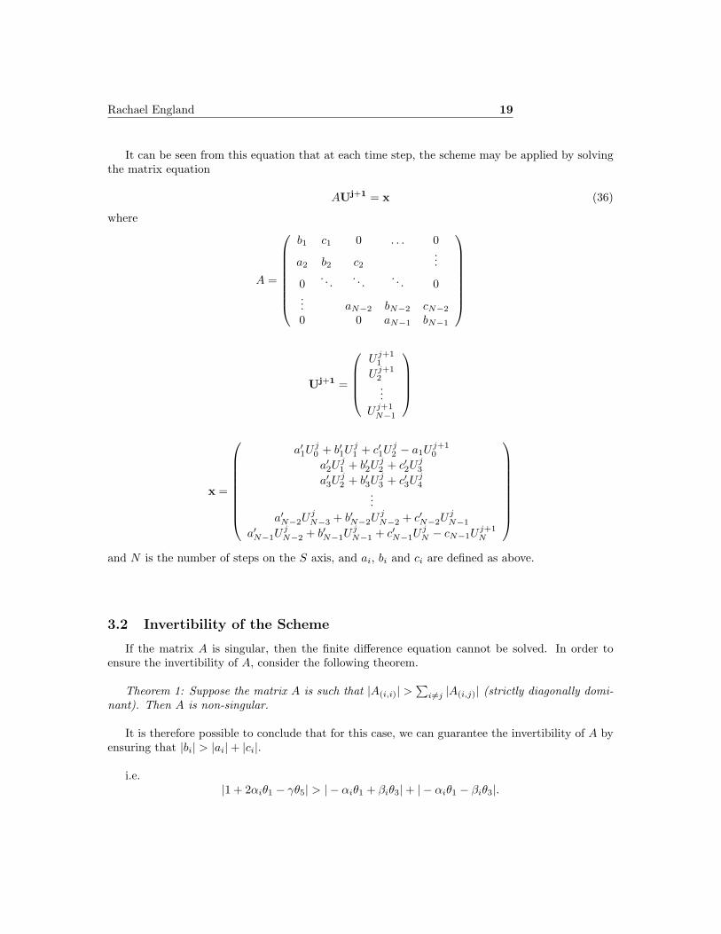
It can be seen from this equation that at each time step, the scheme may be applied by solvingthe matrix equation
AUj+1 = x (36)
where
A =
b1 c1 0 . . . 0
a2 b2 c2
...
0. . . . . . . . . 0
... aN−2 bN−2 cN−2
0 0 aN−1 bN−1
Uj+1 =
U j+1
1
U j+12...
U j+1N−1
x =
a′1Uj0 + b′1U
j1 + c′1U
j2 − a1U
j+10
a′2Uj1 + b′2U
j2 + c′2U
j3
a′3Uj2 + b′3U
j3 + c′3U
j4
...a′N−2U
jN−3 + b′N−2U
jN−2 + c′N−2U
jN−1
a′N−1UjN−2 + b′N−1U
jN−1 + c′N−1U
jN − cN−1U
j+1N
and N is the number of steps on the S axis, and ai, bi and ci are defined as above.
3.2 Invertibility of the Scheme
If the matrix A is singular, then the finite difference equation cannot be solved. In order toensure the invertibility of A, consider the following theorem.
Theorem 1: Suppose the matrix A is such that |A(i,i)| >∑
i 6=j |A(i,j)| (strictly diagonally domi-nant). Then A is non-singular.
It is therefore possible to conclude that for this case, we can guarantee the invertibility of A byensuring that |bi| > |ai|+ |ci|.
i.e.|1 + 2αiθ1 − γθ5| > | − αiθ1 + βiθ3|+ | − αiθ1 − βiθ3|.

Rachael England 20
By the definitions given in (32), it can be seen that αi, βi > 0 and γi < 0. Hence, this equationis true if and only if
1 + 2αiθ1 − γiθ5 > αiθ1 + βitheta3 + | − αiθ1 + βiθ3|.
Therefore, we require one of the following two conditions to be fulfilled:
αiθ1 > βiθ3 (37)
orαiθ1 < βiθ3,
1− γiθ5 > 2(βiθ3 − αiθ1).
3.3 Accuracy
The truncation error Φji is a measure of the discretisation error of the scheme; i.e. the er-
ror in approximating one step of the equation. This can be measured using the equation Φji =
Lji (U − U j
i )Lji (U) where Lj
i (U) represents the application of the numerical scheme to U .
In this case, this becomes
Φji = − 1
δτ
(U(Si, τj + δτ)− U(Si, τj)
)+σ2S2
i
2δS2
[θ1
(U(Si − δS, τj + δτ)− 2U(Si, τj + δτ) + U(Si + δS, τj+δτ )
)+θ2
(U(Si + δS, τj)− 2U(Si, τj) + U(Si − δS, τj)
)]+ rSi
2δS
[θ3
(U(Si + δS, τj + δτ)− U(Si − δS, τj + δτ)
)+ θ4
(U(Si + δS, τj)− U(Si − δS, τj)
)]−r
[θ5U(Si, τj + δτ) + θ6U(Si, τj)
]and using Taylor’s theorem, we can expand around U(Si, τj) to obtain
Φji = − 1
δτ
(U + δτUτ + δτ2
2 Uττ + . . .− U)
σ2S2i
2δS2
[θ1
(U(S, τ + δτ)− δSUS(S, τ + δτ) + δS2
2 USS(S, τ + δτ)− δS3
6 USSS(S, τ + δτ)
+ δS4
24 USSSS(S, τ + δτ) + . . .− 2U(S, τ + δτ) + U(S, τ + δτ) + δSUs(S, τ + δτ)+ δS2
2 USS(S, τ + δτ) + δS3
6 USSS(S, τ + δτ) + δS4
24 USSSS(S, τ + δτ) + . . .)
+θ2
(U − δSUS + δS2
2 USS − δS3
6 USSS + δS4
24 USSSS + . . .− 2U
+U + δSUS + δS2
2 USS + δS3
6 USSS + δS4
24 USSSS + . . .)]
+ rSi
2δS
[θ3
(U(S, τ + δτ) + δSUS(S, τ + δτ) + δS2
2 USS(S, τ + δτ) + δS3
6 USSS(S, τ + δτ) + . . .
−U(S, τ + δτ) + δSUs(S, τ + δτ)− δS2
2 USS(S, τ + δτ) + δS3
6 USSS(S, τ + δτ)− . . .)
+θ4
(U + δSUS + δS2
2 USS + δS3
6 USSS + . . .− U
+δSUS − δS2
2 USS + δS3
6 USSS − . . .)]− r
[θ5
(U + δτUt + δτ2
2 Uττ + . . .)
+ θ6U ].
Rachael England 21
Remembering that θ1+θ2 = θ3+θ4 = θ5+θ6 = 1 and using equation (29), this can be simplifiedto
Φji = −δτ
2Uττ+
σ2S2δS2
24USSSS+
σ2S2θ1δτ
2USSτ+
rSδS2
6USSS+rSθ−3δτUSτ−rθ5δτUτ+higher order terms.
(38)Hence, this numerical approximation is accurate to first order time, second order asset price.
3.4 Stability
If a scheme is unstable, small errors will blow up at each application of the scheme; so thesolution will not be accurate, even if truncation error is small.
As this equation is in a similar form as the diffusion equation, its stability can be calculatedusing fourier stability applied locally - i.e. the condition must be satisfied over all points within thesolution domain.
We let U ji = Λje−zniδS where z =
√−1 and n is an arbitrary constant, and substitute this
expression into the numerical scheme. In order for the scheme to be stable, |Λ| must be less than 1.
Therefore in this case, it is necessary to choose values of θi and δS, δτ such that
|a′ie−znδS + b′i + c′ieznδS | < |aie
−znδS + bi + cieznδS | (39)
for all i.
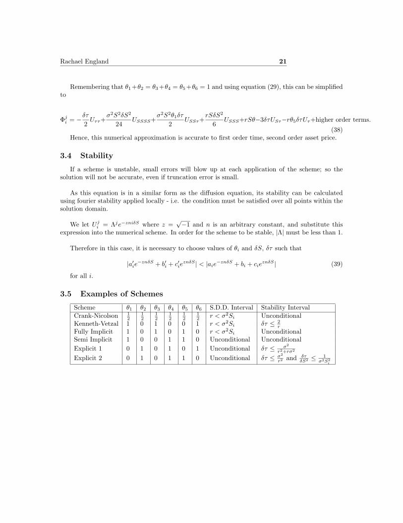
3.5 Examples of Schemes
Scheme θ1 θ2 θ3 θ4 θ5 θ6 S.D.D. Interval Stability IntervalCrank-Nicolson 1
212
12
12
12
12 r < σ2Si Unconditional
Kenneth-Vetzal 1 0 1 0 0 1 r < σ2Si δτ ≤ 2r
Fully Implicit 1 0 1 0 1 0 r < σ2Si UnconditionalSemi Implicit 1 0 0 1 1 0 Unconditional UnconditionalExplicit 1 0 1 0 1 0 1 Unconditional δτ ≤ σ2
r2+rσ2
Explicit 2 0 1 0 1 1 0 Unconditional δτ ≤ σ2
r2 and δτδS2 ≤ 1
σ2S2i
Rachael England 22
4 Inclusion of Stochastic Volatility
We shall now examine the Heston model and numerically solve the partial differential equationusing the same θ method as before. Stella Christodoulou[6] also tried to solve this equation; however,she used transformations to create a finite difference equation which could be solved using thealternating direction implicit algorithm. We shall instead attempt to solve the differential equationover the entire (S, τ) domain simultaneously. Hence, such a transformation is not required.
4.1 Obtaining the Partial Differential Equation
Using the amended model for the asset price as suggested in the introduction, we can now per-form a similar analysis to before to obtain a new differential equation.
Let U = U(S, v, t) represent the value of the derivative at time t according to the price of theunderlying asset. Then by Taylor’s theorem
dU = U(S + dS, v + dv, t + dt)− U(S, v, t)= ∂U
∂t (S, v, t)dt + ∂U∂S (S, v, t)dS + ∂U
∂v (S, v, t)dv + 12
∂2U∂S2 (S, v, t)(dS)2
+ 12
∂2v∂v2 (S, v, t)(dv)2 + ∂2U
∂S∂v (S, v, t)dSdv + O(dt32 ).
(40)
By equation (9) and discarding terms of order dt32 as before, dS2 can be calculated as
(dS)2 = vS2dt. (41)
Similarly, (10) can be used to obtain the equation
(dv)2 = σ2vdt (42)
and a similar process can be used which results in the expression
dSdv = σSvdW1dW2 = σSvρdt (43)
where ρ represents the correlation between the two Wiener processes W1 and W2.
Equations (9), (41), (42) and (43) can then be substituted back into (40), which can then berearranged to get
dU =√
vS∂U
∂SdW1+σ
√v∂U
∂vdW2+(
∂U
∂t+µS
∂U
∂S+k[θ−v]
∂U
∂v+
12S2v
∂2U
∂S2+σSvρ
∂(2)U∂S∂v
+12σ2v
∂2U
∂V 2)dt.
(44)

Rachael England 23
We can now construct a portfolio by buying one derivative and selling ∆ lots of the underlyingasset. Then the value of the portfolio Π is given by
Π = U −∆S. (45)
The rate of change of the value of the portfolio can therefore be given by
dΠ = dU −∆dS
and substituting (9) and (44) into this equation and setting ∆ = ∂U∂S as before gives
dΠ = (∂U
∂t+ k[θ − v]
∂U
∂v+
12vS2 ∂2U
∂S2+ σSvρ
∂2U
∂v∂S+
12σ2v
∂2U
∂v2)dt + σ
√v∂U
∂vdW2. (46)
The random term in W2 can be replaced by −λ(t, S, v)∂U∂v dt where lambda is called the ’price of
volatility risk’, and represents the extra amount of capital return that the investor in the derivativeexpects to gain in exchange for taking on the risk. It is a measurement of how risk averse investorsare likely to be; we shall assume that λ = 0.
As the random term has now vanished, this portfolio is risk free, and by the law of one pricemust therefore grow at the risk free rate. Hence
dΠ = rΠdt= r(U − S ∂U
∂S )dt.(47)
The two equations (46) and (47) can then be set equal, rearranged, and divided by dt to get
12vS2 ∂2U
∂S2+ ρσvS
∂2U
∂S∂v+
12σ2v
∂2U
∂v2+ rs
∂U
∂S+ k[θ − v(t)]
∂U
∂v− rU +
∂U
∂t= 0. (48)
This is the Heston model. It is possible to solve this analytically for financial derivatives witha simple payoff using a transformation of variables to transform this into a parabolic equation.However, it is often not possible to find a solution in this manner when dealing with exotic derivativesas the payoff equations are much more complex. Instead, we shall once again use numerical methodsto solve this model, and the result may be validated by applying the schemes to the more standardoptions.
4.2 The Theta Scheme
As before, we will first transform equation (48) by setting τ = T − t where T is the maturitytime of the derivative. This way we can step forward through the τ variable instead of backwardsthrough time. By doing this, equation (48) becomes
12vS2 ∂2U
∂S2+ ρσvS
∂2U
∂S∂v+
12σ2v
∂2U
∂v2+ rs
∂U
∂S+ k[θ − v(t)]
∂U
∂v− rU =
∂U
∂τ. (49)
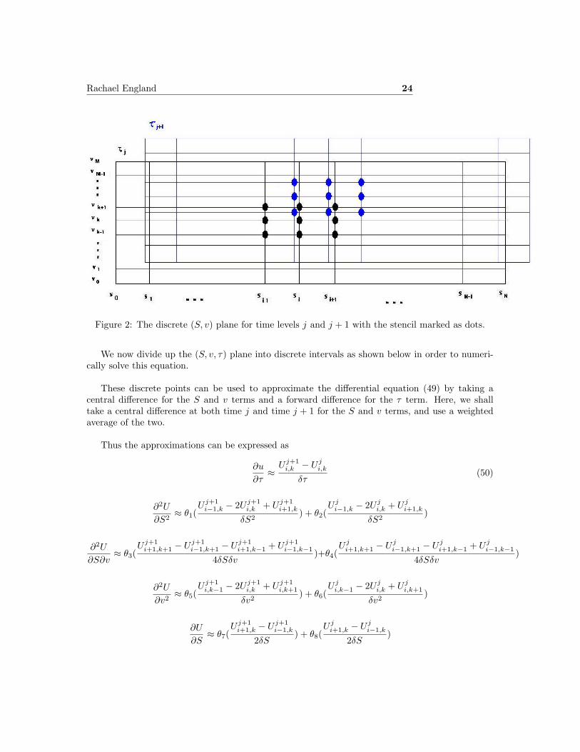
Rachael England 24
Figure 2: The discrete (S, v) plane for time levels j and j + 1 with the stencil marked as dots.
We now divide up the (S, v, τ) plane into discrete intervals as shown below in order to numeri-cally solve this equation.
These discrete points can be used to approximate the differential equation (49) by taking acentral difference for the S and v terms and a forward difference for the τ term. Here, we shalltake a central difference at both time j and time j + 1 for the S and v terms, and use a weightedaverage of the two.
Thus the approximations can be expressed as
∂u
∂τ≈
U j+1i,k − U j
i,k
δτ(50)
∂2U
∂S2≈ θ1(
U j+1i−1,k − 2U j+1
i,k + U j+1i+1,k
δS2) + θ2(
U ji−1,k − 2U j
i,k + U ji+1,k
δS2)
∂2U
∂S∂v≈ θ3(
U j+1i+1,k+1 − U j+1
i−1,k+1 − U j+1i+1,k−1 + U j+1
i−1,k−1
4δSδv)+θ4(
U ji+1,k+1 − U j
i−1,k+1 − U ji+1,k−1 + U j
i−1,k−1
4δSδv)
∂2U
∂v2≈ θ5(
U j+1i,k−1 − 2U j+1
i,k + U j+1i,k+1
δv2) + θ6(
U ji,k−1 − 2U j
i,k + U ji,k+1
δv2)
∂U
∂S≈ θ7(
U j+1i+1,k − U j+1
i−1,k
2δS) + θ8(
U ji+1,k − U j
i−1,k
2δS)
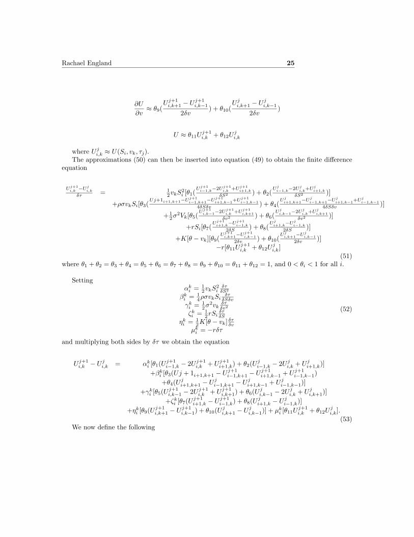
Rachael England 25
∂U
∂v≈ θ9(
U j+1i,k+1 − U j+1
i,k−1
2δv) + θ10(
U ji,k+1 − U j
i,k−1
2δv)
U ≈ θ11Uj+1i,k + θ12U
ji,k
where U ji,k ≈ U(Si, vk, τj).
The approximations (50) can then be inserted into equation (49) to obtain the finite differenceequation
Uj+1i,k
−Uji,k
δτ = 12vkS2
i [θ1(Uj+1
i−1,k−2Uj+1
i,k+Uj+1
i+1,k
δS2 ) + θ2(Uj
i−1,k−2Uj
i,k+Uj
i+1,k
δS2 )]
+ρσvkSi[θ3(Uj+1i+1,k+1−Uj+1
i−1,k+1−Uj+1i+1,k−1+Uj+1
i−1,k−14δSδv ) + θ4(
Uji+1,k+1−Uj
i−1,k+1−Uji+1,k−1+Uj
i−1,k−14δSδv )]
+ 12σ2Vk[θ5(
Uj+1i,k−1−2Uj+1
i,k+Uj+1
i,k+1δv2 ) + θ6(
Uji,k−1−2Uj
i,k+Uj
i,k+1δv2 )]
+rSi[θ7(Uj+1
i+1,k−Uj+1
i−1,k
2δS ) + θ8(Uj
i+1,k−Uj
i−1,k
2δS )]
+K[θ − vk][θ9(Uj+1
i,k+1−Uj+1i,k−1
2δv ) + θ10(Uj
i,k+1−Uji,k−1
2δv )]−r[θ11U
j+1i,k + θ12U
ji,k]
(51)where θ1 + θ2 = θ3 + θ4 = θ5 + θ6 = θ7 + θ8 = θ9 + θ10 = θ11 + θ12 = 1, and 0 < θi < 1 for all i.
Settingαk
i = 12vkS2
iδτ
δS2
βki = 1
4ρσvkSiδτ
δSδv
γki = 1
2σ2vkδτδv2
ζki = 1
2rSiδτδS
ηki = 1
2K[θ − vk] δτδv
µki = −rδτ
(52)
and multiplying both sides by δτ we obtain the equation
U j+1i,k − U j
i,k = αki [θ1(U
j+1i−1,k − 2U j+1
i,k + U j+1i+1,k) + θ2(U
ji−1,k − 2U j
i,k + U ji+1,k)]
+βki [θ3(Uj + 1i+1,k+1 − U j+1
i−1,k+1 − U j+1i+1,k−1 + U j+1
i−1,k−1)+θ4(U
ji+1,k+1 − U j
i−1,k+1 − U ji+1,k−1 + U j
i−1,k−1)]+γk
i [θ5(Uj+1i,k−1 − 2U j+1
i,k + U j+1i,k+1) + θ6(U
ji,k−1 − 2U j
i,k + U ji,k+1)]
+ζki [θ7(U
j+1i+1,k − U j+1
i−1,k) + θ8(Uji+1,k − U j
i−1,k)]+ηk
i [θ9(Uj+1i,k+1 − U j+1
i,k−1) + θ10(Uji,k+1 − U j
i,k−1)] + µki [θ11U
j+1i,k + θ12U
ji,k].
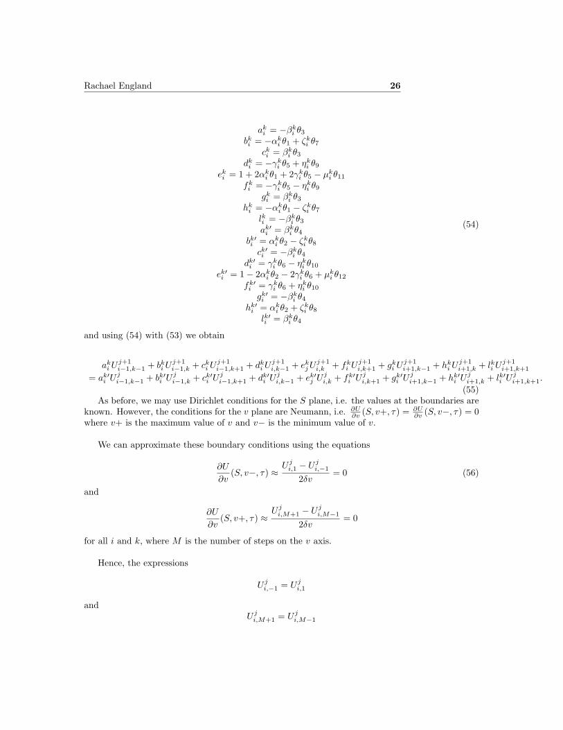
(53)We now define the following
Rachael England 26
aki = −βk
i θ3
bki = −αk
i θ1 + ζki θ7
cki = βk
i θ3
dki = −γk
i θ5 + ηki θ9
eki = 1 + 2αk
i θ1 + 2γki θ5 − µk
i θ11
fki = −γk
i θ5 − ηki θ9
gki = βk
i θ3
hki = −αk
i θ1 − ζki θ7
lki = −βki θ3
ak′i = βk
i θ4
bk′i = αk
i θ2 − ζki θ8
ck′i = −βk
i θ4
dk′i = γk
i θ6 − ηki θ10
ek′i = 1− 2αk
i θ2 − 2γki θ6 + µk
i θ12
fk′i = γk
i θ6 + ηki θ10
gk′i = −βk
i θ4
hk′i = αk
i θ2 + ζki θ8
lk′i = βki θ4
(54)
and using (54) with (53) we obtain
aki U j+1
i−1,k−1 + bki U j+1
i−1,k + cki U j+1
i−1,k+1 + dki U j+1
i,k−1 + ekj U j+1
i,k + fki U j+1
i,k+1 + gki U j+1
i+1,k−1 + hki U j+1
i+1,k + lki U j+1i+1,k+1
= ak′i U j
i−1,k−1 + bk′i U j
i−1,k + ck′i U j
i−1,k+1 + dk′i U j
i,k−1 + ek′j U j
i,k + fk′i U j
i,k+1 + gk′i U j
i+1,k−1 + hk′i U j
i+1,k + lk′i U ji+1,k+1.
(55)As before, we may use Dirichlet conditions for the S plane, i.e. the values at the boundaries are
known. However, the conditions for the v plane are Neumann, i.e. ∂U∂v (S, v+, τ) = ∂U
∂v (S, v−, τ) = 0where v+ is the maximum value of v and v− is the minimum value of v.
We can approximate these boundary conditions using the equations
∂U
∂v(S, v−, τ) ≈
U ji,1 − U j
i,−1
2δv= 0 (56)
and
∂U
∂v(S, v+, τ) ≈
U ji,M+1 − U j
i,M−1
2δv= 0
for all i and k, where M is the number of steps on the v axis.
Hence, the expressions
U ji,−1 = U j
i,1
andU j
i,M+1 = U ji,M−1

Rachael England 27
can be inserted into (55) for all i and j to obtain the equations
b0i U
j+1i−1,0 + (c0
i + a0i )U
j+1i−1,1 + e0
jUj+1i,0 + (f0
i + d0i )U
j+1i,1 + h0
i Uj+1i+1,0 + (l0i + g0
i )U j+1i+1,1
= b0′i U j
i−1,0 + (c0′i + a0′
i )U ji−1,1 + e0′
j U ji,0 + (f0′
i + d0′i )U j
i,1 + h0′i U0
i+1,0 + (l0′i + g0′i )U j
i+1,1
(57)
and
(aMi + cM
i )U j+1i−1,M−1 + bM
i U j+1i−1,M + (dM
i + fMi )U j+1
i,M−1 + eMj U j+1
i,M + (gMi + lmi )U j+1
i+1,M−1 + hMi U j+1
i+1,M
= (aM ′i + cM ′
i )U ji−1,M−1 + bM ′
i U ji−1,M + (dM ′
i + fM ′i )U j
i,M−1 + eM ′j U j
i,M + (gM ′i + lM ′
i )U ji+1,M−1 + hM ′
i U ji+1,M
for the scheme at the boundaries.
As both v and S have two boundary conditions, the scheme must be solved along both directionsat once. We shall do this by solving along the entire (S, τ) grid simultaneously at each successivetime step. It can be seen from these equations that at each time step, this scheme may be appliedby solving the matrix equation
AUj+1 = BUj + x (58)
where
A =
D0 E0 0 . . . 0
C1 D1 E1
...
0. . . . . . . . . 0
... CM−1 DM−1 EM−1
0 ... 0 CM DM
B =
D′0 E′
0 0 . . . 0
C ′1 D′
1 E′1
...
0. . . . . . . . . 0
... C ′M−1 D′
M−1 E′M−1
0 ... 0 C ′M D′
M
U j =
U j1,0
U j2,0...
U jN−1,0
U j1,1
U j2,1...
U jN−1,1
...U j
N−1,M

Rachael England 28
x =
b0′1 U j
0,0 + (c0′1 + a0′
1 )U j0,1 −
(b01U
j+10,0 + (c0
1 + a01)U
j+10,1
)0...0
h0′N−1U
jN,0 + (l0′N−1 + g0′
N−1)UjN,1 −
(h0
N−1Uj+1N,0 + (l0N−1 + g0
N−1)Uj+1N,1
)a1′1 U j
0,0 + b1′1 U j
0,1 + c1′1 U j
0,2 −(a11U
j+10,0 + b1
1Uj+10,1 + c1
1Uj+10,2
)0...
0g1′N−1U
jN,0 + h1′
N−1UjN,1 + l1′N−1U
jN,2 −
(g1
N−1Uj+1N,0 + h1
N−1Uj+1N,1 + l1N−1U
j+1N,2
)......
aM−1′1 U j
0,M−2 + bM−1′1 U j
0,M−1 + cM−1′1 U j
0,M −(aM−11 U j+1
0,M−2 + bM−11 U j+1
0,M−1 + cM−11 U j+1
0,M
)0...0
gM−1′N−1 U j
N,M−2 + hM−1′N−1 U j
N,M−1 + lM−1′N−1 U j
N,M −(gM−1
N−1 U j+1N,M−2 + hM−1
N−1 U j+1N,M−1 + lM−1
N−1 U j+1N,M
)(aM ′
1 + cM ′1 )U j
0,M−1bM ′1 U j
0,M −((aM
1 + cM1 )U j+1
0,M−1 + bM1 U j+1
0,M +)
0...0
(gM ′N−1 + lM ′
N−1)UjN,M−1 + hM ′
N−1UjN,M −
((gM
N−1 + lMN−1)Uj+1N,M−1 + hM
N−1Uj+1N,M
)
and
Ck =
dk1 gk
1 0 . . . 0
ak2 dk
2 gk2
...
0. . . . . . . . . 0
... akN−2 dk
N−2 gkN−2
0 . . . 0 akN−1 dk
N−1
Dk =
ek1 hk
1 0 . . . 0
bk2 ek
2 hk2
...
0. . . . . . . . . 0
... bkN−2 ek
N−2 hkN−2
0 . . . 0 bkN−1 ek
N−1

Rachael England 29
Ek =
fk1 lk1 0 . . . 0
ck2 fk
2 lk2...
0. . . . . . . . . 0
... ckN−2 fk
N−2 lkN−2
0 . . . 0 ckN−1 fk
N−1
for k ∈ {1, 2, ...M − 1},
D0 =
e01 h0
1 0 . . . 0
b02 e0
2 h02
...
0. . . . . . . . . 0
... b0N−2 e0
N−2 h0N−2
0 . . . 0 b0N−1 e0
N−1
E0 =
f01 + d0
1 l01 + g01 0 . . . 0
c02 + a0
2 f02 + d0
2 l02 + g02
...
0. . . . . . . . . 0
... c0N−2 + a0
N−2 f0N−2 + d0
N−2 l0N−2 + g0N−2
0 . . . 0 c0N−1 + a0
N−1 f0N−1 + d0
N−1,
CM =
dM1 + fM
1 gM1 + lM1 0 . . . 0
aM2 + cM
2 dM2 + fM
2 gM2 + lM2
...
0. . . . . . . . . 0
... aMN−2 + cM
N−2 dMN−2 + fM
N−2 gMN−2 + lMN−2
0 . . . 0 aMN−1 + cM
N−1 dMN−1 + fM
N−1
DM =
eM1 hM
1 0 . . . 0
bM2 eM
2 hM2
...
0. . . . . . . . . 0
... bMN−2 eM
N−2 hMN−2
0 . . . 0 bMN−1 eM
N−1;
and

Rachael England 30
C ′k =
dk′1 gk′
1 0 . . . 0
ak′2 dk′
2 gk′2
...
0. . . . . . . . . 0
... ak′N−2 dk′
N−2 gk′N−2
0 . . . 0 ak′N−1 dk′
N−1
D′k =
ek′1 hk′
1 0 . . . 0
bk′2 ek′
2 hk′2
...
0. . . . . . . . . 0
... bk′N−2 ek′
N−2 hk′N−2
0 . . . 0 bk′N−1 ek′
N−1
E′k =
fk′1 lk′1 0 . . . 0
ck′2 fk′
2 lk′2
...
0. . . . . . . . . 0
... ck′N−2 fk′
N−2 lk′N−2
0 . . . 0 ck′N−1 fk′
N−1
for k ∈ {1, 2, ...M − 1},
D′0 =
e0′1 h0′
1 0 . . . 0
b0′2 e0′
2 h0′2
...
0. . . . . . . . . 0
... b0′N−2 e0′
N−2 h0′N−2
0 . . . 0 b0′N−1 e0′
N−1
E′0 =
f0′1 + d0′
1 l0′1 + g0′1 0 . . . 0
c0′2 + a0′
2 f0′2 + d0′
2 l0′2 + g0′2
...
0. . . . . . . . . 0
... c0′N−2 + a0′
N−2 f0′N−2 + d0′
N−2 l0′N−2 + g0′N−2
0 . . . 0 c0′N−1 + a0′
N−1 f0′N−1 + d0′
N−1,

Rachael England 31
C ′M =
dM ′1 + fM ′
1 gM ′1 + lM ′
1 0 . . . 0
aM ′2 + cM ′
2 dM ′2 + fM ′
2 gM ′2 + lM ′
2
...
0. . . . . . . . . 0
... aM ′N−2 + cM ′
N−2 dM ′N−2 + fM ′
N−2 gM ′N−2 + lM ′
N−2
0 . . . 0 aM ′N−1 + cM ′
N−1 dM ′N−1 + fM ′
N−1
D′M =
eM ′1 hM ′
1 0 . . . 0
bM ′2 eM ′
2 hM ′2
...
0. . . . . . . . . 0
... bM ′N−2 eM ′
N−2 hM ′N−2
0 . . . 0 bM ′N−1 eM ′
N−1,
N is the number of steps on the S axis, M the number of steps on the v axis, and ak
i , bki , etc. are
defined as above.
4.3 Invertibility of the Scheme
If the matrix A is singular, then the finite difference equation cannot be solved. Using the sametheorem as before, we can guarantee the invertibility of A by ensuring that |ek
i | > |aki |+ |bk
i |+ |cki |+
|dki |+ |fk
i |+ |gki |+ |hk
i |+ lki .
i.e.
|1 + 2αki θ1 + 2γk
i θ5 − µki θ11| > | − βk
i θ3|+ | − αki θ1 + ζiθ7|+ |βk
i θ3|+ | − γki θ5 + ηk
i θ9|+| − γk
i θ5 − ηki θ9|+ |βk
i θ3|+ | − αki θ1 − ζk
i θ7|+ |βki θ3|.
By the definitions given in (52), it can be seen that αi, βi, γki , ζk
i > 0 and µki < 0. It is also
assumed that ηki > 0 as it is not possible to have a negative volatility. Hence, this equation is true
if and only if
1+2αki θ1+2γk
i θ5−µki θ11| > 4βk
i θ3+|−αki θ1+ζk
i theta7+αki θ1+ζk
i θ7+|−γki θ5+ηk
i θ9|+γki θ5+ηk
i θ9.
Consider the following four cases.
1. Suppose αki θ1 < ζk
i θ7, γki θ5 < ηk
i θ7.
Then we require that
1 + 2αki θ1 + 2γk
i θ5 − µki θ11| > 4βk
i θ3 + 2ζki θ7 + 2ηk
i θ9. (59)
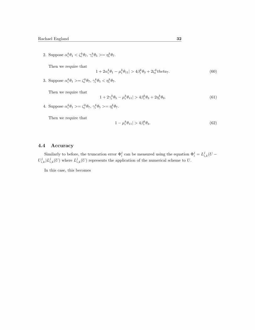
Rachael England 32
2. Suppose αki θ1 < ζk
i θ7, γki θ5 >= ηk
i θ7.
Then we require that1 + 2αk
i θ1 − µki θ11| > 4βk
i θ3 + 2ζki theta7. (60)
3. Suppose αki θ1 >= ζk
i θ7, γki θ5 < ηk
i θ7.
Then we require that1 + 2γk
i θ5 − µki θ11| > 4βk
i θ3 + 2ηki θ9. (61)
4. Suppose αki θ1 >= ζk
i θ7, γki θ5 >= ηk
i θ7.
Then we require that1− µk
i θ11| > 4βki θ3. (62)
4.4 Accuracy
Similarly to before, the truncation error Φji can be measured using the equation Φj
i = Lji,k(U −
U ji,k)Lj
i,k(U) where Lji,k(U) represents the application of the numerical scheme to U .
In this case, this becomes

Rachael England 33
Φji,k = − 1
δτ
(U(Si, vk, τj + δτ)− U(Si, τj)
)+VkS2
i
2δS2
[θ1
(U(Si − δS, vk, τj + δτ)− 2U(Si, vk, τj + δτ) + U(Si + δS, vk, τj + δτ)
)+θ2
(U(Si − δS, vk, τj)− 2U(Si, vk, τj) + U(Si + δS, vk, τj)
)]+ ρvkSi
4δSδv
[θ3
(U(Si + δS, vk + δv, τj + δτ)− U(Si − δS, vk + δv, τj + δτ)
−U(Si + δS, vk − δv, τj + δτ) + U(Si − δS, vk − δv, tj + δt))
+θ4
(U(Si + δS, vk + δv, τj)− U(Si − δS, vk + δv, τj)
−U(Si + δS, vk − δv, τj) + U(Si − δS, vk − δv, tj))]
+σ2vk
2δv2
[θ5
(U(Si, vk − δv, τj + δτ)− 2U(Si, vk, τj + δτ) + U(Si, vk + δv, τj + δt)
)+θ6
(U(Si, vk − δv, τj)− 2U(Si, vk, τj) + U(Si, vk + δv, τj)
)]+ rSi
2δS
[θ7
(U(Si + δS, vk, τj + δτ)− U(Si − δS, vk, τj + δτ)
)+θ8
(U(Si + δS, vk, τj)− U(Si − δS, vk, τj)
)]+K[θ−vk]
2δv
[θ9
(U(Si, vk + δv, τj + δτ)− U(Si, vk − δv, τj + δt)
)+θ10
(U(Si, vk + δv, τj)− U(Si, vk − δv, τj)
)]−r
[θ11U(Si, vk, τj + δτ) + θ12U(Si, vk, τj)
]and using Taylor’s theorem, we can expand around U(Si, τj) to obtain

Rachael England 34
Φji,k = − 1
δτ
(U + δτUτ + δτ2
2 Uττ + . . .− U)
+VkS2i
2δS2
[θ1
(U(S, v, τ + δτ)− δSUs(S, v, τ + δτ) + δS2
2 US(S, v, τ + δτ)− δS3
6 uSSS(S, v, τ + δτ)
+ δS4
24 USSSS(S, v, τ + δτ) + . . .− 2U(S, v, τ + δτ) + U(S, v, τ + δτ) + δSUS(S, v, τ + δτ)+ δS2
2 USS(S, v, τ + δτ) + δS3
6 USSS(S, v, τ + δτ) + δS4
24 USSSS(S, v, τ + δτ) + . . .)
+θ2
(U − δSUS + δS2
2 USS − δS3
6 USSS + δS4
24 + . . .− 2U
+U + δSUS + δS2
2 USS + δS3
6 USSS + δS4
24 USSSS + . . .)]
+ ρvkSi
4δSδv
[θ3
(4δSδvUSv(S, v, τ + δτ) + 2δsδv3
3 USvvv(S, v, τ + δτ) + 2δsav3 USSSv(S, v, τ + δτ) + . . .
)+θ4
(4δSδvUSv + 2δSδv3
3 USvvv + 2δS3δv3 USSSv + . . .
)]+σ2vk
2δv2
[θ5
(U(S, v, τ + δτ)− δvUv(S, v, τ + δτ) + δv2
2 Uvv(S, v, τ + δτ)− δv3
6 Uvvv(S, v, τ + δτ)
+ δv4
24 Uvvvv(S, v, τ + δτ) + . . .− 2U(S, v, τ + δτ) + U(S, v, τ + δt) + δvUv(S, v, τ + δτ)+ δ v2
2 Uvv(S, v, τ + δτ) + δv3
6 Uvvv(S, v, τ + δτ) + δv4
24 Uvvvv(S, v, τ + δτ) + . . .)
+θ6
(U − δvUv + δv2
2 Uvv − δv3
6 Uvvv + δv4
24 Uvvvv + . . .
−2U + U + δvUvv + δv2
2 Uvv + δv3
6 Uvvv + δv4
24 Uvvvv + . . .)]
+ rSi
2δS
[θ7
(U(S, v, τ + δτ) + δSUS(S, v, τ + δτ) + δS2
2 USS(S, v, τ + δτ) + δS3
6 USSS(S, v, τ + δτ) + . . .
−U(S, v, τ + δτ) + δSUSS, v, τ + δτ)− δS2
2 USS(S, v, τ + δτ) + δS3
6 USSS(S, v, τ + δτ) + . . .)
+θ8
(U + δSUS + δS2
2 USS + δS3
6 USSS + . . .− U + δSUS − δS2
2 USS + δS3
6 USSS + . . .)]
+K[θ−vk]2δv
[θ9
(U(S, v, τ + δτ) + δvUv(S, v, τ + δτ) + δv2
2 Uvv(S, v, τ + δτ) + δv3
6 Uvvv(s, v, τ + δτ) + . . .
−U(S, v, τ + δt) + δvUv(S, v, τ + δτ)− δv2
2 Uvv(S, v, τ + δτ) + δv3
6 Uvvv(S, v, τ + δτ) +)
+θ10
(U + δvUv + δv2
2 Uvv + δv3
6 Uvvv + . . .− U + δvUv − δv2
2 Uvv + δv3
6 Uvvv + . . .)]
−r
[θ11
(U + δτUτ + . . .
)+ θ12U
]Remembering that θ1 + θ2 = θ3 + θ4 = θ5 + θ6 = θ7 + θ8 = θ9 + θ10 = θ11 + θ12 = 1 and using
equation (49), this can be simplified to
Φji = − δτ
2 Utt + vS2
2 ( δS2
12 USSSS + θ1δτUSSt) + ρσvS( δv2
6 USvvv + δv2
6 USSSv + θ3δτUSvτ )+fracσ2v2( δv2
12 Uvvvv + θ5δτUvvτ ) + rS( δS2
6 USSSS + θ7δτUSτ + K[θ − v]( δv2
2 Uvvv
+θ9δτUvτ )− θ11rδτUτ ) + higher order terms.(63)
Hence, this numerical approximation is accurate to first order time, second order asset price andvolatility.

Rachael England 35
4.5 Stability
Similarly to before, we shall use Fourier stability for this scheme. Let U ji,k = Λje−zniδSe−zmkδv
where z =√−1 and n, m are arbitrary constants, and substitute this expression into the numerical
scheme. In order for the scheme to be stable, |Λ| must be less than 1.
Therefore in this case, it is necessary to choose values of θi and δS, δτ such that
|ak′i e−z(nδS+mδv) + bk′
i e−znδS + ck′i ez(mδv−nδS) + dk′
i e−zmδv + ek′i
+fk′i ezmδv + gk′
i ez(nδS−δvm) + hk′i eznδS + lk′i ez(nδS+mδv)
<|ak
i e−z(nδS+mδv) + bki e−znδS + ck
i ez(mδv−nδS) + dki ezmδv + ek
i
+fki ezmδv + gk
i ez(nδS−δvm) + hki eznδS + lki ez(nδS+mδv)|
(64)
for all i.
4.6 Examples of Schemes
Scheme θ1 θ2 θ3 θ4 θ5 θ6 θ7 θ8 θ9 θ10 θ11 θ12
Crank-Nicolson 12
12
12
12
12
12
12
12
12
12
12
12
Kenneth-Vetzal 1 0 1 0 1 0 1 0 1 0 0 1Fully Implicit 1 0 1 0 1 0 1 0 1 0 1 0Scheme S.D.D. Interval Stability IntervalCrank-Nicolson vkSi > r, σ2vk > K[θ − vk]− λj
i,k, 2−rvkSi
> ρσ UnconditionalKenneth-Vetzal vkSi > r, σ2vk > K[θ − vk]− λj
i,k, 1−rvkSi
> ρσ (σ2vk + K[θ − v − k])(r + vkSi) > ρσvk
δτ
Fully Implicit vkSi > r, σ2vk > K[θ − vk]− λji,k, 1−r
vkSi> ρσ (σ2vk + K[θ − v − k])(r + vkSi) > ρσvk
δτ

Rachael England 36
5 Further Work: Inclusion of Bond Price
Bond prices are very sensitive to interest rates, and are often used to measure them. We shalltherefore try and use them in our model so as to incorporate stochastic interest rates into the pricingproblem[4]. Possible methods of solving this are left for future work.
5.1 Derivation of Partial Differential Equation
We begin assuming that the prices of the underlying asset and the bond are governed by theequations
dS = µSSdt + σSdt + σS(t)√
v(t)SdW1
dP = µP Pdt + σP (t)√
v(t)PdW2(65)
where both values depend upon the same variable v(t), and W1 and W2 represent Wiener processesas before. The bond used must be chosen carefully to ensure that this is a valid assumption.
We use the same model as before for the volatility v; i.e.
dv = K[θ − v]dt + 2σ√
vdW3. (66)
Let U = U(S, P, v, t) represent the value of the derivative at time t according to the price of theunderlying asset. Then by Taylor’s theorem
dU = U(S + dS, P + dP, v + dv, t + dt)− U(S, v, t)= ∂U
∂t (S, P, v, t)dt + ∂U∂S (S, P, v, t)dS + ∂U
∂P (S, P, v, t)dP + ∂U∂v (S, v, t)dv
+ 12
∂2U∂S2 (S, v, t)(dS)2 + 1
2partial2U
∂s∂P (S, P, v, t)dP 2 + 12
∂2v∂v2 (S, P, v, t)(dv)2 + ∂2U
∂S∂v (S, v, t)dSdv
+ ∂2U∂P∂v dPdv + ∂2U
∂S∂P dSdP + O(dt32 ).
(67)By equations (65) and (66), and discarding terms of order dt
32 as before, we calculate
dS2 = σ2SvS2dt
dP 2 = σ2P vP 2dt
dv2 = σ2vdtdSdv = σSσvSρS,vdtdPdv = σP σvPρP,vdt
dSdP = σSσP vSPρS,P dt
(68)
where ρS,v represents the correlation between the processes W1 and W3, ρP,v represents the corre-lation between the processes W2 and W3, and ρS,P represents the correlation between the processesW1 and W2.

Rachael England 37
Equations (65), (66), and (68) can then be substituted back into (67), which can then berearranged to get
dU = σS√
vS ∂U∂S dW1 + σP
√vP ∂U
∂P dW2 + σ√
v ∂U∂v dW3 + (∂U
∂t + µS ∂U∂S + µP ∂U
∂P + k[θ − v]∂U∂v
+ 12σ2
SS2v ∂2U∂S2 + 1
2σ2v ∂2U∂V 2 + 1
2σ2P vP 2 ∂2U
∂P 2 + σSσSvρS,v∂(2)U∂S∂v + σP σvPρP,v
∂2U∂P∂v + σSσP vSPρS,P
∂2U∂S∂P )dt.
(69)We can now construct a portfolio by buying one derivative and selling ∆1 lots of the underlying
asset and ∆2 lots of the bond. Then the value of the portfolio Π is given by
Π = U −∆1S −∆2P. (70)
The rate of change of the value of the portfolio can therefore be given by
dΠ = dU −∆1dS −∆2dP
and substituting (65) into this equation and setting ∆1 = ∂U∂S and ∆2 = ∂U
∂P gives
dΠ = σ√
v ∂U∂v dW3 + (∂U
∂t + k[θ − v]∂U∂v + 1
2σ2SS2v ∂2U
∂S2 + 12σ2v ∂2U
∂V 2 + 12σ2
P vP 2 ∂2U∂P 2
+σSσSvρS,v∂(2)U∂S∂v + σP σvPρP,v
∂2U∂P∂v + σSσP vSPρS,P
∂2U∂S∂P )dt.
(71)
The random term in W2 can be replaced as before by −λ(t, S, v)∂U∂v dt where lambda is the price
of volatility risk. As the random term has now vanished, this portfolio is risk free, and by the lawof one price must therefore grow at the risk free rate. Hence
dΠ = rΠdt= r(U − S ∂U
∂S − P ∂U∂P )dt.
(72)
The two equations (70) and (72) can then be set equal, rearranged, and divided by dt to get
12σ2
SS2v ∂2U∂S2 + 1
2σ2P vP 2 ∂2U
∂P 2 + 12σ2v ∂2U
∂v2 + σSσP vSPρS,P∂2U
∂S∂P + σSσSvρS,v∂(2)U∂S∂v
+σP σvPρP,v∂2U
∂P∂v + rS ∂U∂S + rP ∂U
∂P + k[θ − v]∂U∂v − rU + ∂U
∂t= 0.
(73)
5.2 Theta Method
The obvious route to take when solving the bond model would be to use the same sort of θmethod as before. However, as the new model is in three dimensions this would necessitate thesolving of a series of finite difference equations across the entire (S, P, v) plane for each time step.A program written to perform this task would be extremely slow and therefore of little practicaluse to derivatives traders, who need values quickly when dealing in the financial market. This couldperhaps be solved by using explicit methods only, although great care would have to be taken toensure stability, or by using larger step sizes in all directions, which may lead to a loss in accuracysuch that the model beomes less correct than the application of the previous two models.

Rachael England 38
5.3 Alternating Direction Implicit Method
Another possible way of numerically solving this model might be to employ the alternating di-rection implicit method (or A.D.I.)[7]. In two dimensions, this method involves taking an explicitfinite difference in one spatial dimension and an implicit finite difference in the other, at a timelevel j + 1
2 . The difference methods are then alternated between each dimension for each half timelevel, and rearranged to eliminate the solution at j + 1
2 . It might be possible to extend this methodto three dimensions, either by alternating in three different directions, or by alternating betweentwo of the three dimensions and a third and hence solving over a two dimensional grid for each stepas before.
We also note here that in order to employ the A.D.I. method, it is necessary to first eliminatethe terms which contain derivatives with respect to variables in more than one direction, e.g. ∂2U
∂S∂P .To do this the equation must be transformed into new co-ordinates. The new frame of referencemay also require a non-uniform grid to be applied when using the finite difference methods.
5.4 Finite Element Method
An alternative approach may be to solve the new model using finite element instead of finitedifference methods. The idea behind these methods is to find a piecewise linear solution to adifferential equation, which can be made to approximate the solution in an integrational sense byintegrating the terms in the equation until only U or ∂U
∂x remain. The piecewise linear solutioncan then be substituted into the resultant equation and solved to obtain the answer. For Dirichletconditions, the solutions at the nodes are equal to the analytical answer. In the case of the modelderived in this section, three dimensional elements are required when solving the equation.
5.5 Finite Volume Method
An alternative approach may be to solve the new model using finite volume instead of finitedifference methods. Finite volume methods involve breaking down the domain into control volumes,for example volumes centred on each U j
i,k whose boundaries stretch for half a step in all directions,and then discretising the integral form of the differential equation. This is suggested as a possibleextension because most of the initial conditions for financial derivatives involve a discontinuousderivative; such features are better approximated by finite volume methods than finite differencemethods.
5.6 Comparison with Monte Carlo Simulations
Monte Carlo methods[9] are widely used in the fields of banking and insurance, as well as nu-merous other fields containing non-deterministic models. The idea of a Monte Carlo method isto specify an initial condition along with a series of stochastic equation with a given distribution.The algorithm then generates random numbers according to the distribution and evolves the modelaccordingly; repeating this process thousands of times should give a reasonable distribution of theexpected final solution.

Rachael England 39
Monte Carlo methods are computationally very expensive to use, although the idea is a simpleone and easy to program, and the execution may be speeded up application of techniques such asvariance reduction. We propose that future work could include setting up a Monte Carlo methodto mimic empirical data and then comparing the results to the deterministic pricing models derivedin this project.

Rachael England 40
6 Algorithms for solving the equations
In this section we consider how to write and structure the programs required for solvng themodels using the finite difference schemes outlined earlier.
6.1 Matrix Inversion
In order to solve the equations at each time step, it is necessary to calculate the value of A−1 xright hand side vector (rhs).
For the Black-Scholes numerical approximations, A is tri-diagonal. It can therefore be solvedusing the Thomas Algorithm, which works as follows:
Let A = LR where
L =
1l2 1
. . . . . .lN−1 1
R =
r1 c1
. . . . . .rm−2 cN−21
rN−1
and
r1 = b1
ri+1 = (bi+1 − ai+1ci)/ri
li+1 = ai+1/ri.
Firstly, let y = RA−1
Thus:Ly = rhs
This can be solved for y, giving:
y(1) = rhs(1)and for i = 2,3, ... m-1

Rachael England 41
y(i) = rhs(i)− li−1yi−1
Finally, the equation RA−1 = y can be solved to give:
solution(m− 1) = y(m− 1)/rN−1
and for i = N-2, N-3, ... 1solution(i) = (y(i)− cisolution(i + 1))/ri.
However, for the Heston solver, the matrix is block-tridiagonal, and cannot be solved directly.Instead, we shall solve the equation by using the Gauss-Seidel method, which works as follows:
Firstly, split the matrix A into L−R where:
Li,j ={
Ai,j if j ≤ i0 otherwise
Ri,j ={−Ai,j if j > i
0 otherwise
Suppose Ax = rhs, where rhs is known and x is not. Thus Lx = Rx + b, and an iteration canbe set up such that given some initial guess x0, Lxi+1 = Rxi + b until the iteration homes in onsome value of x.
This algorithm unfortunately is not very efficient, and if the (S, v, τ) grid becomes too large, willtake a long time to run. This is unacceptable when pricing derivatives, as pricing may have to bedone very quickly. It is therefore necessary to sacrifice some of the accuracy, both in the step sizesand in the error tolerance level of the iteration, in order to produce a result within a reasonable time.
For both of these algorithms, only the values in the diagonals shall be stored rather than theentire matrix, as the program will therefore take up much less memory.
6.2 Black-Scholes Solver
The program written for the numerical solution of the Black-Scholes equation works as follows:
1. Define variables and ask user for input
2. If the user has chosen a Swaption, ask for spot rates and calculate value with which to multiplythe final call solution
3. Resize matrices and vectors appropriately
4. Fill in τ and S vectors with step values
5. Fill in the boundary and initial values
6. Define the diagonal entries for A

Rachael England 42
7. Loop through all τ steps and:
I. Define entries in right hand side vector
II. Use the Thomas algorithm to calculate solution
III. Insert solution back into matrix for U
8. Output final row of solution to file to get prices for U at time t = 0.
A copy is included in the Appendix.
6.3 Heston Model Solver
The program written for the numerical solution of the Heston equation works as follows:
1. Define variables and ask user for input
2. If the user has chosen a Swaption, ask for spot rates and calculate value with which to multiplythe final call solution
3. Resize matrices and vectors appropriately
4. Fill in τ , v, and S vectors with step values
5. Fill in the initial values
6. Loop through all τ steps and:
I. Enter in boundary values
II. Define entries of A
III. Define entries in right hand side vector
IV. Use the Gauss-Seidel iteration to calculate solution
V. Insert solution back into for U for that time step
VI. Set previous solution to be new solution for use in the next time step
7. Output final row of solution to file to get prices for U at time t = 0.
A copy is included in the Appendix.

Rachael England 43
7 Results
The first section of results contains a comparison with some of Stella Christodoulou’s[6] resultsfor standard options, and includes the results from the numerical Heston model for comparison.
As an examnination of the numerical approximation, we shall next consider the change in re-sults as the boundaries are moved closer together, and the effect this has on the correctness of thesolution. We shall also vary the step sizes in order to determine what sizes are required for accurateenough values.
Next, we include relevant market data for the pricing of the European Swaptions, along withmarket prices for comparison with the results. This is followed by the prices as calculated by eachof the two numerical programs.
Finally, the numerical models shall be used to price several exotic options, and the solutioncompared to the market values. In order to perform this task correctly the correct parameters mustbe used; and although it is possible to find market data for the values of the current volatility (σfor the Black-Scholes model, θ for the Heston model) and the risk-free interest rate (r) for a givenunderlying share price, values are not given for K, ρ, or σ in the Heston model. The value of σ isa measurement of the volatility of the volatilities, and an appropriate estimate can be calculatedfrom historical data. In order to price an exotic derivative, we have therefore run the model for astandard vanilla option at the strike rate and found values for which the solution is most accurate.The values obtained in this way shall then be used for pricing the exotic derivative.

Rachael England 44
7.1 Comparison with Stella Christodoulous Results

Rachael England 45
7.2 Variation of Boundaries and Step Sizes

Rachael England 46
7.3 Market Information for Volatilities and Forward Rates, and Pricesfor European Swaptions

Rachael England 47
7.4 Pricing of Knock-in Caps and Comparison with Market Data

Rachael England 48
7.5 Discussion of Results
1. Comparison with previous results
The parameters used to produce the results in this table are: S− = 50, S+ = 150, v− = 0.1,v+ = 0.3, T = 0.25, δS = 0.5, δv = 0.005, δτ = 0.01, E = 100, r = 0/08. In the Black-Scholesmodel σ = 0.2; in the Heston model sigma = 4, θ = 0.2, K = 0.5, ρ = −0.95.
The results for the Black-Scholes numerical model are comparable with previous work [6],and are generally accurate enough for the practical purpose of pricing. The error for theCrank-Nicolson scheme is much smaller than the rest, as it is second order in time insteadof first order in time like the other schemes. The explicit schemes however are not stable forthese values. To correct this, the size of δτ must be decreased.
The results for the Heston model however are less accurate. We note that in this case not onlythe numerial approximation itself but also the Gauss-Seidel iteration are sources of error, andspeculate that it is the iteration which is the main source of error here. Reducing the stepsize may help with the error generated by the numerical approximation; however, decreasingthe step sizes in the S and v plane will increase the size of the matrix to be inverted andso slow down the program, and decreasing the step size in the τ plane will also slow downthe program as the inversion must be repeated more times, which will also increase the ef-fect of the error in the iteration. The entries in the matrix A will also be much smaller incomparison to the error tolerance, which will therefore not be small enough to demand therequired accuracy. A possible way of dealing with this would be to vary the error tolerancealong with the step sizes, although the smaller the tolerance the longer each iteration willtake to complete. We also note that the results given as the analytical solution also containsome error, as the closed form for vanilla options contains an integration whose solution hasbeen estimated using numerical methods.
We consider the graphs showing the call and put values for the two models. As the value ofthe correlation ρ is negative, the expected volatility as calculated by the Heston model willbe greater for smaller values of S and less for larger values of S than in the Black-Scholesmodel. For the call graph, the volatility is therefore less than expected by the Black-Scholesmodel for the out-of-the-money prices and the Heston model will thus evaluate these pricesto be less than the Black-Scholes prices, whereas the volatility is less for the in-the-moneyoptions, and hence the Heston model assumes that the option is more likely to finish in-the-money than the Black-Scholes results. Similarly, the in-the-money prices for the put optionis modelled as being more likely to finish out-of-the-money and hence are priced less by theHeston model than in the Black-Scholes, whereas the out-of-the-money prices are modelledas being more likely to result in a positive payoff, and hence are evaluated at a greater pricethan that calculated by the Black-Scholes model.
2. Variation of boundaries
Rachael England 49
The parameters here are the same as those used to produce the results detailed in the previoussection, except that the boundaries have been moved as detailed in the tables.
Considering these results, we note that varying the boundaries makes a difference to the ac-curacy of the results, particularly for those prices nearer to the boundaries. However, thedifference is very slight. For the boundaries in the S plane, accurate enough results can beproduced for the Black-Scholes equation when the boundaries are placed 1
4 of the value of thestrike price away from this value, and for the Heston model at 1
2 of the value away from thesrike price. We shall also set the boundaries for the v plane at 1
4 value spead in each directionaway from the current rate.
3. Variation of step sizes
The parameters here are the same as those used to produce the first set of results, except thatthe step sizes have been changed as detailed in the tables.
We note from the results given here that although halving the size of the S step does approx-imately half the error in the Black-Scholes results, the difference is not necessary for accurateenough results. When the S and v step sizes are halved for the Heston model, not only doesthe program take an unacceptably long time to run, but the errors seem to have increasedrather than decreased. This may be due to the error produced by using the Gauss-Seidel it-eration. The values of δS and δv shall therefore remain at the same values for the productionof the rest of the results.
Decreasing the value of δτ not only gives more accurate resuls for the Black-Scholes model,it also produces stability for the explicit schemes. The value of δτ shall therefore be de-creased to 0.001 for this model. The explicit schemes shall not be used for the remainderof the results, as they are too unstable for use in a commercial environment. Decreasingthe value of δτ for the Heston model does not appear to improve the accuracy, and makesthe program far too slow. The value of δτ = 0.01 shall therefore be maintained for this model.
4. Pricing of swaptions
For this section, we shall use the parameters as determined in the previous two sections.
The results given here by the Black-Scholes numerical solution are comparable to the ana-lytical results; however while the prices for swaptions with early maturities are reasonablyaccurate for the Heston numerical solution, the error becomes very large for those swaptionswith a long term maturity. We also notice that for an underlying swap with a higher maturity(e.g. 4y-7y), any error is multiplied by the inclusion of the A = (
∑mi=1 D(ti)) value.
Rachael England 50
It is clear from the comparison with the market data that the Black-Scholes results are closerto the accepted market price. This is because it is the Black-Scholes model which traderscurrently use as a basis for the price. The model suggested here is believed to be a moreaccurate assessment of the true price, and is therefore more useful when brokers are trying toneutralise the risk associated with the derivative which has already been bought or sold by atrader.
5. Pricing of knock-in caps
A knock-in cap constructed of E1 digitals combined with a call option, both with a strike E2.The payoff is therefore max(S − E2, 0) + E1
max(S−E2,0)S−E2
. The model is used here to price aknock-in cap with a maturity of 1 year of varying strikes for a specific stock. In this case, theunderlying asset price is currently 110.
The volatility curve shown in this section of results shows the market values[8], and parametersshould be used which mimick this graph. Trial and error shows that the requisite parametersfor the Heston model are σ = 4, K = 1, θ = 0.4, and ρ = −0.2. The original volatility is 0.43;this shall be the point at which we take our result, and the value of σ in the Black-Scholessolution. The current value of the risk-free rate is r = 0.045.
Similarly to before, we note that the Black-Scholes solution produces values closer to thetraded prices than the Heston solution. The solutions given by the Heston models also varyconsiderably between the Crank-Nicolson scheme and the other two. Based upon past per-formance, we believe the Crank-Nicolson solution to be more accurate.
As the Heston solution is more useful to a broker than a trader, more time may be taken toproduce the results. We therefore suggest that in the future a much smaller error tolerance isused for the Gauss-Seidel iteration, as this is the greatest source of error but also of inefficiency.
Rachael England 51
8 Summary and Conclusion
During this rsearch we have considered the numerical solution of two models, the Black-Scholesmodel and the Heston model, which are used for pricing financial derivatives. We have used theθ method to find finite difference equations which numerically solve these two models. In orderto solve these equations, we have written them in the form of a single matrix equation. For theBlack-Scholes numerical solution, this matrix equation may be solved directly using the Thomasalgorithm; for the Heston numerical solution, the equation is solved using an iterative process, inthis case the Gauss-Seidel method. The results produced in this way are very accurate for theBlack-Scholes solution, but less accurate for the Heston solution, with the Gauss-Seidel iterationbeing the largest source of error.
As this model would be used within a commercial envronment, it is important to produce theresults within a reasonable period of time. When the maturity is long term, or the error toleranceis increased, the time taken to produce results is greatly increased. The number of step sizes in theS and v planes can only be decreased so far, as the numerical boundaries must be far enough apartto mimic the boundary conditions, and increasing the step size decreases efficiency and stability.
We propose that this model is used for brokers assessing the true value of derivatives, and thatthe error tolerance for the iteration is decreased in this case as more time may be taken to produceresults.
For future work, it is possible to include the Bond price in the partial differential equationused for pricing derivatives. However, using the same θ method in this case is not commerciallyviable. Instead, we propose the use of the alternating direction implicit method, or a differet typeof numerical solution such as a finite element or finite volume method. We also suggest the use ofMonte-Carlo simulations in order to compare the accuracy of the models in terms of price risk.

Rachael England 52
References
[1] John C. Hull, 2000, ”Options, Futures, & Other Derivatives”, fourth edition., Prentice-HalllInternational
[2] F. Black & M. Scholes, 1973, ”The Valuations of Options and Corporate Liabilities”, Journalof Political Economy, 81, 637-654
[3] M. Rubenstein, 1985, ”Nonparametric Tests of Alternative Option Pricing Models Using AllReported Trades and Quotes on the 30 Most Active CBOE Option Classes from August 23,1976 through August 31, 1978”, Journal of Financial and Quantitative Analysis, 22, 419-438
[4] Steven L. Heston, 1993, ”A Closed-Form Solution for Options with Stochastic Volatility withApplications to Bond and Currency Options”, Review of Financial Studies, 6,327-343
[5] E.M. Stein & J.C. Stein, 1991, ”Stock Price Distributions with Stochastic Volatility: AnAnalytic Approach”, Review of Financial Studies, 4, 727-752
[6] Stella Christodoulou, 2000, ”Finite Differences Applied to Stochastic Problems in PricingDerivatives”, MSc Thesis, University of Reading
[7] D. Gnandi, 1998, ”Alternating Direction Implicit Method Applied to a Stochastic Problem inDerivative Finance”, MSc Thesis, University of Reading
[8] Bloomberg market data, Bloomberg
[9] Contingency Analysis, 1996, http://www.riskglossary.com/link/monte carlo method.htm,
[10] B. Hambly, 2005, http://www.maths.ox.ac.uk/ hambly/B10b.html, lecture course ”ElementaryFinancial Derivatives”, University of Oxford
[11] Paul Wilmott, 1995, ”Mathematics of Financial Derivatives”, Cambridge University Press
[12] Richard Riley 2003, ”Teach Yourself C++”, Teach Yourself

Rachael England 53
9 Appendix
Coding for Black-Scholes Program
Main.cpp
//Black-Scholes Numerical solution: Rachael England
//include necessary headers and namespace#include <iostream>#include "NSDE_maths.h"#include "NSDE_output.h"#include "dissertation.h"
using namespace std;
int main (void){
bool straddle;int i;int j;int m;
int deriv_choice;int scheme_choice;
int num_t;int num_s;
double delta_t;double delta_s;
double min_s;double max_s;double final_t;double r;double sigma;double price;double bond_t;double bond_f;double A;

Rachael England 54
double spot_rate;double inter_above;double inter_below;
TmatlabMatrix u;TmatlabVector t;TmatlabVector s;Tvector a;Tvector b;Tvector c;Tvector known_entries;Tvector next_step;TmatlabVector solution;
string file_name;
//ask user for inputcout<<"This program uses a numerical method to solve the ";cout<<"Black-Scholes equation."<<endl<<endl;
deriv_choice=choose_deriv();
if(deriv_choice==1 || deriv_choice==2 || deriv_choice==6 || deriv_choice==7){
cout<<"In order to solve numerically, a suitably small and a suitably large value of the ";cout<<"asset price must be used to mimick boundary conditions as the price approaches 0 or infinity."<<endl;cout<<"Please enter a suitably small value:"<<endl<<endl;cin>>min_s;
cout<<endl<<endl<<"Thank you. Now please enter a suitably large value:"<<endl<<endl;cin>>max_s;
cout<<endl<<endl<<"Thank you. Next, please give the maturity time of the derivative (assuming the time at the start is 0):"<<endl<<endl;cin>>final_t;
cout<<endl<<endl<<"Please specify the number of asset price steps you wish to use"<<endl<<endl;cin>>num_s;num_s=num_s-1;
cout<<endl<<endl<<"Please specify the number of time steps you wish to use"<<endl<<endl;cin>>num_t;num_t=num_t-1;
cout<<endl<<endl<<"The option you have chosen requires a strike price. Please enter this now:"<<endl<<endl;cin>>price;
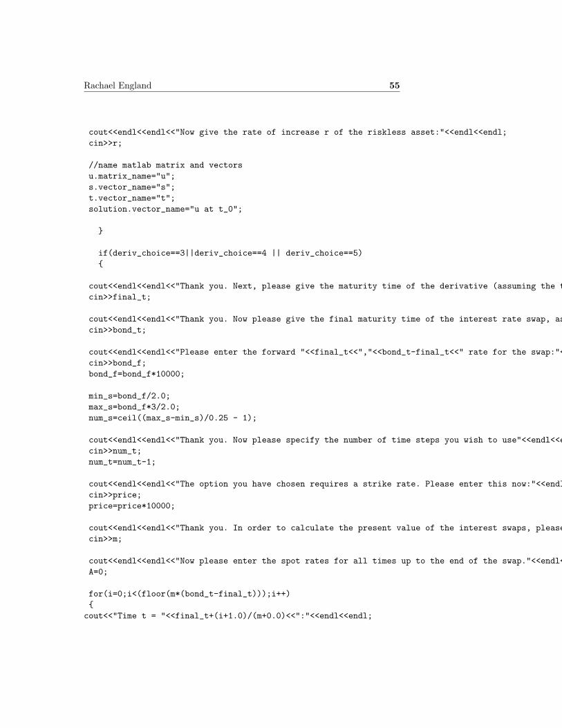
Rachael England 55
cout<<endl<<endl<<"Now give the rate of increase r of the riskless asset:"<<endl<<endl;cin>>r;
//name matlab matrix and vectorsu.matrix_name="u";s.vector_name="s";t.vector_name="t";solution.vector_name="u at t_0";
}
if(deriv_choice==3||deriv_choice==4 || deriv_choice==5){
cout<<endl<<endl<<"Thank you. Next, please give the maturity time of the derivative (assuming the time at the start is 0):"<<endl<<endl;cin>>final_t;
cout<<endl<<endl<<"Thank you. Now please give the final maturity time of the interest rate swap, assuming now to be time 0:"<<endl<<endl;cin>>bond_t;
cout<<endl<<endl<<"Please enter the forward "<<final_t<<","<<bond_t-final_t<<" rate for the swap:"<<endl<<endl;cin>>bond_f;bond_f=bond_f*10000;
min_s=bond_f/2.0;max_s=bond_f*3/2.0;num_s=ceil((max_s-min_s)/0.25 - 1);
cout<<endl<<endl<<"Thank you. Now please specify the number of time steps you wish to use"<<endl<<endl;cin>>num_t;num_t=num_t-1;
cout<<endl<<endl<<"The option you have chosen requires a strike rate. Please enter this now:"<<endl<<endl;cin>>price;price=price*10000;
cout<<endl<<endl<<"Thank you. In order to calculate the present value of the interest swaps, please enter the number of times per year the floating rate is paid:"<<endl<<endl;cin>>m;
cout<<endl<<endl<<"Now please enter the spot rates for all times up to the end of the swap."<<endl<<endl;A=0;
for(i=0;i<(floor(m*(bond_t-final_t)));i++){cout<<"Time t = "<<final_t+(i+1.0)/(m+0.0)<<":"<<endl<<endl;
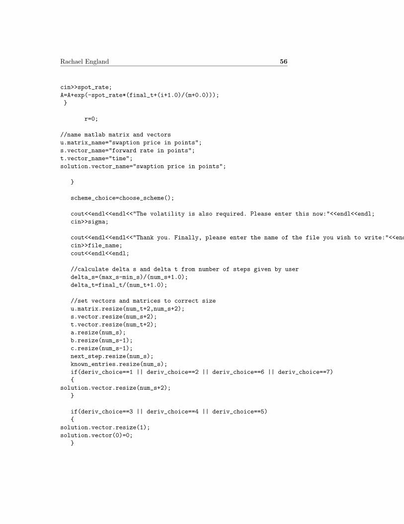
Rachael England 56
cin>>spot_rate;A=A+exp(-spot_rate*(final_t+(i+1.0)/(m+0.0)));}
r=0;
//name matlab matrix and vectorsu.matrix_name="swaption price in points";s.vector_name="forward rate in points";t.vector_name="time";solution.vector_name="swaption price in points";
}
scheme_choice=choose_scheme();
cout<<endl<<endl<<"The volatility is also required. Please enter this now:"<<endl<<endl;cin>>sigma;
cout<<endl<<endl<<"Thank you. Finally, please enter the name of the file you wish to write:"<<endl<<endl;cin>>file_name;cout<<endl<<endl;
//calculate delta s and delta t from number of steps given by userdelta_s=(max_s-min_s)/(num_s+1.0);delta_t=final_t/(num_t+1.0);
//set vectors and matrices to correct sizeu.matrix.resize(num_t+2,num_s+2);s.vector.resize(num_s+2);t.vector.resize(num_t+2);a.resize(num_s);b.resize(num_s-1);c.resize(num_s-1);next_step.resize(num_s);known_entries.resize(num_s);if(deriv_choice==1 || deriv_choice==2 || deriv_choice==6 || deriv_choice==7){
solution.vector.resize(num_s+2);}
if(deriv_choice==3 || deriv_choice==4 || deriv_choice==5){
solution.vector.resize(1);solution.vector(0)=0;
}

Rachael England 57
//loop for all s steps to fill in s valuesfor (i=0;i<s.vector.rows();i++)
{s.vector(i)=min_s+delta_s*i;
}
//loop for all t steps to fill in t valuesfor (i=0;i<t.vector.rows();i++){
t.vector(i)=delta_t*i;}
do{
//reset u matrix to 0u.matrix=0;
//insert boundary values using functionsu.matrix=boundary_s(r,t.vector,s.vector,deriv_choice,u.matrix,price);u.matrix=boundary_t(r,t.vector,s.vector,deriv_choice,u.matrix,price);
//fill in tridiagonal values for A matrix using a functionfill_matrix_A(a,b,c,sigma,s.vector,delta_t,delta_s,r,scheme_choice);
//loop through all time stepsfor (i=1;i<t.vector.rows();i++){//fill in entries for right hand side of equationknown_entries=fill_known(known_entries,u.matrix,i,sigma,s.vector,delta_t,delta_s,r,scheme_choice);
//solve tidiagonal equationnext_step=tridiag_solve(c,a,b,known_entries);
//indert solution back into u matrixfor (j=1;j<s.vector.rows()-1;j++){u.matrix(i,j)=next_step(j-1);}}
if(deriv_choice==3 || deriv_choice==4 || deriv_choice==5){for(i=0;i<s.vector.rows();i++){
Rachael England 58
if(s.vector(i)>bond_f && s.vector(i-1)<=bond_f){inter_above=u.matrix(t.vector.rows()-1,i);inter_below=u.matrix(t.vector.rows()-1,i-1);solution.vector(0)=solution.vector(0)+((inter_above-inter_below)/(s.vector(i)-s.vector(i-1))*(bond_f-s.vector(i-1))+inter_above)*A;break;}}}if(deriv_choice==5){straddle=true;deriv_choice=4;}else{straddle=false;}}while(straddle==true);
if(open_m(file_name)==true){//if file opens, write vectors to it and close file
if(deriv_choice==1 || deriv_choice==2 || deriv_choice==6 || deriv_choice==7){
writevector_m(s);for(i=0;i<s.vector.rows();i++){solution.vector(i)=u.matrix(t.vector.rows()-1,i);}
}
writevector_m(solution);
close_m();
//inform usercout<<"File has been written"<<endl;
}else{
//otherwise, inform user file opening has failedcout<<"Sorry; there was an error opening this file"<<endl;
}
//pause file to allow user to view, before returning an integer

Rachael England 59
system("PAUSE");
return 1;}
dissertation.h
//Header for outputting to file - Rachael England
//prevent looping error#ifndef DISSERTATION2_H#define DISSERTATION2_H
//include necessary libraries and header files#include "NSDE_maths.h"#include <string>
//define functionsint choose_deriv();int choose_scheme();Tmatrix boundary_s(double r,Tvector t,Tvector s,int choice, Tmatrix u,double E);Tmatrix boundary_t(double r,Tvector t,Tvector s,int choice, Tmatrix u, double E);void fill_matrix_A(Tvector& a,Tvector& b, Tvector& c,double sigma,Tvector s,double delta_t,double delta_s,double r,int choice);Tvector fill_known(Tvector d,Tmatrix u,int i,double sigma,Tvector s,double delta_t,double delta_s,double r,int choice);
#endif
dissertation.cpp
//include headers#include <iostream>#include "dissertation2.h"#include "NSDE_maths.h"
using namespace std;
int choose_deriv(){
int choice=0;
//list derivative choices and loop until user makes a valid choicedo
Rachael England 60
{cout<<endl<<endl<<"Now please choose one of the following derivatives to solve for:"<<endl<<endl;cout<<"1. European Call Option"<<endl;cout<<"2. European Put Option"<<endl;
cout<<"3. European Call Swaption"<<endl;cout<<"4. European Put Swaption"<<endl;cout<<"5. European Straddle Swaption"<<endl;cout<<"6. Digital Call Option"<<endl;cout<<"7. Digital Put Option"<<endl;
cin>>choice;}while (choice!=1 && choice!=2 && choice!=3 && choice!=4 && choice!=5 && choice!=6 && choice!=7);
//pass user’s choice back to main programreturn choice;
}
int choose_scheme(){
int choice=0;
//list scheme choices and loop until user makes a valid choicedo{
cout<<endl<<endl<<"Thank you. Now please choose which of the following schemes you wish to use:"<<endl<<endl;cout<<"1. Crank-Nicolson"<<endl;cout<<"2. Kenneth-Vetzal"<<endl;cout<<"3. Fully Implicit"<<endl;cout<<"4. Semi Implicit"<<endl;cout<<"5. Explicit 1"<<endl;cout<<"6. Explicit 2"<<endl;cin>>choice;
}while (choice!=1 && choice!=2 && choice!=3 && choice!=4 && choice!=5 && choice!=6);
//pass user’s choice back to main programreturn choice;
}
Tmatrix boundary_s( double r,Tvector t,Tvector s,int choice, Tmatrix u,double E){
int i;int end_s=s.rows()-1;
//loop through u for all time stepsfor (i=0;i<t.rows();i++){
//insert boundary conditions for minimum and maximum S values
Rachael England 61
//depending on the user’s choice of derivativeif (choice==1 || choice==3 || choice==5){
u(i,0)=0;u(i,end_s)=s(end_s)-E*exp(-r*t(i));
}if (choice==2 || choice==4){
u(i,0)=E*exp(-r*t(i))-s(0);u(i,end_s)=0;
}if(choice==6){
u(i,0)=0;u(i,end_s)=exp(-r*t(i));
}if(choice==7){
u(i,0)=exp(-r*t(i));u(i,end_s)=0;
}}
//pass resultant matrix back to main programreturn u;
}
Tmatrix boundary_t(double r,Tvector t,Tvector s,int choice, Tmatrix u, double E){
int i;
//loop through for all s stepsfor (i=0;i<s.rows();i++){
//insert initial condition at t=0 depending on//user’s choice of derivativeif(choice==1 || choice==3 || choice==5){
if (s(i)-E>0){
u(0,i)=s(i)-E;}else{
u(0,i)=0;}
Rachael England 62
}if(choice==2 || choice==4){
if (E-s(i)>0){
u(0,i)=E-s(i);}else{
u(0,i)=0;}
}if(choice==6){
if(s(i)-E>0){
u(0,i)=1;}else{
u(0,i)=0;}
}if(choice==7){
if(s(i)-E>0){
u(0,i)=0;}else{
u(0,i)=1;}
}}
//pass resultant matrix back to main programreturn u;
}
void fill_matrix_A(Tvector& a,Tvector& b,Tvector& c,double sigma,Tvector s,double delta_t,double delta_s,double r,int choice){
int i;double alpha;double beta;double gamma;

Rachael England 63
double theta_1;double theta_2;double theta_3;double theta_4;double theta_5;double theta_6;
//set theta values based on user’s choice of numerical schemeif (choice==1){
theta_1=0.5;theta_2=0.5;theta_3=0.5;theta_4=0.5;theta_5=0.5;theta_6=0.5;
}if (choice==2){
theta_1=1;theta_2=0;theta_3=1;theta_4=0;theta_5=0;theta_6=1;
}if (choice==3){
theta_1=1;theta_2=0;theta_3=1;theta_4=0;theta_5=1;theta_6=0;
}if (choice==4){
theta_1=1;theta_2=0;theta_3=0;theta_4=1;theta_5=1;theta_6=0;
}if (choice==5){

Rachael England 64
theta_1=0;theta_2=1;theta_3=0;theta_4=1;theta_5=0;theta_6=1;
}if (choice==6){
theta_1=0;theta_2=1;theta_3=0;theta_4=1;theta_5=1;theta_6=0;
}
//loop through all rows in the left hand side matrixfor (i=0;i<a.rows();i++){
//caluclate alpha, beta, and gamma for use in calculationsalpha=0.5*sigma*sigma*s(i+1)*s(i+1)*delta_t/(delta_s*delta_s);beta=0.5*r*s(i+1)*delta_t/delta_s;gamma=-r*delta_t;
//set a, b, and c values for the ith row of the matrix there//is no value for c in the first row, and no value for b in th//final row. Hence the c and b vectors are 1 unit smaller that a.if (i!=0 && i!=(a.rows()-1) ){
c(i-1)=-alpha*theta_1+beta*theta_3;a(i)=1+2*alpha*theta_1-gamma*theta_5;b(i)=-alpha*theta_1-beta*theta_3;
}else if(i==0){
a(i)=1+2*alpha*theta_1-gamma*theta_5;b(i)=-alpha*theta_1-beta*theta_3;
}else{
c(i-1)=-alpha*theta_1+beta*theta_3;a(i)=1+2*alpha*theta_1-gamma*theta_5;
}}//no need for return since a, b, and c were passed via pointers

Rachael England 65
}
Tvector fill_known(Tvector d,Tmatrix u,int i,double sigma,Tvector s,double delta_t,double delta_s,double r,int choice){
int j;double alpha;double beta;double gamma;double a;double b;double c;double theta_1;double theta_2;double theta_3;double theta_4;double theta_5;double theta_6;
//set theta values based on user’s choice of numerical schemeif (choice==1){
theta_1=0.5;theta_2=0.5;theta_3=0.5;theta_4=0.5;theta_5=0.5;theta_6=0.5;
}if (choice==2){
theta_1=1;theta_2=0;theta_3=1;theta_4=0;theta_5=0;theta_6=1;
}if (choice==3){
theta_1=1;theta_2=0;theta_3=1;theta_4=0;theta_5=1;theta_6=0;
}

Rachael England 66
if (choice==4){
theta_1=1;theta_2=0;theta_3=0;theta_4=1;theta_5=1;theta_6=0;
}if (choice==5){
theta_1=0;theta_2=1;theta_3=0;theta_4=1;theta_5=0;theta_6=1;
}if (choice==6){
theta_1=0;theta_2=1;theta_3=0;theta_4=1;theta_5=1;theta_6=0;
}
//loop through all rows in the right hand side vectorfor (j=0;j<d.rows();j++){
//calculate alpha beta and gamma for use in calculating vector valuesalpha=0.5*sigma*sigma*s(j+1)*s(j+1)*delta_t/(delta_s*delta_s);beta=0.5*r*s(j+1)*delta_t/delta_s;gamma=-r*delta_t;
//use alpha beta and gamma to calculate the entries for Bc=alpha*theta_2-beta*theta_4;a=1-2*alpha*theta_2+gamma*theta_6;b=alpha*theta_2+beta*theta_4;
//use a b and c to work out right hand side through equation//B u_j + boundary conditions for first and final rowsif (j!=0 && j!=(d.rows()-1) ){
d(j)=c*u(i-1,j)+a*u(i-1,j+1)+b*u(i-1,j+2);
Rachael England 67
}else if(j==0){
d(j)=c*u(i-1,j)+a*u(i-1,j+1)+b*u(i-1,j+2)+(alpha*theta_1-beta*theta_3)*u(i,j);}else{
d(j)=c*u(i-1,j)+a*u(i-1,j+1)+b*u(i-1,j+2)+(alpha*theta_1+beta*theta_3)*u(i,j+2);}
}return d;
}
NSDE_maths.h
//Maths header file - Rachael England
//Prevent looping error#ifndef NSDE_MATHS_H#define NSDE_MATHS_H
//include all libraries needed#include <cmath>#include <complex>#include <blitz\array.h>
//Add in namespace blitzusing namespace blitz;
//define matrix and vector typestypedef Array <double,1> Tvector;typedef Array <double,2> Tmatrix;
Tvector matrixXvector(Tmatrix A, Tvector b);Tmatrix matrixXmatrix(Tmatrix A, Tmatrix B);Tvector tridiag_solve(Tvector a,Tvector b,Tvector c,Tvector r);Tmatrix tridiag_solve_matrix(Tvector a,Tvector b,Tvector c,Tmatrix r);Tvector gauss_seidel(Tmatrix A, Tvector b);double max_d(double a, double b);
#endif
NSDE_maths.cpp

Rachael England 68
//Mathematical Functions - Rachael England
//include headers#include <iostream>#include "NSDE_maths.h"
using namespace std;
Tvector matrixXvector(Tmatrix A, Tvector b){
int i;int j;
Tvector answer;
answer.resize(A.rows());//multiply the matrix by the vector if possibleif (A.cols()==b.rows()){
//loop for all rows of the resultant vectorfor (i=0; i<A.rows(); i++){
j=0;answer(i)=0;
for (j=0; j<A.cols(); j++){
//using the formula for multiplying a matrix with a vectoranswer(i)=answer(i)+A(i,j)*b(j);
}}
}else{
cout<<"Sorry, it is not possible to multiply the matrix by the vector"<<endl<<endl;system("PAUSE");}
return answer;}
Tmatrix matrixXmatrix(Tmatrix A, Tmatrix B){
int i;int j;

Rachael England 69
Tmatrix solution;Tvector x;
solution.resize(B.rows(),B.cols());x.resize(B.rows());
for(i=0;i<B.cols();i++){
for(j=0;j<B.rows();j++){
x(j)=B(j,i);}x=matrixXvector(A,x);for(j=0;j<B.rows();j++){
solution(j,i)=x(j);}}return solution;
}
Tvector tridiag_solve(Tvector a,Tvector b,Tvector c,Tvector r){
int i;int n;Tvector w;Tvector alpha;Tvector beta;Tvector gamma;Tvector u;
n=r.rows();
w.resize(n);alpha.resize(n);beta.resize(n);gamma.resize(n);u.resize(n);
//test correct number of rows for solver to workif(b.rows()==a.rows()+1 && b.rows()==c.rows()+1 && b.rows()==r.rows()){
//use new vectors to store diagonals for lower and upper triangular factorisation//amd use w vector to store forward substitution stagebeta(0) = b(0);

Rachael England 70
gamma(0) = c(0);w(0) = r(0);for(i=1;i<n;i++){
alpha(i) = a(i-1)/beta(i-1);beta(i) = b(i) - alpha(i)*gamma(i-1);gamma(i) = c(i);w(i) = r(i) - alpha(i)*w(i-1);
}
//backwards substitution calculated and stored in yu(n-1)=w(n-1)/beta(n-1);for(i=n-2;i>=0;i--){
u(i)= (w(i)-gamma(i)*u(i+1))/beta(i);}
}else{
cout<<"Sorry, it is not possible to solve this as the number of diagonal entries do not match.";system("PAUSE");}
//solution in y passed back to main functionreturn u;
}
Tmatrix tridiag_solve_matrix(Tvector a,Tvector b,Tvector c,Tmatrix r){
int i;int j;Tmatrix solution;Tvector x;
solution.resize(r.rows(),r.cols());x.resize(r.rows());
for(i=0;i<r.cols();i++){
for(j=0;j<r.rows();j++){
x(j)=r(j,i);}x=tridiag_solve(a,b,c,x);for(j=0;j<r.rows();j++){
Rachael England 71
solution(j,i)=x(j);}}return solution;
}
Tvector gauss_seidel(Tmatrix A, Tvector b){
int j;int k;Tvector x_new;Tvector x_old;double sum1;double sum2;double check;
//set x to correct sizex_old.resize(b.rows());x_new.resize(b.rows());x_old=0;
//check columns of A matches with rows of bif(A.cols()==x_new.rows()){
//loopm until within tolerance leveldo
{//loop through all rows
for(j=0;j<b.rows();j++){
sum1=0;sum2=0;
//loop through rows to get first sum, i.e. sum from k=0 to j-1 of A(j,k)x_new(k)for(k=0;k<j;k++)
{sum1=sum1+(A(j,k)*x_new(k));
}
//loop through for second sum; i.e. sum from k=j+1 to final row of A(j,k)x_old(k)for(k=j+1;k<b.rows();k++){
sum2=sum2+(A(j,k)*x_old(k));}
//perform calculation: x(j)=1/A(j,j)[b(j) - sum1 - sum2]

Rachael England 72
x_new(j)=(1.0/A(j,j))*(b(j) - sum1-sum2);}
//check error//reset check to 0
check=0;for(j=0;j<b.rows();j++){
//add |new x - old x| for row j onto checkcheck=check+fabs(x_new(j)-x_old(j));}
//set old x for next loopx_old=x_new;
//loop until within tolerance level}while (check>0.00001*b.rows());
}else{
cout<<"Sorry; it is not possible to solve this matrix equation";system("PAUSE");}
return x_new;}
double max_d(double a, double b){double solution;
solution=0.5*(fabs(a-b) + a + b);
return solution;}
NSDE_output.h
//Header for outputting to file - Rachael England
//prevent looping error#ifndef NSDE_OUTPUT_H#define NSDE_OUTPUT_H
Rachael England 73
//include necessary libraries and header files#include "NSDE_maths.h"#include <fstream>#include <string>
//define matlab matrix and vector structurestypedef struct{string matrix_name;Tmatrix matrix;
} TmatlabMatrix;
typedef struct{string vector_name;Tvector vector;} TmatlabVector;
//define output functions for NSDE_output.cppbool open_m (string file_name);void close_m (void);void writevector_m (TmatlabVector mat_vector);void writematrix_m (TmatlabMatrix mat_matrix);void plot_m (TmatlabVector x1, TmatlabVector x2);void plot2_m (TmatlabVector x1, TmatlabVector x2, TmatlabVector x3);void plot3D_m (TmatlabVector x1, TmatlabVector x2, TmatlabMatrix u);void plot_function(string function_str, double a, double b);void output_string(string string_value);
#endif
NSDE_output.cpp
//Outputting to file - Rachael England
//include headers#include <iostream>#include "NSDE_output.h"#include "NSDE_maths.h"
using namespace std;
//define global variable

Rachael England 74
ofstream fout;
bool open_m (string file_name){
//open file and return boolean depending on whether operation succeededfout.open (file_name.c_str ());return fout.good ();
}
void close_m (void){
//if file opened,close fileif(fout.good()){fout.close ();}
}
void writevector_m (TmatlabVector mat_vector){
//define variablesint i;
//write to file as ’name = [’fout<<mat_vector.vector_name;fout<<" = [";
for (i=0; i<mat_vector.vector.rows(); i++){
//for each value in the vector, add onto the file ’value’fout<<mat_vector.vector(i);
//if it’s the last value, put ’];’ on the file, else add ’, ’if (i!=mat_vector.vector.rows()-1){
fout<<", ";}else{
fout<<"];";}
}
//final output looks like: ’name = [ value, value, value, ... ];’; write this to the file//add a new line for matlab to seperate out commandsfout<<endl;
Rachael England 75
}
void writematrix_m (TmatlabMatrix mat_matrix){
//define variablesint i,j;
//write to file as ’name = [’fout<<mat_matrix.matrix_name;fout<<" = [";
for (i=0; i<mat_matrix.matrix.rows();i++){
//add onto ’;’ for the start of each new row in the matrixif (i!=0){
fout<<";"<<endl;}
for (j=0; j<mat_matrix.matrix.cols();j++){
//for each value in the row, add onto the file ’value’fout<<mat_matrix.matrix(i,j);
//if it’s not the last value in the row, add ’, ’if (j!=mat_matrix.matrix.cols()-1){
fout<<", ";}
}}
//finish off the string with ’];’fout<<"];";
//the final output looks like://’name = [ value, value, value, ... ;value, value, value, ... ; ... ];’//add line to inform matlab of new commandfout<<endl;
}
void plot_m (TmatlabVector x1, TmatlabVector x2){
//output Matlab instructions for plotting graphfout<<"figure; plot ("<<x1.vector_name<<","<<x2.vector_name<<");"<<endl;
}
Rachael England 76
void plot2_m (TmatlabVector x1, TmatlabVector x2, TmatlabVector x3){
//output Matlab instructions for plotting graph with extra variablefout<<"figure; plot ("<<x1.vector_name<<","<<x2.vector_name<<","<<x1.vector_name<<","<<x3.vector_name<<");"<<endl;
}
void plot3D_m (TmatlabVector x1, TmatlabVector x2, TmatlabMatrix u){
//output Matlab instructions for plotting 3D graph of a matrixfout<<"figure; surf("<<x1.vector_name<<", "<<x2.vector_name<<","<<u.matrix_name<<");"<<endl;
}
void plot_function(string function_str, double a, double b){
//output Matlab instructions for plotting specified function between x=a and x=bfout<<"y=linspace("<<a<<","<<b<<");"<<endl;fout<<"plot(y,"<<function_str<<");"<<endl;
}
void output_string(string string_value){
//output string to filefout<<string_value<<endl;
}
Coding for Heston Program
Hston_main.cpp
//Rachael England: Program for numerical solution of the Heston equation
//include necessary headers and namespace#include <iostream>#include "NSDE_maths.h"#include "NSDE_output.h"#include "heston.h"
using namespace std;
int main (void){//define variables

Rachael England 77
int j;int k;int num_s;int num_v;int num_t;double delta_s;double delta_v;double delta_t;double t_end;double s_min;double s_max;double v_min;double v_max;double bond_f;double bond_t;double rho;double sigma;double r;double K;double theta;double E;double E2;double A;double inter_above;double inter_below;int scheme;int deriv;TmatlabVector s;TmatlabVector v;Tvector t;TmatlabMatrix u;Tmatrix u_old;TmatlabVector solution;Tmatrix rhs;Tmatrix a;Tmatrix b;Tmatrix c;Tmatrix d;Tmatrix e;Tmatrix f;Tmatrix g;Tmatrix h;Tmatrix l;string file_name;
//ask user for input

Rachael England 78
cout<<"This program uses a numerical method to solve the ";cout<<"Heston equation."<<endl<<endl;
deriv=choose_deriv();
//required input varies depending on choice of derivativeif(deriv==1 || deriv==2 || deriv==6){cout<<"In order to solve numerically, a suitably small and a suitably large value of the ";cout<<"asset price must be used to mimick boundary conditions as the asset price approaches 0 or infinity."<<endl;cout<<"Please enter a suitably small value:"<<endl<<endl;cin>>s_min;
cout<<endl<<endl<<"Thank you. Now please enter a suitably large value:"<<endl<<endl;cin>>s_max;
cout<<endl<<endl<<"Similar conditions are required for the volatility."<<endl;cout<<"Please enter a suitably small value:"<<endl<<endl;
cin>>v_min;
cout<<endl<<endl<<"Thank you. Now please enter a suitably large value:"<<endl<<endl;cin>>v_max;
cout<<endl<<endl<<"Thank you. Next, please give the final time (assuming the time at the start is 0):"<<endl<<endl;cin>>t_end;
cout<<endl<<endl<<"Please specify the number of asset price steps you wish to use"<<endl<<endl;cin>>num_s;num_s=num_s-1;
cout<<endl<<endl<<"Thank you. Please enter a value for theta (the average volatility):"<<endl<<endl;cin>>theta;
cout<<endl<<endl<<"Please specify the number of volatility steps you wish to use"<<endl<<endl;cin>>num_v;num_v=num_v-1;
cout<<endl<<endl<<"Please specify the number of time steps you wish to use"<<endl<<endl;cin>>num_t;num_t=num_t-1;
if(deriv==6){cout<<endl<<endl<<"The derivative you have chosen requies two strike prices. Firstly, please enter the strike price E2 below which the payof is zero:"<<endl<<endl;cin>>E2;

Rachael England 79
cout<<endl<<endl<<"Thank you. Now please enter the srike price E1, used to calculate the payoff (i.e. S - E1):"<<endl<<endl;cin>>E;}else{cout<<endl<<endl<<"The option you have chosen requires a strike price. Please enter this now:"<<endl<<endl;cin>>E;}
cout<<endl<<endl<<"Now give the rate of increase r of the riskless asset:"<<endl<<endl;cin>>r;
u.matrix_name="Price of Derivative U at Initial Time";s.vector_name="Asset Price S";v.vector_name="Volatility v";
}
if(deriv==3||deriv==4 || deriv==5){
cout<<endl<<endl<<"Thank you. Next, please give the maturity time of the derivative (assuming the time at the start is 0):"<<endl<<endl;cin>>t_end;
cout<<endl<<endl<<"Thank you. Now please give the final maturity time of the interest rate swap, assuming now to be time 0:"<<endl<<endl;cin>>bond_t;
cout<<endl<<endl<<"Please enter the forward "<<t_end<<","<<bond_t-t_end<<" rate for the swap:"<<endl<<endl;cin>>bond_f;bond_f=bond_f*10000;
s_min=bond_f*3.0/4.0;s_max=bond_f*5.0/4.0;
num_s=ceil((s_max-s_min)/0.5 - 1);
cout<<endl<<endl<<"Thank you. Now please specify the number of time steps you wish to use"<<endl<<endl;cin>>num_t;num_t=num_t-1;
cout<<endl<<endl<<"The option you have chosen requires a strike rate. Please enter this now:"<<endl<<endl;cin>>E;E=E*10000;
cout<<endl<<endl<<"Thank you. Please enter a value for theta (the average volatility):"<<endl<<endl;cin>>theta;
Rachael England 80
v_min=theta*1.0/2.0;v_max=theta*3.0/2.0;
num_v=ceil((v_max-v_min)/0.005 - 1);
cout<<endl<<endl<<"Thank you. In order to calculate the present value of the interest swaps, please enter the number of times per year the floating rate is paid:"<<endl<<endl;cin>>m;
cout<<endl<<endl<<"Now please enter the spot rates for all times up to the end of the swap."<<endl<<endl;A=0;
for(i=0;i<(floor(m*(bond_t-final_t)));i++){cout<<"Time t = "<<final_t+(i+1.0)/(m+0.0)<<":"<<endl<<endl;cin>>spot_rate;A=A+exp(-spot_rate*(final_t+(i+1.0)/(m+0.0)));}A=A/(m+0.0);
r=0;
//name matlab matrix and vectors
u.matrix_name="Price of Swaption at Initial Time";s.vector_name="Forward Rate";v.vector_name="Volatility";solution.vector_name="solution";
solution.vector.resize(num_v+2);}
scheme=choose_scheme();
cout<<endl<<endl<<"The value of sigma is also required. Please enter this now:"<<endl<<endl;cin>>sigma;
cout<<endl<<endl<<"Please enter a value for rho:"<<endl<<endl;cin>>rho;
cout<<endl<<endl<<"Please enter a value for k:"<<endl<<endl;cin>>K;
cout<<endl<<endl<<"Thank you. Finally, please enter the name of the file you wish to write:"<<endl<<endl;cin>>file_name;cout<<endl<<endl;
Rachael England 81
//calculate step sizes and resize matrices and ectorsdelta_s=(s_max-s_min)/(num_s+1.0);delta_v=(v_max-v_min)/(num_v+1.0);delta_t=t_end/(num_t+1.0);
s.vector.resize(num_s+2);v.vector.resize(num_v+2);t.resize(num_t+2);u.matrix.resize(num_s+2,num_v+2);u_old.resize(num_s+2,num_v+2);a.resize(num_s,num_v+2);b.resize(num_s,num_v+2);c.resize(num_s,num_v+2);d.resize(num_s,num_v+2);e.resize(num_s,num_v+2);f.resize(num_s,num_v+2);g.resize(num_s,num_v+2);h.resize(num_s,num_v+2);l.resize(num_s,num_v+2);rhs.resize(num_s,num_v+2);
//fill in discrete values for S, v, and taufill_grid(s.vector,s_min,delta_s);fill_grid(v.vector,v_min,delta_v);fill_grid(t,0,delta_t);
//loop through all time stepsfor(j=0;j<t.rows();j++){if(j==0){//fil in initial values if j=0t_boundary(r,s.vector,deriv,u.matrix,E,E2);}else{//fill in boundary valuess_boundary(r,t,s.vector,deriv,u.matrix,E,j);
//enter values into diagonals of Adefine_A(a,b,c,d,e,f,g,h,l,s.vector,v.vector,delta_s,delta_v,delta_t,rho,sigma,r,K,theta,j,scheme);
//enter vlues into right hand side vectordefine_rhs(u_old,u.matrix,a,b,c,d,e,f,g,h,l,rhs,s.vector,v.vector,delta_s,delta_v,delta_t,rho,sigma,r,K,theta,j,scheme);
Rachael England 82
//solve matrix equation using Gauss-Seidel iterationsolve_gs(a,b,c,d,e,f,g,h,l,u.matrix,rhs);}//put values into u_old matrix for use in next time stepu_old=u.matrix;}
if(open_m(file_name)==true){
//if file opens, write vectors to it and close filewritevector_m(v);
if(deriv==1 || deriv==2 || deriv==6){
writevector_m(s);writematrix_m(u);
}if(deriv==3 || deriv==4 || deriv==5){
for(j=1;j<s.vector.rows();j++){if(s.vector(j)>bond_f && s.vector(j-1)<=bond_f){for(k=0;k<v.vector.rows();k++){inter_above=u.matrix(j,k);inter_below=u.matrix(j-1,k);solution.vector(k)=((inter_above-inter_below)/(s.vector(j)-s.vector(j-1))*(bond_f-s.vector(j-1))+inter_above)*A;}}}writevector_m(solution);
}
close_m();
//inform usercout<<"File has been written"<<endl;
}else{
//otherwise, inform user file opening has failedcout<<"Sorry; there was an error opening this file"<<endl;
}
//pause file to allow user to view, before returning an integersystem("PAUSE");

Rachael England 83
return 1;}
Heston.h
//prevent looping error#ifndef HESTON2_H#define HESTON2_H
//include necessary libraries and header files#include "NSDE_maths.h"#include <fstream>#include <string>
//define functionsint choose_scheme(void);int choose_deriv(void);void fill_grid(Tvector& x,double min,double delta_x);void s_boundary(double r,Tvector& t,Tvector& s,int choice, Tmatrix& u,double E,int j);void t_boundary(double r,Tvector& s,int choice, Tmatrix& u, double E,double E2);void define_A(Tmatrix& a, Tmatrix& b, Tmatrix& c, Tmatrix& d, Tmatrix& e, Tmatrix& f, Tmatrix& g, Tmatrix& h, Tmatrix& l, Tvector& s, Tvector& v, double delta_s, double delta_v, double delta_t, double rho, double sigma, double r, double K, double theta, int j, int choice);void define_rhs(Tmatrix& u_old, Tmatrix& u, Tmatrix& a, Tmatrix& b, Tmatrix& c, Tmatrix& d, Tmatrix& e, Tmatrix& f, Tmatrix& g, Tmatrix& h, Tmatrix& l, Tmatrix& rhs, Tvector& s, Tvector& v, double delta_s, double delta_v, double delta_t, double rho, double sigma, double r, double K, double theta, int j, int choice);void solve_gs(Tmatrix& a,Tmatrix& b,Tmatrix& c,Tmatrix& d,Tmatrix& e,Tmatrix& f,Tmatrix& g,Tmatrix& h,Tmatrix& l,Tmatrix& u,Tmatrix& rhs);double lambda(double s, double v, double t);
#endif
Heston.cpp
//include headers#include <iostream>#include "heston2.h"#include "NSDE_maths.h"
using namespace std;
int choose_deriv(){int choice=0;
//list derivative choices and loop until user makes a valid choicedo{
Rachael England 84
cout<<endl<<endl<<"Now please choose one of the following derivatives to solve for:"<<endl<<endl;cout<<"1. Call Option"<<endl;cout<<"2. Put Option"<<endl;cout<<"3. European Call Swaption"<<endl;cout<<"4. European Put Swaption"<<endl;cout<<"5. European Straddle Swaption"<<endl;cout<<"6. Knock-in Cap"<<endl;cin>>choice;}while (choice!=1 && choice!=2 && choice!=3 && choice!=4 && choice!=5 && choice!=6);
//pass user’s choice back to main programreturn choice;}
int choose_scheme(){
int choice=0;
//list scheme choices and loop until user makes a valid choicedo{
cout<<endl<<endl<<"Thank you. Now please choose which of the following schemes you wish to use:"<<endl<<endl;cout<<"1. Crank-Nicolson"<<endl;cout<<"2. Kenneth-Vetzal"<<endl;cout<<"3. Fully Implicit"<<endl;cout<<"4. Semi Implicit"<<endl;cout<<"5. Explicit 1"<<endl;cout<<"6. Explicit 2"<<endl;cin>>choice;
}while (choice!=1 && choice!=2 && choice!=3 && choice!=4 && choice!=5 && choice!=6);
//pass user’s choice back to main programreturn choice;
}
void fill_grid(Tvector& x,double min,double delta_x){int i;
//loop through vector and fill in discret value for each stepfor(i=0;i<x.rows();i++){
x(i)=min+i*delta_x;}}
Rachael England 85
void s_boundary( double r,Tvector& t,Tvector& s,int choice, Tmatrix& u,double E,int j){
int k;int end_s=s.rows()-1;
//loop through u for all v stepsfor (k=0;k<u.cols();k++){
//insert boundary conditions for minimum and maximum s values//depending on the user’s choice of derivativeif (choice==1 || choice==3 || choice==6){
u(0,k)=0;u(end_s,k)=s(end_s)-E*exp(-r*t(j));
}if (choice==2 || choice==4){
u(0,k)=E*exp(-r*t(j))-s(0);u(end_s,k)=0;
}if (choice==5){
u(0,k)=E*exp(-r*t(j))-s(0);u(end_s,k)=s(end_s)-E*exp(-r*t(j));
}}
}
void t_boundary(double r,Tvector& s,int choice, Tmatrix& u, double E, double E2){
int i;int k;
//loop through for all s stepsfor (i=0;i<s.rows();i++){
//loop through for all v stepsfor(k=0;k<u.cols();k++)
{//insert initial condition at t=0 depending on
//user’s choice of derivativeif(choice==1 || choice==3){
if (s(i)-E>0){
u(i,k)=s(i)-E;

Rachael England 86
}else{
u(i,k)=0;}
}if(choice==2 || choice==4){
if (E-s(i)>0){
u(i,k)=E-s(i);}else{
u(i,k)=0;}
}if(choice==5){
if (E-s(i)>0){
u(i,k)=E-s(i);}else{
u(i,k)=s(i)-E;}
}if(choice==6){
if(s(i)>E2){u(i,k)=s(i)-E;}else{u(i,k)=0;}}
}}
}
void define_A(Tmatrix& a, Tmatrix& b, Tmatrix& c, Tmatrix& d, Tmatrix& e, Tmatrix& f, Tmatrix& g, Tmatrix& h, Tmatrix& l, Tvector& s, Tvector& v, double delta_s, double delta_v, double delta_t, double rho, double sigma, double r, double K, double theta, int j, int choice){int i;

Rachael England 87
int k;double alpha;double beta;double gamma;double zeta;double eta;double mu=-r*delta_t;double theta_1;double theta_2;double theta_3;double theta_4;double theta_5;double theta_6;double theta_7;double theta_8;double theta_9;double theta_10;double theta_11;double theta_12;
//set theta values based on user’s choice of numerical schemeif (choice==1){
theta_1=0.5;theta_2=0.5;theta_3=0.5;theta_4=0.5;theta_5=0.5;theta_6=0.5;
theta_7=0.5;theta_8=0.5;theta_9=0.5;theta_10=0.5;theta_11=0.5;theta_12=0.5;}if (choice==2){
theta_1=1;theta_2=0;theta_3=1;theta_4=0;
theta_5=1;theta_6=0;theta_7=1;theta_8=0;
Rachael England 88
theta_9=1;theta_10=0;
theta_11=0;theta_12=1;
}if (choice==3){
theta_1=1;theta_2=0;theta_3=1;theta_4=0;theta_5=1;theta_6=0;
theta_7=1;theta_8=0;theta_9=1;theta_10=0;theta_11=1;theta_12=0;}if (choice==4){
theta_1=1;theta_2=0;theta_3=1;
theta_4=0;theta_5=1;theta_6=0;theta_7=0;theta_8=1;theta_9=0;
theta_10=1;theta_11=1;theta_12=0;
}if (choice==5){
theta_1=0;theta_2=1;theta_3=0;theta_4=1;theta_5=0;theta_6=1;
theta_7=0;theta_8=1;theta_9=0;
Rachael England 89
theta_10=1;theta_11=0;theta_12=1;}if (choice==6){
theta_1=0;theta_2=1;theta_3=0;theta_4=1;
theta_5=0;theta_6=1;theta_7=0;theta_8=1;theta_9=0;theta_10=1;
theta_11=1;theta_12=0;
}
//loop through all S and v valuesfor(i=0;i<a.rows();i++){for(k=0;k<a.cols();k++){//calculate alpha, etc.alpha=0.5*v(k)*s(i+1)*s(i+1)*delta_t/(delta_s*delta_s);beta=0.25*rho*sigma*v(k)*s(i+1)*delta_t/(delta_v*delta_s);gamma=0.5*sigma*sigma*v(k)*delta_t/(delta_v*delta_v);zeta=0.5*r*s(i+1)*delta_t/delta_s;eta=0.5*(K*(theta-v(k))-lambda(s(i+1),v(k),delta_t*j))*delta_t/delta_v;
//calculate a, b, etc. using alpha, etc.a(i,k)=-beta*theta_3;b(i,k)=-alpha*theta_1+zeta*theta_7;c(i,k)=beta*theta_3;d(i,k)=-gamma*theta_5+eta*theta_9;e(i,k)=1+2*alpha*theta_1+2*gamma*theta_5-mu*theta_11;f(i,k)=-gamma*theta_5-eta*theta_9;g(i,k)=beta*theta_3;h(i,k)=-alpha*theta_1-zeta*theta_7;l(i,k)=-beta*theta_3;}}}

Rachael England 90
void define_rhs(Tmatrix& u_old, Tmatrix& u, Tmatrix& a, Tmatrix& b, Tmatrix& c, Tmatrix& d, Tmatrix& e, Tmatrix& f, Tmatrix& g, Tmatrix& h, Tmatrix& l, Tmatrix& rhs, Tvector& s, Tvector& v, double delta_s, double delta_v, double delta_t, double rho, double sigma, double r, double K, double theta, int j, int choice){int i;int k;double alpha;double beta;double gamma;double zeta;double eta;double mu=-r*delta_t;double a_;double b_;double c_;double d_;double e_;double f_;double g_;double h_;double l_;double theta_1;double theta_2;double theta_3;double theta_4;double theta_5;double theta_6;double theta_7;double theta_8;double theta_9;double theta_10;double theta_11;double theta_12;
//set theta values based on user’s choice of numerical schemeif (choice==1){
theta_1=0.5;theta_2=0.5;theta_3=0.5;theta_4=0.5;theta_5=0.5;theta_6=0.5;
theta_7=0.5;theta_8=0.5;theta_9=0.5;theta_10=0.5;theta_11=0.5;

Rachael England 91
theta_12=0.5;}if (choice==2){
theta_1=1;theta_2=0;theta_3=1;theta_4=0;
theta_5=1;theta_6=0;theta_7=1;theta_8=0;theta_9=1;theta_10=0;
theta_11=0;theta_12=1;
}if (choice==3){
theta_1=1;theta_2=0;theta_3=1;theta_4=0;theta_5=1;theta_6=0;
theta_7=1;theta_8=0;theta_9=1;theta_10=0;theta_11=1;theta_12=0;}if (choice==4){
theta_1=1;theta_2=0;theta_3=1;
theta_4=0;theta_5=1;theta_6=0;theta_7=0;theta_8=1;theta_9=0;
theta_10=1;theta_11=1;theta_12=0;
Rachael England 92
}if (choice==5){
theta_1=0;theta_2=1;theta_3=0;theta_4=1;theta_5=0;theta_6=1;
theta_7=0;theta_8=1;theta_9=0;theta_10=1;theta_11=0;theta_12=1;}if (choice==6){
theta_1=0;theta_2=1;theta_3=0;theta_4=1;
theta_5=0;theta_6=1;theta_7=0;theta_8=1;theta_9=0;theta_10=1;
theta_11=1;theta_12=0;
}
//loop through all S and v valuesfor(i=0;i<a.rows();i++){for(k=0;k<a.cols();k++){//calculate alpha, beta, etc.alpha=0.5*v(k)*s(i+1)*s(i+1)*delta_t/(delta_s*delta_s);beta=0.25*rho*sigma*v(k)*s(i+1)*delta_t/(delta_s*delta_v);gamma=0.5*sigma*sigma*v(k)*delta_t/(delta_v*delta_v);zeta=0.5*r*s(i+1)*delta_t/delta_s;eta=0.5*(K*(theta-v(k))-lambda(s(i+1),v(k),delta_t*j))*delta_t/delta_v;
//use alpha, etc. to calculate a_, b_, etc.a_=beta*theta_4;

Rachael England 93
b_=alpha*theta_2-zeta*theta_8;c_=-beta*theta_4;d_=gamma*theta_6-eta*theta_10;e_=1-2*alpha*theta_2-2*gamma*theta_6+mu*theta_12;f_=gamma*theta_6+eta*theta_10;g_=-beta*theta_4;h_=alpha*theta_2+zeta*theta_8;l_=beta*theta_4;
//calculate entry for right hand side vectorif(k==0){rhs(i,k)=a_*u_old(i,k+1)+b_*u_old(i,k)+c_*u_old(i,k+1)+d_*u_old(i+1,k+1)+e_*u_old(i+1,k)+f_*u_old(i+1,k+1)+g_*u_old(i+2,k+1)+h_*u_old(i+2,k)+l_*u_old(i+2,k+1);if(i==0){rhs(i,k)=rhs(i,k)-a(i,k)*u(i,k+1)-b(i,k)*u(i,k)-c(i,k)*u(i,k+1);}else if(i==e.rows()-1){rhs(i,k)=rhs(i,k)-g(i,k)*u(i+2,k+1)-h(i,k)*u(i+2,k)-l(i,k)*u(i+2,k+1);}}else if(k==e.cols()-1){rhs(i,k)=a_*u_old(i,k-1)+b_*u_old(i,k)+c_*u_old(i,k-1)+d_*u_old(i+1,k-1)+e_*u_old(i+1,k)+f_*u_old(i+1,k-1)+g_*u_old(i+2,k-1)+h_*u_old(i+2,k)+l_*u_old(i+2,k-1);if(i==0){rhs(i,k)=rhs(i,k)-a(i,k)*u(i,k-1)-b(i,k)*u(i,k)-c(i,k)*u(i,k-1);}else if(i==e.rows()-1){rhs(i,k)=rhs(i,k)-g(i,k)*u(i+2,k-1)-h(i,k)*u(i+2,k)-l(i,k)*u(i+2,k-1);}}else{rhs(i,k)=a_*u_old(i,k-1)+b_*u_old(i,k)+c_*u_old(i,k+1)+d_*u_old(i+1,k-1)+e_*u_old(i+1,k)+f_*u_old(i+1,k+1)+g_*u_old(i+2,k-1)+h_*u_old(i+2,k)+l_*u_old(i+2,k+1);if(i==0){rhs(i,k)=rhs(i,k)-a(i,k)*u(i,k-1)-b(i,k)*u(i,k)-c(i,k)*u(i,k+1);}else if(i==e.rows()-1){rhs(i,k)=rhs(i,k)-g(i,k)*u(i+2,k-1)-h(i,k)*u(i+2,k)-l(i,k)*u(i+2,k+1);}}
Rachael England 94
}}}
void solve_gs(Tmatrix& a,Tmatrix& b,Tmatrix& c,Tmatrix& d,Tmatrix& e,Tmatrix& f,Tmatrix& g,Tmatrix& h,Tmatrix& l,Tmatrix& u,Tmatrix& rhs){int i;int k;Tmatrix x;double x_old;double check;
x.resize(rhs.rows(),rhs.cols());x=0;
//loop through iterations until error is within tolerancedo{//reset error check variable to 0check=0;
for(i=0;i<x.rows();i++){for(k=0;k<x.cols();k++){x_old=x(i,k);
//calculate next iteration based on Gauss-Seidel formulaif(k==0){if(i==0){x(i,k)=(1.0/e(i,k))*(rhs(i,k)-((f(i,k)+d(i,k))*x(i,k+1) + h(i,k)*x(i+1,k) + (l(i,k)+g(i,k))*x(i+1,k+1)));}else if(i==x.rows()-1){x(i,k)=(1.0/e(i,k))*(rhs(i,k)-(b(i,k)*x(i-1,k)+(c(i,k)+a(i,k))*x(i-1,k+1)+(f(i,k)+d(i,k))*x(i,k+1)));}else{x(i,k)=(1.0/e(i,k))*(rhs(i,k)-(b(i,k)*x(i-1,k)+h(i,k)*x(i+1,k)+(c(i,k)+a(i,k))*x(i-1,k+1)+(f(i,k)+d(i,k))*x(i,k+1)+(l(i,k)+g(i,k))*x(i+1,k+1)));}}else if (k==x.cols()-1){if(i==0)

Rachael England 95
{x(i,k)=(1.0/e(i,k))*(rhs(i,k)-((f(i,k)+d(i,k))*x(i,k-1) + h(i,k)*x(i+1,k) + (l(i,k)+g(i,k))*x(i+1,k-1)));}else if(i==x.rows()-1){x(i,k)=(1.0/e(i,k))*(rhs(i,k)-(b(i,k)*x(i-1,k)+(c(i,k)+a(i,k))*x(i-1,k-1)+(f(i,k)+d(i,k))*x(i,k-1)));}else{x(i,k)=(1.0/e(i,k))*(rhs(i,k)-(b(i,k)*x(i-1,k)+h(i,k)*x(i+1,k)+(c(i,k)+a(i,k))*x(i-1,k-1)+(f(i,k)+d(i,k))*x(i,k-1)+(l(i,k)+g(i,k))*x(i+1,k-1)));}}else{if(i==0){x(i,k)=(1.0/e(i,k))*(rhs(i,k)-(f(i,k)*x(i,k+1)+d(i,k)*x(i,k-1) + h(i,k)*x(i+1,k) + l(i,k)*x(i+1,k+1)+g(i,k)*x(i+1,k-1)));}else if(i==x.rows()-1){x(i,k)=(1.0/e(i,k))*(rhs(i,k)-(b(i,k)*x(i-1,k)+c(i,k)*x(i-1,k+1)+a(i,k)*x(i-1,k-1)+f(i,k)*x(i,k+1)+d(i,k)*x(i,k-1)));}else{x(i,k)=(1.0/e(i,k))*(rhs(i,k)-(b(i,k)*x(i-1,k)+h(i,k)*x(i+1,k)+c(i,k)*x(i-1,k+1)+a(i,k)*x(i-1,k-1)+f(i,k)*x(i,k+1)+d(i,k)*x(i,k-1)+l(i,k)*x(i+1,k+1)+g(i,k)*x(i+1,k-1)));}}
check=max_d(check,fabs(x(i,k)-x_old));}}}while(check>0.001);
for(i=0;i<x.rows();i++){for(k=0;k<x.cols();k++){u(i+1,k)=x(i,k);}}}
double lambda (double s, double v, double t){//possible to channge value of lamba (price of volatility risk) for later use of programreturn 0.0;

Rachael England 96
}
NSDE_maths.h, NSDE_maths.cpp, NSDE_output.cpp, and NSDE_output.cpp same as before.

Rachael England 97
Figure 3: δS = 0.5, δv = 0.005, δτ = 0.001
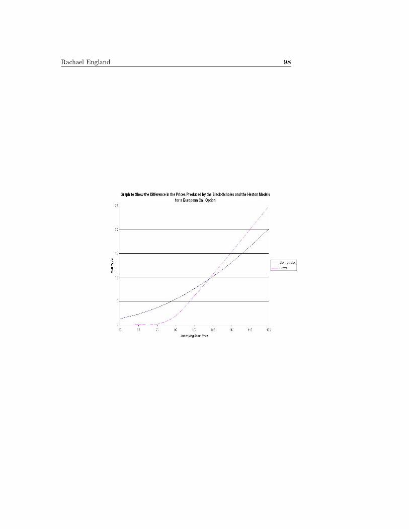
Rachael England 98
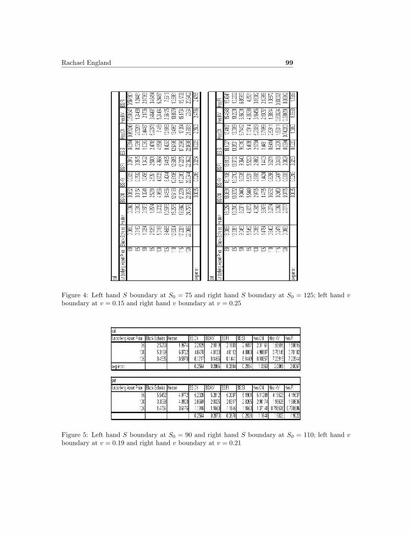
Rachael England 99
Figure 4: Left hand S boundary at S0 = 75 and right hand S boundary at S0 = 125; left hand vboundary at v = 0.15 and right hand v boundary at v = 0.25
Figure 5: Left hand S boundary at S0 = 90 and right hand S boundary at S0 = 110; left hand vboundary at v = 0.19 and right hand v boundary at v = 0.21

Rachael England 100
Figure 6: δ = 0.25, δv = 0.0025, δτ = 0.01

Rachael England 101
Figure 7: δ = 0.5, δv = 0.005, δτ = 0.001

Rachael England 102

Rachael England 103


![Variational Numerical Methods for Solving Nonlinear ...ultra.sdk.free.fr/docs/DxO/Variational Numerical Methods for Solving Nonlinear...given in [17]. In the discussion of the numerical](https://img.dokumen.tips/doc/110x75/5eda117fb3745412b570b4c9/variational-numerical-methods-for-solving-nonlinear-ultrasdkfreefrdocsdxovariational.jpg)