RAD-AI26 414 THE USE OF MATRIX DISPLACEMENT METHOD FOR VIBRATIONAL i/lI ANALYSIS OF STRUCTURES(U) CARNEGIE-MELLON UNIVI PITTSBURGH PR ROBOTICS INST W 0 HUGHES MAY 81

UNCLASSIFIED CMU-RI-TR-B2-6 F/G 28/1 Li

1.0 &_ _. L

Al. Si3 2 f

'lU1.25 1.4 111.6

MICROCOPY RESOLUTION TEST CHART 4"

NATIONAL BUREAU OF STANDARDS- I 963-A

S.

L: .11 ~ . -

THE USE OF MATRIX DISPLACEMENT METHOD FORVIBRATIONAL ANALYSIS OF STRUCTURES

William 0. Hughes

Department of Mechanical Engineeringand

The Robotics InstituteCarnegie-Mellon University- Pittsburgh, Pennsylvania 15213

Met

C, y'- .... THE9

ROBOTICSCMU-RI-TR-82-6 INSTITUTE

A WeFOd t ""

b". .. . -

-SECURITY CLASSIFICAl?"IO -wS P*AC 'Wh 9 m Do- Ent$ ,J)

REPORT DOCUMENTATION PAGE E READ IYSTRUCTIO.NFS

I. REPORT NUMBER D. GOVI ACCESSION No. 3. RECIPi ENT CATALOG NUMBER

CMU-RI-TR-82-6 , I Ni

4. TITLE (and Subtitle) S. TYPE OF REPORT & PERIOD COVERED

THE USE OF MATRIX DISPLACEMENT METHOD FOR Interim

VIBRATIONAL ANALYSIS OF STRUCTURES6. PERFORMING ORG. REPORT NUMBER

1. AUTHOR(W) S. CONTRACT OR GRANT NUMBER(e)

William 0. Hughes

3. PERFORMING ORGANIZATION NAME AND ADDRESS 10. PROGRAM ELEM4ENT. PROJECT. TASK .

Carnegie-Mellon University .AREA A WORK UNIT NUMBERS

The Robotics InstitutePittsburgh, PA. 15213

11, CONTROLLING OFFICE NAME AND ADDRESS 12. REPORT DATE -

May 1981Office of Naval Research 3. NUMBER OF PAGES

Arlington, VA 22217 31

- 14. MONITORING AGENCY NAME & ADRESS(I! diffetat from Controlliln Office) 15. SECURITY CLASS. (of thie report)

UNCLASSIFIED

s. DECLASSIFICATION/DOWNGRAOINGSCHEDULE

IS. 0ISTRIBUTION STATEMENT (o'ths Report)

17. DISTRIBUTION STATEMENT (of the abeedc entered In Block 20. It different from Report) •

Approved for public release; distribution unlimited

IS. SUPPLEMENTARY NOTES

19. KEY WORDS (Continue an reverle *toe if neceeary an d identify by block nnber)

20. ABSTRACT (Continue an revere aide It neceeowey and identify by block naorber)

D o 1473 EDITION Of I NOV 4S IS OBSOLETEDD , j. ,]UNCLASSIFIEDS/N 0102-014-66011 C

SE[CURITY CLAS$IFItC.ATION OF THIS PAGE (ieaen Dote gIeorM) -

777777-7-

The Use of Matrix Displacement Method for

* Vibrational Analysis of Structures

byWilliam 0. Hughes'

Department ot Mechanical Engineering andRobotics Institute

Carnegie-Mellon University VPittsburgh, PA 15213

May, 1981

ABSTRACT A study of the matrix displacement method for modeling' the vibrations ofstructures is presented in this report. The model can analyze both the free andforced vibrations of a structure. Static loading on a structure is treated as aspecial case of the forced vibration analysis.

The work was suppotted in part by Carnegie-Mellon University Internal funding, through a FordFoundation Research Grant, and by the Robotics Institute.

1Under the Supervision of Prof. W.L. Whittaker and Prof. AAJ Holzer

Table of Contents

1 Introduction 12 The Finite Element Method - Fundamental Concepts and Applications 13 Explanation of the Model 2

3.1 Equations of Motion 23.2 The Matrix Displacement Method 43.3 Specific Aspects of Model 5

4 The Model: Examples and Accuracy 74.1 Example 1: Free Vibration of a Fixed-Free Uniform Beam 94.2 Example 2: Free Vibration of a Fixed-Fixed Uniform Beam 104.3 Example 3: Forced Vibration of a Fixed-Free Uniform Beam 104.4 Example 4: Static Deflection of a Fixed-Free Uniform Beam 134.5 Example 5: Static Deflection of a Fixed-Free Non-Uniform Beam 15

5 The Extension of the Model to Model A Turbine Blade 186 Conclusion 21

I. Appendix I Influence Coefficient Method 24

II. Appendix II Variational Method 26

III. Appendix III Computer Code of Model 31

uAraou*i~ For_

i*rxs GRA&I

I-_ 1 C T ADTIC ] wU8=0

AV.ILt if it CA- e

~~~~~~~I .. ..- ,, [ :. o

List of Figures

Figure 1: The beam element and its forces, after Przemieniecki [7] 6Figure 2* Stiffness Matrix of Beam Element of Figure 1 [After Przmieniecki]. [1'he sheer 8

deformation parameters 0y and 0 can be considered to be zero.]Figure 3: Consistent Mass Matrix for a Beam Element (After Przemieniecki [7D. 9Figure 4: Example 1: Fixed-Free Uniform Beam. 9Figure 5: First five bending mode shapes of Example 1. •12Figure 6: First four axial mode shapes of Example 1. 14Figure 7: Example 2: Fixed-Fixed Uniform Beam. 15Figure 8: Example 3: Fixed-Free Uniform Beam With Dynamic Load. 15Figure 9: Magnitude versus Forcing Frequency for Example 3. 16Figure 10: Example 4: Fixed-Free Uniform Beam With Static Load. 17Figure 11: Static Deflection of a Uniform Beam, Example 4, 17Figure 12: Example 5: Static Deflection of a Fixed-Free Non-Uniform Beam. 18Figure 13: Static Deflection of a Non-Uniform Beam, Example 5. 19Figure 14: Element Stiffness Influence Coefficients (After White, et al [10D. 24

* Figure 15: Stiffness matrix of prismatic elements of Figure 14. 25Figure 16: Axial element, cross-sectional area A, modulus E. 29

iZ

List of Tables

Table 1: Uniform Beam Properties- 8Table 2: Natural frequencies (radians/sec) and Percentage Error (%) as a function of number of 11

elements for Example 1.Table 3: Calculated and Exact Natural Frequencies in Axial Mode. Calculated value used five 13

element model, for Example 2.Table 4: Calculated and Exact Values of Deflections for Example 4. 18

A 1W7

1 Introduction

-A study of the matrix displacement method for modeling the vibrations of structures is presented in this

report. The model can analyze both the free and forced vibrations of a structure. Static loading on a structure

* is treated as a special case of the forced vibration analysis.

A brief review of the Finite Element Method and its present use is first given. This is followed by a

discussion of the methodology of the matrix displacement approach and a description of the specific model

* used. Examples of the use of the model to analyze the frequencies and mode shapes of the free and forced

* response of a beam structure and the static deflections of a beam structure are shown and compared with the

closed form solutions. Finally, ways of extending the model to a more complicated structure, a turbine blade,

are discussed. Conclusions are then drawn.

2 The Finite Element Method -- Fundamental Concepts and Applications

There are many methods available today which perform the analysis of structures. For e"ample, in one

method the structure is described by differential equations. The differential equations are then solved by

analytical or numerical methods. Another method of analysis is the finite element method (FEM).

In this method, the structure is idealized into an assembly of discrete structural elements, each having an

assumed form of displacement or stress distribution. The complete solution is then obtained by assembling

these individual, approximate, displacement or stress distributions in a way satisfying the force equilibrium

equations, the constitutive relationships of the material, the displacement compatibility between and within

the elements and the boundary conditions of the structure.

Methods based on discrete element idealization have been used extensively in structural analysis.The early

I pioneering works of Turner, et al., in 1956 [1], and Argyris in 1960 [21 led to the application of this method to

* static and dynamic analysis of aircraft structures. Other fields of structural engineering, such as nuclear

reactor design and ship construction have since employed this method.

4 Nor is the idea of discrete elements limited in use to structural analysis only. Thc fundamental concept of

the finite element method is that any continuous quantity, such as displacements, temperature, or pressure,

can be approximated by a finite number of elements. Thus, this approach can be used to solve problems in

heat flow, fluid dynamics, electro-magnetics, fracture mechanics and seepage flow to name just a few other

.4 areas of usage.

2

The representation of a continuous structure by structural elements of finite size results in large systems of

algebraic equations. A convenient way of handling these sets of equations is by the use of matrix algebra,

which also has the advantage of being ideally suited for computations on high-speed digital computers. For

this reason, expressions such as "matrix methods of structural analysis" are sometimes used to describe the

method. More common though is the term "finite element method", which emphasizes the discretisation of

the structure.

The finite element method actually encompasses three classes of matrix methods of structural analysis. The

first is- the displacement (or stiffness method), where the displacements of the nodes are considered the

unknowns. The correct set of displacemehts results from satisfying the equations of force equilibrium. The

I second method is the force (or flexibility) method. Here the nodal forces are the unknowns and are found bysatisfying the conditions of compatible of deformations of the members. The third class of matrix method is

the mixed method, which is a combined force-displacement method.

One last comment on the finite element method in general is necessary. An error is introduced into the

solution of the original problem as soon as the continuous structure is replaced by discrete elements. This

error remains, even when the discrete element analysis is performed exactly. In general this error is reduced

by increasing the number of discrete elements, thereby decreasing the element size and thus giving a better

idealization of the continuous structure. Zienkiewicz, Brotton and Morton [3] suggest that the user may

determine the limits of his error by: "(a) comparison of finite element calculations with exact solutions for

cases similar to his specific problem; (b) a 'convergence study' in which two or more solutions are obtained

using progessively finer subdivisions and the results plotted to establish their trend or (c) using experience of

previous calculations as a guide to the treatment of the specific problem." Further information on matrix

structural analysis and the finite element method may be found in many sources. [4-11]

3 Explanation of the Model

The following discussion is divided into three sections. Firstly the equations of motion will be stated.

Secondly, the matrix displacement method for solving such equations will be described. Finally some specific

aspects of the particular model being used will be discussed.

3.1 Equations of Motion

The motion of a vibrating system, consisting of mass and stiffness, of n degrees of freedom can be

represented by n differential equations of motion. These equations of motion may be obtained by Newton's

second law of motion, by Lagrange's equation or by the Influence Coefficients method. Since the equations

*~- T. .

3

of motion, in general, are not independent of each other, a simultaneous solution of these equations is

required to calculate the frequencies of the system.

The matrix equation for the free vibration case is:

[K - 2M1] X [0] (1)

where

[K] represents the stiffness matrix of the structure,[M] represents the inertial (mass) matrix of the structure,

represents the set of eigenvalues of the equationscorresponding to the set of natural frequencies,

[XI represents the set of eigenfunctions of the equationscorresponding to the set of displacements

For the free vibration case the set of forces is just zero.

The matrix [K- 2M] is called the impedance matrix.

The matrix equation for the forced vibration case is:

[K- W MJ [XI [PJ (2)

where [P] represents the set of forces on the structure, and,of is the driving or forcing frequency.

The other terms are as previously defined.

Inspection of equations (1) and (2) reveals that neither contain damping terms. This is because structures

of immediate concern have very low damping (-1 x 10-4 critical damping).

An excellent treatment on the dynamics of structures is Clough and Pcnzien [14].

4

3.2 The Matrix Displacement Method

An outline of the application of the matrix displacement method in finite element analysis for the solution

of dynamic problems follows. A similar outline is given by Zienkiewicz, et a]. [31 for static analysis.

1. Input

a. Idealization of the problem

The continuous structure is divided into a number of elements. These elements areconnected at common nodal points or nodes. It is at these nodes that the value of thecontinuous quantity (displacement) is to be determined.

b. Preparation of the data for the structure

The geometry of the structure is defined by assigning coordinates to the nodal points. Thephysical properties of the elements (dimensions, material parameters) are inputted.

c. Preparation of the load data

The loads to be applied to each element or node are defined.

d. Preparation of the boundary conditions or constraints

The prescribed constraints on the degrees of freedom and boundary conditions are stated.

2. Processing

a. Element Formulation

The stiffness and inertial matrices for each element are determined by the approximaterelationships and the corresponding loads are calculated.

b. Assembly of the structure

The summation of the elemental matrices to form structural stiffness, inertial and load* matrices is performed.

c. Reduction of equations

The boundary conditions and constraints in terms of certain specified displacements areintroduced, thereby reducing the number of equations to be solved.

d. Solution. of simultaneous equations

The solution of the cigen problem of equation (1) or (2) results in the natural frequencies ofthe structure (eigenvalues) and the modal shapes or displacements of the nodes

0 (cigenfunctions).

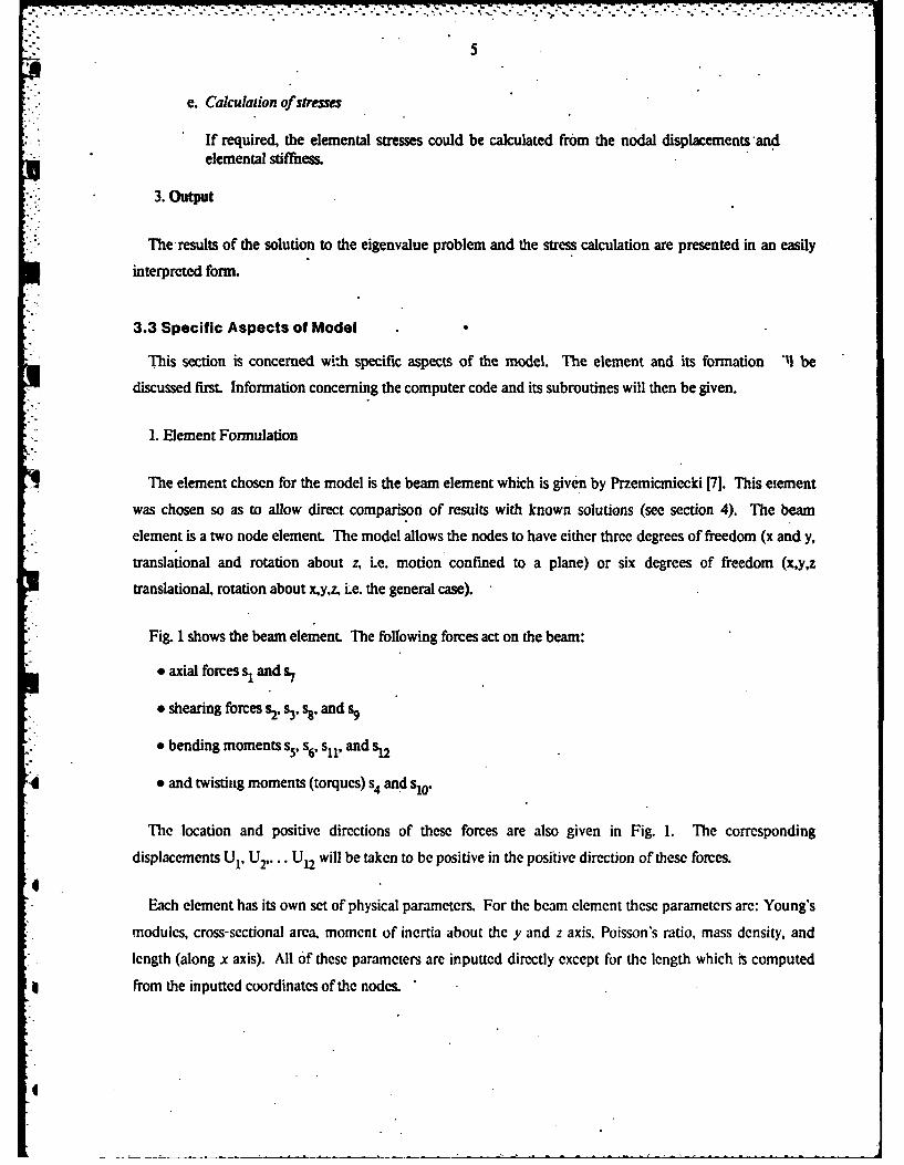
e. Calculation ofsIesses

If required, the elemental stresses could be calculated from the nodal displacements andelemental stiffness.

3. Output

-Theresults of the solution to the eigenvalue problem and the stress calculation are presented in an easily

interpreted form.

,. 3.3 Specific Aspects of Model .

This section is concerned with specific aspects of the model. The element and its formation "'l be

discussed first. Information concerning the computer code and its subroutines will then be given.

1. Element Formulation

The element chosen for the model is the beam element which is given by Przemicmiecki [71. This element

was chosen so as to allow direct comparison of results with known solutions (see section 4). The beam

element is a two node element. The model allows the nodes to have either three degrees of freedom (x and y,

translational and rotation about z, i.e. motion confined to a plane) or six degrees of freedom (x,y,z

translational, rotation about xy,z, i.e. the general case).

Fig. 1 shows the beam element. The following forces act on the beam:

* axial forces sI and &7

* shearing forces s2, s3, s8, and S9

* bending moments s5, s6, s1l, and s12

* and twisting moments (torques) s4 and sl0.

The location and positive directions of these forces are also given in Fig. 1. The corresponding

displacements U1, U2 .... U12 will be taken to be positive in the positive direction of these forces.

Each element has its own set of physical parameters. For the beam element these parameters are: Young's

modules, cross-sectional area, moment of inertia about the y and z axis, Poisson's ratio, mass density, and

length (along x axis). All of these parameters are inputted directly except for the length which is computed

from the inputted coordinates of the nodes.

I

~6

So

q S,0/ S9

/ 12

2 !/" Neutral axis

s2S4 S

0 Sz

Figure 1: The beam element and its forces, after Przemieniecki 1.

The model performs calculations for either the free or forced vibration case. To perform such calculations

requires the calculation of the structural stiffness and inertial matrices, along with information of the loading

and boundary conditions of the structure. The effect of constraining a degree of freedom is to strike out the

corresponding rows and columns of the stiffness, interial and load matrices.

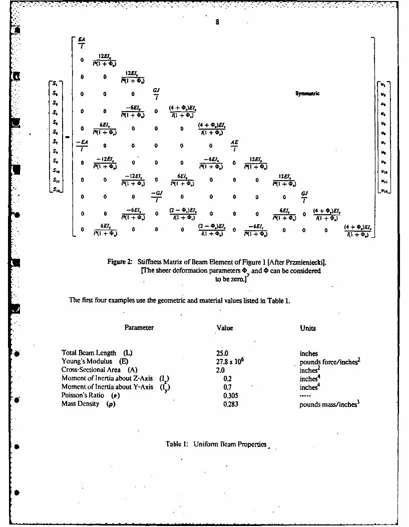
The sziffness matrix for a beam element is shown in Fig. 2. The shear deformation parameters 4) and 0

can be taken as zero. This matrix may be obtained in various ways. two of which are the influence coefficients

method and the variational method, which are outlined in Appendices I and II.

The inertial matrix for the beam element is shown in Fig.3. This matrix is obtained by the same methods as

* the stiffr--ss matrix, as described in Appendices I and II.

Liepe-s [131 gives a third way of calculating the stiffness and inertial matrices.

The s-uctural matrix for both stiffness and inertia is obtained by superposition of the individual elemental

matrices. Actual superposition occurs only when degrees of freedom are common to more than one element.

2. Corputer Coding

The c :,rnputer code itself contains ten subroutines, called by the main program, entitled VIBRAT. A brief

cxplanatf-on of the subroutines will now be given.

0

). .

7

INPUT - This subroutine asks the user ior the necessary information which is needed to assemble thestructure. Information such as: free or forced case, number of elements, coordinates ofnodes, physical parameters, structural loading, and constrained degrees of freedom areinputted in this section.

- CONECT - This subroutine establishes the geometry of the model. It determines the distances betweenadjacent nodes of the structure.

* KMAT - This subroutine calculates the elemental stiffness matrix for each element and then assembles the

structural stiffness matrix from them.

MMAT -This is similar to KMAT only here the mass or inertial matrices are calculated.

EIGEN - This subroutine is called for the free vibration case. The purpose of it is to calculate the eigenvalues(natural frequencies) and eigenvectors (mode shapes) of equation (1). This subroutine callstwo other subroutines: EIGZF, an IMSL routine which actually does the solving, andCLAMPR, which determines which degrees of freedom are constrained.

SOLVE - This subroutine is called for the forced vibration case. This routine solves equation (2) for thedisplacement. This subroutine also calls two other subroutines: LEQT1F, an IMSL routinewhich does the solving, and CLAMPR, which determines the proper degrees of freedom tobe constrained.

" REMARK - is a subroutine whose purpose is to explain the use of the main program VIBRAT and itssubroutines. Information on the nomenclature and file structure used can be found inREMARK. The user of the model is recommended to refer to REMARK if he has anyquestions on the computer code used in this model.

The code for all of these routines may be found in Appendix Ill.

4 The Model: Examples and Accuracy

This section presents various examples of use of the model. The examples chosen represent five types of

possible problems. They are:

1. free vibration of a fixed-free uniform beam

2. free vibration of a fixed-fixed uniform beam

3. forced vibration of a fixed-free uniform beam

4. static deflection of a fixed-frec uniform beam

5. static deflection of a fixed-free non-uniform beam.

The accuracy of each example is discussed.

8

FA"" ' T

o 1211.'0'1N +'0 0 12E,o o -E E1.)

". SI -- J -

St 0 0 0 - symmdric

:- - I, + Us

o Mo + 0 a) 1(+0.) K6( E

s 0 0)- 6E). 0 0 0 (4 + O.),1. (+ I"s

so +, +) 1(1+0,) ,S". , -E"A 0 0 0 0 0 LA£ n,

F e isE t oI I 1

so 0 -12t 0 0 0 -6E b 0 12z e ,

The fis fou exmpE. use Mhe gemti aNd mae+a vauslseOnbl 1., t

ot a + Le nh + (L) )0 0 + 2. i

Momcn 0 0 0 60_ 0.2 0 i2ces

omtf+ lnctiaabot YAi I + 0) .7 inchePois son0s Rai , 03 05 0 )ErS 0a0 0 Density0( 0 .20 0 n ms/ce

LT bl + Un) f(o + (a,) Po +

I Figure 2: Stiffness Matrix of Beam Element of Figure 1 [After Przmieniecki].[The sheer deformation parameters 0 y and 0) can be considered

to be zero.]

~The first four examples use the geometric and material values listed in Table 1.

Parameter Value Units

i"" Total Beam Length (L) 25.0 inchesSYoung's Modulus (E) 27.8 x 10 pounds force/inches2

Cross-Sectional Area (A) 2.0 inches 2

•Moment of Inertia about Z-Axis (Iz) 0.2 inches 4

.Moment of Inertia about Y-Axis (I Y) 0.7 inche 4

Poisson's Ratio (P) 0.305 -----e"Mass Density (p) 0.283 pounds mass/inches 3

• Table 1: Uniform Beam Properties.

9

I

20 !!~,13+ j.i

0 0 13 +61.S30 0SAP

40 0 Symmetric

PAI

J f 70 o p 2,,

7!1 0 0 0 0 06 3

0 6 131 1. 0 13 1

_L0 0 0 0 ~ IA70~3 SAA40L'A

100 000 0 0 0 0

20 00 5A 3A

131 1, + 21,

0 0 ... !..~0 0 0 0420 1041I 140 30A 210 1041 105 I SA

0 131 + . 0 0 00 1_____ 0 0 P 21 + 21.20 -- A+- 0 0 0 30A 210 104. 0 1

42 IoA __,________ ___o_____ [ s

2 4 7 . 9 0 10 32

Figure 3: Consistent Mass Matrix for a Bcam Element

(After Przemieniecki liD.

4.1 Example 1: Free Vibration of a Fixed-Free Uniform Beam

Figure 4: Example 1: Fixed-Fre Uniform Beam.

Table 2 summarizes thc results for this problem. using onc, two, and five elcments. It is clear that

10

increasing the number of elements increases the accuracy of die results, and this supports the statements of

Zienkiewicz given earlier.

The natural frequencies calculated by the model are compared with the closed form solution obtained

from the -partial differential equation of the continuous system. For the fixed-free case the closed form

solutions are:

Axial = -- -- where n = ,3,5,... (3)2L p

Bending(i) W= aLO/----'- where 1 + cos aL cosh aL =0pAL4

i=YorZ (4)

Torsional W = -- C 7 where n =1, 3, 5 ... G - (5)

2L p 2(1+v)

Thus from Table 2, one can see that by using just five elements, the model gives ten transverse modes, two

axial modes, and two rotational modes, the frequencies of which are all within 5% of the exact solutions.

Again, clearly greater accuracy of results and more (higher) modes may be accomplished by increasing the

number of elements.

Diagrams of the mode shapes for the first five bending modes (in Y) and the first four axial modes (along

X) are given in Figs. 5 and 6. The model shapes agree with the closed form predictions in every case.

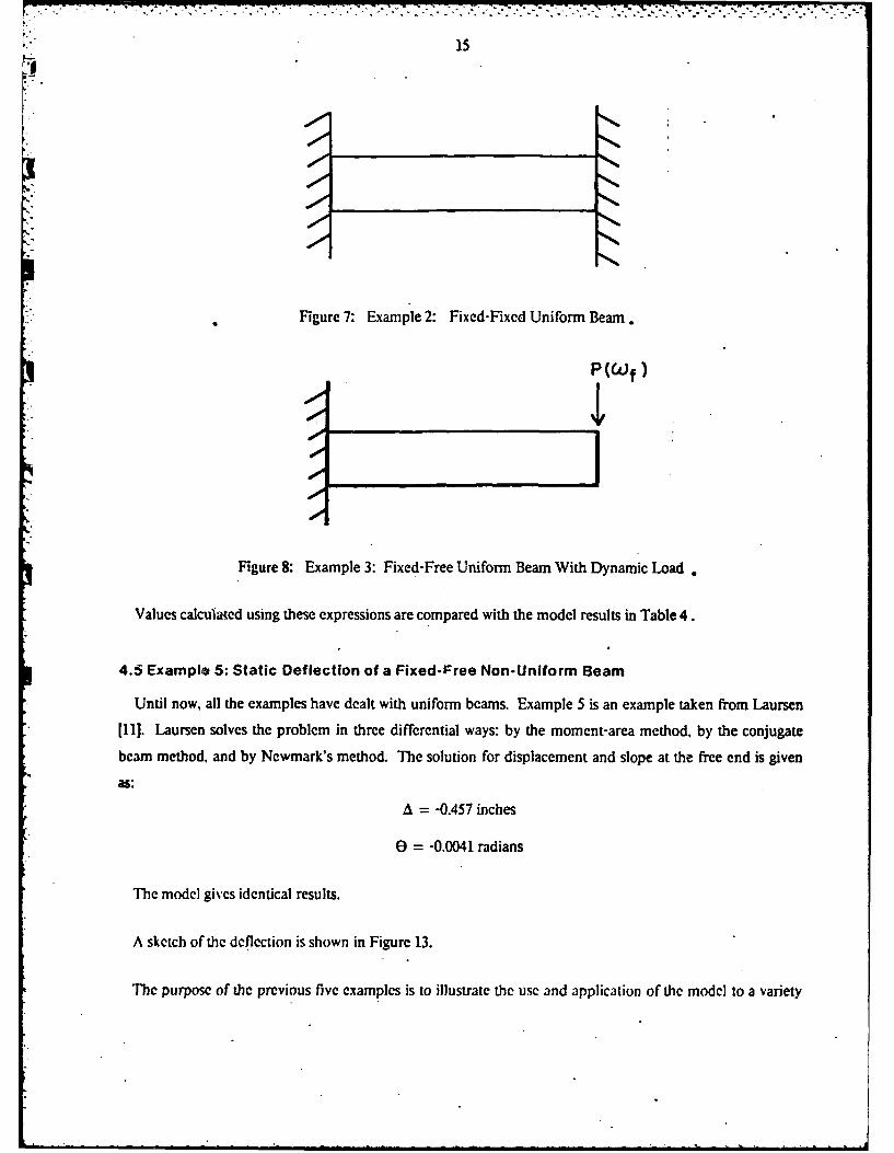
4.2 Example 2: Free Vibration of a Fixed-Fixed Uniform Beam

In this example the beam is held fixed on both ends. See Figure 7 . Table 3 shows the calculated and exact

values for the axial mode natural frequencies. The accuracy is similar to that of example 1.

6

4.3 Example 3: Forced Vibration of a Fixed-Free Uniform Beam

In this example (Figure 8), the beam is subjected to a harmonically varying load P(t) of amplitude P and

circular frequency, wf. Figure 9 is a plot of the magnitude in the transverse direction of the free end node. As

expected, as wf approaches a natural frequency (those found in example 1), a resonance condition occurs

rejlting in *very large magnitudes of deflection. The expression for the amplitude of response A is given by

6,

C4 0; Ot', oc

4a ,-4,-

U) 4) in m'i -4 r n - %OLL. L) %D t-' f r-O~f ) I ifl-4 %0 -4

a) )L (4- 00 -4r- r- 0 Gor, -qT

C'' O0 C1t'8Lf4%

N..- V4) f 0 mN00 m-4 -4 00V lT00r r4-n.nMto1%0 D *D n CD 10 .D % . 0-% C 4

r-4 t4) -inc l car-400r4 M -4o _- on

go 0

ccE

t)C

on e4n

t4a in 00Me. )0m 'g Dmr- 0- c '

Lz ~a C I "1r- %0 t-)-r-4 a al o

=ca

aimA %0' in

'-44

0 w)

C14~ CL r-ini

E- x

4 ) Lz LL)

127 -777

2

-4/-

0 1

Figure 5: First five bending mode shapes of Example 1

13

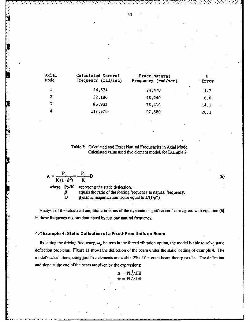
Axial Calculated Natural Exact NaturalMode Frequency (rad/sec) Frequency (rad/sec) Error

1 24,874 24,470 1.7

2 52,186 48,940 6.6

3 83,933 .73,410 14.3

4 117;570 97,880 20.1

Table 3: Calculated and Exact Natural Frequencies in Axial Mode.Calculated value used five element model, for Example 2.

p pA P =--:-P D (6)' K (1-pf2 ) K

where Po/K represents the static deflection,Pl equals the ratio of the forcing frequency to natural frequency,D dynamic magnification factor equal to 1/(1-l2)

Analysis of the calculated amplitude in terms of the dynamic magnification factor agrees with equation (6)

in those frequency regions dominated by just one natural frequency.

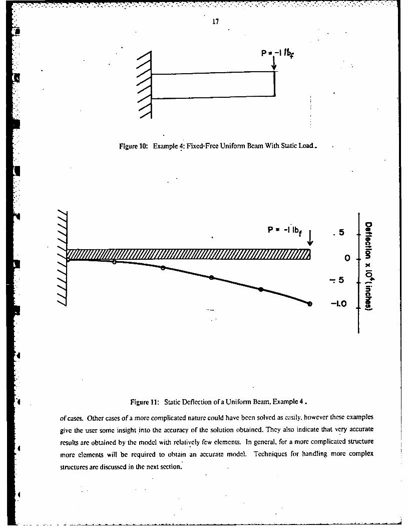
4.4 Example 4: Static Deflection of a Fixed-Free Uniform Beam

By letting the driving frequency, w, be zero in the forced vibration option, the model is able to solve static

deflection problems. Figure 11 shows the deflection of the beam under the static loading of example 4. The

model's calculations, using just five elements are within 2% of the exact beam theory results. The deflection

and slope at the end of the beam are given by the expressions:

= PL3/3EI0 = PL2/2EI

-:7-, -C. 7777

41

0-0

I--

K 1.5

Figure 7: Example 2: Fixed-Fixed Uniform Beam.

P(Wf)

7"4,,

Figure 8: Example 3: Fixed-Free Uniform Beam With Dynamic Load

Values calculated using these cxpressions are compared with the model results in Table 4.

4.5 Example 5: Static Deflection of a F ixed-Free Non-Uniform Beam

Until now, all the examples have dealt with uniform beams. Example 5 is an example taken from Laursen

* 1i1]. Laursen solves the problem in three differential ways: by the moment-area method, by the conjugatebeamn method, and by Newmark's method. The solution for displacement and slope at the free end is given

as:

A =-0.457 inches

0 =-0.0041 radians

The model gives identical results.

A sketch of the deflection is shown in Figure 13.

The purpose of thc previous five examples is to illustrate the use and application of the model to a variety

0800,000

w

0

' I

0 500 1,000 1,00p(1*4.72,000 2,500 3100U3Jf CJs -2165.93 (rod/i)

Figure 9: Magnitude vcrsus Forcing Frequency for Example 3.

17

S PU

Figure 10: Example 4: Fixcd-Free Uniform Bcan With Static Load.

- 0

0

. 5.

• -1.0 1

4.[ Figure ll: Static Deflection of a Unifonn Beam, Example 4.

of cases. Other cases of a more complicated nature could have been solved as asily. however these examples

give the user some insight into the accuracy of the solution obtained. They also indicate that very accurate

results arc obtained by the model with relatively few elements. In general, for a more complicated structure

more elements will be required to obtain an accurate model. Techniques for handling more complex

structures arc discussed in the next section.

4t

18

A (inches) 8 (radians)

Exact -9.37 x 10 -5.62 x 10- 5

Calculated -9.50 x 10 -5.69 x 10-

% 1.4 1.2

Table 4: Calculated and Exact Values of Deflections for Example 4,

5 kipsL BI

I - SOO in." I-50in.6ft 9 ft

Figure 12: Example 5: Static Deflection of a Fixed-FreeNon-Uniform Beam.[After Laursen].

5 The Extension of the Model to Model A Turbine Blade0

An example of a morc complicated structure which might be of vibrational interest to an engineer is a

turbine blade. The equations of motion for a beam in bending vibration is a fourth-order differential

equation. whose solution is easily found. The solution for a non-uniform and asymmetrical beam is much

more complicated. A tapered, prc-twistcd turbine blade with airfoil cross-section might be modeled as such a

beam.

The differential equations for combined flapwise bending, chordwise bending and torsion of a twisted

non-uniform blade are derived by Houbolt and Brooks f161. The solutions of these equations for the

continuous system have not been found. ilius the analysis of such structures are limited to special cases

0J

19

.5-~

000

0

.25 j(8

Figurel13 Static Deflectionx of a Non-Uniform Beam, Example 5.

20

which solutions are obtainable, or to approximate solutions. Various techniques of an analytical and iterative

* nature such as the Mykiestad method, Holzer method. Stodala method, Rayleigh-Ritz method, transmission

matrix method, and the Runge-Kutta method have been studied [14]. A few typical examples are given in the

* references [15,17-201.

The application of the model presented in this report to the turbine blade would be a very useful tool to the

engineer and his study of the blade's free and forced vibrations.

The model allows each element t6 have its own set of geometric and physical parameters. Thus neither the

non-uniformity or tapering of the blade would lead to any modeling problems. H~wever the airfoil shape of

the blade would not have the same torsional stiffness as a beam. Thus the first adaptation to the modelneeded would be to correctly compute the torsional stiffness for an airfoil shape and input this into the model

rather than using that which the model computes.

There is another problem which arises from the twisting and geometry of the turbine blade. The natural

frequencies of such a blade are coupled frequencies with the mode shapes consisting in general of tr ansverse

motion coupled with torsion. The coupling is dependent upon the degree of pre-twist and the ratio of depth

taper to width taper. For a given. blade, coupling becomes stronger with increasing pre-twist and with

increasing width to depth taper ratio.

The simulation of this coupling in the mode[ could be accomplished by either introducing it through the

element itself or through the geometry of the structure. The first way implies changing the element from a

beam element to a new element. This new element could be derived from a variational method (see

Appendix 11) applied- to the differential equations for the blade equations derived by Houbolt and Brooks

[16]. The ideal of coupling through the geometry of the structure implies the use of additional beam

elements. Part of these elements would be used to form the center of stiffness for the blade which would now

* be a curve rather than the straight line used thus far. Other elements could extend at right angles from this

curve. These elements would act primarily as lumped masses and form the curve representing the center of

mass of the blade.

4 Modeling a turbine blade with this model would require some additional work to implement the ideas

presented in this section. However the matrix displacement method used is a very powerful one and the use

of the model and extensions of it are applicable to a wide range of problems in vibrational analysis of

structures. Building a libraiy of elements would greatly extend the usefulness of the existing .model, and

4 additionally, the introduction of element rotation would lead to further improvement.

4

* 21

6 Conclusion

This report primarily concerns itself with three topics:

1. the explanation of the matrix displacetnent method for use in vibrational analysis of structures,

2. specific examples showing the variety and accuracy of the method, and

3. possible extensions of the model to allow for application to an even wider variety of problems.

The model presented here currently allows for only one type of element, the beam element. It has been

shown that by using just a few beam elements very accurate results of frequencies and modal shape are

* obtained for beam-like structures. Creating a library of element types would allow the user -even greater

flexibility. The accuracy of the model using these new elements should be comparable to that presented here.

22

Acknowledgements

The author is grateful to Prof. Alex J. Holzer, who acted as advisor throughout this study. Special thanks

also goes to Prof. William L. Whittaker of the Department of Civil Engineering at Carnegie-Mellon

University, for the help, guidance and encouragement given.

References

1.) M. J. Turner, R. W. Clough, H. C. Martin, and L. J. Topp, "Stiffness and Deflection Analysis of ComplexStructures", Journal of the Aeronautical Sciences, Volume 23, Number 9, September 1956, pp. 805-823.

2.) 1. H. Argyris, "Energy Theorems and Structural Analysis", Butterworth Scientific Publications, London,1960.

3.) 0. C. Zienkiewicz, D. M. Brotton, L. Morgan, "A finite element primer for structural engineering", TheStructural Engineer, Volume 54, Number 10, October 1976, pp. 387 - 397.

4.) J. S. Przemieniecki. "Matrix Structural Analysis of Substructures:", American Institute of Aeronautics andAstronautics Journal, Volume 1, 1963, pp. 138-147.

5.) J. B. Spooner, "Finite element analysis: development toward engineering practicality", The CharteredMechanical Engineer, Volume 23, Number 5, May 1976, pp. 96-99,101.

6.) T. H. H. Plan, "Variational and Finite Element Methods in Structural Analysis", RCA, Review, Volume39, Number 4, December 1978, pp. 648-664.

7.) J. S. Przemieniecki, "Theory of Matrix Structural Analysis", McGraw-Hill Book Company, 1968.

8.) R. H. Gallagher, "Finite Element Analysis Fundamentals", Prentice-Hall, Inc. 1975.

9.) L. J. Segerlind, "Applied Finite Element Analysis", John Wiley & Sons, Inc., 1976.

10.) R. N. White, P. Gergely, R. G. Sexsmith, "Structural Engineering, Combined Edition", John Wiley &Sons, Inc., 1976.

0.11.) H.I. Iaursen, "Structural Analysis", McGraw-Hill Book Company, 1969.

12.) J. S. Archer, "Consistent Mass Matrix for Distributed Mass Systems", Journal of the Structural Division,Proceedings of the American Society of Civil Engineers, Volume 89, Number ST4, August 1963, pp.

* 161-178.

13.) A. A. l.icpins, "Rod and Bcam Finite Flement Matrices and Their Accuracy", American Institute of

Aeronautics and Astronautics Journal, Volume 16, Number 5, May 1978, pp. 531-534.

14.) R. W. Clough, J. Penzicn, 'Dynamics of Structures", McGraw-Hill Book Company, 1975.

15.) W. Carncgic, J. Thomas. "The Coupled Bending-Bending Vibration of Pre-Twisted Tapered Blading",

0 '+. . . .-. .

23

Journal of Engineering for Industry, Transactions of ASME, Volume 94, Series B, February 1972, pp.255-266.

16.) J. C. Houbolt, G. W. Brooks, "Differential equations of motion for combined flapwise bending,chordwise bending, and torsion of twisted non-uniformed rotor blades", NASA Report 1346. 1958.

17.) V. R. Murthy," Dynamic Characteristics of Rotor Blades", Journal of Sound and Vibration, Volume 49,Number 4, 1976, pp. 483-500.

18.) W. Carnegie, B. Dawson, J. Thomas, "Vibration Characteristics of Cantilever Blading", Proceedings ofthe Institution of Mechanical Engineering, Volume 180, Part 31, 1965-1966, pp. 71-89.

19.) E. Dokumaci, J. Thomas, W. Carnegie, "Matrix Displacement Analysis of Coupled Bending-BendingVibrations of Pre-twisted Blading", Journal of Mechanical Engineering Science, Volume 9, Number 4,1967, pp. 247-254.

20.) J. Montoya, "Coupled Bending and Torsional Vibrations in a Twisted, Rotating Blade", The BrownBoveri Review, Volume 53, Number 3, 1966, pp. 216-230.

4,

4

a - " • : -" I " " I I I |

24

1. Appendix I Influence Coefficient Method

One method of obtaining the stiffness matrix is the influence coefficient method. This method is widely

used in structural analysis with* static loadings [10,11]. There are both stiffness and flexibility influence

coefficients: only the stiffncss influence cocfficients will be considered here.

The stiffness coefficients for an element are found by alternatively constraining all degrees of freedom but

one and displacing this one by a unit amount The resulting forces on the other degrees of freedom are the

stiffness coefficients. That is Ktj is the force or couple corresponding to degree of freedom t due to the unit

displacement of degree of freedom j. In Fig. 14 a prismatic element of length 1, area A, moment of inertia

about the Z axis I, and modulus of elasticity E with three degrees of freedom per node is shown.

2

(a)

A AA

C.0,f. A d.o.f. #4

12RI 12E16E1 13

- . . 6/ 6£1I-z I- iA ~

of 2 _ d.a.f. #5

E6E

d.o.f. #6(b)

Figure 14: Element SUffncss Influence Coefficients (After White, et al 1101).

BBy performing the stiffness influence method procedure on this clement, the stiffness matrix is obtained:

6,

25

EA -EAEA 0 0 -A 0 0

12EI 6E -12EI 6El

6E1 4E --6EI 2E1|D = -EA EA

_ A 0 0 E A 0 0

o 12El -6E 0 12E1 -6EI0 13 12 0 73 1 2

6E1 2E 0 -6El 4El0 i1 1 0 l-..- 1

Figure 15: Stiffness matrix of prismatic elements of Figure 14.

Comparison of Fig. 2 and 15 shows that the matrix of Figure 15 is contained within the matrix of Figure 2.

In Fig. 15, each node has three degrees of freedom, in Fig. 2 there are six degrees of freedom per node.

The incrtil (or mass) matrix may be calculated similarly. The mass influence coefficients would represent

the mass inertia force acting at a degree of freedom due to a unit acceleration of another degree of freedom.

.-

26A

i. Appendix II Variational Method

Another mcthod of computing elcmcntal stiffness matrices is the variational or energy method commonly

used in finite clement programs. The outline presented here largely follows that of Gallagher 18].

The principle of minimum potential energy furnishes a variational basis for the formulation of the element

stiffness matrix. The potential energy (7y) of a structure is given by the strain energy (U) plus the potential of

the external work V (V = -Wext). .The theorem of potential energy is: of all displacements, satisfying the

boundary conditions, those that satisfy the equilibrium conditions make the potential energy assume a

stationary (extreme) value. Thus

WP = U + V (7)

8WP = SU + 8V = 0 (8)

And for stable equilibrium, 7rp is a minimum.

S17p = 2 U + 5 2V > 0 (9)

The change in strain energy density due to the change in strain caused by a virtual displacement (Be) is given

by

8 (dJ) = Be (10)

Where a is the equilibrium stress state prior to the application of the virtual displacement. The stress--strain

law is

a = [Ele - [Eje int (11)

where JE] is called the material stiffness matrix, a matrix of elastic constants. For simplicity, let there, be no

initial strain. Substitution of(11) into (10) yields

4 dl = e[E] e (12)

Integration between zero and the strain e, corresponding to a, gives

1dU C- [Ee (13)

2

-|

27

and integration over the volume of the element results in

U .f e[E]e d(vol) (14)[ 2 fV0

The variation of U is

8U = f c[E] Se d(vol) (15)vol

The potential of the applied loads is

V=-xFAj T -. Uds (16)Sa

where FL represents point forces, and T are traction forces on the surface. The variation of V is

vf= xF 1 ,. i. ids-Y (17)Sa

Using the minimum potential energy theorem (equation 8) results in

f ,,E]8 d(vol) + FAf 81lds= ()vol sa

In the finite element matrix, the displacements, [A], are written as a polynomial matrix times a vector of

, parameters in the assumed displacement field.

[A] = [P] [a] (19)

[P] evaluated at the node gives a matrix [B], consisting of constants. Thus

[Anodes) = [B] [a] (20)

Inverting to find [a] in (20) and substitution into (19) leads to

[A] = [P] [11 [Anodes]

[ [N] Anodes (21)

where N is the shape function. The shape function N has the quality that it is equal to I when evaluated atthe geometric coordinates of the point at which A is defined and is equal to zero at all other degrees-of-

freedom A,, J *I.

28

The matrix [D] is called the dof-to-strain transformation. Then

[e =DI [Anodes] (22)

For example if,

iau7 .L then

ax

[D= [N" ] (23)

Substitution of these ideas into (18) leads to

f [DJt [EI[D]A noesdVol(SAnodes t)- I[N'FL(8Anodes)Vol

- f [Nl t[Tlds(SAnodest) =0 (24)S

dividing (24) by Anodest results in

[K] Anodes - Fext = 0 (25)

where

Vo[K] = l [D]t[E] [DIdvol

[NtT ~(26)

Fext [Nlt[T]dS + ,[Ni]tF i (27)

i Thus the stiffness matrix can be found by equation (26).

As an example take the axial element show in Figure 16, with dofAl and A2 only. The procedure to

calculate the stiffness of this element follows. LetI

I

o

29

Figure 16: Axial elcmcnt, cross-sectional area A, modulus E.

C' d :

§L [ z

b--

A 2

The result is also contained in the stiffness matrices shown in Figures 2 and 15.

The inertial (or mass) matrix can also be calculated by use of this method. The variational approach leads

to

[MI [N [p][NfdVol (28)

Id

30

where [p 3is the material mass density matrix. Since the shape functions used here are the same as those

used for the stiffness calculation the result i's called the consistent mass matrix. A consistent mass matrix is

more accurate than a lumped mass approach [121.

* 31

Ill. Appendix Ill Computer Code of Model

Available from Author.

I

I

I