The Urban-Brookings Tax Policy Center Microsimulation Model

The Urban-Brookings Tax Policy Center Microsimulation Model: Documentation and Methodology for Version 0304

Jeffrey Rohaly

Adam Carasso

Mohammed Adeel Saleem

January 10, 2005

Jeffrey Rohaly is a research associate at the Urban Institute and director of tax modeling for the Tax Policy Center. Adam Carasso is a research associate at the Urban Institute. Mohammed Adeel Saleem is a research assistant at the Urban Institute. This documentation covers version 0304 of the model, which was developed in March 2004. The authors thank Len Burman and Kim Rueben for helpful comments and suggestions and John O’Hare for providing background on statistical matching. Views expressed are those of the authors and do not necessarily reflect the views of the Urban Institute, the Brookings Institution, their boards, or their sponsors.

Documentation and Methodology: Tax Model Version 0304

2

A. Introduction.................................................................................................................... 3

Overview................................................................................................................................. 3

History..................................................................................................................................... 5

B. Source Data.................................................................................................................... 7

SOI Public Use File ................................................................................................................ 7

Secondary Data Source: The Current Population Survey....................................................... 9

Creating Tax Units in the CPS.............................................................................................. 10

Statistical Matching of SOI and CPS data ............................................................................ 13

Imputation of Other Variables .............................................................................................. 18

Aging and Extrapolation ....................................................................................................... 24

C. Tax Calculator............................................................................................................ 29

The Parameter File................................................................................................................ 29

Calculating Individual Income Tax Liability........................................................................ 31

Effective Marginal Tax Rates ............................................................................................... 33

Other Federal Taxes.............................................................................................................. 34

Model Output ........................................................................................................................ 38

Case Model ........................................................................................................................... 41

Appendix A: Retirement Savings Module.................................................................................... 48

Appendix B: Description of Income Measures............................................................................. 59

Appendix C: Estate Tax Methodology ......................................................................................... 61


3

A. Introduction

The Urban-Brookings microsimulation tax model is a powerful tool for federal tax policy

analysis.1 The model calculates tax liability for a representative sample of households, both

under the rules that currently exist (current law) and under alternative scenarios. Based on these

calculations, the model produces estimates of the revenue consequences of different tax policy

choices, as well as their effects on the distribution of tax liabilities and marginal effective tax

rates (which affect incentives to work, save, and shelter income from tax). The model is also a

useful input to research on the effects of taxation on economic behavior.

Overview

The Urban-Brookings Tax Policy Center model is a large-scale microsimulation model of

the U.S. federal tax system. The model is similar to those used by the Congressional Budget

Office (CBO), the Joint Committee on Taxation (JCT), and the Treasury’s Office of Tax

Analysis (OTA).

As its name suggests, a microsimulation model uses microdata—or data on individual

units—rather than aggregate information.2 In general, input data are comprised of detailed

information at the individual or household level that may be used to calculate tax liability. The

sample includes weights that represent how many units are represented by the individual record.3

1 This document details the methodology underlying version 0304 of the model, which was developed in March 2004. The Tax Policy Center will publish revised versions of this paper as it updates the model. 2 For a detailed explanation of microsimulation models, see http://trim.urban.org 3 The weights equal the inverse of the sampling probability. Thus, for example, if a record was sampled at a rate of 1 in 1,000 (so the probability equals 0.001), the sample weight would be 1,000. In other words, that record represents 1,000 individuals or households.


4

Estimates for the entire population may then be derived by multiplying the individual estimates

by the sample weights and summing them.

In the case of the tax model, the population is the universe of individuals who file income

tax returns as well as those individuals whose incomes are too low to require them to file a return

(“nonfilers”). The data are a stratified sample of individual income tax returns augmented by

information about nonfilers (see discussion below). The tax-calculator portion of the model then

applies applicable tax law to each of the individual records in the microdata file and calculates

values for variables such as adjusted gross income (AGI), nonrefundable credits, individual

income tax liability, and so on. The values of the variables calculated for each individual record

are then multiplied by the weight associated with that record to tabulate aggregate results such as

total income tax liability for the entire population.

The tax model is not only able to calculate tax liability under current tax law but is also

able to simulate alternative policy proposals. It is therefore straightforward to calculate the

change in aggregate tax liability from a tax policy proposal and also to determine which class of

individuals would benefit from or bear the burden of the tax change.4

4 We note two items here: (1) static versus dynamic estimates and (2) statutory versus economic incidence. First, the revenue estimates produced by the model are purely static in nature. A static revenue change ignores the impact of any change in behavior that a policy proposal could cause and also does not take into account any macroeconomic effects of the proposal. For example, an increase in the top statutory marginal tax rate could cause a shift in compensation away from taxable wages and salaries toward untaxed fringe benefits. A purely static analysis would not capture this effect and would likely overestimate the potential revenue gain. Revenue estimates produced by JCT typically include the effect of behavioral changes but not the macroeconomic feedback effects. Behavioral responses can also change the burden of a tax change. For example, the burden of a tax increase on individuals may be smaller than the static change in tax because taxpayers change their behavior to avoid the tax. Thus, static distributional tables tend to overestimate the economic burden of tax increases and underestimate the burden of tax cuts.

Second, burden estimates reflect the statutory incidence—that is, the direct effect on individuals who pay the tax. The economic incidence of the tax may be different. For example, wage subsidies such as the earned income tax credit (EITC) may partially benefit employers who may be able to pay EITC recipients a lower wage. In that case, the economic incidence of the tax would be shared between the direct recipients (low-wage workers) and the indirect beneficiaries (their employers).


5

The tax model also has the ability to produce estimates for years beyond the year of the

input data file (currently 1999). This is made possible by “aging” the individual records in the

microdata file. In the aging process, the information on each record—such as the amount of

wages and salaries and other forms of income—as well as the weights associated with each

record are adjusted based on forecasts from several sources including CBO and the Bureau of the

Census.

History

The TPC produced the first version of its microsimulation tax model in 2002.5 Some of

the early research that used estimates produced by the model included an analysis of the effects

of the Economic Growth and Tax Relief Reconciliation Act of 2001 (EGTRRA) on low-income

families and children as well as a detailed study on the looming problem of the alternative

minimum tax (AMT).6

A more comprehensive version of the tax model was put in place in the spring of 2003.

This updated version improved the original model and expanded its scope in several ways. First,

we updated the input data to incorporate the most recent microdata file available from the IRS.

Second, we updated our projections and forecasts using the latest economic data available from

CBO. Finally, we added the capability to carry out distributional analysis on the entire

population by adding nonfilers for the first time, through a statistical match with the Current

Population Survey (CPS).

5 John O’Hare and Frank Sammartino were instrumental in developing and programming this first version of the model. 6 See Burman, Maag, and Rohaly (2002) and Burman et al. (2002).


6

The most recent version of the model was developed in March 2004 and includes the

latest economic forecasts from CBO as well as several model enhancements. First, we added a

retirement savings module that, among other things, imputes contributions to tax-deferred

savings vehicles such as IRAs (both traditional and Roth) and 401(k) plans. Second, we added an

estate tax module to the model that allows us to calculate the expected value of net estate tax

liability for each record in the tax model database. We also began distributing the burden of the

corporate income tax to individuals. Through these improvements, the distribution tables

produced by the TPC now include the following federal taxes that in 2003 accounted for about

93 percent of all federal tax revenues: individual and corporate income; payroll; and estate (CBO

2004). Third, we developed two measures of income for our distribution tables that are broader

than adjusted gross income (AGI), the qualifier that we used in tables produced by the first two

versions of our model. One measure is similar to the income concepts used by Treasury, JCT,

and CBO; the other is a broad measure of economic income similar to the one used at Treasury

until 2001.

We are currently producing an education module for the model that will allow us to

estimate the revenue and distributional effects of the various education provisions in the tax

code. We will also continue to update the model using the latest economic and demographic

forecasts and projections, as well as the latest microdata released by the IRS.


7

B. Source Data

SOI Public Use File

The primary data source for the tax model is the 1999 Public Use File (PUF) produced by

the Statistics of Income Division (SOI) of the Internal Revenue Service (IRS).7 The PUF

contains 132,108 individual records, sampled from the 127.1 million individual income tax

returns filed for tax year 1999. The records in the PUF are a stratified probability sample; the

population of tax returns is divided into subpopulations (strata), from which the samples are then

independently selected. The weights associated with each sample are calculated by dividing the

total number of returns in a stratum by the number of sample returns for the stratum.

Each record in the PUF has 38 indicator codes and 199 quantitative fields. The indicator

codes are descriptive in nature and provide information such as filing status, the number of

dependent exemptions, and whether or not certain forms such as those for the alternative

minimum tax, the child and dependent care credit, and the general business credit are attached to

the return. The quantitative fields include the various sources of income, adjustments to income,

itemized deductions, and other quantities reported on lines on the individual income tax form and

supporting schedules.8 Although most fields are taken directly from the lines on the tax forms,

some fields are totals or subtotals that do not necessarily appear on the tax forms but which are

helpful in programming the calculation of tax liability because they provide information about

residual amounts either not reported on the tax return or not included in the PUF.

7 For a complete description of the SOI public use file, see Weber (2003). Much of the information in this section draws on that document. 8 The weight on each individual record is included in the quantitative fields.


8

The SOI file used by Treasury, JCT, and CBO is more complete than the PUF. In order to

protect the identity of individuals, some measures have been taken to ensure that the records on

the public version of the file remain unidentifiable. These measures include the following:

• Excluding information such as names, Social Security numbers, and ages.

• Subsampling the high-income group—those with AGI greater than $200,000—at a 33

percent rate and excluding tax returns for 191 individuals with extremely high incomes who

might otherwise be easily identified based on publicly available information.9

• “Blurring” some fields in the records. Blurring is a process that attempts to obscure

individual data without significantly altering aggregate totals for the items that are blurred.

Although the specifics are somewhat different for the various blurred fields, in general the

records are first sorted in descending order with respect to the given field, such as wages and

salaries. Then for every three records, the average of the three values for that field is used as

the blurred value for each of the three records. Along with wages and salaries, other fields

that are blurred include state and local income tax deductions, real estate tax deductions, net

receipts, and alimony paid and received.

• Modifying or removing certain codes and fields for high-income returns. For example,

alimony paid and received, all geographic indicators including state of residence, as well as

the blindness indicator have been removed; the number of exemptions for children living at

home has been top-coded at three.10

9 Other types of returns that are included in the 100-percent sample of the complete tax file are subsampled at that same 33 percent rate for the public-use version. These include those with total income or loss of $5 million or more; those with business plus farm receipts of $50 million or more; and nontaxable returns with AGI or expanded incomes of $200,000 or more. 10 These modifications are also performed on the other types of returns included in the 100 percent sample of the complete tax file.


9

In some cases, similar fields have been aggregated or combined and only the total value is

provided in the public-use file. For example, capital gains and losses are not provided separately;

the PUF gives only a single value for net long-term and net short-term gains (gains less losses).

All interest paid deductions, including those for home mortgage interest and investment interest,

have been combined into a single field. Similarly, an aggregate value for most AMT tax

preference items is provided instead of the individual items themselves. A disadvantage of

having access only to these combined fields is that the individual items cannot be aged at

different rates, even when separate growth rates would be warranted for each field. In addition, it

makes it necessary to use some form of imputation to examine certain policy options. For

example, it would be necessary to impute a value for home mortgage interest alone in order to

examine the effects of eliminating it as a tax preference while retaining the deduction for

investment interest.

In the tax model, some of the missing fields such as age are imputed as described in the

section on statistical matching and imputation.

Secondary Data Source: The Current Population Survey

We use the March 2000 Current Population Survey as a secondary source of data for the

tax model. We use the CPS data for several purposes: replacing some fields that are missing in

the PUF, such as the age of the primary and secondary taxpayer and their dependents; obtaining

information on sources of income that are not reported on income tax returns, such as welfare

benefits; and creating a database of individuals who do not file federal income tax returns. We

use the information on other sources of income to create broader measures of income for use in

our distribution tables (see discussion below). Including the nonfilers allows us to carry out


10

distributional analysis for the population as a whole rather than just the subset that files federal

individual income tax returns.

The CPS data contain three types of records—household, family, and person level—

while the SOI data contain records at the tax return or “tax unit” level, which may be either an

individual, family, or household, depending on how many persons are claimed on a tax return.

Thus, to make use of the CPS data in the tax model, we first need to create tax units from the

information in these CPS records. A tax unit consists of an individual or married couple that

would—if their income were above the filing thresholds—file an individual income tax return.

The tax filing unit also includes any other persons who would be claimed as dependents on that

tax return. For example, a single person who files a tax return for herself is one tax unit, as is a

married couple with three children that files one tax return for the whole family. However, a

family in which a working daughter files her own tax return and each of her parents files as

“married filing separate” would constitute three tax units.

Once they are created, the tax units are then separated into filing and nonfiling records.

Finally, the CPS tax unit records are statistically matched to the SOI records; those records in the

CPS that are not matched to any SOI records become the database of nonfilers.

Creating Tax Units in the CPS

Creating a tax unit involves joining the records of married individuals, and searching for

dependents among other household members and linking them to their parents’ records.

We first iterate through all the individuals in a CPS household. If an individual is

married, the CPS record has a pointer to his or her spouse’s record; this allows us to combine the

two records by aggregating their separate income items. The record of the spouse is then flagged


11

so that when we encounter it in the iteration process, we do not treat it as another separate tax

unit.

We then search the other household members for dependents of this married couple.

Several criteria classify a filer as a dependent. First, the individual must be related to the primary

tax unit, be unmarried, and meet the income and support tests. The income test requires all

dependents that are not children of the primary taxpayer to earn less than $2,750.11 If the

household member is a child of the primary taxpayer under 18 years of age or attending school

but under age 24, this threshold does not apply. The support test stipulates that the primary tax

unit must provide more than half the financial support for a household member to qualify that

member as a dependent.12 If there are any dependents, the records of the dependents are linked to

the primary tax unit, the count of dependents for this tax unit is incremented, and the record of

the dependent is flagged. A separate tax unit is created for each dependent only if his or her

income exceeds the tax-filing threshold for dependents.

After all the tax units for a household are created, the tax units within the household are

searched for dependencies. If the household is comprised of related subfamilies and if the tax

unit with the highest income in the household has more than twice the income of any particular

subfamily, we attach the members of that subfamily to the highest-income tax unit as

dependents.13 Furthermore, if these dependent tax units have no income, they are no longer

considered to be a separate tax unit. We search for the dependents a second time because during

11 In practice, we had to relax this threshold to hit the distribution of tax units by filing status. 12 For example, parents whose family is on welfare most of the year may not be able to claim their children as dependents if the government, and not the parents, has provided more than half the children’s support. Similarly, a single parent in this situation may not be able to file as a head of household. 13 We do not perform this procedure if the tax unit with the highest income in the household is a dependent.


12

the first pass, we searched for dependents only in the immediate family and not in the

subfamilies of the household.

The last step in processing each CPS household is to determine if any tax units within it

can qualify for head of household filing status. The status of a nondependent single tax unit is

changed to head of household if its income is more than a quarter of the total household income

and there is at least one dependent.

After all the households have been processed and the tax units have been created, those

tax units that will file an income tax return have to be separated from the nonfilers. We first

apply the current-law income thresholds for 1999 to determine whether a CPS tax unit files a tax

return.14 Separating filers and nonfilers in this manner leaves us only with filers who are legally

required to file a tax return. Some tax units, although not legally required to do so, file a tax

return anyway for various reasons. For example, some file to claim refundable tax credits, or to

recover excess withholding of wages and salaries. Other tax units file for no apparent reason. In

past versions of the model we have accounted for these filers by simply easing the filing

restrictions. That is, in addition to assuming that all wage earners would be tax filers, we lowered

the income thresholds for filing until the number of filing tax units in the CPS more closely

matched that in the PUF.15

In the latest version of the model, however, we employ a different method for

determining which of the tax units with income below the filing threshold would actually file a

tax return. Cilke (1998) uses probit maximum likelihood to estimate the probability that a tax

14 The dependent tax units are all classified as filers. Had they not been required to file, they would have been combined with other tax units by this point. 15 Finally, if required, we would randomly assume records initially designated as nonfilers would instead file tax returns.


13

unit with income below the tax-filing threshold actually files a tax return.16 We use the

coefficients from Cilke’s probit estimates to calculate the probability of filing p for each of the

CPS tax units that we initially determined were not required to file. We then draw a random

number z between 0 and 1 from the uniform distribution. If z < p, then the tax unit is deemed to

become a filer. We adjust the constant term in the probits—with separate adjustment factors by

filing status and the number of dependents—until we match the number of filing units in the PUF

as closely as possible.17

The records of the nonfiling units from the CPS are appended to the PUF once the PUF

has been matched to the CPS filing units. In the augmented data file, the sum of the filing

population and the nonfiling population approximates to the population of the United States in

1999.

Statistical Matching of SOI and CPS data

Statistical matching is a method of combining two or more data sources and constructing

a single matched data set that contains joint information that is available only separately on the

original data sets.18 The goal in matching is to merge the data in a manner that preserves the

16 Cilke ran probit maximum likelihood on the March 1991 CPS and 1990 SOI Federal Tax Return exact match data file. The population of tax units with income below the filing thresholds was divided into nine unique groups based on dependent status, marital status, presence of children, and whether the age of the primary tax payer was greater than 62. The probits were run separately for each of the groups with the following explanatory variables: AGI divided by filing threshold and dummy variables for gender, education level (less than 10th grade, 11th or 12th grade, 1 to 3 years of college), household status (head of household), race (black, Asian or Indian, Hispanic), living quarters (house or apartment), activity the week before the survey (in the labor force, housekeeping or in school, unable to work, retired), presence of earned income, presence of unearned income, presence of taxable transfers, public housing assistance, presence of food stamps, presence of Social Security benefits, presence of Supplemental Security Income, presence of AFDC, and presence of other benefits. 17 Although the Cilke estimates are dated, they are the only evidence of which we are aware that details the filing behavior of CPS participants. 18 For an overview of statistical matching, see Ingram et al. (2000).


14

relationships between the variables as much as possible. In the tax model, the PUF and CPS

records are combined using a specific form of matching called constrained statistical matching.

In statistical matching in general, one file is considered the host file and the other the

donor file. For our purposes, the PUF serves as the host file and the CPS serves as the donor.19

Denote the common variables in the two files as X, the rest of the variables in the host file as Y,

and the remaining variables in the donor file as Z. The purpose of statistical matching is to create

a third file—the matched file—that contains all of the variables X, Y, and Z.

There are two forms of statistical matching: unconstrained and constrained.

Unconstrained statistical matching does not require all the records in the donor file to be used in

the merging process. Constrained matching uses all records from both the host and the donor file

but since the number of records in the two data files is not necessarily the same, some records

might be used more than once in the construction of the matched file. A necessary condition for

constrained matching to be successful is that the weighted population totals are the same for both

data sources.20 A disadvantage of constrained matching is that the “distance” between the

matched X variables—the common variables—in the two files might end up being large, as

outlined below. The advantage is that the weighted sample means and the variances of the X, Y,

and the Z variables are preserved.21 Although unconstrained matching is simple and intuitive,

Paass (1985) and Rodgers (1984) believe that the probability of a “poor” match is higher with

19 In what follows, we refer to the CPS as the donor file. To be specific, we mean the file of tax units created from the CPS as described in the previous section. 20 In practice, this is rarely the case and the weights in the donor file are adjusted to ensure this condition holds. The way in which we do the reweighting in the tax model match is explained in more detail below. 21 This is only technically true when no weight adjustments are necessary to ensure the population totals are the same for the host and donor files. In practice, with modest weight adjustments such as those that are necessary in the tax model match, the means and variances in the matched file are still close to their original values in the donor file.


15

unconstrained matching. We use a form of constrained statistical matching to generate the tax

model database.

When constructing the matched file, the overarching concern is to match only records

that are similar or “close” to each other. The tax model uses predictive mean matching to

measure the “closeness” of records and perform the match. There are four steps involved in our

implementation of a predictive mean match between the PUF and the CPS.

Step One: Partitioning

Partitioning is performed to prevent the merging of records with inherently different

characteristics. For example, we do not want to merge records that have different filing statuses.

In order to prevent this, data from each file are divided into categories; only records within these

categories or “cells” have the possibility of being matched to each other.

In order to conduct the partitioning, we first separate the dependent and nondependent

records. The nondependents are then classified by filing status, the number of dependents, the

presence of self-employment income, the presence of capital income, and an indicator for

whether the primary taxpayer is age 65 or over.22 The dependents are classified by the presence

of self-employment and capital income. After this initial partitioning, certain cells are combined

into larger categories to ensure that the cell sizes are not “too small.”23 For example, there are

very few single filers with two or three dependents. Thus singles with two or three dependents

22 The CPS provides age but the PUF does not. Before the match occurs, we impute an “aged” indicator on the PUF using information from the additional standard deduction that those 65 and over are entitled to, as well as the presence of Social Security income. This is discussed in more detail below. In addition, the CPS does not report realized capital gains and so capital income here refers to the presence of interest income (either taxable or tax-exempt) or dividends. 23 We generally regrouped cells that had fewer than 30 records.


16

are combined to form one category that includes all singles with more than one dependent. The

partitions we use are shown in table 1.

Step Two: Estimation

In predictive mean matching, the procedure is to run a weighted regression with one or

more of the Y and/or Z variables as dependent variables and the common X variables as

explanatory variables. We implement predictive mean matching by using taxable income as the

dependent variable and thus run the following regression using the PUF data:

Taxable Income = β0 + β1*(Dummy for the Aged Status) + β2*(Wages and Salaries) +

β3*(Taxable Interest) + β4*(Dividend Income) + β5*(Business income or loss) + β6*(Farm

income or loss) + β7*(Schedule E Income) + β8*(Pensions) + β9*(Social Security Income) +

β10*(Unemployment Compensation) + β12*(Alimony) + β13*(Wage Share of Total Income) +

β14*(Capital Income Share of Total Income) + β15*(Dummy for Presence of Wage or Salary

Income)

The regressions are run separately within each cell; dummy variables are excluded in cells in

which all observations have the same value.

Step Three: Obtain Fitted Values

In general, the next step is to calculate the fitted values of the Y and/or Z variables for

both the host and donor files. That is, the coefficients on the X variables that were obtained in the

regression using the host file, are then used to calculate fitted values for the Y and/or Z variables


17

in both the host and donor files. Specifically, in the case of the tax model, we use the coefficients

from the regression described above, along with the actual values of the explanatory variables in

each file, to construct fitted values for taxable income for each record in both the CPS and the

PUF.

Step Four: Align Partitions and Perform the Match

A necessary condition for constrained matching is that the weighted population totals

must be the same for both files. In order to implement this requirement in our predictive mean

match, the weights on each CPS record are multiplied by a factor such that the total of the CPS

weights in each partitioned cell adds up to the total SOI weight for that partition (see table 1).

In a general predictive mean match, the records in each cell would then be sorted in

descending order by the predicted values of one of the Y and/or Z variables. In the case of our tax

model match, the cells are sorted by the predicted values of taxable income. Corresponding

records from the PUF and the CPS are then matched within each partitioned cell. Of the two

records, the one with the higher weight must be split or duplicated and matched with the next

record or next several records in the other file until all of its weight has been “used up.” Thus,

each record in the host PUF file is matched to that record in the donor CPS file that is “closest”

in terms of having the most similar predicted value of taxable income among all records within

the partition. Since the weights on the CPS file have been adjusted to equal the total PUF

weights, all records are used in the match. One possible disadvantage of using all the records to

perform the match is that some records might be matched despite having a large difference

between the predicted values of taxable income in each of the files.


18

One advantage of a constrained statistical match in which the population totals are the

same in the host and donor files is that the means and variances of the variables added to the host

file are the same as they were originally in the donor file. As discussed above, however, the

population totals for our match are not exactly identical and we adjust the CPS weights to ensure

that the weighted totals within each partitioned cell are equal. This can cause the means and

variances of the variables added from the donor file to differ from their original values. Table 2

provides an analysis of our match by comparing the means and variances in the original CPS

donor file with their values in the matched file. It shows that even with the reweighting to match

the PUF, the overall means and variances of the variables brought over from the CPS are, in

virtually all cases, very close to their original values.

Imputation of Other Variables

There are several variables important for the calculation of tax liability or for

distributional analysis that are not available through the match with the CPS and must therefore

be imputed.

“Aged” Indicator: Individuals Age 65 or Over

Beginning with the 1996 PUF, the indicator code for whether the primary and/or

secondary taxpayer is age 65 or over is no longer provided. This indicator is useful for at least

two reasons. First, to simulate a policy proposal that impacts elderly individuals—such as

changing the taxation of Social Security benefits—we want the ability to produce distribution

tables showing the impact on just that segment of the population. Second, the indicator is

required for us to implement our matching technique. As described above, we separate records in


19

which the individual (or both individuals in the case of a married couple) are under age 65 from

those records involving individuals 65 or over. We then match only records within these age

categories; this ensures that a 75 year old is not matched to a 25 year old. Thus, before we

perform the match, we must impute the aged indicator for each record in the PUF in order to be

able to properly assign records into partitioned cells.

To impute the aged indicator, we look first at the size of the standard deduction that the

tax unit takes. In 1999, a single taxpayer is eligible for an additional $1,050 if he or she is age 65

or over; a married couple is entitled to an additional $850 for each member of the couple that is

age 65 or over. Thus, by examining the amount of the standard deduction actually claimed, it is

possible to estimate whether the individual (or members of a couple) are 65 or over.24 This

method cannot be applied if the tax unit itemizes rather than taking the standard deduction. For

records that itemize deductions, we make the simplifying assumption that if there is reported

Social Security income, then the primary taxpayer is age 65 or over. For married couples, if the

Social Security benefits reported exceed the maximum possible amount that can be received by a

single person, we assume that both individuals are age 65 or over. This could lead us to

overestimate the number of seniors, since individuals can begin receiving Social Security

benefits at age 62 and because we have no way of distinguishing between Social Security

retirement and disability income. We also miss some taxpayers who are age 65 or over, however,

because many state and local government employees participate in retirement programs outside

of Social Security and could therefore be age 65 or over yet receive no Social Security income if

they did not have sufficient covered earnings from other employment. Similarly, we undercount

24 This is complicated somewhat by the fact that blind individuals are also entitled to this extra amount. The PUF does not provide the blindness indicator for high-income returns. We assume that all high-income returns that claim an extra standard deduction are age 65 or over. Note that, according to IRS statistics, fewer than 400,000 individuals claim the additional deduction for blindness.


20

taxpayers age 65 and over who delay claiming Social Security benefits.25 In addition, our

methodology for determining whether both members of a couple are 65 or over could undercount

in situations where both spouses receive small amounts of Social Security income that do not

total more than the maximum amount for a single individual. To account for all these potential

difficulties, we use population projections from the Bureau of the Census to target the number of

“aged” tax returns in future years in our aging and extrapolation process (see discussion below).

Other Income in AGI

The PUF provides all of the income items reported on Form 1040 except the various

sources that are reported as “other income” on line 21. This includes items such as gambling

earnings but also any net operating loss carryforward. Although other income is not large in

relation to overall AGI, we impute a value for it as a residual.26 The residual value for other

income is calculated by taking the record’s reported total AGI—which is provided in the PUF—

and subtracting all the other reported income items and adding all adjustments to income for

which the public-use file provides values. This procedure is not without complications, however,

due to the blurring procedure that is described above. The value for wages and salaries has been

blurred and is thus, in almost all cases, not the actual amount reported on the return. It is the

actual amount, however, that is used in calculating the total value of AGI that is reported in the

PUF. Thus the residual we calculate also captures some of the effect of this blurring. In addition,

25 In total, 11 percent of individuals age 65 and over did not receive Social Security benefits in 1998. See Social Security Administration (2000). 26 According to SOI data for 1999, just under 5 million returns reported positive other income of about $27 billion; another 200,000 returns reported negative other income of about $4 billion. Reported AGI in 1999 was just under $5.9 trillion. About 600,000 returns reported a total net operating loss of $50 billion; 1.4 million returns reported a total of $15 billion in gambling earnings.


21

there are several adjustments to income that are not provided in the PUF and these will also show

up in our residual.

Residual Itemized Deductions

Some itemized deductions, such as those for personal property taxes, are not provided on

the PUF, presumably for disclosure reasons. Not including these itemized deductions would lead

our model to underestimate the total amount of itemized deductions and the number of itemizers,

and overestimate the number of filers taking the standard deduction. In turn, this could inflate

revenue estimates for policy options that expand the standard deduction and distort distribution

tables that show the impact of changes in the standard deduction.27

To avoid these problems, we calculate a residual itemized deduction amount and include

it in our calculation of itemized deductions. The residual field is calculated in the same general

manner as the residual for other income. We take the record’s reported total amount of itemized

deductions—which is provided in the PUF—and subtract all itemized deductions for which the

public-use file provides values. Again, however, this procedure is affected by the blurring

process. The values for state and local income tax deductions, and real estate tax deductions have

been blurred and are thus, in almost all cases, not the actual amount reported on the return. It is

the actual amount, however, that is used in calculating the total amount of itemized deductions

that is reported in the PUF. Thus, as with our calculation of other income, the residual that we

calculate also captures some of the effect of the blurring.

27 SOI data for 1999 show that personal property taxes accounted for about $8 billion and were reported on about 19 million returns. Total itemized deductions for 1999 were just over $741 billion.


22

Capital Loss Carryover

The PUF provides short-term and long-term capital gains less losses before any capital

loss carryover. The PUF also provides a field with the total net gain less loss from the sale of

capital assets reported on Schedule D. We use this information to impute a value for the capital

loss carryover as follows:

Capital Loss Carryover = Maximum { 0, Short term gains less losses before carryover +

long term gains less losses before carryover—total capital gains less losses reported on Schedule

D }

Number of Children under 17 and Number of Children under 19

Families may claim the child tax credit if they have the requisite earnings and children

under age 17. To calculate this credit, therefore, it is necessary to impute the number of children

under 17. There have also been proposals to relax the credit’s age requirement to children under

19 and thus having a value for the number of children in each tax unit under that age is also

important.28

As mentioned above, one of the variables added to the tax model file through the

statistical match with the CPS is the age of each dependent; this provides a starting point for

calculating the number of children eligible for the child tax credit. If a particular record from the

PUF has been matched to a CPS record with the same number of dependents, we use the ages of

the dependents that are obtained through the match to determine the number of children under

age 17 in the tax model file. If that is not the case, we assume first that the number of children

under the age of 17 for that record is the same as the number of exemptions taken for dependent

28 See, for example, Carasso, Rohaly, and Steuerle (2003).


23

children living at home.29 Since, however, dependents can be under age 19 (or under age 24 if in

school) this will lead us to overestimate the number of children under 17. Thus we use data

obtained from the Urban Institute’s TRIM model that provides—by income class—the fraction

of dependent exemptions that are for children under age 17. We then use these data, along with a

random number draw, to determine the number of children under age 17. For example, suppose

that a tax unit with AGI of $35,000 has five dependent children. Suppose that from TRIM, we

know that for the $30,000 to $40,000 AGI range, 82 percent of the dependent exemptions that

are claimed are for children under the age of 17. Thus each child for whom a dependent

exemption has been claimed on the tax model record has a probability of p = 0.82 of being under

the age of 17. We then iterate through each of the five children in the record, drawing a random

number z between 0 and 1 from the uniform distribution each time. As long as z < p, then the

child is considered under the age of 17. If z > p, he or she is considered 17 years of age or older.

The same procedure is followed to determine the number of children under the age of 19.

Finally, SOI has published data on the distribution of the number of returns and amount

of child tax credit claimed for 1999. We apply adjustment factors by income class to the number

of children under age 17 variable in order to ensure that we match this published data as closely

as possible.

29 For example, heads of household with three or more children are one cell in the partitioning process. So it is possible that a head of household with four children in the PUF is matched with a head of household with only three children in the CPS and thus we would not have an age for all of the children on that tax model record.


24

Aging and Extrapolation

After the match between the PUF and the CPS, and the imputations described above, we

have a database of individuals that are representative of the filing and nonfiling population for

tax year 1999. To perform revenue and distributional analysis for future years, we “age” the data

based on forecasts and projections for the growth in various types of income from the

Congressional Budget Office (CBO), the growth in the number of tax returns from the IRS, and

the demographic composition of the population from the Bureau of the Census.

We use a two-stage procedure to create a representative sample of the filing and nonfiling

population for all years between 2000 and 2014. In the first stage, we inflate the dollar amounts

for income, adjustments, deductions, and credits on each record by their appropriate per capita

forecasted growth rates. For the major income sources such as wages, capital gains, and various

types of nonwage income such as interest, dividends, Social Security income, and others, we

have specific forecasts for per capita growth. Most other items are assumed to grow at CBO’s

projected per capita personal income growth rate. In stage two, we use a linear programming

algorithm to adjust the weights on each record, ensuring that the major income items,

adjustments, and deductions match aggregate targets. For future years, we do not target the

distribution of any item; wages and salaries on all records, for example, grow at the same per

capita rate regardless of income.30

30 We do, however, apply an adjustment factor to account for the drop in wages and salaries at the very top of the income scale that occurred between 1999 (the year of our data file) and 2001.


25

Stage I

We first need to predict the number of returns by filing status for each year from 2002

through 2014.31 We begin by growing the number of returns using the annual average growth

rate by filing status for the period from 1990 to 2000. We then compare the totals that this

process generates to IRS estimates and projections for the aggregate number of individual

income tax returns to be filed.32 In general, this leads us to slightly overestimate the number of

returns to be filed. We therefore apply an across-the-board adjustment factor to bring the totals in

line with the IRS values.33 The weight on each record in the tax model file for any given future

year is then increased from its original 1999 value by the ratio of the projected number of returns

of that filing status for that year to the number of returns in 1999. For example, there were

56.927 million single returns in 1999; our projection is 60.115 million for single returns in 2004.

Thus the 2004 weight on each single record in the tax model database is equal to the original

1999 weight in the PUF multiplied by 60.115/56.927 or 1.056.

Next, we need to inflate the dollar amounts of various fields on each record for the years

from 2002 through 2014.34 In its annual Budget and Economic Outlook, CBO publishes

estimates and projections for the growth rates of taxable personal income, wage and salary

income, net positive long-term capital gains, unemployment compensation, and Social Security

31 As of the time of our February 2004 extrapolation, SOI had released actual data up through the 2001 calendar year. 32 These data are available for download at http://www.irs.gov/pub/irs-soi/3d6186t1.xls. 33 For example, applying the 1990–2000 growth factors by filing status results in a total of 135.383 million returns for calendar year 2004 as compared to the IRS projection of 134.038 million. We then reduce the number of each type of return (single, married filing joint, head of household, and married filing separate) by a factor of 135.383/134.038, or approximately 1 percent, in order to match the IRS projection. Note that nonfiling tax units are grown at the rate appropriate for their “filing status”; that is, nonfiling single tax units are assumed to grow at the same rate as single filers, nonfiling married couples are assumed to grow at the same rate as married filing jointly returns and so on. 34 Again, at the time of our extrapolation, we had access to actual SOI data for calendar years 2000 and 2001 and could use this actual data to inflate the various fields.


26

benefits; a single growth rate for all other forms of taxable income can be calculated as a residual

(CBO 2004). We use these aggregate growth rates to calculate per capita growth rates for each

filing status by dividing the total growth rate by the growth rate of the number of returns for each

filing status. These per capita growth rates are then used to inflate the various income,

adjustment to income, and deduction fields in the tax model database. For example, the CBO

data imply that total wages and salaries in 2004 will be 19.01 percent higher than in 1999. As

described above, the total number of single returns will be 5.6 percent higher. We therefore

multiply the amount of wages and salaries on each single record by a factor of 1.1901/1.056 =

1.127 to arrive at each record’s value for 2004 wages and salaries. Adjustment factors for records

with other filing statuses are calculated in a similar fashion. As a default, we grow fields for

which we do not have a specific per capita growth rate by the growth rate in per capita taxable

personal income.

We make three other adjustments in the first stage of the extrapolation process. First, we

adjust the growth rate of records in which the primary and/or secondary taxpayer is 65 years of

age or over to reflect projected demographic changes.35. We use projections from the Bureau of

the Census on the growth rate of the number of individuals age 65 or over compared to the

growth rate of the total population. We then adjust the weight on each “aged” record—each

record that includes a primary or secondary taxpayer that is 65 or over—by that ratio. For

example, in 2014, the total population is projected to be 14.15 percent larger than it was in 1999;

the number of individuals age 65 or over is projected to be 29.74 percent higher. We therefore

multiply the weight on each “aged” record by a factor of 1.2974/1.1415 = 1.1366 to account for

the more rapid growth in the elderly population.

35 We adjust for other demographic changes including changes in the number of children over time in Stage II.


27

Second, we apply an adjustment factor to capture the marked drop in the number of

people reporting capital gains in 2001 compared to 1999. According to published data from SOI,

the number of returns reporting a taxable net gain fell by more than 40 percent between the two

years.36 We therefore randomly eliminate the net gains of approximately 40 percent of the

(weighted) records for 2001. For years after 2001, we assume the percentage change in the

number of people reporting a net gain equals the percentage change in aggregate net positive

long-term gains projected by CBO, adjusted for growth in the population.37 We then apply an

appropriate elimination factor in order to implement this percentage change.

Third, we apply a reduction factor to the wages and salaries of high-income individuals in

order to more accurately match the published distribution of wages by AGI class for 2001.38 We

then assume that the wages of those at the top of the income scale will gradually return to their

1999 share over the following years.

Stage II

In the second stage of the aging and extrapolation process, we use a linear programming

algorithm to adjust the weights on the individual records in order to meet exogenous, aggregate

targets.39 Although the first-stage adjustments allow us to hit most of our desired targets

reasonably well, the second stage eliminates any remaining differences. In addition, there are

some targets that cannot be hit using the first-stage methodology. These include the number of

36 This includes capital gains reported on Schedule D as well as capital gains distributions reported directly on Form 1040. We do not employ separate adjustment factors. 37 This is roughly what happened between 1999 and 2001. Net positive gains fell by 37 percent; the number of returns reporting gains fell by 44 percent. 38 Beginning in 2000, SOI began publishing the distribution of income sources and other tax items using a more detailed breakdown of AGI for those returns at the top of the income scale. 39 We thank John O’Hare for providing us with the linear programming methodology.


28

children under the age of 17 (qualifying children for the child tax credit), the total population,

and the number of dependent exemptions. Table 3 provides a list of the stage-two targets that we

use in the latest version of the model.

In many cases, we construct the targets by taking the totals from the last year of

published data—generally 2001—and applying the aggregate growth rates calculated during

Stage 1 of the extrapolation process.40 For the number of children under the age of 17, we take

the model-generated value for 1999 and grow it at the projected rate of growth for that segment

of the population using data from the Bureau of the Census. Similarly, for the number of

dependent exemptions, we take the 2001 value and then grow it at the rate projected for

individuals under the age of 19. The total population projections also come from the Census.

The linear programming algorithm attempts to hit the targets we provide by changing the

weights on the records. It does so by minimizing the sum of the absolute values of the percentage

changes in the weights subject to the constraint that the exogenous targets are met. We set a

tolerance parameter that limits the maximum percentage change that can be applied to any given

weight. Since we have a relatively small number of targets, and since the first stage of the

adjustment process brings us very close to many of the targets, we are generally able to impose a

small tolerance level. For example, in the latest version of the model, tolerance levels in the

various years range from 0.10 to 0.30, implying that none of the weights are changed by more

than 30 percent.

40 The targets for 2000 and 2001 are generally the actual values published by SOI.


29

C. Tax Calculator

The tax calculator portion of the TPC model contains three elements: (1) a user-provided

parameter file that defines the various provisions of the tax law that are to be applied to the

microdata records; (2) FORTRAN code that calculates individual income tax liability for each

record, as well as payroll taxes, estate taxes, and the imputed corporate tax burden; and (3)

FORTRAN code that produces various output files that describe the results of the simulations.

The Parameter File

The parameter file is a text file that contains all the elements of the tax code and other

variables that the user is allowed to vary when running simulations. In the current version of the

model, the user has the ability to change more than 400 parameters.41 The user-defined

parameters include:

• Statutory marginal tax rates and the associated bracket thresholds;

• Dollar values for items such as personal exemptions, the standard deduction, the AMT

exemption, and various credits;

• Phase-in and/or phaseout rates and thresholds for tax programs such as the earned income

tax credit (EITC), the child tax credit, the personal exemption phaseout (PEP); the

limitation on itemized deductions (Pease); IRAs (both traditional and Roth); and the

Hope and Lifetime Learning credits;

41 This includes parameters governing the individual income tax, payroll taxes for Social Security and Medicare, the estate tax, and the distribution of the burden of the corporation income tax.


30

• “Switches” that can be used to turn on or off various portions of the tax code such as each

individual nonrefundable and refundable credit and the allowance of those credits against

the AMT, the AMT itself, indexation of the brackets, standard deduction, exemptions,

credit amounts, and various phase-in and phaseout thresholds;

• Average Consumer Price Index levels for the years when various tax programs started so

that the inflation factors associated with the brackets and thresholds for these programs

can be calculated.

In many cases, switches allow the user to “turn off” provisions that are currently in the tax code

to determine the static revenue impact of repeal of such a provision or to determine who benefits

from a particular provision. In other cases, these switches allow the user to “turn on” provisions

that are not currently in the tax law but which are often mentioned as possible policy changes

such as indexing the AMT for inflation.

In addition to the individual income tax parameters, the file also includes:

• Payroll tax rates for Social Security and Medicare, as well as the taxable maximum for

the Social Security portion;

• The amount of corporate tax to be distributed to individual records;

• Parameters governing the federal estate tax, including rates and bracket thresholds, the

amount of gross estate effectively excluded by the unified credit, and the amount allowed

under the Qualified Family-Owned Business Deduction (QFOBI).

Table 4 provides a complete list of all model parameters.


31

In almost all cases, a tax model “run” consists of a baseline simulation followed by a

simulation of an alternative policy proposal. The user therefore provides all of the parameters for

the baseline simulation and then changes the required parameters for the alternative simulation in

order to implement the specific policy change being considered. A single parameter file can

contain the necessary information to run up to twenty simulations; generally, this would consist

of a baseline and alternative for each of ten years.

Calculating Individual Income Tax Liability

The tax model contains a detailed tax calculator that captures most features of the federal

individual income tax system, including the alternative minimum tax (AMT). The model reflects

major income tax legislation enacted through 2004, including the Working Families Tax Relief

Act of 2004, the Jobs and Growth Tax Relief Reconciliation Act of 2003 (JGTRRA), the Job

Creation and Worker Assistance Act of 2002 (JCWAA), and the Economic Growth and Tax

Relief Reconciliation Act of 2001 (EGTRRA). We model most of the major provisions of

EGTRRA and JGTRRA, including the changes in marginal tax rates, the new 10 percent tax

bracket, credits for children and for dependent care, itemized deduction limitations, personal

exemption phaseouts, retirement savings provisions, the AMT, and the marriage penalty relief

provisions, which increased the standard deduction, 15 percent bracket, and earned income tax

credit for married couples. We also model JGTRRA’s changes to the taxation of dividends and

capital gains.

The heart of the tax calculator portion of the model is a set of FORTRAN routines that

essentially perform the same calculations a tax filer would make in filling out Form 1040 and its

accompanying schedules, and usually in the same order. We therefore focus on aspects of the


32

calculations that may not be straightforward or that highlight the tax model’s versatility in

simulating alternative tax provisions.

After the parameter file is input, the model reads in a single record from the PUF-CPS

matched database and ages the record. The first-stage growth factors are applied to all the

appropriate fields and the Stage II-adjusted weight is read in from the database. Following this,

federal payroll taxes for Social Security and Medicare are calculated. After this, the steps and

order of calculations generally follows Form 1040. AGI is determined first and then the standard

deduction to which the record is entitled as well as any itemized deductions are calculated. When

calculating AGI, the deduction from income for contributions to Individual Retirement

Arrangements (IRAs) is determined by the model’s retirement savings module. In addition to

determining traditional IRA contributions, the retirement savings module determines

contributions to Roth IRAs and defined contribution pension plans. Details can be found in

appendix A.

The model then performs a loop through which it determines the value of personal

exemptions, taxable income, regular income tax liability before credits, alternative minimum tax

(AMT), nonrefundable and refundable tax credits, and, finally, income tax liability after credits

using first the standard deduction and then the record’s itemized deductions. The model then

chooses the form of deduction that results in the lowest level of income tax liability after credits.

The tax model has been used extensively to examine issues relating to the AMT and

contains a detailed AMT calculator.42 The PUF provides information on AMT adjustment and

preference items for taxpayers who filed Form 6251 in 1999. However, when we simulate tax

42 See Burman et al. (2004), Burman, Gale, and Rohaly (2003a), and Burman, Gale, and Rohaly (2003b). All three articles are available online at www.taxpolicycenter.org.


33

law and income levels for future years, individuals who were not subject to the AMT in 1999

could potentially be affected by the tax. This requires calculating AMT adjustments and

preferences for all individuals in future years. Using the PUF, we calculate the major items that

differ under the AMT system: state and local tax deductions, personal exemptions, miscellaneous

deductions above the 2 percent floor, the standard deduction, the additional disallowance of

medical deductions, and state and local tax refunds. Together, these provisions account for over

95 percent of the projected reconciliation between alternative minimum taxable income (AMTI)

and regular taxable income by 2010 (Tempalski 2001). We also calculate a measure of “lost

credits” under the AMT that includes disallowed amounts for the following credits, where

appropriate: child, child and dependent care, elderly, HOPE, lifetime learning, general business,

and prior year minimum tax.

As well as determining AGI, the model calculates two broader measures of income that

we use as qualifiers in our distribution tables: cash income and economic income. Cash income

is similar to the measures currently employed by Treasury, the Joint Committee of Taxation, and

the Congressional Budget Office. Economic income is a more comprehensive measure still,

similar to the measure used by the Treasury Department from the early 1980s until 2001. More

details on our income measures can be found in appendix B.

Effective Marginal Tax Rates

The tax model can be used to examine the efficiency of the current tax system and

alternative policy proposals since it has the capability of calculating effective marginal tax rates.

Effective marginal rates often differ from statutory rates because of the phase-in and phaseout of

tax provisions such as the Earned Income Tax Credit (EITC) and the child tax credit, as well as


34

certain provisions that were essentially designed to create effective rates different from the

statutory rates such as the phaseout of personal exemptions and the limitation on itemized

deductions.

The tax model can calculate the effective marginal tax rate on the following types of

income: wages and salaries, long-term capital gains, dividend income, taxable interest income,

and other income. To calculate the effective marginal tax rate for each record, the tax model first

calculates individual income tax liability under the tax law specified by the parameter file. It then

increments the amount of income for which the marginal rate is being calculated by an amount

that is also specified in the parameter file and recalculates the record’s tax liability.43 The

effective marginal rate is then equal to the change in tax liability divided by the change in

income. For example, if an additional $1,000 in wage and salary income causes a record’s tax

liability to rise by $150, then the effective marginal tax rate is reported as 15 percent.

Other Federal Taxes

In addition to determining individual income tax liability for each record in the database,

the tax model calculates federal payroll taxes for Medicare and Social Security as well as the

expected value of federal estate taxes. The model also distributes the burden of the federal

corporate income tax to individual tax units.

43 There is some flexibility in incrementing the income amounts. The increments can be in absolute dollar amounts, in percentage terms, or a combination of both.


35

Payroll Taxes

The tax model calculates federal payroll taxes for Social Security and Medicare. These

payroll taxes are levied on an individual basis and the Social Security portion is applied only to

earnings up to a specified maximum.44 For married couples, the PUF only provides a joint total

for wages and salaries.45 Thus, in order to calculate payroll taxes for married couples, we need an

estimate of the split of wages between each spouse. We use the wage split of the CPS record to

which the PUF record was matched. Payroll taxes are actually calculated before individual

income tax liability in the model because taxpayers are allowed to deduct one-half of self-

employment taxes from their income when determining AGI and thus the calculation of AGI

requires that the level of self-employment tax has already been determined. The payroll tax rates

and the contribution and benefit base are set by the user in the parameter file.

In our distribution tables, we assume that the employee bears the burden of both the

employer and employee portions of payroll taxes. This premise is widely accepted among

economists; it is the same assumption made by CBO and JCT in its distribution tables and was

the assumption used by Treasury when it produced distribution tables that included all federal

taxes.

44 For 2004, the contribution and benefit base is $87,900. The Social Security Old-Age, Survivors, and Disability Insurance (OASDI) tax rate is 6.2 percent for both employers and employees (12.4 percent on earnings from self-employment) on earnings up to that limit. The limit is adjusted annually for wage growth. There is no taxable maximum for taxes under Medicare’s Hospital Insurance (HI) program; rates of 1.45 percent both for employees and employers are applied to all earnings (the rate is 2.9 percent for earnings from self-employment). We use the intermediate cost projections from the OASDI Trustees Report for values of the limit in future years. 45 The PUF does provide separate values for self-employment earnings. The reported value of self-employment earnings is capped at the taxable maximum, however. We grow the reported amount using our estimate for per capita wage growth.


36

Corporate Income Tax

The tax model distributes the burden of the corporate income tax across individual

records so that it can be included in distribution tables. The incidence of the corporate tax,

however, is a controversial issue. Although it only directly taxes corporate income, the corporate

tax could be passed on to labor in the form of lower wages, to consumers in the form of higher

prices, or to the owners of all types of capital since the after-tax rate of return on corporate equity

will affect the after-tax rate of return on other types of capital.46

We assume that the burden of the corporate tax falls on all capital income, the same

assumption used recently in distributional analyses by CBO and formerly used by Treasury when

it provided complete distribution tables; our methodology most closely resembles that of CBO.

We first determine each return’s share of aggregate capital income, defined as taxable and tax-

exempt interest, dividends, realized capital gains, and net income from rents, royalties, and

estates or trusts.47 Each tax filing unit’s share of the corporate tax burden is then calculated as

total corporate tax liability multiplied by its share of aggregate capital income. Thus a return with

0.05 percent of aggregate capital income is assigned 0.05 percent of aggregate corporate tax

liability. We rely on CBO (2004) for our projections of corporate tax liability, although any

value for corporate tax liability can be entered in the parameter file. Thus, the tax model can

46 See Cronin (1999) and JCT (1993) for summaries of the issues involved. Although JCT argued in 1993 for distributing the corporate tax to owners of corporate capital, it has abandoned distributing the corporate tax in its recent analyses of tax proposals. 47 In order to temper the wide variations in realized capital gains that can occur across years, we apply a smoothing factor to each record’s reported realization of long-term and short-term capital gains. The smoothing factor is equal to the ratio of aggregate net positive long-term gains for the given year relative to its average for the five-year period from 1992 through 1996. We rely on CBO (2004) for our forecast of net positive long-term gains.


37

estimate the distribution of the change in burden from a corporate tax proposal if provided with

an estimate of the overall change in corporate tax liability that would result.48

Estate Tax

Calculating the burden of the estate tax is complicated. First, the incidence of the tax is

unclear. Does it fall on the decedent, or on his or her heirs? In theory, the tax could be borne in

part by capital or labor through its effect on saving. We follow Treasury’s approach, as outlined

in Cronin (1999) and assume the estate tax is borne by decedents, because there is little evidence

of incidence on capital or labor, and there is no reasonable basis upon which to measure the

effect on heirs.

The second problem is that there is no equivalent of the PUF for estate tax returns. Estate

tax data are only publicly available in very aggregate form, and not tied to the income of

decedents before they died. As a result, measurements of estate tax liability must be inferred

indirectly from data on wealth. We use the Federal Reserve Board’s Survey of Consumer

Finances (SCF) as the source of our wealth data.49

We impute asset items and liabilities to each record in the tax model database based on

regressions of those wealth components against variables that exist on both the SCF and PUF-

CPS datasets. To mitigate the problem of the small sample size on the SCF (only about 4,400

observations in 2001), we pool data from the 1998 and 2001 surveys. In addition to roughly

doubling the sample size, this approach has the added advantage of smoothing out some of the

48 There can be, of course, a distinction between the change in burden and the change in tax liability. The general point is that if provided with a dollar value for the aggregate change, the model will distribute that change to the recipients of capital income in proportion to their share of aggregate capital income. The amount of corporate tax to distribute in both the baseline and alternative simulations is set by the user in the parameter file. 49 The methodology of the SCF is outlined in Kennickell (2000) and other papers available at http://www.federalreserve.gov/pubs/oss/oss2/method.html


38

temporal variation in asset values. The imputed number of individuals owning each type of asset

(and liability) and the aggregate values of each asset (and liability) are calibrated to match the

totals on the SCF. The imputed distribution of each asset and liability by income class is also

adjusted to more closely resemble the distribution reported in the SCF. In addition to the

imputations, the values of most estate tax deductions and credits are estimated based on averages

calculated on the SOI estate tax data.

An estate tax calculator then determines estate tax liability for each record based on the

record’s gross estate, deductions, credits, and the relevant estate tax rates and brackets. Each

record’s expected value of gross estate and estate tax are then calculated by applying appropriate

mortality probabilities. In addition, we employ a linear programming algorithm similar to the one

used in Stage II for the aging and extrapolation process to reweight the records and ensure that

our estimates of the distribution and aggregate values for gross estate match the most recent

published data from SOI. A more detailed description of our estate tax methodology can be

found in appendix C.

Model Output

The model produces three outputs: (1) a text file called the output file; (2) a text file

called the revenue file; and (3) a binary extract file.

The Output File

The output file is a text file that summarizes and tabulates the results of each simulation

in a model run. As a check that the parameter file was correctly specified, it contains the values

of each of the parameters for every simulation in the run. It also contains tables that show the tax


39

bracket and rate schedule for each simulation as well as the value of virtually all parameters that

have been indexed for inflation. These tables also display most AMT parameters, including the

exemption level, exemption phaseout thresholds and tax bracket thresholds. Tables that show the

bracket and rate structure for the estate tax, as well as the value of the unified credit and the

maximum for the QFOBI deduction are also produced for each simulation.

The next set of tables in the output file tabulate important variables by AGI class

including the number of tax units, AGI, taxable income, tax before and after nonrefundable

credits, and income tax net of refundable credits. The output file can also produce separate tables

for just those returns that claim the EITC or the child tax credit. The user has a great deal of

control over which tables to include by changing switches in the parameter file.

In the latest version of the tax model, we have added a set of tables that show the

distributional effects of the tax policy change specified in the parameter file. The distribution

table in the output file contains all of the information in a standard TPC distribution table

including the average tax change in dollars, the share of the total tax change, the percentage

change in after-tax income, and average effective federal tax rates before and after the

proposal.50 Through the parameter file, the user can choose the income qualifier to use in the

distribution tables: AGI, cash income, or economic income.51

The Revenue File

The revenue file currently contains six tables that summarize the effects of the policy

simulations on several important variables. The first table shows individual income tax liability

50 For a standard TPC distribution table, see http://www.taxpolicycenter.org/TaxModel/tmdb/TMTemplate.cfm?Docid=724&DocTypeID=1 51 Cash income and economic income are described in appendix B.


40

net of refundable credits under the baseline and the alternative policy proposal for each year of

the model run. It also displays the calendar-year change in liability and fiscal-year change in

revenue. In order to calculate the fiscal-year change, the user must set a variable in the parameter

file that gives the split of liability between fiscal years. The second table in the revenue file

shows the number of AMT taxpayers and AMT revenue under both the baseline and alternative

policy proposal. AMT taxpayers are broken out into those with “lost credits” and those with

direct AMT liability on Form 6251. A similar breakdown is provided for AMT revenue. The

third table displays the number of estate tax returns filed and the amount of estate tax liability

under both the baseline and alternative proposal, as well as the change in each due to the

proposal.

The fourth table shows several variables related to the child tax credit. For both the

baseline and the alternative, the table displays the number of returns claiming the child tax credit

(both the nonrefundable and refundable portions) and the number of children in tax units

claiming the credit. It also shows the number of returns claiming the full amount of the child

credit and the number of children in those tax units.52 The fifth table shows the number of

contributors to traditional and Roth IRAs for each year of the model run, under both the baseline

and the alternative proposal. It also gives the total amount contributed to both types of IRAs. The

final table in the revenue file tabulates the various education benefits in the tax code under both

the baseline and alternative proposal. It shows the number of returns claiming, and the total

52 There are two reasons tax units might not receive the full value of the child tax credit. The credit is phased out based on AGI. A tax unit loses $50 of credit for each $1,000 by which its AGI exceeds the threshold value of $110,000 for married couples and $75,000 for others. Thus, a tax unit in the phaseout range will not receive the full value of the credit. Those with low incomes might not receive the full value either. If a tax unit does not have enough tax liability to use the all of the nonrefundable portion of the child credit, they are eligible for a refundable child credit. For 2004, the refundable portion of the credit phases in at a rate of 15 percent on earnings above the threshold value of $10,750 (indexed for inflation). So if a tax unit’s earnings do not exceed the threshold by a sufficient amount, it might not qualify for the full value of the credit.


41

amount claimed, for the Hope and Lifetime Learning credits, the above-the-line deduction for

higher education expenses, and the student loan interest deduction.

The FORTRAN code that performs the necessary tabulations and creates the tables in the

revenue file is flexible enough for the user to add new tables in a fairly straightforward manner.

The tables automatically generated reflect issues that have been studied in the past. The user can

modify the code for the revenue file to generate tables that are more related to his or her own

project and interests.

The Extract File

Along with the standard tables in the output and revenue files, the user can create custom

tabulations and tables by using the third major output of the tax model, the binary extract file.

For each record in the tax model database, a record is written to the extract file containing the

value of almost 250 input variables and more than 200 model-generated variables.53 The user can

specify which set of simulations in any given model run should generate an extract file by

adjusting a switch in the parameter file. With the aid of a statistical software package such as

SAS, the user will then be able to manipulate the variables in the extract file and create custom

tables.

Case Model

The tax model’s calculator can be used to determine the individual income tax liability of

hypothetical families. By setting a switch in the parameter file, the model will read in an

53 The extract file contains the value of the model-generated variables under both the baseline and alternative simulation. Thus the file contains about 650 variables.


42

alternative input file to the PUF-CPS matched database in which the user can specify the

variables of interest for one or more sample families. For example, the user could specify a

married couple filing a joint return, with two dependent children under age 17, income from

wages and salaries of $75,000, long-term capital gains of $8,000, and the various itemized

deductions that the family claims. The tax model will then calculate individual income tax

liability for this family and an output file will be produced that shows all the relevant model-

generated variables, such as income tax before and after credits, the value of nonrefundable and

refundable credits, and so on.

For each hypothetical family, the user can specify values for any of the variables that are

found in the PUF, as well as variables that come from the match with the CPS (such as age and

amounts of nontaxable forms of income). The user must still provide the standard parameter file

that specifies tax law under the baseline and alternative simulations. The case model can also be

run for multiple years.


43

References

Burman, Leonard E., William G. Gale, Matthew Hall, and Peter R. Orszag. 2004. “Distributional

Effects of Defined Contribution Plans and Individual Retirement Arrangements.” Urban-

Brookings Tax Policy Center Discussion Paper 16. Washington, DC: The Urban Institute.

Burman, Leonard E., William G. Gale, Benjamin H. Harris, and Jeffrey Rohaly. 2002. “The

Individual AMT: Problems and Potential Solutions.” National Tax Journal 55(3): 555–96.

Reprinted as Tax Policy Center Discussion Paper 5. Washington, DC: The Urban Institute.

Burman, Leonard E., William G. Gale, and Jeffrey Rohaly. 2003a. “The Expanding Reach of the

Individual Alternative Minimum Tax.” Journal of Economic Perspectives 17(2): 173–86.

———. 2003b. “The AMT: Projections and Problems.” Tax Notes (July 7).

———. Forthcoming. “The Distribution of the Estate Tax and Reform Options.” Tax Policy

Center Discussion Paper. Washington, DC: The Urban Institute.

Burman, Leonard E., William G. Gale, Matthew Hall, Jeffrey Rohaly, and Mohammed Adeel

Saleem. 2004. “The Individual Alternative Minimum Tax: A Data Update.”

http://www.taxpolicycenter.org/publications/template.cfm?PubID=8967.


44

Burman, Leonard E., Elaine Maag, and Jeffrey Rohaly. 2002. “The Effect of the 2001 Tax Cut

on Low- and Middle-Income Families and Children.” Tax Notes 96(2), July 8. Reprinted as Tax

Policy Center Discussion Paper 1. Washington, DC: The Urban Institute.

Carasso, Adam, Jeffrey Rohaly, and C. Eugene Steuerle. 2003. “Tax Reform for Families: An

Earned Income Child Credit.” Brookings Welfare Reform and Beyond Policy Brief 26.

Washington DC: The Brookings Institution.

Cilke, Jim. 1998. “A Profile of Non-Filers.” Office of Tax Analysis Paper 78. Washington, DC:

U.S. Department of the Treasury.

Congressional Budget Office. 2001. “Effective Federal Tax Rates, 1979–1997.” Washington,

DC: Congressional Budget Office.

———. 2004. “The Budget and Economic Outlook: Fiscal Years 2005-2014.” Washington, DC:

Congressional Budget Office.

Council of Economic Advisers. 2003. Economic Report of the President. Washington, DC: U.S.

Government Printing Office.

Cronin, Julie-Anne. 1999. “U.S. Treasury Distributional Analysis Methodology.” Office of Tax

Analysis Paper 85. Washington, DC: U.S. Department of the Treasury.


45

Duan, Naihua. 1983. “Smearing Estimate: A Nonparametric Retransformation Method.” Journal

of the American Statistical Association 78(383): 605–10.

Gale, William G., and John Karl Scholz. 1994. “IRAs and Household Saving.” American

Economic Review 84(5): 1233–60.

Ingram, Deborah D., John O’Hare, Fritz Scheuren and Joan Turek. 2000. “Statistical Matching:

A New Validation Case Study.” http://www.amstat.org/sections/srms/Proceedings/y2000.html.

Johnson, Barry W., Jacob M. Mikow, and Martha Britton Eller. 2001. “Elements of Federal

Estate Taxation.” In Rethinking Estate and Gift Taxation, edited by William G. Gale, James R.

Hines Jr., and Joel Slemrod (65–112). Washington, DC: Brookings Institution Press.

Joint Committee on Taxation. 1993. “Methodology and Issues in Measuring Changes in the

Distribution of Tax Burdens.” JCS-7-93. Washington, DC: Joint Committee on Taxation.

Kennickell, Arthur B. 2000. “Wealth Measurement in the Survey of Consumer Finances:

Methodology and Directions for Future Research.” Paper prepared for the May 2000 Annual

Meeting of the American Association for Public Opinion Research, Washington, D.C., May.

Paass, G. 1985. “Statistical Record Linkage Methodology.” Paper presented at the 45th Meeting

of the International Statistical Institute, Amsterdam, August .


46

Penner, Rudolph G. 2004. “Searching for a Just Tax System.” Urban-Brookings Tax Policy

Center Discussion Paper 13. Washington, DC: The Urban Institute.

Poterba, James M., and Scott Weisbenner. 2001. “The Distributional Burden of Taxing Estates

and Unrealized Capital Gains at Death.” In Rethinking Estate and Gift Taxation, edited by

William G. Gale, James R. Hines Jr., and Joel Slemrod (422–29). Washington, DC: Brookings

Institution Press.

Rodgers, W. 1984. “An Evaluation of Statistical Matching.” Journal of Business and Economic

Statistics 2(1): 91–102.

Sailer, Peter J., and Sarah E. Nutter. Forthcoming. “Accumulation and Distribution of Individual

Retirement Arrangements, 2000.” Statistics of Income Bulletin. Washington DC: Internal

Revenue Service, Statistics of Income Division.

Schmalbeck, Richard, 2001. “Avoiding Wealth Transfer Taxes.” In Rethinking Estate and Gift

Taxation, edited by William G. Gale, James R. Hines Jr., and Joel Slemrod (113–58).

Washington, DC: Brookings Institution Press.

Social Security Administration. 2000. Income of the Population 55 or Older. Washington, DC:

U.S. Government Printing Office.

Tempalski, Jerry. 2001. “The Impact of the 2001 Tax Bill on the Individual AMT.” Paper


47

prepared for the National Tax Association Conference, Baltimore, November.

Venti, Steven F., and David A. Wise. 1990. “Have IRAs Increased U.S. Saving? Evidence from

Consumer Expenditure Surveys.” Quarterly Journal of Economics 105 (3): 661–98.

Weber, Mike. 2003. “General Description Booklet for the 1999 Public Use Tax File.”

Washington, DC: Statistics of Income Division, Internal Revenue Service (January).


48

Appendix A: Retirement Savings Module54

This appendix provides details on estimation, imputation, and valuation procedures used

to determine the distribution of retirement saving incentives.

Defined Contribution (DC) Plans

Estimation

We use the probit maximum likelihood estimator to estimate the likelihood of being

covered by a DC plan. Under the probit model, the coverage is observed if and only if X1β1 + ε1

> 0, where ε1 is assumed to be a standard normal random variable with mean 0 and variance 1, X

is a vector of explanatory variables, and β is a vector of parameters to be estimated. Conditional

on coverage, we estimate contributions as a function of a similar set of variables.

The procedure is similar to the Heckman two-step estimator, with two differences. First,

we estimate the second stage equation using censored regression techniques to account for the

fact that contributions are limited by law. Second, we omit a Mills ratio correction in the second

stage. This may yield biased coefficient estimates in the second stage, but that is not a relevant

concern because we are interested in producing the best fit, conditional on the explanatory

variables, rather than the best coefficient estimates.

For employee and employer contributions, we estimate an equation of the form ln(y*) =

X2β2 + ε2, where y* is the desired contribution (before application of statutory limits), and ε2 is

assumed to be normal with mean 0 and variance σ2. The latent variable, y*, is not observed.

Instead, we observe y, defined as y* when y* < L, and L if y* > L, where L is the statutory

54 This appendix is excerpted, with minor modifications, from Burman, Gale, Hall, and Orszag (2004).


49

contribution limit. The upper limits for the censored regression are based on the law in effect in

2000. The maximum elective contribution to a 401(k) was the lesser of $10,500 or 25 percent of

earnings, and the maximum total qualifying contribution (including both employer and employee

contributions) was $30,000.55

The list of exogenous variables for each probit and censored regression is designed to be

an exhaustive set of relevant variables that exist on both the SCF and the PUF. These variables

include number of dependents, age (included as 10-year bracket dummies), income (as defined

for purposes of the SCF), and the following components of income: income from a farm or

business, tax-exempt interest income, taxable interest income, rental income from schedule E,

pension income, taxable dividends, and realized capital gains (all defined as the natural

logarithm of the income item plus one). We also include dummies for zero values of each

income item; dummies for negative overall income, negative income from a business or farm,

and negative capital income; as well as interactions between the negative income dummies and

the appropriate negative income amount (defined as the natural logarithm of the absolute value

of the income item plus one). In addition, we include dummies for whether the individual

itemizes deductions on his or her federal tax return, and dummies for whether certain federal tax

schedules are filed (C for business income, E for rental income, and F for farm income). The list

of explanatory variables is identical for each equation, except for the employer contribution

probit and level equations. Those equations include the natural logarithm of employee

55 In some cases, earnings reported separately for each spouse were inconsistent with total household earnings. In that case, total earnings were apportioned among the spouses in proportion to their reported separate earnings. If positive household earnings were reported, but the individuals did not report earnings separately, we attributed the total amount to the head of household. Some employees reported contributing more than the limit. We assumed that any excess contributions were made to a nonqualifying pension plan.


50

contributions as an explanatory variable, under the logic that employer contributions are often

matching.

Equations are estimated separately for head of household and spouse, but are based on

household-level values for the explanatory variables with the exception of age and earnings.56 It

is not appropriate in the SCF to simply run regressions or probits on the entire dataset because of

its approach to missing variables. The SCF imputes missing values for a number of fields. To

reflect the variance introduced by that process, the SCF database includes five replicates of each

observation. Missing values are drawn randomly for each replicate from the estimated

probability distribution of the imputed value, whereas nonmissing values are simply repeated.

We estimate coefficients by computing each estimate separately for each sample replicate and

then averaging the coefficient estimates.57

Imputation

Given the estimates of coverage and contributions from the SCF, we impute values to tax

filing units in the PUF/CPS database. Imputation is done in three steps. First, we simulate

whether the taxpayer has the item. For consistency, pension contributions are attributed only to

56 The SCF is a household-based survey that records only total income and wealth items for all individuals in the “primary economic unit” (PEU); it does not attribute shares of those amounts to individuals within the PEU. This provides a slight complication for those PEUs that consist of two unmarried individuals living together (with or without other financially interdependent members of the PEU). These individuals will show up in the income tax file as two single tax returns but will show up in the SCF as one unit. We assume that an unmarried couple living together with shared finances behaves like a married couple and thus include them in the married category when running the regressions. The results do not change significantly if these individuals are dropped from the analysis. 57 We also correct the standard errors using the procedure supplied by the Federal Reserve Board, but it is not a particularly important adjustment given that we are not interested in the parameter estimates. The corrected estimates and standard errors from that procedure, as well as a measure of goodness-of-fit from the first replicate, are available upon request.


51

tax returns that are not shown ineligible by virtue of their IRA contributions.58 Using the

estimated coefficients from the probit estimation and values of explanatory variables in the tax

model database, we calculate Xb1 (where b1 refers to the probit estimate for β1). We then

calculate the threshold probability, z = Φ-1(X1b1), where Φ is the cumulative standard normal

probability distribution, and draw a uniform random number, p, between 0 and 1. If z < p, we

assign a nonzero value for the item.59

Second, we estimate employer and employee contribution levels for taxpayers with z < p.

Using the estimated coefficients from the level equation (b2) and values for explanatory variables

in the PUF, we calculate Xb2, the desired value for the item, y. In the limit, E(y*) = exp(Xb2 +

s2/2), where s is the estimated standard error for the level regression. However, in finite samples,

exp(Xb2 + s2/2) can be a biased estimator, and the biases can be large if the errors are in fact

nonnormal. We follow Duan (1983) and instead use a robust empirical “smearing adjustment” to

match the sample means of predicted values with the sample mean of the actual SCF data. The

adjustment basically amounts to multiplying exp(Xb2) by a constant chosen to align the sample

means.

Third, we adjust the imputed aggregates to match SCF totals. After the adjustment, the

number of participants, employer, and employee contributions match approximately the totals

reported in the SCF.

58 Tax returns include data on contributions to traditional IRAs. Since taxpayers above certain AGI thresholds may not make contributions to IRAs if their employers offer a pension, any in those categories who report IRA contributions must not participate in an employer plan. 59 Without adjustment, this process can produce too many or too few individuals with pension contributions on the PUF dataset. We force the numbers to match published totals by shifting the threshold probabilities by a constant (up or down) so the simulated number of contributors matches the estimates on the SCF.


52

Calculating Gross Wages

After the imputation process is complete, we calculate gross wages by adding employer

and employee contributions to DC pension plans to reported taxable wages and salaries. Unlike

taxable wages, gross wages are invariant with respect to tax changes, assuming that employer

contributions to pension plans and other fringe benefits are paid out of wages. By the same logic,

we subtract the employer’s portion of additional payroll taxes due on the additional cash

compensation from gross wages. We use gross wages as a component of cash income.

IRAs

IRAs raise special issues for three reasons. First, IRA contributions are not reported on

the SCF, which we resolve by using the 1996 SIPP. Second, no questions were asked about Roth

IRAs in the 1996 SIPP (since the Roth IRA was first enacted in 1997) and there is currently no

cross-section information available on Roth IRA contributions. Third, 1997 legislation phased in

substantial increases to the income limits for contributions to traditional IRAs—not fully

effective until 2007. This last point means that baseline contributions can be significantly greater

in later years than the observed values for taxpayers who are at the limit in 1997.

To calculate the IRA participation and contributions, we use a similar method to the one

described above, modified to use information on the PUF about contributions to traditional IRAs.

We distinguish between individuals who already contribute to a tax-deductible IRA in the PUF

and all others.

Individuals who contribute to a tax-deductible IRA as indicated on the PUF in 1999 are

assumed to also contribute to such an account in later years. For those who contribute the limit to

an IRA in 1999, the desired contribution is at least the limit amount. We calculate the desired


53

contribution based on the estimates from the censored regression equation. Suppose the limit in

1999 was L, the actual contribution was I, the vector of explanatory variables is X, the coefficient

vector from the censored regression is denoted as β3, and the error as ε3, a random variable with

mean 0 and variance σ32. Let ln(I*) = Xβ3 + ε3 represent the desired contribution. The dependent

variable is upward censored at ln(L), so the observed variable is ln(I) = ln(I*) when I* < L and

ln(I) = ln(L) otherwise. For limit contributors, the expectation of I* is

3 33 3( * | ) ( | ln( ) ).XE I I L E e L Xβ ε ε β+≥ = ≥ −

It may be shown that

2

3 3

23 3

3/ 2

3

3

ln1( * | ) .

ln1

X

L X

E I I L eL X

β σ

β σσ

βσ

+

− −− Φ ≥ =

−− Φ

We calculate a consistent estimator for this expected value using the estimates for the coefficient

vector and standard error generated by the censored regression equation. This procedure

guarantees that predicted contributions are at least as great as the 1999 limit, which means that

these people will contribute more when the limit increases.60

For all other tax filing units, IRA participation depends on the results of probit equations

estimated on the 1997 SIPP data (as described above for 401(k) plans), and the desired level of

contribution depends on the predictions of a censored regression equation also estimated on the

SIPP. To simplify, we assume that, when eligible for both types of IRA, these households all

contribute to Roth IRAs, even if they become eligible for traditional IRAs as the limits increase.

60 For alternative methods of imputing desired contributions, see Gale and Scholz (1994) and Venti and Wise (1990).


54

Because the present value of Roth and traditional IRAs is equivalent for an equal after-tax

contribution (as discussed below), this assumption does not affect the distribution of tax benefits

from IRAs overall. It may, however, lead to an overestimate of the share of IRA contributions in

Roth IRAs, especially for those with higher incomes.61

We use the estimated probit equation and censored regression estimates to predict

whether tax filing units contribute to a Roth IRA and the amount of desired pre-tax contribution

(since the traditional IRAs were all made on a pre-tax basis). The procedure is identical to that

outlined for 401(k) participation and contributions, except for two modifications. First, the

contribution is converted from a pre-tax to an after-tax contribution based on the taxpayer’s

marginal tax rate (subject to the applicable Roth IRA limit). Second, the estimates for

participation and contribution levels are calibrated to match estimates based on IRS data from

2000 (Sailer and Nutter forthcoming.)

Other Policies

The Saver’s Credit

The saver’s credit is a nonrefundable tax credit equal to a share of employee

contributions to DC pensions and contributions to IRAs. We model this credit simply as a

reduction in tax based on the credit formula. Following standard distributional analysis

conventions, no behavioral response is assumed—that is, we do not assume that saving increases

when people have access to the credit. Thus, the credit calculation follows directly from our

61 On the other hand, it may be that more higher-income people will shift from traditional IRAs to Roth IRAs over time as awareness of the new (in 1997) program grows. In addition, those who would like to make an after-tax contribution of more than L (1 – τ), where L is the contribution limit and τ is the marginal income tax rate, can only do so through a Roth IRA. So, on balance, this simplifying assumption seems plausible until further data are available.


55

estimates of IRA and retirement plan contributions. For some scenarios, we assume that the

credit is refundable. That means that tax filers get the full benefit of the credit even if it exceeds

their income tax liability—even if they do not owe income tax at all.

Changes in Contribution and Income Limits

We simulate the effects of higher contribution limits and changes in income eligibility

rules using an analogous procedure. We assume that people who are eligible to contribute in the

baseline but do not contribute will not decide to contribute if their contribution limit increases

(this assumption could be wrong if there are transaction costs), but those who do contribute in

the baseline and are at the limit will increase their contribution, according to their desired

contribution equation and adjustments described above. Changes in income limits for IRA

contributions could also increase the number of contributors as some newly eligible people

would contribute depending on the prediction of the probit participation equation, as discussed

above.62

The Present Value of Tax Benefits from IRAs and Pensions

Theoretical Determination

We calculate the value of pension and IRA tax benefits by comparing the taxation to a

taxable account holding a similar level of after-tax contributions. Consider a contribution of

$1,000 to a traditional (deductible) IRA. The cost of that contribution is $1,000(1 – τ). Call that

62 This feature would be used to model recent proposals to eliminate income limits entirely for eligibility for contributions to Roth IRAs.


56

amount V0. Assuming that, alternatively, that money would be contributed to a taxable account

paying a rate of return r and taxed at constant rate, τ, the account would be worth

(1) 0 (1 (1- ))ttV V r τ= +

after t years, where t = 1,…, N, and N is the year at which withdrawals start (at the end of the

year). Assuming discounting at rate r, the present value of taxes during the N-year accumulation

phase is

(2) 01 (1 )1

1

N

NrPV V

rτ + − = − +

If the money is withdrawn in a lump sum at the end of year N, this would be the present

value of the tax benefits. We follow Cronin (1999) in assuming that the contribution period is

until age 65 and then the money is withdrawn in equal portions starting at age 66 until the end of

the life expectancy. Withdrawals are assumed to occur at the end of the year, after interest has

accrued.

If life expectancy at age 65 is 65 + T, then the annual withdrawal, A, will solve the

following equation

(3) 1 (1 )1 (1 (1 ))(1 )

TN

rV A rr

τττ

− + − = − + − −,

where VN is the value of the taxable account at age 65 (at the end of the year). It may be shown

that the value of the taxable account during the retirement period is:

(4) 1

11

jj

N j NV V A γγγ

−

+ −

−= − − ,

where 1 (1 ).rγ τ≡ + − Tax in period N + j is


57

(5) 11

11

jj

N j NV A rγθ γ τγ

−−

+ −

−= − − .

Thus, the present value of the taxes saved is

(6) 1

.(1 )

TN j

N N jj

PV PVr

θ ++

=

= ++∑

Parameter Assumptions

For a deductible IRA or 401(k) contribution, V0 is the after-tax cost of the contribution

(i.e., multiplied by 1 – τ). For a Roth IRA or 401(k), V0 is the amount of the contribution. Thus,

for someone in the 25 percent tax bracket, a $2,000 contribution to a traditional IRA would be

analogous to a $1,500 contribution to a taxable account (V0 = 1,500). A $2,000 contribution to a

Roth IRA would be analogous to a $2,000 contribution to the taxable account (V0 = 2,000).

For this calculation, τ should be the marginal tax rate on earnings. For simplicity, assume

that the tax rate on savings outside of retirement accounts is also τ (as assumed in the calculation

above). In fact, the effective rate might be lower if, for example, the account pays returns in the

form of capital gains or dividends. This assumption will thus tend to overstate the value of the

retirement tax incentives.

We make a conservative assumption about the rate of return on the taxable account. We

assume that r is 6 percent—3 percent inflation plus 3 percent real growth—as assumed in the

2003 SSA trustees report. To the extent that the taxable account would be invested in stocks or

commercial bonds, there would be a risk premium that would raise the expected return. Thus,

this assumption will tend to understate the value of retirement tax incentives, and thus to offset

the bias from assuming full taxation of returns. The net effects of these two assumptions on the

distribution of benefits are small.


58


59

Appendix B: Description of Income Measures

One of the advantages of developing the estate tax module is that we now have a wealth

imputation on every record of the tax model, allowing us to create a broader measure of income

that better reflects economic status or ability to pay. The new economic income qualifier

includes wages and salaries, other returns to labor, returns to capital, and other income. Other

returns to labor are measured as a percentage of business income, farm income, rental income,

farm rental income, partnership income and income from small business corporation. Returns to

capital are assumed to be the nominal risk-free rate on capital, measured as 6 percent of net

worth.63 Other income includes royalty income, Social Security benefits received, unemployment

compensation, supplemental security income (SSI), alimony received, Temporary Assistance to

Needy Families (TANF), worker’s compensation, veteran’s benefits, disability benefits, child

support, energy assistance, and a cash value for food stamps and school lunches received.

Finally, including employer’s share of payroll taxes and corporate tax liability puts the income

measure on a pretax basis. The comprehensive income measure is divided by the square root of

the number of members of the tax unit—the same adjustment employed by the CBO in their

distributional analysis.64 This implies that a married couple filing a joint return with two

dependent children and earnings of $100,000 would have the same family-size-adjusted

economic income as a single person earning $50,000.

This income measure is preferable to AGI for several reasons. AGI is highly volatile,

because capital gains and business income and losses can vary wildly from year to year. The

63 The net worth measure used in our income classifier differs slightly from that used for estate tax purposes. Here, we include only the cash value of whole life insurance. For estate tax purposes, the relevant measure of life insurance is the face value of both whole life and term life insurance. 64 For an explanation of the CBO methodology, see CBO (2001).


60

broader measure reduces this volatility and mitigates the problem that wealthy individuals can

have low or even negative AGI because of a big loss in any given year. The broader income

measure is also more closely related to permanent income and addresses some of the criticisms

of distributional analysis raised by the President’s Council of Economic Advisers in its 2003

Economic Report of the President and Penner (2004). It is also similar to Treasury’s family

economic income measure, which is widely recognized by economists to be a better measure of

income than AGI.

We have also developed an income measure that is similar to Treasury’s cash income.

Our measure of cash income includes wages and salaries, employee contributions to tax-deferred

retirement savings plans, business income or loss, farm income or loss, Schedule E income,

interest income, taxable dividends, realized net capital gains, Social Security benefits received,

unemployment compensation, energy assistance, TANF, worker’s compensation, veteran’s

benefits, SSI, child support, disability benefits, taxable IRA distributions, total pension income,

alimony received, and other income including foreign earned income. As with economic income,

cash income also includes imputed corporate income tax liability and the employer’s share of

payroll taxes in order to put it on a pretax basis. Standard TPC distribution tables typically use

cash income as a qualifier but we also produce distribution tables using economic income in

situations in which we think the difference between the two qualifiers is significant.


61

Appendix C: Estate Tax Methodology65

This Appendix describes the procedures and methodologies used to develop the model’s

estate tax module.

Determinants of Asset and Liability Ownership Patterns

The first step is to develop equations explaining wealth holdings in the 1998 and 2001

Surveys of Consumer Finances (SCFs). The pooled 1998 and 2001 SCF samples contain wealth

and income data for 8,747 households—4,442 from 2001 and 4,305 from 1998.66 In each

subsample, wealth is measured in the current year (e.g., 2001) and income from the prior year.

The SCF survey is a stratified random sample that also oversamples high-income families. By

design, however, it excludes the extremely wealthy (the Fortune 400). The SCF is widely

regarded as the best available data on the details of household wealth accumulation for a

nationally representative sample.

We estimate two equations for each asset and liability item. The first determines whether

the household owns the item. The second, estimated for those households with nonzero amounts

of the item, determines the amount held. We use probit maximum likelihood to estimate the

probability of having each item. We assume that the item is observed if and only if X1*β1 + ε1 >

0, where ε1 is assumed to be a standard normal random variable (mean 0, variance 1).

Conditional on having a particular item, we estimate the amount of the item as a function

65 This appendix is excerpted, with minor modifications, from Burman, Gale, and Rohaly (forthcoming). 66 We based our initial estimates on 2001 data alone, but were concerned about the quality of the imputations for at least two reasons. First, because of the stock market bubble, 2001 is likely to reflect anomalous relationships between income and wealth. Second, the number of observations of certain kinds of assets and liabilities was very small. For example, only 44 respondents reported any farm assets in 2001.


62

of a similar set of variables. Using ordinary least squares, for each item w, we estimate an

equation of the form ln(w) = X2*β2 + ε2, where ε2 is assumed to be normal with mean 0 and

variance σ2. This procedure is similar to the Heckman two-step estimator, but without the Mills

ratio correction in the second stage. This may yield biased coefficient estimates in the second

stage, but that is not relevant here because we have no interest in the point estimates. Our goal is

just to produce the best fit, conditional on the explanatory variables.67

The specific items that we imputed are listed in appendix table 1. The list of exogenous

variables for each probit/regression is designed to be an exhaustive set of relevant variables that

exist on both the SCF and the tax model dataset. The explanatory variables we use are shown in

appendix table 2. To allow the relation between the wealth components and the explanatory

variables to differ by marital status, we run separate probits and OLS regressions for married

couples and for unmarried individuals.68

It is not appropriate in the SCF to run regressions or probits on the entire dataset because

of the survey’s approach to missing variables. The SCF imputes missing values for a number of

fields. To reflect the variance introduced by that process, the SCF database includes five

replicates of each observation. Missing values are drawn randomly for each replicate from the

estimated probability distribution of the imputed value, whereas nonmissing values are simply

67 Also, as a practical matter, there is little basis for excluding any of the right-hand side variables in either the first or second stages. In consequence, identification of a coefficient on the Mills ratio would rely solely on the nonlinearity of the Mills ratio function and the accuracy of the assumption of normally distributed errors terms—an assumption that would be of highly questionable validity for a finite sample. 68 The SCF is a household-based survey that records only total income and wealth items for all individuals in the “primary economic unit” (PEU); it does not attribute shares of those amounts to individuals within the PEU. This provides a slight complication for those PEUs that consist of two unmarried individuals living together (with or without other financially interdependent members of the PEU). These individuals will show up in the income tax file as two single tax returns but will show up in the SCF as one unit. We assume that an unmarried couple living together with shared finances behaves like a married couple and thus include them in the married category when running the regressions. The results do not change significantly if these individuals are dropped from the analysis.


63

repeated. We estimate coefficients by computing each estimate separately for each sample

replicate and then averaging the coefficient estimates.69

Imputations of Wealth Values onto the Tax File

Based on the estimation results from the SCF, we impute values for assets and liabilities

onto the individual income tax model. Like the estimation, the imputation proceeds in two steps.

The first predicts whether the tax unit holds the item. The second, conditional on holding the

items, predicts the quantity held.

To impute whether the tax unit holds the item, we use the following procedure. Using the

coefficients from the probit estimation (β1) and values of explanatory variables in the tax model

database, we calculate X1*β1. We then calculate the threshold probability, z = F-1(X1*β1), where

F is the cumulative standard normal probability distribution. The next step is to draw a uniform

random number, p, between 0 and 1 and assign a nonzero value for the wealth item if z < p.70 For

some assets and liabilities, we also adjust the probabilities so that the number of individuals in

the tax model reporting the item more closely matches the figure in the SCF.71 We employ

separate adjustment factors for married and unmarried records.

69 We also correct the standard errors using the procedure supplied by the Federal Reserve Board, but it is not a particularly important adjustment given that we are not interested in the parameter estimates. The corrected estimates and standard errors from that procedure, as well as a measure of goodness-of-fit from the first replicate, are available upon request from the authors. 70 There are two assets for which we do not follow this method. We assume that anyone who reports tax-exempt interest income has tax-exempt bonds. For farm assets, in addition to applying the probit as described above, we ensure that anyone who files a schedule F (farm income) or Form 4835 (farm rental income and expenses) has farm assets. 71 Again, the tax model groups individuals into tax units; the SCF groups individuals into primary economic units (PEU). As described above, there are more tax units than PEUs. Therefore, we cannot calibrate the number of tax units reporting any particular asset or liability to the absolute number of PEUs claiming that item. Instead, we make an ad hoc adjustment allowing for the higher number of tax units; in most cases, our target for the number of tax units is about five to ten percent higher than the number of primary economic units reporting any particular item.


64

In the second stage, we impute quantities held for those tax units with z < p. To do this,

we use the coefficients from the level equation (β2) and values for explanatory variables in the

tax model database, to calculate the fitted values, X2*β2, and then to calculate the expected value

for the item, w. In the limit, E(w) = exp(X2*β2+σ2/2), where σ is the estimated standard error for

the level regression. However, in finite samples, exp(X2*β2+σ2/2) can be a biased estimator, and

the biases can be large if the errors are in fact nonnormal. We follow Duan (1983) and instead

use a robust empirical “smearing adjustment” to match the sample means of predicted values

with the sample mean of the actual SCF data. The adjustment basically amounts to multiplying

exp(X2*β2) by a constant chosen to align the sample means. Again, as with the probability

adjustments, we employ separate factors by marital status in order to match the sample means for

both married and unmarried individuals.

Appendix figure 1 shows the imputed distribution of net worth by prior-year income

compared with the distribution on the 2001 SCF. The correlation is reasonably high—0.93. Net

worth is underestimated for those in the bottom 80 percent of the income distribution and in the

95th through 99th percentiles, and overestimated for those in the 80th to 95th percentiles and the

top 1 percent. As a direct consequence of the empirical smearing adjustment, aggregate imputed

wealth matches the total in the SCF almost exactly. One source of the remaining difference is

that we calibrate our totals for the number of farmers and farm assets and debt to match data

produced by the Economic Research Service of the USDA based on their Agricultural Resource

Management Survey, rather than use the SCF totals.72 Note also that we include the face value of

term and whole life insurance as assets because those would be the relevant values for estate tax

purposes if the taxpayer were to die. In its published estimates of net worth using SCF data, the

72 We used the table generator on the USDA’s web site, http://www.ers.usda.gov/data/farmfinancialmgmt/.


65

Fed only treats the cash value of whole life insurance as an asset.73

The figure shows that the share of assets held by the top 1 percent is significantly larger

after our imputation procedure than in the SCF, but this is probably not a problem with the tax

model database. The SCF lacks the wealthiest 400 households and is pretty thin at the top. As a

result, top incomes on the SOI are much higher than top incomes on the SCF and it is appropriate

to attribute higher wealth to those taxpayers than may be observed in the SCF.74

Next we adjust each of the components of net worth by fixed percentages within all but

the top 1 percent and those with negative incomes (not shown) to match the distribution in the

SCF.75 This adjustment is performed separately for married and unmarried individuals in order

that our imputed distributions match the SCF for both groups of individuals. Appendix figure 2

shows the “corrected” distribution for all individuals together. The correlation is now 0.95. By

construction, the correlation is virtually 1.0 for the subsample excluding the top one percent and

those with negative incomes.

Calculate Gross Estate

Once we have imputed values for each asset and liability on all records in the income tax

file, we need to calculate each record’s gross estate. For single individuals, this simply involves

73 We also estimate the presence and amount of the cash value of whole life insurance for the records on the tax model database and use the estimate in our calculation of economic income which is discussed in detail below. The cash value estimates are similarly adjusted to match the aggregate and distribution as reported in the SCF. 74 Note that we are implicitly assuming that the relation between the net worth components and the variables in our regressions is the same for the excluded Fortune 400 as it is for the rest of the SCF population. That is, we are using the coefficients from our SCF regressions that exclude the Fortune 400 to impute the net worth items to the SOI population that effectively includes some of the Fortune 400 individuals. Note also, however, that the 1999 public-use file from SOI excludes 191 records with “extreme values”, presumably primarily those with very high overall incomes or particular sources of income (Weber 2003). 75 Because of the extremely small number of respondents reporting farm assets in the SCF and the fact that we calibrated the total value of farm assets and debt to USDA data rather than the SCF, we do not adjust the distributions for farm assets or farm debt.


66

adding up the imputed value of all assets and subtracting the imputed value of all liabilities. For

married couples, we assume an equal split for all assets and liabilities between each individual.

Thus, in the case in which one of the two spouses dies, only 50 percent of the couple’s net worth

is included in the decedent’s estate.76

Thus for each married record, we calculate gross estate twice to account for two possible

outcomes: (1) only one spouse dies leaving half of the couple’s net worth as an estate; or (2) both

spouses die including all imputed wealth in the gross estate.

We then need to predict the distribution and aggregate amounts of the components of

gross estate that will show up on estate tax returns. Following Poterba and Weisbenner (2001),

and Cronin (1999) we predict the aggregate amounts of the components of gross estate by

weighting each record’s gross estate in the event of death with the probability of death. Like

Poterba and Weisbenner, we assume probability of death follows the annuitant mortality tables,

which are appropriate to higher-income and higher-wealth individuals, who also tend to live

longer than average.77 This assumption will result in weights that are too high for lower-wealth

individuals, but they would not owe estate tax anyway, so it is immaterial to our estimates.

Expected gross estate is then equal to the gross estate held by individuals times the probability of

death.

One issue that complicates the calibration of the model is that our estimates are for 2001

decedents, but at the time of our model targeting, the most current estate tax information was for

estate tax returns filed in calendar year 2001. Returns filed in 2001 are primarily for 2000 but

76 This is the same assumption made by Poterba and Weisbenner (2001). 77 We use the 1996 U.S. Annuity Basic Tables for males and females available on the web site of the Society of Actuaries (http://www.soa.org). Since we do not have gender identified on the income tax file, we create a mortality table for all individuals by weighting the mortality rates of males and females at each age by the proportion of the population of that age that is male and female as reported by the Bureau of the Census.


67

also 1999 decedents since estates have 15 months from the date of death to file an estate tax

return (Johnson, Mikow, and Eller 2003). In July 2004, the IRS released preliminary data for

estate tax returns filed in 2002, which are primarily for decedents in 2001 and also 2000. The

IRS has not released figures, however, that are exclusively for individuals who died in 2001 and

that would therefore be directly comparable to the numbers generated by our model. We chose to

calibrate our model to the aggregate and distribution of gross estate for estate tax returns filed in

2001 but with downward adjustments for the overall number of estate tax returns and amount of

gross estate based on assumed lower values for stocks, businesses and retirement assets. As

discussed below, our final values—although not specifically calibrated to the 2002 IRS data—

turn out to match those data well. The total number of estate tax returns generated by our model

for 2001 decedents is within 3.3 percent of the number for returns filed in 2002 and the total

gross estate is within 4.6 percent. The total value for net estate tax is virtually identical.

Appendix figures 3 through 6 compare the distribution of estate tax filers and gross estate

generated by our model for 2001 decedents with the data from the IRS for returns filed in 2001.78

Although we match the data for unmarried individuals rather well—particularly on the low and

high end of gross estate—there are significant discrepancies with the results for married couples.

Overall, we generate more than twice as many estate tax returns filed by married individuals and

more than twice the amount of gross estate; this overestimate is spread across all gross estate

classes.

There are also some significant discrepancies within asset classes. Our imputations based

on the SCF do not match well with the SOI published data for several asset classes including

78 The distribution by marital status of gross estate, as well as individual assets and liabilities, was provided to us by Barry Johnson at SOI.


68

personal residences, life insurance, and farms.

Personal Residences

Our SCF-based imputations show many more personal residences than appear on estate

tax returns. For example, we predict that a value for personal residences will be reported on

about 91 percent of single estate tax returns filed in 2001, and 98 percent on married returns. The

actual values reported by SOI are 55 percent for singles and 71 percent for married individuals.

This could reflect planning—such as selling a home to a child while remaining in it until death.

In that case, the home should not be considered owned by the survey respondent, but she may

either be confused or unwilling to acknowledge that she no longer owns her home. A more

serious issue is that older people near death are more likely to move into a senior community,

assisted living facility, or nursing home, but the SCF has no data from nursing homes.

Unfortunately, we have no way of identifying directly those especially close to death.

Life Insurance

We also predict too many returns reporting life insurance although the overestimate is not

as pronounced as with personal residences. We estimate life insurance should be reported on 58

percent of single returns and 87 percent of married returns; the actual values are 47 and 68

percent. We also overestimate the average amount of life insurance reported on estate tax returns,

by almost 50 percent for single individuals and about 25 percent for married persons. Insurance

may actually be owned by children or others, with the donor paying the premiums (free from gift

tax if the premium is no greater than $10,000 per year). This is one of the most common ways to


69

avoid estate tax and also assist heirs with liquidity problems that might arise at death. See

Schmalbeck (2001). Some insurance may also be owned by companies or other entities.

Farms

Our model matches the SOI farm asset data well for married estate tax returns. For single

returns, we overstate both the number reporting farm assets and the average amount of farm

assets on those returns. Our model predicts 21 percent of single returns to report farm assets; the

actual figure is about 13 percent. The model overstates average farm assets for single returns

reporting farm assets by about 75 percent; this overestimate is fairly uniform across gross estate

classes.

Although we target the total number of farms and the aggregate value of farm assets to

published USDA data, it’s likely that our imputation for farm assets has a high variance. The

regressions that assign the level of farm assets to records in the tax model are based on only

about 100 observations reporting farm assets in the pooled 1998 and 2001 SCFs. In addition, the

small samples prevented us from being able to target a specific distribution for farm assets,

unlike the other components of net worth that were targeted to SCF distributions. Fortunately,

our two-stage technique for calibrating the distribution of gross estate (see discussion below)

also enabled us to match much more precisely the distribution of farm assets on estate tax

returns.

Two-Stage Adjustment Process

To more accurately reflect the actual SOI data for the distribution of gross estate we

adjust the data for the considerations noted above. This process is similar to the method we use


70

annually to align the individual income tax component of our model with published values and

projections for demographics and income sources.

In the first stage of the adjustment process, we try to correct for overestimates of the

percent of returns reporting each type of asset and for over- or underestimates of the average

amount reported for each asset type among those returns with a nonzero amount of the asset. By

size of gross estate class, by marital status, and for each type of asset, we compare the model’s

predicted percentage of returns reporting the asset to the actual percentage published by SOI. In

cases where we overestimate, we randomly eliminate the asset from records in the tax model

database. For example, suppose we overestimate the percentage of married returns with gross

estate between $1 million and $2.5 million reporting tax-exempt bonds by 25 percent. We then

randomly reassign a value of $0 for the amount of tax-exempt bonds in married records in that

gross estate class until we eliminate the 25 percent discrepancy.79

After adjusting for the number reporting the various assets, we then turn to adjusting the

amounts among those records left reporting a positive value of each asset. The goal in this step is

to hit more accurately the average amounts of each item. We again perform the adjustment

separately by gross estate class and marital status. For example, if our predicted average amount

of retirement assets among single returns with gross estate over $20 million is 30 percent above

the value reported by SOI, we reduce the value of retirement assets for all such records by 30

percent. If our predicted values were 30 percent below the SOI values, we would similarly inflate

our imputations by 30 percent.

79 This is not a purely mechanical process and involves some finesse and several iterations. The main problem is that the classifier depends on the amounts that are changing. In this example, some of the records that are reassigned a value of $0 for tax-exempt bonds would then no longer have between $1 million and $2.5 million in gross estate, which complicates hitting the targets by gross estate class and renders it virtually impossible to hit the targets exactly.


71

The second stage of the adjustment process involves using a linear programming

algorithm to adjust the weights on the records in the model in order to hit a targeted distribution

of the number of returns and amount of gross estate reported by size of gross estate class. Our

targeted distribution begins with the SOI data for estate tax returns filed in 2001 and then

ratchets downward the number of returns and the amount of gross estate in an attempt to capture

the fall in the value of assets—primarily stock—between 2000 and 2001.80 We have separate

distributional targets for single and married filers.81 Appendix figures 7 through 10 show the

distribution of gross estate and tax filers by size of gross estate for both singles and married

individuals after the two-stage adjustment process has been carried out. Again, the total for our

predicted estates is smaller than the SOI published data since our predictions are technically for

individuals who die in 2001—after the decline in the stock market—whereas the SOI data are

mostly for 2000 decedents. Regardless, the model now clearly matches the actual distributions of

estate tax filers and amount of gross estate extremely well. Appendix figures 11 and 12 compare

the model’s predicted distributions against the recently-released SOI data for estate tax returns

filed in 2002 (primarily 2001, but also 2000, decedents). Although the model still matches very

well, we do not capture the large increase in the amount of gross estate in the $20 million and

over gross estate class, nor the drop in the number of returns and amount of gross estate in the

lowest gross estate category. Overall, however, we are within about 5 percent for aggregate gross

80 We assume, based roughly on historical patterns, that the number of estate tax filers would drop by about 7.5 percent across all gross estate classes. We also impose reductions of between 10 and 20 percent for the amount of stocks, retirement assets, and business assets as well as a reduction of 5 percent in the number of returns claiming these assets. 81 In addition, Barry Johnson of SOI was kind enough to provide us with a more detailed breakdown of the distribution of gross estate than is published on a regular basis. For disclosure reasons, he was unable to provide a finer breakdown at the top of the gross estate scale (estates valued at $20 million and up), but we were provided with a finer breakdown for other gross estate classes (for example, ranges of $500,000 up through $5 million of gross estate).


72

estate and about 3 percent for the total number of estate tax returns, noting again that the SOI

data for returns filed in 2002 does not represent precisely the same population as the 2001

decedents that our model captures.

Calculate Taxable Estate and Net Estate Tax

To calculate taxable estate, we must impute the value of deductions from gross estate in

order to estimate the taxable estate. To estimate most deductions, including charitable

contributions, funeral expenses, executor’s commissions, attorney’s fees, and other expenses and

losses, we randomly assign the deduction to returns to match the published distribution by gross

estate class and marital status.82 Those randomly selected were then assigned the average amount

for all returns in their gross estate class. This is similar to the method used by Poterba and

Weisbenner (2001), although they do not vary their imputations by marital status. We also added

in adjusted taxable gifts and subtracted out gift tax paid in the same manner.

Married decedents are allowed an unlimited deduction for bequests to a spouse, and most

such returns take full advantage of the deduction and thus have no estate tax liability. About 20

percent, however, pay at least some estate tax. We model the marital deduction by first

determining the percentage of nontaxable married returns within each gross estate class. We then

randomly select returns and assign them a 100 percent marital deduction (i.e., eliminate their

estate tax liability) to match the percentage of nontaxable married returns within their gross

estate class. For the other returns, we assume that the deduction equals the average marital

deduction as a percentage of gross estate for each class.

There are alternative methods for allocating the marital deduction. For example, it might

82 We are grateful to Barry Johnson and his staff of the SOI division of the IRS for supplying these estimates.


73

be reasonable to assume that: (1) households with taxable estate (before the marital deduction) of

less than $20 million will split the estate—that is, give half to the surviving spouse and the other

half to other heirs; and (2) households with taxable estate greater than $20 million will make

bequests of $10 million and pass the remainder on to the surviving spouse. Assuming that the

estate does not grow or shrink after the first spouse’s death and assuming a discount rate of zero,

this is the optimal strategy because it takes maximum advantage of the progressive rates (it

minimizes undiscounted estate tax liability for the two spouses).

However, since married taxpayers are such a small fraction of all taxable estates, the

overall distribution of net estate tax liability is likely not very sensitive to which of these

assumptions is used so we apply the simpler model.

We estimate that about 4,100 estates were potentially eligible for the QFOBI deduction in

2001, because farm or business assets accounted for at least half of the value of the gross estate.

SOI estimates show that only about 1,000 estate tax returns filed in 2001 actually claimed the

QFOBI deduction.83 To implement QFOBI in our model in the base case, we randomly assign

the deduction to qualifying returns within each gross estate class in order to match the actual

distribution of the deduction as reported by SOI. The participation rates we use range from 15

percent for returns in the lowest gross estate class (under $1 million) to 40 percent for those with

gross estates valued between $2.5 and $5 million.

To simulate policy changes, we assume 100 percent take-up for substantial increases in

the QFOBI deduction. This clearly overstates utilization, but the number of potentially qualifying

farms and businesses and the value of the qualifying assets are so small that variations in the

assumed take-up rate result in proportionately minor changes in revenue costs. It is, of course,

83 These data were again provided to us by Barry Johnson.


74

possible that a very large expansion in QFOBI could result in much more than 100 percent

utilization as wealthy people rearranged their asset holdings to shelter nonfarm and business

wealth from taxation, but such responses would have to be estimated off the model.

Calculate Credits against the Estate Tax and Other Adjustments

Once we have calculated the taxable estate for each record, we apply the estate tax rate

and bracket structure in order to calculate tentative estate tax liability. Two credits can

substantially reduce estate tax liability—the unified credit and the state death tax credit. First, the

unified credit implements the current $1.5 million exemption level. Note that the exemption is

implemented as a credit rather than a deduction, because a credit is worth the same for those with

relatively small estates as for those with quite large ones. The value of a deduction, however,

depends on the estate’s marginal tax rate and would be worth most to estates in the highest estate

tax brackets. For the same reason, a credit that exempts $1.5 million from the estate tax costs

significantly less in lost revenues than a $1.5 million deduction. Implementing the unified credit

is a simple matter of subtracting the fixed credit from tentative estate tax liability and calculating

the positive balance, if any, as the estate tax.

The state death tax credit is larger than the unified credit for very large estates. As noted,

almost all states in 2001 assessed an estate tax at least as large as the state death tax credit,

because the tax is fully credited against the federal estate tax. We assume that every decedent

claims the maximum state death tax credit. EGTRRA gradually phases out the state death tax

credit between 2002 and 2004 and replaces it in 2005 with a deduction for state estate taxes


75

actually paid.84 We assume that this continues to be true as the credit phases out. After the credit

is eliminated in 2005, we assume that the deduction would be equal to one-half of the state death

tax credit for which the estate would qualify under 2001 law.85

We do not model other small credits and adjustments such as the credit for foreign death

taxes, credits for tax on prior transfers and pre-1977 gift taxes, and generation-skipping transfer

taxes. Those other credits only amounted to $220 million in 2002 and very few estate tax returns

claimed them.

Appendix figure 13 summarizes how, after all the adjustments and imputations, our estate

tax calculation compares with published estimates. The total estate tax that we calculate is very

close to the published total for 2002. It is about 8 percent less than the published total for 2001.

Most of the estate tax model’s estimates are within 5 percent of the published data in at least one

of the two years. The exception is the estimate for estates between $1 and $2.5 million. Our

estimate is bracketed by the two very different totals published by the IRS, but the average error

is about 9 percent. Overall, the fit is close enough to suggest that the model predictions provide a

reasonable basis for distributional analysis and revenue estimation.

Extrapolation of Estimates to Later Years

Our imputation technique produces values for assets and liabilities held by individuals in

the 2001 calendar year. In order to estimate the revenue and distributional implications of

84 For 2002, the state death tax credit that an estate can claim equals 75-percent of its pre-EGTRRA value; for 2003, it’s 50 percent; and for 2004, it’s 25 percent. 85 This is an arbitrary assumption that accounts for the fact that many states are reducing or eliminating their estate and inheritance taxes. Since we cannot identify the state of residence for high-income tax returns, we have no way of imputing actual state “death taxes” eligible for credit.


76

various estate tax reform options, it is necessary to project values for the components of net

worth for future years through the end of the budget window (currently 2014).

We assume that the relation between our explanatory variables and the components of net

worth is stable across time and so we use the same coefficients from our probit and regression

analysis for each future year. The fact that our estimates are based on a pooled dataset of the

1998 and 2001 SCFs helps to smooth out variation over time in the relationship between the

wealth items and the explanatory variables.

Our methodology implies that the predicted amounts for the assets and liabilities on each

individual record in the tax model database will change over time as the underlying explanatory

variables—such as the various components of income—change for that record. The way in

which we adjust the income variables on our tax file is described in detail below. The aggregate

number of returns reporting each component of net worth and the aggregate amount for each

item will change over time for two reasons: (1) the amounts on the individual records will

change; and (2) the weights on the individual records will change over time reflecting projected

growth in the number of tax returns for that particular demographic group.

For the purposes of projecting assets and liabilities, we rely on the two-state aging and

extrapolation process described in the text to predict our explanatory variables—and thus the

values for the components of net worth—for future years. Without any further adjustment this

process leads to growth in net worth that is less than projected growth in nominal GDP.86

Historically, at least before the mid-1990s, the ratio of household net worth to GDP has been

fairly constant. We therefore apply an adjustment factor to all assets and liabilities to ensure that

86 Our projections for nominal GDP growth come from CBO (2004).


77

our predicted value for aggregate net worth grows at approximately the same rate as nominal

GDP in future years.

1 No Single No No Dependents No No 6,345 9,806 19,061,833 20,248,214 0.94142 No Single No No Dependents No Yes 10,666 8,077 13,833,747 17,280,609 0.80053 No Single No No Dependents Yes No 1,400 466 1,699,055 940,075 1.80744 No Single No No Dependents Yes Yes 3,787 640 2,071,195 1,308,487 1.58295 No Single No 1 Dependent No 805 945 1,677,977 1,872,622 0.89616 No Single No 1 Dependent Yes 293 22 209,530 39,517 5.30237 No Single Yes No 5,383 3,672 6,359,442 7,610,796 0.83568 No Single Yes Yes 823 126 427,616 263,211 1.62469 No MFJ No No Dependents No No 1,315 2,300 3,263,581 4,623,823 0.7058

10 No MFJ No No Dependents No Yes 17,685 5,766 8,886,947 12,041,350 0.738011 No MFJ No No Dependents Yes No 782 330 828,227 633,833 1.306712 No MFJ No No Dependents Yes Yes 11,291 1,111 3,337,356 2,219,199 1.503913 No MFJ No 1 Dependent No No 933 1,511 2,565,181 2,926,832 0.876414 No MFJ No 1 Dependent No Yes 7,118 2,809 4,796,418 5,862,279 0.818215 No MFJ No 1 Dependent Yes No 579 189 642,341 365,211 1.758816 No MFJ No 1 Dependent Yes Yes 4,431 489 1,775,312 1,032,758 1.719017 No MFJ No 2 Dependents No No 989 1,615 2,672,607 3,100,800 0.861918 No MFJ No 2 Dependents No Yes 10,642 2,996 5,652,275 6,196,116 0.912219 No MFJ No 2 Dependents Yes No 652 213 742,004 421,372 1.760920 No MFJ No 2 Dependents Yes Yes 6,104 608 2,114,548 1,209,441 1.748421 No MFJ No 3 Dependents No No 486 891 1,263,567 1,621,821 0.779122 No MFJ No 3 Dependents No Yes 6,570 1,102 2,120,272 2,197,595 0.964823 No MFJ No 3 Dependents Yes No 337 129 327,287 231,749 1.412224 No MFJ No 3 Dependents Yes Yes 3,600 252 889,677 523,647 1.699025 No MFJ No 4 Dependents No 487 625 847,839 1,152,823 0.735526 No MFJ No 4 Dependents Yes 413 113 274,999 228,492 1.203527 No MFJ No 5+ Dependents No 208 253 373,462 454,141 0.822428 No MFJ No 5+ Dependents Yes 173 46 143,119 85,390 1.676129 No MFJ Yes No No 362 441 612,395 884,313 0.692530 No MFJ Yes No Yes 10,118 2,069 6,514,989 4,315,042 1.509831 No MFJ Yes Yes No 110 63 115,046 120,085 0.958032 No MFJ Yes Yes Yes 4,444 301 1,431,392 599,324 2.388333 No HOH No No Dependents No No 148 184 401,634 407,938 0.984634 No HOH No No Dependents No Yes 350 167 433,814 377,375 1.149635 No HOH No No Dependents Yes 159 31 94,460 64,885 1.455836 No HOH No 1 Dependent No No 2,054 1,713 6,175,085 3,530,009 1.749337 No HOH No 1 Dependent No Yes 1,293 1,129 2,174,454 2,382,596 0.912638 No HOH No 1 Dependent Yes 808 185 844,844 359,738 2.348539 No HOH No 2 Dependents No 1,622 1,121 4,558,564 2,296,600 1.984940 No HOH No 2 Dependents Yes 759 558 1,010,881 1,139,966 0.886841 No HOH No 3+ Dependents No No 452 734 1,367,305 1,458,435 0.937542 No HOH No 3+ Dependents No Yes 181 221 280,528 411,905 0.681143 No HOH No 3+ Dependents Yes 157 49 140,527 99,100 1.418044 No HOH Yes No No 50 173 94,120 356,002 0.264445 No HOH Yes No Yes 213 106 287,184 202,967 1.414946 No HOH Yes Yes 37 13 26,869 24,322 1.104747 Yes No No 1,935 2,813 6,209,887 5,588,072 1.111348 Yes No Yes 2,403 1,088 5,217,435 2,137,479 2.440949 Yes Yes 156 87 226,361 174,237 1.2992

Total ######### ######### 1.0279Source: Urban-Brookings Tax Policy Center.

Number of CPS Records

Weighted PUF Count

Table 1Statistical Matching: Partitioning of Records into Cells

Scale Factor

Weighted CPS Count

Partition Number

Dependent Return Filing Status Number of

PUF RecordsAged Number of Dependents

Presence of Self-Employment

Income

Presence of Capital Income

Age of Tax Unit Head 201,052 144.49 44.16 6.38 19.28 68,994 141.03 44.14 6.22 18.56Age of Tax Unit Spouse 104,897 54.48 47.47 2.59 16.41 28,910 58.30 46.02 2.68 15.90Age of Dependent #1 83,100 58.78 13.99 0.82 9.92 27,546 54.75 13.91 0.76 9.93Age of Dependent #2 47,268 30.23 10.15 0.31 7.50 14,729 28.84 9.96 0.29 7.42Age of Dependent #3 17,419 10.13 9.10 0.09 8.61 5,444 10.34 8.99 0.09 8.84Age of Dependent #4 3,603 2.88 8.51 0.02 9.66 1,671 3.09 8.69 0.03 10.59Age of Dependent #5 1,193 0.85 7.88 0.01 9.54 502 0.89 8.15 0.01 10.21Age of Youngest Child 61,157 39.18 10.41 0.41 10.16 18,356 36.83 10.28 0.38 10.01Age of Oldest Child 66,588 42.47 13.20 0.56 10.87 19,956 40.01 13.29 0.53 10.79HI: Covered (HEAD) 201,037 144.46 1.28 0.19 0.45 68,980 141.01 1.29 0.18 0.45HI: Employer-Provided (HEAD) 114,651 79.16 1.15 0.09 0.35 37,231 77.61 1.14 0.09 0.35HI: Employer Pays (HEAD) 95,065 67.59 1.77 0.12 0.55 31,633 66.39 1.77 0.12 0.55HI: Covered (SPOUSE) 103,087 53.52 1.17 0.06 0.38 28,337 57.22 1.20 0.07 0.40HI: Employer-Provided (SPOUSE) 51,726 25.66 1.15 0.03 0.35 12,871 26.32 1.14 0.03 0.35HI: Employer Pays (SPOUSE) 43,644 21.87 1.78 0.04 0.55 10,954 22.53 1.80 0.04 0.55Pension: Offered (HEAD) 160,222 107.30 1.43 0.15 0.50 52,861 107.90 1.45 0.16 0.50Pension: Included (HEAD) 87,087 60.98 1.23 0.08 0.42 28,095 58.85 1.23 0.07 0.42Pension: Offered (SPOUSE) 79,442 35.72 1.33 0.05 0.47 19,843 40.08 1.40 0.06 0.49Pension: Included (SPOUSE) 47,961 24.08 1.16 0.03 0.36 11,744 24.23 1.17 0.03 0.37Health Status (HEAD) 201,053 144.49 2.28 0.33 1.13 68,995 141.04 2.29 0.32 1.12Health Status (SPOUSE) 105,302 54.58 2.23 0.12 1.08 28,961 58.39 2.24 0.13 1.08Supplemental Security Income 3,140 3.75 4547.84 17.06 3188.58 1,750 3.60 4610.11 16.61 3266.53Public Assistance (TANF) 2,684 2.61 2960.31 7.72 2821.36 1,105 2.18 3054.57 6.67 2833.03Worker's Compensation 2,070 1.65 5520.63 9.08 8457.78 841 1.70 5499.43 9.33 7773.85Veterans Benefits 3,320 2.65 8234.01 21.86 8965.40 1,212 2.44 8075.99 19.72 8924.28Child Support 6,522 5.91 4071.09 24.07 4464.78 2,425 4.99 4118.73 20.56 4439.49Disability Income 1,674 1.45 11365.66 16.45 13852.38 698 1.42 10471.76 14.87 12844.45Social Security Income 40,558 33.24 11498.38 382.24 6602.52 14,567 29.81 11191.94 333.59 6219.79Home Ownership (TENURE) 118,760 71.35 1.00 0.07 0.00 34,016 70.02 1.00 0.07 0.00Wage Share (Lesser Earner) 51,875 29.97 0.31 0.01 0.14 14,941 30.27 0.31 0.01 0.14Energy Assistance 3,023 2.80 221.49 0.62 428.39 1,267 2.44 224.35 0.55 444.64Food Stamps 7,781 7.34 1432.12 10.51 1283.83 3,325 6.46 1400.43 9.05 1313.19School Lunches 39,083 25.83 228.22 5.90 303.60 12,839 24.96 236.96 5.92 318.92

Source: Urban-Brookings Tax Policy Center.

Variance

Table 2Non-Zero Observations: Summary Statistics for the Matched Data File (Nonfilers Included)

Number of Records Weighted Number (Millions)

CPS (Donor File)Matched File (PUF is the host)Variable

Mean Amount (Billions) Amount (Billions)Variance Number of Records Weighted Number (Millions) Mean

Total Single ReturnsTotal Married Filing Joint ReturnsTotal Head of Household ReturnsTotal Married Filing Separate ReturnsTotal Aged ReturnsWages and SalariesTaxable Interest IncomeDividend IncomeBusiness IncomeBusiness LossNet Capital Gains in AGISchedule E IncomeSchedule E LossSocial Security IncomeNumber of Dependent ExemptionsNumber of Children under Age 17Total Population

Table 3Stage-Two Targets

Parameter Name

STAGE 1 FILE Location and filename of Stage I Aging Factors fileTOTSIM Total number of simulations (two per year)AGEDATA Switch to perform agingOUTFIL Number of Binary Extract files to be outputCASE Switch for turning on Case ModelMAXBRACK Maximum number of Income Tax Brackets (6 under current law)BASEYEAR Year of the Statistics of Income (SOI) Public-Use DatafileAUXYN Switch for producing Auxiliary TablesINCTAX_SWITCH Switch for turning on Income Tax CalculatorESTATE_SWITCH Switch for turning on Estate Tax CalculatorBROADINC_SWITCH Switch for calculating Economic Income for each Tax UnitESMAXBRK Maximum number of Estate Tax Brackets (17 under pre-EGTRRA law)OUTPUT FILE Location and filename of Binary Extract file(s)LASTFY Last fiscal year for this runSPLIT Fiscal year split (value specified is between 0 and 1)REVTABLE Switch for producing revenue tableTITLE Title for this simulationTAXLAW

YEARSIM

CLASSIFIER

INFO1-5

EXTRACT Switch specifies whether Binary Extract file is to be output for this year or notESEXTRACT

AGITAB_ALL Switch for tabulating various variables by AGI in the output fileAGITAB_ITAB Switch for tabulating various variables by AGI and filing status in the output fileEICTAB_ALL Switch for tabulating EITC statistics for all filersEICTAB_DEP Switch for tabulating EITC statistics by filing statusDISTAB Switch for producing TPC standard distribution tables by AGICITAB Switch for producing TPC standard distribution tables by Cash IncomeBITAB Switch for producing TPC standard distribution tables by Economic IncomeMRATES Switch for calculating effective marginal tax rate for each recordMRINC Amount for marginal increase in income when calculating effective marginal tax ratesCPI_CY CPI for the tax year of the simulationCPIBRK_10PCT_BY Base year CPI if indexing the 10 percent bracketCPISKNKADD_BY Base year CPI if indexing the increase in the EITC threshold for married couplesCPIBRK_BY Base year CPI if indexing tax bracketsCPISTD_BY Base year CPI if indexing the standard deductionCPIPSE_BY

CPIEIC_BY Base year CPI if indexing the Earned Income Tax Credit thresholdsCPIEXM_BY Base year CPI if indexing the personal exemptionCPICTC_BY Base year CPI if indexing the threshold and amount of the Child Tax CreditCPICTC_ADDON_BY Base year CPI if indexing a user-specified add-on amount for the Child Tax CreditCPIED_BY Base year CPI if indexing the education credits (Hope and Lifetime Learning)CPIAMT_BY Base year CPI if indexing the AMT exemption, brackets, and phaseout thresholds

Base year CPI if indexing the threshold for the phaseout of itemized deductions and personal exemptions

Description of Tax Model Parameters

Description

Table 4

Five Information Parameters that provide a one-word description of the tax law or provisions in the simulation (can also be used as switches)

Year or name of the hard-coded tax law that will be simulated (if user inputs USERDEF, rates and brackets are specified below as parameters)

Specifies the income quintiles to use for tabulation purposes. Quintiles differ because cash and economic income differ with tax law. (1 = Pre-EGTRRA income quintiles, 2 = Pre-JGTRRA quintiles, 3 = Current law)

Switch specifies whether the model generated variables from the Estate Tax calculation are to be output in the Binary Extract file

Year of the simulation for aging purposes (for example, 2004 means that the variables for each record will be aged to 2004)

Parameter Name

CPI_SAVCRD_BY Base year CPI if indexing the saver's creditINDEX_10PCT Switch for indexing the 10 percent bracketINTERESTDIVEXCL1-2

EDCREDIT_SWITCH Switch for turning on the Hope and Lifetime Learning CreditEDINDEX_SWITCH Switch for turning on indexation of the education creditsEDCREDIT_AMT Treatment of the education credits against the AMT*EDCREDIT_THRESH1-4 Threshold for the beginning of the phaseout range of the education creditsEDCREDIT_LENGTH1-4 Length of the phaseout range of the education creditsHOPEKINK Kink for the Hope CreditLIFEMAX Maximum Lifetime Learning CreditRNDFCTR Multiple to which inflated brackets, deductions, etc. are rounded (ex. 50)RNDFCTR_EIC Multiple to which the inflated EITC parameters are roundedPEASE Threshold for the phaseout of itemized deductions (Pease)STANDARD_SWITCH Switch for turning on the standard deductionSTANDARD1-3 Standard deduction amount for the various filing statusesADDITIONAL1-3 Additional deduction amount for those over 65 or blindDEPSTD Standard deduction amount for dependent filersITEMDED_SWITCH Switch for turning on itemized deductionsEICERN_ADD Add-on for earnings for dependent standard deductionEITC_SWITCH Switch for turning on the EITCEITC_AMT Switch for limiting the EITC based on AMT liabilityEITC_MODAGI Switch for using modified AGI for EITC purposesFKINK1-3 End of the phase-in region of the EITCSKINK1-3 Start of the phaseout region of the EITCEICPU1-3 Phase-in rate for the EITCEICPD1-3 Phaseout rate for the EITCINDEX_SKINKADD Switch for indexing the addition to the EITC plateau for married couplesSKINK_ADDITION

POPE1-4 Threshold for the phaseout of personal exemption by filing statusPOPEINT1-4 Phaseout interval for personal exemption by filing statusEXAMT Personal exemption amount ALTEX_SWITCH Switch for using an alternative system for the calculation of exemptionsALTEX1-4 Alternative exemption amounts by filing statusDEPEX_SWITCH Switch for turning on dependent exemptionsSECMAX Social Security wage baseCGMAX Maximum capital loss that can be used to offset ordinary incomeFILARY1-6 Variable for converting filing statusRNTMAX Maximum allowable passive loss from real estateRNTTHRSH AGI phaseout threshold for rental incomeIRAMAX1-4 Maximum allowable contribution to traditional and Roth IRAsIRAPHS(1)1-4 Start of phaseout range for traditional IRAsIRAPHS(2)1-4 End of phaseout range for traditional IRAsROTHPHS(1)1-4 Start of phaseout range for Roth IRAs

Table 4 (continued)Description of Tax Model Parameters

Allows a dollar amount of dividends and interest income to be excluded from AGI (currently not in use)

Amount by which the EITC phaseout threshold is raised for marriage-penalty relief provision of EGTRRA

Description

Parameter NameROTHPHS(2)1-4 End of phaseout range for Roth IRAsSAVECRD_SWITCH Switch for turning on the saver's creditSAVEREFUND_SWITCH Switch for making the saver's credit refundableINDEX_SAVCRD Switch for indexing the saver's creditSAVECREDIT_AMT Treatment of the saver's credit against the AMTSAVELIM Maximum amount for the saver's credit SAVEBRACK1-3 Bracket thresholds for the saver's creditSAVERATE1-3 Credit rates for the saver's creditRETPLAN Switch for law governing pension plans (0 = pre-EGTRRA, 1 = EGTRRA)PCONMAX Maximum elective deferral contribution for employeeDCMAX Maximum employer and employee contributions to defined contribution plansDC_PCT Maximum percentage of salary eligible for elective deferral contributionCATCHUP Maximum additional elective deferral contribution amount allowed for those age 50 or over IRACATCHUP Maximum additional IRA contribution allowed for those age 50 or overINT_RATE Interest rate used in present-value calculationsEHIRAT Medicare tax rate for employersEMPRAT Social Security tax rate for employersINCRAT Inclusion rate for Social Security benefits in modified AGISSBPHS1-2 Inclusion rates for Social Security benefits in AGISSMAXR1-2 Inclusion rates for Social Security benefits in AGISSBTHRSH(1)1-4 Thresholds for including Social Security benefits in AGI at lower rateSSBTHRSH(2)1-4 Thresholds for including Social Security benefits in AGI at higher rateSEHRAT Inclusion rate for self-employed health insuranceMOVEADJ Switch to treat moving expenses as an adjustment to incomeMSCRAT Floor rate for miscellaneous itemized deductionsMEDRAT Floor rate for medical expensesPINTRAT Inclusion rate for personal interest in itemized deductions (currently not in use)AMT_SWITCH Switch for turning on the alternative minimum tax (AMT)AMTIND_SWITCH Switch for indexing the AMTAMTMEDRAT Additional floor rate for itemizing medical expenses for AMT purposesAMTX1-4 AMT exemption by filing statusAMTHRSH1-4 AMT exemption phaseout thresholds by filing statusAMTPHS Phaseout rate for AMT exemptionAMTBRK1-4 AMT brackets by filing statusAMTRAT1-2 AMT ratesAMTDEPEX Switch for allowing dependent exemptions for AMT purposesAMTMEDEX Switch for allowing medical expenses for AMT purposesAMTMSCFLR Switch for allowing miscellaneous business expenses for AMT purposesAMTSTLTAX Switch for allowing deduction for state and local taxes for AMT purposesAMTSTDED Switch for allowing the standard deduction for AMT purposesDISTHRSH Threshold of investment income over which EITC is disallowedDEPCARECREDIT_SWITCH Switch for turning on the Child and Dependent Care Tax Credit (CDCTC)DEPCARECREDIT_AMT Treatment of the CDCTC against the AMT*CHCAR1 Percent of expenses allowed for CDCTCCHCAR2 Percent by which CDCTC is reduced when AGI exceeds the thresholdCHDLIM Dependent care expense limit per child


Description

Parameter NameDEPCARECREDIT_THRESH Threshold over which CDCTC rates are gradually reducedCHCARSTEP Number of phaseout steps for CDCTCELDCREDIT_SWITCH Switch for turning on the Elderly CreditELDCREDIT_AMT Treatment of the Elderly Credit against the AMT*ELDCAP1-4 Maximum Elderly Credit by filing statusELDAGI1-4 Phaseout threshold for Elderly CreditELDRAT Elderly Credit rateEXMPCT Rate at which personal exemptions are phased out under PEPPHSEXM Switch for turning on the phaseout of personal exemptions (PEP)PHASEOUT_FRACTION Variable that implements EGTRRA's elimination of PEP and PeaseSSRAT Social Security tax rate (employee share)HIRAT Medicare tax rate (employee share)CHILDCREDIT_SWITCH Switch for turning on the Child Tax Credit (CTC)CHILDINDEX_SWITCH Switch for indexing the CTC amountCHILDADDIND_SWITCH Switch for indexing the user-specified add-on amount for the CTCCHLD_THRSHIND_SWITCH Switch for indexing the CTC phaseout thresholdsCHILD_ADDON Add-on amount for the CTCCHILDCREDIT_AMT Treatment of the nonrefundable portion of the CTC against the AMT*CTC_AGE Eligibility age for the CTCCHILDCREDIT_AMOUNT CTC amountCHILDCREDIT_THRESH1-4 Phaseout threshold for the CTC by filing statusCHILDREFUND_SWITCH Switch for allowing the additional CTC (i.e., the refundable portion)CHILDREFUND_THRESH Phase-in threshold for the refundable portion of the CTCCHILDREFUND_RATE Refund rate for the refundable portion of the CTCALTGN_SWITCH Switch for taxing long-term capital gains at lower rates than ordinary incomeALTGNAMT Switch for allowing same treatment for capital gains under AMT as under regular taxDIVCG_SWITCH Switch for allowing dividends to be taxed at the same rate as long-term capital gainsALTRAT1-4 Alternative rates for the taxation of capital gainsGNBCRD_SWITCH Switch for turning on the General Business CreditAMTCRD_SWITCH Switch for turning on the credit for prior-year AMTFORCRD_SWITCH Switch for turning on the Foreign Tax CreditREGTAX_SWITCH Switch for turning on the regular individual income taxCORPTAX_SWITCH Switch for distributing the corporate income tax burdenCORP_METHOD Method of allocating the corporate tax burdenCORPREV Total corporate tax burden ($ billions) to be distributedCONSTAX_SWITCH Switch for turning on the consumption tax (not currently in use)CONSRATE Consumption tax rate (not currently in use)CONSSTUB1-9 Income stubs for consumption tax assignment (not currently in use)DIVPLAN Dividend exclusion plan (not currently in use)MROPT Method for determining incremental amount in the effective marginal tax rate calculation MRPCT Percent of AGI to be used as the increment amount in the effective marginal tax rate calculationNBRACK Number of tax brackets (if user specifies TAXLAW as USERDEF)SBRACK1-6 Tax brackets for single filersMBRACK1-6 Tax brackets for married couples filing jointlyHBRACK1-6 Tax brackets for head of household filersRATES1-6 Statutory marginal individual income tax rates


Description

Parameter NameCTABREAL_SWITCH Switch to convert classifier for distribution tables into real dollarsTABREAL_SWITCH Switch to convert variables in distribution tables into real dollarsTABLE_BASEYEAR Base year for the conversion of the variables in distribution tables into real dollarsBASE_DEFLATOR Deflation factor for base yearCY_DEFLATOR Deflation factor for current yearDEP_SWITCH Switch for including dependent filers in the distribution tablesESINFO1-5

ESCPIBRK_BY Base year CPI if indexing the estate tax bracketsESCPIUC_BY Base year CPI if indexing the estate tax unified creditESCPIQF_BY Base year CPI if indexing the QFOBI amountESBRKIND Switch for indexing the estate tax bracketsESUCIND Switch for indexing the Unified CreditESQFIND Switch for indexing QFOBI amountESRNDFCT Multiple to which the inflated estate tax parameters are roundedESBRK1-17 Estate tax bracket thresholdsESRATE1-17 Statutory estate tax ratesESNBRK Number of estate tax bracketsESSURTAX_SWITCH Switch for turning on estate tax surtax (or bubble)ESSURTAX_BRACK1-2 Estate tax surtax brackets ($ thousands)ESSURTAX_RATE Estate tax surtax rateESEXC Amount of gross estate effectively excluded by the Unified CreditESQFOBI Maximum QFOBI amountESQFPCT

ESQFMAX

ESSTATEADJ Adjustment to gross estate to arrive at estate for state death tax credit purposesESSTFACTOR Percent of pre-EGTRRA law state death tax credit allowedESSTDED_SWITCH Switch for allowing deduction for state estate taxes actually paidESSTDED_PCT Percent of pre-EGTRRA law state death tax credit to apply as a deduction

Note: All dollar values are specified in real terms.* 0 = credit fully allowed against the sum of the tax before credits and the AMT liability, 1 = credit not limited by the AMT but not allowed against the AMT, 2 = credit limited by the AMT and not allowed against the AMT liability

Maximum amount that can be excluded by the combination of the unified credit and QFOBI. Note that when the effective exclusion is greater than this amount, there is no QFOBI.

Estate tax information parameters which provide a one-word description of the estate tax law or provisions in the simulation (can also be used as switches)


Description

Percent of gross estate that needs to consist of farm and small business assets in order to qualify for QFOBI

AssetsCashTax-exempt bondsTaxable bondsStockRetirement assetsFace value of life insuranceOther financial assetsVehiclesPersonal residencesOther real estateFarm assets including landActively managed business assets (e.g., a family-owned business)Passively owned business assets (e.g., partnership shares)Other nonfinancial assets

LiabilitiesMortgage and home equity line of creditReal estate debtFarm debtCredit card balancesAll other debt

Appendix Table 1Assets and Liabilities Imputed Using SCF Data

1 Number of dependents2 Age of head (10-year bracket dummies)3 Total household income (as defined for purposes of the SCF)4 Income from a farm or business5 Tax-exempt interest income6 Taxable interest income7 Rental income from Schedule E8 Pension income9 Taxable dividends

10 Realized capital gains11 Separate dummies for zero values of (3) - (10)12 Separate dummies for negative values of (3), (4), and (10)13 Interaction terms for (12) and appropriate income item14 Dummy for whether or not individual itemizes deductions15 Separate dummies for filing Schedule C, E, or F

Note: Income items are defined as the natural logarithm of the item plus 1.

Appendix Table 2Explanatory Variables for Probits and Regressions

Appendix Figure 1 Distribution of Net Worth by Income, SCF Versus Unadjusted Tax Model Imputations, 2001

0.00

5.00

10.00

15.00

20.00

25.00

30.00

BOTTOM 20% SECOND 20% MIDDLE 20% FOURTH 20% NEXT 10% NEXT 5% NEXT 4% TOP 1%

Income Percentile

Shar

e of

Net

Wor

th

Tax Model Imputation SCF Actual

Appendix Figure 2Distribution of Net Worth by Income, SCF Versus Adjusted Tax Model Imputations, 2001

0.00

5.00

10.00

15.00

20.00

25.00

30.00

BOTTOM 20% SECOND 20% MIDDLE 20% FOURTH 20% NEXT 10% NEXT 5% NEXT 4% TOP 1%

Adjusted Tax Model Imputation SCF Actual

Appendix Figure 3 Distribution of Gross Estate before Retargeting, Single Individuals, 2001

0

5,000,000

10,000,000

15,000,000

20,000,000

25,000,000

30,000,000

35,000,000

40,000,000

45,000,000

625K-1M 1M-2.5M 2.5M-5M 5M-10M 10M-20M >20M

SOI Actuals for 2001 Returns TPC Model Results for 2001 Decedents

Appendix Figure 4Distribution of Estate Tax Filers before Retargeting, Single Individuals, 2001

0

5,000

10,000

15,000

20,000

25,000

30,000

625K-1M 1M-2.5M 2.5M-5M 5M-10M 10M-20M >20M


Appendix Figure 5Distribution of Gross Estate before Retargeting, Married Individuals, 2001

0

10,000,000

20,000,000

30,000,000

40,000,000

50,000,000

60,000,000

70,000,000

625K-1M 1M-2.5M 2.5M-5M 5M-10M 10M-20M >20M


Appendix Figure 6Distribution of Estate Tax Filers before Retargeting, Married Individuals, 2001

0

5,000

10,000

15,000

20,000

25,000

30,000

35,000

40,000

45,000

625K-1M 1M-2.5M 2.5M-5M 5M-10M 10M-20M >20M


Appendix Figure 7Distribution of Gross Estate after Two-Stage Adjustment, Single Individuals, 2001

0

5,000,000

10,000,000

15,000,000

20,000,000

25,000,000

30,000,000

35,000,000

40,000,000

625K-1M 1M-2.5M 2.5M-5M 5M-10M 10M-20M >20M


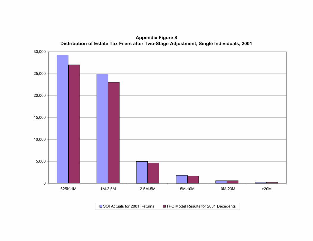
Appendix Figure 8Distribution of Estate Tax Filers after Two-Stage Adjustment, Single Individuals, 2001

0

5,000

10,000

15,000

20,000

25,000

30,000

625K-1M 1M-2.5M 2.5M-5M 5M-10M 10M-20M >20M


Appendix Figure 9Distribution of Gross Estate after Two-Stage Adjustment, Married Individuals, 2001

0

5,000,000

10,000,000

15,000,000

20,000,000

25,000,000

30,000,000

35,000,000

625K-1M 1M-2.5M 2.5M-5M 5M-10M 10M-20M >20M


Appendix Figure 10Distribution of Estate Tax Filers after Two-Stage Adjustment, Married Individuals, 2001

0

5,000

10,000

15,000

20,000

25,000

625K-1M 1M-2.5M 2.5M-5M 5M-10M 10M-20M >20M


Appendix Figure 11Distribution of Gross Estate after Two-Stage Adjustment, All Estate Tax Returns, Predicted

2001 Decedents vs. Actual 2002 Returns Filed

0

10,000,000

20,000,000

30,000,000

40,000,000

50,000,000

60,000,000

70,000,000

625K-1M 1M-2.5M 2.5M-5M 5M-10M 10M-20M >20M


Appendix Figure 12Distribution of Estate Tax Filers after Two-Stage Adjustment, All Estate Tax Returns,

Predicted 2001 Decedents vs. Actual 2002 Returns Filed

0

5,000

10,000

15,000

20,000

25,000

30,000

35,000

40,000

45,000

50,000

625K-1M 1M-2.5M 2.5M-5M 5M-10M 10M-20M >20M


Appendix Figure 13Net Estate Tax

0

1,000,000

2,000,000

3,000,000

4,000,000

5,000,000

6,000,000

< 1M 1M-2.5M 2.5M-5M 5M-10M 10M-20M > 20M

Size of Gross Estate

Net

Est

ate

Tax

($ th

ousa

nds)

2001 Decedents from TPC Model Returns Filed in 2001 From SOI Returns Filed in 2002 From SOI

Documents

The Urban-Brookings Tax Policy Center Microsimulation Model