THE UNIVERSITY OF CHICAGO RECOVERING EXPECTATIONS …charvey/Research/Thesis/Thesis.pdfthe university of chicago recovering expectations of consumption growth from an equilibrium model

THE UNIVERSITY OF CHICAGO

RECOVERING EXPECTATIONS OF CONSUMPTION GROWTH

FROM AN EQUILIBRIUM MODEL OF THE

TERM STRUCTURE OF INTEREST RATES

A DISSERTATION SUBMITTED TO

THE FACULTY OF THE GRADUATE SCHOOL OF BUSINESS

IN CANDIDACY FOR THE DEGREE OF

DOCTOR OF PHILOSOPHY

BY

CAMPBELL R. HARVEY

CHICAGO, ILLINOIS

DECEMBER, 1986

1

ACKNOWLEDGEMENTS

This research is supported by the Graduate School of Business and the Center forResearch in Security Prices at the University of Chicago and the Social Sciencesand Humanities Research Council of Canada. I have benefited from the commentsof my dissertation committee: Eugene Fama (Chairman), Wayne Ferson, RobStambaugh (inside members) and Lars Hansen, Shmuel Kandel, Merton Miller(outside members). I have also received valuable suggestions from Edward Allen,Daniel Beneish and Charles Kahn and from the Finance workshops at Carnegie–Mellon, Chicago, Cornell, Duke, M.I.T., Ohio State, Toronto, UCLA, Universityof Washington, Vanderbilt, Washington University, Wharton, and York. I amespecially indebted to Eugene Fama for his help with this project. The usualdisclaimer applies.

ii

1

TABLE OF CONTENTS

ACKNOWLEDGEMENTS . . . . . . . . . . . . . . . . . . . . . . . . . . . . . . . . . . . . . . . . . . . . . . . . . . ii

LIST OF FIGURES . . . . . . . . . . . . . . . . . . . . . . . . . . . . . . . . . . . . . . . . . . . . . . . . . . . . . . . . . iv

LIST OF TABLES . . . . . . . . . . . . . . . . . . . . . . . . . . . . . . . . . . . . . . . . . . . . . . . . . . . . . . . . . . vi

Chapter

1. INTRODUCTION . . . . . . . . . . . . . . . . . . . . . . . . . . . . . . . . . . . . . . . . . . . . . . . . . 1

2. MACROECONOMIC INFORMATION IN BOND PRICES . . . . . . . . . .3

2.1 The Consumer’s Planning Problem2.2 The Linear Specification2.3 The Generalized Method of Moments Approach2.4 Real Interest Rates and Yield Spreads

3. DATA SOURCES . . . . . . . . . . . . . . . . . . . . . . . . . . . . . . . . . . . . . . . . . . . . . . . . . 14

4. THE EMPIRICAL RESULTS . . . . . . . . . . . . . . . . . . . . . . . . . . . . . . . . . . . . . 17

4.1 Estimating Expected Inflation4.2 The Real Interest Rates and Yield Spreads

–Preliminary Data Analysis4.3 The Regression Results: Linear Specification4.4 Generalized Method of Moments Estimation:

Non-Linear Specification4.5 Alternative Predictors of Consumption Growth

5. CONCLUSIONS . . . . . . . . . . . . . . . . . . . . . . . . . . . . . . . . . . . . . . . . . . . . . . . . . . 86

Appendix

A. The Consumer’s Planning Problem: A More Detailed Examination . 88

B. The GMM Weighting Matrix . . . . . . . . . . . . . . . . . . . . . . . . . . . . . . . . . . . . . . 91

C. Data Sources and Definitions . . . . . . . . . . . . . . . . . . . . . . . . . . . . . . . . . . . . . .93

D. Supplementary Tables . . . . . . . . . . . . . . . . . . . . . . . . . . . . . . . . . . . . . . . . . . . . 104

E. Supplementary Figures . . . . . . . . . . . . . . . . . . . . . . . . . . . . . . . . . . . . . . . . . . . 112

REFERENCES . . . . . . . . . . . . . . . . . . . . . . . . . . . . . . . . . . . . . . . . . . . . . . . . . . . . . . . . . . . . 121

iii

1

LIST OF TABLES

1. Estimates of the Inflation Forecasting EquationsFull Sample Estimates . . . . . . . . . . . . . . . . . . . . . . . . . . . . . . . . . . . . . . . . . . . . . . . . 20

2. Evaluation of Inflation ForecastsOut-of-Sample j–Step Ahead Forecasts: 1953:2–1985:3 . . . . . . . . . . . . . . . . .26

3. Preliminary Data Analysis: Quarterly Data: 1953:2–1985:3Average Real Interest Rates and Real Consumption Growth . . . . . . . . . . .34

4. Preliminary Data Analysis: Quarterly Data: 1953:2–1985:3Average Yield Spreads and Real Consumption Growth . . . . . . . . . . . . . . . . 35

5. Preliminary Data Analysis: Annual Data: 1900–1984Average Real Interest Rates, Yield Spreads andReal Consumption Growth . . . . . . . . . . . . . . . . . . . . . . . . . . . . . . . . . . . . . . . . . . . 41

6. Ordinary Least Squares Estimation: Linear SpecificationAverage Interest Rates: Quarterly Data: 1953:2–1985:3 . . . . . . . . . . . . . . . 47

7. Generalized Method of Moments Estimation: Linear SpecificationAverage Real Interest Rates: Quarterly Data: 1953:2–1985:3 . . . . . . . . . . 48

8. Ordinary Least Squares Estimation: Linear SpecificationAverage Yield Spreads: Quarterly Data: 1953:2–1985:3 . . . . . . . . . . . . . . . .50

9. Generalized Method of Moments Estimation: Linear SpecificationAverage Real Yield Spreads: Quarterly Data: 1953:2–1985:3 . . . . . . . . . . 51

10. Ordinary Least Squares Estimation: Linear SpecificationAverage Interest Rates: Annual Data: 1900–1984 . . . . . . . . . . . . . . . . . . . . . 54

11. Generalized Method of Moments Estimation: Linear SpecificationAverage Real Interest Rates: Annual Data: 1900–1984 . . . . . . . . . . . . . . . . 55

12. Ordinary Least Squares Estimation: Linear SpecificationAverage Yield Spreads: Annual Data: 1900–1984 . . . . . . . . . . . . . . . . . . . . . .56

vi

LIST OF TABLES (continued)

13. Generalized Method of Moments Estimation: Linear SpecificationAverage Real Yield Spreads: Annual Data: 1900–1984 . . . . . . . . . . . . . . . . 57

14. Generalized Method of Moments Estimation: Non-Linear SpecificationAverage Real Interest Rates: Quarterly Data: 1953:4–1985:3 . . . . . . . . . . 64

15. Generalized Method of Moments Estimation: Non-Linear SpecificationAverage Real Interest Rates: Annual Data: 1900–1984 . . . . . . . . . . . . . . . . 66

16. Alternative Predictors of Consumption Growth:Lagged Consumption and Real Stock ReturnsQuarterly Data: 1953:2–1985:3 . . . . . . . . . . . . . . . . . . . . . . . . . . . . . . . . . . . . . . . .70

17. Alternative Predictors of Consumption Growth:Lagged Consumption and Real Stock ReturnsQuarterly Data: 1953:2–1985:3 . . . . . . . . . . . . . . . . . . . . . . . . . . . . . . . . . . . . . . . .71

18. Comparison of Forecasts: Interest Rate Model vs.Alternative Models Quarterly Data: 1953:2–1985:3 . . . . . . . . . . . . . . . . . . . . 72

19 Comparison of Forecasts: Yield Spread Model vs.Alternative Models Quarterly Data 1953:2–1985:3 . . . . . . . . . . . . . . . . . . . . . 72

20. Alternative Predictors of Consumption Growth:Lagged Cons. and Real Stock Returns: Annual Data: 1900–1984 . . . . . . 75

21 Comparison of Forecasts: Interest Rate Model vs.Alternative Models Annual Data: 1900–1984 . . . . . . . . . . . . . . . . . . . . . . . . . . 76

22. Comparison of Forecasts: Yield Spread Model vs.Alternative Models Annual Data: 1900–1984 . . . . . . . . . . . . . . . . . . . . . . . . . . 77

23. Evaluation of of Out-of-Sample Forecasting Performance:Quarterly and Annual Consumption Growth Forecasting Models . . . . . . 79

24 Comparison of Out-of-Sample Forecasting Performancewith the Commercial Macroeconomic Forecasting Services . . . . . . . . . . . . .85

vii

LIST OF TABLES (continued)

25. Preliminary Data Analysis: Quarterly Data: 1953:2–1985:3Spot Real Interest Rates and Consumption Growth . . . . . . . . . . . . . . . . . . . 105

26. Preliminary Data Analysis: Quarterly Data: 1953:2–1985:3Spot Real Yield Spreads and Real Consumption Growth . . . . . . . . . . . . . . 106

27. Normality Tests: Quarterly Data: 1953:2–1985:3Average Real Interest Rates and Real Consumption Growth . . . . . . . . . . .107

28. Normality Tests: Quarterly Data: 1953:2–1985:3Spot Real Interest Rates and Consumption Growth . . . . . . . . . . . . . . . . . . . 108

29. Normality Tests: Quarterly Data: 1953:2–1985:3Average Yield Spreads and Real Consumption Growth . . . . . . . . . . . . . . . . 109

30. Normality Tests: Quarterly Data: 1953:2–1985:3Spot Yield Spreads and Real Consumption Growth . . . . . . . . . . . . . . . . . . . 110

31. Normality Tests: Annual Data: 1900–1984Average Real Interest Rates, Yield Spreads andReal Consumption Growth . . . . . . . . . . . . . . . . . . . . . . . . . . . . . . . . . . . . . . . . . . . 111

viii

1

LIST OF FIGURES

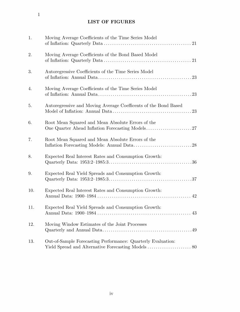
1. Moving Average Coefficients of the Time Series Modelof Inflation: Quarterly Data . . . . . . . . . . . . . . . . . . . . . . . . . . . . . . . . . . . . . . . . . . 21

2. Moving Average Coefficients of the Bond Based Modelof Inflation: Quarterly Data . . . . . . . . . . . . . . . . . . . . . . . . . . . . . . . . . . . . . . . . . . 21

3. Autoregressive Coefficients of the Time Series Modelof Inflation: Annual Data . . . . . . . . . . . . . . . . . . . . . . . . . . . . . . . . . . . . . . . . . . . . .23

4. Moving Average Coefficients of the Time Series Modelof Inflation: Annual Data . . . . . . . . . . . . . . . . . . . . . . . . . . . . . . . . . . . . . . . . . . . . .23

5. Autoregressive and Moving Average Coefficents of the Bond BasedModel of Inflation: Annual Data . . . . . . . . . . . . . . . . . . . . . . . . . . . . . . . . . . . . . . 23

6. Root Mean Squared and Mean Absolute Errors of theOne Quarter Ahead Inflation Forecasting Models . . . . . . . . . . . . . . . . . . . . . .27

7. Root Mean Squared and Mean Absolute Errors of theInflation Forecasting Models: Annual Data . . . . . . . . . . . . . . . . . . . . . . . . . . . .28

8. Expected Real Interest Rates and Consumption Growth:Quarterly Data: 1953:2–1985:3 . . . . . . . . . . . . . . . . . . . . . . . . . . . . . . . . . . . . . . . .36

9. Expected Real Yield Spreads and Consumption Growth:Quarterly Data: 1953:2–1985:3 . . . . . . . . . . . . . . . . . . . . . . . . . . . . . . . . . . . . . . . .37

10. Expected Real Interest Rates and Consumption Growth:Annual Data: 1900–1984 . . . . . . . . . . . . . . . . . . . . . . . . . . . . . . . . . . . . . . . . . . . . . 42

11. Expected Real Yield Spreads and Consumption Growth:Annual Data: 1900–1984 . . . . . . . . . . . . . . . . . . . . . . . . . . . . . . . . . . . . . . . . . . . . . 43

12. Moving Window Estimates of the Joint ProcessesQuarterly and Annual Data . . . . . . . . . . . . . . . . . . . . . . . . . . . . . . . . . . . . . . . . . . .49

13. Out-of-Sample Forecasting Performance: Quarterly Evaluation:Yield Spread and Alternative Forecasting Models . . . . . . . . . . . . . . . . . . . . . 80

iv

LIST OF FIGURES (continued)

14. Out-of-Sample Forecasting Performance: Annual EvaluationYield Spread and Alternative Forecasting Models . . . . . . . . . . . . . . . . . . . . . 81

15. Actual and Absolute Forecast Errors of the One QuarterInflation Forecasting Models . . . . . . . . . . . . . . . . . . . . . . . . . . . . . . . . . . . . . . . . . . 113

16. Root Mean Squared and Mean Absolute Errors of theTwo Quarter Ahead Inflation Forecasting Models . . . . . . . . . . . . . . . . . . . . . 114

17. Root Mean Squared and Mean Absolute Errors of theThree Quarter Ahead Inflation Forecasting Models . . . . . . . . . . . . . . . . . . . . 115

18. Root Mean Squared and Mean Absolute Errors of theFour Quarter Ahead Inflation Forecasting Models . . . . . . . . . . . . . . . . . . . . . 116

19. Actual and Forecasted Inflation: Time Series andTime Series Window Models: Quarterly Data . . . . . . . . . . . . . . . . . . . . . . . . . 117

20. Actual and Forecasted Inflation: Treasury Bill (Avg.) andTreasury Bill (Spot): Quarterly Data . . . . . . . . . . . . . . . . . . . . . . . . . . . . . . . . . 118

21. Actual and Forecasted Inflation: Time Series andTime Series Window Models: Annual Data . . . . . . . . . . . . . . . . . . . . . . . . . . . 119

22. Actual and Forecasted Inflation: Bond Based andRandom Walk Models: Annual Data . . . . . . . . . . . . . . . . . . . . . . . . . . . . . . . . . .120

v

CHAPTER 1

INTRODUCTION

In 1907, Irving Fisher proposed a consumption-based theory of interest rates.

Fisher suggested that, in equilibrium, the one year interest rate would reflect the

marginal value of income today relative to the marginal value of income next year.

The intuition is straight-forward. If a recession is expected next year, then there

is an incentive to sacrifice today to buy a one year bond that pays off in the

bad times. The demand for the bond will bid up the price and lower the yield.

The theory implies that there is information in current real interest rates about

expected economic growth.

This paper tests whether there is information in the term structure of inter-

est rates that is relevant for forecasting economic growth. The consumption-based

asset pricing framework refined by Rubinstein (1974, 1976), Breeden and Litzen-

berger (1978) and Lucas (1978) provides a set of first-order conditions that relate

marginal rates of substitution to asset returns. The first-order conditions are ma-

nipulated to express the expected marginal rates of substitution as functions of

real interest rates of various maturities. With a convenient utility specification,

real interest rates can be linked to expected real aggregate consumption growth.

Two types of interest rate variables are studied. The first is the real rate

of interest for various maturities. This measure is linked to consumption growth

rates over the same maturity. Second, the spread between annualized real rates – a

1

common measure of the term structure – is also examined. This variable is linked

to one-step ahead growth in consumption. The empirical analysis documents

the time series behavior of these interest rate variables. While the real interest

rates do not appear to be strong predictors of real consumption growth, the yield

spread variable has some predictive power – especially over the final 20 years of

the sample. The variable out-performs lagged consumption and real stock returns

in predicting economic growth within-sample and out-of-sample. Some evidence

is also presented that suggests that the spread specification forecasts have more

information than the forecasts of the commercial macroeconometric models.

The paper is organized as follows. Chapter 2 presents the framework whereby

expectations of consumption growth can be recovered. Chapter 3 documents the

data sources. The empirical tests are presented in chapter 4. Chapter 5 offers

some concluding remarks.

2

CHAPTER 2

MACROECONOMIC INFORMATION IN BOND PRICES

This chapter constructs the programming framework necessary to build an

equilibrium model of the term structure of interest rates. The well-known first-

order conditions are inverted to recover information about aggregate real consump-

tion growth from real bond yields. Two econometric methodologies are proposed

to deal with the separation of the interest rate and consumption variables. The

first method, suggested by Hansen and Singleton (1983), involves making strong

assumptions on the distribution of the joint consumption and returns process.

With these assumptions, the parameters can be estimated linearly. The second

strategy developed by Hansen (1982) and Hansen and Singleton (1982) involves

weaker assumptions and allows for consistent estimates of the parameters of the

non-linear first-order conditions with the Generalized Method of Moments (GMM)

technique.

2.1 The Consumer’s Planning Problem

Consider a pure exchange economy with a representative agent with additively

separable utility receiving a stochastic endowment. This agent can choose to

consume this endowment or invest in a portfolio of j–period bonds, {Bj,t : j =

1, . . . , k}. The bonds are assumed to be default free. Expectations at time t are

conditioned on the information set Ft – which contains all the information about

3

the environment available at time t. Consumption Ct is required to be measurable

at t with respect to Ft. The consumer maximizes the following objective:

max{Ct,Bj,t}∞

t=0 j=1,...,k

∞∑

t=0

δtE0U(Ct); 0 < δ < 1,

subject to:

CNt +

k∑

j=1

Bj,t ≤ Y Nt +

k∑

j=1

Bj,t−j(1 + RNj,t−j), (2.1)

where Ct is the agent’s real consumption, CNt represents nominal consumption,

RNj,t−j is the nominal yield on a j–period bond bought at time t− j, Et is the ex-

pectation operator conditioned on information Ft, Y Nt is the nominal endowment1

and δ is the consumer’s constant time discount factor. The first-order necessary

conditions2 are:

E

[δj U ′(Ct+j)

U ′(Ct)(1 + Rj,t) − 1

∣∣∣∣ Ft

]= 0, for j = 1, . . . , k, (2.2)

where Rj,t represents the real yield on a j–period bond. To keep the consumer’s

problem well behaved, the arbitrary rolling over of debt is ruled out. This effec-

tively imposes a limitation on the terminal value of the consumer’s debt holding.

Condition (2.2) is necessary to characterize an optimal plan. The Euler equation

(2.2) provides the basis for the intertemporal consumption-based asset pricing

model. Sufficient conditions are given in Rubinstein (1976), Breeden and Litzen-

berger (1978), Lucas (1978), Brock (1982) and Breeden (1986).1 The conditional expectation Et[Y N

t+j ] is assumed to exist for all j ≥ 1.2 See appendix A for a more detailed discussion of the problem and solution.

4

Equation (2.2) depicts a non-linear relation between the marginal rate of sub-

stitution and interest rates. Note that the real interest rate, Rj,t, represents the

total return over the period t to t + j. If this value is known at time t and the

parameterization of the utility function is also known, then it is possible to solve

for the expected marginal rate of substitution. Under some utility specifications,

the marginal rate of substitution can be linked to the growth rate in consump-

tion. With this type of specification, the real interest rate should forecast future

economic growth.

In practice, the real interest rate is not known at time t. The idea of this paper

is to look at expected real interest rates and to test if they contain information

about future growth in the economy. The next two sections outline methodologies

that allow for the estimation of consumption forecasting equations.

5

2.2 The Linear Specification

Let utility be represented by the constant relative risk aversion or isoelastic

class:3

U(C, α) =

{C1−α−1

1−α, if α > 0, α 6= 1;

log(C), if α = 1.(2.3)

With this convenient form, we can rewrite the initial first–order conditions as:

Et

[δj

{Ct

Ct+j

}α

(1 + Rj,t)]

= 1 j = 1, . . . k. (2.4)

Following Hansen and Singleton (1983), suppose that the process that charac-

terizes the marginal rates of substitution and the returns is stationary jointly

lognormally distributed. Then (2.4) can be re-written:

log Et

[δj

{Ct

Ct+j

}α

(1 + Rj,t)]

= Et log[δj

{Ct

Ct+j

}α

(1 + Rj,t)]

+

12vart log

[δj

{Ct

Ct+j

}α

(1 + Rj,t)]

= 0.

(2.5)

The RHS of (2.5) can be rearranged to bring expected consumption growth to the

LHS.

Et

[log

Ct+j

Ct

]=

j

αlog δ +

vj

2α+

1α

Et [log(1 + Rj,t)] , (2.6)

where vj is the variance term in (2.5) which is assumed constant. Equation (2.6)

is be estimated by least squares in the form:

3 The empirical section also considers negative exponential utility which impliesconstant absolute risk aversion.

6

logCt+j

Ct= βj

0 + β1Et [log (1 + Rj,t)] + εj,t+j . (2.7)

The coefficients should equal

βj0 =

j

αlog δ +

vj

2α,

β1 =1α

.

The β1 coefficient can be considered an elasticity as well as one over the relative

risk aversion. In the Life Cycle–Permanent Income Hypothesis literature, this

coefficient is sometimes referred to as the elasticity of intertemporal substitution. It

can be interpreted as the sensitivity of consumption growth to changes in expected

real rates. Recently, Hall (1985) has argued that this elasticity is very small and

perhaps even zero. This implies that there is no information in the expected real

rate that is relevant for forecasting real consumption growth. This paper will

provide an alternate way of estimating the inverse of the risk aversion parameter

or the elasticity of substitution by looking at the term structure rather than a

single short term interest rate. Evidence is presented that suggests that there is

some information in the term structure that is useful in forecasting consumption

growth.

Note that the least squares specification contains an expected value for a re-

gressor. A generated regressor will often lead to an errors in the variables problem.

This problem is usually addressed by using an instrumental variables technique.

The generated regressor vanishes if β1 is assumed to be unity (logarithmic util-

ity). It is immediate that expected inflation will cancel from both sides of equation

(2.7). Since the nominal rate is known at the beginning of the period, the expec-

tation operator can be dropped. The empirical section documents the results of

7

both the ordinary least squares regressions and instrumental variables estimation

for the case of an unrestricted coefficient of relative risk aversion. Results are also

presented for case where logarithmic utility is assumed.

If j > 1, then the error process {εj,t+j : t ≥ 1} will not be, in general, indepen-

dently distributed due to an overlapping dependent variable. The standard errors

on the regression coefficients need to be corrected for an induced moving average

process in the residuals. Following Hansen (1982) and White (1980), all stan-

dard errors are corrected for the moving average process and are heteroskedastic

consistent. 4

2.3 The Generalized Method of Moments Approach5

While the assumption of joint lognormality for the consumption-returns pro-

cess provides a simple way to obtain a consumption forecasting equation, it places

a strong restriction on the behavior of the data that may not be realistic. If the as-

sumption is violated, the parameter estimates will not be consistent. This causes

obvious problems in obtaining forecasts. Hansen’s (1982) Generalized Method of

Moments (GMM) technique allows for the consistent estimation of the parameters

of the first-order conditions with far weaker assumptions.

The GMM serves three uses here. First, the GMM based parameter esti-

mates can be compared to the linear estimates. If the assumptions of the linear

specification are true, then the two techniques should deliver the same parameter

4 Although the theory implies homoskedasticity, the use of heteroskedastic con-sistent variance-covariance matrix should not over turn any of the large sampleresults.

5 For a detailed description of this technique see Hansen (1982) and Hansenand Singleton (1982).

8

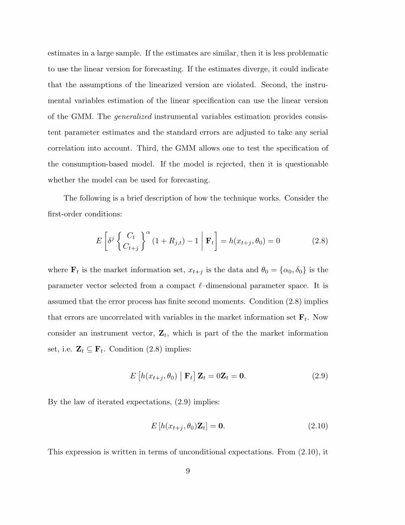
estimates in a large sample. If the estimates are similar, then it is less problematic

to use the linear version for forecasting. If the estimates diverge, it could indicate

that the assumptions of the linearized version are violated. Second, the instru-

mental variables estimation of the linear specification can use the linear version

of the GMM. The generalized instrumental variables estimation provides consis-

tent parameter estimates and the standard errors are adjusted to take any serial

correlation into account. Third, the GMM allows one to test the specification of

the consumption-based model. If the model is rejected, then it is questionable

whether the model can be used for forecasting.

The following is a brief description of how the technique works. Consider the

first-order conditions:

E

[δj

{Ct

Ct+j

}α

(1 + Rj,t) − 1∣∣∣∣ Ft

]= h(xt+j , θ0) = 0 (2.8)

where Ft is the market information set, xt+j is the data and θ0 = {α0, δ0} is the

parameter vector selected from a compact `–dimensional parameter space. It is

assumed that the error process has finite second moments. Condition (2.8) implies

that errors are uncorrelated with variables in the market information set Ft. Now

consider an instrument vector, Zt, which is part of the the market information

set, i.e. Zt ⊆ Ft. Condition (2.8) implies:

E[h(xt+j , θ0)

∣∣ Ft

]Zt = 0Zt = 0. (2.9)

By the law of iterated expectations, (2.9) implies:

E [h(xt+j , θ0)Zt] = 0. (2.10)

This expression is written in terms of unconditional expectations. From (2.10), it

9

is possible to construct an estimator of θ0 as long as the number of orthogonality

conditions (instruments), r, is greater than or equal to the number of parameters

to be estimated, `.

Let

G0(θ) = E [h(xt+j , θ)Zt] . (2.11)

Note that G0(θ) has a zero at θ = θ0. The method of moments estimator for G0

is:

GT (θ) =1T

T∑

t=1

h(xt+j , θ)Zt. (2.12)

At θ = θ0, GT (θ0) should be close to zero as T gets large. Equation (2.12) provides

the foundation for the GMM technique. The objective is to search for parameters

that force (2.12) to be as close as possible to the zero vector. The parameter

vector θT is chosen by minimizing the quadratic form:

JT (θ) = GT (θ)′WT GT (θ), (2.13)

where WT is a symmetric non-singular weighting matrix that defines the metric

used to make GT as close to zero as possible. Hansen (1982) shows that if, among

other assumptions, the parameter space is compact, ∂h∂θ is continuous and the

stochastic process {(xt+j , zt) : t ≥ 1} is stationary and ergodic, then the weighting

matrix, WT , will almost surely converge to a constant, W0. This implies that

θT will almost surely converge to θ0. This guarantees strong consistency and

asymptotic normality of the estimator.

If j = 1, then the r × r weighting matrix is computed by estimating:

10

W∗T =

[T∑

t=1

[h(xt+1, θT )Zt)][h(xt+1, θT )Zt]′]−1

. (2.14)

If j > 1, then the error process will be serially correlated. Appendix B demon-

strates how to construct the weighting matrix in this case. Note that an estimate

of θT is necessary in order to solve for W ∗T . The standard estimation strategy

proceeds in two stages. First, a sub-optimal choice of WT , such as the identity

matrix, is used in the minimization of the objective function (2.13). As a result

of this minimization, an initial parameter vector θT obtains. In the second stage,

the initial parameter vector is used to solve for the optimal weighting matrix, W ∗T

in (2.14). This matrix is used in the objective function and the final parameter

vector θ∗T is solved for.

The limiting variance-covariance matrix of the GMM estimator is consistently

estimated by:

Σ∗T =

{

1T

T∑

t=1

[∂h(xt+1, θ

∗T )

∂θ∗TZt

]}W∗

T

{1T

T∑

t=1

[∂h(xt+1, θ

∗T )

∂θ∗TZt

]}′−1

.

(2.15)

Furthermore, the number of observations times the minimized value of the objec-

tive function in (2.13) is distributed χ2 with r − ` (the number of orthogonality

conditions less the number of parameters) degrees of freedom. This statistic pro-

vides a test of the over-identifying restrictions7 in (2.12).

There are a number of advantages in using the GMM procedure to estimate

the non-linear first-order conditions. The strong distributional assumption of sta-

tionary joint lognormality need not be made. The GMM only requires that process

7 Consistent estimates can be obtained with the r = `. If r > `, then there arer − ` over-identifying restrictions that can be tested.

11

{(xt+j , zt) : t ≥ 1} be stationary and ergodic. The linear representation forces

the conditional covariance between returns and marginal rates of substitution to

be constant through time. The GMM does not impose this restriction. Finally,

the error process can be allowed to be conditionally heteroskedastistic. It is not

necessary to characterize the dependence of the conditional variances when using

the GMM technique.

2.4 Real Interest Rates and Yield Spreads

It is also of some interest to examine a measure of the term structure: the

spread between two annualized yields of different maturity. Kessel (1965) docu-

mented the cyclical nature of the term structure of interest rates. By subtract-

ing the one–period version of (2.6) from the j–period formulation, consumption

growth can be linked to the slope of the yield curve:

Et

[log

Ct+j

Ct+1

]=

j − 1α

log δ +vj − v1

2α+

1α

Et

[log

1 + Rj,t

(1 + R1,t)j

]+

j − 1α

Et [log(1 + R1,t)] .

(2.16)

This can be estimated in the form:

logCt+j

Ct+1= βj−1

0 + β1Et

[log

1 + Rj,t

(1 + R1,t)j

]+ β2Et [log 1 + R1,t] + εj−1,t+j . (2.17)

The coefficients should equal:

12

βj−10 =

j − 1α

log δ +vj − v1

2α,

β1 =1α

,

β2 =j − 1

α.

As with the interest rate specification, (2.17) contains generated regressors.

Both the expected yield spread and the expected real rate must be estimated. The

technique of instrumental variables is used for the estimation as well as ordinary

least squares. Note that with the assumption of logarithmic utility, the expected

inflation terms cancel from both sides of the equation and (2.17) can be estimated

in nominal terms.

There may be an advantage in using the yield spread specification. In the ex-

pected real interest rate formulation (2.7), the intercept contains vj . This variance

is assumed to be constant but in practice it may change through time. The spread

formulation (2.7) has the difference between vj and v1 in the intercept term. It is

possible that this difference is closer to a constant than the levels. The time series

behavior of the difference in the variances is investigated in the empirical section.

Two types of information available from bond prices are examined: real inter-

est rates and yield spreads. The intertemporal consumption-based asset pricing

model provides a framework whereby these financial variables can be linked to

macroeconomic fluctuations. Tests are conducted in chapter 4 to determine if

these variables have the explanatory power that the theory suggests.

13

CHAPTER 3

DATA SOURCES

The empirical analysis in this paper uses both quarterly and annual data.

The quarterly data span the 1953:2 to 1985:3 period. The annual data extend

from 1872 to 1984. A detailed discussion of each variable used is contained in

Appendix C. The following is a brief discussion of the data.

When calculating consumption growth, the National Income and Product

Accounts (NIPA) quarterly consumption data are used. These data incorporate

the 1985 revision in the National Accounts. The consumption data are in 1982

dollars and are seasonally adjusted1 by the Department of Commerce.

There are numerous problems associated with the NIPA consumption data.

Some of the components of consumption are omitted in the data collection. An-

other possible problem is the method of seasonal adjustment that the Bureau

uses. The Census Method II X–11 deseasonalizes by applying a series of centered

moving averages to the data. Unfortunately, important variation in the series may

be smoothed away. The method may also over-correct for seasonality. The data

1 When calculating the four quarter consumption growth, the not seasonallyadjusted consumption data are used. The X–11 seasonal adjustment program thatthe Department of Commerce applies a number of centered moving averages tothe data to extract the seasonal factors. These factors are allowed to vary throughtime. Hence, the annual rate of change in the seasonally adjusted data will notmatch the annual rate of change in the not seasonally adjusted data.

14

considered a proxy for true consumption. It is difficult to evaluate the quality of

the proxy.

The NIPA divide the consumption data into three categories: durables, non-

durables and services. The empirical work in the next sections uses the combined

measure of non-durables and services. All variables are transformed into per capita

terms with the Department of Commerce’s population estimate.

The consumption data represent average consumption over the quarter.2 If

consumption decisions were made once a quarter and on the first day of the quar-

ter, then it would be appropriate to use the interest rate for the first day of

the quarter. Since the consumption data represent average consumption over the

quarter, it seems more appropriate to use average interest rates in the analysis.3

In fact, the optimal averaging of the interest rate would exactly replicate the av-

eraging of the consumption data. Since it is extremely difficult disentangle the

consumption averaging process, simple averages have been imposed on the interest

rate data. To test the sensitivity of the empirical work to the use of the average

interest rate data, most of the results are replicated using spot interest rate data

for the last day of the first month of the quarter.4

The bill and bond data are obtained from the Selected Interest Rates and

2 Most of the Personal Consumption Expenditures on Non-Durables are sam-pled monthly from the Retail Trade Survey. Approximately 35% of the PersonalConsumption Expenditures on Services are sampled annually and trended, 5–10%of the Services are sampled quarterly and 55–60% of the data is sampled monthly.The quarterly consumption numbers are a sum of the monthly data. The measureis best thought of as average consumption over the quarter.

3 The averaging problem has been considered by Christiano (1984), Breeden,Gibbons and Litzenberger (1985), Grossman, Melino and Shiller (1985), Hall(1985) and Litzenberger and Ronn (1986).

4 Data for the second week of the second month of the quarter would be abetter mid-point but, unfortunately, these data were not available.

15

Bond Prices table of the Federal Reserve Bulletin. The data used are the yields

on three month, six month and nine month Treasury bills and yields on one year

Treasury bonds. The monthly data published by the Federal Reserve represent

the average of daily closing bid yields of at least five dealers. All bills are quoted

on a bank discount basis. The yields have been adjusted from bank discount to

true yield throughout the analysis. The quarterly yield data are the arithmetic

average of the monthly data. The spot interest rate data are an updated version

of the data used by Fama (1984a,b).

The annual data originate from a number of sources. The early consumption

data were collected by Kuznets (1961). As with the quarterly data, the annual

consumption variable is the sum of non-durables and services. The data span from

1871 to 1929 and are in 1929 dollars. The Department of Commerce’s consumption

estimates are used from 1929 to 1984. The data are spliced at the common year,

1929, and are converted into per capita measures by dividing by the Department

of Commerce’s population estimate.

The yield data are mainly from Homer (1963), Macaulay (1938) and the

Federal Reserve. A short-term interest rate is constructed by splicing yields on

New York City 30 to 60 day Commercial Paper (1900–1919) with yields on 90 day

Treasury bills (1920–1984). A longer term interest rate is constructed with a one

year corporate bond yield found in the Historical Statistics of the United States

(1900–1970) and some unpublished data from Scudder, Stevens and Clark (1971–

1984). Since the risk of the long term instrument is greater than the short term

instrument, a one year Treasury bond yield series is also used from 1953–1984.

16

CHAPTER 4

THE EMPIRICAL RESULTS

This chapter presents tests of some of the propositions developed in chapter

2. The consumption–based asset pricing model links expected real consumption

growth to expected real interest rates. At time t, only the nominal interest rates

are available. In order to calculate the expected real interest rates, a model of

expected inflation is necessary. The next section investigates the inflation process

and calculates expected real interest rates.

4.1 Estimating Expected Inflation

Three different inflation forecasting models are examined in this section. The

variable of interest is the rate of change in the price deflator for consumption of

non-durables and services. The simplest method presented is the random walk in

the inflation rate. Next a univariate time series representation is estimated for

the entire series and a moving sample window. Finally, the methodology of Fama

and Gibbons (1984) is used to calculate a Treasury bill based model of inflation.

Forecasts of inflation from t to t+1 for all of the models are based on information

available at time t. The parameters of each model are re-estimated at every point

in the series and the j–step ahead forecasts are calculated at every point.

17

4.1.1 Quarterly Data

The quarterly inflation process over the 1948:2–1985:2 period1 appears to

follow an IMA(1,1). An examination of the autocorrelogram shows a very slow

decay, a cut through the zero axis and a movement to significant negative values

at high orders. This type of structure is typical of mean non-stationary processes.

The other candidate process is an ARMA(1,1). This process is less likely to be the

correct process because of the shape of the autocorrelogram. When the models

are fit,2 the AR parameter of the mean reverting model is less than two standard

errors from one. The residual sum of squares of the IMA(1,1) and the ARMA(1,1)

are virtually the same – largely because of the closeness of the AR parameter to

one. This makes it difficult to choose the best model. A Dickey–Fuller unit root

test3 does not provide evidence against the null hypothesis of a unit root. The

IMA(1,1) is chosen on the basis of the initial identification. The estimates of the

IMA(1,1) model appear in table 1.

Inflation forecasts are obtained in two ways. First, the IMA(1,1) is estimated

over an initial period, 1948:2 to 1958:1. The fitted values provide the inflation

forecasts in this period. After this initial estimation period, the model is re-

estimated at each point in the time series and j–step ahead forecasts are obtained.

The second estimation strategy involves a moving sample window. After 1962:1,

1 There is data available for the 1946:2–1948:1 period. This part of the sampleis excluded because of the interventions in the time series that result from thelifting of war–time price controls.

2 All of the time series models are estimated with the exact likelihood algorithmavailable in the SCA computer package.

3 The Dickey–Fuller likelihood ratio test statistic for unit roots in series Yt iscalculated from H0 : (α, β, ρ) = (α, 0, 1) in Yt = α + β(time) + ρYt−1 + εt. Theyprovide an empirical distribution for the statistic in their 1981 paper. However,they admit that their test may lack power.

18

when a point is added to the sample, a point at the beginning of the sample

is dropped. The length of the window is 60 quarters.4 These estimates will be

referred to as Time Series Window. As with the first method, the parameters of

the model are re-estimated at every point in the time series. Figure 1 provides

graphs of the moving average parameter estimates over time. Plots of the actual

and fitted values from the two models are shown in the appendix.

The final model considered follows Fama and Gibbons (1984). In this repre-

sentation, a time series model is applied to the ex post real interest rate. Forecasts

are calculated and subtracted from the yield on a current Treasury bill to get an

implied measure of expected inflation. The identification of the time series model

for the real rate is similar to the exercise for the inflation rate. Two ex post real

rate series are considered: average rate on a 90 day Treasury bill over the quarter

and a spot rate in the middle month of the quarter. Both series are very similar.

The average series has a larger moving average component by construction. The

ex post real rate series appears to be mean non-stationary but the evidence is not

as clear as with the inflation rate.5 Again two models were fit: an IMA(1,1) and

an ARMA(1,1). The IMA(1,1) model was chosen. The estimates of the IMA(1,1)

parameters for the entire sample appear in table 1.

As with the time series model on the inflation rate, the univariate represen-

tation of the ex post real rate was estimated at each point in time after an initial

estimation period. Figure 2 shows how the moving average parameters of the

model applied to the spot and average data vary through time. As expected, the

4 The window is chosen to be long enough to allow the parameter values toexhibit some stability. If the window was shorter, say 20 quarters, the modelidentification might change as a result of a different location in the business cycle.

5 The Dickey-Fuller unit root test does not provide much evidence against thenull hypothesis of a unit root.

19

moving average parameter associated with the average interest rate data has a

higher value. But it is remarkable how similar the parameter sequences are. It is

also interesting to note the jump downward in the parameters in the 1973–1974

period and the 1979–1981 period. These periods coincide with recessions. The

decline in the value of the moving average parameters indicate that a greater pro-

portion of change in the real rate is unexpected. The inflation forecasts generated

from these models will be referred to as Treasury Bill (Avg.) and Treasury Bill

(Spot).

20

4.1.2 Annual Data

While annual inflation data exist from 1872–1984, the one-year yield series

is available only from 1900 to 1984. The time series based model of the inflation

rate uses the entire series but the forecasts are restricted to the 1900–1984 period.

The identification of the annual inflation process is more straight-forward

than the quarterly inflation process. The annual inflation rate appears to follow

an ARMA(1,1). Estimates of the parameters of this model for the full sample are

provided in table 1. One step ahead forecasts are generated by re-estimating the

parameters of the model at each point in the series starting in 1900. As with the

quarterly data, a time series window model is also estimated. The window length

is 20 years. This is a longer period than the quarterly model. It is difficult to

have much confidence in the time series estimates if fewer than 20 data points

are used. Forecasts are generated from 1900 to 1984. Figures 3 and 4 show the

time series behavior of the ARMA parameter estimates. The both the MA and

AR parameters on the time series model are fairly stable through the sample.

The time series window estimates track these parameters closely until 1950 after

which there is often a wide divergence between the windowed and unwindowed

estimates.6

The final model considered is a time series model for the ex post real rate.

In the 1900–1983 period, the realized real rate appears to follow an ARMA(1,1).

Since the sample size is smaller, the fitted values are used for forecasts in the

1900–1919 period. The model is re-estimated at every point in the time series

after 1919 and one-step ahead forecasts are obtained. The full sample estimates

of this model are provided in table 1. Figure 5 plots the estimates of the ARMA

6 This could be due to the small size of the window.

22

parameters through time. The parameter estimates are reasonably stable except

during the 1929–1934 period. In the depression, the AR parameter moves close

to one and the MA parameter drops toward zero. This suggests that the process

resembles a random walk in this particular sample. As in the quarterly sample,

during recessionary periods changes in the real rate appear to be unpredictable.

23

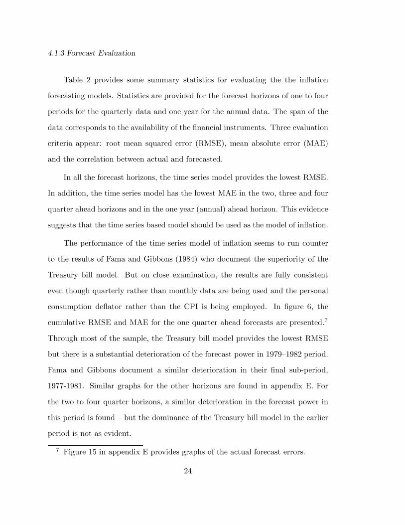
4.1.3 Forecast Evaluation

Table 2 provides some summary statistics for evaluating the the inflation

forecasting models. Statistics are provided for the forecast horizons of one to four

periods for the quarterly data and one year for the annual data. The span of the

data corresponds to the availability of the financial instruments. Three evaluation

criteria appear: root mean squared error (RMSE), mean absolute error (MAE)

and the correlation between actual and forecasted.

In all the forecast horizons, the time series model provides the lowest RMSE.

In addition, the time series model has the lowest MAE in the two, three and four

quarter ahead horizons and in the one year (annual) ahead horizon. This evidence

suggests that the time series based model should be used as the model of inflation.

The performance of the time series model of inflation seems to run counter

to the results of Fama and Gibbons (1984) who document the superiority of the

Treasury bill model. But on close examination, the results are fully consistent

even though quarterly rather than monthly data are being used and the personal

consumption deflator rather than the CPI is being employed. In figure 6, the

cumulative RMSE and MAE for the one quarter ahead forecasts are presented.7

Through most of the sample, the Treasury bill model provides the lowest RMSE

but there is a substantial deterioration of the forecast power in 1979–1982 period.

Fama and Gibbons document a similar deterioration in their final sub-period,

1977-1981. Similar graphs for the other horizons are found in appendix E. For

the two to four quarter horizons, a similar deterioration in the forecast power in

this period is found – but the dominance of the Treasury bill model in the earlier

period is not as evident.

7 Figure 15 in appendix E provides graphs of the actual forecast errors.

24

In figure 7, the cumulative RMSE and MAE for the annual forecasts are

presented. There is a large jump upwards in the forecasting errors in the time of

depression. The quarterly data exhibited jumps in the errors in the 1973–1975 and

1979–1982 periods. The annual data show a deterioration in the forecast power in

the 1929–1934 period but there is no deterioration in the 1970’s. The correlations

between actual and fitted are lower for the annual data indicating that it is more

difficult to forecast one year ahead. Finally, there is not much difference in the

forecasting power of the bond based model or the time series based model. In

the first 20 years of evaluation, the bond model does better than the time series

model. But this could be due to the fact that the bond model is using fitted values

during these years whereas the time series is using out-of-sample forecasts.

It is important to note that these models are just approximations of the

true expectations generating mechanism. There is no reason to presume that the

expectation generation process remains fixed through time. New variables may

enter the process and old variables may be dropped. Letting the parameters vary

through time may help the time series models adjust to this type of change in the

true underlying structure.

While the model evaluation seems to point to the time series representation

of inflation, many of the results are replicated using the alternative models of

expected inflation. This provides a test of how sensitive the results are to the use

of different expected inflation measures.

25

4.2 Real Interest Rates and Yield Spreads – Preliminary Data Analysis

The inflation forecasts in the previous section are now applied to the nominal

interest rate structure in order to calculate the expected real rates. The theory

suggests that expected real rates should be related to consumption growth. The

preliminary data analysis provides an informal way to assess the similarities and

differences in the time series. Tables 3–5 present some summary statistics for

quarterly and annual measures of real consumption growth, expected real interest

rates and yield spreads. These statistics are based on average nominal interest

rates. Tables 25 and 26 in appendix D replicate these statistics using the spot

interest rates for the quarterly data. These tables also provide preliminary data

analysis for the real rates calculated with different models of inflation: time series,

time series window, Treasury bill and random walk. The ex post real rate is also

included.


Summary statistics are provided in table 3 for the expected real rates and

growth in consumption of non-durables and services. The results of Working

(1960) show that the difference between two series that are averaged will induce

a first-order moving average process in the differenced series.8 If consumption

follows a geometric random walk, then the growth in consumption should follow

a moving-average process with a first-order autocorrelation coefficient of .25 and

higher order autocorrelation coefficients of zero. The results in table 3 show that

the sample first-order autocorrelation coefficient for the one quarter consumption

8 Both Hall (1985) and Breeden, Gibbons and Litzenberger (1985) have appliedthese results to the consumption data.

29

growth is .245 which is close to the hypothesized value but the higher order coeffi-

cients are not all close to zero. Since the consumption growth is a continuous–time

growth rate, the longer growth rates are just sums of the one-quarter rates. Hence,

the two to four quarter growth rates should follow two to four quarter moving-

average processes. Furthermore, the first-order serial correlation coefficient will

increase as more series are summed.9 This is more or less what is seen in table

3.10

An examination of the autocorrelogram of the real rate process reveals a

different picture. As mentioned earlier, the real rate process has a slow decay that

is either indicative of a non-stationary process or a mean reverting process with

an AR coefficient close to unity. The two to four quarter expected real rates are

not sums of the one quarter rate as was the case with consumption growth. An

across horizon comparison suggests that all of the expected interest rates have a

similar autocorrelation function.

Table 4 presents the preliminary data analysis for the expected real yield

spreads and real consumption growth. The consumption growth statistics are

again displayed on the top line of each panel. The expected j–period real yield

spread measure has a different time series behavior than the expected real interest

rates which are its components. The autocorrelograms of the three ex ante yield

spreads show a sharp decay to zero. The autocorrelation structure is roughly

similar to that of the consumption growth measures.

9 If ∆Ct = (1− θL)εt, where L is the lag operator, then the sum of n adjacentseries is

∑nj=1 ∆Ct+1−j = (1 −

∑n−1j=1 (θ − 1)Lj − θLn)εt. From this expression,

the autocorrelations of the summed series can be derived. For example, if in theMA(1) ρ1= .25, then MA(2):ρ1=.60, MA(3):ρ1=.77 and MA(4):ρ1=.82.

10 Note that the length of the series is different across horizons. Also, the fourquarter growth rates are not the sum of the one quarter growth rates. They arethe sum of the one quarter not seasonally adjusted growth rates.

30

The summary statistics suggest that the expected real rates are either mean

non-stationary or mean reverting with a high autoregressive coefficient yet the

spread and the consumption growth series are clearly mean stationary. This is not

necessarily inconsistent with the model. The growth in consumption should equal

the expected real rate plus noise. If noise is added to the expected interest rate

process, it should end up looking random like the consumption growth process.

A more detailed look at the quarterly data is presented in appendix tables

27–30. These tables present measures of skewness and kurtosis as well as two

normality test statistics. Given that the data are stationary, these test statistics

provide information about the distribution of the data. Two normality test statis-

tics are the studentized range and the Kolmogorov D–statistic.11 The D–statistics

show that we cannot reject at the one percent level of significance the null hy-

pothesis of normality for all of the consumption growth series and for the two and

three quarter yield spread series. There is evidence against the null hypothesis

with the other interest rate measures. Joint lognormality of the marginal rates of

substitution and the interest rate measures is important to the linear specifica-

tion of the model. The normality test results suggest that this assumption is not

supported by the data when applied to the real interest rates. But the assump-

tion is supported for the yield spread specification. Additional tests presented in

11 Order the sequence {xj : 1 ≤ j ≤ n} such that {x1 ≤ x2 ≤ . . . ≤ xn}. TheKolmogorov D–statistic is defined as D =

√n sup|Fn(x) − F (x)| where Fn(x) is

the observed cumulative distribution function and F (x) is the uniform cumulativedistribution. The D–statistic measures the greatest divergence between the twodistributions. Given a null hypothesis that the sequence is normally distributed, ahigh value (close to unity) provides evidence against the null hypothesis. However,the test assumes that {xj} are independently identically distributed random vari-ables. Some caution should be exercised when applying this test to a time series,such as consumption growth, where it is difficult to argue that the drawings arei.i.d.

31

section 4.3 suggest that these results could be due to a non-constant variance in

the expected real rate process. The variance in the expected yield spread process

is roughly constant.

Some of the data are displayed in figures 8 and 9. If the assumptions of the

linear specification are accurate, then the consumption growth series should look

like the expected interest rate series plus noise. If the noise component is small

then, the series should exhibit similar co-movement. Figure 8 shows the one to

four quarter consumption growth plotted against the one to four quarter real rate

(calculated with the time series model of inflation). The interest rate variables

are lagged to match the span of the consumption growth, i.e., a bill that has three

quarters to maturity at time t is matched with consumption growth from t to

t+3. If these series exactly coincide, then the expected real interest rate perfectly

forecasts future consumption growth. The plots show that the consumption series

have constant variances. However, the expected real interest rates appears to have

non-constant variances. Second, the consumption and interest rate series move

with similar long-term trends; both of the series would be quite similar if a high-

order moving average were applied to the data. Third, the interest rate deviates

sharply from the consumption growth series in the 1979–1982 period. This coin-

cides with the period when the Federal Reserve announced it was changing the

focus of its monetary policy. This period is characterized by large unprecedented

swings in interest rates.

The plots of the yield spread and consumption growth are presented in figure

9. There are a number of interesting features to these graphs. First, the variance

of the spread series seem more constant than the variance of the expected real

interest rate process. This is especially evident with the two and three quarter

32

spreads. Second, the deviation in 1979–1982 largely disappears. Third, in the

1964–1967 period, the spread measure is flat whereas there is some volatility in

the consumption measure. It is possible that consumers made forecasting errors

during this period or the inflation forecasting model used in the analysis does

not adequately capture consumers’ expectations. The fourth and perhaps most

striking point that is evident from figure 9 is the similarity in the movement of the

two series. Examination of the figure suggests that the yield spread may contain

information relevant for the forecasting of consumption growth.

33

4.2.2 Annual Data

Table 5 presents summary statistics for the annual data. The top panel of

this table considers the 1900–1984 period. The real interest rate variable is a

one year corporate bond yield. The spread variable is constructed by taking the

natural logarithm of the ratio of the one year corporate yield and the yield on

30–60 day Commercial paper (1900–1919) and 90 day Treasury Bills (1920–1984).

The second panel shows the annual data for the 1953–1984 period. The interest

rate variable in this sub-period is the rate on a one year government bond. The

spread is constructed with the yields on two government instruments. This sample

is the more reliable than the longer period because the government instruments

are available and because this sub-period follows the Treasury–Federal Reserve

Accord.

In the 1900–1984 period, the consumption growth variable appears to be mean

stationary with the autocorrelation function trailing off to zero by the third lag.

The first-order autocorrelation coefficient exceeds the .25 value that is expected

if the underlying series follows a geometric random walk. Caution should be

taken in interpreting this time series due to the splicing of the data in 1929. The

1900–1929 data are based on interpolated values from five year sampling intervals.

This induces a higher order moving average process in the early data and high

autocorrelations are expected. In the 1953–1984 sample, the sample first-order

autocorrelation coefficient is .251 which is more in line with the quarterly results.

While the autocorrelation function of the expected real rate in the 1900-1984

period presented in table 5 looks similar to the expected real rate in the quarterly

sample documented in table 3, the annual spread measure takes much longer to

decay to zero. This could be due to the splicing of instruments in the short

38

term yield series or due to the construction the spread as the difference between

a corporate bond and a government bill. The 1953–1984 sub-period is chosen

to avoid both of these problems and the autocorrelations are very similar to the

quarterly results.

A more detailed examination of these series is contained in appendix table 31.

The evidence suggests that the null hypothesis of normality cannot be rejected

at the one percent level of significance for the yield spread measure in the full

sample and the consumption growth measure in the 1953–1984 period. Normality

can be rejected for the real interest rate in both samples. These results may cause

problems with the linear specification – at least when it is tested using real interest

rates.

Graphs of the data appear in figures 10 and 11. As with the quarterly plots,

the data are arranged so that if the series exactly coincide, the interest rate variable

provides a perfect forecast of the growth in the economy. The one year growth in

consumption and the one year expected real interest rate for the 1900–1984 period

are plotted in figure 10. There is a large divergence in the two series during the

great depression. Consumption growth is low whereas the expected real yield on

the bond is high. The nominal yield on the bond is relatively low. During this time

there is a considerable deflation. The time series based forecasting model predicts

continued deflation. This leads to the high expected real yields. It is possible that

the true inflationary expectations are different during this period. Examination

of the inflation forecasting errors of the time series model show large errors in this

period. It is also possible that the real expected yields are high because the default

risk for the corporate bonds increases. The theory is presented in terms of default-

free instruments. The expected real rate roughly tracks the consumption growth

39

– especially after 1935. There is another large deviation after 1979. Figure 10 also

highlights the 1953–1984 period. The change after 1979 is particularly evident

in this figure. The deviation coincides with the Federal Reserve’s announcement

that it would change the focus of its monetary policy.

Plots of the yield spread measures are in figure 11. The divergence of the two

series during the depression is not as wide as seen with the expected real interest

rate. The expected spread series roughly moves with consumption growth through

much of the sample. The relation seems particularly strong after 1950. The graphs

suggest that there may be important information in the expected spread that could

be used to help forecast growth in consumption.

40

4.3 The Regression Results: Linear Specification

If the consumption-based model is an adequate description of the world and if

the joint distribution of the consumption growth and real rate series is stationary

lognormally distributed, then it may be possible to extract information about

future consumption growth from the real rate with linear least squares. The

preliminary data analysis indicates that we are less likely to find information in

individual interest rates. The summary statistics and the graphs suggest that the

spread specification better fits the assumptions of the linearized model.


The regression results in table 6 for expected real interest rates show that

the interest variables appear to have no power to explain variation in future con-

sumption growth. None of the coefficients on the interest rate variables are more

than one standard error from zero. All of the standard errors are corrected for

a moving average induced in the residuals as a result of overlapping dependent

variables. Standard errors are also adjusted for conditional heteroskedasticity.12

There may be econometric problems associated with these regressions. The

first is the errors in the variables problem. The expected real rate is forecasted

and subject to error. As a result, the parameter estimates could be inconsistent.

The second problem relates to the assumption of stationary joint lognormality. If

12 This procedure follows White (1980) and Hansen (1982). Let j be the or-der of the moving average process. Define SW = 1

T

∑ji=−j

∑Tt=1 u′

tut−iX′tXt−i,

where ut are the regression errors. The variance covariance matrix is then1T

(X ′X)−1S−1W (X ′X)−1 1

T. This matrix follows the variance covariance matrix

presented Theorem 1 of White (1980) if j = 0 and Theorem 3.1 of Hansen (1982)for the more general case of j ≥ 0.

44

this assumption is violated, then the regressions are not well specified.

The errors in the variables problem can be addressed with the use of instru-

mental variables estimation. Table 7 presents some results13 using a linear version

of the GMM technique of Hansen (1982). The instrumentation consists of a con-

stant, the expected real rate from a time series model14 on the realized real rate

and the log of the ratio of yields on Moody’s BAA and AAA rated bonds.15 The

instrumental variables are all important predictors of the realized real rate. The

GMM estimates of the risk aversion parameter are all positive but not different

from zero at conventional levels of significance. This contrasts with the negative

point estimates of the risk aversion parameter in two of the four interest rates

in the OLS results. The GMM estimation does not provide evidence against the

specification with one over-identifying restriction – but there does not seem to be

much explanatory power in the specification.

Figure 12 provides a plot of a three year moving window estimate of the

variances of joint processes. There is a large increase in the variance in the 1979–

1982 period. The linear specification assumes that the variance of the joint process

is constant and it is grouped into the intercept term for estimation. The plot of

the variance suggests that this assumption is violated. The graph suggests that

a closer approximation might be obtained by using the difference in the variance

of two processes. This is precisely what the yield spread specification groups into

the intercept term.

13 Estimates were obtained using a modified version of a GMM program writtenin GAUSS by David Runkle and Gregory Leonard.

14 Since the time series model is re-estimated at each point in time, this variableis predetermined and hence a legitimate instrument.

15 Keim and Stambaugh (1986) present evidence that this variable is able topredict excess bond returns.

45

The OLS estimates of the yield spread specification are presented in table

8. Following equation (2.17), both the expected yield spread and the level of the

short-term rate are included as explanatory variables. The full sample results

suggest that this specification has only marginal explanatory power: six percent

of the variation in the two quarter consumption growth is explained but none of

the variation in the one and three quarter consumption growth is explained. Some

sub-period results are also presented. The first sub–period (ending in 1971:4) is

similar to the overall period where there is only slight explanatory power. The

second sub-period shows a different picture. The three yield spreads can explain

3%, 23% and 24% of the variation in one to three quarter consumption growth.

The instrumental variables estimates for the full sample are presented in table

9. As with the GMM results in table 7, none of the parameters are significantly

different from zero. However, the point estimates are close to those delivered by

OLS. The OLS parameter estimates on the one to three quarter yield spread are

.28, .86 and .42 while the GMM estimates are .11, .76 and .21. As mentioned

earlier, if the estimates are fairly close, then it is less problematic to use the OLS

for prediction.

The regression results show that there is no power to predict consumption

growth when examining quarterly expected real interest rates. However, there is

some ability to predict consumption growth when the yield spread is combined

with the short term rate. The explanatory power seems to be concentrated in

the second sub-period. A possible explanation for the yield spread having more

predictive ability is a changing variance of the joint process. The yield spread

specification uses a difference in the variance while the interest rate specification

uses the level of the variance.

46

4.3.2 Annual Data

The results of the regression analysis of the real interest rate and annual

consumption growth are in table 10. Similar to the quarterly results, very little

information seems to be contained in the level of the real rate. The coefficient

on the real rate in the overall period is negative which is the opposite sign that

standard economic theory would predict. In the post-depression sample, the coef-

ficient is positive but the standard error is large. As with all the OLS regressions,

the standard errors are corrected for a first-order moving average process and for

conditional heteroskedasticity.

The GMM estimates presented in table 11 are similar to the OLS estimates.

This could indicate that the errors in the variables problem is not that severe in

the annual data. But there may be other problems with the linear specification.

Figure 12 presents a plot of five year moving window estimate of the variance

of the joint process for the annual data. There is a large jump in the variance in

the 1929–1934 period. This is possibly the reason that the interest rate series and

the consumption growth series widely diverge in this period.

Table 12 presents the results using the yield spread specification. In the

overall period, 1901–1984, neither of the coefficients are significantly different from

zero. In the post-depression sample, the yield spread enters with a coefficient that

is more than three standard errors from zero. Similarly, the yield spread enters

with a coefficient that is greater than two standard errors from zero in the post–

1953 sample. These results are corroborated by the GMM results presented in

Table 13. The point estimates on all the parameters are slightly larger. The

52

coefficients on the yield spread are positive and in the post-depression sample are

1.6 standard errors from zero.

The annual results suggest that the yield spread variable has some ability

to predict consumption growth – but this ability is limited. The real rate has

virtually no power to predict. The lack of power could be due to a number

of factors such as: errors in the variables, a non-constant variance of the joint

process, inflation forecasting errors, government interventions, the averaging of

the interest rates, the unavailability of a long-term government instrument before

1953 or a mis-specification of the underlying model. The evidence presented in

this section points to large inflation forecasting errors in the depression as well as

a non-constant variance as the likely culprits. The reason the spread specification

tends to do better is probably because it allows the variance to change through

time.

53

4.3.3 Nominal Interest Rates and Consumption Growth

Most of the econometric problems are caused by the need to estimate a real

rate of interest at time t for t to t + j. If the assumption of logarithmic utility

is maintained, then the first-order conditions can written in terms of nominal

rates of interest and nominal consumption growth. Since the j–period nominal

interest rate is in the information set at time t, the expectation operator can be

dropped from the regressor. Previous studies, such as Hansen and Singleton (1982,

1984), Ferson (1983), Brown and Gibbons (1985), Dunn and Singleton (1985), Hall

(1985), Mankiw (1985) and Miron (1985) could not reject a relative risk aversion

coefficient of unity.

The nominal specification reverses the steps of the real model. In the nominal

specification, the nominal rate is used to forecast nominal consumption growth.

The inflation forecasts are then subtracted from the fitted values in the nomi-

nal regression to provide forecasts of the growth rate in real consumption. The

advantage of this specification is the ability to avoid the errors in the variables

problem. Another advantage is that the assumption of joint lognormality of the

interest rate and consumption growth processes need not be made.

The results of the nominal specification for the quarterly data are provided in

tables 6 and 8. Two R2s are presented. The first is the coefficient of determination

resulting from the regression of nominal interest rates on nominal consumption

growth. The second R2 results from the regression of the fitted values of nominal

growth model less the inflation forecasts on real consumption growth. In the inter-

est rate specification, the nominal-based predictions do better than the expected

real predictions. Table 6 shows that the nominal-based model can explain 2–16%

of the variation in real consumption growth while the expected real rate can ex-

58

plain none. The nominal-based predictions also tend to do better in the overall

period in the yield spread specification. Table 8 shows that these predictions can

account for 5–14% of the variation in the real consumption growth. The nominal

based predictions also tend to do better in the first sub-period. The second sub-

period is characterized by similar predictive power for both the nominal-based

and the expected real-based.

The annual results are presented in tables 9 and 11. As with the quarterly

data, table 9 documents the nominal-based predictions consistently outperforming

the expected real interest rates in explaining real consumption growth. In the yield

spread formulation, the nominal-based and expected real models explain a similar

amount of the variation in the real consumption growth.

In addition to avoiding some of the errors in the variables problems, the

nominal-based predictions outperforming the expected real interest rate predic-

tions is consistent with the conjecture that the changing variance of the joint

process may be causing estimation problems. The nominal-based model does not

rely on the assumption of stationary joint lognormality of the real interest rate

and consumption growth. The dominance of the nominal-based predictions is not

as evident when looking at the yield spread specification. Sometimes the expected

yield spread has more power than the nominal-based predictions. This is consis-

tent with the conjecture that the yield spread specification minimizes the changing

variance problem by utilizing a difference in two variances.

4.4 GMM Estimation: Non-Linear Specification

59

This section presents results of the direct estimation of the first-order condi-

tions using the Generalized Method of Moments. This technique has been used

to estimate the linear version of the model. The advantage of the non-linear es-

timation is that the strong distribution assumptions necessary to linearize the

model need not be made. Unfortunately, the non-linear estimation does not pro-

vide forecasts. But we can learn something about the parameter values from this

estimation technique. If the assumptions of the linear version of the model are

true, then the non-linear estimation should deliver the same parameter estimates.

4.4.1 Quarterly GMM Estimation

The results of the generalized method of moments estimation of the non-linear

first-order conditions are in table 14. The instrumentation consists of a constant,

the expected real rate from a univariate time series model, lagged consumption

growth and the natural logarithm of the ratio of the yields on Moody’s BAA and

AAA rated bonds. The point values of the coefficient of relative risk aversion range

from .6 to 1.3 in the one to four quarter samples. However, the standard errors

are generally large. This range is fairly narrow compared to the values reported in

other studies.16 For example, using monthly data, Hansen and Singleton report

estimates from -1.3 to 1.6. The quarterly estimates in table 14 are always positive

16 Using monthly data, Brown and Gibbons (1985) estimate a range for thecoefficient of relative risk aversion of .09 to 7.00. Dunn and Singleton (1985)report values between 1.22 and 1.91 for the single equation estimation and 2.50to 3.45 for the multiple equation estimates. With quarterly consumption data,Mankiw, Rotemberg and Summers (1985) document values from .09 to .51 in thecase where utility is assumed to be separable between consumption and leisure.Mankiw (1985) reports a range between 2.43 and 5.26 using only the fourth quarterdata for each year. Using seasonally unadjusted data, Miron (1985) documents arange of .02 to 1.71 for the risk aversion parameter. All of these studies use theGMM technique to obtain parameter estimates.

60

– the sign predicted by economic theory.

The point estimates of the linear version of the model for real interest rates

range from 8.9 to 22.7 as reported in table 7. Again the standard errors are large.

The wide divergence from the non-linear estimates seems to suggest that the

linear version with real interest rates is mis-specified. The GMM results reported

in table 9 using the yield spread specification deliver estimates of 9.1, 1.3 and 4.5.

While these estimates are still high compared to the non-linear estimates, they

suggest that the yield spread specification may be superior to the interest rate

specification. If the true parameter of constant relative risk aversion does fall in

the range of .6 to 1.3, then only the yield spread regressions provide that range

for the coefficient – particularly in the 1972:1–1985:3 sub-period.

Table 14 also provides a test of the over-identifying restrictions. None of the

specifications is rejected at the .01 level of significance. The tests indicate that

there does not seem to be much evidence against the constant relative risk aver-

sion (CRRA) specification. Previous research has concentrated on single period

returns and the model has received mixed support. Hansen and Singleton (1984)

cannot reject the model when a single asset is used. However, they find evidence

against the model when more than one asset is used. Dunn and Singleton (1985)

using a formulation that allows for durable goods find similar results in testing

single equation versus multiple equation specifications. Mankiw, Rotemberg and

Summers (1985) find evidence against the model when they use the seasonally

adjusted quarterly data in both cases of separable and non-separable utility in

consumption and leisure. Yet when they re-estimate using only the fourth quar-

ter data, they do not reject the model. Mankiw’s (1985) specification allows for

durables as well as non-durables to be incorporated into the model. Using fourth

61

quarter data, he does not find evidence against the specification. Miron (1985)

uses seasonally unadjusted data and finds no evidence against the over-identifying

restrictions.

The results in Table 14 are not directly comparable to any of the above studies

because different asset return data are used and the model is often formulated

in different terms in other research, i.e., allowing for consumption services from

durables. The results in table 14 indicate that the strongest case against the

model can be made from the one quarter rate of change specification. There

is little evidence against the model when it is tested with longer term growth

rates. A possible explanation for this phenomena is measurement error in the

data. Suppose that the measured consumption data sometimes incorporate some

information from the next period. This could be caused by the retail sales data

collection being off by a few days or the trending of the services data (some

of which is collected semi-annually and annually). It could also be result from

the forward smoothing of the seasonal adjustment procedure. If this is the case,

the measured marginal rate of substitution and the asset return are improperly

matched in the first-order conditions and the lagged consumption growth is no

longer a valid instrument in the estimation. This is less of a problem when longer

term growth rates are used relative size of the error is smaller.

The measurement error explanation is consistent with the pattern of the χ2

statistics in table 14. The size of the test statistics decreases from the one to three

quarter models indicating that there is less evidence against the model as longer

growth rates are used. The four quarter growth model reported in table 14 is not

directly comparable to the one to three quarter models because the not seasonally

adjusted data is used in this case. The size of the measurement error is probably

62

smallest when the model is tested using the seasonally unadjusted data because

the series is not forward filtered. The results suggest that there is little evidence

against the four quarter specification.

For comparison, the same first-order condition is tested with negative expo-

nential utility17 which implies constant absolute risk aversion (CARA). In contrast

to the CRRA results, the CARA model is rejected at the .05 level in three of the

four maturities. These results suggests that the CRRA is a superior specification.

17 Ferson (1983) provides some tests of the model with a CARA specificationusing a maximum likelihood estimation technique. There are no studies that havetested the CARA model using the instrumental variables methodology.

63

4.4.2 Annual GMM Estimation

The generalized method of moments estimation of the non-linear first order

conditions is presented in table 15. The instrumentation consists of a constant,

the expected real rate generated from a univariate time series model and a lagged

consumption value. In the overall sample, the coefficient of relative risk aversion

is -5.3. This implies non-concave preferences. The point estimate from the the

GMM estimation for the linear version of the model presented in table 11 is

similar at -4.7. The standard errors are large in both estimates. These results

could be caused by the trended consumption data in the pre-depression sample.

The post-depression sample delivers a different set of results. The non-linear

estimate of the CRRA parameter is 1.6. This is similar to the parameter found

when estimating the model with quarterly data. The GMM estimation for the

linear interest rate version of the model reported in table 11 delivers a parameter

estimate of 7.4 while the linear yield spread specification reported in table 13

delivers a parameter estimate of 1.01. The linear yield spread point estimate is

much closer to the non-linear estimate and again implies that the yield spread

model is better specified.

Table 15 also provides a test of the over-identifying restriction. There is

no evidence against the model in any of the annual samples. In contrast to the

quarterly results, the alternate CARA specification is not rejected at conventional

levels of significance although the χ2 values are always higher than those of the

CRRA specification.

The non-linear estimation provides one more piece of evidence in favor of

the yield spread rather than the interest rate specification. When the model

is estimated the non-linear form, the strong distributional assumptions about

65

the behavior of the joint process need not be made. But if these distributional

assumptions are accurate, then the non-linear and linear parameter estimates

should be identical – at least in large samples. The evidence suggests that this is

not the case with the real interest rate specification. The yield spread specification

tends to have parameter estimates that are closer to the non-linear results. The

most likely reason for the difference is that the interest rate specification forces the

level of the variance of the joint process to be constant. On the other hand, the

linear yield spread specification only requires that the difference in the variances

of the joint processes remain constant through time.

66

4.5 Alternative Predictors of Consumption Growth

In the economics literature, there is considerable interest in the predictability

of consumption. The Life Cycle–Permanent Income Hypothesis suggests that

agents should not alter their consumption plans as a result of shocks in their

current income - plans will only be changed if there is a revision in expectations

about permanent income. Hall (1978) tested this proposition in the context of the

first-order condition (2.2). If quadratic utility is imposed and the real interest rate

is assumed to be constant, then consumption should follow a random walk. This

implies that changes in consumption should be unpredictable. In his empirical

tests, Hall found that the consumption process seemed to follow a random walk.

However, Hall found that stock returns had some ability to predict consumption.

Similarly, Flavin (1981) found that consumption is sensitive to current income even

when the role of current income signaling changes in permanent income is taken

into account. This provides evidence against the Permanent Income Hypothesis.

Much of the recent research has concentrated on explaining this excess sen-

sitivity. New specifications of the maximand allow for a technology that pro-

duces consumption services from durable goods. Liquidity constraints have also

been added to the formulation. Recently, Hall (1985) has investigated the role

of changes in the real interest rates. In his original formulation and in Flavin’s

work, the real interest rate is assumed to be constant. If the rate is allowed to

vary, then changes in the rate should be related to changes in consumption. As

shown above, the coefficient that measures the sensitivity of consumption growth

to changes in the expected real rate is the intertemporal elasticity of substitution

– or the inverse of the coefficient of relative risk aversion.

Hall’s (1985) findings suggest that there is little or no power in the expected

67

real rate to predict consumption growth. This study suggests that there may be

problems in testing the relation in terms of one quarter consumption growth and

a one quarter expected real interest rate. Indeed, if an alternate interest rate

measure such as the yield spread is used, the evidence suggests that there is some

power to predict consumption growth.

An interesting question to ask is how important are interest rate variables in

predicting consumption growth. Two alternative formulations are suggested. The

first includes lagged consumption growth. Hall (1978) found that only the first

lag in the consumption level was an important predictor variable. In terms of con-

sumption growth, this implies that no lagged growth terms should be important.

The second formulation allows stock returns to predict consumption growth. This

variable is a proxy for income changes. The theory suggests that this variable

should not have more power to predict consumption growth than the interest rate

variable.

Tests are constructed to determine whether there is more information in

lagged consumption and real stock returns than in interest rates and yield spreads.

Both within-sample and out-of-sample forecasting performance are evaluated. The

predictions of the yield spread model are also compared to the forecasts of com-

mercial macroeconometric models.

4.5.1 Quarterly Results

The results in table 16 are meant to be compared to the OLS results for

the interest rate specification presented in table 8. Consumption growth and

value weighted returns available at t are used to forecast real consumption growth

from t to t + j. The results suggest that these variables have some explanatory

68

power over all maturities. But from the preliminary data analysis, the differencing

of the average data should induce some explanatory power in the consumption

autoregression. In the one quarter results, an unadjusted R2 of .062 is expected.

This can be considered a benchmark amount of explanatory power. None of the

regressions reported in table 16 can explain much more than the benchmark.

The relative forecast power of the interest rate specification and these alternative

forecasts is compared in table 18. With minor exceptions, the addition of the

fitted values from the interest rate regressions do not provide explanatory power

in addition to what is expected as a result of the averaging of the data.

The alternative predictors are also estimated to match the yield spread speci-

fication, i.e., to forecast one-step ahead real consumption growth. The differencing

of the average data is not a factor in this case.18 Table 17 provides estimates of

these regressions. As one might expect, the ability of these variables to explain

growth is reduced. Lagged consumption growth can explain 1–7% of the variation

in consumption growth in the overall sample. The stock returns variable is only

important in the three quarter forecasts where it accounts for 4% of the variation.

The forecasts from the yield spread model and these alternative predictors

are presented in table 19. This table presents 36 comparisons. In 26 of the cases,

the interest rate variables have more power than stock returns or the consumption

autoregression. In the second sub-period (1972:1–1985:3), the interest rates always

win the competition. In the overall sample, it is a close contest between lagged

consumption and the interest rate variables. Stock returns are rarely an important

explanatory variable.

18 In the consumption autoregressions, only the one quarter rate of change inconsumption is used.

69

4.5.2 Annual Results

The OLS results for the alternative predictors of consumption growth are

presented in table 20. Lagged consumption is particularly important in the overall

period (1901–1984) but the explanatory power deteriorates through time. This

is due to the high amount of explanatory power in the 1900–1929 period (not

reported) when the data were collected in five year intervals and trended. In the

later sub-periods, the explanatory power does not exceed what is expected from

the averaged data. Lagged stock explain about 1% of the variation in consumption

growth in the post-depression sample.

A comparison of the explanatory power of the two alternative predictors

predictors of consumption growth and the interest rate specification is presented

in table 21. In the full sample, lagged consumption dominates because of the

trending of the early consumption data but in the post-1934 samples, the nominal

based predictions are more important. As with the quarterly results, the stock

returns are rarely important.

Table 22 compares the power of the alternative variables to the predictions of

the yield spread specification. The consumption autoregression again wins in the

overall period as a result of the interpolated data. The yield spread specifications

do better in the post-1934 samples where over 10% of the variation in consumption

growth can be explained.

74

4.5.3 Out-of-Sample Evaluation

The analysis to this point has concentrated on within-sample forecast eval-

uation. Table 23 presents some out-of-sample forecast evaluation results for the

quarterly data. Four models are tested: the real yield spread model, lagged con-

sumption, real value weighted returns and the nominal yield spread model. The

evaluation period is 1976:1–1985:1. This period was chosen because it coincides

with the period used by McNees (1985) to evaluate the commercial econometric

forecasting services. Each model is estimated using ten years of data. The param-

eters are re-estimated in each quarter of the evaluation period and one to three

step ahead forecasts are made. Table 23 presents the RMSE and MAE of these

forecasts. The first panel shows the one quarter ahead forecast evaluation statis-

tics. Both the lagged consumption model and the real returns model do slightly

better than the yield spread model. In the two and three quarter ahead forecasts,

the yield spread model out-performs both the lagged consumption model and the

real value weighted stocks model.

Figure 13 provides plots of the one to three step ahead forecasts. The top

panel shows the one quarter ahead forecasts. Both the lagged consumption and

the value weighted returns forecasts are just the mean of the series. The yield

spread model predictions pick up some of the peaks and troughs. The middle

and lower panels show the two and three step ahead forecasts. The yield spread

predictions seem to move much closer to the actual series. All of the models miss

the severity of the 1980 recession.

The analysis of the out-of-sample forecasting performance with the annual

data is also contained in table 23. Both of the alternative forecasting variables

out-perform the yield spread in the nine year evaluation period. A plot of the

78

predicted values is shown in figure 14. As with the quarterly data, the alternative

predictors pick up the mean of the series. This is expected if the slope coefficient

in the regression is zero. In contrast, the yield spread series moves with the actual

real consumption growth picking up some of the peaks and troughs.

In summary, the out-of-sample forecasting evaluation, suggests that there is

some power in the yield spread specification to predict consumption growth –

particularly in the two and three quarter specifications.

79

4.5.4 Comparison to Commercial Macroeconomic Forecasting Services

Consumption of non-durables and services is just a proxy for the true con-

sumption that enters the representative agent’s utility function. It is difficult to

evaluate the quality of this proxy. Indeed, other macroeconomic variables may be

better proxies for true consumption. This section measures the ability of the yield

spread based model to predict other macroeconomic variables. The predictions

are then compared to the forecasts of the commercial econometric models.

The yield spread model is applied to four macroeconomic variables that are

candidate proxies for true consumption. The four variables selected were: real

growth in gross national product, nominal19 growth in total consumption, change

in housing starts and growth in real non-residential fixed investment. The growth

in these measures can be considered a proxy for the marginal rate of substitution

or for the growth in portfolio of productive assets. Both Cox, Ingersoll and Ross

(1985b) and Breeden (1986) have linked the term structure to production in the

economy. Their models suggest that the real interest rate is positively related to

production growth.20 The growth in GNP and the change in non-residential fixed

investment may more appropriately be considered proxies for production growth.

Predictions for these variables are generated in the 1976:1–1985:1 period by

re-estimating the parameters at each point in the time series. This presumably is

what the large econometric models do either formally of informally. There are a

number of problems in comparing the forecasted results with the large econometric

19 The corresponding real measure was not available.20 Holding a number of factors constant, such as the variance of the produc-

tion process, and assuming (among other things) that constant returns to scaleproduction technology, Cox, Ingersoll and Ross (1985 equation 14) and Breeden(1986 equation 15) link production to the term structure.

82

models. The first is a timing problem. The yield spread model uses information at

the beginning of time t to forecast growth from t+1 to t+j. Although the “early”

quarter forecasts are used, the econometric models have more recent information.

A second factor is revisions in the data. The yield spread model is fit with revised

data while the econometric models do not have these data available. The forecasts

of Data Resources Inc. (DRI) and Chase Econometrics are used for comparison.

The forecast evaluation covered the 1976:1 to 1985:1 period.

Table 24 presents the summary statistics for the predictions. All of the growth

measures are annualized and in percentage terms. The yield spread model domi-

nates the forecasts of the two competing econometric models in terms of growth

in total personal consumption. It is probably safe to assume that the large scale

models have inflation forecasting power that matches the univariate time series

model presented in the paper. If this is true, then it appears that the model

would also outperform DRI and Chase’s real consumption forecasts. The large

econometric models do better than the yield spread model in forecasting most of

the other variables – but the difference is usually quite small. The mean absolute

errors of the Chase Econometrics model are .2 to .4% better than the two variable

yield spread model for growth in real GNP. The RMSE of the yield spread model

are lower than the Chase model in all forecast horizons for housing starts. The

DRI forecasts are generally better than the Chase forecasts. The yield spread

model fares poorly against the other models in the prediction of non-residential

fixed investment.

In summary, the model suggested by the consumption-based theory exhibits

some ability to forecast growth in the economy. It generally dominates other

candidate predictor variables such as lagged consumption growth and real stock

83

returns in terms of within-sample and out-of-sample evaluations. The spread also

seems to have some power to predict other procyclical macroeconomic variables.

The explanatory power seems non-trivial considering how well it fares against the

commercial econometric models.

84

CHAPTER 5

CONCLUSIONS

The usual strategy in asset pricing research is to find variables that explain

movements in prices. The strategy of this paper is to take the prices as given

and to try to extract some of the information that consumers use to set these

prices in equilibrium. The consumption-based asset pricing model suggests that

prices set today should reflect the marginal utility of consumption today relative

to tomorrow. With assumptions on the form of the utility function and a model

of inflation, expected real interest rate variables are examined to see if they reveal

any information about future growth in the economy.

It is a controversy as to whether changes in expected real rates have any im-

pact on consumption fluctuations. This paper has offered some new evidence by

looking at multiperiod interest rates and by examining the spread between these

yields. The evidence suggests that there is a link between the yield spread and

consumption fluctuations. It has been suggested that using the longer term con-

sumption growths may reduce the relative size of any errors in the consumption

data. Furthermore, using the spread in a linear forecasting model will accom-

modate certain types of changes in the variance of the joint consumption–returns

process whereas using the level of the expected real interest rate requires that the

variance be constant through time.

The empirical results suggest that yield spread contains information relevant

86

for forecasting future consumption. The results show that the yield spread had

some ability to predict future consumption growth both within-sample and out-

of-sample. The power is the weakest in the mid–1960’s and the strongest in

the 1970’s and 1980’s. With the annual data, most of the explanatory power

follows the depression. Poor consumption data in the 1900–1929 period and large

inflation forecasting errors during the depression are the most likely causes of

the weak performance during this period. Evidence is also presented that shows

that the yield spread performs better than two alternate predictors of consumption

growth: lagged consumption and real stock returns. Furthermore, the yield spread

forecasts are at least as reliable as those from the commercial econometric services.

87

TABLE 1

ESTIMATES OF THE INFLATION FORECASTING EQUATIONS

Full Sample Estimates

Freq. Span Equation Obs. R2

Q 1948:2–1985:2 It = It−1 − .4951εt−1 + εt 153 .510(.0749)

Q 1953:2–1985:2 RATBt = RATBt−1 − .5350εt−1 + εt 129 .571(.0741)

Q 1952:2–1985:2 RSTBt = RSTBt−1 − .4951εt−1 + εt 133 .582(.0749)

A 1872–1983 It = .0067 + .4210It−1 − .6657εt−1 + εt 112 .610(.0035) (.1004) (.0823)

A 1900–1983 RATBt = .0042 + .6157RATBt−1 − .4040εt−1 + εt 84 .533(.0044) (.1063) (.1225)

Standard Errors in Parentheses. I = Price Deflator for Non-Durables and Services.RATB = Real Average Interest Rate. RSTB = Real Spot Interest Rate.

21

TABLE 2

EVALUATION OF INFLATION FORECASTS

Out-of-Sample j–Step Ahead Forecasts: 1953:2–1985:3

Methoda Obs. Mean Std. Dev. RMSE MAE Corr.

One Quarter Forecasts: 1953:3–1985:3

Actual 129 .010946 .007591Time Series 129 .010863 .007182 .003532 .002523 .8594

Time Series Window 129 .010713 .007217 .003611 .002594 .8538Random Walk 129 .010911 .007620 .003919 .002849 .8350

Treasury Bill(Avg.) 129 .011178 .007898 .003662 .002462 .8623Treasury Bill(Spot) 129 .011270 .007991 .003740 .002485 .8589

Two Quarter Forecasts: 1959:3–1985:3




Three Quarter Forecasts: 1964:3–1985:3




Four Quarter Forecasts: 1964:3–1985:3




One Year Forecasts: 1900–1983



Bond (Average) 83 .029054 .042059 .029086 .021286 .7548

a Parameters are re–estimated at every point in time series RMSE = root mean squared error,MAE = mean absolute error, Corr. = correlation between actual and fitted.

TABLE 3

PRELIMINARY DATA ANALYSISQUARTERLY DATA: 1953:2–1985:3

Average Real Interest Rates and Real Consumption Growth

Variablea Obs. Mean Std. Dev. ρ1 ρ2 ρ3 ρ4 ρ8 ρ12

One Quarter Measures 1953:2–1985:2

Cons. Growth 129 .00462 .00540 .24 .10 .21 .08 -.21 -.01

T.S. Real 129 .00253 .00510 .83 .70 .67 .62 .43 .33

Two Quarter Measures 1959:1–1985:1

Cons. Growth 105 .00976 .00838 .65 .33 .32 .12 -.11 -.02

T.S. Real 105 .00742 .01103 .84 .71 .69 .61 .43 .31

Three Quarter Measures 1959:4–1984:4

Cons. Growth 101 .01464 .01118 .82 .61 .33 .17 -.07 -.06

T.S. Real 101 .01189 .01681 .85 .70 .66 .59 .39 .26

Four Quarter Measures 1954:1–1984:3

Cons. Growth 126 .01811 .01332 .74 .56 .36 .11 -.20 .03

T.S. Real 126 .01408 .02079 .82 .67 .63 .56 .36 .22

a Cons. Growth = Real per capita growth in Consumption of Non-Durables and Services, T.S. Real = realrate calculated by subtracting IMA(1,1) forecasts on the inflation rate from the nominal interest rate (parametersupdated at every point in series).

34

TABLE 4


Average Yield Spreads and Real Consumption Growth



Cons. Growth 105 .00490 .00534 .23 .15 .25 .11 -.17 -.01

Expected Spread 105 .00155 .00096 .52 .18 .13 .10 .16 .05


Cons. Growth 101 .00969 .00854 .65 .33 .32 .12 -.11 -.02

Expected Spread 101 .00334 .00275 .62 .27 .17 .11 .00 -.10


Cons. Growth 126 .01398 .01118 .81 .55 .25 .11 -.14 .01

Expected Spread 126 .00472 .00372 .67 .36 .29 .22 .06 -.07

a Cons. Growth = Real per capita growth in Consumption of Non-Durables and Services, Expected Spread= Spread calculated as the difference between expected real rates of interest (annualized) on instruments that havedifferent time to maturity.

35

TABLE 5

PRELIMINARY DATA ANALYSISANNUAL DATA: 1900–1984

Average Real Interest Rates, Yield Spreads and Real Consumption Growth


full sample 1900–1984

Cons. Growth 85 .01647 .02344 .49 .23 .00 -.12 -.08 -.07

T.S. Real 85 .01596 .04172 .68 .39 .26 .14 .06 .10

Expected Spread 85 .00480 .01005 .54 .43 .29 .27 .34 .34

final sub-period 1953–1984

Cons. Growth 32 .01971 .01269 .25 -.11 -.09 -.05 -.07 .10

T.S. Real (Gov.) 32 .02277 .02003 .65 .50 .33 .04 -.04 -.07

Expected Spread (Gov.) 32 .00472 .00295 .31 .07 -.15 -.09 -.04 .17

a Cons. Growth = Real per capita growth in Consumption of Non-Durables and Services, Time Series Real= real rate calculated by subtracting IMA(1,1) forecasts on the inflation rate from the nominal corporate bond rate.Time Series Real (Gov.) = real rate calculated by subtracting IMA(1,1) forecasts on the inflation rate from a oneyear nominal government bond rate. Expected Spread = Spread calculated as the difference between two expectedreal rates (annualized) on instruments with different time to maturity. Long term instrument is the yield on aone year corporate bond. Short term instrument is the yield on 90 day commercial paper, 1900–1919, and 90 dayTreasury bills, 1920-1984. Expected Spread (Gov.) = Spread calculated as the difference between two expected realrates (annualized) on instruments with different time to maturity. Long term instrument is the yield on a one yeargovernment bond. Short term instrument is the yield on 90 day Treasury bills, 1953-1984.

41

TABLE 6

ORDINARY LEAST SQUARES ESTIMATIONa

LINEAR SPECIFICATION: AVERAGE INTEREST RATESQUARTERLY DATA: 1953:2–1985:3

Model: (1) D(j)CAt+j = β0 + β1R(j)t + εt+j j=1,2,3,4.(2) D(j)CAN

t+j = β0 + β1RN(j)t + εt+j j=1,2,3,4.

Model Obs. β0 s(β0) t(β0) β1 s(β1) t(β1) R2

R2∗


(1) 129 .00476 .00067 7.10 -.06331 .09623 -0.65 -.004

(2) 129 .00897 .00155 5.76 .48715 .11961 4.07 .248 .015


(1) 105 .01008 .00170 5.91 -.05619 .09740 -0.57 -.004

(2) 105 .02364 .00563 4.19 .33633 .16616 2.02 .146 .084


(1) 101 .01454 .00290 5.00 .00825 .10419 0.07 -.010

(2) 101 .03739 .01013 3.68 .30534 .19366 1.57 .126 .161


(1) 126 .01833 .00289 6.33 .00322 .07661 0.04 -.008

(2) 126 .03647 .00919 3.96 .45210 .16513 2.73 .293 .067

a Standard errors corrected for moving average process in residuals and for conditional heteroskedasticity.

See White (1980) and Hansen (1982). D(j)CA = Real per capita growth in Consumption of Non-Durables and

Services, D(j)CAN = the nominal consumption measure, R(j) = expected real rate calculated by subtracting

IMA(1,1) forecasts on the inflation rate from the nominal interest rate (parameters updated at every point in series),

R(j)N is the nominal interest rate, R2∗

= coefficient of determination that results from the regression of the nominal

consumption growth predictions less the expected inflation rate on real consumption growth.

47

TABLE 7

GENERALIZED METHOD OF MOMENTS ESTIMATIONa

LINEAR SPECIFICATION: AVERAGE REAL INTEREST RATESQUARTERLY DATA: 1953:2–1985:3

Model: D(j)CAt+j = β0 + β1R(j)t + εt+j j=1,2,3,4.

Obs. β0 s(β0) t(β0) β1 s(β1) t(β1) χ2 d.f. Prob.


129 .00449 .00068 6.57 .04440 .10420 0.42 .734 1 .608


105 .00938 .00175 5.36 .05108 .11214 0.45 .984 1 .678


101 .01422 .00287 4.94 .06668 .11019 0.60 .903 1 .658


126 .01708 .00292 5.85 .11248 .08851 1.27 .357 1 .450

aInstrumental estimation uses the technique of Hansen (1982). The standard errors are corrected for movingaverages induced by the overlapping dependent variable and for conditional heteroskedasticity. The instrumentationconsists of a constant, the expected real rate (parameters re-estimated at every point in the time series), and thelogarithm of ratio of yields on Moody’sBBA and AAA rate bonds.

48

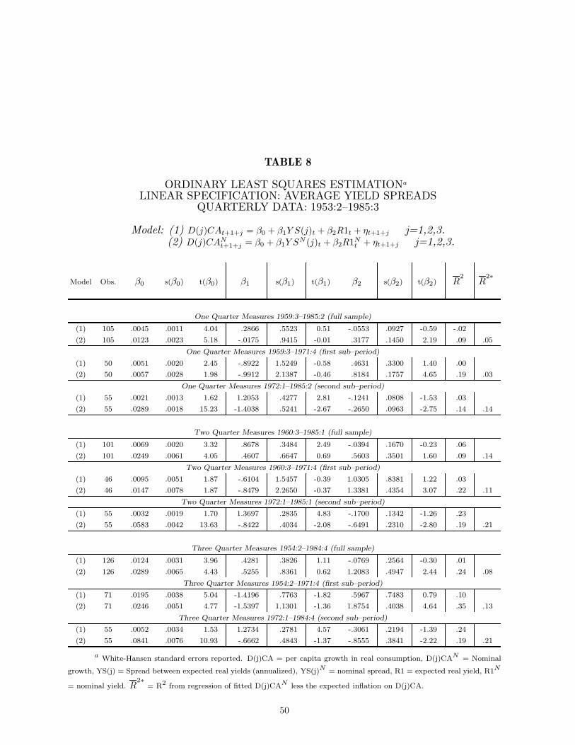
TABLE 8


LINEAR SPECIFICATION: AVERAGE YIELD SPREADSQUARTERLY DATA: 1953:2–1985:3

Model: (1) D(j)CAt+1+j = β0 + β1Y S(j)t + β2R1t + ηt+1+j j=1,2,3.(2) D(j)CAN

t+1+j = β0 + β1Y SN (j)t + β2R1Nt + ηt+1+j j=1,2,3.

Model Obs. β0 s(β0) t(β0) β1 s(β1) t(β1) β2 s(β2) t(β2) R2

R2∗

One Quarter Measures 1959:3–1985:2 (full sample)

(1) 105 .0045 .0011 4.04 .2866 .5523 0.51 -.0553 .0927 -0.59 -.02

(2) 105 .0123 .0023 5.18 -.0175 .9415 -0.01 .3177 .1450 2.19 .09 .05

One Quarter Measures 1959:3–1971:4 (first sub–period)

(1) 50 .0051 .0020 2.45 -.8922 1.5249 -0.58 .4631 .3300 1.40 .00

(2) 50 .0057 .0028 1.98 -.9912 2.1387 -0.46 .8184 .1757 4.65 .19 .03

One Quarter Measures 1972:1–1985:2 (second sub–period)

(1) 55 .0021 .0013 1.62 1.2053 .4277 2.81 -.1241 .0808 -1.53 .03

(2) 55 .0289 .0018 15.23 -1.4038 .5241 -2.67 -.2650 .0963 -2.75 .14 .14

Two Quarter Measures 1960:3–1985:1 (full sample)

(1) 101 .0069 .0020 3.32 .8678 .3484 2.49 -.0394 .1670 -0.23 .06

(2) 101 .0249 .0061 4.05 .4607 .6647 0.69 .5603 .3501 1.60 .09 .14

Two Quarter Measures 1960:3–1971:4 (first sub–period)

(1) 46 .0095 .0051 1.87 -.6104 1.5457 -0.39 1.0305 .8381 1.22 .03

(2) 46 .0147 .0078 1.87 -.8479 2.2650 -0.37 1.3381 .4354 3.07 .22 .11

Two Quarter Measures 1972:1–1985:1 (second sub–period)

(1) 55 .0032 .0019 1.70 1.3697 .2835 4.83 -.1700 .1342 -1.26 .23

(2) 55 .0583 .0042 13.63 -.8422 .4034 -2.08 -.6491 .2310 -2.80 .19 .21

Three Quarter Measures 1954:2–1984:4 (full sample)

(1) 126 .0124 .0031 3.96 .4281 .3826 1.11 -.0769 .2564 -0.30 .01

(2) 126 .0289 .0065 4.43 .5255 .8361 0.62 1.2083 .4947 2.44 .24 .08

Three Quarter Measures 1954:2–1971:4 (first sub–period)

(1) 71 .0195 .0038 5.04 -1.4196 .7763 -1.82 .5967 .7483 0.79 .10

(2) 71 .0246 .0051 4.77 -1.5397 1.1301 -1.36 1.8754 .4038 4.64 .35 .13

Three Quarter Measures 1972:1–1984:4 (second sub–period)

(1) 55 .0052 .0034 1.53 1.2734 .2781 4.57 -.3061 .2194 -1.39 .24

(2) 55 .0841 .0076 10.93 -.6662 .4843 -1.37 -.8555 .3841 -2.22 .19 .21

a White-Hansen standard errors reported. D(j)CA = per capita growth in real consumption, D(j)CAN = Nominal

growth, YS(j) = Spread between expected real yields (annualized), YS(j)N = nominal spread, R1 = expected real yield, R1N

= nominal yield. R2∗

= R2 from regression of fitted D(j)CAN less the expected inflation on D(j)CA.

50

TABLE 9


LINEAR SPECIFICATION: AVERAGE REAL YIELD SPREADSQUARTERLY DATA: 1953:2–1985:3

Model: D(j)CAt+j+1 = β0 + β1Y S(j)t + β2R(1)t + εt+j+1 j=1,2,3.

Obs. β0 s(β0) t(β0) β1 s(β1) t(β1) β2 s(β2) t(β2) χ2 d.f. Prob.


105 .0047 .0011 4.12 .1109 .7287 0.15 .0433 .1356 0.31 1.03 1 .69


101 .0078 .0028 2.76 .7644 .6664 1.14 -.0484 .2558 -0.18 2.09 1 .85


126 .0133 .0034 3.88 .2145 .7471 0.28 .3022 .5048 0.59 0.92 1 .66

aInstrumental estimation uses the technique of Hansen (1982). The standard errors are corrected for moving averagesinduced by the overlapping dependent variable and for conditional heteroskedasticity. The instrumentation consists of a constant,the expected real rate (parameters re-estimated at every point in the time series), the expected yield spread based on the timeseries model of inflation (parameters updated at every point in thetime series) and the logarithm of ratio of yields on Moody’sBBA and AAA rate bonds.

51

TABLE 10


LINEAR SPECIFICATION: AVERAGE INTEREST RATESANNUAL DATA: 1900–1984

Model: (1) D(1)CAt+1 = β0 + β1R(1)t + εt+1

(2) D(1)CANt+1 = β0 + β1R(1)N

t + εt+1


R2∗


(1) 84 .0186 .0029 6.44 -.1585 .1301 -1.22 .068

(2) 84 .0394 .01451 2.71 .1675 .2296 0.72 -.005 .064

first sub-period 1935–1984

(1) 50 .0207 .0032 6.45 .0655 .0815 0.80 -.004

(2) 50 .0542 .0122 4.41 .2084 .1770 1.17 .023 .073


(1) 31 .0182 .0033 5.38 .0740 .1082 0.68 -.020

(1)∗ 31 .0197 .0032 6.04 .0100 .0998 0.10 -.034

(2) 31 .0353 .0115 3.05 .4673 .1927 2.42 .273 .098

(2)∗ 31 .0337 .0102 3.28 .5097 .1881 2.70 .340 .059

a Standard errors corrected for moving average process in residuals and for conditional heteroskedasticity. SeeWhite (1980) and Hansen (1982). D(1)CA = Real per capita growth in Consumption of Non-Durables and Services,

D(1)CAN = Nominal Consumption growth, R(1) = expected real rate calculated by subtracting IMA(1,1) forecastson the inflation rate from the nominal interest rate on a corporate bond (parameters updated at every point in series),

R(1)N = Nominal interest rate, (Gov.) represents the nominal interest rate on a one year government bond. R2∗

=the coefficient of determination that results from the regression of the nominal consumption growth predictions less

the expected inflation rate on real consumption growth. (1)∗, (2)∗ calculated with yields on government instruments.

54

TABLE 11


LINEAR SPECIFICATION: AVERAGE REAL INTEREST RATESANNUAL DATA: 1900–1984

Model: D(1)CAt+1 = β0 + β1R(1)t + εt+1

Obs. β0 s(β0) t(β0) β1 s(β1) t(β1) χ2 d.f. Prob.


83 .0180 .0029 6.18 -.2158 .1255 -1.71 .0442 1 .16


50 .0208 .0033 6.32 .1346 .1036 1.30 5.2554 1 .97

aInstrumental estimation uses the technique of Hansen (1982). The standard errors are corrected for movingaverages induced by the overlapping dependent variable and for conditional heteroskedasticity. The dependent variableis the growth in real per capita consumption of non-durables and services. The regressor is the realized real rate ofinterest on a one year corporate bond. The instrumentation consists of a constant, the expected real rate (parametersre-estimated at every point in the time series), and the logarithm of ratio of yields on corporate 30 year and 1 yearbonds.

55

TABLE 12


LINEAR SPECIFICATION: AVERAGE YIELD SPREADSANNUAL DATA: 1900–1984

Model: (1) D(1)CAt+1 = β0 + β1Y S(1)t + β2R(1)t + ηt+1

(2) D(1)CANt+1 = β0 + β1Y S(1)N

t + β2R(1)Nt + ηt+1


R2∗


(1) 84 .0184 .0027 6.76 .0577 .2287 0.25 -.1627 .1246 -1.30 .06

(2) 84 .0421 .0138 3.03 -1.2019 .9552 -1.25 .2472 .2534 0.97 .03 .06


(1) 50 .0165 .0028 5.83 .6515 .2060 3.16 .0357 .0833 0.42 .04

(2) 50 .0564 .0124 4.53 -.4629 .4976 -0.93 .2316 .1745 1.32 .01 .05


(1) 31 .0174 .0032 5.32 .5231 .2566 2.03 -.0460 .1232 -0.37 .03

(1)* 31 .0149 .0049 3.03 1.4032 .9206 1.52 -.6434 .0947 -0.67 .02

(2) 31 .0373 .0099 3.75 -.8027 .5084 -1.57 .5282 .1736 3.04 .31 .02

(2)* 31 .0299 .0115 2.59 1.0637 1.7911 0.59 .4898 .1838 2.66 .33 .09

a Standard errors corrected for moving average process in residuals and for conditional heteroskedasticity. See White (1980)and Hansen (1982). D(1)CA = Real per capita growth in Consumption of Non-Durables and Services, R1 = real rate calculated

by subtracting IMA(1,1) forecasts on the inflation rate from the nominal corporate bond rate, D(1)CAN = nominal consumptiongrowth, R1 (Gov.) = real rate calculated by subtracting IMA(1,1) forecasts on the inflation rate from a one year nominal governmentbond rate. YS(1) = spread calculated as the difference between two expected real rates (annualized) on instruments with differenttime to maturity. Long term instrument is the yield on a one year corporate bond. Short term instrument is the yield on 90 day

commercial paper, 1900–1919, and 90 day Treasury bills, 1920-1984. YS(1)N = nominal yield spread, (1)*, (2)* = government bondis used as longer term instrument.

56

TABLE 13


LINEAR SPECIFICATION: AVERAGE REAL YIELD SPREADSANNUAL DATA: 1900–1984

Model: D(1)CAt+1 = β0 + β1Y S(1)t + β2R(1)t + εt+1

Obs. β0 s(β0) t(β0) β1 s(β1) t(β1) β2 s(β2) t(β2) χ2 d.f. Prob.


83 .0178 .0029 6.09 .2174 .4008 0.54 -.1677 .1112 -1.50 0.80 2 .33


51 .0143 .0054 2.65 1.0079 .6295 1.60 .0304 .1170 0.26 4.05 2 .87

aInstrumental estimation uses the technique of Hansen (1982). The standard errors are corrected for moving averagesinduced by the overlapping dependent variable and for conditional heteroskedasticity. The instrumentation consists of a constant,the expected real rate on a short term bill and a one year corporate bond (parameters re-estimated at every point in the timeseries), the lagged yield spread and the logarithm of ratio of yields on 30 year to 1 year corporate bonds.

57

TABLE 14


NON-LINEAR SPECIFICATION: AVERAGE REAL INTEREST RATESQUARTERLY DATA: 1953:4–1985:3

Model: (1) Et[δj{ Ct

Ct+j}α(1 + R1,t+j) − 1] = 0 j = 1, 2, 3, 4.

(2) Et[δjeα(Ct−Ct+j)(1 + R1,t+j) − 1] = 0 j = 1, 2, 3, 4.

Model Obs. α s(α) t(α) δ s(δ) t(δ) χ2 d.f. Prob.


(1) 128 .6467 .5497 1.17 1.0019 .0025 393.67 6.87 2 .97

(2) 128 .0267 .0901 0.29 .9993 .0029 344.75 9.68 2 .99


(1) 105 1.1167 1.8889 0.59 1.0027 .0093 108.09 2.21 2 .67

(2) 105 .0310 .1762 0.17 .9985 .0062 161.07 7.21 2 .97


(1) 101 .7910 2.0797 0.38 1.0006 .0118 84.96 1.81 2 .59

(2) 101 .0717 .1434 0.50 0.9993 .0053 188.36 6.02 2 .95


(1) 126 1.3417 1.9042 0.70 1.0025 .0094 106.00 2.52 2 .72

(2) 126 .0705 .5961 0.11 .9978 .0038 256.11 3.79 2 .85

aInstrumental estimation uses the technique of Hansen (1982). The standard errors are corrected for amoving averages process in the errors for conditional heteroskedasticity. Ct/Ct+1 is the ratio of real per capitaconsumption of non-durables and services, R1,t+1 is the realized real rate of interest on a one year corporate bond.

The instrumentation consists of a constant, the expected real j–period rate (parameters re-estimated at every pointin the time series), lagged consumption ratio or difference and the difference in yields on Moody’s AAA and BAArated bonds.

64

TABLE 15


NON-LINEAR SPECIFICATION: AVERAGE REAL INTEREST RATESANNUAL DATA: 1900–1984

Model: (1) Et[δ{ Ct

Ct+1}α(1 + R1,t+1) − 1] = 0

(2) Et[δeα(Ct−Ct+1)(1 + R1,t+1) − 1] = 0

Model Obs. α s(α) t(α) δ s(δ) t(δ) χ2 d.f. Prob.


(1) 83 -5.3008 4.3383 -1.22 .9046 .0728 12.42 0.02 1 .12

(2) 83 -3.2122 5.4271 -0.59 .8863 .1835 4.83 0.06 1 .19


(1) 51 1.6637 1.8805 0.88 1.0314 .0459 22.44 1.81 1 .82

(2) 51 .9001 .4882 1.84 1.0468 .0297 35.24 2.72 1 .90


(1) 32 1.8420 1.3754 1.33 1.0271 .0311 33.03 1.22 1 .73

(2) 32 .6973 .3508 1.98 1.0255 .0228 45.01 1.32 1 .75

aInstrumental estimation uses the technique of Hansen (1982). The standard errors are corrected for amoving averages process in the errors for conditional heteroskedasticity. Ct/Ct+1 is the ratio of real per capitaconsumption of non-durables and services. R1,t+1 is the realized real rate of interest on a one year corporate bond.

The instrumentation consists of a constant, the expected real 1 year rate and the expected short term real rate(parameters re-estimated at every point in the time series).

66

TABLE 16

ALTERNATIVE PREDICTORS OF CONSUMPTION GROWTH:LAGGED CONSUMPTION AND REAL STOCK RETURNS

QUARTERLY DATA: 1953:2–1985:3

Model (1): D(j)CAt+j = β0 + β1D(1)CAt + εt+j j=1,2,3,4.(2): D(j)CAt+j = β0 + β1R(j)V Wt + εt+j j=1,2,3,4.



(1) 130 .0035 .0006 6.00 .2464 .0738 3.33 .05

(2) 130 .0043 .0006 7.81 .0198 .0052 3.82 .08


(1) 105 .0078 .0013 5.90 .3864 .1411 2.73 .05

(2) 105 .0094 .0013 7.05 .0124 .0067 1.83 .02


(1) 101 .0114 .0023 5.06 .6648 .1278 5.20 .10

(2) 101 .0141 .0021 6.69 .0201 .0079 2.52 .06


(1) 126 .0156 .0022 7.00 .5941 .0956 6.21 .06

(2) 126 .0172 .0022 7.72 .0210 .0071 2.95 .07

Standard errors corrected for moving average process in residuals and for conditional heteroskedasticity. SeeWhite (1980) and Hansen (1982). D(j)CA = Real per capita j-period growth in Consumption of Non-Durables andServices. R(j)VW = Real j–period returns on the Value Weighted NYSE index.

70

TABLE 16



Model (1): D(j)CAt+j = β0 + β1D(1)CAt + εt+j j=1,2,3,4.(2): D(j)CAt+j = β0 + β1R(j)V Wt + εt+j j=1,2,3,4.



(1) 130 .0035 .0006 6.00 .2464 .0738 3.33 .05

(2) 130 .0043 .0006 7.81 .0198 .0052 3.82 .08


(1) 105 .0078 .0013 5.90 .3864 .1411 2.73 .05

(2) 105 .0094 .0013 7.05 .0124 .0067 1.83 .02


(1) 101 .0114 .0023 5.06 .6648 .1278 5.20 .10

(2) 101 .0141 .0021 6.69 .0201 .0079 2.52 .06


(1) 126 .0156 .0022 7.00 .5941 .0956 6.21 .06

(2) 126 .0172 .0022 7.72 .0210 .0071 2.95 .07

Standard errors corrected for moving average process in residuals and for conditional heteroskedasticity. SeeWhite (1980) and Hansen (1982). D(j)CA = Real per capita j-period growth in Consumption of Non-Durables andServices. R(j)VW = Real j–period returns on the Value Weighted NYSE index.

70

TABLE 17



Model (1): D(j)CAt+1+j = β0 + β1D(1)CAt + εt+1+j j=1,2,3.(2): D(j)CAt+1+j = β0 + β1R(j)V Wt + εt+1+j j=1,2,3.



(1) 105 .0041 .0007 5.80 .1532 .0797 1.92 .01

(2) 105 .0048 .0006 7.56 .0029 .0049 0.59 -.01


(1) 50 .0041 .0009 4.29 .2633 .0963 2.73 .05

(2) 50 .0056 .0008 7.13 -.0022 .0076 -0.29 -.02


(1) 55 .0039 .0010 3.91 .0497 .1199 0.41 -.02

(2) 55 .0041 .0009 4.35 .0057 .0061 0.92 -.01


(1) 101 .0077 .0014 5.35 .4297 .0756 5.68 .07

(2) 101 .0095 .0014 6.99 .0125 .0068 1.82 .02


(1) 46 .0097 .0019 5.02 .3106 .0897 3.46 .02

(2) 46 .0115 .0017 6.59 .0032 .0077 0.41 -.02


(1) 55 .0065 .0019 3.41 .4413 .0074 5.92 .06

(2) 55 .0081 .0019 4.23 .0168 .0090 1.86 .04


(1) 126 .0124 .0021 5.77 .4231 .1317 3.21 .04

(2) 126 .0136 .0019 7.27 .0154 .0063 2.46 .04


(1) 71 .0144 .0024 5.88 .2770 .1605 1.72 .01

(2) 71 .0146 .0020 7.44 .0216 .0078 2.76 .08


(1) 55 .0102 .0033 3.08 .5340 .0877 6.09 .05

(2) 55 .0122 .0033 3.70 .0082 .0082 1.00 -.00

Standard errors corrected for moving average process in residuals and for conditional heteroskedasticity. SeeWhite (1980) and Hansen (1982). D(j)CA = Real per capita j–period growth in Consumption of Non-Durables andServices. R(j)VW = Real j–period returns on the Value Weighted NYSE index.

71

TABLE 18

COMPARISON OF FORECASTS:INTEREST RATE MODEL VS. ALTERNATIVE MODELS


Model (1): D(j)CAt+j = β0 + β1(Real Y ield F itted)t + β2(Cons. AR Fitted)t + εt+j

(2): D(j)CAt+j = β0 + β1(Real Y ield F itted)t + β2(Stocks F itted)t + εt+j

(3): D(j)CAt+j = β0 + β1(Nominal Y ield F itted)t + β2(Cons. AR Fitted)t + εt+j

(4): D(j)CAt+j = β0 + β1(Nominal Y ield F itted)t + β2(Stocks F itted)t + εt+j



(1) 130 -.0079 .0052 -1.52 1.6666 1.1209 1.48 1.0605 .3044 3.48 .06

(2) 130 -.0048 .0050 -0.95 1.0460 1.1452 0.91 1.0019 .2646 3.78 .08

(3) 130 .0001 .0014 0.04 .0859 .0887 0.96 .8977 .2997 2.99 .05

(4) 130 -.0002 .0014 -0.15 .1081 .0941 1.14 .9385 .2507 3.74 .08


(1) 105 -.0135 .0116 -1.16 1.3523 1.1701 1.15 1.0413 .3671 2.83 .05

(2) 105 -.0117 .0123 -0.94 1.1795 1.3455 0.87 1.0329 .5661 1.82 .02

(3) 105 .0019 .0034 0.55 .1853 .0832 2.22 .6172 .3741 1.64 .10

(4) 105 .0016 .0045 0.36 .2067 .0920 2.24 .6184 .4316 1.43 .09


(1) 101 .0320 .1281 0.24 -2.1961 8.6824 -0.25 1.0103 .1858 5.43 .09

(2) 101 .0279 .1382 0.20 -1.9138 9.2674 -0.20 1.0116 .3773 2.68 .05

(3) 101 .0026 .0024 1.10 .2165 .0975 2.22 .5982 .1341 4.46 .18

(4) 101 .0024 .0060 0.40 .2331 .1086 2.14 .5947 .3909 1.52 .18


(1) 126 .1413 .3621 0.38 -7.7082 19.6334 -0.39 1.0279 .1333 7.71 .05

(2) 126 .1362 .3387 0.40 -7.4328 18.3178 -0.40 1.0207 .3268 3.12 .07

(3) 126 .0027 .0007 3.79 .1355 .0998 1.35 .7123 .1463 4.86 .09

(4) 126 .0026 .0055 0.47 .1220 .1149 1.06 .7312 .3635 2.01 .10

Standard errors corrected for moving average process in residuals and for conditional heteroskedasticity. SeeWhite (1980) and Hansen (1982). D(j)CA = Real per capita growth in Consumption of Non-Durables and Services(j=1,2,3,4).

72

TABLE 19COMPARISON OF FORECASTS:

YIELD SPREAD MODEL VS. ALTERNATIVE MODELSQUARTERLY DATA: 1953:2–1985:3

Model (1): D(j)CAt+1+j = β0 + β1(Real Spread F itted)t + β2(Cons. AR Fitted)t + εt+1+j

(2): D(j)CAt+1+j = β0 + β1(Real Spread F itted)t + β2(Stocks F itted)t + εt+1+j

(3): D(j)CAt+1+j = β0 + β1(Nominal Spread F itted)t + β2(Cons. AR Fitted)t + εt+1+j

(4): D(j)CAt+1+j = β0 + β1(Nominal Spread F itted)t + β2(Stocks F itted)t + εt+1+j



(1) 105 -.0059 .0071 -0.83 1.1882 1.3387 0.88 1.0456 .5150 2.03 .01

(2) 105 -.0055 .0110 -0.49 1.0426 1.4585 0.71 1.0976 1.7262 0.63 -.01

(3) 105 .0015 .0027 0.56 .1954 .1061 1.84 .4804 .5971 0.80 .04

(4) 105 .0029 .0075 0.38 .2207 .0995 2.21 .1737 1.5514 0.11 .04


(1) 50 -.0022 .0040 -0.54 .5846 .7717 0.75 .8103 .4005 2.02 .04

(2) 50 -.0054 .0200 -0.26 .9990 .7003 1.42 .9652 3.4264 0.28 .00

(3) 50 -.0110 .0026 -0.42 .3629 .3842 0.94 .8064 .4254 1.89 .04

(4) 50 -.0043 .0194 -0.22 .5704 .3512 1.62 1.1601 3.3808 0.34 .01


(1) 55 -.0011 .0092 -0.12 .9920 .3521 2.81 .2874 2.3116 0.12 .03

(2) 55 -.0046 .0041 -1.12 1.0155 .3438 2.95 1.1141 1.0746 1.03 .04

(3) 55 .0280 .0107 2.61 .4998 .1064 4.69 -6.3168 2.6367 -2.39 .19

(4) 55 .0034 .0040 0.85 .3377 .1036 3.25 -.1717 .9595 -0.17 .12


(1) 101 -.0071 .0036 -1.98 .8691 .3702 2.34 .8630 .1672 5.16 .12

(2) 101 -.0067 .0049 -1.34 .9152 .4179 2.18 .7729 .5064 1.52 .08

(3) 101 .0023 .0019 1.18 .2336 .0957 2.44 .5292 .1877 2.81 .15

(4) 101 .0027 .0070 0.39 .2607 .0933 2.79 .4510 .6865 0.65 .14


(1) 46 -.0044 .0060 -0.73 .8200 .7984 1.02 .5622 .4892 1.14 .04

(2) 46 -.0212 .0280 -0.76 1.0448 .6924 1.50 1.7915 2.2580 0.79 .04

(3) 46 -.0022 .0048 -0.47 .6589 .3872 1.70 .4744 .4848 0.97 .10

(4) 46 -.0051 .0050 -1.01 .6830 .3769 1.81 .7039 .4985 1.41 .11


(1) 46 -.0024 .0013 -1.83 .9293 .2192 4.23 .3566 .1534 2.32 .24

(2) 55 -.0036 .0032 -1.10 .9364 .2198 4.26 .4978 .3278 1.51 .25

(3) 55 .0062 .0032 1.95 .3408 .1266 2.69 -.0763 .3531 -0.21 .20

(4) 55 .0067 .0109 0.61 .3362 .1104 3.04 -.1285 1.2711 -0.10 .19


(1) 126 -.0115 .0127 -0.90 .8645 .8439 1.02 .9408 .3133 3.00 .05

(2) 126 -.0151 .0126 -1.20 1.0390 .8552 1.21 1.0185 .4103 2.48 .06

(3) 126 .0035 .0043 0.82 .1760 .1170 1.50 .5721 .3184 1.79 .09

(4) 126 .0036 .0064 0.55 .1734 .1243 1.39 .5725 .4759 1.20 .09


(1) 71 -.0037 .0088 -0.42 .9625 .5011 1.92 .2726 .5061 0.53 .10

(2) 71 -.0147 .0085 -1.72 .9711 .4391 2.21 .9596 .3278 2.92 .18

(3) 71 .0104 .0109 0.95 .5443 .2529 2.15 -.2403 .7690 -0.31 .12

(4) 71 -.0017 .0055 -0.30 .4308 .2346 1.83 .6439 .3592 1.79 .15


(1) 55 -.0033 .0032 -1.01 .9421 .2497 3.77 .3243 .2599 1.24 .24

(2) 55 -.0107 .0123 -0.86 .9941 .1991 4.99 .8722 .9753 0.89 .25

(3) 55 .0106 .0060 1.77 .2884 .1321 2.18 -.1379 .4925 -0.28 .19

(4) 55 .0168 .0172 0.98 .2936 .1206 2.43 -.6489 1.3765 -0.47 .20

Standard errors corrected for moving average process in residuals and for conditional heteroskedasticity. SeeWhite (1980) and Hansen (1982). Real per capita growth in Consumption of Non-Durables and Services, (j=1,2,3).

73

TABLE 20


ANNUAL DATA: 1900–1984

Model (1): D(1)CAt+1 = β0 + β1D(1)CAt + εt+1

(2): D(1)CAt+1 = β0 + β1R(1)V Wt + εt+1



(1) 84 .0081 .0036 2.25 .4980 .1247 3.99 .24

(2) 84 .0148 .0042 3.53 .0251 .0281 0.89 .02


(1) 50 .0165 .0022 7.54 .2168 .0860 2.51 .03

(2) 50 .0199 .0029 6.86 .0203 .0094 2.14 .01


(1) 31 .0150 .0022 6.93 .2553 .0996 2.56 .03

(2) 31 .0187 .0026 7.17 .0212 .0085 2.49 .02

Standard errors corrected for moving average process in residuals and for conditional heteroskedasticity. SeeWhite (1980) and Hansen (1982). D(1)CA = Real per capita growth in Consumption of Non-Durables and Services,R(1)VW = Real j–period returns on the Standard and Poors stock index, 1926–1984, and the Cowles Commissionindex, 1900–1925.

75

TABLE 21

COMPARISON OF FORECASTS:INTEREST RATE MODEL VS. ALTERNATIVE MODELS


Model (1): D(1)CAt+1 = β0 + β1(Real Y ield F itted)t + β2(Cons. AR Fitted)t + εt+1

(2): D(1)CAt+1 = β0 + β1(Real Y ield F itted)t + β2(Stocks F itted)t + εt+1

(3): D(1)CAt+1 = β0 + β1(Nominal Y ield F itted)t + β2(Cons. AR Fitted)t + εt+1

(4): D(1)CAt+1 = β0 + β1(Nominal Y ield F itted)t + β2(Stocks F itted)t + εt+1



(1) 84 -.5782 .0101 -0.56 .4427 .4394 1.00 .9139 .1836 4.97 .25

(2) 84 -.0155 .0222 -0.69 .9881 .7351 1.34 .9682 .8219 1.17 .09

(3) 84 .0030 .0031 0.96 -.0794 .0794 -1.00 .9176 .1774 5.17 .25

(4) 84 .0025 .0127 0.19 -.1772 .1328 -1.33 1.0767 .8063 1.33 .09


(1) 50 -.0296 .0171 -1.73 1.2887 1.0252 1.25 1.1164 .3525 3.16 .03

(2) 50 -.0167 .0280 -0.59 .8673 1.1939 0.72 .9253 .4621 2.00 -.00

(3) 50 -.0050 .0062 -0.80 .2035 .0772 2.63 .9692 .4152 2.33 .10

(4) 50 .0058 .0087 0.66 .1902 .0833 2.28 .4716 .4032 1.16 .06


(1) 31 -.0297 .0227 -1.34 1.3874 1.0132 1.36 1.0993 .4664 2.35 .02

(2) 31 -.0134 .0230 -0.58 .7259 1.2084 0.60 .9444 .4324 2.18 -.01

(3) 31 -.0056 .0118 -0.47 .2955 .1449 2.03 .8750 .5297 1.65 .12

(4) 31 .0087 .0117 0.74 .2968 .1908 1.55 .1580 .7508 0.21 .07

(1)a 31 -.0211 .1491 -0.14 1.0582 7.5020 0.14 1.0002 .3977 2.51 -.00

(2)a 31 .0236 .1700 0.13 -1.1950 8.4963 -0.14 1.0108 .3897 2.59 -.02

(3)a 31 -.0029 .0102 -0.28 .2526 .1683 1.50 .7990 .5381 1.48 .07

(4)a 31 .0062 .0090 0.68 .2486 .2236 1.11 .3472 .6548 0.53 .03

Standard errors corrected for moving average process in residuals and for conditional heteroskedasticity. See

White (1980) and Hansen (1982). a Estimated with government one year bond.

76

TABLE 22

COMPARISON OF FORECASTS:YIELD SPREAD MODEL VS. ALTERNATIVE MODELS


Model (1): D(1)CAt+1 = β0 + β1(Real Y ield F itted)t + β2(Cons. AR Fitted)t + εt+1

(2): D(1)CAt+1 = β0 + β1(Real Y ield F itted)t + β2(Stocks F itted)t + εt+1

(3): D(1)CAt+1 = β0 + β1(Nominal Y ield F itted)t + β2(Cons. AR Fitted)t + εt+1

(4): D(1)CAt+1 = β0 + β1(Nominal Y ield F itted)t + β2(Stocks F itted)t + εt+1



(1) 84 -.0063 .0102 -0.62 .4790 .4404 1.08 .9121 .1872 4.87 .25

(2) 84 -.0155 .0222 -0.69 .9877 .7269 1.35 .9670 .8280 1.16 .09

(3) 84 .0034 .0035 0.94 -.1033 .0780 -1.32 .9259 .1961 4.72 .26

(4) 84 .0027 .0136 0.19 -.1769 .1309 -1.35 1.0645 .8555 1.24 .08


(1) 50 -.0332 .0105 -3.16 1.2259 .3055 4.01 1.3502 .4627 2.91 .13

(2) 50 -.0190 .0126 -1.50 .9760 .3275 2.98 .9258 .5455 1.69 .07

(3) 50 -.0039 .0058 -0.66 .1764 .0796 2.21 .9516 .4181 2.27 .08

(4) 50 .0048 .0084 0.56 .1629 .0846 1.92 .5577 .3959 1.40 .04


(1) 31 -.0415 .0163 -2.55 1.4673 .4231 3.46 1.6132 .4682 3.44 .19

(2) 31 -.0205 .0196 -1.04 1.0090 .2384 4.23 1.0168 .5291 1.92 .09

(3) 31 -.0014 .0087 -0.16 .1785 .1960 0.91 .8262 .5397 1.53 .03

(4) 31 .0037 .0069 0.53 .1517 .2661 0.57 .6080 .6450 0.94 -.00

(1)a 31 -.0137 .0096 -1.42 .8679 .5760 1.50 .8191 .5062 1.61 .06

(2)a 31 -.0211 .0144 -1.46 1.0221 .6337 1.61 1.0365 .4320 2.39 .08

(3)a 31 -.0021 .0104 -0.20 .2711 .1451 1.86 .7328 .5501 1.33 .09

(4)a 31 .0076 .0101 0.75 .2835 .1866 1.51 .2311 .6420 0.35 .06

Standard errors corrected for moving average process in residuals and for conditional heteroskedasticity. See

White (1980) and Hansen (1982). a Estimated with government one year bond.

77

TABLE 23

EVALUATION OF OUT-OF-SAMPLE FORECASTING PERFORMANCE:CONSUMPTION GROWTH FORECASTING MODELS

Model Horizon Forecasts RMSE MAE

Yield Spread (Real) 1 Quarter 37 0.005228 0.004185Lagged Consumption 1 Quarter 37 0.005186 0.004008

Value Weighted Stocks 1 Quarter 37 0.005172 0.004021Yield Spread (Nominal) 1 Quarter 37 0.006297 0.005262





Yield Spread (Real) 1 Year 9 0.017123 0.013389Lagged Consumption 1 Year 9 0.014930 0.011409

Value Weighted Stocks 1 Year 9 0.015837 0.012796Yield Spread (Nominal) 1 Year 9 0.020500 0.018807

Parameters of each model are re–estimated at each point in the time series during 1975:4–1984:4. These parameters are used to forecast the 1976:1–1985:1 period for the quarterly modelsand 1976–1984 for the annual model.

79

TABLE 24

COMPARISON OF OUT-OF-SAMPLE FORECASTING PERFORMANCEWITH THE COMMERCIAL MACROECONOMIC FORECASTING SERVICES

Model Spana Variable Forecasts RMSE MAE

Yield Spread 1 Total Consumption (Nominal) 37 3.1 2.5Data Resources 1 Total Consumption (Nominal) 37 3.4 2.7

Chase Econ. 1 Total Consumption (Nominal) 37 3.3 2.7Yield Spread 2 Total Consumption (Nominal) 37 2.3 1.9

Data Resources 2 Total Consumption (Nominal) 37 2.6 2.2Chase Econ. 2 Total Consumption (Nominal) 37 2.7 2.1Yield Spread 3 Total Consumption (Nominal) 37 1.9 1.7

Data Resources 3 Total Consumption (Nominal) 37 2.1 1.7Chase Econ. 3 Total Consumption (Nominal) 37 2.5 1.9Yield Spread 1 Gross National Product (Real) 37 4.7 3.7

Data Resources 1 Gross National Product (Real) 37 3.8 3.1Chase Econ. 1 Gross National Product (Real) 37 4.0 3.3Yield Spread 2 Gross National Product (Real) 37 3.6 2.8

Data Resources 2 Gross National Product (Real) 37 2.8 2.2Chase Econ. 2 Gross National Product (Real) 37 3.1 2.5Yield Spread 3 Gross National Product (Real) 37 3.3 2.8

Data Resources 3 Gross National Product (Real) 37 2.4 1.9Chase Econ. 3 Gross National Product (Real) 37 2.7 2.3Yield Spread 1 Non. Res. Fixed Inv. (Real) 37 13.1 10.2

Data Resources 1 Non. Res. Fixed Inv. (Real) 37 10.2 8.2Chase Econ. 1 Non. Res. Fixed Inv. (Real) 37 10.8 8.2Yield Spread 2 Non. Res. Fixed Inv. (Real) 37 11.4 9.1

Data Resources 2 Non. Res. Fixed Inv. (Real) 37 8.9 7.3Chase Econ. 2 Non. Res. Fixed Inv. (Real) 37 9.8 7.9Yield Spread 3 Non. Res. Fixed Inv. (Real) 37 10.4 8.4

Data Resources 3 Non. Res. Fixed Inv. (Real) 37 8.3 6.6Chase Econ. 3 Non. Res. Fixed Inv. (Real) 37 9.7 7.9Yield Spread 1 Housing Starts 37 44.5 38.5

Data Resources 1 Housing Starts 37 39.9 29.3Chase Econ. 1 Housing Starts 37 50.9 34.9Yield Spread 2 Housing Starts 37 34.4 28.3

Data Resources 2 Housing Starts 37 28.9 23.3Chase Econ. 2 Housing Starts 37 36.7 28.9Yield Spread 3 Housing Starts 37 30.4 24.9

Data Resources 3 Housing Starts 37 28.9 20.5Chase Econ. 3 Housing Starts 37 31.4 22.1

Parameters of each model are re–estimated at each point in the time series during 1975:4–1984:4. These parameters are used to forecast the 1976:1–1985:1 period. a “1” represents onequarter growth forecast.

85

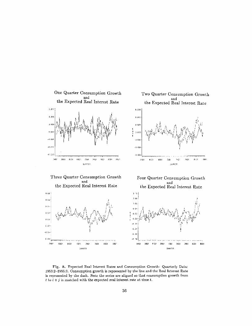
APPENDIX A

THE CONSUMER’S PLANNING PROBLEMA MORE DETAILED EXAMINATION

88

Consider a pure exchange economy with a representative agent with additivelyseparable utility receiving a stochastic endowment. This agent can choose toconsume this endowment or invest in a portfolio of j–period bonds, {Bj,t : j =1, . . . , k}. The bonds are assumed to be default free. Expectations at time t areconditioned on the information set Ft – which contains all the information aboutthe environment available at time t. Consumption Ct is required to be measurableat t with respect to Ft. The consumer maximizes the following objective:

max{Ct,Bj,t}∞

t=0 j=1,...,k

∞∑

t=0

δtE0U(Ct); 0 < δ < 1,

subject to:

CNt +

k∑

j=1

Bj,t ≤ Y Nt +

k∑

j=1

Bj,t−j(1 + RNj,t−j), (A.1)

where Ct is the agent’s real consumption, CNt represents nominal consumption,

RNj,t−j is the nominal yield on a j–period bond bought at time t− j, Et is the ex-

pectation operator conditioned on information Ft, Y Nt is the nominal endowment1

and δ is the consumer’s constant time discount factor. Form the Lagrangian L:

L = E0

∞∑

t=0

δt

U(Ct) + λt(YtPt +

k∑

j=1

Bj,t−j(1 + Rj,t−j) − CtPt −k∑

j=1

Bj,t)

(A.2)

The first-order conditions are:

1 The conditional expectation Et[Y Nt+j ] is assumed to exist for all j ≥ 1.

89

Ct : U ′(Ct) − Ptλt = 0

Bj,t : −λt + δjEtλt+j(1 + RNj,t) = 0 j = 1, . . . , k.

Solve the first condition for λt and substitute this into the second:

U ′(Ct)Pt

= δjEtU ′(Ct+j)

Pt+j(1 + RN

j,t)

1 = δjEtU ′(Ct+j)U ′(Ct)

Pt

Pt+j(1 + RN

j,t)

Substitute the real interest rate, Rj,t times the inflation rate on the RHS and theEuler equation (2.2) of chapter 2 obtains:

E

[δj U ′(Ct+j)

U ′(Ct)(1 + Rj,t) − 1

∣∣∣∣ Ft

]= 0, for j = 1, . . . , k, (A.3)

The consumer’s problem does not restrict the agent from selling the bonds beforematurity. Bj,t can be positive or negative. Other assets can also enter into theproblem. They will not affect the basic first-order conditions. Note that to keepthe consumer’s problem well behaved, the arbitrary rolling over of debt is ruledout. Essentially, a limitation on the terminal value of the debt is imposed.

90

APPENDIX B

THE GMM WEIGHTING MATRIX

91

Let j be the order of the moving average process in the error. Hansen (1982)and Hansen and Singleton (1982) show that the weighting matrix for a first ordermoving average process (presented in Chapter 2 equation 2.14) is:

W ∗T =

[T∑

t=1

[h(xt+1, θT )Zt][h(xt+1, θT )Zt]′]−1

(B.1)

More generally, if j ≥ 0 then the matrix is formed by:

Rt(i) =1T

T∑

t=1+i

[h(xt+i, θT )Zt][h(xt+j−i, θT )Zt−i]′

W ∗T =

[RT (0) +

j−1∑

i=1

[Rt(i) + Rt(i)′]

]−1

(B.2)

Note that an estimate of the parameter vector θt is necessary before solving forthe weighting matrix. The standard estimation procedure proceeds in two stages.First, a sub-optimal choice of the weighting matrix, such as the identity matrix, ischosen and parameters are solved for. The initial parameter estimates are used tosolve for the optimal weighting matrix W ∗

T . This matrix is used in the objectivefunction and the final parameter vector θ∗t is solved for.

92

APPENDIX C

DATA SOURCES AND DEFINITIONS

93

Quarterly Data Set

Variable Description∗

NNIA Population used to calculate per-capita income. Millions ofpersons, middle of quarter, not seasonally adjusted.Source: U.S. Department of Commerce, Bureau of Economic

Analysis, National Income and Product Accounts ofthe United States, Table 2.1.

Span: 1946:1 to 1985:3

CDNS Personal consumption expenditures - durable goods. Billions ofdollars, not seasonally adjusted at quarterly rates.Source: U.S. Department of Commerce, Bureau of Economic


Span: 1946:1 to 1983:4Note: 1984:1 to 1985:3 data were not available at this time.

These four quarters were estimated by extrapolating thethe 1983 seasonal factors to 1984, dividing the 1984:1to 1985:3 seasonally adjusted data by these factorsto recover estimates of CDNS.

CNNS Personal consumption expenditures - non-durable goods. Billionsof dollars, not seasonally adjusted at quarterly rates.Source: U.S. Department of Commerce, Bureau of Economic



These four quarters were estimated by extrapolating thethe 1983 seasonal factors to 1984, dividing the 1984:1to 1985:3 seasonally adjusted data by these factorsto recover estimates of CNNS.

CSNS Personal consumption expenditures - service goods. Billionsof dollars, not seasonally adjusted at quarterly rates.Source: U.S. Department of Commerce, Bureau of Economic



94

These four quarters were estimated by extrapolating thethe 1983 seasonal factors to 1984, dividing the 1984:1to 1985:3 seasonally adjusted data by these factorsto recover estimates of CSNS.

PCD Implicit Price Deflator - Total Durables Index, 1982=1.0,seasonally adjusted at annual rates,Source: U.S. Department of Commerce, Bureau of Economic

Analysis, unpublished data from National Incomeand Product Accounts of the United States.

Span: 1946:1 to 1985:3

PCN Implicit Price Deflator - Total Non-Durables Index, 1982=1.0,seasonally adjusted at annual rates,Source: U.S. Department of Commerce, Bureau of Economic


Span: 1946:1 to 1985:3

PCS Implicit Price Deflator - Total Services Index, 1982=1.0,seasonally adjusted at annual rates,Source: U.S. Department of Commerce, Bureau of Economic


Span: 1946:1 to 1985:3

CDNS82 = CDNS/PCD

CNNS82 = CNNS/PCN

CSNS82 = CSNS/PCS

CANS82 = CNNS82 + CSNS82

CDNS82P = CDNS82/NNIA

CNNS82P = CNNS82/NNIA

CSNS82P = CSNS82/NNIA

CANS82P = CANS82/NNIA

D4CDt = log(CDNS82Pt) - log(CDNS82Pt−4)

D4CNt = log(CNNS82Pt) - log(CNNS82Pt−4)

D4CSt = log(CSNS82Pt) - log(CSNS82Pt−4)

D4CAt = log(CANS82Pt) - log(CANS82Pt−4)

CD82 Personal consumption expenditures - durable goods. Billionsof dollars, seasonally adjusted at annual rates.

95

Source: U.S. Department of Commerce, Bureau of EconomicAnalysis, unpublished data from the National Incomeand Product Accounts of the United States.

Span: 1946:1 to 1985:3

CN82 Personal consumption expenditures - non-durable goods. Billionsof dollars, seasonally adjusted at annual rates.Source: U.S. Department of Commerce, Bureau of Economic

Analysis, unpublished data from the National Incomeand Product Accounts of the United States.

Span: 1946:1 to 1985:3

CS82 Personal consumption expenditures - service goods. Billionsof dollars, seasonally adjusted at annual rates.Source: U.S. Department of Commerce, Bureau of Economic

Analysis, unpublished data from the National Incomeand Product Accounts of the United States.

Span: 1946:1 to 1985:3

CD82P = CD82/NNIA

CN82P = CN82/NNIA

CS82P = CS82/NNIA

CA82P = CN82P + CS82P

D1CDt = log(CD82Pt) - log(CD82Pt−1)

D1CNt = log(CN82Pt) - log(CN82Pt−1)

D1CSt = log(CS82Pt) - log(CS82Pt−1)

D1CAt = log(CA82Pt) - log(CA82Pt−1)

Y1 = Yield on 3 month U.S. Government Treasury Bills. Percent perannum, quoted on bank discount basis, not seasonally adjusted.Weekly averages computed from daily closing bid prices.Source: Federal Reserve Bulletin, Selected Interest Rates

and Bond Prices, and Data Resources Inc.,mneumonic=“RMGBS3NS”.

Note: Data available monthly. Converted to quarterly byarithmetic average.

Span: 1947:1 to 1985:4

Y2 = Yield on 6 month U.S. Government Treasury Bills. Percent perannum, quoted on bank discount basis, not seasonally adjusted.Weekly averages computed from daily closing bid prices.Source: Federal Reserve Bulletin, Selected Interest Rates

and Bond Prices, and Data Resources Inc.,mneumonic=“RMGBS6NS”.

96


Span: 1959:1 to 1985:4

Y3 = Yield on 9 to 12 month U.S. Government Treasury Bills. Percent perannum, quoted on bank discount basis, not seasonally adjusted.Weekly averages computed from daily closing bid prices.Source: Federal Reserve Bulletin, Selected Interest Rates

and Bond Prices, and Data Resources Inc.,mneumonic=“RMGBS9@12NS”.


Span: 1959:4 to 1985:4

Y4 = Yield on 1 year U.S. Government Treasury Bonds. Percent perannum, average of daily figures, not seasonally adjusted.Source: Federal Reserve Bulletin, Selected Interest Rates

and Bond Prices, and Data Resources Inc.,mneumonic=“RMGFCM@1NS”.

Note: Data available monthly. Converted to quarterly byarithmetic average.Span: 1953:2 to 1985:4




Span: 1976:3 to 1985:4




Span: 1953:2 to 1985:4

Y20 = Yield on 5 year U.S. Government Treasury Bond. Percent perannum, average of daily figures, not seasonally adjusted.Source: Federal Reserve Bulletin, Selected Interest Rates



Span: 1953:2 to 1985:4

97

Annual Data Set

Variable Description

POP Total population of the United States in millions. Before1930 excludes armed forces stationed overseas.Source: 1871-1970, U.S. Department of Commerce, Long-Term

Economic Growth 1860-1970,1971-1979, U.S. Department of Commerce, Bureau of theCensus, Current Population Reports,series P-251980-1984, U.S. Department of Commerce, Bureau ofEconomic Analysis, National Income andProduct Accounts of the United States,table 2.1.

CKUZ Total consumption expenditures in billions of current dollars.Variant III∗∗ five-year moving averages of components offlow of goods to consumers (perishables + semi-durables +durables + services).Source: Kuznets, Capital in the American Economy,

Table R-27, col 5 + 6 + 7 + 8, p. 565.Note: Splicing Factor (SPL) = 1.057943Span: 1871-1929

CKUZ29 Total consumption expenditures in billions of 1929 dollars.Variant III five-year moving averages of components offlow of goods to consumers (perishables + semi-durables +durables + services).Source: Kuznets, Capital in the American Economy,

Table R-28, col 5 + 6 + 7 + 8, p. 565.Note: Splicing Factor (SPL) = 2.8285339Span: 1871-1929

CDKUZ Consumer durables in billions of current dollars.Variant III five-year moving averages of the flow ofdurable goods to consumers.Source: Kuznets, Capital in the American Economy,

Table R-27, col 7, p. 565.Note: Splicing Factor (SPL) = 1.1911082Span: 1871-1929

CDKUZ29 Consumer durables in billions of 1929 dollars.Variant III five-year moving averages of the flow ofdurable goods to consumers.Source: Kuznets, Capital in the American Economy,

Table R-28, col 7, p.565.Note: Splicing Factor (SPL) = 2.5550122Span: 1871-1929

98

CBEA Total personal consumption expenditures in billions ofcurrent dollars.Source: U.S. Department of Commerce, Bureau of Economic

Analysis, National Income and Product Accounts ofthe United States Table 1.2.

Span: 1929-1984

CBEA72 Total personal consumption expenditures in billions of1982 dollars.Source: U.S. Department of Commerce, Bureau of Economic

Analysis, National Income and Product Accounts ofthe United States Table 1.2 and unrounded data fromunpublished table 2.7, DRI mneumonic=“C72”.

Span: 1929-1984

CDBEA Personal consumption expenditures, total durables, inbillions of current dollars.Source: U.S. Department of Commerce, Bureau of Economic

Analysis, unpublished data from National Incomeand Product Accounts of the United States, andDRI mneumonic=“CD”

Span: 1929-1984

CDBEA72 Personal consumption expenditures, total durables, inbillions of 1982 dollars.Source: U.S. Department of Commerce, Bureau of Economic

Analysis, unpublished data from National Incomeand Product Accounts of the United States, andDRI mneumonic=“CD72”.

Span: 1929-1984

CAt = (CKUZ29t*SPL - CDKUZ29t*SPL)/POP for t < 1930(CBEA72t - CDBEA72t)/POP for t > 1929

PCAt = (CKUZt*SPL - CDKUZt*SPL)/(CKUZ29t - CDKUZ29t) for t < 1930(CBEAt - CDBEAt)/(CBEA72t-CDBEA72t) for t > 1929

D1CAt = log(CAt) - log(CAt−1)

NOMGNP Gross National Product in current dollars.Source: 1869-1909 Based on unpublished estimates provided

Robert E. Gallman, and worksheets underlying Kuznets’Capital in the American EconomyThis data also appears in Friedman and Schwartz,Monetary Trends in the United States and United Kingdom1909-1984 from Department of Commerce, National Incomeand Product Accounts of the United States and theSurvey of Current Business

Span: 1869-1984

99

GNP72 Gross National Product in 1972 dollars.Source: 1869-1909: NOMGNP divided by Kuznets’ price

deflator.1909-1984 Department of Commerce price deflator

Note: Kuznets’ data in 1929 prices. All data convertedto 1972 prices.

Span: 1869-1984

NEM New England Municipal Bond Yields, annual averages.Source: Macaulay, The Movement of Interest Rates,

Bond Yields, and Stock Prices in the United Statessince 1856, table 13, p. A174.

Span: 1857-1899

BB Bond Buyer’s Guide, High-grade yields, annual averages.Source: Homer, A History of Interest Rates, table 45,

p. 341.Span: 1900-1984

RAIL Annual average of monthly yields on railroad bonds.Source: Macaulay, The Movement of Interest Rates,

Bond Yields, and Stock Prices in the United Statessince 1856, pp. A145-A152 col.5 also in Friedmanand Schwartz, Monetary Trends in the UnitedStates and the United Kingdom, Table 4.8.

Span: 1857-1899Note: Series adjusted upward by 0.114 percentage points

to splice into other corporate bond series.

Y1 Yield on 1 year corporate bonds.Source: 1900-1942 Durand, Basic Yields of Corporate

Bonds, 1900-19421943-1955 National Bureau of Economic Research,unpublished data1956-1983 Scudder, Stevens and Clark, New York,unpublished data1900-1970 published in Department of Commerce, Bureauof the Census, Historical Statistics of the UnitedStates, series X 487.1971-1983 published in Department of Commerce, Bureauof the Census, Statistical Abstract of the UnitedStates, 1985, Table 850.


Bonds, 1900-19421943-1955 National Bureau of Economic Research,unpublished data1956-1983 Scudder, Stevens and Clark, New York,unpublished data1900-1970 published in Department of Commerce, Bureau

100

of the Census, Historical Statistics of the UnitedStates, series X 488.1971-1983 published in Department of Commerce, Bureauof the Census, Statistical Abstract of the UnitedStates, 1985, Table 850.







101

CP Yields on Commercial Paper, New York City choice 60-90 daymonthly averages.Source: Macaulay, The Movement of Interest Rates,

Bond Yields, and Stock Prices in the United Statessince 1856, table 10, p. A142.

Span: 1857-1919Note: Converted to annual by arithmetic average.

TB90 Yields on 90 day Treasury Certificates/Bills.Source: Homer, A History of Interest Rates, table 51,

p. 366 and Federal Reserve Bulletin, SelectedInterest Rates and Bond Prices.

Span: 1920-1984

YSMUNt = log(1 + NEMt/100) - log(1 + CPt/100) for t < 1900log(1 + BBt/100) - log(1 + CPt/100) for 1899 < t < 1920log(1 + BBt/100) - log(1 + TB90t/100) for t > 1929

YS5t = log(1 + RAILt/100) - log(1 + CPt/100) for t < 1900log(1 + Y5t/100) - log(1 + CPt/100) for 1899 < t < 1920log(1 + Y5t/100) - log(1 + TB90t/100) for t > 1929




∗ I would like to thank Christine Dale for her help in preparing thisappendix. I also thank Ron Brooks at Data Resources Inc., Chicago andMs. Hedmeister at Scudder, Stevens and Clark, New York.

∗∗“Variant I is based on the original estimates of national income derivedby the income-payments method in National Income and its Composition,1919-1938 (Kuznets, New York, NBER, 1941). It approximates services (andhence total flow of goods to consumers) by subtracting from national incomeindependently derived estimates of cost of commodities to consumers and of netcapital formation, and is extrapolated forward from the 1930’s by appropriateitems in the Commerce national income accounts. Variant II retains all the

102

commodity flow series of Variant I but measures the services component directly,to yield a new total of flow of foods to consumers. Variant III takes as itsbase the Commerce commodity flow and services estimates for the years beginningwith 1929 but uses only those components that reflect the concepts underlyingVariants I and II. These components of flow of goods to consumers are thenextrapolated back to 1919 by the commodity components Variant I and theservices component of Variant II.” Kuznets, Capital in the American Economyp. 472.

103

APPENDIX D

SUPPLEMENTARY TABLES

104

TABLE 25


Spot Real Interest Rates and Consumption Growth



Cons. Growth 131 .00465 .00538 .24 .10 .21 .061 -.21 .00

Ex Post Real 131 .00277 .00641 .74 .67 .61 .53 .32 .20

Random Walk 131 .00279 .00607 .67 .63 .57 .55 .36 .25

Time Series 131 .00282 .00537 .83 .73 .67 .43 .33 .32

T.S.Window 131 .00297 .00555 .82 .71 .65 .61 .42 .32

T.Bill 131 .00241 .00534 .95 .87 .78 .69 .42 .19


Cons. Growth 105 .00976 .00838 .66 .33 .32 .12 -.12 -.02

Ex Post Real 105 .00777 .01374 .88 .74 .65 .58 .32 .19

Random Walk 105 .00785 .01294 .71 .63 .61 .52 .36 .22

Time Series 105 .00798 .01144 .84 .73 .67 .61 .43 .30

T.S.Window 105 .00835 .01181 .83 .70 .65 .59 .41 .29

T.Bill 105 .00570 .01150 .94 .86 .77 .68 .39 .13


Cons. Growth 85 .01545 .01167 .85 .61 .35 .19 -.09 -.03

Ex Post Real 85 .01243 .02339 .90 .78 .68 .59 .32 .14

Random Walk 85 .01272 .02113 .75 .65 .61 .56 .33 .19

Time Series 85 .01298 .01891 .85 .73 .67 .62 .42 .27

T.S.Window 85 .01365 .01949 .83 .71 .65 .60 .39 .25

T.Bill 85 .00891 .01861 .94 .86 .77 .68 .36 .08


Cons. Growth 85 .02007 .01335 .77 .65 .50 .24 -.17 -.06

Ex Post Real 85 .01593 .03172 .90 .79 .68 .59 .29 .09

Random Walk 85 .01647 .02816 .75 .65 .59 .53 .31 .14

Time Series 85 .01685 .02519 .83 .72 .65 .59 .40 .22

T.S.Window 85 .01774 .02596 .82 .70 .63 .57 .37 .22

T.Bill 85 .01131 .02428 .95 .87 .78 .68 .33 .02

a Cons. Growth = Real per capita growth in Consumption of Non-Durables and Services, Ex Post Real =Realized real rate of interest, Randow Walk = Expected real rate of interest based on a random walk model in theinflation rate, Time Series = real rate calculated by subtracting IMA(1,1) forecasts on the inflation rate from thenominal interest rate (parameters updated at every point in series), T.S. Window = real rate calculated by subtractingIMA(1,1) forecasts on the inflation rate from the nominal interest rate (parameters updated at every point in timeseries after 1962:1 using a moving sample window), T.Bill = based on a IMA(1,1) time series model on the ex postreal rate (parameters are updated at every point in time series).

105

TABLE 26


Spot Yield Spreads and Real Consumption Growth



Cons. Growth 105 .00490 .00534 .23 .15 .25 .11 -.17 -.01

Ex Post Spread 105 .00127 .00439 -.35 -.11 .21 -.04 -.11 -.16

Ex Ante Spread 105 .00130 .00117 .24 .12 .03 .13 .10 .02

Nominal Spread 105 .00261 .00234 .24 .12 .03 .13 .10 .02


Cons. Growth 85 .01025 .00890 .67 .34 .32 .14 -.11 -.00

Ex Post Spread 85 .00266 .00852 .03 -.28 .19 .04 -.25 -.17

Ex Ante Spread 85 .00287 .00261 .37 .09 .05 .15 .01 .01

Nominal Spread 85 .00287 .00261 .37 .09 .05 .15 .01 .01


Cons. Growth 85 .01548 .01167 .84 .61 .34 .18 -.08 -.03

Ex Post Spread 85 .00349 .01289 .14 -.03 .02 .03 -.26 -.13

Ex Ante Spread 85 .00378 .00550 .33 .22 .08 -.08 -.08 -.09

Nominal Spread 85 .00378 .00550 .33 .22 .08 -.08 -.08 -.09

a Cons. Growth = Real per capita growth in Consumption of Non-Durables and Services, Ex Post Spread= Spread calculated as the difference between realized real rates of interest (annualized) on instruments that havedifferent time to maturity (i.e. YS1=R2-2*R1), Ex Ante Spread = Spread calculated as the difference betweenexpected real rates of interest (annualized) on instruments that have different time to maturity.

106

TABLE 27

NORMALITY TESTSQUARTERLY DATA: 1953:2–1985:3

Average Real Interest Rates and Real Consumption Growth

Variable Obs. Mean Std. Dev. Skewness Kurtosis SR D–Stat Prob.>D


Cons. Growtha 129 0.00462 0.00540 -0.27 0.65 5.80 0.08 0.02

Ex Post Real 129 0.00245 0.00615 0.53 1.36 6.43 0.11 <.01

Random Walk 129 0.00248 0.00581 0.43 1.60 6.60 0.09 <.01

Time Series 129 0.00253 0.00510 0.58 1.04 6.01 0.11 <.01

T.S.Window 129 0.00268 0.00528 0.52 1.25 6.28 0.12 <.01

T.Bill 129 0.00222 0.00501 1.18 1.77 5.48 0.20 <.01


Cons. Growth 105 0.00976 0.0083 -0.18 0.36 5.48 0.04 >.15

Ex Post Real 105 0.00720 0.01327 0.64 0.63 5.25 0.12 <.01

Random Walk 105 0.00728 0.01249 0.36 1.45 6.35 0.11 <.01

Time Series 105 0.00742 0.01103 0.48 0.87 5.79 0.14 <.01

T.S.Window 105 0.00779 0.01141 0.41 1.09 6.03 0.14 <.01

T.Bill 105 0.00499 0.01081 0.96 1.03 5.09 0.21 <.01


Cons. Growth 101 0.01464 0.01118 -0.05 -0.14 4.64 0.06 >.15

Ex Post Real 101 0.01156 0.02056 0.76 0.78 5.13 0.14 <.01

Random Walk 101 0.01169 0.01898 0.30 1.75 6.50 0.12 <.01

Time Series 101 0.01189 0.01681 0.47 1.15 5.97 0.13 <.01

T.S.Window 101 0.01245 0.01736 0.38 1.37 6.21 0.15 <.01

T.Bill 101 0.00731 0.01612 0.94 1.10 5.11 0.20 <.01


Cons. Growth 126 0.01811 0.01332 -0.20 -0.52 4.55 0.08 0.04

Ex Post Real 126 0.01351 0.02549 1.08 1.93 5.47 0.15 <.01

Random Walk 126 0.01384 0.02362 0.50 2.43 7.03 0.12 <.01

Time Series 126 0.01408 0.02079 0.74 2.01 6.51 0.14 <.01

T.S.Window 126 0.01468 0.02146 0.67 2.22 6.76 0.15 <.01

T.Bill 126 0.00782 0.01905 1.27 2.53 5.77 0.20 <.01

a Cons. Growth = Real per capita growth in Consumption of Non-Durables and Services, Ex Post Real =Realized real rate of interest, Randow Walk = Expected real rate of interest based on a random walk model in theinflation rate, Time Series = real rate calculated by subtracting IMA(1,1) forecasts on the inflation rate from thenominal interest rate (parameters updated at every point in series), T.S. Window = real rate calculated by subtractingIMA(1,1) forecasts on the inflation rate from the nominal interest rate (parameters updated at every point in timeseries after 1962:1 using a moving sample window), T.Bill = based on a IMA(1,1) time series model on the ex post realrate (parameters are updated at every point in time series). SR=Studentized Range, D-Stat=Kolmogorov D-statistic

107

TABLE 28


Spot Real Interest Rates and Consumption Growth



Cons. Growtha 131 0.00465 0.00537 -0.28 0.68 5.83 0.08 0.02

Ex Post Real 131 0.00277 0.00641 0.77 1.59 6.20 0.13 <.01

Random Walk 131 0.00278 0.00607 0.64 1.72 6.50 0.10 <.01

Time Series 131 0.00281 0.00537 0.83 1.24 5.92 0.12 <.01

T.S.Window 131 0.00296 0.00555 0.77 1.42 6.17 0.13 <.01

T.Bill 131 0.00241 0.00533 1.47 2.43 5.55 0.21 <.01


Cons. Growth 105 0.00976 0.00838 -0.18 0.36 5.48 0.04 >.15

Ex Post Real 105 0.00777 0.01374 0.81 0.95 5.29 0.16 <.01

Random Walk 105 0.00785 0.01294 0.48 1.53 6.33 0.11 <.01

Time Series 105 0.00798 0.01144 0.64 1.02 5.81 0.15 <.01

T.S.Window 105 0.00835 0.01181 0.57 1.22 6.04 0.15 <.01

T.Bill 105 0.00570 0.01150 1.20 1.54 5.15 0.23 <.01


Cons. Growth 85 0.01545 0.01167 -0.16 -0.26 4.45 0.06 >.15

Ex Post Real 85 0.01243 0.02339 0.80 0.43 4.94 0.12 <.01

Random Walk 85 0.01272 0.02113 0.40 1.05 5.81 0.10 0.02

Time Series 85 0.01298 0.01891 0.55 0.46 5.28 0.12 <.01

T.S.Window 85 0.01365 0.01949 0.47 0.63 5.50 0.13 <.01

T.Bill 85 0.00891 0.01861 1.02 0.85 4.77 0.22 <.01


Cons. Growth 85 0.02007 0.01335 -0.51 -0.19 4.31 0.11 <.01

Ex Post Real 85 0.01593 0.03172 0.76 0.60 4.85 0.14 <.01

Random Walk 85 0.01647 0.02816 0.37 1.37 6.01 0.12 <.01

Time Series 85 0.01685 0.02519 0.53 0.74 5.50 0.13 <.01

T.S.Window 85 0.01774 0.02596 0.46 0.91 5.71 0.14 <.01

T.Bill 85 0.01131 0.02428 1.07 1.14 4.88 0.22 <.01

a Cons. Growth = Real per capita growth in Consumption of Non-Durables and Services, Ex Post Real =Realized real rate of interest, Randow Walk = Expected real rate of interest based on a random walk model in theinflation rate, Time Series = real rate calculated by subtracting IMA(1,1) forecasts on the inflation rate from thenominal interest rate (parameters updated at every point in series), T.S. Window = real rate calculated by subtractingIMA(1,1) forecasts on the inflation rate from the nominal interest rate (parameters updated at every point in timeseries after 1962:1 using a moving sample window), T.Bill = based on a IMA(1,1) time series model on the ex post realrate (parameters are updated at every point in time series). SR=Studentized Range, D-Stat=Kolmogorov D-statistic.

108

TABLE 29


Average Yield Spreads and Real Consumption Growth



Cons. Growtha 105 0.00490 0.00534 -0.22 0.79 5.87 0.07 0.11

Ex Post Spread 105 0.00151 0.00439 0.10 0.07 4.94 0.03 >.15

Ex Ante Spread 105 0.00155 0.00096 1.26 5.67 7.90 0.10 <.01


Cons. Growth 101 0.00969 0.00854 -0.15 0.24 5.38 0.05 >.15

Ex Post Spread 101 0.00317 0.00822 0.26 0.48 5.38 0.05 >.15

Ex Ante Spread 101 0.00334 0.00274 0.07 3.24 7.58 0.09 0.03


Cons. Growth 126 0.01398 0.01118 -0.09 -0.27 4.64 0.06 >.15

Ex Post Spread 126 0.00462 0.01205 0.26 0.15 5.15 0.05 >.15

Ex Ante Spread 126 0.00472 0.00372 0.50 2.39 7.45 0.08 0.03

a Cons. Growth = Real per capita growth in Consumption of Non-Durables and Services, Ex Post Spread= Spread calculated as the difference between realized real rates of interest (annualized) on instruments that havedifferent time to maturity (i.e. YS1=R2-2*R1), Ex Ante Spread = Spread calculated as the difference betweenexpected real rates of interest (annualized) on instruments that have different time to maturity. SR=StudentizedRange, D-Stat=Kolmorogov D-statistic.

109

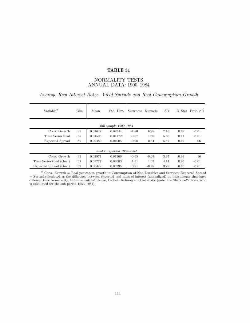
TABLE 31

NORMALITY TESTSANNUAL DATA: 1900–1984

Average Real Interest Rates, Yield Spreads and Real Consumption Growth

Variablea Obs. Mean Std. Dev. Skewness Kurtosis SR D–Stat Prob.>D


Cons. Growth 85 0.01647 0.02344 -1.80 6.98 7.16 0.12 <.01

Time Series Real 85 0.01596 0.04172 -0.07 1.58 5.80 0.14 <.01

Expected Spread 85 0.00480 0.01005 -0.08 0.64 5.42 0.09 .06


Cons. Growth 32 0.01971 0.01269 -0.65 -0.03 3.97 0.94 .16

Time Series Real (Gov.) 32 0.02277 0.02003 1.31 1.67 4.14 0.85 <.01

Expected Spread (Gov.) 32 0.00472 0.00295 0.81 -0.28 3.75 0.90 <.01

a Cons. Growth = Real per capita growth in Consumption of Non-Durables and Services, Expected Spread= Spread calculated as the difference between expected real rates of interest (annualized) on instruments that havedifferent time to maturity. SR=Studentized Range, D-Stat=Kolmogorov D-statistic (note: the Shapiro-Wilk statisticis calculated for the sub-period 1953–1984).

111

APPENDIX E

SUPPLEMENTARY FIGURES

112

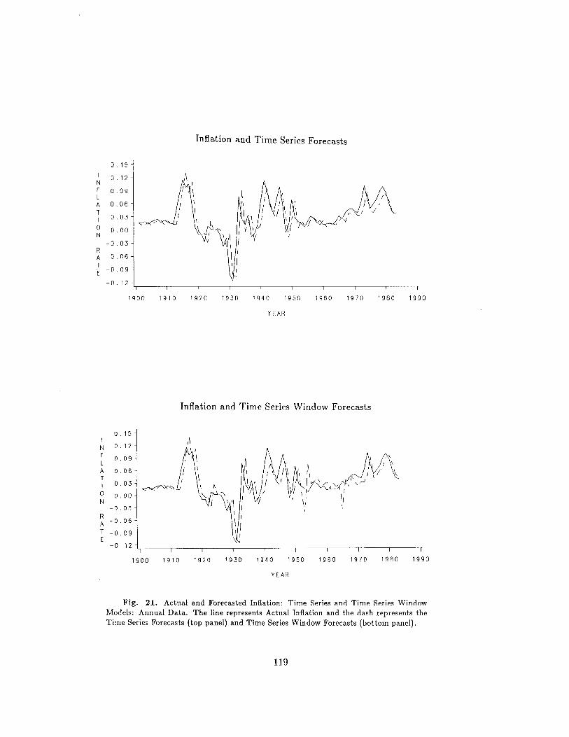
REFERENCES

Board of Governors of the Federal Reserve Board, Federal Reserve Bulletin, variousissues.

Breeden, Douglas T., 1979, “An Intertemporal Asset Pricing Model with StochasticConsumption and Investment Opportunities,” Journal of Financial Economics,7, 265–296.

Breeden, Douglas T., 1986, “Consumption, Production and Interest Rates: A Synthe-sis,” Journal of Financial Economics, 16, 3–39.

Breeden, Douglas T., and Litzenberger, R. H., 1978, “Prices of State-Contingent ClaimsImplicit in Options Prices,” Journal of Business, 51, 621–652.

Breeden, Douglas T., Michael R. Gibbons and Robert H. Litzenberger, 1985, “EmpiricalTests of the Consumption Based CAPM,” Unpublished working paper (FuquaSchool of Business, Duke University, Durham, NC).

Brown, David P. and Michael R. Gibbons, “A Simple Econometric Approach for UtilityBased Asset Pricing Models,” Journal of Finance, 40, 359–381.

Brock, William A., 1982, “Asset Prices in a Production Economy” in: The Economicsof Information and Uncertainty (University of Chicago Press, for the NBER,Chicago, IL).

Chistiano, Lawerence J., 1984, “The Effects of Aggregation over Time on Tests of theRepresentative Agent Model of Consumption,” Unpublished working paper (Grad-uate School of Business, University of Chicago, Chicago, IL).

Cox, John C., Jonathan E. Ingersoll and Stephen A. Ross, 1981, “A Re-examination ofthe Traditional Hypotheses about the Term Structure of Interest Rates,” Journalof Finance, 36, 769–799.

Cox, John C., Jonathan E. Ingersoll and Stephen A. Ross, 1985a, “An IntertemporalGeneral Equilibrium Model of Asset Prices,” Econometrica, 53, 363–384.

Cox, John C., Jonathan E. Ingersoll and Stephen A. Ross, 1985b, “A Theory of theTerm Structure of Interest Rates,” Econometrica, 53, 385–399.

Dickey, David A. and Wayne A. Fuller, 1981, “Likelihood Ratio Statistics for Autore-gressive Time Series with a Unit Root,” Econometrica, 49, 1057–1072.

Dunn, Kenneth B. and Kenneth G. Singleton, 1985, “Modeling the Term Structure of In-terest Rates Under Non-Separable Utility and Durability of Goods,” Unpublishedworking paper (Graduate School of Industrial Management, Carnegie–Mellon Uni-versity, Pittsburg, PA).

121

Fama, Eugene F., 1970, “Multiperiod Consumption-Investment Decisions,” AmericanEconomic Review, 60, 163–65.

Fama, Eugene F., 1976, Foundations of Finance (Basic Books, New York, NY).

Fama, Eugene F., 1984, “The Information in the Term Structure,” Journal of FinancialEconomics, 13, 509–528.

Fama, Eugene F., 1984, “Term Premiums in Bond Returns,” Journal of Financial Eco-nomics, 13, 529–546.

Fama, Eugene F., 1985, “Term Premiums and Default Premiums in Money Markets,”Unpublished working paper (Graduate School of Business, University of Chicago,Chicago, IL).

Fama, Eugene F., and Michael R. Gibbons, 1984, “A Comparison of Inflation Forecasts,”Journal of Monetary Economics, 13, 327–348.

Ferson, Wayne E., 1983, “Expectations of Real Interest Rates and Aggregate Con-sumption: Empirical Tests,” Journal of Financial and Quantitative Analysis, 18,477–498.

Ferson, Wayne E., and Campbell R. Harvey, 1985, “Seasonality in Consumption–BasedAsset Pricing,” Unpublished working paper (Graduate School of Business, Uni-versity of Chicago, Chicago, IL).

Ferson, Wayne E., and John J. Merrick, 1984, “Non-stationarity and Stage of theBusiness Cycle Effects in the Consumption Based Asset Pricing Relation,” Un-published working paper (Graduate School of Business, University of Chicago,Chicago, IL).

Fisher, Irving, 1907, The Rate of Interest (Macmillan, New York, NY).

Flavin, Marjorie A., 1981, “The Adjustment of Consumption to Changing Expectationsabout Future Income,” Journal of Political Economy, 89, 974–1009.

Friedman, Milton, and Anna Schwartz, 1982, Monetary Trends in the United States andthe United Kingdom (University of Chicago Press, Chicago, IL).

Grossman, Sanford, and Robert J. Shiller, 1981, “The Determinants of the Variabilityof Stock Market Prices,” American Economic Review, 71, 222–227.

Hall, Robert E., 1978, “Stochastic Implications of the Life Cycle–Permanent IncomeHypothesis: Theory and Evidence,” Journal of Political Economy, 86, 971–988.

Hall, Robert E., 1985, “Intertemporal Substitution in Consumption,” Unpublishedworking paper (Department of Economics, Stanford University, Stanford, CA).

Hall, Robert E., 1986, “Consumption” in Handbook of Modern Business Cycle Theory,Robert J. Barro (ed.), in press.

Hansen, Lars P., 1982, “Large Sample Properties of Generalized Method of MomentEstimators,” Econometrica, 50, 1029–1054.

122

Hansen, Lars P., 1985, “Econometric Modeling of Asset Pricing Under Rational Ex-pectations,” Unpublished working paper (Department of Economics, Universityof Chicago, Chicago, IL).

Hansen, Lars P., 1986, “Unpublished Lecture Notes from Estimation and Inference forDynamic Econometric Models I and II” (Department of Economics, University ofChicago, Chicago, IL).

Hansen, Lars P., and Kenneth J. Singleton, 1982, “Generalized Instrumental VariablesEstimation of Nonlinear Rational Expectations Models,” Econometrica, 50, 1269–1285.

Hansen, Lars P., and Kenneth J. Singleton, 1983, “Stochastic Consumption, Risk Aver-sion, and the Temporal Behavior of Asset Returns,” Journal of Political Economy,91, 249–265.

Hansen, Lars P., and Kenneth J. Singleton, 1984, “Errata,” Econometrica, 52, 267–268.

Harvey, Campbell R., 1984, “Yield Spreads, Stock Returns and Real Activity,” Un-published working paper (Graduate School of Business, University of Chicago,Chicago, IL).

Homer, Sidney, 1963, A History of Interest Rates (Rutgers University Press, Newark,NY).

Keim, Donald B. and Robert F. Stambaugh, 1986, “Predicting Returns in the Stockand Bond Markets,” Unpublished working paper (Graduate School of Business,University of Chicago, Chicago, IL).

Kessel, Reuben A., 1965, The Cyclical Behavior of the Term Structure of Interest Rates(National Bureau of Economic Research, Occasional Paper 91, New York, NY).

Kuznets, Simon, 1961, Capital in the American Economy (National Bureau of EconomicResearch, New York, NY).

Litzenberger, Robert H. and Ehud I. Ronn, “A Utility-Based Model of Common StockPrice Movements,” Journal of Finance, 41, 67–92.

Lucas, Robert E. Jr., 1978, “Asset Prices in an Exchange Economy,” Econometrica, 46,1429–1445.

Macaulay, Frederick, 1938, The Movement of Interest Rates, Bond Yields and StockPrices in the United States since 1856 (National Bureau of Economic Research,New York, NY).

Mankiw, N. Gregory, 1985, “Consumer Durables and the Real Interest Rate,” Reviewof Economics and Statistics, 67, 353–362.

Mankiw, N. Gregory, Julio J. Rotemberg and Lawrence H. Summers, 1985, “Intertempo-ral Substitution in Macroeconomics,” Quarterly Journal of Economics, 225–251.

123

Miron, Jeffrey A., 1985, “Seasonal Fluctuations and the Life Cycle-Permanent IncomeModel of Consumption,” Unpublished working paper (Department of Economics,University of Michigan, Ann Arbor, MI).

McNees, Stephen K., 1985, “Root Mean Square Errors and Mean Absolute Errors,”Unpublished working paper (Federal Reserve Bank of Boston, Boston, MA).

Merton, Robert C., 1971, “Optimum Consumption and Portfolio Rules in a ContinuousTime Model,” Journal of Economic Theory, 3, 373–413.

Rubinstein, Mark, 1974, “An Aggregation Theorem for Securities Markets,” Journal ofFinancial Economics, 1, 225–244.

Rubinstein, Mark, 1976, “The Valuation of Uncertain Income Streams and the Pricingof Options,” Bell Journal of Economics, 1, 407–425.

Sargent, Thomas J., 1979, Macroeconomic Theory (Academic Press, New York, NY).

Sargent, Thomas J., 1984, “Theories of Consumption and Asset Prices,” Unpublishedworking paper (Department of Economics, University of Minnesota, Minneapolis,MN).

Seldon, Larry, 1978, “A New Representation of Preferences over ‘Certain × Uncertain’Consumption Pairs: The ‘Ordinal Certainty Equivalent’ Hypothesis,” Economet-rica, 46, 1045–1060.

Tauchen, George, 1985, “Statistical Properties of Generalized Method of Moments Es-timates of Structural Parameters Using Financial Market Data,” Unpublishedworking paper (Department of Economics, Duke University, Durham, NC).

Sims, Christopher A., 1980, “Comparison of Interwar and Postwar Business Cycles:Monetarism Reconsidered,” American Economic Review, 70, 250–257.

United States, Department of Commerce, Bureau of Economic Analysis, National In-come and Product Accounts of the United States, various issues.

United States, Department of Commerce, Long-Term Economic Growth, 1860-1970.

United States, Department of Commerce, Survey of Current Business, various issues.

United States, Department of Commerce, Bureau of the Census, Current PopulationReports, various issues.

White, Halbert, 1980, “A Heteroskedasticity-Consistent Covariance Matrix Estimatorand a Direct Test for Heteroskedasticity,” Econometrica, 48, 817–838.

124

Documents

THE UNIVERSITY OF CHICAGO RECOVERING EXPECTATIONS …charvey/Research/Thesis/Thesis.pdfthe university of chicago recovering expectations of consumption growth from an equilibrium model