The Tutte polynomial of a graph, depth-firstsearch, and simplicial complex partitions

Dedicated to Dominique Foata on the occasion of his 60th birthday

Appeared in Electronic J. Combin. (Foata Festschrift Volume), 3(1996)

Ira M. GesselDepartment of Mathematics

Brandeis UniversityWaltham, MA 02254-9110

Bruce E. SaganDepartment of MathematicsMichigan State University

East Lansing, MI 48824-1027

Key Words: Tutte polynomial, simplicial complex, partition,depth-first search, spanning tree, acyclic orientation, inversion,parking function

AMS subject classification (1985): Primary 05C30; Secondary05C05, 68R10.

Abstract

One of the most important numerical quantities that can be computed from agraph G is the two-variable Tutte polynomial. Specializations of the Tutte poly-nomial count various objects associated with G, e.g., subgraphs, spanning trees,acyclic orientations, inversions and parking functions. We show that by parti-tioning certain simplicial complexes related to G into intervals, one can providecombinatorial demonstrations of these results. One of the primary tools for pro-viding such a partition is depth-first search.

1 Introduction and definitions

Tutte defined the polynomial that bears his name as the generating function fortwo parameters, namely the internal and external activities, associated with thespanning trees of a connected graph. In this paper we will propose a number ofnew, but related, notions of external activity. We will show in the next six sec-tions that using these other definitions of activity can lead to combinatorial proofsof results about many specializations of tG. These evaluations count subgraphs,acyclic orientations, subdigraphs, inversions and parking functions. The basic ideais to use depth-first search to associate a spanning forest F with each object tobe counted. This partitions the simplicial complex of all objects (ordered by in-clusion) into intervals, one for each F . Every interval turns out to be a Booleanalgebra consisting of all ways to add externally active edges to F . Expressing theTutte polynomial in terms of sums over such intervals permits us to extract thenecessary combinatorial information.

The idea of using partitions to get information about the Tutte polynomialgoes back to Crapo [8] and has also been used by Bari [2], Dawson [9, 10], Gesseland Wang [18], Gordon and Traldi [20], and others. See Bjorner [4] for a goodaccount of the connection between Tutte polynomials, partitions, and shellability.See Brylawski [5] and his survey with Oxley [6] for the general theory of the Tuttepolynomial. Partitioning simplicial complexes into Boolean algebras also has otherapplications. See, for example, the paper of Garsia and Stanton [15]. Finally, weshould mention that Kleitman and Winston [23] have used depth-first search toconstruct a bijection in a context similar to ours. However, our paper is the first tosystematically mine the combination of the partitioning and DFS ideas to obtaina wide range of results.

Let G denote a graph with vertex set V . In most of our work (in particular, fordepth-first search and its variations) we assume that V is totally ordered. Often wewill take V = {1, 2, . . . , n}. We will permit G’s edge set to have loops and multipleedges, calling two edges with the same endpoints parallel. It will be convenient toidentify a graph with its edge set and use the notation G for both. All the previousconventions will apply to digraphs as well.

All of our subgraphs are spanning, that is, a subgraph of G has the same vertexset as G. Thus we identify subgraphs of G with subsets of the edge set. A subgraphof G is a forest if it is acyclic; in particular, it must contain no loops or paralleledges. The connected components of a forest are trees.

Before defining the Tutte polynomial, tG(x, y), we make the convention that,except where stated otherwise, G is a connected graph. This is no loss of generalityfor two reasons. First, if G is disconnected then tG(x, y) is just the product of theTutte polynomials of the components of G. Furthermore, most of the algorith-

1

mic constructions that we will use can be carried out in G by applying them toeach component. In the few places where this is not true, we will indicate whatmodifications need to be made for the general case.

Now suppose we are given G and a total ordering of its edges. Consider aspanning tree T of G. An edge e ∈ G − T is externally active if it is the largestedge in the unique cycle contained in T ∪ e. We let

EA(T ) = set of externally active edges of T

andea(T ) = |EA(T )|

where | · | denotes cardinality. Of course, the set of externally active edges dependson both G and T . However, G will always be clear from context. An edge e ∈ Tis internally active if it is the largest edge in the unique cocycle contained in(G− T ) ∪ e. (A cocycle is a minimal disconnecting subset of G.) We let

IA(T ) = set of internally active edges of T

andia(T ) = |IA(T )|.

Tutte [40] then defined his polynomial as

tG(x, y) =∑T⊆G

xia(T )yea(T ) (1)

where the sum is over all spanning trees T of G. Tutte showed that tG is well-defined, i.e., independent of the ordering of the edges of G. Henceforth, we willnot assume that the edges of G are ordered unless it is explicitly stated.

We end this section by reviewing the notion of depth-first search, which weabbreviate to DFS. Given a graph H with vertex set V , we will use the followingalgorithm to create the DFS forest F of H.

DFS1 Let F := ∅.

DFS2 Let v be the least unvisited vertex in V . Mark v as visited.

DFS3 Pick some unvisited vertex u adjacent to v by an edge e if such a vertexexists. Mark u as visited and set v := u, F := F ∪ e. Repeat this step untilv has no unvisited neighbors.

DFS4 If there is a visited vertex with unvisited neighbors, let v be the most recentlyvisited such vertex and go to DFS3. Otherwise, go to DFS2 and repeat theprocess until all vertices are visited.

The DFS variants that we will introduce in the next sections are all constructedby specifying the vertex u and the edge e in step DFS3.

2

2 Subgraphs

Let G be a graph with |V | = n, and let H be a subgraph. We denote by c(H) thenumber of components of H. We introduce two useful invariants associated withH, namely

σ(H) = c(H)− c(G) = c(H)− 1 (2)

andσ∗(H) = |H| − |V |+ c(H) = |H| − n+ c(H) (3)

where we recall that |H| denotes the number of edges in H. These quantities arenaturally associated with the cycle matroid of G whose independent sets consistof all spanning forests F of G. The rank of H ⊆ G in this matroid is

ρ(H) = max{|F | : F ⊆ H with F a spanning forest of G}= |V | − c(H)

and the corank is

ρ∗(H) = max{|C| : C ⊆ H with G− C connected}= |H| − c(G−H) + 1.

Thusσ(H) = ρ(G)− ρ(H)

andσ∗(H) = ρ∗(G)− ρ∗(G−H).

It is well known [4] that one evaluation of the Tutte polynomial is the generatingfunction for subgraphs of G with respect to the invariants σ and σ∗.

Theorem 2.1 We have

tG(1 + x, 1 + y) =∑H⊆G

xσ(H)yσ∗(H) (4)

where the sum is over all subgraphs H of G.

The version of depth-first search that will be useful in connection with sub-graphs H ⊆ G is greatest-neighbor DFS. Each time we perform DFS3 we visitthe unvisited neighbor with largest label first. (However, we still always start thesearch at the vertex with smallest label. One of the reasons for these conventionsis to coincide with those used later when discussing inversions in trees.) We alsoassume that each set of parallel edges is totally ordered and that we always take

3

r1r4r6 r2 r5r7

r8r3

��BBBBBBB

b@@@@

@@i �

�

cAAAA@@��a ��d

r1r4r6 r2 r5r7

r8r3

��

b@@@@

@@i

cAAAA@@��a

r1r4r6 r2 r5r7

r8r3

��

b@@@@

@@

c@@

G H ⊆ G F = F(H)

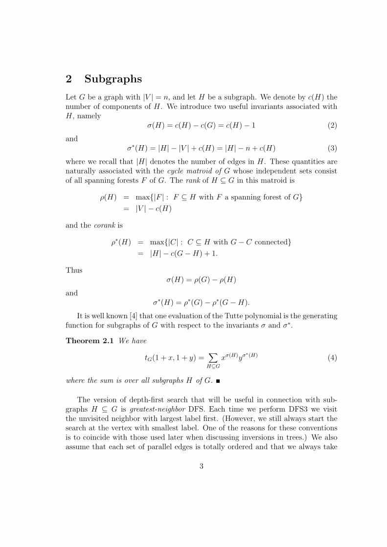
Figure 1: A greatest-neighbor DFS forest F for H ⊆ G

the largest edge connecting two vertices. If H has greatest-neighbor DFS forestF , then we write F+(H) = F which we will often abbreviate to F(H) = F . It isconvenient to root each tree of F(H) at its least vertex. We also note that F(H)does not depend on the edges of G−H and that c(F(H)) = c(H).

By way of illustration, suppose we have the graph G in Figure 1. The two setsof parallel edges are ordered lexicographically. Then the given subgraph H hasgreatest-neighbor forest F with components rooted at vertices 1 and 3.

Now given a spanning forest F ⊆ G let us say that an edge e ∈ G − F is(greatest-neighbor) externally active if

F(F ∪ e) = F.

We write E+(F ), or simply E(F ), for the set of greatest-neighbor externally activeedges. In our previous example, edges {1, 2}, {3, 7}, {2, 2} and a = {4, 6} areexternally active while {1, 5}, {5, 7} and d = {7, 8} are not.

The next result follows easily from the definitions. In it, ] stands for disjointunion.

Proposition 2.2 If H is any subgraph and F is any spanning forest of G then

F(H) = F ⇐⇒ F ⊆ H ⊆ F ] E(F ).

Thus the intervals [F, F ] E(F )] partition the simplicial complex of all subgraphsof G into Boolean algebras, one for each spanning forest.

To turn this proposition into an enumerative result, note that if F(H) = Fthen c(H) = c(F ) so σ(H) = σ(F ) = c(F )−1 and σ∗(H) = |H|−|F | = |H∩E(F )|.Thus, if we fix a forest F and sum over the corresponding interval∑

H:F(H)=F

xσ(H)yσ∗(H) = xσ(F )

∑A⊆E(F )

y|A|

4

= xσ(F )(1 + y)|E(F )|.

Summing over all forests F , we have∑H⊆G

xσ(H)yσ∗(H) =

∑F⊆G

xσ(F )(1 + y)|E(F )|.

But from Theorem 2.1, we know that the left-hand side is just tG(1 + x, 1 + y).Thus, changing y to y − 1, we have

tG(1 + x, y) =∑F⊆G

xσ(F )y|E(F )|

orx tG(1 + x, y) =

∑F⊆G

xc(F )y|E(F )|, (5)

an equation that will be useful in the future. Note that if G were allowed to bedisconnected then the factor of x on the left of this equation would be replacedwith xc(G).

We will now give a characterization of the edges in E(F ) that will allow us tomine more combinatorial information from equation (5). Consider a tree T in Frooted at its smallest vertex. Then we will use all the usual family tree conventionswhen talking about vertices of T (parent, child, and so on). Also, we call a pair ofvertices (u, v) in T an inversion (respectively non-inversion) if u is an ancestor ofv and u > v (respectively u < v). Finally, a cross edge is e = {u, v} where u is nota descendant of v and vice-versa.

Lemma 2.3 Suppose G is a graph with spanning forest F and e ∈ G − F . Thene ∈ E(F ) if and only if e is of one of the following types:

1. e = {u, v} where v is a descendant of u, and (w, v) is an inversion where wis the child of u on the unique u-v path in F , or

2. e < f where f ∈ F is an edge with the same endpoints as e, or

3. e is a loop.

Figure 2 shows a schematic diagram of an externally active edge correspondingto an inversion. For a concrete example, see Figure 1 where edges {1, 2} and {3, 7}are of type 1, edge a = {4, 6} is of type 2 and {2, 2} is of type 3.

Proof of Lemma 2.3. It suffices to show that F(F ∪ e) does not contain eif and only if e is one of these three types. If e is of type 1, then DFS will reachu before v. But since we are using greatest-neighbors, the search will continue to

5

rurwr r rv

����AAHH

w > v

Figure 2: The inversion case of Lemma 2.3

w regardless of the presence of {u, v}. By the time the search reaches v, u hasalready been visited and so e cannot be used in that direction either. The paralleledge case follows from using greatest edges, and loops are never in forests.

For the converse, suppose that e is not one of the three types. Then e must beof the form

i. e = {u, v} where v is a descendant of u and (w, v) is a non-inversion, wherew is the child of u on the unique u-v path in F , or

ii. e > f where f ∈ F is an edge with the same endpoints as e, or

iii. e is a cross edge.

In the first two cases, the greatest-neighbor search will be forced to traverse e thefirst time it is encountered. So e ∈ F(F ∪ e). In the third case, suppose e = {u, v}and that u is searched first in F . Then v would eventually be visited as a neighborof u in F ∪ e. Again, this forces e ∈ F(F ∪ e).

3 Orientations

If G is a graph, then an orientation O of G is a digraph obtained by assigning oneof the two possible directions to each edge of G. If e = {u, v} is an edge then thecorresponding arc will be denoted ~e with possible directions ~e = uv or ~e = vu. Forenumerative purposes, we also consider each loop to have two possible directions.A suborientation of G is an orientation of a subgraph of G. A digraph is acyclicif it contains no directed cycles. Loops and oppositely directed parallel edges areconsidered cycles.

We can use the Tutte polynomial and DFS to count acyclic suborientations ofG. Given any digraph D, we use least-neighbor search, which goes to the smallestvertex at each step. If there are parallel arcs between the two vertices, they are

6

r1r3 r5 r7 r8 r6r4r

2����

�

-���

6����

�

@@I - i

)��������?

@@I ��6

r1r3 r5 r7 r8 r6r4r

2����

�

6����

�

�����?

D F

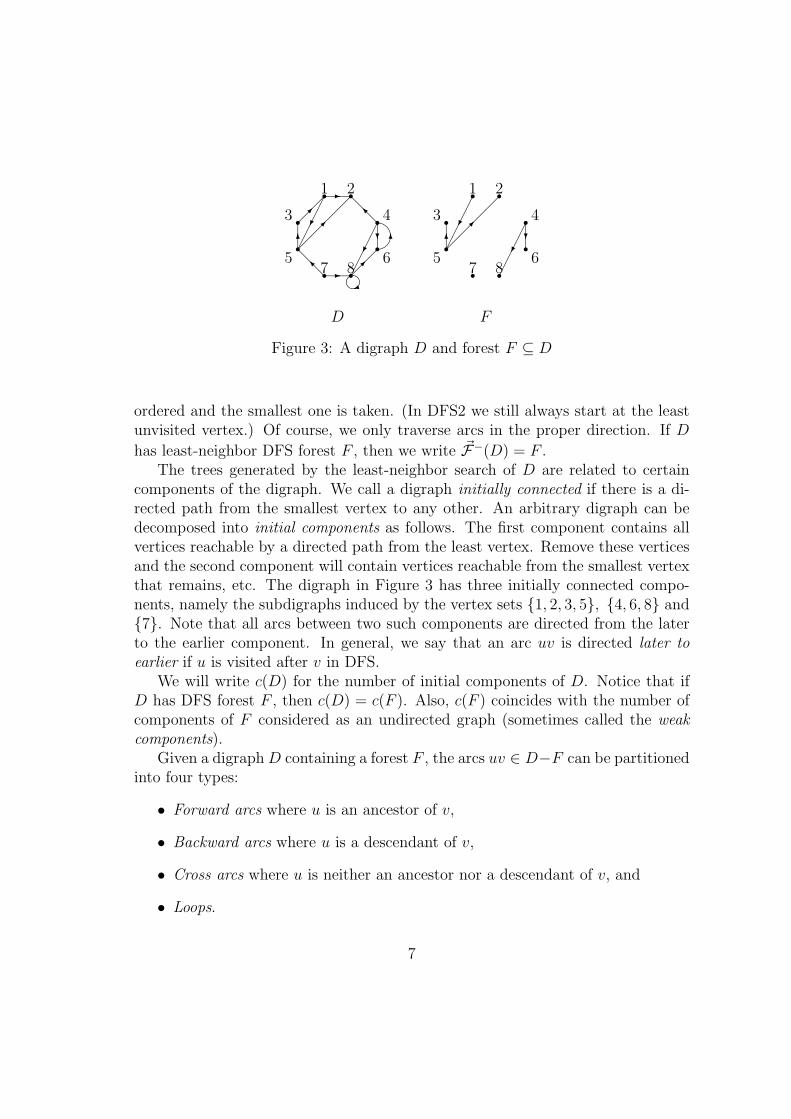
Figure 3: A digraph D and forest F ⊆ D

ordered and the smallest one is taken. (In DFS2 we still always start at the leastunvisited vertex.) Of course, we only traverse arcs in the proper direction. If D

has least-neighbor DFS forest F , then we write ~F−(D) = F .The trees generated by the least-neighbor search of D are related to certain

components of the digraph. We call a digraph initially connected if there is a di-rected path from the smallest vertex to any other. An arbitrary digraph can bedecomposed into initial components as follows. The first component contains allvertices reachable by a directed path from the least vertex. Remove these verticesand the second component will contain vertices reachable from the smallest vertexthat remains, etc. The digraph in Figure 3 has three initially connected compo-nents, namely the subdigraphs induced by the vertex sets {1, 2, 3, 5}, {4, 6, 8} and{7}. Note that all arcs between two such components are directed from the laterto the earlier component. In general, we say that an arc uv is directed later toearlier if u is visited after v in DFS.

We will write c(D) for the number of initial components of D. Notice that ifD has DFS forest F , then c(D) = c(F ). Also, c(F ) coincides with the number ofcomponents of F considered as an undirected graph (sometimes called the weakcomponents).

Given a digraph D containing a forest F , the arcs uv ∈ D−F can be partitionedinto four types:

• Forward arcs where u is an ancestor of v,

• Backward arcs where u is a descendant of v,

• Cross arcs where u is neither an ancestor nor a descendant of v, and

• Loops.

7

r1r3r2 r

5r7

r8

r6r4

������

BBBBBBB

AAAA

a@@ ��b

r1r3r2 r

5r7

r8

r6r4

��

?

BBBBBBB

N?AAAA

U

�

?a@@I ��b?

r1r3r2 r

5r7

r8

r6r4

��BBBBBBB

N?AAAA

U?a

G O ⊆ G F = ~F−(O)

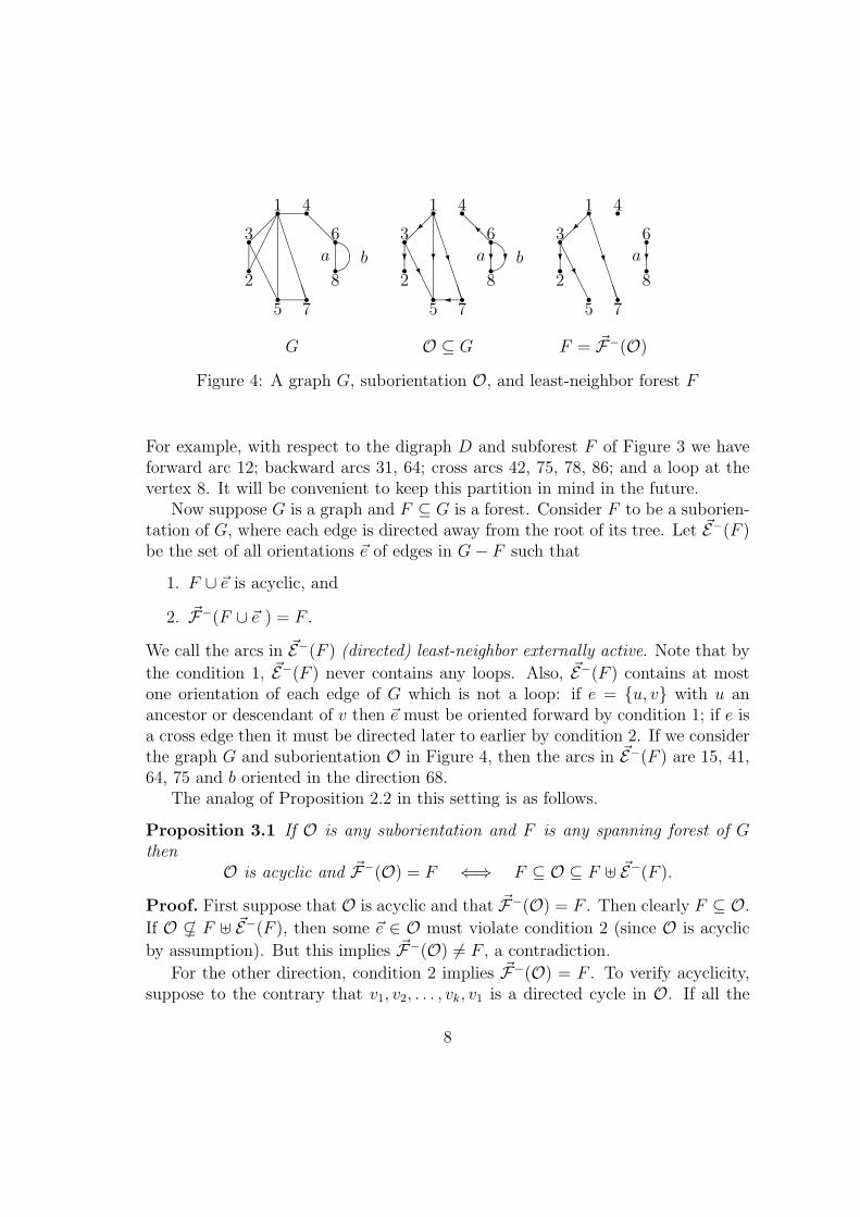
Figure 4: A graph G, suborientation O, and least-neighbor forest F

For example, with respect to the digraph D and subforest F of Figure 3 we haveforward arc 12; backward arcs 31, 64; cross arcs 42, 75, 78, 86; and a loop at thevertex 8. It will be convenient to keep this partition in mind in the future.

Now suppose G is a graph and F ⊆ G is a forest. Consider F to be a suborien-tation of G, where each edge is directed away from the root of its tree. Let ~E−(F )be the set of all orientations ~e of edges in G− F such that

1. F ∪ ~e is acyclic, and

2. ~F−(F ∪ ~e ) = F .

We call the arcs in ~E−(F ) (directed) least-neighbor externally active. Note that by

the condition 1, ~E−(F ) never contains any loops. Also, ~E−(F ) contains at mostone orientation of each edge of G which is not a loop: if e = {u, v} with u anancestor or descendant of v then ~e must be oriented forward by condition 1; if e isa cross edge then it must be directed later to earlier by condition 2. If we considerthe graph G and suborientation O in Figure 4, then the arcs in ~E−(F ) are 15, 41,64, 75 and b oriented in the direction 68.

The analog of Proposition 2.2 in this setting is as follows.

Proposition 3.1 If O is any suborientation and F is any spanning forest of Gthen

O is acyclic and ~F−(O) = F ⇐⇒ F ⊆ O ⊆ F ] ~E−(F ).

Proof. First suppose that O is acyclic and that ~F−(O) = F . Then clearly F ⊆ O.

If O ⊆/ F ] ~E−(F ), then some ~e ∈ O must violate condition 2 (since O is acyclic

by assumption). But this implies ~F−(O) 6= F , a contradiction.

For the other direction, condition 2 implies ~F−(O) = F . To verify acyclicity,suppose to the contrary that v1, v2, . . . , vk, v1 is a directed cycle in O. If all the

8

vi are on the same path from the root of some tree of F , then some cycle arc isoriented backward, contradicting the observation after the definition of ~E−(F ).

Otherwise we have a cross arc, say vkv1. We can assume that all cross arcshave endpoints in the same tree of F , since once we have left a component by across arc we can never return. Note that v1 is earlier that vk because all crossarcs are directed later to earlier. Also v1 is not an ancestor of vk by definition ofcross arc. Assume, by induction, that vi−1 is earlier than vk and not vk’s ancestor.Now vi−1vi must be either a forward or cross arc. In the former case, vi is earlierthan and not an ancestor of vk. In the latter case, vi must be earlier than vi−1

and therefore earlier than vk. Also, vi cannot be an ancestor of vk: Since vi−1viis a cross arc, every descendant of vi is earlier than vi−1, but by the inductionhypothesis vk is later than vi−1. Thus the induction hypothesis holds for vi, whichis a contradiction when i = k.

Next, we characterize the arcs in ~E−(F ) just as we did for E(F ). The proof issimilar to that of Lemma 2.3 and is left to the reader.

Lemma 3.2 Suppose G is a graph with spanning forest F and e ∈ G − F . Then~e ∈ ~E−(F ) if and only if ~e is of one of the following types:

1. ~e = uv is a forward arc, and (w, v) is a non-inversion where w is the childof u on the unique u-v path in F , or

2. ~e > ~f where ~f ∈ F is an edge with the same endpoints and orientation as ~e,or

3. ~e is a cross arc directed later to earlier.

In our previous example the arc 15 is of type 1, arc b = 68 is of type 2, and allother arcs in ~E−(F ) are of type 3.

Comparing Lemmas 2.3 and 3.2 (in particular, the conditions in the proof ofthe converse of the former and in the statement of the latter), we immediatelyobtain a corollary.

Corollary 3.3 Suppose G is a graph with spanning forest F . Then

|G| = |F |+ |E(F )|+ |~E−(F )|.

We are now ready to count suborientations by initial components and numberof edges. If we did not assume that G was connected, the factor of xyn−1 on theright side of the following equation would be replaced by xc(G)yn−c(G).

9

Theorem 3.4 If G has n vertices, then

∑Oxc(O)y|O| = xyn−1(1 + y)σ

∗(G) tG

(1 + x+

x

y,

1

1 + y

)(6)

where the sum is over all acyclic suborientations of G.

Proof. Using Proposition 3.1, Corollary 3.3, and the fact that |F | = n− c(F ) forany spanning forest F ⊆ G,∑

~F−(O)=F

xc(O)y|O| = xc(F )y|F |∑

A⊆~E−(F )

y|A|

= xc(F )y|F |(1 + y)|~E−(F )|

= xc(F )y|F |(1 + y)|G|−|F |−|E(F )|

= xc(F )yn−c(F )(1 + y)|G|−n+c(F )−|E(F )|

= yn(1 + y)|G|−n(x(1 + y)

y

)c(F ) (1

1 + y

)|E(F )|

.

Summing over all F , we obtain from equation (5),

∑Oxc(O)y|O| = yn(1 + y)|G|−n

x(1 + y)

ytG

(1 +

x(1 + y)

y,

1

1 + y

)

which agrees with (6).

We can rewrite this theorem using the same invariants as for subgraphs. Forany digraph D on n vertices, let

σ(D) = c(D)− 1

andσ∗(D) = |D| − n+ c(D).

Now replace x by xy in equation (6)

∑Oxc(O)y|O|+c(O) = xyn(1 + y)σ

∗(G) tG

(1 + xy + x,

1

1 + y

)

or ∑Oxσ(O)yσ

∗(O) = (1 + y)σ∗(G) tG

(1 + x+ xy,

1

1 + y

)(7)

10

Several special cases are of interest.To count acyclic suborientations O by edges without regard to the number of

initial components, we set x = 1 in (6) and obtain

∑Oy|O| = yn−1(1 + y)σ

∗(G) tG

(2 +

1

y,

1

1 + y

).

Similarly, setting x = 1 in (7) we get

∑Oyσ∗(O) = (1 + y)σ

∗(G) tG

(2 + y,

1

1 + y

).

In particular,

2σ∗(G) tG

(3,

1

2

)= number of acyclic suborientations of G.

On the other hand, counting such orientations by number of initial componentsis done by putting y = 1 in (6):∑

Oxc(O) = x2σ

∗(G) tG

(1 + 2x,

1

2

).

To count those O for which c(O) = 1, i.e., those which are initially connected, weput x = 0 in (7) and obtain

∑c(O)=1

y|O| = yn−1(1 + y)σ∗(G) tG

(1,

1

1 + y

).

In particular,

2σ∗(G) tG

(1,

1

2

)= number of initially connected acyclic suborientations of G.

Finally, to count acyclic orientations of G, i.e., those O with |O| = |G|, wedivide (6) by y|G| and take y →∞. The result is∑

|O|=|G|xc(O) = x tG (1 + x, 0) . (8)

In particular,

tG(2, 0) = number of acyclic orientations of G, and

tG(1, 0) = number of initially connected acyclic orientations of G.

This interpretation of tG(2, 0) was found by Stanley in [38], while Greene andZaslavsky [21] discovered the one for tG(1, 0). These authors expressed their resultsin terms of chromatic polynomials.

11

4 Subdigraphs

Let G be a graph. A directed subgraph or subdigraph of G is a digraph D thatcontains up to one copy of each orientation of every edge of G. Thus we permit bothorientations of an edge (including loops) to appear in a subdigraph, as opposed toa suborientation where only one is permitted.

We now consider greatest-neighbor DFS on the set of all subdigraphs of G. Theonly difference from the subgraph case is that now we are constrained to followthe directions on the arcs. If digraph D has greatest-neighbor forest F, we write~F+(D) = F . There is also the set ~E+(F ) of (directed) greatest-neighbor externally

active orientations ~e of edges of G such that ~F+(F ]~e ) = F . Notice that becauseof the disjoint union, we have ~e ∈/ F . However, if uv ∈ F then we always have

vu ∈ ~E+(F ).The next four results are similar to those we have seen in the previous sections,

so we will only indicate a proof of the third. In what follows, if F is a forest thenan E-active edge is an edge e in E(F ), i.e., e is greatest-neighbor externally activein the undirected sense. All other edges of G− F will be called E-passive.

Proposition 4.1 If D is any subdigraph and F is any spanning forest of G then

~F+(D) = F ⇐⇒ F ⊆ D ⊆ F ] ~E+(F ).

Lemma 4.2 Suppose G is a graph with spanning forest F . Then ~e ∈ ~E+(F ) ifand only if ~e is of one of the following types:

1. e is an E-active arc directed forward.

2. e is any arc of G directed later to earlier.

Corollary 4.3 Suppose G is a graph with spanning forest F . Then

|G| = |~E+(F )| − |E(F )|.

Proof. The edges of G can be partitioned into those in F , those that are E-activeand those that are E-passive. The following table lists the number of times eachsort of edge is counted in ~E+(F ) and E(F ).

edges ~E+(F ) E(F )F 1 (backward) 0E-active 2 (forward and backward) 1E-passive 1 (later to earlier) 0

12

Since the net difference is 1 in each case, the result follows.

Theorem 4.4 If G has n vertices, then

∑D

xc(D)y|D| = xyn−1(1 + y)|G| tG

(1 +

x

y, 1 + y

)(9)

and ∑D

xσ(D)yσ∗(D) = (1 + y)|G| tG (1 + x, 1 + y) (10)

where the sum is over all subdigraphs of G.

As special cases, we can count subdigraphs by edges or σ∗ invariant:

∑D

y|D| = yn−1(1 + y)|G| tG

(1 +

1

y, 1 + y

)= (1 + y)2|G|

∑D

yσ∗(D) = (1 + y)|G| tG (2, 1 + y)

2|G| tG(2, 2) = number of subdigraphs of G = 4|G|,

or by number of initial components:∑D

xc(D) = x2|G| tG (1 + x, 2)∑c(D)=1

y|D| = yn−1(1 + y)|G| tG (1, 1 + y)

2|G| tG(1, 2) = number of initially connected subdigraphs of G.

From equations (4) and (10), we see that∑D

xσ(D)yσ∗(D) = (1 + y)|G|

∑H⊆G

xσ(H)yσ∗(H).

This equality can also be proved directly by exhibiting a 2|G|-to-1 map from sub-digraphs D of G to subgraphs H ⊆ G that preserves the appropriate invariantsas follows: From Lemma 4.2, D can be represented by a triple (F,E,A) where

F = ~F+(D), E is the set of directed E-active edges in D, and A is the rest of thearcs of D (so the corresponding edges could be an arbitrary subset of G). Similarly,Lemma 2.3 shows that H can be represented by a pair (F,E) where F = F+(H)and E is the set of E-active edges in H. It is easy to verify that the projectionmap

(F,E,A)→ (F,E)

(where we change arcs to edges in the image) has the desired properties.

13

5 Complete graphs

We will now show how our results on orientations and subdigraphs can be combinedwith the generating function for the Tutte polynomial of a complete graph to obtainvarious new generating functions, some of which generalize results already in theliterature. For brevity, let tn(x, y) = tKn(x, y). Tutte [41, equation (17)] obtainedan equation equivalent to the following which can be derived using the exponentialformula.

Theorem 5.1 The Tutte polynomial of the complete graph has exponential gener-ating function

∑n≥1

tn(x, y)un

n!=

1

x− 1

∑n≥0

y(n2)(y − 1)−nun

n!

(x−1)(y−1)

− 1

.Next we find the generating function for acyclic digraphs, which are just acyclic

suborientations O ⊆ Kn. To do this, it will be convenient to define the graphicgenerating function of a sequence (an)n≥0 to be∑

n≥0

anun

(1 + y)(n2)n!

.

According to equation (6), the count of acyclic digraphs on n vertices by numberof arcs and initial components is given by

an(x, y)def=

∑O⊆Kn

xc(O)y|O| = xyn−1(1 + y)(n−1

2 ) tn

(1 + x+

x

y,

1

1 + y

).

Applying the previous theorem yields

∑n≥1

an(x, y)

yn(1 + y)(n−1

2 )

un

n!=

x

y

1

x+ xy

∑n≥0

1

(1 + y)(n2)

(−y

1 + y

)−nun

n!

(x+xy

)( −y1+y

)

− 1

=

1

1 + y

∑n≥0

(−1)n(1 + y)n

ynun

(1 + y)(n2)n!

−x −1

. (11)

If we define a0(x, y) = 1 and replace u by yu1+y

, then this last result simplifies.

Corollary 5.2 The graphic generating function for acyclic digraphs is

∑n≥0

an(x, y)un

(1 + y)(n2)n!

=

∑n≥0

(−1)nun

(1 + y)(n2)n!

−x .

14

Stanley [38] and Robinson [35] obtained this result when x = y = 1, as didLiskovets [29] and Rodionov [36] when x = 1. When x and y are integers withy ≥ 0, Stanley also gives an interpretation to these graphic generating functions interms of the theory of posets of full binomial type developed by himself, Doubiletand Rota [11].

We can derive the generating function for initially connected acyclic digraphscounted by number of arcs using

cn(y)def=

an(x, y)

x

∣∣∣∣∣x=0

.

Dividing equation (11) by x and letting x→ 0 yields the desired formula.

Corollary 5.3 The graphic generating function for initially connected acyclic di-graphs is

∑n≥1

cn(y)un

(1 + y)(n2)n!

= ln

∑n≥0

(−1)nun

(1 + y)(n2)n!

−1

.

Putting together these last two theorems, we see that

∑n≥0

an(x, y)un

(1 + y)(n2)n!

= exp

x∑n≥1

cn(y)un

(1 + y)(n2)n!

This is a special case of a more general exponential formula for digraphs whichdoes not seem to have been stated before.

Theorem 5.4 (Exponential formula for digraphs) Let D be a class of ini-tially connected labeled digraphs with the property that an order-preserving changeof labels does not affect membership in D. Let cn(y) count digraphs in D on thelabel set {1, 2, . . . , n} by number of arcs. Then

exp

x∑n≥1

cn(y)un

(1 + y)(n2)n!

=∑

k,m,n≥0

bk,m,n xkym

un

(1 + y)(n2)n!

(12)

where bk,m,n is the number of digraphs on {1, 2, . . . , n} with m arcs, k initial com-ponents, and every such component in D.

Proof. Taking the coefficient of xkun on both sides of equation (12), it suffices toshow

1

(1 + y)(n2)n!

∑m≥0

bk,m,n ym =

1

k!

∑n1+···+nk=n

k∏i=1

cni(y)

(1 + y)(ni2 )ni!

15

where the sum is over all ordered partitions of n. Equivalently

∑m≥0

bk,m,n ym =

1

k!

∑n1+···+nk=n

(n

n1, . . . , nk

)cn1(y) · · · cnk(y) (1 + y)

∑i<j

ninj

The left side of this formula just counts digraphs D on n vertices with k initialcomponents by number of arcs. But the right sums to the same thing. Themultinomial coefficient counts the number of ways to partition the vertices ofD into k ordered subsets for the initial components. Summing over all orderedpartitions of n and then dividing by k! gives coefficients which count unorderedpartitions of the vertices. The cni(y) give the arc count for each component. Andthe power of 1 + y accounts for the arcs between components which must all bedirected from a later to an earlier component.

A general theory of exponential formulas has been developed by Stanley [39],but this result does not seem to be a consequence. In the example we have beenconsidering, the set D consists of all initially connected acyclic digraphs.

As a further demonstration, we can count digraphs without the acyclicity con-dition. Let dn(x, y) =

∑D x

c(D)y|D| (respectively, en(y) =∑D y|D|) where the sum

is over all digraphs (respectively, all initially connected digraphs) on n vertices.The graphic generating function for all digraphs by number of arcs is∑

n≥0

(1 + y)2(n2) un

(1 + y)(n2)n!

=∑n≥0

(1 + y)(n2)u

n

n!

Using our Exponential Formula, we immediately get the following result.

Corollary 5.5 The graphic generating function for dn(x, y) is

∑n≥0

dn(x, y)un

(1 + y)(n2)n!

=

∑n≥0

(1 + y)(n2)u

n

n!

x .The graphic generating function for en(y) is

∑n≥1

en(y)un

(1 + y)(n2)n!

= ln

∑n≥0

(1 + y)(n2)u

n

n!

.

6 Neighbors-first search

A specialization of tn(x, y) that has received some attention is tn(y)def= tn(1, y).

Mallows and Riordan [30] first studied this polynomial as the inversion enumer-ator for trees. See also the book of Foata [12, pp. 144–147] and the papers of

16

Gessel, Sagan and Yeh [19] and Gessel [17]. Kreweras [28] has given a numberof other interpretations to this polynomial which have been further studied byMoszkowski [31]. See also Beissinger [3], who gives a bijective proof that tn(1, y)counts inversions. In Section 9 we will give a table of these polynomials.

For completeness, we state the connection with the inversion polynomial. Itfollows directly from Lemma 2.3 applied to G = Kn.

Proposition 6.1 If T is a tree, let inv T stand for the number of inversions of T .Then

tn(y) =∑T

yinv T

where the sum is over all trees with n vertices.

We will now give another interpretation of tn(y) using a modified version ofDFS which is sometimes called neighbors-first search or NFS (see [7, p. 154]). Thefollowing steps are applied to a graph H to build an NFS forest F . Note thatmarking and searching a vertex are now two separate actions.

NFS1 Let F = ∅.

NFS2 Let v be the least unmarked vertex in V and mark v.

NFS3 Search v by marking all neighbors of v that have not been marked and addingto F all edges from v to theses vertices.

NFS4 Recursively search all the vertices marked in NSF3 in increasing order, stop-ping when every vertex that has been marked has also been searched.

NSF5 If there are unmarked vertices, then return to NSF2. Otherwise, stop.

Thus NFS searches nodes in a depth-first manner but marks children in a locallybreadth-first manner. In choosing the vertex u in NFS2, we will always pick theone with smallest label and use the smallest ordered edge. Denote the resultingforest by F = FN(H). As an example, for the graph H in Figure 5 we start atvertex 1, designating 3 and 4 as its children. Next we search node 3 and mark 5, 6and 8 as its offspring. Note that 4 cannot be a child of 3 since it is already a childof 1. The search now continues at 5, and so forth.

Observe that traversing a forest F by NFS gives a linear ordering to the childrenof each vertex, i.e., the order in which we search them from smallest to largest label.We will display this as a left-to-right order of the siblings when we draw F in theplane and use corresponding terminology.

17

r1r3 r4r5 r6 r8 r2r7

������������

@@@

�����

�������

r1r3 r4r5 r6 r8 r2r7

������������

@@@

H F = FN(H)

Figure 5: A graph H and NSF forest F

As usual, given a spanning forest F of a graph G, we define EN(F ), the set ofedges externally active with respect to NFS, to be those edges e in G−F such that

FN(F ∪ e) = F.

The next set of results should be easy for the reader to prove by mimicking whatwe did in Section 2. Proofs are therefore omitted.

Proposition 6.2 If H is any subgraph and F is any spanning forest of G then

FN(H) = F ⇐⇒ F ⊆ H ⊆ F ] EN(F ).

Proposition 6.3 If G is a connected graph, then

tG(1 + x, y) =∑F⊆G

xσ(F )y|EN (F )|

where the sum is over all spanning forests of G. In particular

tn(y) =∑T

y|EN (T )| (13)

where the sum is over all trees on n vertices.

Theorem 6.4 Suppose G is a graph with spanning forest F and e ∈ G−F . Thene ∈ EN(F ) if and only if e is of one of the following types:

1. e = {u, v} where v is a descendant of u’s parent, and w < u where w is thesibling of u on the unique path from their parent to v in F , or

18

rrwr r rv

ru��HH

��AAHH

��

��

��

w < u

Figure 6: The first case of Theorem 6.4

2. e > f where f ∈ F is an edge with the same endpoints as e, or

3. e is a loop.

Since our applications will all be to G = Kn, only the first of these three casesreally matters. A schematic diagram of this case is given in Figure 6.

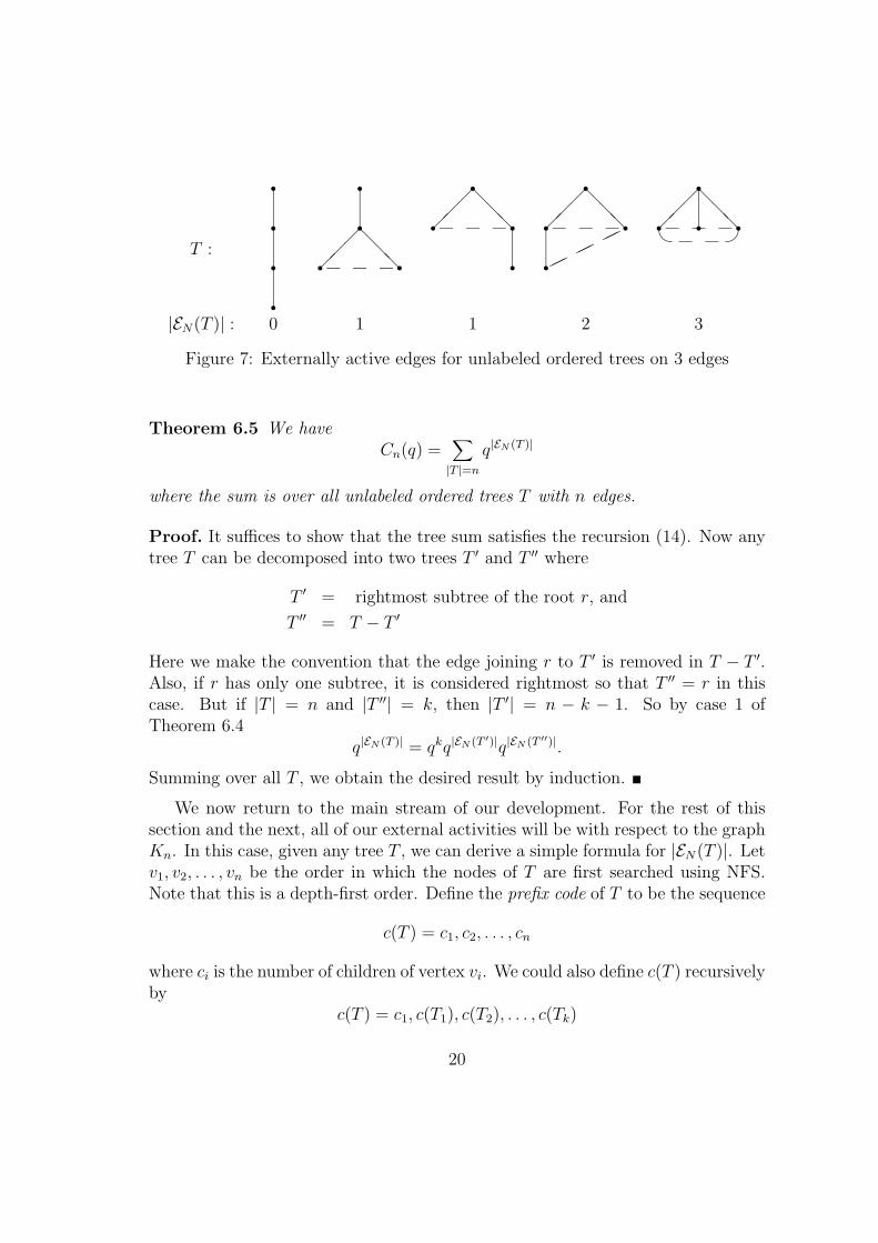
It follows from Propositions 6.1 and 6.3 that the distribution of |EN(T )| forlabeled NFT trees is the same as that for inv T . We digress briefly to note thatthe the distribution of external activities for unlabeled ordered trees is given bythe q-Catalan numbers studied by Andrews [1], Furlinger and Hofbauer [14], andKrattenthaler [27]. Any unlabeled ordered tree can be given an NFT labeling bylabeling the root as 1 and then making sure that the labels on the children ofevery vertex increase from left to right. Thus we can let the external activity of anunlabeled tree T be the external activity of any NFT labeling of T as a spanningtree of a complete graph. Now define polynomials Cn(q) by C0(q) = 1 and

Cn(q) =n−1∑k=0

qkCk(q)Cn−k−1(q). (14)

The first few values are

C0(q) = C1(q) = 1, C2(q) = 1 + q, C3(q) = 1 + 2q + q2 + q3,

C4(q) = 1 + 3q + 3q2 + 3q3 + 2q4 + q5 + q6.

If we compute the external activities of the unlabeled ordered trees on 3 edges (seeFigure 7), then we obtain∑

|T |=3

q|EN (T )| = 1 + 2q + q2 + q3.

This is evidence for the next theorem.

19

T :

rrrr

rrr r���

@@@

rr rr

���

@@@

rr rr���

@@@��

����

rr r r���

@@@ �

|EN(T )| : 0 1 1 2 3

Figure 7: Externally active edges for unlabeled ordered trees on 3 edges

Theorem 6.5 We haveCn(q) =

∑|T |=n

q|EN (T )|

where the sum is over all unlabeled ordered trees T with n edges.

Proof. It suffices to show that the tree sum satisfies the recursion (14). Now anytree T can be decomposed into two trees T ′ and T ′′ where

T ′ = rightmost subtree of the root r, and

T ′′ = T − T ′

Here we make the convention that the edge joining r to T ′ is removed in T − T ′.Also, if r has only one subtree, it is considered rightmost so that T ′′ = r in thiscase. But if |T | = n and |T ′′| = k, then |T ′| = n − k − 1. So by case 1 ofTheorem 6.4

q|EN (T )| = qkq|EN (T ′)|q|EN (T ′′)|.

Summing over all T , we obtain the desired result by induction.

We now return to the main stream of our development. For the rest of thissection and the next, all of our external activities will be with respect to the graphKn. In this case, given any tree T , we can derive a simple formula for |EN(T )|. Letv1, v2, . . . , vn be the order in which the nodes of T are first searched using NFS.Note that this is a depth-first order. Define the prefix code of T to be the sequence

c(T ) = c1, c2, . . . , cn

where ci is the number of children of vertex vi. We could also define c(T ) recursivelyby

c(T ) = c1, c(T1), c(T2), . . . , c(Tk)

20

where T1, T2, . . . , Tk are the subtrees of v1 listed in order of increasing labels oftheir roots. For example, the nodes of the tree in Figure 5 are searched in theorder

v1, v2, . . . , v8 = 1, 3, 5, 7, 6, 8, 4, 2 (15)

which gives it prefix code

c1, c2, . . . , c8 = 2, 3, 1, 0, 0, 0, 1, 0.

Theorem 6.6 If T is a tree with prefix code c1, c2, . . . , cn then

|EN(T )| = (c1 − 1) + (c1 + c2 − 2) + · · ·+ (c1 + c2 + · · ·+ cn−1 − n+ 1)

= (n− 1)c1 + (n− 2)c2 + · · ·+ cn−1 −(n

2

)

Using our previous example

n−1∑k=1

(n− k)ck −(n

2

)= 7 · 2 + 6 · 3 + 5 · 1 + 4 · 0 + 3 · 0 + 2 · 0 + 1 · 1−

(8

2

)= 10

while

EN(T ) = {{4, 3} {4, 5} {4, 6} {4, 7} {4, 8} {6, 5} {6, 7} {8, 5} {8, 6} {8, 7}}

which has 10 elements.Proof of Theorem 6.6. It suffices to show that the term c1 + c2 + · · ·+ ci− i

counts all externally active edges whose left end is vi+1. We will do this by inductionon i. This is clearly true for i = 0. For i > 0, we distinguish two cases.

If ci > 0, then vi+1 is the leftmost child of vi. Now {vi, u} active implies thatso is {vi+1, u} (Theorem 6.4), yielding c1 + c2 + · · ·+ ci−1− i+ 1 edges. Also, thereare active edges from vi+1 to each of its siblings, for ci − 1 more edges. These arethe only active edges and the total is correct.

If ci = 0, then vi is a leaf and we get to vi+1 by backtracking. But then vi+1

was the leftmost of all the vertices joined to vi by externally active edges. So vi+1

has exactly one less (= ci − 1) active edge than vi did. Thus we are finished byinduction.

We can use the NFS interpretation of tn(y) to give a combinatorial proof of anidentity for its generating function first proved by other means in [16].

21

Theorem 6.7 Let

J(u) =∑n≥0

tn+1(y)un

n!

then

J(u) =∑n≥0

y(n2)J(u)J(yu) · · · J(yn−1u)un

n!

Proof. Taking the coefficient of un

n!on both sides, we get the equivalent statement

tn+1(y) =∑k≥0

n1+···+nk+k=n

y(k2)[y(k−1)n1tn1+1(y)

] [y(k−2)n2tn2+1(y)

]· · · n!

n1!n2! · · ·nk!k!

=∑k≥0

n1+···+nk+k=n

(n

k, n1, n2, . . . , nk

)tn1+1(y)tn2+1(y) · · · y

∑k

i=1(k−i)(ni+1).

where the factor involving tni+1(y) comes from J(yk−iu).To see that this last expression enumerates trees T by externally active edges,

consider the subtrees T1, T2, . . . , Tk of the root of T . Suppose these trees have rootsw1, w2, . . . , wk and n1, n2, . . . , nk other vertices respectively. Then the multinomialcoefficient counts the number of ways to pick the roots and then the other sets ofvertices.

The active edges {v, w} are of two types:

• edges where v and w are in the same Ti, and

• edges where v ∈ Ti and w = wj for some i < j

Edges of the first sort are accounted for by tn1+1(y)tn2+1(y) · · · tnk+1(y) while thoseof the second are taken care of by the power of y.

We end with a characterization of forests in terms of prefix codes that will helpus in Section 7. Since it is well known we omit the proof.

Theorem 6.8 The sequence c1, c2, . . . , cn is a prefix code for a tree if and only if

1.j∑i=1

(ci − 1) ≥ 0 for j < n, and

2.n∑i=1

(ci − 1) = −1

22

Notice that the preceding conditions could be rewritten as

j∑i=1

ci ≥ j for j < n, and

n∑i=1

ci = n− 1.

We can make the characterization in Theorem 6.8 even stronger by using parentfunctions. Suppose we are given a tree T having vertices {1, . . . , n} and NFS orderv1 = 1, v2, . . . , vn. The corresponding parent function is p : {2, . . . , n} → {1, . . . , n}defined by p(i) = j if the vertex labeled i has parent vj. Returning to the tree inFigure 5 with NFS order given by (15), we see that it has parent function

p(2) = 7, p(3) = 1, p(4) = 1, p(5) = 2, p(6) = 2, p(7) = 3, p(8) = 2.

Observe that |p−1(j)| = cj. This should motivate the following result whoseproof, since it follows easily from the previous theorem, is omitted.

Corollary 6.9 The function p : {2, . . . , n} → {1, . . . , n} is a parent function fora tree if and only if

|p−1(1) ∪ p−1(2) ∪ · · · ∪ p−1(j)| ≥ j for j < n

7 Hashing and parking functions

We now describe an application of tn(y) to hash coding, which is a method forstoring and retrieving data efficiently. Knuth [24, Chapter 6] gives a comprehensiveaccount of storage and retrieval methods, and in particular of hash coding (Section6.4). The hashing technique we discuss here is called “open addressing with linearprobing.” It was analyzed earlier by Knuth in [25]. We consider only the storageaspect; retrieval is similar and is discussed in detail by Knuth.

Suppose we have m boxes labeled 1 to m, and n < m objects labeled 1 to nwhich are to be put into the boxes. Each object i has a preferred box h(i), wherethe function h is called a hash function. We now insert the objects in the order 1,2, . . . , n into the boxes. When we insert object i, we place it into box h(i) if thisbox is empty. Otherwise, we probe boxes h(i) + 1, h(i) + 2, . . . in turn and placeobject i into the first empty box we find. Box numbers are taken modulo m, sothat box 1 is probed after box m. Since there are more boxes than objects, everyobject will eventually be placed into a box. Given a hash function h, which maybe an arbitrary function from {1, 2, . . . , n} to {1, 2, . . . ,m}, we let B(h) be the

23

987654321

1 1

2

1

23

1

23

4

1

23

4

5

1

23

4

56

Figure 8: Open address hashing

number of times an occupied box is probed during the insertion process. (Notethat Knuth counts as a probe the box into which an object is inserted, but we donot.) By way of illustration, consider the array of m = 9 boxes in Figure 8 wherethe box numbers are given on the far left. Reading the diagram from left to rightshows the placement of n = 6 objects using the hash function

h(1) = 9, h(2) = 3, h(3) = 3, h(4) = 9, h(5) = 4, h(6) = 3.

The number of probes is

B(h) = 0 + 0 + 1 + 1 + 1 + 3 = 6.

The following lemma, which appears in [24, pp. 530–531], is very useful.

Lemma 7.1 (Rearrangement Lemma) Suppose h and g are two hash func-tions such that the sequence g(1), . . . , g(n) is a rearrangement of h(1), . . . , h(n).Then

1. the same boxes are filled in the insertion process for h and g, and

2. B(h) = B(g).

We now study the distribution of B(h) among the mn possible hash functionsh : {1, 2, . . . , n} → {1, 2, . . . ,m}, where n < m. Let Kn,m,i be the number of such hwith B(h) = i. Also, let Ln,m,i be the number of these functions with the propertythat after all n objects are inserted, box m is empty. Since all boxes are equallylikely to be empty, we have

Ln,m,i =k

mKn,m,i, (16)

24

where k = m− n is the number of empty boxes.We now examine the polynomial

Ln,m(y) =∑i≥0

Ln,m,i yi. (17)

Suppose we perform the insertions corresponding to a hash function counted byLn,m(y). Consider the sequence of boxes after completing these insertions. Thissequence can be broken up into k = m−n subsequences, each of which consists ofzero or more filled boxes followed by an empty box. Since no object will ever probeany of the k empty boxes, the sequence of boxes can be obtained by decomposingthe hash function into k functions and doing the insertions for each separately.In the example from Figure 8, there are k = 3 subsequences, consisting of boxes{3, 4, 5, 6, 7}, {8}, and {9, 1, 2}. By the Rearrangement Lemma and the propertiesof exponential generating functions, we have

∑n≥0

Ln,n+k(y)un

n!=

∑n≥0

Ln,n+1(y)un

n!

k . (18)

It remains to determine Ln,n+1(y).The functions counted by Ln,n+1(y) are called parking functions : they are hash

functions p : {1, . . . , n} → {1, . . . , n + 1} that leave box n + 1 empty. The namederives from the scenario [24, p. 545, exercise 29] in which the boxes are interpretedas parking spaces and the objects are cars trying to park, with the hash functiongiving the preferred spot of each car. The term “parking function” was coinedby Konheim and Weiss [26]. We have the following characterization of parkingfunctions.

Theorem 7.2 The hash function p : {1, . . . , n} → {1, . . . , n + 1} is a parkingfunction if and only if

|p−1(1) ∪ p−1(2) ∪ · · · ∪ p−1(j)| ≥ j for j < n+ 1.

Furthermore, in this case

B(p) = nc1 + (n− 1)c2 + · · ·+ cn −(n+ 1

2

),

where ci = |p−1(i)|.

Proof. Suppose that p is a parking function. Since the first j boxes can be filledonly from objects in p−1(1)∪ p−1(2)∪ · · ·∪ p−1(j), we must have |p−1(1)∪ p−1(2)∪

25

· · · ∪ p−1(j)| ≥ j for j < n + 1. The converse follows from the observation that if|p−1(1) ∪ p−1(2) ∪ · · · ∪ p−1(j)| ≥ j then box j will be filled.

To prove the formula for B(p) it suffices to show that c1 + c2 + . . . + cj − jcounts the number of times box j is probed after it is filled, for j = 1, 2, . . . , n.But c1 + c2 + · · ·+ cj is the total number of objects that start their search in boxj or before. And of these, the first j objects will occupy the first j boxes, leavingc1 + c2 + . . .+ cj − j to probe box j.

Comparison of Theorem 7.2 with Theorem 6.6 and Corollary 6.9 shows thatthere is a bijection between NFS trees T on {1, 2, . . . , n+1} and parking functionsp : {1, . . . , n} → {1, . . . , n+ 1} such that EN(T ) = B(p). Thus

Ln,n+1(y) = tn+1(y). (19)

This was first proved by Kreweras [28], who studied the functions satisfying theproperty of Theorem 7.2, but did not identify them as parking functions. Forfurther work on parking functions, see Schutzenberger [37], Riordan [34], Foataand Riordan [13], and Moszkowski [31].

In analyzing the performance of hash coding as a storage method, one wantsto know the expected value of B(h) over all hash functions h : {1, 2, . . . , n} →{1, 2, . . . ,m}, assuming that all are equally likely. Although Knuth computes thisexpected value without knowing Ln,m(y), it is interesting to see how this value canbe derived from our results.

The expected value of B(h) over all hash functions is clearly the same as theexpected value of B(h) over hash functions that leave box m empty, which isL′n,m(1)/Ln,m(1). By (16) and (17),

Ln,n+k(1) =k

n+ k(n+ k)n = k(n+ k)n−1.

Also, by (18) and (19) we have

∑n≥0

L′n,n+k(1)un

n!= k

∑n≥0

tn+1(1)un

n!

k−1 ∑n≥0

t′n+1(1)un

n!. (20)

We know that tn+1(1) = (n+1)n−1. It remains to evaluate t′n+1(1). By equation (4),we have

tn+1(y) =∑H

(y − 1)σ∗(H)

where the sum is over all connected graphs on {1, 2, . . . , n+ 1}. Then

t′n+1(1) =∑H

σ∗(H) (y − 1)σ∗(H)−1

∣∣∣y=1

.

26

The only non-zero terms in this sum occur when 1 = σ∗(H) = |H|−(n+1)+c(H).Since H is connected, this implies it must be unicyclic. The number of such graphsis known [32, 43]. Substituting this value into the previous equation gives

t′n+1(1) =1

2

n+1∑j=3

(n+ 1

j

)j! (n+ 1)n−j. (21)

Now let

T = T (u) =∑n≥0

(n+ 1)n−1un

n!. (22)

It is well known thatT j

1− uT=∑l≥0

(l + j)lul

l!.

See, for example, Riordan’s book [33, p. 147]. It follows that

∞∑n=j−1

(n+ 1

j

)j! (n+ 1)n−j

un

n!=uj−1T j

1− uT.

Combining this equation with (20), (21), and (22) yields

∑n≥0

L′n,n+k(1)un

n!=

k

2T k−1

∞∑j=3

uj−1T j

1− uT

=k

2

∞∑i=2

uiT i+k

1− uT

=k

2

∞∑i=2

∑l≥0

(l + i+ k)lul+i

l!

=∑n≥0

un

n!

n∑i=2

1

2

(n

i

)i! k(n+ k)n−i.

Dividing by Ln,n+k(1) = k(n+k)n−1 and setting m = n+k, we obtain the expectedvalue.

Proposition 7.3 The expected value of B(h) as h varies over all hash functionsfrom {1, 2, . . . , n} to {1, 2, . . . ,m} (n < m) is

1

2

n∑i=2

(n

i

)i!m1−i =

1

2

[n(n− 1)

m+n(n− 1)(n− 2)

m2+ · · ·

]. (23)

27

To relate Proposition 7.3 to Knuth’s results, we note that he considers thequantity C ′n−1 which is the expected number of probes to insert the nth objectfor a random hash function from {1, 2, . . . n} to {1, 2, . . .m}. Since Knuth countsthe probe of a vacant box, which we do not, (23) is equal to

∑nj=1(C ′j−1 − 1).

Conveniently, he is also interested in the quantity Cn = 1n

∑nj=1 C

′j−1. Since (23)

is equal to n(Cn − 1), it is easy to check that Knuth’s formula (40) in [24, p. 530]agrees with Proposition 7.3.

8 Comments and open questions

Several areas related to what we have presented deserve further investigation.

(1) There are many other specializations of the Tutte polynomial that enumer-ate various classes of objects. See Brylawski’s survey article [5] or his article withOxley [6] for a list in the context of matroids. How many of these can be explainedby either DFS?

(2) Stanley’s interpretation of tG(2, 0) was actually part of a more generalresult [38]. He proved that if G is a connected graph and k is a positive integer,then

k tG(1 + k, 0) (24)

is the number of pairs (O, f) where

• O is an acyclic orientation of G, and

• f : V → {1, 2, . . . , k} is a function such that uv ∈ O. implies f(u) ≤ f(v).

Also we know, from equation (8), that (24) counts pairs (O, g) where

• O is an acyclic orientation of G, and

• g : V → {1, 2, . . . , k} is a function such that u, v in the same initial compo-nent of O implies g(u) = g(v).

Recently Serge Elnitsky [private communication] has found a direct bijection be-tween such pairs.

(3) In Theorem 6.7, we proved an identity for J(u) =∑n≥0 tn+1(y)un/n!. This

is a special case of the fact [16] that

J(u)J(yu) · · · J(yku) =∑n≥0

(1 + y + · · ·+ yk)ny(n2)J(u)J(yu) · · · J(yn−1u)un

n!.

28

Unfortunately, we have not been able to find a combinatorial proof of this formulabased on counting externally active edges.

(4) Parking functions have been receiving a lot of attention recently becauseof their connection with a problem in representation theory. The RearrangementLemma shows that there is an action of permutations π in the symmetric groupSn on parking functions p : {1, . . . , n} → {1, . . . , n+ 1} given by

πp(i) = p(π−1i).

Thus the set of parking functions can be made into an Sn-module which we denoteby Pn.

Now consider the polynomial ring Rn = C[x1, . . . xn, y1, . . . , yn] where C is thecomplex numbers. Let π ∈ Sn act on q ∈ Rn diagonally, i.e.,

πq(x1, . . . xn, y1, . . . , yn) = q(xπ1, . . . xπn, yπ1, . . . , yπn).

If J ⊆ Rn is the ideal of nonconstant invariants of this action, then the quotientRn/J is another Sn-module. Mark Haiman conjectured that there is an isomor-phism

Pn ∼= Q⊗ (Rn/J) (25)

where Q is a module for the sign representation. Moreover, since the bidegree of apolynomial in the x’s and y’s is preserved under the action of Sn, Rn/J is a bigradedSn-module. If we ignore the y-grading then (25) seems to be an isomorphism ofx-graded Sn-modules, where the degree of a parking function p is B(p) as definedin Section 7.

There is a sizable amount of numerical evidence for this conjecture. However,it is still mysterious that two such differently defined objects should turn out tobe isomorphic. For more information about this question, see [22].

9 Tables

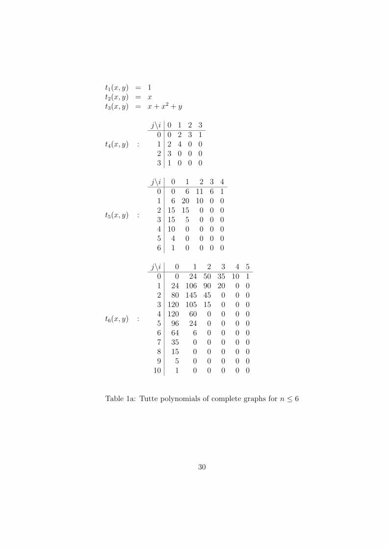
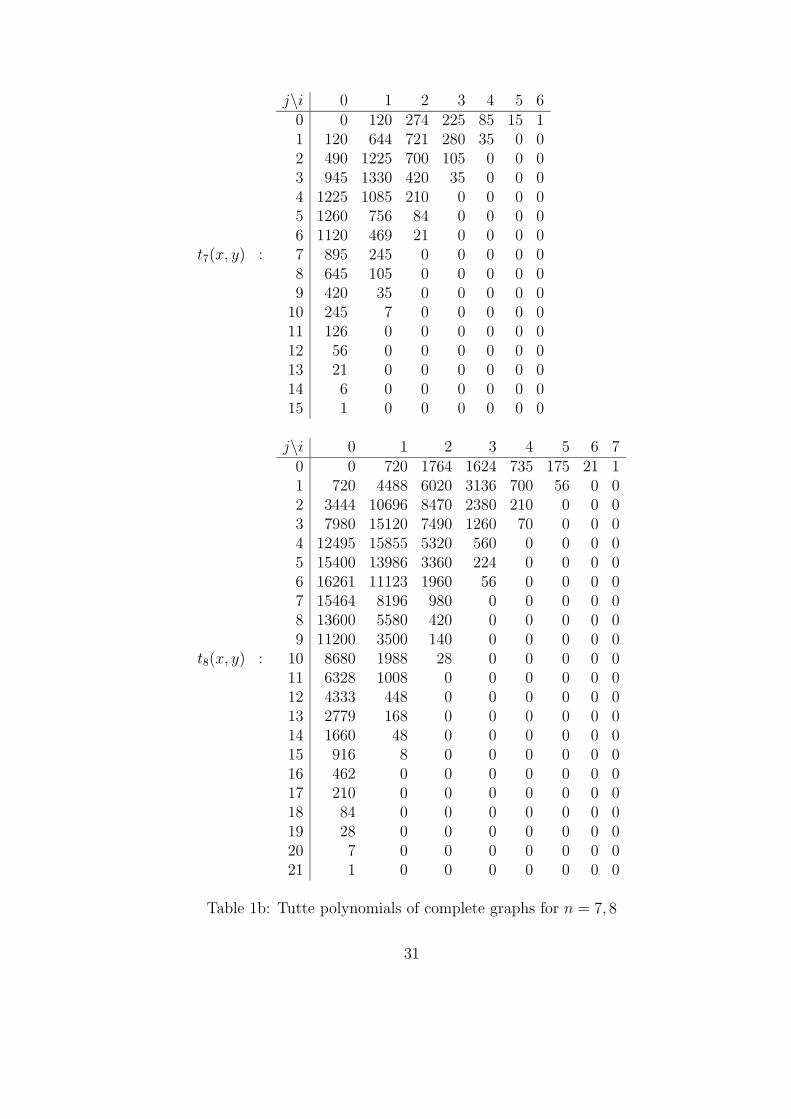
We will now give tables for various quantities that we have studied.Tables 1a and 1b contain the Tutte polynomials of the complete graphs tn(x, y)

for n ≤ 8. For n ≤ 3, the polynomials are written in the usual format. For4 ≤ n ≤ 8, we let

tn(x, y) =∑i,j

tn,i,jxiyj

and then display the coefficients in a rectangular matrix with the entry in row jand column i of the nth array being being tn,i,j.

Table 2 gives the specializations tn(y) = tn(1, y) which are also inversion enu-merators for trees.

29

t1(x, y) = 1t2(x, y) = xt3(x, y) = x+ x2 + y

t4(x, y) :

j\i 0 1 2 30 0 2 3 11 2 4 0 02 3 0 0 03 1 0 0 0

t5(x, y) :

j\i 0 1 2 3 40 0 6 11 6 11 6 20 10 0 02 15 15 0 0 03 15 5 0 0 04 10 0 0 0 05 4 0 0 0 06 1 0 0 0 0

t6(x, y) :

j\i 0 1 2 3 4 50 0 24 50 35 10 11 24 106 90 20 0 02 80 145 45 0 0 03 120 105 15 0 0 04 120 60 0 0 0 05 96 24 0 0 0 06 64 6 0 0 0 07 35 0 0 0 0 08 15 0 0 0 0 09 5 0 0 0 0 0

10 1 0 0 0 0 0

Table 1a: Tutte polynomials of complete graphs for n ≤ 6

30

t7(x, y) :

j\i 0 1 2 3 4 5 60 0 120 274 225 85 15 11 120 644 721 280 35 0 02 490 1225 700 105 0 0 03 945 1330 420 35 0 0 04 1225 1085 210 0 0 0 05 1260 756 84 0 0 0 06 1120 469 21 0 0 0 07 895 245 0 0 0 0 08 645 105 0 0 0 0 09 420 35 0 0 0 0 0

10 245 7 0 0 0 0 011 126 0 0 0 0 0 012 56 0 0 0 0 0 013 21 0 0 0 0 0 014 6 0 0 0 0 0 015 1 0 0 0 0 0 0

t8(x, y) :

j\i 0 1 2 3 4 5 6 70 0 720 1764 1624 735 175 21 11 720 4488 6020 3136 700 56 0 02 3444 10696 8470 2380 210 0 0 03 7980 15120 7490 1260 70 0 0 04 12495 15855 5320 560 0 0 0 05 15400 13986 3360 224 0 0 0 06 16261 11123 1960 56 0 0 0 07 15464 8196 980 0 0 0 0 08 13600 5580 420 0 0 0 0 09 11200 3500 140 0 0 0 0 0

10 8680 1988 28 0 0 0 0 011 6328 1008 0 0 0 0 0 012 4333 448 0 0 0 0 0 013 2779 168 0 0 0 0 0 014 1660 48 0 0 0 0 0 015 916 8 0 0 0 0 0 016 462 0 0 0 0 0 0 017 210 0 0 0 0 0 0 018 84 0 0 0 0 0 0 019 28 0 0 0 0 0 0 020 7 0 0 0 0 0 0 021 1 0 0 0 0 0 0 0

Table 1b: Tutte polynomials of complete graphs for n = 7, 8

31

t1(y) = 1

t2(y) = 1

t3(y) = 2 + y

t4(y) = 6 + 6 y + 3 y2 + y3

t5(y) = 24 + 36 y + 30 y2 + 20 y3 + 10 y4 + 4 y5 + y6

t6(y) = 120 + 240 y + 270 y2 + 240 y3 + 180 y4 + 120 y5 + 70 y6 + 35 y7

+15 y8 + 5 y9 + y10

t7(y) = 720 + 1800 y + 2520 y2 + 2730 y3 + 2520 y4 + 2100 y5 + 1610 y6 + 1140 y7

+750 y8 + 455 y9 + 252 y10 + 126 y11 + 56 y12 + 21 y13 + 6 y14 + y15

t8(y) = 5040 + 15120 y + 25200 y2 + 31920 y3 + 34230 y4 + 32970 y5 + 29400 y6

+24640 y7 + 19600 y8 + 14840 y9 + 10696 y10 + 7336 y11 + 4781 y12

+2947 y13 + 1708 y14 + 924 y15 + 462 y16 + 210 y17 + 84 y18 + 28 y19

+7 y20 + y21

Table 2: The inversion enumerator for trees

32

References

[1] G. E. Andrews, Catalan numbers, q-Catalan numbers and hypergeometricseries, J. Combin. Theory Ser. A, 44 (1987), 267–273.

[2] R. A. Bari, Chromatic polynomials and the internal and external activities ofTutte, in “Graph Theory and Related Topics (Proc. Int. Conf. Graph TheoryComb., University of Waterloo, 1977),” A. Bondy and U. S. R. Murty, eds.,Academic Press, New York (1979), 41–52.

[3] J. S. Beissinger, On external activity and inversions in trees, J. Combin. The-ory Ser. B 33 (1982), 87–92.

[4] A. Bjorner, The homology and shellability of matroids and geometric lattices,Chapter 7 in “Matroid Applications,” N. White ed., Cambridge UniversityPress, Cambridge, 1991, 226–283.

[5] T. Brylawski, The Tutte polynomial I: General theory, in “Matroid Theoryand its Applications (Proc. C. I. M. E., Varenna, 1980),” Naples (1982), 125–276.

[6] T. Brylawski and J. Oxley, The Tutte polynomial and its applications, Chap-ter 6 in “Matroid Applications,” N. White ed., Cambridge University Press,Cambridge, 1991, 123–225.

[7] W. F. Clocksin and C. S. Mellish, “Programming in Prolog,” Springer-Verlag,Berlin, 1981.

[8] H. H. Crapo, The Tutte polynomial, Aequationes Math. 3 (1969), 211–229.

[9] J. E. Dawson, A construction for a family of sets and its application to ma-troids, in “Combinatorial Mathematics VIII,” K. L. McAvaney ed., LectureNotes in Math., Vol. 884, Springer-Verlag, New York, NY, 1981, 136–147.

[10] J. E. Dawson, A collection of sets related to the Tutte polynomial of a matroid,in “Graph Theory Singapore 1983,” K. M. Koh and H. P. Yap eds., LectureNotes in Math., Vol. 1073, Springer-Verlag, New York, NY, 1984, 193–204.

[11] P. Doubilet, G.-C. Rota and R. P. Stanley, On the foundations of combinato-rial theory VI: The idea of generating function, in “Sixth Berkeley Symposiumon Mathematical Statistics and Probability,” (1972), 267–318.

33

[12] D. Foata, “La Serie Generatrice Exponentielle dans les Problemes d’Enumera-tion,” Seminaire de Mathematique Superieurs, No. 54, Presses de l’Universitede Montreal, Montreal, 1974

[13] D. Foata and J. Riordan, Mappings of acyclic and parking functions, Aequa-tiones Math. 10 (1974), 10–22.

[14] J. Furlinger and J. Hofbauer, q-Catalan numbers, J. Combin. Theory Ser. A,40 (1985), 248–264.

[15] A. M. Garsia and D. Stanton, Group actions on Stanley-Reisner rings andinvariants of permutation groups, Adv. in Math. 51 (1984), 107–201.

[16] I. M. Gessel, A noncommutative generalization and q-analog of the Lagrangeinversion formula, Trans. Amer. Math. Soc., 257 (1980), 455–482.

[17] I. M. Gessel, Enumerative applications of a decomposition for graphs anddigraphs, Discrete Math., to appear.

[18] I. M. Gessel and D.-L. Wang, Depth-first search as a combinatorial correspon-dence, J. Combin. Theory Ser. A, 26 (1979), 308–313.

[19] I. M. Gessel, B. E. Sagan and Y.-N. Yeh, Enumeration trees by inversions, J.Graph Theory, to be published.

[20] G. Gordon and L. Traldi, Generalized activities and the Tutte polynomial,Discrete Math. 85 (1990), 167–176.

[21] C. Greene and T. Zaslavsky, On the interpretation Whitney numbers throughthe arrangements of hyperplanes, zonotopes, non-Radon partitions, and ori-entations of graphs, Trans. Amer. Math. Soc., 280 (1983), 97–126.

[22] M. Haiman, Conjectures on the quotient ring of diagonal invariants, J. Alge-braic Combin., 3 (1994), 17–76.

[23] D. J. Kleitman and K. J. Winston, Forests and score vectors, Combinatorica1 (1981), 49–54.

[24] D. E. Knuth, “The Art of Computer Programming, Vol. 3: Sorting and Search-ing,” 1973; Addison-Wesley, Reading, MA.

[25] D. E. Knuth, Computer science and its relation to mathematics, Amer. Math.Monthly 81 (1974), 323–342.

34

[26] A. G. Konheim and B. Weiss, An occupancy discipline and applications, SIAMJ. Appl. Math. 14 (1966), 1266–1274.

[27] C. Krattenthaler, Counting lattice paths with linear boundary II, Osterreich.Akad. Wiss. Math.-Natur. Kl. Sitzungsber. II, 198 (1989), 171–199.

[28] G. Kreweras, Une famille de polynomes ayant plusieurs proprietes enumera-tives, Period. Math. Hungar., 11 (1980), 309–320.

[29] V. A. Liskovets, On the number of maximal vertices of a random acyclicdigraph, Theory Probab. Appl. 20 (1975) 401–409.

[30] C. L. Mallows and J. Riordan, The inversion enumerator for labeled trees,Bull. Amer. Math. Soc., 74 (1968), 92–94.

[31] P. Moszkowski, Arbres et suites majeures, Period. Math. Hungar. 20 (2)(1989), 147–154.

[32] A. Renyi, On connected graphs I, Publ. Math. Inst. Hungar. Acad. Sci., 4(1959), 385–388.

[33] J. Riordan, “Combinatorial Identities,” Wiley, New York, NY, 1968.

[34] J. Riordan, Ballots and trees, J. Combin. Theory 6 (1969), 408–411.

[35] R. W. Robinson, Counting labeled acyclic digraphs, in “New Directions in theTheory of Graphs,” F. Harary, ed., Academic Press, New York, 1973.

[36] V. I. Rodionov, On the number of labeled acyclic graphs, Discrete Math. 105(1992), 319–321.

[37] M. P. Schutzenberger, On an enumeration problem, J. Combin. Theory 4(1968), 219–221.

[38] R. P. Stanley, Acyclic orientations of graphs, Discrete Math., 5 (1973), 171–178.

[39] R. P. Stanley, Exponential structures, Studies Appl. Math., 59 (1978), 73–82.

[40] W. T. Tutte, A contribution to the theory chromatic polynomials, Canad. J.Math. 6 (1953), 80–91.

[41] W. T. Tutte, On dichromatic polynomials, J. Combin. Theory 2 (1967), 301–320.

35

[42] H. S. Wilf, “Generatingfunctionology,” Academic Press, Boston, MA, 1990.

[43] E. M. Wright, The number of connected sparsely edged graphs, J. GraphTheory, 1 (1977), 317–330.

36