Federal Reserve Bank of MinneapolisResearch Department

The Transition to a New EconomyAfter the Second Industrial Revolution∗

Andrew Atkeson and Patrick J. Kehoe

Working Paper 606

Revised July 2001

ABSTRACT

During the Second Industrial Revolution, 1860—1900, many new technologies, including electricity,were invented. These inventions launched a transition to a new economy, a period of about 70 yearsof ongoing, rapid technical change. After this revolution began, however, several decades passedbefore measured productivity growth increased. This delay is paradoxical from the point of viewof the standard growth model. Historians hypothesize that this delay was due to the slow diffusionof new technologies among manufacturing plants together with the ongoing learning in plants afterthe new technologies had been adopted. The slow diffusion is thought to be due to manufacturers’reluctance to abandon their accumulated expertise with old technologies, which were embodied inthe design of existing plants. Motivated by these hypotheses, we build a quantitative model oftechnology diffusion which we use to study this transition to a new economy. We show that itimplies both slow diffusion and a delay in growth similar to that in the data.

∗Atkeson and Kehoe thank the National Science Foundation. The views expressed herein are those of theauthors and not necessarily those of the Federal Reserve Bank of Minneapolis or the Federal Reserve System.

The period 1860—1900 is often called the Second Industrial Revolution because a large

number of new technologies were invented at that time. These inventions heralded a period

of about 70 years of ongoing, rapid technical change. Several decades passed, however, before

this revolution led to a new economy characterized by faster growth in productivity, measured

by output per hour.

In the standard growth model no such delay occur. Because technology is disembodied,

faster technical change results immediately in faster growth of measured productivity. Indeed,

David (1990) refers to this delay as a productivity paradox. He and other historians have

offered several hypotheses for this delay. Here we build a quantitative model of technology

diffusion that captures the main elements of these historians hypotheses. We show that this

model can generate a delay of several decades before a sustained increase in the pace of

technical change produces a new economy and we use the model to isolate the elements of

the historians hypotheses that are essential to generate such a delay.

Historians such as Schurr et al. (1960), Rosenberg (1976), Devine (1983), and David

(1990, 1991) focus on the development of electricity in the Second Industrial Revolution as

the driving force of the prolonged period of rapid technical change after this revolution. These

historians hypothesize that the development of electricity did not have an immediate payoff

in terms of higher productivity growth for two reasons. One is that new technologies based

on electricity diffused only slowly among U.S. manufacturing plants. The other is that, even

after a new plant embodying a new technology was built, learning how best to take advantage

of the technology took time.

At least two factors help account for the slow diffusion of electricity. As Devine (1983)

and David (1990, 1991) explain, manufacturing plants needed to be completely redesigned in

order to make good use of electric power. Indeed, David and Wright (1999, p. 4) argue that

“the slow pace of adoption prior to the 1920s was largely attributable to the unprofitability of

replacing still serviceable manufacturing plants embodying production technologies adapted

to the old regime of mechanical power derived from water and steam.” Rosenberg (1976)

argues that ongoing technical change itself helps account for the slow diffusion: people antic-

ipated ongoing improvements in technology and thus chose to wait for further improvements

before adopting the current frontier technology.

Several historians emphasize that learning how best to use the new technologies result-

ing from the Second Industrial Revolution took quite some time. Schurr et al. (1960, 1990)

discuss the process of learning following new applications of electricity to plant and machine

design. They argue that the benefits of adopting electricity went far beyond the direct cost

savings from reduced energy consumption. The electrification of plants opened opportuni-

ties for continual innovation in processes and procedures within an existing plant to improve

overall productive efficiency. In practice, managers needed time to learn how best to take

advantage of these opportunities. Chandler (1992) emphasizes that the knowledge gained

in using new technologies was mostly organization-specific and, hence, difficult to transfer

across organizations.

Our model of technology diffusion attempts to capture the main elements of these

historians’ hypotheses. The idea of Devine (1983) and David (1991) that manufacturers

needed to build new plants in order to adopt the new technologies based on electricity is

built into the model by having new technologies embodied in the design of new manufacturing

plants.

The ongoing technical change discussed by Rosenberg (1976) is modeled as ongoing

2

improvements in the technology embedded in these plant designs. The process of learning

within an existing plant, discussed by Schurr et al. (1990) and Chandler (1992), is modeled

as a stochastic process for the productivity with which that plant is able to implement the

technology embodied in its design. Thus, in the model, the decision to adopt new technology

amounts to a decision to close existing manufacturing plants based on old technologies and

replace them with new plants based on the current frontier technology and then to undergo

the process of learning to use that technology.

We quantify our model to capture the main patterns of industry evolution at the plant

level in the U.S. economy. In the model, as in the data, the process of starting a new plant is

turbulent and time-consuming. New plants tend to start small in terms of both employment

and output and to fail often. Surviving plants tend to grow for as long as 20 years. We

model this evolution as resulting from a stochastic process for plant-specific productivity

(as in Hopenhayn and Rogerson 1993). We quantify this process by observing that the size

of plants is determined by their specific productivities. We choose the parameters of this

stochastic process to replicate the patterns of birth, growth, and death of plants in the U.S.

economy as documented by Davis, Haltiwanger, and Schuh (1996).

We then ask what our model predicts about the transition from an old economy with

a relatively slow pace of technical change to a new one with a relatively fast pace. In order

to capture the notion that this transition began with the Second Industrial Revolution, we

model the transition as arising from a once-and-for-all increase, starting in 1869, in the rate

of improvement in the frontier technology embodied in the design of new plants. During the

transition, new technologies diffuse only slowly, plants learn to use them efficiently over time,

and there is a several-decade-long delay before the growth in output per hour climbs to its

3

new steady-state level. In this transition, the path of diffusion of new technology in the model

is similar to the path of diffusion of electric power in U.S. manufacturing plants in the data

during 1869—1939. The trends in the growth of output per hour generated by the model are

also similar to those in the data for the period 1869—1969.

Two features of our model are critical in generating the slow transition. One is that,

in the old economy, manufacturers build up a larger stock of knowledge using their embodied

technologies than they do in the new economy. In the old economy, the pace of technical

change and the diffusion of new technologies is relatively slow, and thus manufacturers spend

a relatively long time building up knowledge and expertise with a given technology. At

the beginning of the transition, manufacturers are reluctant to abandon this large stock of

knowledge to adopt what, initially, is only a marginally superior technology. We demonstrate

the importance of this feature by showing that if the stock of knowledge is not larger in the old

economy than in the new one, the transition is almost immediate. The other model feature

critical for the slow transition is our assumption that new technologies are embodied in the

design of plants rather than disembodied. We show that if new technologies are disembodied,

as they are in the standard growth model, the transition is almost immediate.

One implication of our model is that the speed of diffusion of new technologies should

follow this pattern: slow in the old economy, medium during the transition, and fast in the

new economy. We argue that this implication is consistent with the data on the diffusion of

steam power in the old economy, electricity in the transition, and a variety of technologies in

the new economy.

Our study is related to several strands of literature. The process of diffusion in our

model is closely related to that in the model of Chari and Hopenhayn (1991). In the Chari-

4

Hopenhayn model, workers build up knowledge capital that is specific to a certain technology.

and they lose this capital if they adopt a different technology. Chari and Hopenhayn (1991)

argue that their model has two important implications that most other models of diffusion

do not generate. First, when a new technology is introduced, workers do not simply abandon

built-up knowledge in old technologies and adopt the new one. Rather they adopt the new

technology only slowly. Second, investment in the old technologies continues even after a

new technology is introduced. Our model shares these implications, and they are critical for

generating our results.

Jovanovic and MacDonald (1994) develop a competitive model of diffusion of a single

innovation in an industry. Their model is more detailed than ours in that theirs considers

separate learning and production decisions and incorporates spillovers of knowledge from

one plant to another. However, their study is concerned with questions appropriate for a

partial equilibrium framework, while we are concerned with questions relevant for a general

equilibrium framework.

Many other studies are more generally related to ours. The process of industry evolu-

tion and learning at the plant level in our model is related to that in the models of Jovanovic

(1982), Hopenhayn and Rogerson (1993), and Campbell (1998). The role of learning in the

transition to a new economy is related to the role of learning in the theoretical models of

general purpose technologies of Aghion and Howitt (1998) and Helpman and Trajtenberg

(1998) and in the applied work on the post-1974 productivity slowdown by Hornstein and

Krusell (1996) and Greenwood and Yorukoglu (1997). The impact of an economy-wide tran-

sition on growth is related to that in some theories of the transition in Eastern European

countries after the collapse of communism (Atkeson and Kehoe 1993, Aghion and Blanchard

5

1994, Brixiova and Kiyotaki 1997, and Castanheira and Roland 2000).

1. Productivity and diffusion after theSecond Industrial Revolution

Many of the new technologies that had a profound impact on living standards in the

20th century were invented between 1860 and 1900. These technologies include electricity, the

internal combustion engine, petroleum and other chemicals, telephones and radios, and indoor

plumbing. (See Gordon 2000a for a description.) While all of these inventions undoubtedly

had a substantial economic impact, we follow Schurr et al. (1960, 1990), Rosenberg (1976),

Devine (1983), and David (1990, 1991) and focus on the new technologies based on electricity.

In this section, we document the gradual increase in the growth of productivity–

output per hour–in U.S. manufacturing over the period 1869—1969 and the gradual diffusion

of electric power in U.S. manufacturing over the period 1869—1939. (We choose these dates

because, early in the sample period, the data are derived from the U.S. Census Bureau’s

censuses of manufacturing establishments taken every decade starting in 1869.) We also

review the chronology of the development of the modern technology of electric power in

manufacturing.

In Figure 1, we plot output per hour in the U.S. manufacturing industry over the

period 1869—1969 using annual data from the U.S Department of Commerce (1973). We also

show linear trends for the three periods 1869—99, 1899—1929, and 1949—69. (These periods are

chosen to omit the Great Depression and World War II.) The trend growth rates of output

per hour in these three periods increased gradually, from 1.6% to 2.6% to 3.3%, respectively.

(Gordon 2000b documents a similar gradual acceleration for the growth of output per hour

for the economy as a whole.)

6

To document the slow diffusion of electricity, in Figure 2 we plot the fraction of me-

chanical power in U.S. manufacturing establishments that is derived from water, steam, and

electricity during 1869—1939. (See Devine 1983.) Before 1899, more than 95% of mechanical

power was derived from water and steam. Between 1899 and 1929, electricity use gradually

replaced water and steam, so that by 1929, over 75% of mechanical power was electric. If

we measure the diffusion of electricity starting in 1869, then we see that it took 50 years

for electricity to provide 50% of mechanical power. This measure of the speed of diffusion

is sensitive to the choice of starting date. An alternative measure of the speed of diffusion

commonly used in the literature is the time required for a technology to diffuse from 5% to

50% of its potential users. For electricity in U.S. manufacturing, this occurred over the 20

years from 1899 to 1919.

Our chronology of the development of electricity after the Second Industrial Revo-

lution follows that of Devine (1983) and David (1990, 1991). In the period 1869—99, the

modern technology of electricity generation and distribution and motors driven by electricity

was developed. Figure 3, taken from the work of Devine (1983), displays the gradual devel-

opment of the modern technology of electric power in manufacturing. Briefly, the two major

developments documented in this figure were the shift in the architecture of factories to take

advantage of electric motors (outlined in panel A) and the development of the technology of

producing electricity in large, centralized power plants and then shipping it over a distance

to factories (outlined in panel B). In the period 1899—1929, this modern technology gradually

diffused throughout the manufacturing sector. In the period 1929—69, this modern technology

was the dominant one in manufacturing.

7

2. Links Between Historical Analyses and the Model

Here we report on three features of the data discussed by historians that motivate

corresponding features in our model: (1) the change to electric power from steam and water

power led to major changes in factory design and machine organization that went hand in

hand with electrification; (2) the process of improving efficiency through changes in factory

design continued for decades, through at least the 1980s; and (3) for each new factory design,

the process of learning how best to use the new design took an extended period of time.

Our assumption that technology is embodied in plant design is motived by the analysis

of diffusion of Devine (1983) and David (1990, 1991). They argue that the adoption of the

modern technology of electricity required a complete redesign of the manufacturing plant. In

steam- and water-driven plants, power was distributed mechanically throughout the factory

by a series of shafts and belts called a direct-drive system. In modern electric plants, power

is distributed as electricity through wires to individual motors in what is called a unit-drive

system.

Devine (1983, pp. 350, 352) describes the direct-drive system used in steam- and

water-driven plants this way:

Until late in the nineteenth century, production machines were connected by a

direct mechanical link to the power sources that drove them. In most factories,

a single centrally located prime mover, such as a water wheel or steam engine,

turned iron or steel “line shafts” via pulleys and leather belts. These line shafts–

usually 3 inches in diameter–were suspended from the ceiling and extended the

entire length of each floor of a factory, sometimes even continuing outside to

8

deliver power to another building. Power was distributed between floors of large

plants by belts running through holes in the ceiling . . . . The line shafts turned,

via pulleys and belts, “countershafts”–shorter ceiling-mounted shafts parallel to

the line shafts. Production machinery was belted to the countershafts and was

arranged, of necessity, in rows parallel to the line shafts . . . . The entire network

of line shafts and countershafts rotated continuously–from the time the steam

engine was started up in the morning until it was shut down at night–no matter

how many machines were actually being used. If a line shaft or the steam engine

broke down, production ceased in a whole room of machines or even in the entire

factory until repairs were made.

Panel A of Figure 4 (from Devine 1983) illustrates this direct-drive system of power.

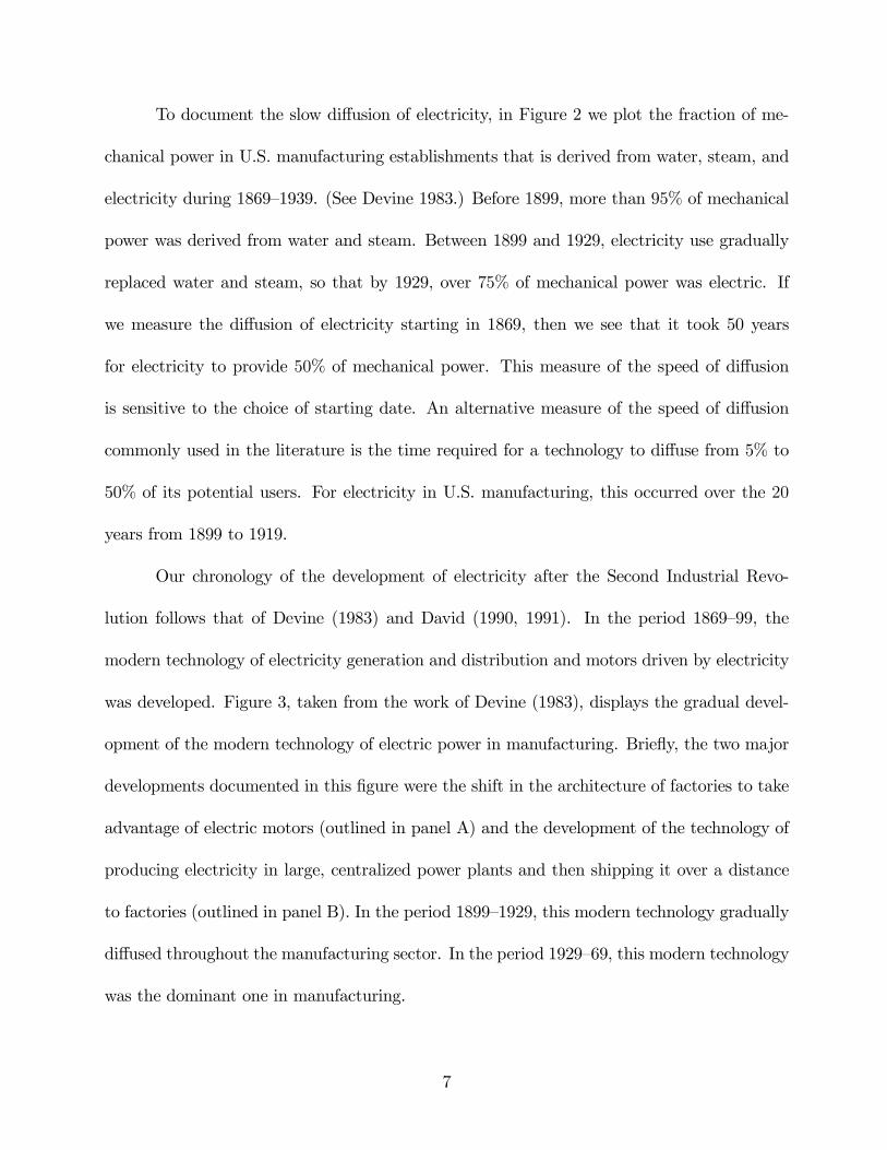
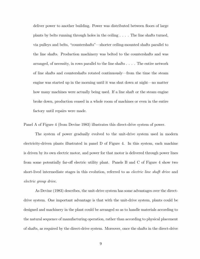
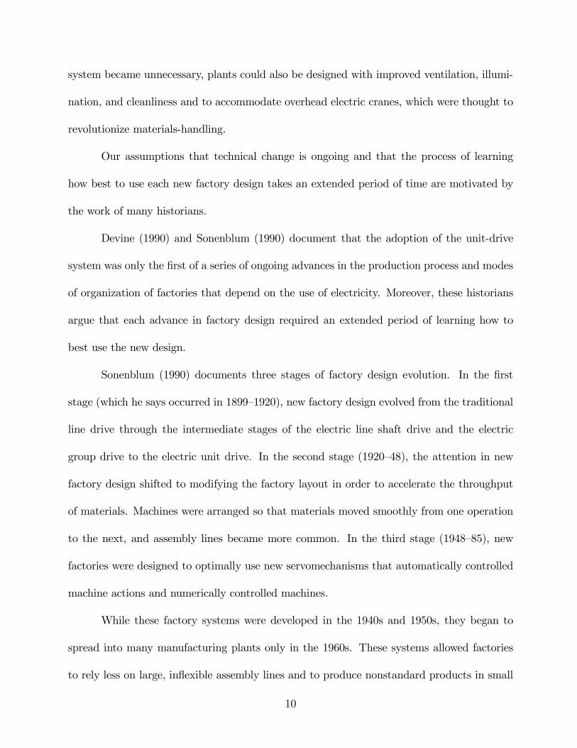
The system of power gradually evolved to the unit-drive system used in modern

electricity-driven plants illustrated in panel D of Figure 4. In this system, each machine

is driven by its own electric motor, and power for that motor is delivered through power lines

from some potentially far-off electric utility plant. Panels B and C of Figure 4 show two

short-lived intermediate stages in this evolution, referred to as electric line shaft drive and

electric group drive.

As Devine (1983) describes, the unit-drive system has some advantages over the direct-

drive system. One important advantage is that with the unit-drive system, plants could be

designed and machinery in the plant could be arranged so as to handle materials according to

the natural sequence of manufacturing operation, rather than according to physical placement

of shafts, as required by the direct-drive system. Moreover, once the shafts in the direct-drive

9

system became unnecessary, plants could also be designed with improved ventilation, illumi-

nation, and cleanliness and to accommodate overhead electric cranes, which were thought to

revolutionize materials-handling.

Our assumptions that technical change is ongoing and that the process of learning

how best to use each new factory design takes an extended period of time are motivated by

the work of many historians.

Devine (1990) and Sonenblum (1990) document that the adoption of the unit-drive

system was only the first of a series of ongoing advances in the production process and modes

of organization of factories that depend on the use of electricity. Moreover, these historians

argue that each advance in factory design required an extended period of learning how to

best use the new design.

Sonenblum (1990) documents three stages of factory design evolution. In the first

stage (which he says occurred in 1899—1920), new factory design evolved from the traditional

line drive through the intermediate stages of the electric line shaft drive and the electric

group drive to the electric unit drive. In the second stage (1920—48), the attention in new

factory design shifted to modifying the factory layout in order to accelerate the throughput

of materials. Machines were arranged so that materials moved smoothly from one operation

to the next, and assembly lines became more common. In the third stage (1948—85), new

factories were designed to optimally use new servomechanisms that automatically controlled

machine actions and numerically controlled machines.

While these factory systems were developed in the 1940s and 1950s, they began to

spread into many manufacturing plants only in the 1960s. These systems allowed factories

to rely less on large, inflexible assembly lines and to produce nonstandard products in small

10

batches. Moos (1957) and Slesinger (1958) also discuss the changes in plant design driven

by the development of automatically controlled machines and the learning required to take

advantage of such plants. As Devine (1990) discusses, in the 1980s the evolution of factory

design evolved to accommodate new methods of computer materials-handling and computer-

integrated manufacturing in which a computer controls whole groups of machines. Figure 5

(from Devine 1990) gives a brief chronology.

Chandler (1992, p. 84) discusses the type of built-up organizational capabilities that

resulted from firms learning to efficiently use the technologies developed in the Second Indus-

trial Revolution. He argues that the learned capabilities that resulted from solving problems

of scaling up the processes of production manifest themselves in firms’ production and distri-

bution facilities. These learned capabilities were developed through trial and error, feedback,

and evaluation and were organization-specific.

3. A Model of Technology Diffusion

In this section, we develop our quantitative model of technology diffusion. We build

into the model the three key elements detailed in the last section: (1) new technologies are

embodied in plants; (2) improvements in the technology for new plants are ongoing; and

(3) new plants must undergo an extended period of learning to use their technology most

efficiently.

Our model economy is as follows. Time is discrete and is denoted by periods t =

0, 1, 2, . . . . The economy has two types of agents: workers and managers. There exist a

continuum of size 1 of workers and a continuum of size 1 of managers.

Workers are each endowed with one unit of labor per period, which they supply in-

11

elastically. Workers are also endowed with the initial stock of physical capital and ownership

of the plants that exist in period 0. Workers have preferences over consumption given by

P∞t=0 β

t log(cwt), where β is the discount factor. Given sequences of wages and intertemporal

prices {wt, pt}∞t=0, initial capital holdings k0, and an initial value a0 of the plants that exist

in period 0, workers choose sequences of consumption {cwt}∞t=0 to maximize utility subject to

the budget constraint

∞Xt=0

ptcwt ≤∞Xt=0

ptwt + k0 + a0.(1)

Managers are endowed with one unit of managerial time in each period. Managers have

preferences over consumption given byP∞t=0 β

t log(cmt). Given sequences of managerial wages

and intertemporal prices {wmt, pt}∞t=0, managers choose consumption {cmt}∞t=0 to maximize

utility subject to the budget constraintP∞t=0 ptcmt ≤

P∞t=0 ptwmt. Notice that we have given

all the initial assets to the workers. Since worker and manager utilities are identical and

homothetic, aggregate variables do not depend on the initial allocation of assets.

Production in this economy is carried out in plants. In any period, a plant is char-

acterized by its specific productivity A and its age s. To operate, a plant uses one unit of

a manager’s time, physical capital, and (workers’) labor as variable inputs. If a plant with

specific productivity A operates with one manager, capital k, and labor l, the plant produces

output

y = zA1−νF (k, l)ν,(2)

where the function F is linearly homogeneous of degree 1 and the parameter ν ∈ (0, 1).

The technology parameter z is common to all plants and grows at an exogenous rate. We

12

call z economy-wide productivity. Following Lucas (1978, p. 511), we call ν the span of

control parameter of the plant’s manager. The parameter ν may be interpreted more broadly

as determining the degree of diminishing returns at the plant level. We refer to the pair

(A, s) as the plant’s organization-specific capital, or simply its organization capital. This pair

summarizes the built-up knowledge that distinguishes one organization from another.

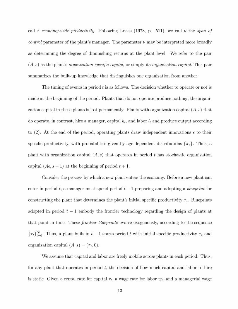
The timing of events in period t is as follows. The decision whether to operate or not is

made at the beginning of the period. Plants that do not operate produce nothing; the organi-

zation capital in these plants is lost permanently. Plants with organization capital (A, s) that

do operate, in contrast, hire a manager, capital kt, and labor lt and produce output according

to (2). At the end of the period, operating plants draw independent innovations ² to their

specific productivity, with probabilities given by age-dependent distributions {πs}. Thus, a

plant with organization capital (A, s) that operates in period t has stochastic organization

capital (A², s+ 1) at the beginning of period t+ 1.

Consider the process by which a new plant enters the economy. Before a new plant can

enter in period t, a manager must spend period t− 1 preparing and adopting a blueprint for

constructing the plant that determines the plant’s initial specific productivity τ t. Blueprints

adopted in period t − 1 embody the frontier technology regarding the design of plants at

that point in time. These frontier blueprints evolve exogenously, according to the sequence

{τ t}∞t=0. Thus, a plant built in t − 1 starts period t with initial specific productivity τ t and

organization capital (A, s) = (τ t, 0).

We assume that capital and labor are freely mobile across plants in each period. Thus,

for any plant that operates in period t, the decision of how much capital and labor to hire

is static. Given a rental rate for capital rt, a wage rate for labor wt, and a managerial wage

13

wmt, the operating plant chooses employment of capital and labor to maximize static returns:

maxk,lztA

1−νF (k, l)ν − rtk − wtl − wmt.(3)

The static returns to the owner of a plant with organization capital (A, s) in t are given by

dt(A)− wmt, where dt(A) = ztA1−νF(kt(A), lt(A))ν − rtkt(A)− wtlt(A) and kt(A) and lt(A)

are the solutions to this problem.

The decision whether or not to operate a plant is dynamic. This decision problem is

described by the Bellman equation

Vt(A, s) = max [0, Vct (A, s)](4)

V ct (A, s) = dt(A)− wmt +pt+1pt

Z²Vt+1(A², s+ 1)πs+1(d²),

where the sequences {τ t, wt, rt, wmt, pt}∞t=0 are given. The value Vt(A, s) is the expected

discounted stream of returns to the owner of a plant with organization capital (A, s). This

value is the maximum of the returns from closing the plant and those from operating it. The

term V ct (A, s), the expected discounted value of operating a plant of type (A, s), consists of

current returns dt(A) − wmt and the discounted value of expected future returns Vt+1(A, s).

The plant operates only if the expected returns V ct (A, s) from operating it are nonnegative.

The decision whether or not to hire a manager to prepare a blueprint for a new plant

is also dynamic. In period t, this decision is determined by the equation

V 0t = −wmt +pt+1ptVt+1(τ t+1, 0).(5)

The value V 0t is the expected stream of returns to the owner of a new plant, net of the cost

wmt of paying a manager to prepare the blueprint for the plant. Such blueprints are prepared

only if the expected returns from these plans, V 0t , are nonnegative.

14

Let µt denote the distribution in period t of organization capital across plants that

might operate in that period, where µt(A, s) is the measure of plants of age s with productivity

less than or equal to A. Let φt ≥ 0 denote the measure of managers preparing blueprints for

new plants in t. Denote the measure of plants that operate in t by λt(A, s). This measure is

determined by µt and the sign of the function Vct (A, s) according to

λt(A, s) =Z A

01V c(a, s)µt(da, s),

where 1V c(a, s) = 1 if V ct (a, s) ≥ 0 and 0 otherwise. For each plant that operates, an

innovation to its specific productivity is drawn, and the distribution µt+1 is determined from

λt,φt, {πs} , and {τ t} as follows:

µt+1(A0, s+ 1) =

ZAπs+1(A

0/A)λt(dA, s)(6)

for s ≥ 0 and µt+1(τ t+1, 0) = φt.

Let kt denote the aggregate physical capital stock. Then the resource constraints for

physical capital and labor arePs

RA kt(A)λt(dA, s) = kt and

Ps

RA lt(A)λt(dA, s) = 1. The

resource constraint for aggregate output is cwt+cmt+kt+1 = yt+(1−δ)kt, where yt is defined

by yt = ztPs

RAA

1−νF(kt(A), lt(A))νλt(dA, s). The resource constraint for managers is

φt +Xs

ZAλt(dA, s) = 1.(7)

Managers are hired to prepare blueprints for new plants only if V 0t ≥ 0. Since there

is free entry into the business of starting new plants, in equilibrium we require V 0t ≤ 0. We

summarize this condition as V 0t φt = 0. Also, in equilibrium, a0 =Ps

RA V0(A, s)µ0(dA, s) is

the value of the workers’ initial assets.

15

Given a sequence of frontier blueprints and economy-wide productivities {τ t, zt}, initial

endowments k0 and a0, and an initial measure µ0, an equilibrium in this economy is a collection

of sequences of consumption; aggregate capital {cmt, cwt, kt} ; allocations of capital and labor

across plants {kt(A), lt(A)}; measures of operating plants, potentially operating plants, and

managers preparing plans for plantsnλt, µt+1,φt

o; value functions and operating decisions

{dt, Vt,V ct , V 0t }; and prices {wt, rt, wmt, pt, }, all of which satisfy the above conditions.

To get a sense of the process for the birth, growth, and death of plants which our model

generates, consider Figure 6. In this figure we show the evolution of the specific productivity

of two plants that both enter in 1860. Both of these plants start with productivity equal to

that of the frontier blueprint in 1860, namely, τ1860. This frontier blueprint grows exogenously

over time at a constant rate as shown by the straight line labeled log τ t. These plants each

experience random shocks to their plant-specific productivity drawn from distributions πs

with age-dependent means denoted by πs. Plant 1 is relatively lucky in that it draws especially

favorable shocks to its specific productivity, while plant 2 is relatively unlucky.

In every period, each plant makes a decision whether to continue or to exit. This

decision is based on a comparison of the plant’s current specific productivity and its future

prospects for learning determined by πs relative to the alternative of exiting and starting a

new plant with the current frontier blueprint. Plant 1 has relatively high specific productivity;

hence, it exits only after 30 years. In contrast, plant 2 has relatively low specific productivity;

hence, it exits much sooner. After each of these plants exits, the manager in the plant starts

a new plant with the current frontier blueprint and begins the process of building up specific

productivity in the new plant.

In our model, new technologies diffuse as new plants embodying these technologies

16

are born and grow. Figure 6 also illustrates the mechanics of this diffusion. In 1863, the

manager of plant 2 decides to exit and start a new plant that embodies the frontier blueprint

of 1864 and then begins to learn with that new technology. Likewise, in 1890 the manager of

plant 1 decides to exit and start a new plant that embodies the frontier blueprint of 1891 and

then begins to learn with that new technology. In this manner, new technologies gradually

replace old ones. Since our model has many such plants, each with different shocks to specific

productivity, this diffusion of new technologies occurs smoothly over time.

4. Linking Specific Productivity and Size

Now we link the level of specific productivity of a plant or a cohort of plants to the

size of these units. We use this link to argue that the data imply that the aggregate specific

productivity of a cohort of plants of a given age grows substantially as the cohort ages. We

then show that the model can be rewritten with size instead of specific productivity as a state

variable. This alternative representation is convenient when we quantify the model.

We start with the data on employment by plants of different ages. Figure 7 presents

the share of manufacturing employment in plants of various age groups stated as the share

of workers employed by a one-year cohort within each age group as of 1988.1 In the figure,

we see that as a cohort of plants ages from newborn to 20 years old, it employs a growing

share of the labor force; after that, its share declines. In our model, these data imply that

the aggregate of specific productivities across a cohort of plants is also growing faster than

the aggregate of all plants for the plants’ first 20 years.

We develop the relationship between the employment share and the aggregate specific

productivity of a cohort of plants by first deriving the relationship between the size and the

17

specific productivity of a single plant and then aggregating across plants in the cohort. To

that end, consider the allocation of capital and labor across plants at any point in time.

Since capital and labor are freely mobile across plants, the problem of allocating these factors

across plants in period t is static. For a given distribution λt of organization capital, it is

convenient to define

nt(A) =A

At(8)

as the size of a plant of type (A, s) in period t, where

At =Xs

ZAAλt(dA, s)(9)

is the aggregate of the specific productivities across all plants. The variable nt(A) measures

the size of the plant in terms of its capital or labor or output, in that the equilibrium

allocations are

kt(A) = nt(A)kt, lt(A) = nt(A)lt, and yt(A) = nt(A)yt,(10)

where yt = ztA1−νt F (kt, lt)ν is aggregate output. To see this, note that since the production

function F is linear-homogeneous of degree 1 and there is only one fixed factor, all oper-

ating plants in this economy use physical capital and labor in the same proportions. The

proportions are those that satisfy the resource constraints for capital and labor.

Now define the aggregate of the specific productivities of a cohort of plants of age s

as At,s =RAAλt(dA, s)/At. Note from (8) that At,s =

RA nt(A)λt(dA, s). Using (10), we then

have this

Proposition 1. The aggregate of specific productivities in plants of age s relative to that in

18

all plants is the share of total employment in those plants, that is, At,s = lt,s, where

lt,s =ZA

lt(A)

ltλt(dA, s).(11)

Note for later that we use this proposition in our data analysis when we identify lt,s with the

employment shares in Figure 7 and use those shares to back out the relative productivities

of cohorts of plants of different ages.

We now show that on a balanced growth path, for each plant we can replace the state

variable specific productivity A with the state variable size n. To ensure that our model has a

balanced growth path, we assume that F (k, l) has the Cobb-Douglas form kθl1−θ. We define

a balanced growth path in this economy as an equilibrium in which the following conditions

hold: The quality of the frontier blueprint τ t and the productivity At grow at a constant rate

1 + gτ , the economy-wide level of technology zt grows at a constant rate 1 + gz, aggregate

variables yt, ct, kt, wt, and wmt grow at a rate 1+g, where 1+g = [(1+gz)(1+gτ )1−ν]1/(1−νθ);

variables φt, V0t , and rt are constant; the distributions of organization capital across plants

satisfy µt+1(A, s) = µt(A/(1 + gτ ), s) and λt+1(A, s) = λt(A/(1 + gτ ), s) for all t, A, s; and

Vt+1(A, s) = (1 + g)Vt(A/(1 + gτ ), s), dt+1(A, s) = (1 + g)dt(A/(1 + gτ ), s), and V ct+1(A, s) =

(1 + g)V ct (A/(1 + gτ ), s) for all t, A, s.

Along the balanced growth path, we can recast our state variables as (n, s) instead of

(A, s) as follows. Define the function W (n, s) = V0(A, s)/y0(1− ν), where n = A/A0. Define

the function W c(n, s) from V c0 (A, s) in a similar way. Let ωm = wm0/y0(1− ν) and {ρs} be

the cumulative distribution functions of η = ²/(1 + gτ )(1 + gz) induced by {πs} . We refer to

{ρs} as the steady-state distributions of shocks to plant size. Consider the another Bellman

19

equation

W (n, s) = max [0,W c(n, s)](12)

W c(n, s) = n− ωm + βZηW (nη, s+ 1)ρs+1(dη),

where ωm = βW (τ 0/A0, 0). Since the value functions Vt and V ct solve the original Bellman

equation (4) along the steady-state path, the functions W and W c defined above satisfy

this second Bellman equation. The terms in (12) have the same interpretation as those in

(4) as descriptions of the returns to operating or closing a plant of size n and age s. The

function W c(n, s) defines an operating rule: plants with W c(n, s) ≥ 0 operate, and those

with W c(n, s) < 0 do not.

We use microeconomic data to quantify the shocks to plant size η. Note that since

only the product (1 + gτ )(1 + gz) enters the definition of shocks to size η, the data on the

size-age distribution of plants do not pin down the relative contribution to growth in the

Solow residual of growth in the two types of technology: frontier and economy-wide.

5. Two Model Implications

Now we discuss what the model implies for two key concepts: the average productivity

of plants and the diffusion of new technologies among them.

A. For Average Productivity at the Plant Level

We argue that the data support the view that plants accumulate a large amount of

organization-specific capital as they age. This capital is reflected in their size and not in some

measure of their average productivity. That plants grow in size with age is clear from the data

on the employment shares of plants of different ages presented by Davis, Haltiwanger, and

20

Schuh (1996) (at least for plants’ first 20 years of production) as well as from the panel data of

Jensen, McGuckin, and Stiroh (2001). That these differences in organization-specific capital

are not reflected in average productivity of capital or labor is documented by Bartelsman and

Dhrymes (1998) and Jensen, McGuckin, and Stiroh (2001).

Bartelsman and Dhrymes (1998) study a sample of manufacturing plants drawn from

the U.S. Census Bureau’s Longitudinal Research Database (LRD). For this sample, they

report a geometric weighted-average of capital and labor productivity

µyitkit

¶α µyitlit

¶1−α

by age category and size decile as measured by the average size of employment over the period

1972—86, where the weights are obtained from a regression of outputs on inputs. We report

their values for this measure by age categories and size deciles in Figures 8A and 8B. While

Bartelsman and Dhrymes (1998) find variations in this measure across individual plants,

Figures 8A and 8B show that there is no systematic relationship between their measure of

average productivity and either age or size.

Jensen, McGuckin, and Stiroh (2001) study labor productivity measured as value

added per hour worked in a more extensive sample of manufacturing plants drawn from the

LRD. They note that labor productivity varies extensively across individual plants. When

they average productivity across plants in a cohort, however, they find no systematic rela-

tionship between labor productivity and age. Indeed, Jensen, McGuckin, and Stiroh report

that after about 5—10 years, all cohorts of surviving plants have similar productivity levels.

This feature of the data distinguishes our approach for measuring the specific pro-

ductivity of plants from much of the literature on learning-by-doing. The early literature

21

on learning-by-doing studies individuals performing specific tasks or groups of individuals

performing a given number of tasks. (See the survey in Argote and Epple 1990.) This early

literature shows that for a wide variety of tasks, an individual’s average productivity increases

with the number of times the task is performed. Based on this literature, one might think

that the extent of learning in plants might show up as changes in the average productivity

of labor in plants over time. As we show below, however, in our model, even though there is

differential learning across plants, in each period the average productivity of labor is constant

across plants. We have argued that this implication of our model is consistent with the data.

An individual who learns shows increases in labor productivity. An organization that

learns grows by adding variable factors so as to keep labor productivity constant (at least

with Cobb-Douglas production). Hence, the key variable to look at to determine the amount

of organization-specific capital in a plant is not some measure of either its labor productivity

or its capital productivity, but rather some measure of relative size.

To see this, consider a simplified version of our model in which the output in plant

number i in period t is given by

yit = ztA1−νit lνit,(13)

where Ait may depend on the age of the plant. In equilibrium, each plant in each period t

chooses labor lit to maximize profits, which implies that

lit = AitltAt,(14)

where lt =Pi lit and At =

PiAit. Hence, taking logs of (13) and substituting for Ait from

(14) gives that, in equilibrium, labor productivity is given by

yitlit= zt(At/lt)

1−ν

22

and, hence, is constant across all plants regardless of their specific productivity Ait. If

we extend the model to include capital, then (10) implies that yt(A)/lt(A) = yt/lt and

yt(A)/kt(A) = yt/kt. Hence, our model predicts that both of these measures of average

productivity are constant across plants.

B. For Diffusion

We use our model to study the diffusion of technologies that are embodied in the design

of manufacturing plants. In this section, we define our measure of diffusion and discuss how

we compare the implications of the model to data on diffusion.

Formally, we measure the diffusion of new technologies in our model as follows. Let

yt,s =ZA

yt(A)

ytλt(dA, s)

denote the fraction of total output yt produced in plants of age s. We measure the diffusion

in period t+ k of technologies developed in period t or later by

Dt,t+k =kXs=0

yt,s,(15)

which is the fraction of output produced in plants using these technologies. In our model,

this diffusion is also equal to the fraction of labor employed in plants using these technologies,

so that Dt,t+k =Pks=0 lt,s. With this link between diffusion and employment shares by age,

we can use our model and the data from Figure 7 to measure the implied diffusion rate of

new embodied technologies in recent years.

In Figure 9 we plot the diffusion of new embodied technologies Dt,t+k implied by our

model in the steady state as a function of the age of the technology k. Since our data on the

employment shares of plants cover plants only up to age 25, we show diffusion only up to this

23

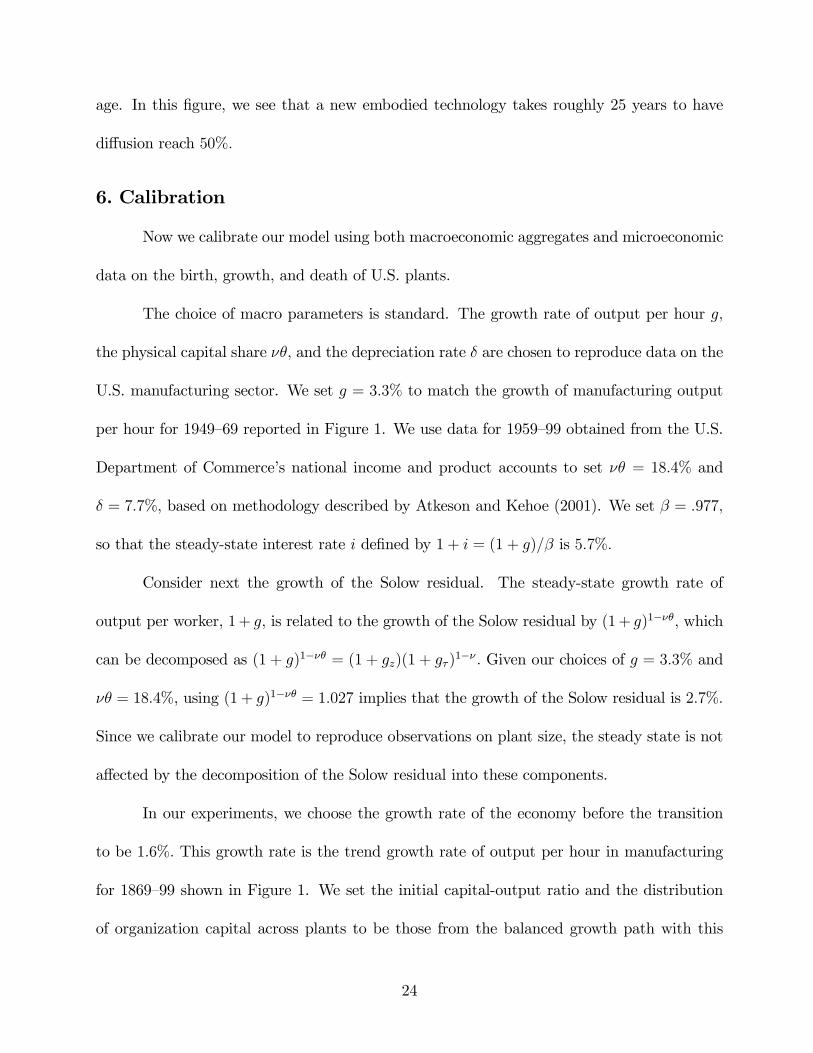
age. In this figure, we see that a new embodied technology takes roughly 25 years to have

diffusion reach 50%.

6. Calibration

Now we calibrate our model using both macroeconomic aggregates and microeconomic

data on the birth, growth, and death of U.S. plants.

The choice of macro parameters is standard. The growth rate of output per hour g,

the physical capital share νθ, and the depreciation rate δ are chosen to reproduce data on the

U.S. manufacturing sector. We set g = 3.3% to match the growth of manufacturing output

per hour for 1949—69 reported in Figure 1. We use data for 1959—99 obtained from the U.S.

Department of Commerce’s national income and product accounts to set νθ = 18.4% and

δ = 7.7%, based on methodology described by Atkeson and Kehoe (2001). We set β = .977,

so that the steady-state interest rate i defined by 1 + i = (1 + g)/β is 5.7%.

Consider next the growth of the Solow residual. The steady-state growth rate of

output per worker, 1+ g, is related to the growth of the Solow residual by (1 + g)1−νθ, which

can be decomposed as (1 + g)1−νθ = (1 + gz)(1 + gτ )1−ν . Given our choices of g = 3.3% and

νθ = 18.4%, using (1 + g)1−νθ = 1.027 implies that the growth of the Solow residual is 2.7%.

Since we calibrate our model to reproduce observations on plant size, the steady state is not

affected by the decomposition of the Solow residual into these components.

In our experiments, we choose the growth rate of the economy before the transition

to be 1.6%. This growth rate is the trend growth rate of output per hour in manufacturing

for 1869—99 shown in Figure 1. We set the initial capital-output ratio and the distribution

of organization capital across plants to be those from the balanced growth path with this

24

growth rate.

Consider the span of control parameter ν. Hundreds of studies have estimated pro-

duction functions with micro data. These analyses incorporate a wide variety of assumptions

about the form of the production technology and draw on cross-sectional, panel, and time

series data from virtually every industry and developed country. Douglas (1948) and Walters

(1963) survey many studies. More recent work along these lines has been done by Baily,

Hulten, and Campbell (1992); Bahk and Gort (1993); and Bartelsman and Dhrymes (1998).

Atkeson, Khan, and Ohanian (1996) review this literature and present evidence, in the context

of a model like ours, that ν = .85 is a reasonable value for this parameter.

We use observations from micro data on manufacturing plants in the United States

to choose the parameters affecting the shocks to size. We parameterize the distributions of

these shocks as follows. We assume that shocks to size have a lognormal distribution, so that

log(ηs) ∼ N(ms, σ2s). We choose the means and standard deviations of these distributions

to be smoothly declining functions of s. In particular, we set ms = γ1 + γ2(S−sS)2 for s ≤ S

and ms = γ1 otherwise and σs = γ3 + γ4(S−sS)2 for s ≤ S and σs = γ3 otherwise. With

this parameterization, the shocks to size for plants of age S or older are drawn from a single

distribution. Thus, shocks to size are parameterized by {γi}4i=1 and S.

We choose the parameters governing the shocks to size so that the model matches data

on the fraction of the labor force employed in plants of different age groups, as well as data

on job creation and job destruction in plants of different age groups, from the 1988 panel of

the U.S. Census Bureau’s LRD. We choose the data from this panel because it has the most

extensive breakdown of plants by age.

More formally, Davis, Haltiwanger, and Schuh (1996) define the following statistics.

25

Employment in a plant in year t is (lt + lt−1)/2, where lt is the labor force in year t. Job

creation in a plant in year t is lt − lt−1 if lt ≥ lt−1 and zero otherwise. Job destruction in a

plant in year t is lt−1 − lt if lt ≤ lt−1 and zero otherwise. In Figures 10A, 10B, and 10C, we

report these three statistics for U.S. manufacturing establishments in 1988, broken down by

age category.

We also plot in these figures the comparable statistics generated by our model. To

produce these values, we set the model’s parameter S = 150 and choose the γi to minimize

the sum of the squared errors between the model’s and the data’s statistics. For completeness,

note that the implied statistics for the overall job creation and destruction rates expressed

as percentages of total employment are 8.3% and 8.4% for the data and 9.9% and 9.9% in

the model. The differences between the overall job creation and destruction rates in the data

and the model are not large compared to the fluctuation in these rates in annual data for the

period 1972—93. The standard deviations of the job creation and job destruction rates over

this period are 2.0 and 2.7.

In Figure 11, we plot the means and standard deviations of shocks to the log of

the size of plants, ms and σs. The parameters that generate these shocks are S = 150,

γ1 = −.1843, γ2 = .2481, γ3 = .1888, and γ4 = .0005.

In our model, we have assumed that there is a fixed number of plants. An alternative,

pursued by Hopenhayn and Rogerson (1993), is to assume that there is a constant fixed

cost in terms of consumption goods of starting a new plant. In this alternative model, the

number of plants grows over time. We have chosen our specification because it seems to be

a good approximation to the data. Sands (1961) reports that over the period 1904—47, the

number of manufacturing plants in the United States grew only .5% per year while output

26

per manufacturing establishment grew nearly 3% per year. Clearly, most of the growth of

output in this period came from more output from each plant and only a small part from an

increase in the number of plants.

7. The Transition to a New Economy

In this section, we use our quantitative model to simulate the transition to a new

economy with a permanently faster pace of technical change. We think of this simulation

as a quantification of the hypotheses of Devine (1983), David (1990, 1991), and others for

the slow transition after the Second Industrial Revolution. In the simulation, the increase

in technical change is driven by faster growth in the frontier blueprints for new plants. We

think of this faster growth of the frontier blueprints as capturing the possibilities for new

plant design based on electric power. We find that the process of replacing old plants based

on old blueprints with new plants is gradual. As a result, there is a substantial delay before

the increase in technical change is observed in faster growth of output per hour.

A. The Transition Experiment

Consider first our transition experiment. Specifically, consider an economy that is on

a balanced growth path with steady growth in the frontier blueprints causing output to grow

1.6% per year. In this economy, at the beginning of the period labeled 1869, agents learn

that the growth rate of the frontier blueprints increases once and for all, so that on the new

balanced growth path, output grows 3.3% per year. We refer to these two balanced growth

paths as the old and new economies, respectively.

In Figure 12, we show the model’s implications for output per hour during the tran-

sition from 1869 to 1969, together with the actual data for those years. In the model as in

27

the data, the growth in output per hour gradually accelerates. Over the period 1869—99, the

trend growth rate in output per hour is 1.6% in both the model and the data. Over the

period 1899—1929, the trend growth rate in output per hour is 2.4% in the model and 2.6%

in the data. In the model, the growth rate in output per hour reaches its new steady state

of 3.3% by 1940.

Consider now the diffusion of new technology during the transition to a new economy.

In Figure 13, we show this diffusion in the model and the data during 1869—1939. For

the model, we graph the percentage of output produced in plants with blueprints dated

1869 and later. For the data, we graph the percentage of total horsepower in manufacturing

establishments provided by electric motors. To make this comparison, we are assuming in the

model that plants built in 1869 and later are driven by electric motors while those built before

that are driven by steam and water power. In the model, it takes 45 years for technologies

dated 1869 and later to diffuse to 50%. In the data, if we date the technology of electricity

as starting in 1869, this level of diffusion takes 50 years.

Of course, the choice of initial dates in the data is somewhat arbitrary. To make a

comparison that is not so dependent on initial dates, consider a statistic that is often used

in the diffusion literature, namely, the time it takes for diffusion to go from 5% to 50%. This

time is roughly 20 years (1899—1919) in the data and 19 years in the model. Either way we

measure it, therefore, the diffusion in the model is similar to that in the data.

B. Diffusion in the Old and New Economies

Our model implies a gradual acceleration in the speed of diffusion of new technologies:

slow in the old economy, medium during the transition, and fast in the new economy. Here

28

we argue that this implication is consistent with the data. Since we have just discussed the

transition period, we only need to examine the old and new economies here.

In our model, in the old economy, a new technology takes about 68 years to diffuse to

50%, during the transition this diffusion takes about 45 years, while in the new economy it

takes about 25 years.

In terms of the data, the slow diffusion of a new technology in the old economy is

similar to the slow diffusion of steam power in the United States throughout the 1800s. The

date in Figure 2 indicates that by 1869 steam power had diffused to a little over 50%. If we

assume that the diffusion of steam power started sometime between 1800 and 1810, then these

data indicate that steam power took roughly 60 to 70 years to diffuse to 50%. In choosing

this starting date we follow Atack, Bateman and Weiss (1980). Moreover, as shown in Figure

2, steam power took roughly another 20 years to diffuse from 50% to 80%. In our model, in

the old economy, this same diffusion of a new embodied technology from 50% to 80% takes

19 years. Thus, the diffusion in our model’s old economy is roughly consistent with data on

the diffusion of steam power in the 1800s.

In the new economy, new technologies take about 25 years to diffuse to 50%. This

speed of diffusion is determined by our calibration of the model to shares of employment for

plants of different ages.

This pattern of gradual acceleration in the speed of diffusion is consistent with the

evidence presented by Lynn (1966). He examines the speed of diffusion of 20 major innova-

tions in three time periods: pre—World War I (1890—1919), post—World War I (1920—44), and

post—World War II (1945—64). Lynn concludes that the speed of diffusion in the post—World

War II period was twice that in the post—World War I period and three times that in the

29

pre—World War I period.

C. The role of built-up knowledge

In our model, the stock of built-up knowledge embodied in plants is the key factor

generating the gradual acceleration of growth and diffusion over the transition. Here we

discuss how to measure this stock of built-up knowledge, and we conduct three transition

experiments that highlight its role.

A measure of the stock of built-up knowledge relative to the frontier blueprints is

ÃAtτ t

!1−ν.

Note that At/τ t is the average of the specific productivity across plants relative to the frontier

blueprints available to new plants. The exponent 1 − ν expresses this ratio in units of the

Solow residual of a standard growth model. In the new steady state, this ratio is 1.24, and

in the original steady state, it is 2.21. Thus, the portion of aggregate productivity due to

built-up knowledge is 78% higher in the original steady state than in the new steady state.

This measure is lower when the growth of the frontier blueprints is faster because plants have

little time to build up knowledge when they are adopting new technology relatively rapidly.

The large stock of built-up knowledge in the old economy is the reason the transition

is slow. As the transition begins, managers are reluctant to close existing plants and lose this

knowledge for what, initially, is only a marginally superior technology.

We demonstrate the importance of this built-up knowledge for the speed of transition

as follows. Suppose, counterfactually, that existing plants in 1869 had the stock of built-up

knowledge corresponding to an economy with rapid growth of the frontier blueprints. Specif-

ically, consider a transition in which the initial distribution of plant-specific productivities

30

is from the new steady state. Clearly, if we also set the initial capital-output ratio equal to

its new steady-state value, then there is no transition: the economy immediately grows 3.3%

and new technologies diffuse to 50% in 25 years. If we set the initial capital-output ratio to

its original steady-state value and compute the transition, then the trend growth rate of this

economy during 1869—99 is 3.2%, and technologies dated 1869 and later diffuse to 50% in

only 27 years. Thus, the transition to a new economy occurs very rapidly in the absence of

a large stock of built-up knowledge about old technologies.

In our model, new technologies are embodied in plants, and adopting a new technology

requires discarding built-up knowledge with the old technology. This assumption is essential

in generating the slow transition to a new economy. To see this, consider an alternative

transition driven entirely by an increase in the growth rate of the economy-wide technology

z and not by faster growth of the frontier blueprints. When the growth rate of the economy-

wide technology increases, the production possibilities for all plants immediately increase

with no loss of built-up knowledge. Suppose that at the beginning of 1869, agents learn that

the growth rate of the economy-wide technology increases once and for all, so that on the new

balanced growth path, output grows 3.3% per year. Here, the transition to a new economy

is rapid: technologies dated 1869 and later diffuse to 50% in 25 years, and the trend growth

rate of output during 1869—99 is 3.2%. Clearly, when the increase in the pace of technical

change is not embodied in plants, the transition takes little or no time.

In the model, the stock of built-up knowledge in the old economy depends on the span

of control parameter ν. As we increase the span of control parameter, the stock of built-up

knowledge in the old economy increases and the transition to the new economy slows. For

example, consider our transition experiment with ν = .9 as opposed to its baseline value of

31

ν = .85. In this experiment, the trend growth of output per hour in the model is 1.6% for

the 1869—99 period and only 1.8% for the 1899—1929 period, and technologies dated 1869 and

later take 57 years to diffuse to 50%. This transition is slower because with the higher value

of ν, there is 110% more built-up knowledge in the original steady state relative to the new

steady state. When ν = .85, the comparable number is only 78%.

8. Conclusion

A sustained increase in the pace of technical change eventually leads to a new economy

with higher growth in productivity. Devine (1983) and David (1990, 1991), among others,

argue that if new technologies are embodied in organizations and if organizations must learn

to use new technologies efficiently, then the transition to the new economy will take quite

some time. We have formulated a quantitative model of these hypotheses and have shown

that it can account for the main features of the transition to a new economy after the Second

Industrial Revolution.

David (1990) argues that this transition serves a useful historical parallel for under-

standing the recent seeming paradox of rapid technical change in information technologies

accompanied by relatively slow growth in productivity. We argue that while this parallel may

be useful qualitatively, it may be less so quantitatively. Before an analysis of the Information

Technology Revolution can be fleshed out in a quantitative model, three key issues must be

addressed: Where are the new technologies embodied? How long is the period of learning

after these technologies are adopted? And how much built-up knowledge do existing organi-

zations have with their current technologies? With regard to information technologies, none

of these questions are easy to answer.

32

In our model of the Second Industrial Revolution, we followed the historical literature

in assuming that new technologies are embodied in the design of manufacturing plants. This

assumption does not seem to be immediately applicable to the Information Technology Rev-

olution, since where the information technologies are embodied is not clear. There is some

evidence that organizations can use these technologies efficiently only after the organizations

have been substantially restructured, so the new technologies might be embodied somehow

in the structure of the organization. (See Brynjolfsson and Hitt 2000.) Perhaps our model

could be adapted to analyze the Information Technology Revolution, but the unit of analysis

would probably shift to some level of organization other than plants.

In our model, we used data on the birth, growth, and death of plants to draw inferences

about the speed of learning. It is not clear what corresponding data there are for quantifying

the speed of learning in the Information Technology Revolution. Clearly, such data would be

critical to evaluate the impact of these technologies.

In our model, the extent of built-up knowledge in existing organizations is smaller

the faster is the pace of technical change. Since the pace of technical change was relatively

fast even before the Information Technology Revolution began, our model implies that the

initial stock of built-up knowledge before this revolution is relatively small. Thus, the speed

of transition to a new economy should be relatively fast.

To make this concrete, consider a final transition experiment. Suppose, as before,

that the pace of technical change increases so that the steady-state growth rate increases

1.7 percentage points. But instead of starting with a relatively slow growth rate of 1.6%,

start with a relatively high growth rate of 3.3%. Suppose that in some period, agents learn

that the growth of frontier blueprints has increased once-and-for-all, so that the economy

33

grows 5% per year on the new balanced growth path. In this experiment, the trend growth

of output per hour is 4.1% for the first 30 years and 5.0% for the next 30 years. In this

transition, new technologies diffuse to 50% in only 14 years. Clearly, the transition to a

new economy occurs significantly faster in this experiment than in our baseline experiment.

Since technical change over the last several decades has been relatively fast, this experiment

suggests that models like ours will predict a relatively fast transition to a new economy after

the Information Technology Revolution.

34

Notes

1Here and throughout this study, our microeconomic data are taken from the U.S. Cen-

sus Bureau’s Longitudinal Research Database (LRD) on U.S. manufacturing plants. These

data are broken down by crude age categories. In Figures 7, 8, and 9, we use data from

the 1988 panel of the LRD obtained from the computer disk that accompanies Davis, Halti-

wanger, and Schuh’s (1996) book; these data are also available from Haltiwanger’s Web site:

http://www.bsos.umd.edu/econ/haltiwanger/.

35

References

Aghion, Philippe, and Blanchard, Olivier Jean. 1994. On the speed of transition in central

Europe. In NBER Macroeconomics Annual 1994, ed. Fischer, Stanley, and Rotem-

berg, Julio J., pp. 283—320. Cambridge, Mass.: MIT Press.

Aghion, Philippe, and Howitt, Peter. 1998. Endogenous growth theory. Cambridge Mass.:

MIT Press.

Argote, Linda, and Epple, Dennis. 1990. Learning curves in manufacturing. Science 247

(February): 920—24.

Atack, Jeremy; Bateman, Fred; and Weiss, Thomas. 1980. The regional diffusion and adop-

tion of the steam engine in American manufacturing. Journal of Economic History 40

(June): 281—308.

Atkeson, Andrew, and Kehoe, Patrick J. 1993. Industry evolution and transition: The role

of information capital. Research Department Staff Report 162. Federal Reserve Bank

of Minneapolis.

. 2001. Measuring organization capital. Manuscript. Research Department,

Federal Reserve Bank of Minneapolis.

Atkeson, Andrew; Khan, Aubhik; and Ohanian, Lee. 1996. Are data on industry evolution

and gross job turnover relevant for macroeconomics? Carnegie-Rochester Conference

Series on Public Policy 44 (June): 216—50.

Bahk, Byong-Hyong, and Gort, Michael. 1993. Decomposing learning by doing in new plants.

Journal of Political Economy 101 (August): 561—83.

Baily, Martin Neil; Hulten, Charles; and Campbell, David. 1992. Productivity dynamics

36

in manufacturing plants. Brookings Papers on Economic Activity–Microeconomics:

187—249.

Bartelsman, Eric J., and Dhrymes, Phoebus J. 1998. Productivity dynamics: U.S. manufac-

turing plants, 1972—1986. Journal of Productivity Analysis 9 (January): 5—33.

Brixiova, Zuzana, and Kiyotaki, Nobuhiro. 1997. Private sector development in transition

economies. Carnegie-Rochester Conference Series on Public Policy 46 (June): 241—

79.

Brynjolfsson, Erik, and Hitt, Lorin M. 2000. Beyond computation: Information technol-

ogy, organizational transformation and business performance. Journal of Economic

Perspectives 14 (Fall): 23—48.

Campbell, Jeffrey R. 1998. Entry, exit, embodied technology, and business cycles. Review of

Economic Dynamics 1 (April): 371—408.

Castanheira, Micael, and Roland, Gérard. 2000. The optimal speed of transition: A general

equilibrium analysis. International Economic Review 41 (February): 219—39.

Chandler, Alfred D. 1992. Organizational capabilities and the economic history of the indus-

trial enterprise. Journal of Economic Perspectives 6 (Summer): 79—100.

Chari, V.V., and Hopenhayn, Hugo. 1991. Vintage human capital, growth, and the diffusion

of new technology. Journal of Political Economy 99 (December): 1142—65.

David, Paul A. 1990. The dynamo and the computer: An historical perspective on the

modern productivity paradox. American Economic Review 80 (May): 355—61.

. 1991. Computer and dynamo: The modern productivity paradox in a not-too-

distant mirror. In Technology and productivity: The challenge for economic policy, pp.

315—45. Paris: Organisation for Economic Co-operation and Development.

37

David, Paul A., and Wright, Gavin. 1999. General purpose technologies and surges in

productivity: Historical reflections on the future of the ICT revolution. Department

of Economics Working Paper 99-026. Stanford University.

Davis, Steven J.; Haltiwanger, John C.; and Schuh, Scott. 1996. Job creation and destruction.

Cambridge, Mass.: MIT Press.

Devine, Warren D., Jr. 1983. From shafts to wires: Historical perspective on electrification.

Journal of Economic History 43 (June): 347—72.

. 1990. Electricity in information management: The evolution of electronic con-

trol. In Electricity in the American economy, ed. Schurr, Sam H.; Burwell, Calvin C.;

Devine, Warren D., Jr. and Sonenblum, Sidney. Westport, Conn.: Greenwood Press.

Douglas, Paul H. 1948. Are there laws of production? American Economic Review 38

(March): 1—41.

Gordon, Robert J. 2000a. Does the “new economy” measure up to the great inventions of

the past? Journal of Economic Perspectives 14 (Fall): 49—74.

. 2000b. Interpreting the “one big wave” in U.S. long-term productivity growth.

In Productivity, technology, and economic growth, ed. Bart van Ark, Simon K. Kuipers,

and Gerard H. Kuper, pp. 19—65. Boston: Kluwer.

Greenwood, Jeremy, and Yorukoglu, Mehmet. 1997. 1974. Carnegie-Rochester Conference

Series on Public Policy 46 (June): 49—95.

Helpman, Elhanan, and Trajtenberg, Manuel. 1998. Diffusion of general purpose technolo-

gies. In General purpose technologies and economic growth, ed. Helpman, Elhanan,

pp. 85—119. Cambridge, Mass.: MIT Press.

Hopenhayn, Hugo, and Rogerson, Richard. 1993. Job turnover and policy evaluation: A

38

general equilibrium analysis. Journal of Political Economy 101 (October): 915—38.

Hornstein, Andreas, and Krusell, Per. 1996. Can technology improvements cause produc-

tivity slowdowns? In NBER Macroeconomics Annual 1996, ed. Ben S. Bernanke and

Julio S. Rotemberg, pp. 209—59, Cambridge, Mass.: MIT Press.

Jensen, J. Bradford; McGuckin, Robert H.; and Stiroh, Kevin J. 2001. The impact of vintage

and survival on productivity: Evidence from cohorts of U.S. manufacturing plants.

Review of Economics and Statistics 83 (May): 323—32.

Jovanovic, Boyan. 1982. Selection and the evolution of industry. Econometrica 50 (May):

649—70.

Jovanovic, Boyan, and MacDonald, Glenn M. 1994. Competitive diffusion. Journal of Polit-

ical Economy 102 (February): 24—52.

Lucas, Robert E., Jr. 1978. On the size distribution of business firms. Bell Journal of

Economics 9 (Autumn): 508—23.

Lynn, Frank. 1966. An investigation of the rate of development and diffusion of technology

in our modern industrial society. In The employment impact of technical change,

Appendix, Volume II, to Technology and the American economy. Studies prepared for

the U.S. National Commission on Technology, Automation, and Economic Progress.

Washington, D.C.: U.S. Government Printing Office.

Moos, S. 1957. The scope of automation. Economic Journal 67: 26—39.

Rosenberg, Nathan. 1976. On technological expectations. Economic Journal 86 (September):

523—35.

Sands, Saul S. 1961. Changes in scale of production in the United States manufacturing

industry, 1904—1947. Review of Economics and Statistics 43: 365—68.

39

Schurr, Sam H.; Burwell, Calvin C.; Devine, Warren D., Jr.; and Sonenblum, Sidney, ed.

1990. Electricity in the American economy: Agent of technological progress. Westport,

Conn.: Greenwood Press.

Schurr, Sam H.; Netschert, Bruce C.; Eliasberg, Vera; Lerner, Joseph; and Landsberg, Hans

H. 1960. Energy in the American economy, 1850—1975: An economic study of its

history and prospects. Baltimore: Johns Hopkins Press.

Slesinger, Reuben E. 1958. The pace of automation: An American view. Journal of Industrial

Economics 6: 241—61.

Sonenblum, Sidney. 1990. Electrification and productivity growth in manufacturing. In

Electricity in the American economy: Agent of technological progress, ed. Schurr, Sam

H.; Burwell, Calvin C.; Devine, Warren D., Jr.; and Sonenblum, Sidney. Westport,

Conn.: Greenwood Press.

U.S. Department of Commerce, Bureau of Economic Analysis. 1973. Long term economic

growth, 1860—1970. Washington, D.C.: Bureau of Economic Analysis.

Walters, Alan A. 1963. Production and cost functions: An econometric survey. Econometrica

31 (January—April): 1—66.

40

Source: U.S. Department of Commerce (1973)

Figure 1:Output per Hour in U.S. Manufacturing

2.5

3.0

3.5

4.0

4.5

5.0

5.5

1860 1880 1900 1920 1940 1960 1980

Years

Lo

g o

f o

utp

ut

per

ho

ur

2.5

3

3.5

4

4.5

5

5.5

Trend Growth 1869–1899: 1.6%

Trend Growth 1899–1929: 2.6%

Trend Growth 1949–69: 3.3%

Source: Devine (1983, p. 351, Table 3)

Figure 2:Sources of Mechanical Drive in U.S. Manufacturing Establishments

1869–1939

0

10

20

30

40

50

60

70

80

90

100

1869 1879 1889 1899 1909 1919 1929 1939

Per

cen

t o

f to

tal h

ors

epo

wer

0

10

20

30

40

50

60

70

80

90

100

Steam

Water Wheels and Turbines

Electric Motors

Figure 3: Chronology of Electrification of Mechanical Power in Industry(A) Methods of Driving Machinery(B) Key Technical and Entrepreneurial Developments

1870 1875 1880 1885 1890 1895 1900 1905 1910 1915 1920 1925 1930

A.

B.

Direct driveLine shaft drive

Group driveUnit drive

1870 D.C. electric generator (hand-driven)1873 Motor driven by a generator

1878 Electricity generated using steam engine1879 Practical incandescent light

1882 Electricity marketed as a commodity1883 Motors used in manufacturing

1884 Steam turbine developed1886 Westinghouse introduces A.C. for lighting

1888 Tesla develops A.C. motor1891 A.C. power transmission for industrial use

1892 Westinghouse markets A.C. polyphase induction motor;General Electric Company formed by merger

1893 Samuel Insull becomes president of Chicago Edison Company1895 A.C. generation at Niagara Falls

1900 Central station steam turbine and A.C. generator1907 State-regulated territorial monopolies

1917 Primary motors predominate;capacity and generation ofutilities exceeds that ofindustrial establishments

Source: Devine 1983, p. 354, Figure 3

Figure 5: Milestones in the Evolution of Production Organization

1900 1910 1920 1930 1940 1950 1960 1970 1980 1990

1900 Machines arranged along line shafts

1910 Machines grouped by operation or product

1913 Flow-line assembly (Ford Motor Company)

1920 Assembly line common

1925 Large metal-working transfer machine

1930 Transfer machine for engine manufacture

1941 80-station transfer machine. Inflexible

1948 Word “automation” first used. Transfer machine common

1957 Greater mechanical integration (link lines and centralized controlstations). Limited flexibility

1969 Highly developed automatic transfer machines.Improved flexibility

1980s Computerized materials-handling devices;flexible manufacturing systems

1985 Modular assembly (automatic guidedvehicles)

1988 Computer-integrated manufacturing

Source: Devine 1990

new plant

exit

exit

new plant

Figure 6: The Life Cycle of Plants in the Model

Time

Plant 1

Plant 2

Mean of age-specificproductivity

log τtLog of specificproductivity

1860 1863 1864 1890 1891

log τ1860

Source: See note 1.

Figure 7:Average Employment Share of One-Year Cohorts

of U.S. Manufacturing Plants, 1988

0.0

0.5

1.0

1.5

2.0

2.5

Births 1–5 6–10 11–15 16–20 21–25

Age Group (Years)

Per

on

e-ye

ar c

oh

ort

in g

rou

p

0

0.5

1

1.5

2

2.5

Figure 8:Diffusion of New Embodied Technologies Implied by 1988 Employment by Age Data

0

5

10

15

20

25

30

35

40

45

50

0 5 10 15 20 25

Age of technology

Per

cen

t

0

5

10

15

20

25

30

35

40

45

50

Figure 9

Average Productivity of Plants by Age

0

1

2

3

4

5

6

7

1–2 3–4 5–6 7–10 11–14 15–20 21–26 Over 26

Age Group (Years)

0

1

2

3

4

5

6

7

Source: Bartelsman and Dhrymes 1998

Average Productivity of Plants by Size

0

1

2

3

4

5

6

7

1 2 3 4 5 6 7 8 9 10

Size Decile

0

1

2

3

4

5

6

7

Source: Bartelsman and Dhrymes 1998

Figure 10: Employment Statistics byManufacturing Plant Age in theModel and in the 1988 U.S. Data(% of Total Employment)

Employment

0

10

20

30

40

50

60

0 1–2 3 4–5 6–10 11–15 16–20 21–25 25+

Age of Plant (Years)

%

0

10

20

30

40

50

60

Model

U.S. Data

Job Creation

0.0

0.5

1.0

1.5

2.0

2.5

3.0

3.5

0 1–2 3 4–5 6–10 11–15 16–20 21–25 25+

Age of Plant (Years)

%

0

0.1

0.2

0.3

0.4

0.5

0.6

0.7

0.8

0.9

1

Job Destruction

0.0

1.0

2.0

3.0

4.0

5.0

6.0

0 1–2 3 4–5 6–10 11–15 16–20 21–25 25+

Age of Plant (Years)

%

0.0

0.1

0.2

0.3

0.4

0.5

0.6

0.7

0.8

0.9

1.0

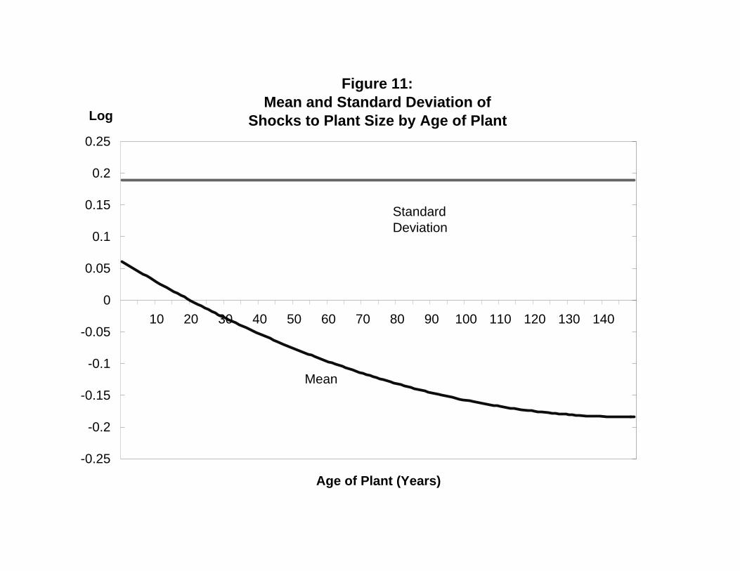
Figure 11:Mean and Standard Deviation of

Shocks to Plant Size by Age of Plant

-0.25

-0.2

-0.15

-0.1

-0.05

0

0.05

0.1

0.15

0.2

0.25

10 20 30 40 50 60 70 80 90 100 110 120 130 140

Age of Plant (Years)

Log

-0.25

-0.2

-0.15

-0.1

-0.05

0

0.05

0.1

0.15

0.2

0.25

Standard Deviation

Mean

Figure 12:Output per Hour in the

Model and the U.S. Data, 1869–1969

2.0

2.5

3.0

3.5

4.0

4.5

5.0

5.5

1860 1880 1900 1920 1940 1960 1980

Year

Lo

g o

f o

utp

ut

per

ho

ur

2

2.5

3

3.5

4

4.5

5

5.5

Trend growth 1869–99: Model 1.6%, Data 1.6%

Trend growth 1899–1929: Model 2.4%, Data 2.6%

Trend growth 1949–69: Model 3.3%, Data 3.3%

Model

Data

Figure 13: Diffusion of New Technology, 1869–1939Model: (% of output produced in plants with new blueprints) vs.Data: (% of horsepower from electric motors in U.S. plants)

0

10

20

30

40

50

60

70

80

90

100

1869 1879 1889 1899 1909 1919 1929 1939

Per

cen

t

0

10

20

30

40

50

60

70

80

90

100

Data

Model