The total cross section at the LHC†

We do not have the ability to perform precise calculations of long-range stronginteraction effects, because the effective QCD coupling is not small and so wecannot use perturbation theory. Nevertheless, I will show that we know a lot,though not nearly enough. As a measure of our lack of knowledge, the bestprediction for the total cross section at LHC energy is:

σLHC = 125 ± 25 mb

This set of lectures is about the long-range strong interaction at high energy.Much of what I know about this subject comes from my long collaborationwith Sandy Donnachie. A few years ago we wrote a book about it, togetherwith colleagues from Heidelberg University: Sandy Donnachie, Gunter Dosch,Peter Landshoff and Otto Nachtmann, Pomeron physics and QCD, CambridgeUniversity Press (2002). Most of the material in these lectures is taken fromthe book, and references to papers and data may be found in it.

†Lectures at School on QCD, Calabria, July 2007

Regge theory

Because we do not have the ability to perform precise calculations of long-range strong interaction effects, much of what we know comes from looking atexperimental data, and so these lectures contain rather more data plots thanequations. In order to use what understanding we have of the theory andapply it to the data, we have to introduce extra assumptions. I will show youthat, often, making the simplest possible assumptions turns out to be verysuccessful.

The basic theory is known as Regge theory. It relates together a large numberof different reactions. Among those that I will discuss are

• Hadron-hadron total cross sections

• Hadron-hadron elastic scattering

• Diffraction dissociation

• Photon and lepton induced reactions

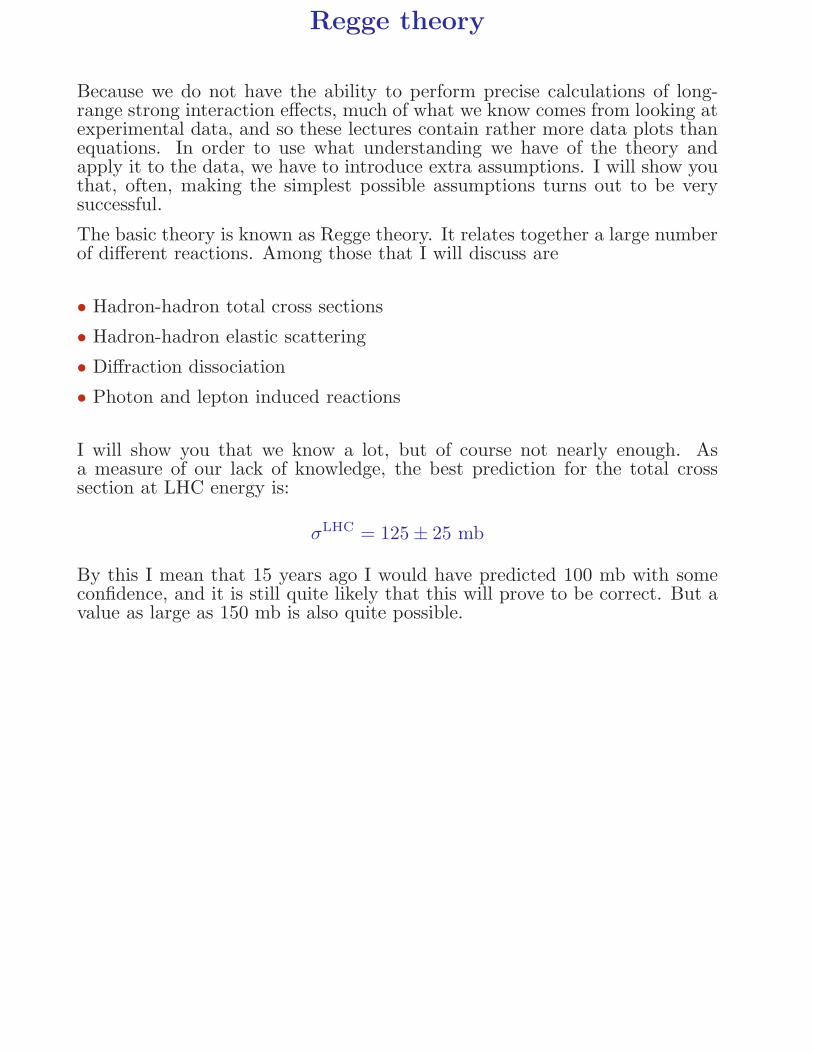
I will show you that we know a lot, but of course not nearly enough. Asa measure of our lack of knowledge, the best prediction for the total crosssection at LHC energy is:

σLHC = 125 ± 25 mb

By this I mean that 15 years ago I would have predicted 100 mb with someconfidence, and it is still quite likely that this will prove to be correct. But avalue as large as 150 mb is also quite possible.

History

• 1935: Yukawa predicted the existence of the pion — itsexchange generates the static strong interaction

• 1960s: Nearly everybody worked on the applications of Regge theory, whichsums the exchanges of many particles and generates the high-energy stronginteraction

• The known particles not are enough — we need to include exchange ofanother object, the pomeron

• 1970s: QCD is discovered — the BFKL equation generates pomeron ex-change as gluon exchange, but it makes total cross sections rise with energymuch faster than is observed

• early 1990s: HERA finds a sharp rise of F2(x,Q2) at small x, apparently

described by BFKL pomeron exchange

• so there are two pomerons: soft (nonperturbative) and hard (perturbative)

• late 1990s: higher-order perturbative corrections to BFKL exchange spoilthe calculation — this problem is not yet solved, and we do not know whetherthe hard pomeron is related to the BFKL equation.

Diffraction

The mathematics to study pomeron exchange is sophisticated andsimilar to that used to study diffraction in optics.

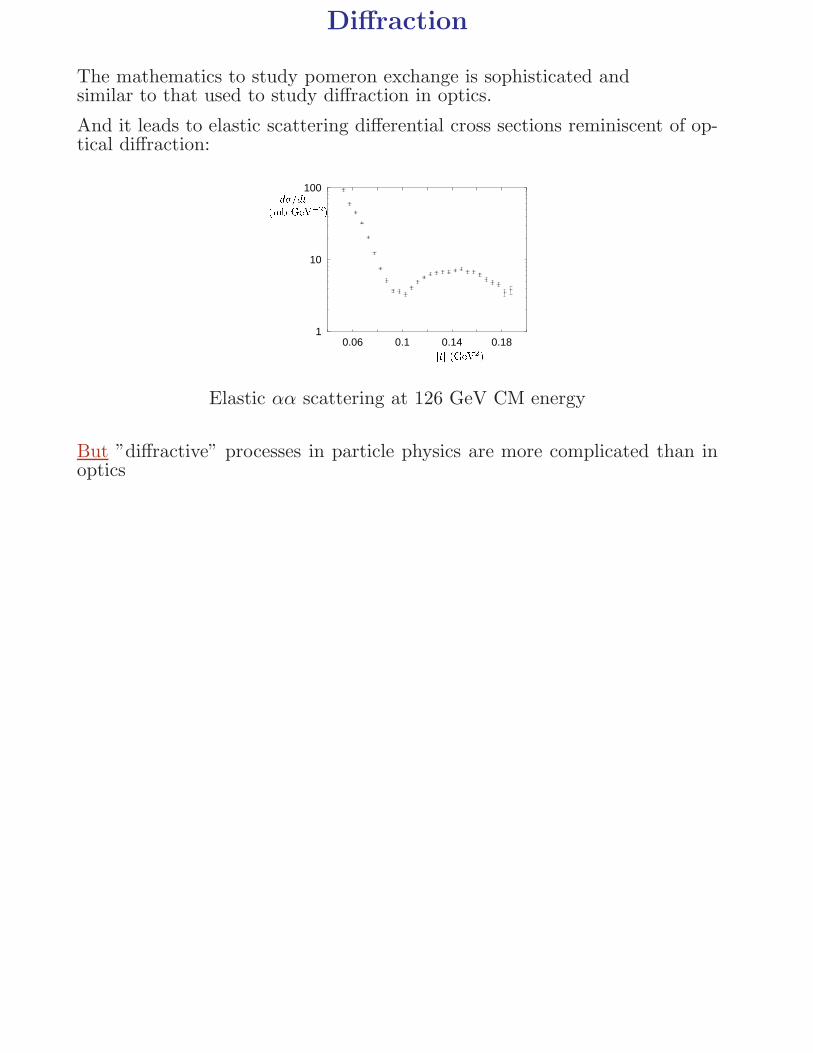
And it leads to elastic scattering differential cross sections reminiscent of op-tical diffraction:

1

10

100

0.06 0.1 0.14 0.18

d�=dt(mb GeV�2)jtj (GeV2)

Elastic αα scattering at 126 GeV CM energy

But ”diffractive” processes in particle physics are more complicated than inoptics

Linear particle trajectories

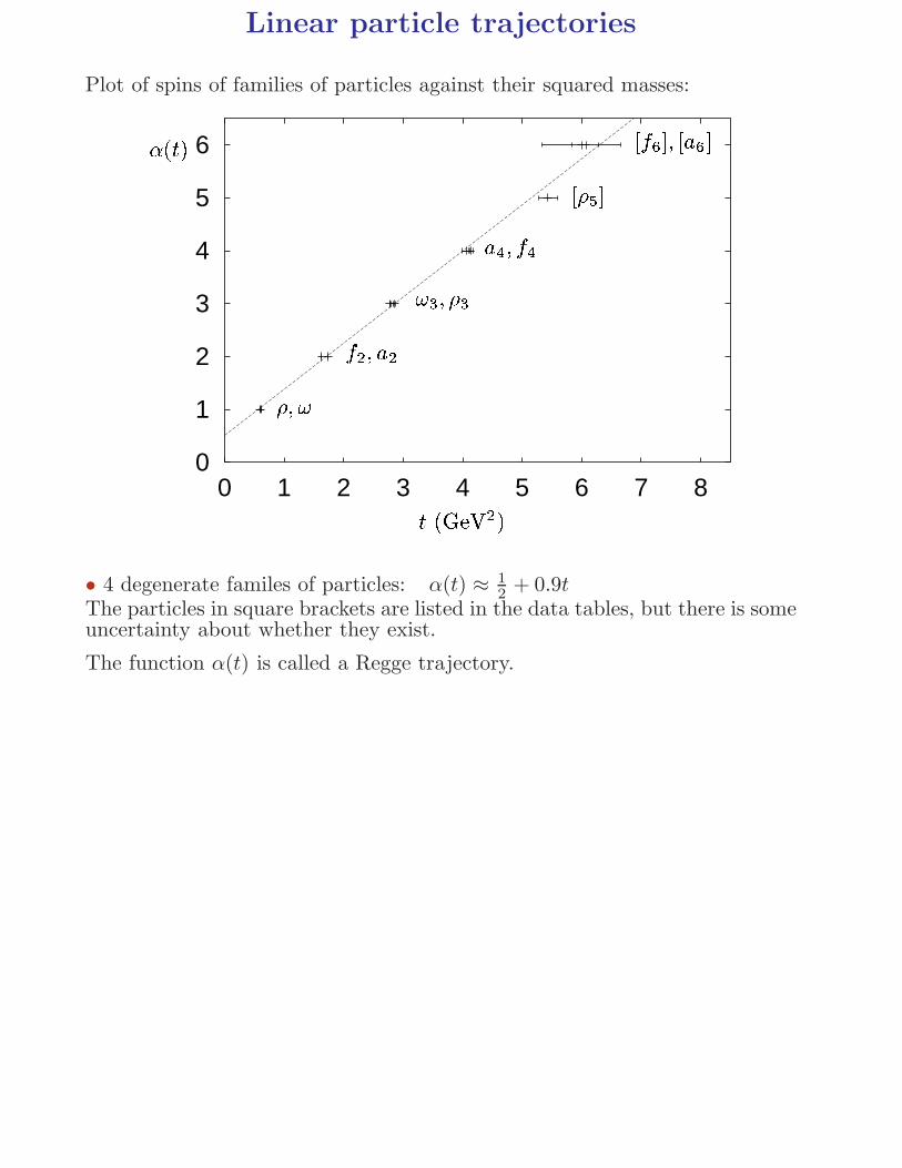
Plot of spins of families of particles against their squared masses:

0

1

2

3

4

5

6

0 1 2 3 4 5 6 7 8t (GeV2)

�(t)�; ! f2; a2 !3; �3 a4; f4 [�5℄ [f6℄; [a6℄

• 4 degenerate familes of particles: α(t) ≈ 12

+ 0.9tThe particles in square brackets are listed in the data tables, but there is someuncertainty about whether they exist.

The function α(t) is called a Regge trajectory.

Regge theory

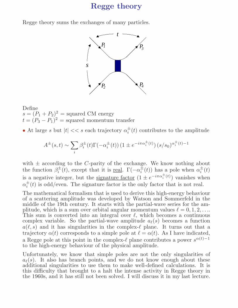
Regge theory sums the exchanges of many particles.

��������������������������������������������������������������������������������������������������

��������������������������������������������������������������������������������������������������

��������������������������������������������������������������������������������������������������

��������������������������������������������������������������������������������������������������

��������������������������������

��������������������������������

������������������������������������

������������������������������������

��������������������������������������������������������������������������������������������������

��������������������������������������������������������������������������������������������������

��������������������������������������������������������������������������������������������������

��������������������������������������������������������������������������������������������������

��������������������������������

��������������������������������

��������������������������������

��������������������������������

s

t

P P

P P

13

2 4

Defines = (P1 + P2)

2 = squared CM energyt = (P3 − P1)

2 = squared momentum transfer

• At large s but |t| << s each trajectory α±

i (t) contributes to the amplitude

A±(s, t) ∼∑

i

β±

i (t)Γ(−α±

i (t)) (1 ± e−iπα±

i(t)) (s/s0)

α±

i(t)−1

with ± according to the C-parity of the exchange. We know nothing aboutthe function β±

i (t), except that it is real. Γ(−α±

i (t)) has a pole when α±

i (t)

is a negative integer, but the signature factor (1 ± e−iπα±

i(t)) vanishes when

α±

i (t) is odd/even. The signature factor is the only factor that is not real.

The mathematical formalism that is used to derive this high-energy behaviourof a scattering amplitude was developed by Watson and Sommerfeld in themiddle of the 19th century. It starts with the partial-wave series for the am-plitude, which is a sum over orbital angular momentum values ℓ = 0, 1, 2, . . ..This sum is converted into an integral over ℓ, which becomes a continuouscomplex variable. So the partial-wave amplitude aℓ(s) becomes a functiona(ℓ, s) and it has singularities in the complex-ℓ plane. It turns out that atrajectory α(t) corresponds to a simple pole at ℓ = α(t). As I have indicated,a Regge pole at this point in the complex-ℓ plane contributes a power sα(t)−1

to the high-energy behaviour of the physical amplitude.

Unfortunately, we know that simple poles are not the only singularities ofaℓ(s). It also has branch points, and we do not know enough about theseadditional singularities to use them to make well-defined calculations. It isthis difficulty that brought to a halt the intense activity in Regge theory inthe 1960s, and it has still not been solved. I will discuss it in my last lecture.

Total cross sections

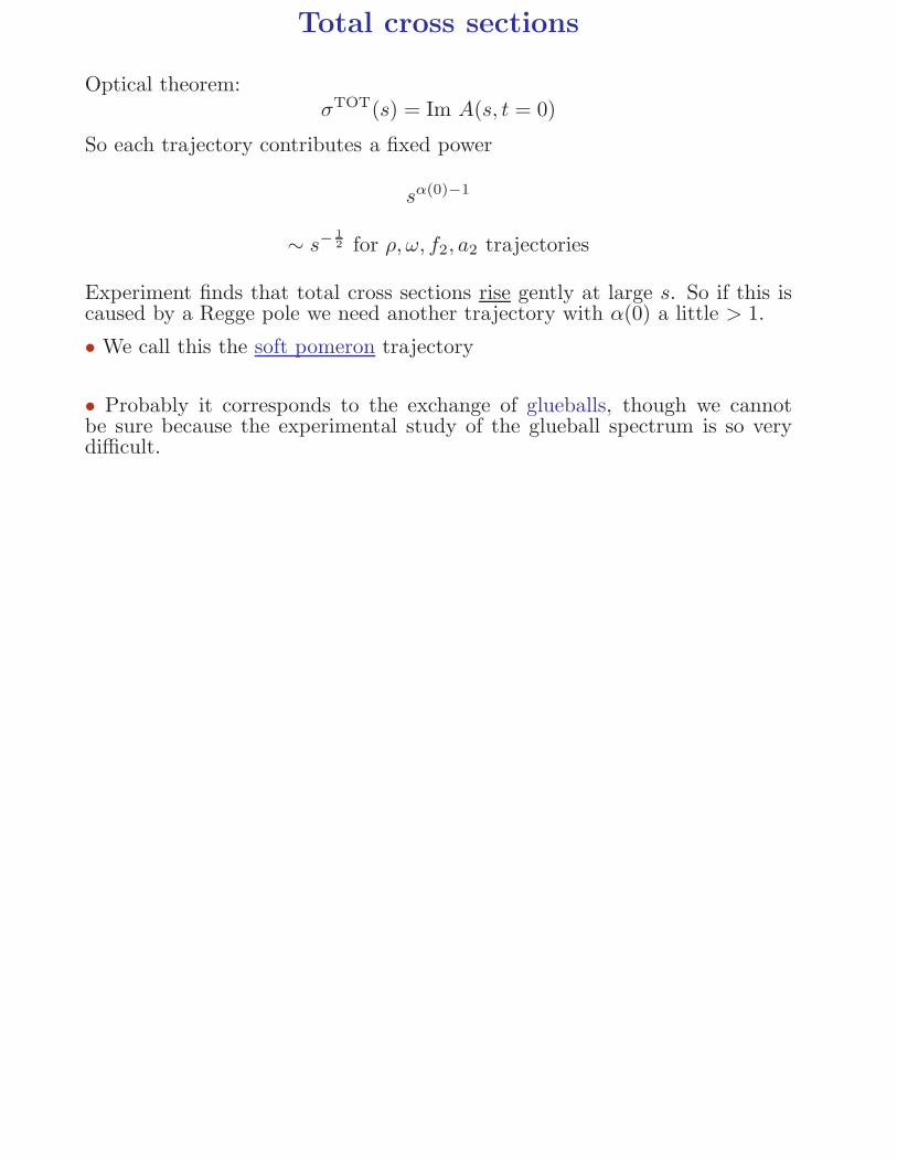
Optical theorem:σTOT(s) = Im A(s, t = 0)

So each trajectory contributes a fixed power

sα(0)−1

∼ s−1

2 for ρ, ω, f2, a2 trajectories

Experiment finds that total cross sections rise gently at large s. So if this iscaused by a Regge pole we need another trajectory with α(0) a little > 1.

• We call this the soft pomeron trajectory

• Probably it corresponds to the exchange of glueballs, though we cannotbe sure because the experimental study of the glueball spectrum is so verydifficult.

Fits to total cross sections

30

40

50

60

70

80

10 100 1000

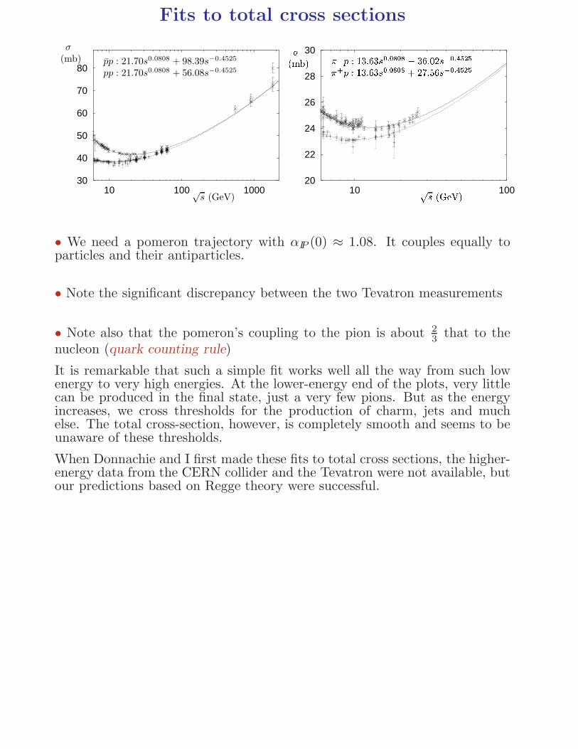
pp : 21.70s0.0808 + 98.39s−0.4525

pp : 21.70s0.0808 + 56.08s−0.4525

σ(mb)

√s (GeV)

20

22

24

26

28

30

10 100

��p : 13:63s0:0808 + 36:02s�0:4525�+p : 13:63s0:0808 + 27:56s�0:4525�(mb)ps (GeV)

• We need a pomeron trajectory with αIP (0) ≈ 1.08. It couples equally toparticles and their antiparticles.

• Note the significant discrepancy between the two Tevatron measurements

• Note also that the pomeron’s coupling to the pion is about 23

that to thenucleon (quark counting rule)

It is remarkable that such a simple fit works well all the way from such lowenergy to very high energies. At the lower-energy end of the plots, very littlecan be produced in the final state, just a very few pions. But as the energyincreases, we cross thresholds for the production of charm, jets and muchelse. The total cross-section, however, is completely smooth and seems to beunaware of these thresholds.

When Donnachie and I first made these fits to total cross sections, the higher-energy data from the CERN collider and the Tevatron were not available, butour predictions based on Regge theory were successful.

16

18

20

22

24

26

10 100

K�p : 11:93s0:0808 + 25:33s�0:4525K+p : 11:93s0:0808 + 7:58s�0:4525�(mb)ps (GeV) 35

40

45

50

10 100

�pn : 21:70s0:0808 + 92:71s�0:4525pn : 21:70s0:0808 + 54:77s�0:4525�(mb)ps (GeV)

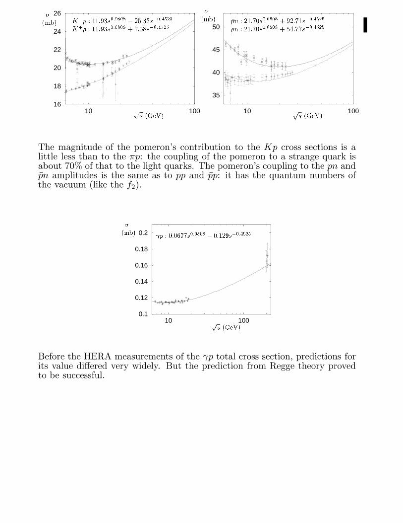
The magnitude of the pomeron’s contribution to the Kp cross sections is alittle less than to the πp: the coupling of the pomeron to a strange quark isabout 70% of that to the light quarks. The pomeron’s coupling to the pn andpn amplitudes is the same as to pp and pp: it has the quantum numbers ofthe vacuum (like the f2).

0.1

0.12

0.14

0.16

0.18

0.2

10 100

p : 0:0677s0:0808 + 0:129s�0:4525�(mb)ps (GeV)

Before the HERA measurements of the γp total cross section, predictions forits value differed very widely. But the prediction from Regge theory provedto be successful.

Froissart-Lukaszuk-Martin bound

At very large s

σTOT(s) <π

m2π

log2(s/s0)

for some unknown s0 — probably of the order of 1 GeV2.

At LHC energy, this gives σTOT < 4.3 barns

• So the bound has little to do with physics!

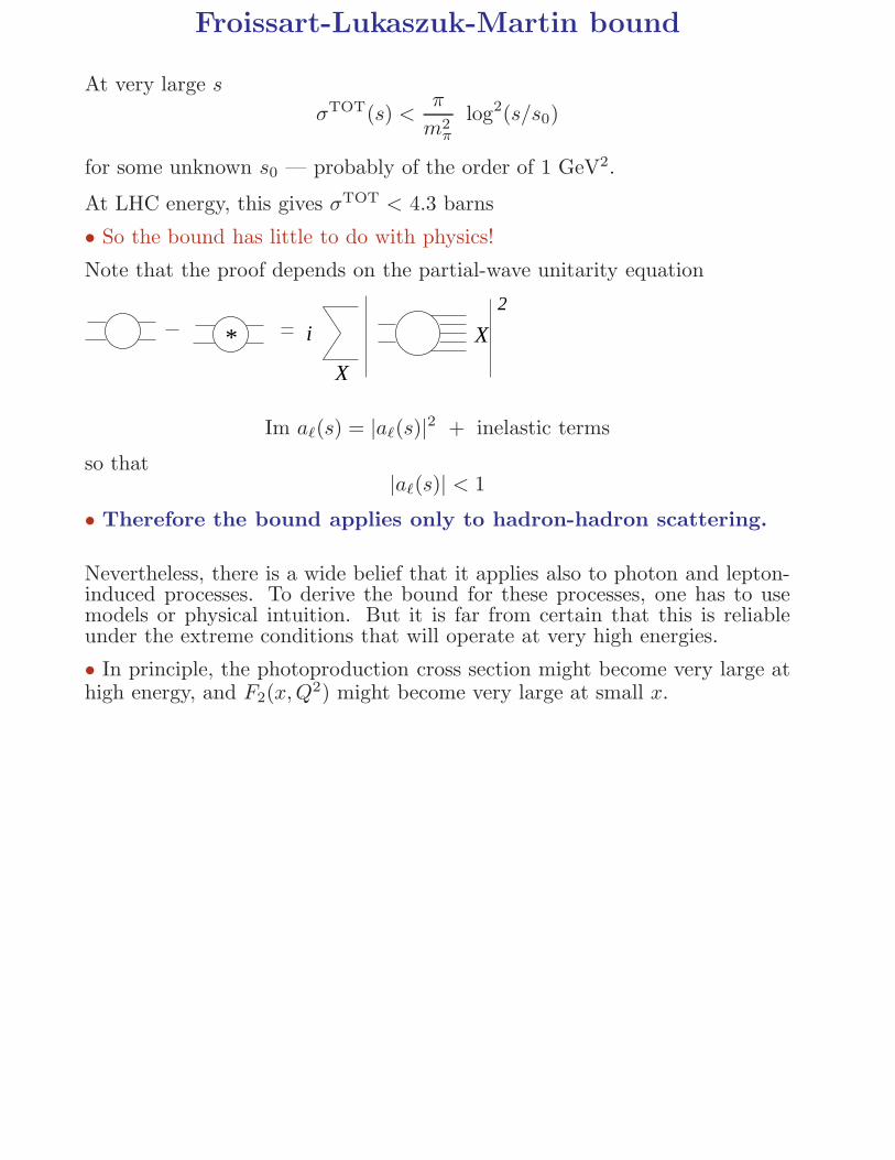
Note that the proof depends on the partial-wave unitarity equation

*

2

X

Xi

Im aℓ(s) = |aℓ(s)|2 + inelastic terms

so that|aℓ(s)| < 1

• Therefore the bound applies only to hadron-hadron scattering.

Nevertheless, there is a wide belief that it applies also to photon and lepton-induced processes. To derive the bound for these processes, one has to usemodels or physical intuition. But it is far from certain that this is reliableunder the extreme conditions that will operate at very high energies.

• In principle, the photoproduction cross section might become very large athigh energy, and F2(x,Q

2) might become very large at small x.

A more stringent constraint

ObviouslyσELASTIC < σTOTAL

In fact, unitarity can be used to show that even

σELASTIC < 12 σ

TOTAL

This is the Pumplin Bound.

Because pomeron exchange alone gives

σTOTAL ∼ sǫ ǫ ≈ 0.08

anddσ

dt

ELASTIC∣

∣

∣

t=0∼ s2ǫ

it violates the bound at large s.

More about this later.

Elastic scattering

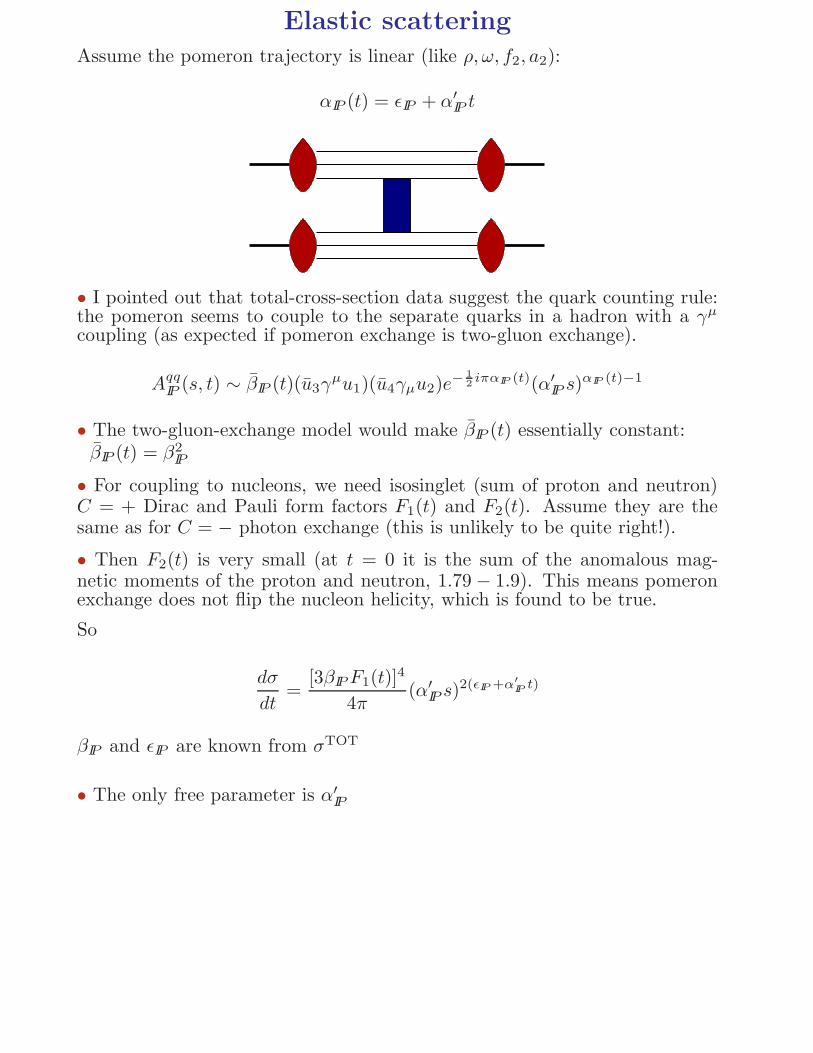
Assume the pomeron trajectory is linear (like ρ, ω, f2, a2):

αIP (t) = ǫIP + α′

IP t

• I pointed out that total-cross-section data suggest the quark counting rule:the pomeron seems to couple to the separate quarks in a hadron with a γµ

coupling (as expected if pomeron exchange is two-gluon exchange).

AqqIP (s, t) ∼ βIP (t)(u3γ

µu1)(u4γµu2)e−

1

2iπαIP (t)(α′

IP s)αIP (t)−1

• The two-gluon-exchange model would make βIP (t) essentially constant:βIP (t) = β2

IP

• For coupling to nucleons, we need isosinglet (sum of proton and neutron)C = + Dirac and Pauli form factors F1(t) and F2(t). Assume they are thesame as for C = − photon exchange (this is unlikely to be quite right!).

• Then F2(t) is very small (at t = 0 it is the sum of the anomalous mag-netic moments of the proton and neutron, 1.79 − 1.9). This means pomeronexchange does not flip the nucleon helicity, which is found to be true.

So

dσ

dt=

[3βIPF1(t)]4

4π(α′

IP s)2(ǫIP +α′

IPt)

βIP and ǫIP are known from σTOT

• The only free parameter is α′IP

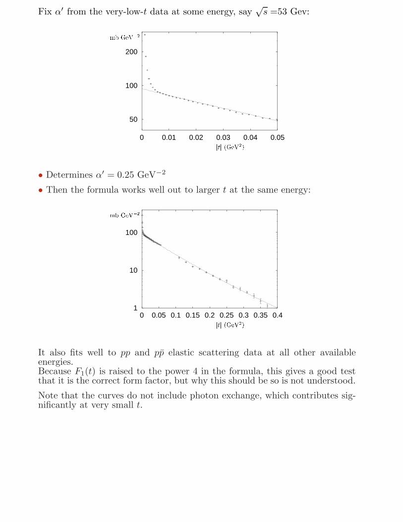
Fix α′ from the very-low-t data at some energy, say√s =53 Gev:

50

100

200

0 0.01 0.02 0.03 0.04 0.05jtj (GeV2)

mb GeV�2

• Determines α′ = 0.25 GeV−2

• Then the formula works well out to larger t at the same energy:

1

10

100

0 0.05 0.1 0.15 0.2 0.25 0.3 0.35 0.4jtj (GeV2)

mb GeV�2

It also fits well to pp and pp elastic scattering data at all other availableenergies.Because F1(t) is raised to the power 4 in the formula, this gives a good testthat it is the correct form factor, but why this should be so is not understood.

Note that the curves do not include photon exchange, which contributes sig-nificantly at very small t.

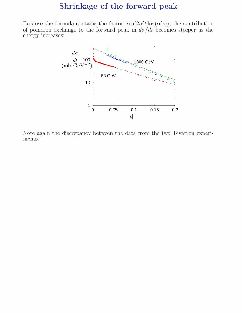
Shrinkage of the forward peak

Because the formula contains the factor exp(2α′t log(α′s)), the contributionof pomeron exchange to the forward peak in dσ/dt becomes steeper as theenergy increases:

1

10

100

0 0.05 0.1 0.15 0.2

53 GeV

1800 GeV

|t|

dσ

dt(mb GeV−2)

Note again the discrepancy between the data from the two Tevatron experi-ments.

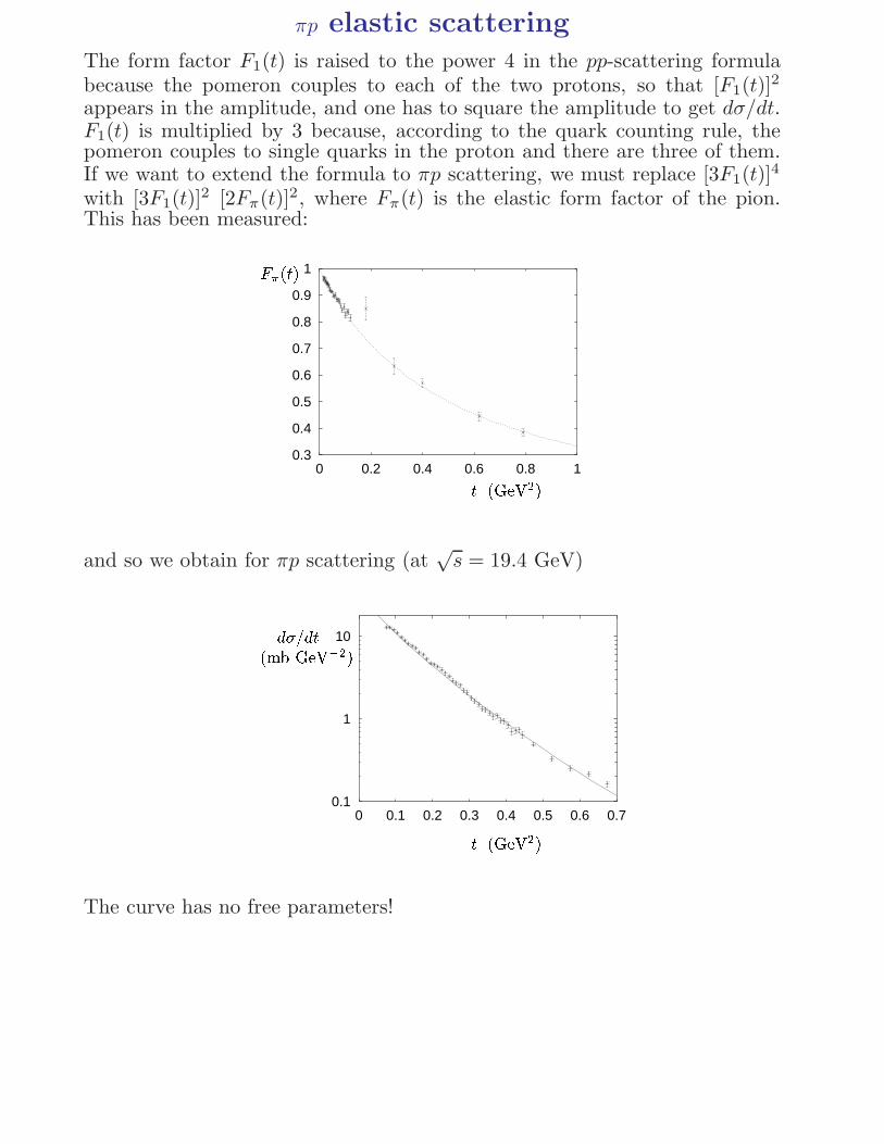
πp elastic scattering

The form factor F1(t) is raised to the power 4 in the pp-scattering formulabecause the pomeron couples to each of the two protons, so that [F1(t)]

2

appears in the amplitude, and one has to square the amplitude to get dσ/dt.F1(t) is multiplied by 3 because, according to the quark counting rule, thepomeron couples to single quarks in the proton and there are three of them.If we want to extend the formula to πp scattering, we must replace [3F1(t)]

4

with [3F1(t)]2 [2Fπ(t)]2, where Fπ(t) is the elastic form factor of the pion.

This has been measured:

0.3

0.4

0.5

0.6

0.7

0.8

0.9

1

0 0.2 0.4 0.6 0.8 1

F�(t)jtj (GeV2)

and so we obtain for πp scattering (at√s = 19.4 GeV)

0.1

1

10

0 0.1 0.2 0.3 0.4 0.5 0.6 0.7jtj (GeV2)d�=dt(mb GeV�2)

The curve has no free parameters!

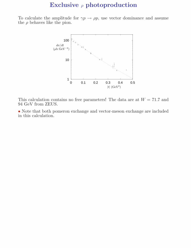
Exclusive ρ photoproduction

To calculate the amplitude for γp → ρp, use vector dominance and assumethe ρ behaves like the pion.

1

10

100

0 0.1 0.2 0.3 0.4 0.5

dσ/dt(µb GeV−2)

|t| (GeV2)

This calculation contains no free parameters! The data are at W = 71.7 and94 GeV from ZEUS.

• Note that both pomeron exchange and vector-meson exchange are includedin this calculation.

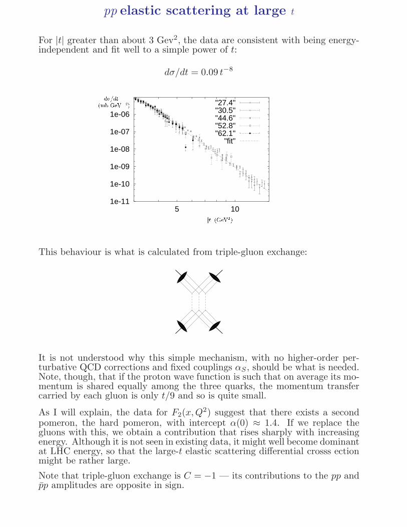
pp elastic scattering at large t

For |t| greater than about 3 Gev2, the data are consistent with being energy-independent and fit well to a simple power of t:

dσ/dt = 0.09 t−8

1e-11

1e-10

1e-09

1e-08

1e-07

1e-06

5 10

"27.4""30.5""44.6""52.8""62.1"

"fit"

d�=dt(mb GeV�2)

jtj (GeV2)This behaviour is what is calculated from triple-gluon exchange:

It is not understood why this simple mechanism, with no higher-order per-turbative QCD corrections and fixed couplings αS , should be what is needed.Note, though, that if the proton wave function is such that on average its mo-mentum is shared equally among the three quarks, the momentum transfercarried by each gluon is only t/9 and so is quite small.

As I will explain, the data for F2(x,Q2) suggest that there exists a second

pomeron, the hard pomeron, with intercept α(0) ≈ 1.4. If we replace thegluons with this, we obtain a contribution that rises sharply with increasingenergy. Although it is not seen in existing data, it might well become dominantat LHC energy, so that the large-t elastic scattering differential crosss ectionmight be rather large.

Note that triple-gluon exchange is C = −1 — its contributions to the pp andpp amplitudes are opposite in sign.

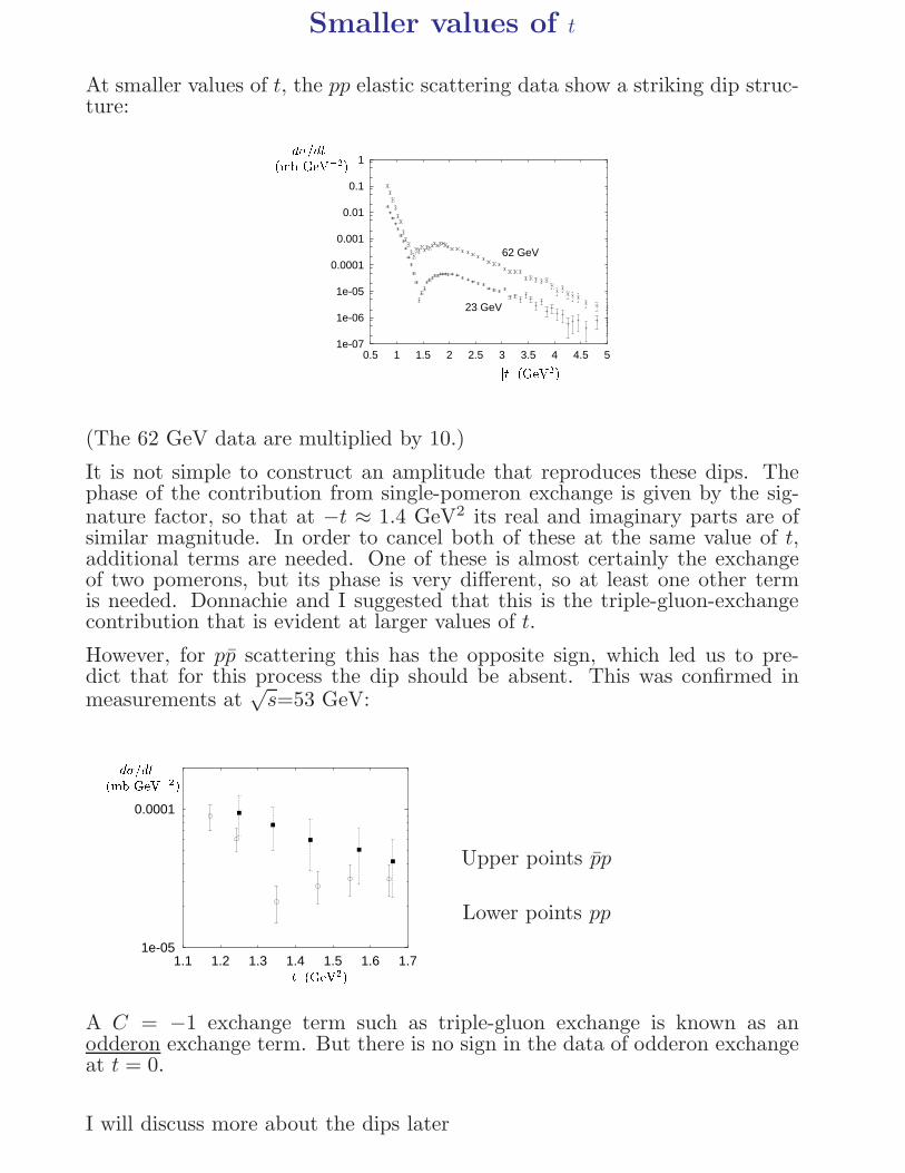
Smaller values of t

At smaller values of t, the pp elastic scattering data show a striking dip struc-ture:

1e-07

1e-06

1e-05

0.0001

0.001

0.01

0.1

1

0.5 1 1.5 2 2.5 3 3.5 4 4.5 5

62 GeV

23 GeV

d�=dt(mb GeV�2)

jtj (GeV2)(The 62 GeV data are multiplied by 10.)

It is not simple to construct an amplitude that reproduces these dips. Thephase of the contribution from single-pomeron exchange is given by the sig-nature factor, so that at −t ≈ 1.4 GeV2 its real and imaginary parts are ofsimilar magnitude. In order to cancel both of these at the same value of t,additional terms are needed. One of these is almost certainly the exchangeof two pomerons, but its phase is very different, so at least one other termis needed. Donnachie and I suggested that this is the triple-gluon-exchangecontribution that is evident at larger values of t.

However, for pp scattering this has the opposite sign, which led us to pre-dict that for this process the dip should be absent. This was confirmed inmeasurements at

√s=53 GeV:

1e-05

0.0001

1.1 1.2 1.3 1.4 1.5 1.6 1.7

d�=dt(mb GeV�2)

jtj (GeV2)Upper points pp

Lower points pp

A C = −1 exchange term such as triple-gluon exchange is known as anodderon exchange term. But there is no sign in the data of odderon exchangeat t = 0.

I will discuss more about the dips later

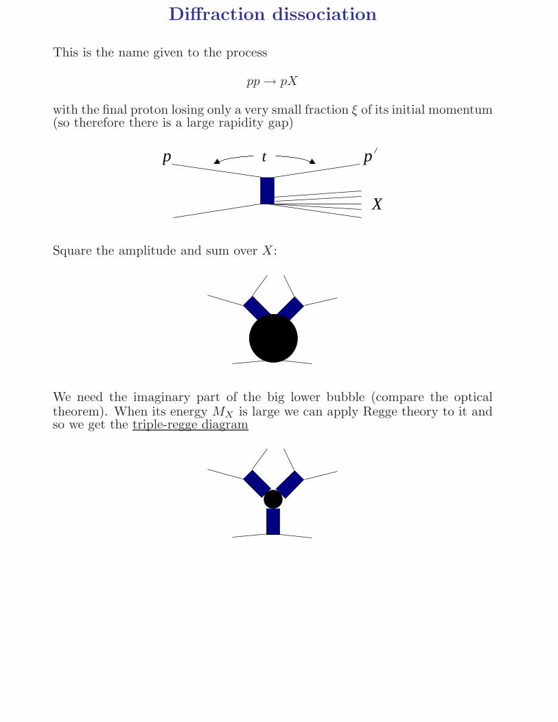
Diffraction dissociation

This is the name given to the process

pp→ pX

with the final proton losing only a very small fraction ξ of its initial momentum(so therefore there is a large rapidity gap)

t pp

X

Square the amplitude and sum over X:

We need the imaginary part of the big lower bubble (compare the opticaltheorem). When its energy MX is large we can apply Regge theory to it andso we get the triple-regge diagram

t t

t=0

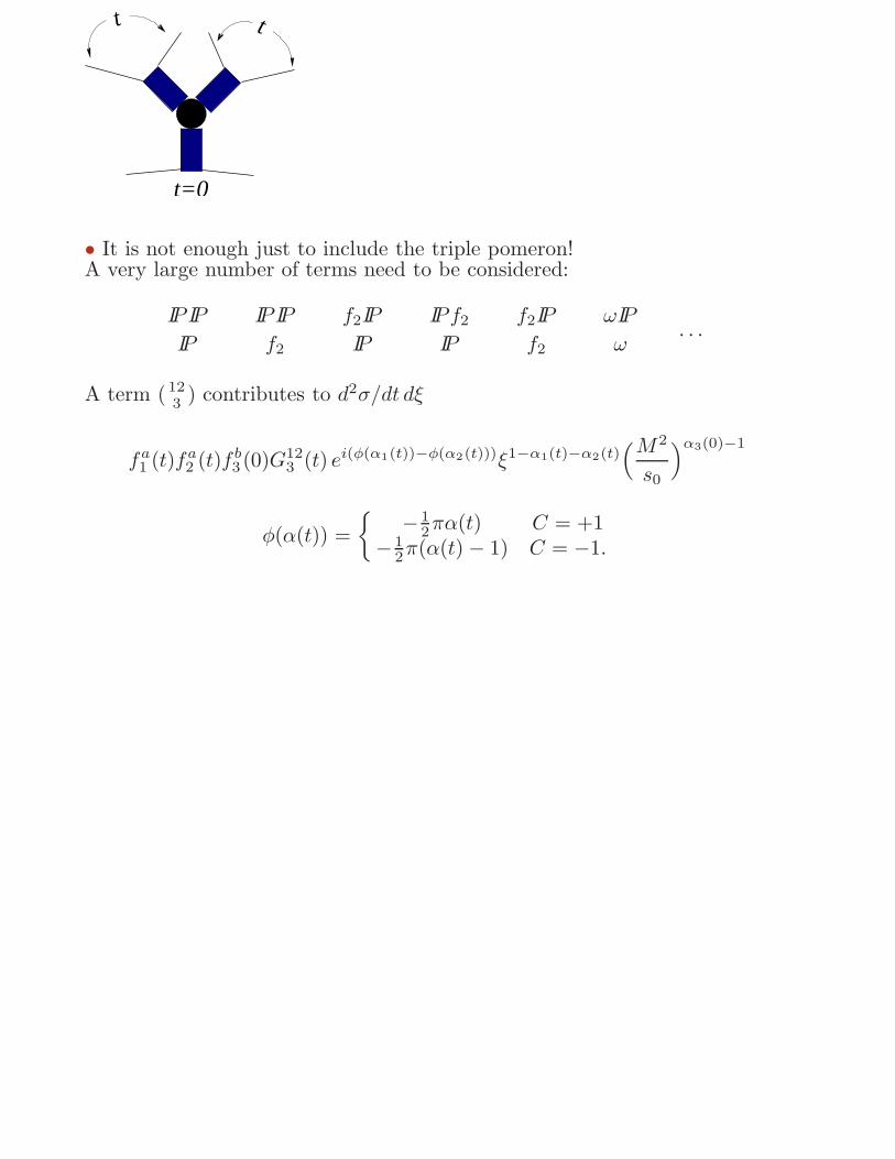
• It is not enough just to include the triple pomeron!A very large number of terms need to be considered:

IPIP

IP

IPIP

f2

f2IP

IP

IPf2IP

f2IP

f2

ωIP

ω. . .

A term (123 ) contributes to d2σ/dt dξ

fa1 (t)fa

2 (t)f b3 (0)G12

3 (t) ei(φ(α1(t))−φ(α2(t)))ξ1−α1(t)−α2(t)(M2

s0

)α3(0)−1

φ(α(t)) =

{

−12πα(t) C = +1

−12π(α(t) − 1) C = −1.

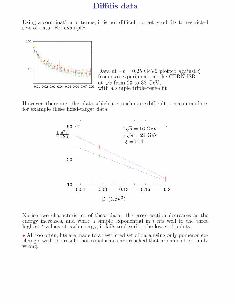
Diffdis data

Using a combination of terms, it is not difficult to get good fits to restrictedsets of data. For example:

10

100

0.01 0.02 0.03 0.04 0.05 0.06 0.07 0.08

Data at −t = 0.25 GeV2 plotted against ξfrom two experiments at the CERN ISRat

√s from 23 to 38 GeV,

with a simple triple-regge fit

However, there are other data which are much more difficult to accommodate,for example these fixed-target data:

50

20

100.20.160.120.080.04

|t| (GeV2)

1π

d2σdtdξ

√s = 16 GeV√s = 24 GeV

ξ =0.04

Notice two characteristics of these data: the cross section decreases as theenergy increases, and while a simple exponential in t fits well to the threehighest-t values at each energy, it fails to describe the lowest-t points.

• All too often, fits are made to a restricted set of data using only pomeron ex-change, with the result that conclusions are reached that are almost certainlywrong.

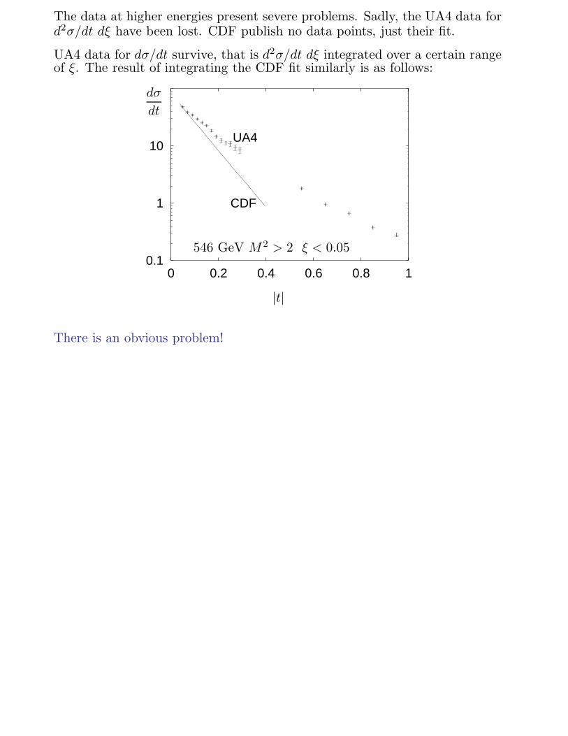
The data at higher energies present severe problems. Sadly, the UA4 data ford2σ/dt dξ have been lost. CDF publish no data points, just their fit.

UA4 data for dσ/dt survive, that is d2σ/dt dξ integrated over a certain rangeof ξ. The result of integrating the CDF fit similarly is as follows:

0.1

1

10

0 0.2 0.4 0.6 0.8 1

UA4

CDF

|t|

dσ

dt

546 GeV M2 > 2 ξ < 0.05

There is an obvious problem!

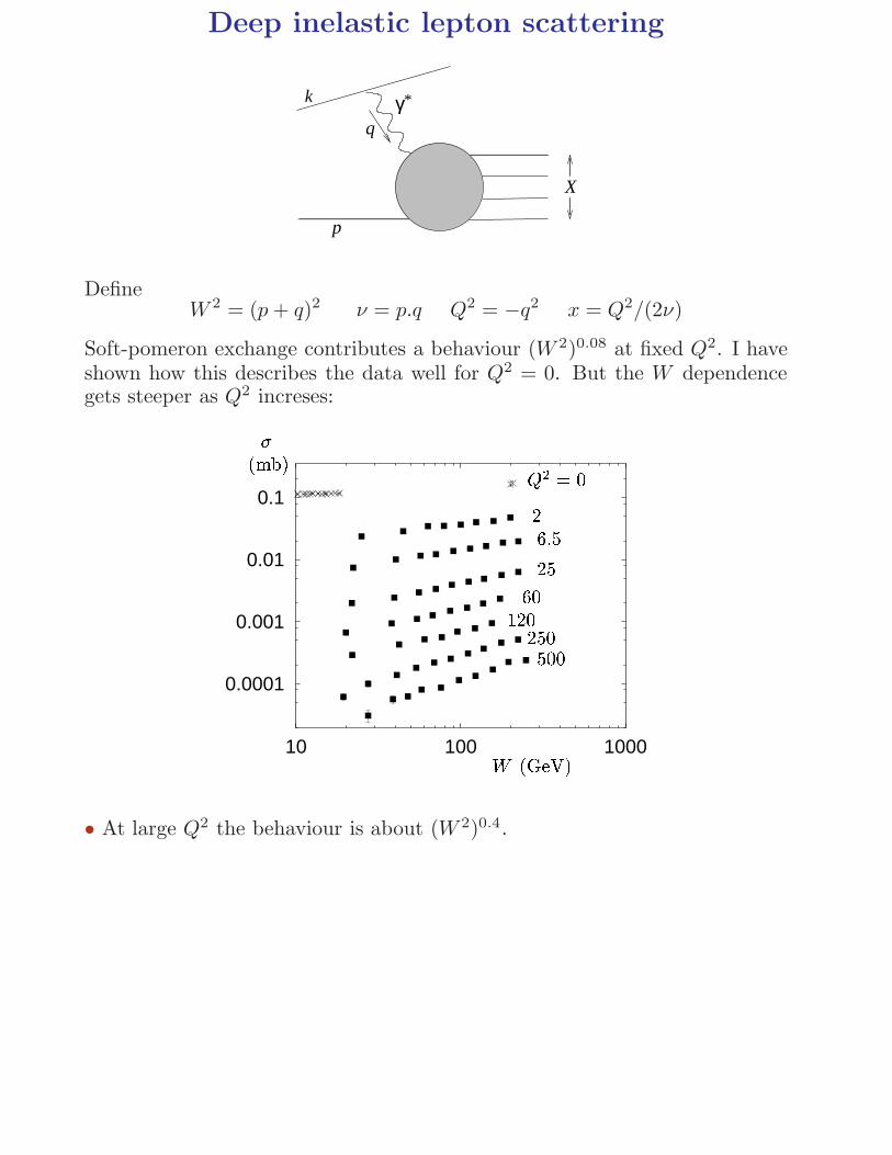
Deep inelastic lepton scattering

*γk

p

q

X

DefineW 2 = (p+ q)2 ν = p.q Q2 = −q2 x = Q2/(2ν)

Soft-pomeron exchange contributes a behaviour (W 2)0.08 at fixed Q2. I haveshown how this describes the data well for Q2 = 0. But the W dependencegets steeper as Q2 increses:

0.0001

0.001

0.01

0.1

10 100 1000

�(mb)

W (GeV)

Q2 = 026.52560120250500• At large Q2 the behaviour is about (W 2)0.4.

The theory is not well understood

Define

σ(W 2, Q2) =4π2α2

EM

Q2F2(x,Q

2)

Two alternative theoretical possibilities:

• A (W 2)0.4 term is there at all Q2, but at Q2 = 0 its contribution is verysmall

• It is not there at Q2 = 0, but as Q2 increases it is gradually generatedthrough perturbative QCD evolution.

The second approach is conventional, but it has a mathematical problem, asI will explain.

The first leads to the possibility that σ(pp) also has an s0.4 term, so that theLHC total cross-section is big.

Simple Regge fit

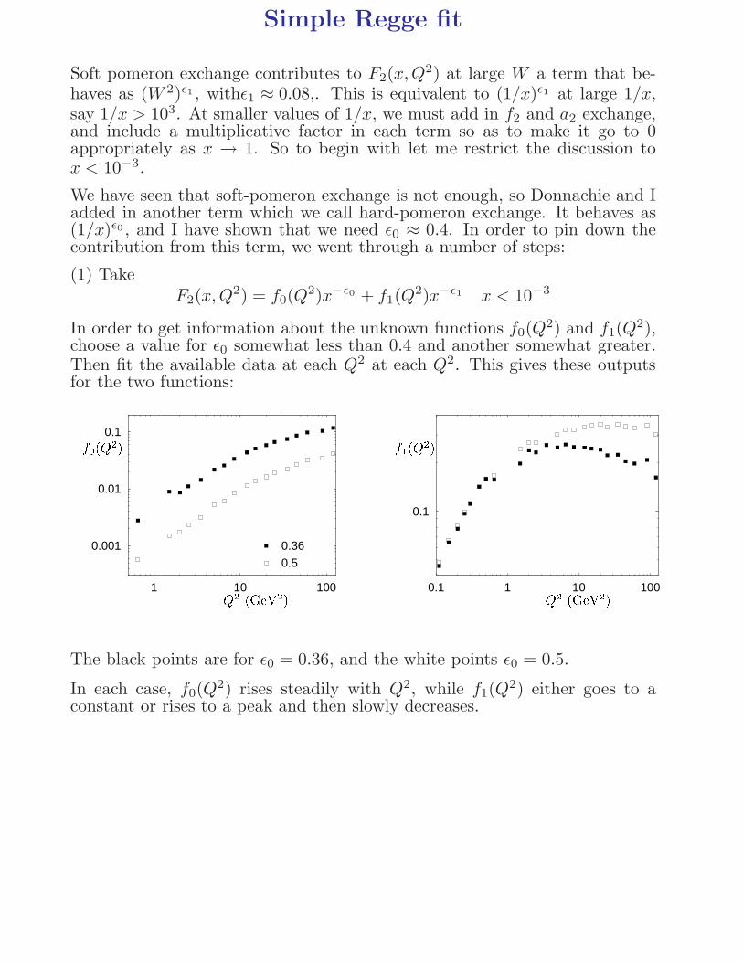
Soft pomeron exchange contributes to F2(x,Q2) at large W a term that be-

haves as (W 2)ǫ1 , withǫ1 ≈ 0.08,. This is equivalent to (1/x)ǫ1 at large 1/x,say 1/x > 103. At smaller values of 1/x, we must add in f2 and a2 exchange,and include a multiplicative factor in each term so as to make it go to 0appropriately as x → 1. So to begin with let me restrict the discussion tox < 10−3.

We have seen that soft-pomeron exchange is not enough, so Donnachie and Iadded in another term which we call hard-pomeron exchange. It behaves as(1/x)ǫ0 , and I have shown that we need ǫ0 ≈ 0.4. In order to pin down thecontribution from this term, we went through a number of steps:

(1) TakeF2(x,Q

2) = f0(Q2)x−ǫ0 + f1(Q

2)x−ǫ1 x < 10−3

In order to get information about the unknown functions f0(Q2) and f1(Q

2),choose a value for ǫ0 somewhat less than 0.4 and another somewhat greater.Then fit the available data at each Q2 at each Q2. This gives these outputsfor the two functions:

0.001

0.01

0.1

1 10 100

0.36

0.5Q2 (GeV2)f0(Q2)

0.1

0.1 1 10 100Q2 (GeV2)f1(Q2)

The black points are for ǫ0 = 0.36, and the white points ǫ0 = 0.5.

In each case, f0(Q2) rises steadily with Q2, while f1(Q

2) either goes to aconstant or rises to a peak and then slowly decreases.

(2) This suggests parametrisations of f0(Q2) and f1(Q

2). Current conserva-tion implies that that near Q2 = 0 at fixed W , F2(x,Q

2) vanishes like Q2.Therefore fi(Q

2) ∼ (Q2)1+ǫi . Take

f0(Q2) = A0

( Q2

1 +Q2/Q20

)1+ǫ0(1 +Q2/Q2

0)ǫ0/2

f1(Q2) = A1

( Q2

1 +Q2/Q21

)1+ǫ1

For simplicity, this choice makes f1(Q2) go to a constant at large Q2.

Although its contribution for x < 0.001 is fairly small, we include also anf2, a2 exchange term, that is we add

fRQ2)x−ǫR ǫR = −0.4525

and use a similar parametrisation for f2(Q2) to that for f1(Q

2):

fR(Q2) = AR

( Q2

1 +Q2/Q2R

)1+ǫR

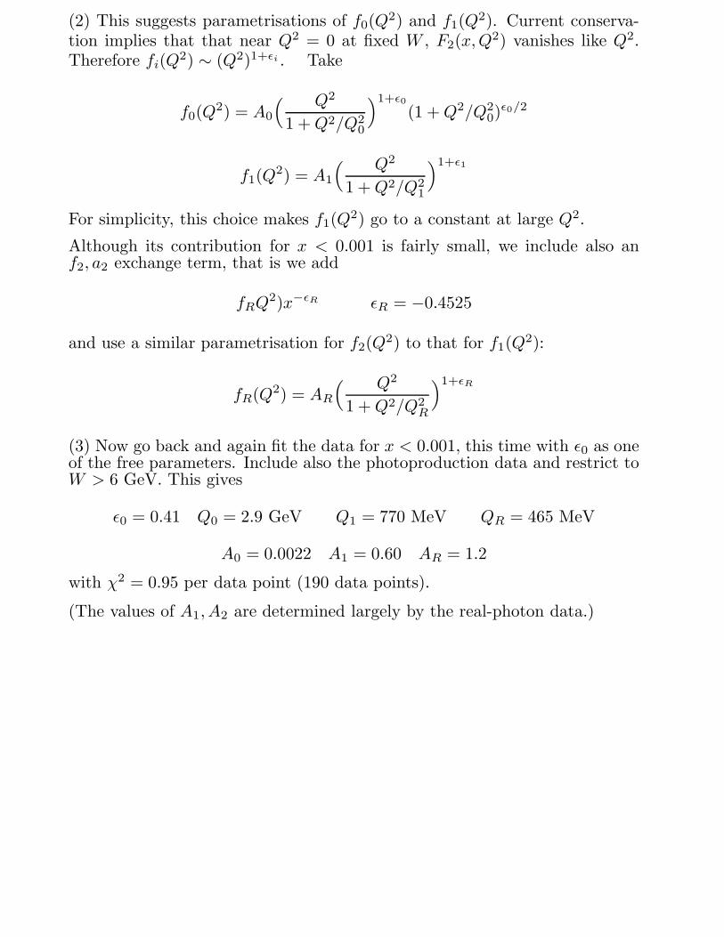
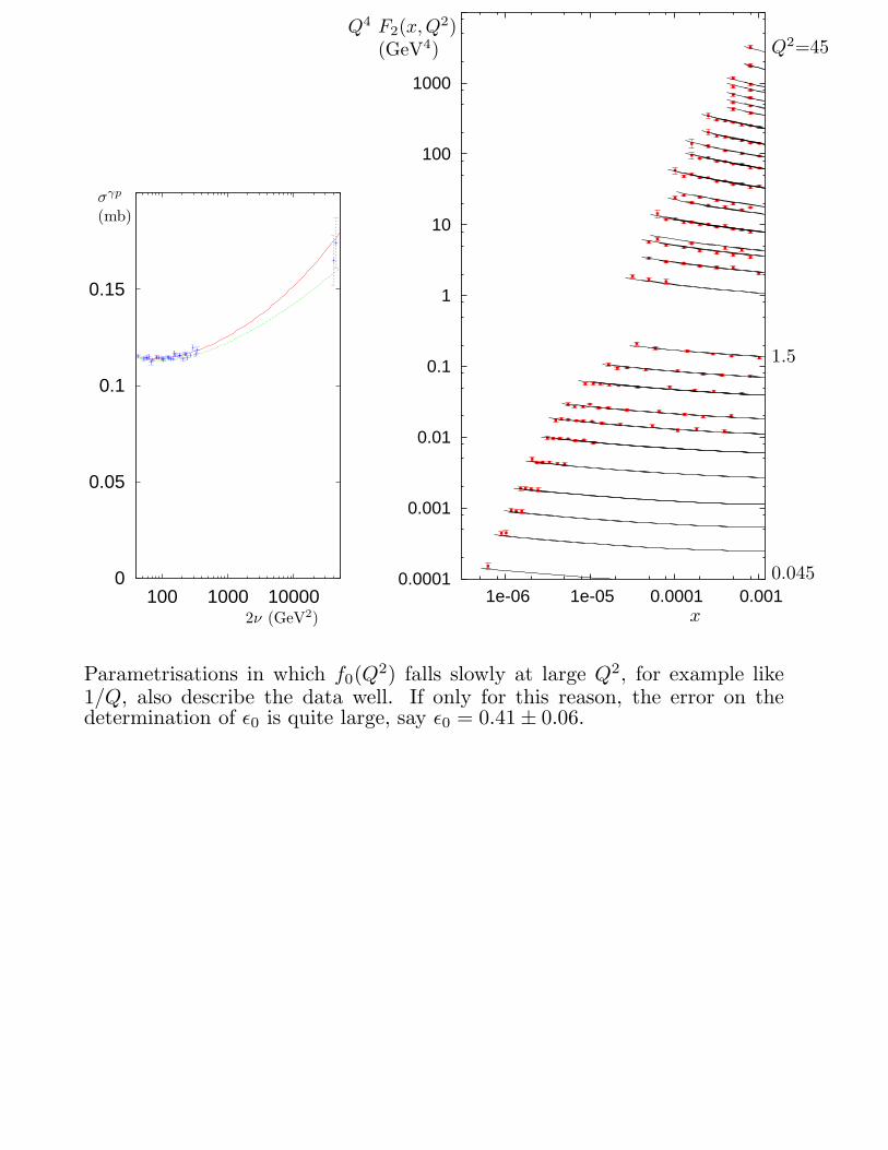
(3) Now go back and again fit the data for x < 0.001, this time with ǫ0 as oneof the free parameters. Include also the photoproduction data and restrict toW > 6 GeV. This gives

ǫ0 = 0.41 Q0 = 2.9 GeV Q1 = 770 MeV QR = 465 MeV

A0 = 0.0022 A1 = 0.60 AR = 1.2

with χ2 = 0.95 per data point (190 data points).

(The values of A1, A2 are determined largely by the real-photon data.)

0

0.05

0.1

0.15

100 1000 100002ν (GeV2)

σγp

(mb)

0.0001

0.001

0.01

0.1

1

10

100

1000

1e-06 1e-05 0.0001 0.001x

Q4 F2(x,Q2)

(GeV4) Q2=45

1.5

0.045

Parametrisations in which f0(Q2) falls slowly at large Q2, for example like

1/Q, also describe the data well. If only for this reason, the error on thedetermination of ǫ0 is quite large, say ǫ0 = 0.41 ± 0.06.

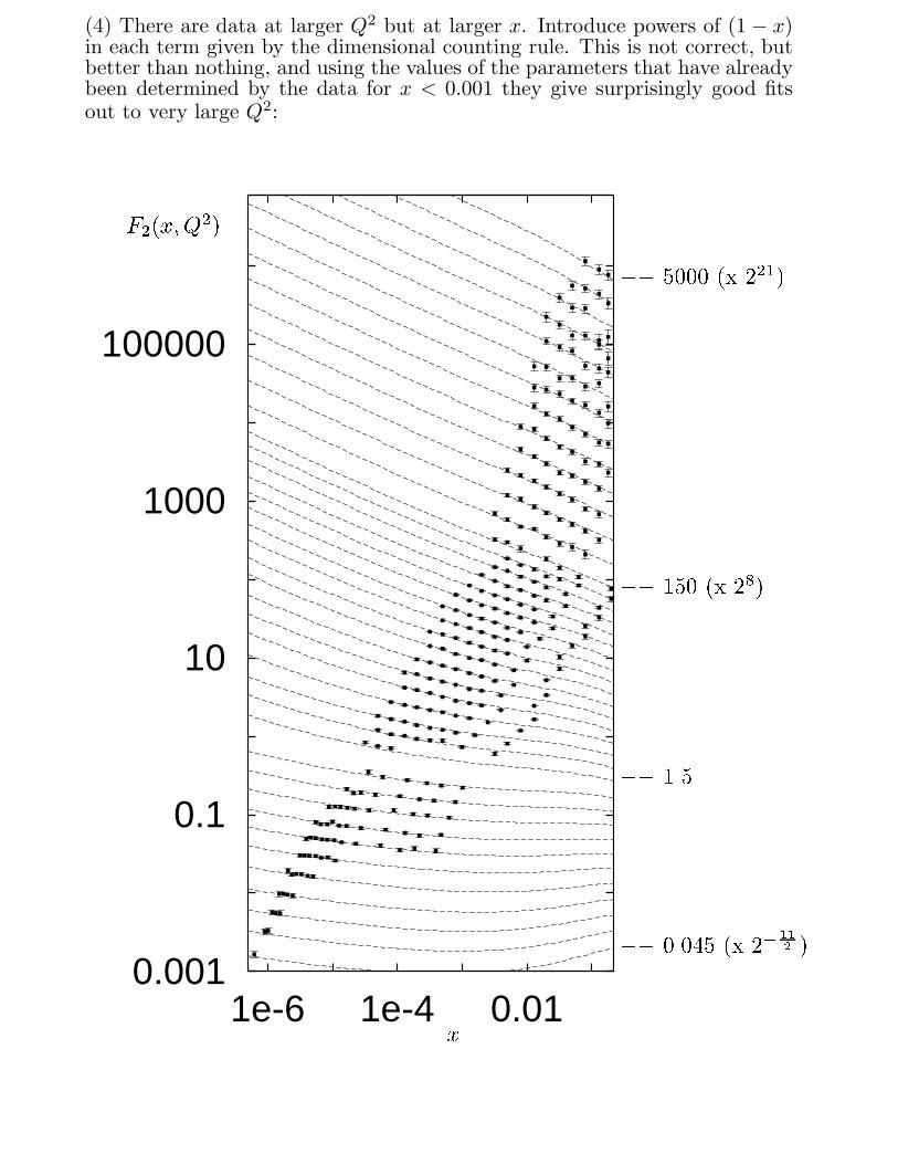
(4) There are data at larger Q2 but at larger x. Introduce powers of (1 − x)in each term given by the dimensional counting rule. This is not correct, butbetter than nothing, and using the values of the parameters that have alreadybeen determined by the data for x < 0.001 they give surprisingly good fitsout to very large Q2:

0.001

0.1

10

1000

100000

1e-6 1e-4 0.01x

F2(x;Q2) �� 5000 (x 221)

�� 150 (x 28)�� 1.5�� 0.045 (x 2� 112 )

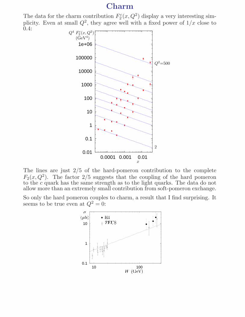
Charm

The data for the charm contribution F c2 (x,Q2) display a very interesting sim-

plicity. Even at small Q2, they agree well with a fixed power of 1/x close to0.4:

0.01

0.1

1

10

100

1000

10000

100000

1e+06

0.0001 0.001 0.01x

Q4 F c2 (x,Q2)

(GeV4)

Q2=500

2

The lines are just 2/5 of the hard-pomeron contribution to the completeF2(x,Q

2). The factor 2/5 suggests that the coupling of the hard pomeronto the c quark has the same strength as to the light quarks. The data do notallow more than an extremely small contribution from soft-pomeron exchange.

So only the hard pomeron couples to charm, a result that I find surprising. Itseems to be true even at Q2 = 0:

0.1

1

10

10 100W (GeV)

�(�b) H1ZEUS

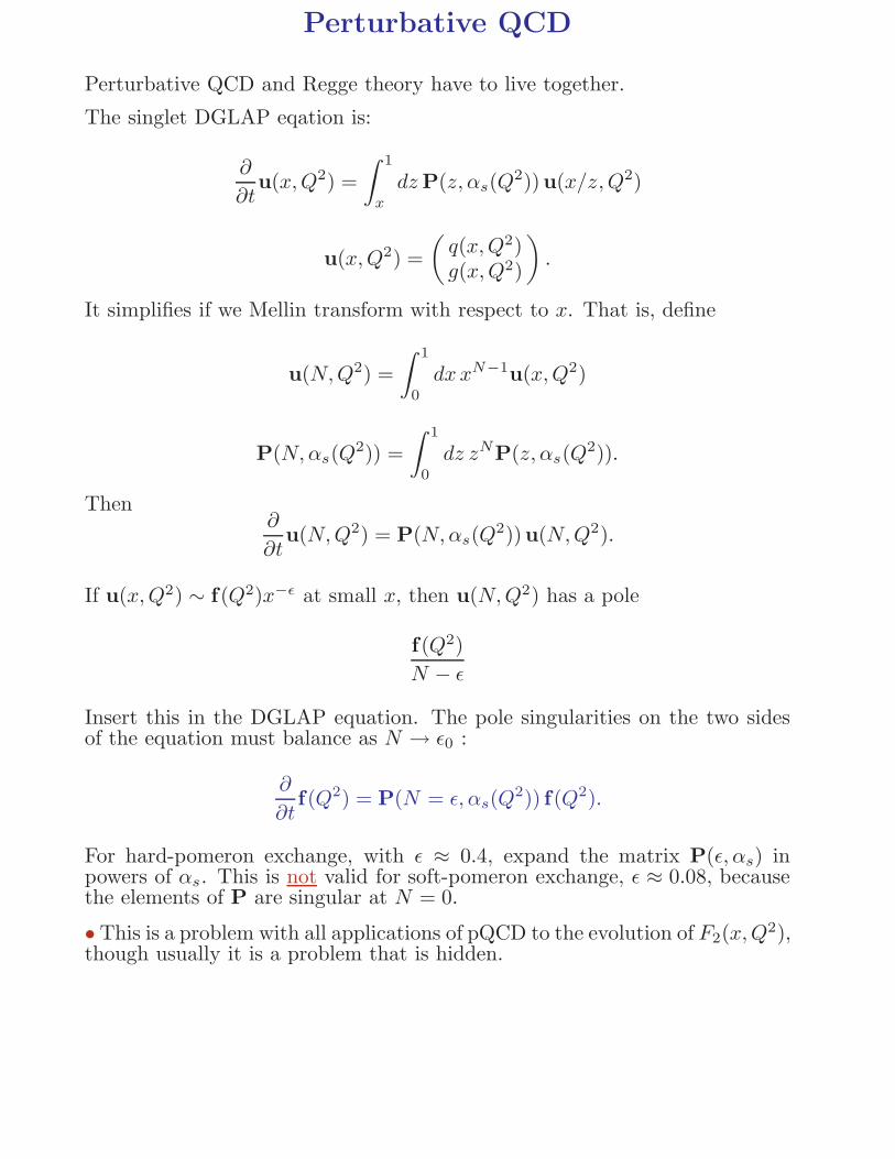
Perturbative QCD

Perturbative QCD and Regge theory have to live together.

The singlet DGLAP eqation is:

∂

∂tu(x,Q2) =

∫ 1

x

dzP(z, αs(Q2))u(x/z,Q2)

u(x,Q2) =

(

q(x,Q2)g(x,Q2)

)

.

It simplifies if we Mellin transform with respect to x. That is, define

u(N,Q2) =

∫ 1

0

dxxN−1u(x,Q2)

P(N,αs(Q2)) =

∫ 1

0

dz zNP(z, αs(Q2)).

Then∂

∂tu(N,Q2) = P(N,αs(Q

2))u(N,Q2).

If u(x,Q2) ∼ f(Q2)x−ǫ at small x, then u(N,Q2) has a pole

f(Q2)

N − ǫ

Insert this in the DGLAP equation. The pole singularities on the two sidesof the equation must balance as N → ǫ0 :

∂

∂tf(Q2) = P(N = ǫ, αs(Q

2)) f(Q2).

For hard-pomeron exchange, with ǫ ≈ 0.4, expand the matrix P(ǫ, αs) inpowers of αs. This is not valid for soft-pomeron exchange, ǫ ≈ 0.08, becausethe elements of P are singular at N = 0.

• This is a problem with all applications of pQCD to the evolution of F2(x,Q2),

though usually it is a problem that is hidden.

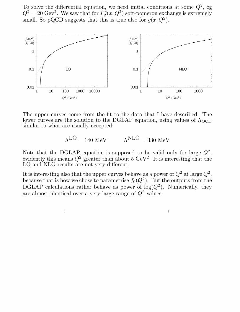
To solve the differential equation, we need initial conditions at some Q2, egQ2 = 20 Gev2. We saw that for F c

2 (x,Q2) soft-pomeron exchange is extremelysmall. So pQCD suggests that this is true also for g(x,Q2).

f0(Q2)

f0(20)

0.01

0.1

1

1 10 100 1000 10000

LO

Q2 (Gev2)

1

f0(Q2)

f0(20)

0.01

0.1

1

1 10 100 1000

NLO

Q2 (Gev2)

1

The upper curves come from the fit to the data that I have described. Thelower curves are the solution to the DGLAP equation, using values of ΛQCDsimilar to what are usually accepted:

ΛLO = 140 MeV ΛNLO = 330 MeV

Note that the DGLAP equation is supposed to be valid only for large Q2;evidently this means Q2 greater than about 5 GeV2. It is interesting that theLO and NLO results are not very different.

It is interesting also that the upper curves behave as a power of Q2 at largeQ2,because that is how we chose to parametrise f0(Q

2). But the outputs from theDGLAP calculations rather behave as power of log(Q2). Numerically, theyare almost identical over a very large range of Q2 values.

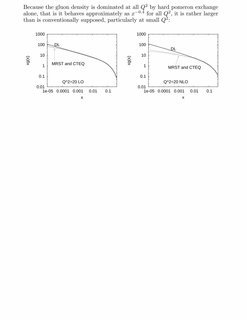
Because the gluon density is dominated at all Q2 by hard pomeron exchangealone, that is it behaves approximately as x−0.4 for all Q2, it is rather largerthan is conventionally supposed, particularly at small Q2:

0.01

0.1

1

10

100

1000

1e-05 0.0001 0.001 0.01 0.1

xg(x

)

x

Q^2=20 LO

DL

MRST and CTEQ

0.01

0.1

1

10

100

1000

1e-05 0.0001 0.001 0.01 0.1

xg(x

)

x

Q^2=20 NLO

DL

MRST and CTEQ

Regge factorisation

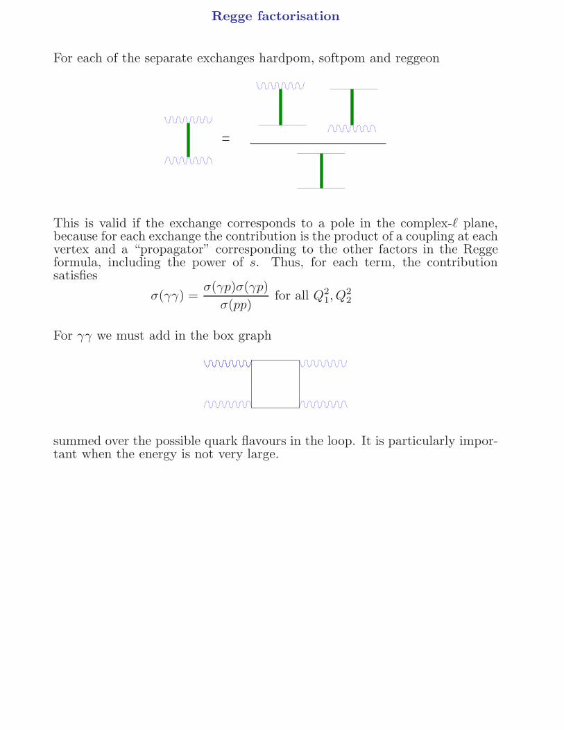
For each of the separate exchanges hardpom, softpom and reggeon

This is valid if the exchange corresponds to a pole in the complex-ℓ plane,because for each exchange the contribution is the product of a coupling at eachvertex and a “propagator” corresponding to the other factors in the Reggeformula, including the power of s. Thus, for each term, the contributionsatisfies

σ(γγ) =σ(γp)σ(γp)

σ(pp)for all Q2

1, Q22

For γγ we must add in the box graph

summed over the possible quark flavours in the loop. It is particularly impor-tant when the energy is not very large.

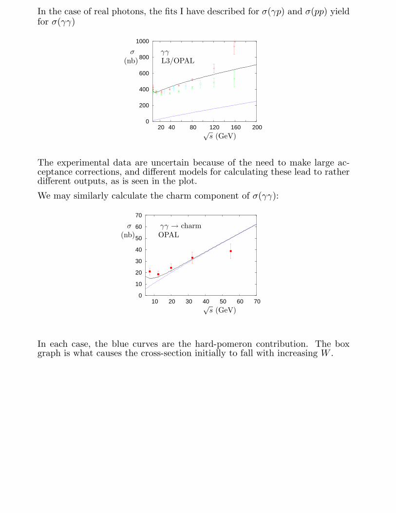
In the case of real photons, the fits I have described for σ(γp) and σ(pp) yieldfor σ(γγ)

0

200

400

600

800

1000

20 40 80 120 160 200√s (GeV)

σ γγ(nb) L3/OPAL

The experimental data are uncertain because of the need to make large ac-ceptance corrections, and different models for calculating these lead to ratherdifferent outputs, as is seen in the plot.

We may similarly calculate the charm component of σ(γγ):

0

10

20

30

40

50

60

70

10 20 30 40 50 60 70√s (GeV)

σ γγ → charm(nb) OPAL

In each case, the blue curves are the hard-pomeron contribution. The boxgraph is what causes the cross-section initially to fall with increasing W .

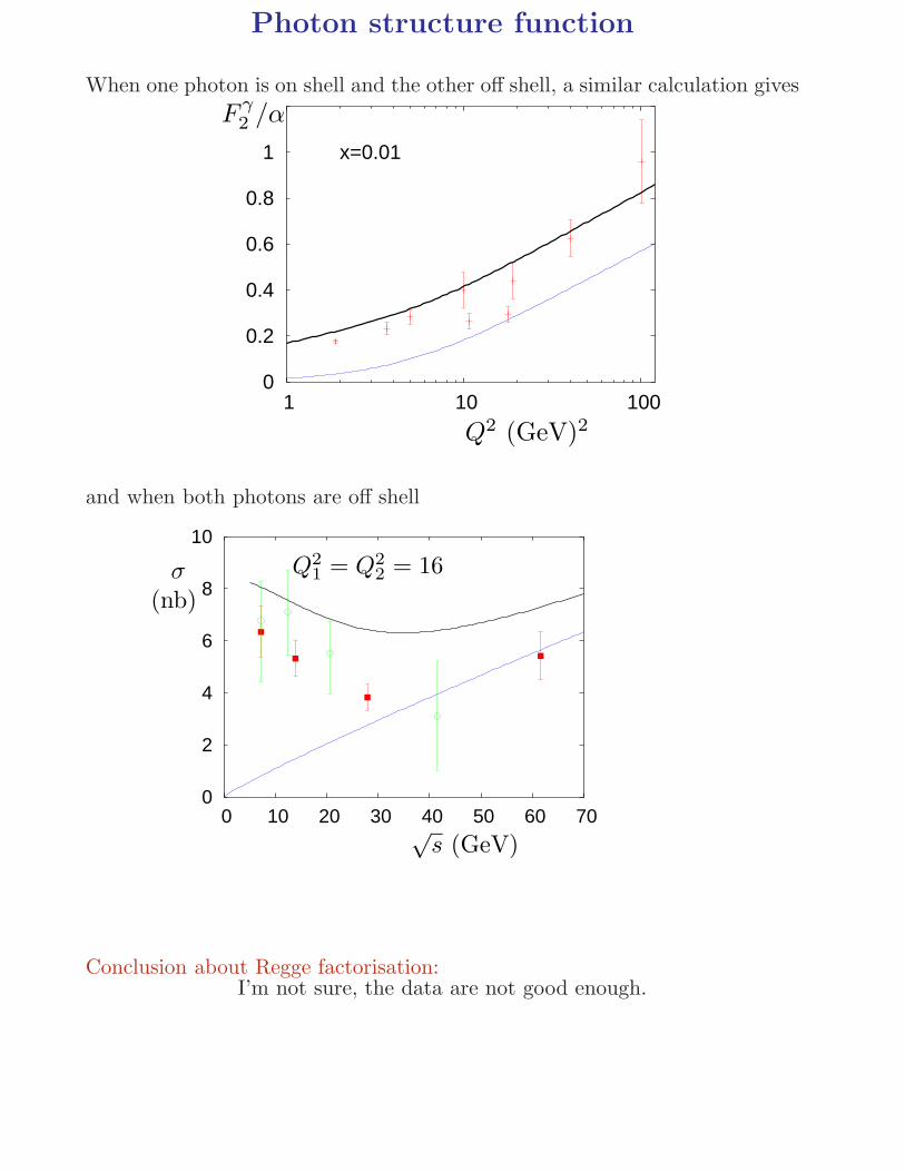
Photon structure function

When one photon is on shell and the other off shell, a similar calculation gives

0

0.2

0.4

0.6

0.8

1

1 10 100

x=0.01

Q2 (GeV)2

F γ2 /α

and when both photons are off shell

0

2

4

6

8

10

0 10 20 30 40 50 60 70√s (GeV)

σ(nb)

Q21 = Q2

2 = 16

Conclusion about Regge factorisation:I’m not sure, the data are not good enough.

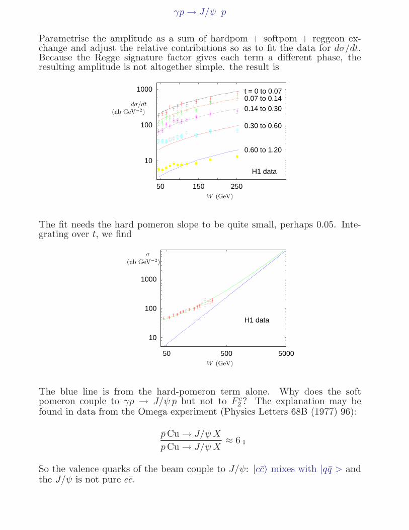
γp→ J/ψ p

Parametrise the amplitude as a sum of hardpom + softpom + reggeon ex-change and adjust the relative contributions so as to fit the data for dσ/dt.Because the Regge signature factor gives each term a different phase, theresulting amplitude is not altogether simple. the result is

10

100

1000

50 150 250

t = 0 to 0.070.07 to 0.140.14 to 0.30

0.30 to 0.60

0.60 to 1.20

H1 data

W (GeV)

dσ/dt(nb GeV−2)

1

The fit needs the hard pomeron slope to be quite small, perhaps 0.05. Inte-grating over t, we find

10

100

1000

50 500 5000

H1 data

W (GeV)

σ(nb GeV−2)

The blue line is from the hard-pomeron term alone. Why does the softpomeron couple to γp → J/ψ p but not to F c

2 ? The explanation may befound in data from the Omega experiment (Physics Letters 68B (1977) 96):

pCu → J/ψX

pCu → J/ψX≈ 6

So the valence quarks of the beam couple to J/ψ: |cc〉 mixes with |qq > andthe J/ψ is not pure cc.

Hard pomeron in hadron-hadron scattering?

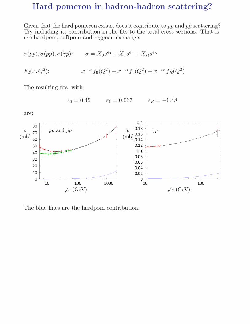
Given that the hard pomeron exists, does it contribute to pp and pp scattering?Try including its contribution in the fits to the total cross sections. That is,use hardpom, softpom and reggeon exchange:

σ(pp), σ(pp), σ(γp): σ = X0sǫ0 +X1s

ǫ1 +XRsǫR

F2(x,Q2): x−ǫ0f0(Q

2) + x−ǫ1f1(Q2) + x−ǫRfR(Q2)

The resulting fits, with

ǫ0 = 0.45 ǫ1 = 0.067 ǫR = −0.48

are:

0

10

20

30

40

50

60

70

80

10 100 1000√s (GeV)

σ pp and pp(mb)

00.020.040.060.080.1

0.120.140.160.180.2

10 100√s (GeV)

σ γp(mb)

The blue lines are the hardpom contribution.

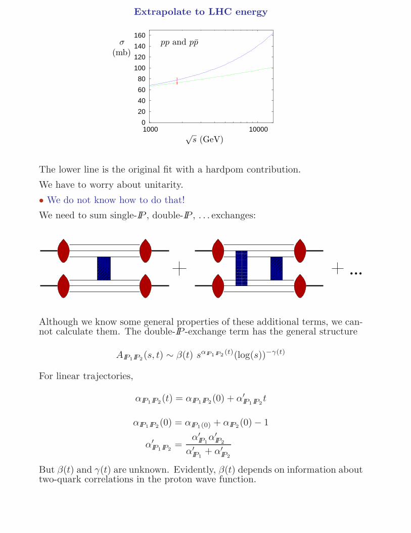
Extrapolate to LHC energy

0

20

40

60

80

100

120

140

160

1000 10000√s (GeV)

σ pp and pp(mb)

The lower line is the original fit with a hardpom contribution.

We have to worry about unitarity.

• We do not know how to do that!

We need to sum single-IP , double-IP , . . . exchanges:

��������������������������

��������������������������

������������������

������������������

������������������

������������������

...

Although we know some general properties of these additional terms, we can-not calculate them. The double-IP -exchange term has the general structure

AIP1IP2(s, t) ∼ β(t) sαIP1IP2

(t)(log(s))−γ(t)

For linear trajectories,

αIP1IP2(t) = αIP1IP2

(0) + α′

IP1IP2t

αIP1IP2(0) = αIP1(0) + αIP2

(0) − 1

α′

IP1IP2=

α′IP1α′

IP2

α′IP1

+ α′IP2

But β(t) and γ(t) are unknown. Evidently, β(t) depends on information abouttwo-quark correlations in the proton wave function.

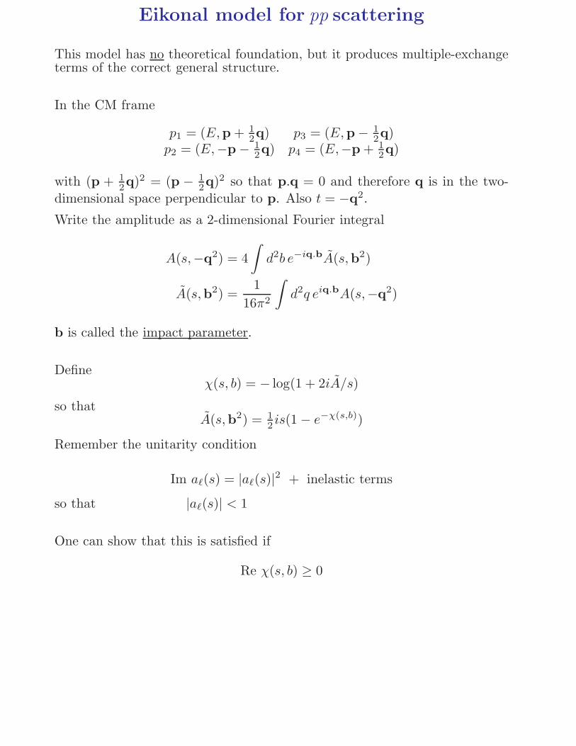
Eikonal model for pp scattering

This model has no theoretical foundation, but it produces multiple-exchangeterms of the correct general structure.

In the CM frame

p1 = (E,p + 12q) p3 = (E,p − 1

2q)p2 = (E,−p − 1

2q) p4 = (E,−p + 12q)

with (p + 12q)2 = (p − 1

2q)2 so that p.q = 0 and therefore q is in the two-

dimensional space perpendicular to p. Also t = −q2.

Write the amplitude as a 2-dimensional Fourier integral

A(s,−q2) = 4

∫

d2b e−iq.bA(s,b2)

A(s,b2) =1

16π2

∫

d2q eiq.bA(s,−q2)

b is called the impact parameter.

Defineχ(s, b) = − log(1 + 2iA/s)

so thatA(s,b2) = 1

2is(1 − e−χ(s,b))

Remember the unitarity condition

Im aℓ(s) = |aℓ(s)|2 + inelastic terms

so that |aℓ(s)| < 1

One can show that this is satisfied if

Re χ(s, b) ≥ 0

Expand the exponential as a power series:

A(s,−q2) = 2is

∫

d2b e−iq.b(1 − e−χ(s,b))

= 2is

∫

d2b e−iq.b(

χ− χ2

2!+χ3

3!. . .− (−χ)n

n!. . .

)

If first term is approximated by single-IP exchange, the second has the correctgeneral structure of double-IP exchange, etc. And one can then show that thenat very large s

σTot ∼ 4πα′ǫ0(log s)2

so the Froissart bound is satisfied.

But, although it has been widely used, this representation for the ampli-tude has little theoretical foundation. For example, the double-exchange termshould contain information about the two-quark correlation in the proton’swave function, but this is not present in the term χ2.

pp elastic scattering

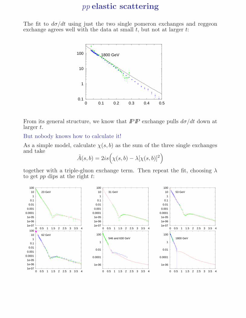
The fit to dσ/dt using just the two single pomeron exchanges and reggeonexchange agrees well with the data at small t, but not at larger t:

0.1

1

10

100

0 0.1 0.2 0.3 0.4 0.5

1800 GeV

From its general structure, we know that IPIP exchange pulls dσ/dt down atlarger t.

But nobody knows how to calculate it!

As a simple model, calculate χ(s, b) as the sum of the three single exchangesand take

A(s, b) = 2is(

χ(s, b) − λ[χ(s, b)]2)

together with a triple-gluon exchange term. Then repeat the fit, choosing λto get pp dips at the right t:

1e-07

1e-06

1e-05

0.0001

0.001

0.01

0.1

1

10

100

0 0.5 1 1.5 2 2.5 3 3.5 4

23 GeV

1e-07

1e-06

1e-05

0.0001

0.001

0.01

0.1

1

10

100

0 0.5 1 1.5 2 2.5 3 3.5 4

31 GeV

1e-07

1e-06

1e-05

0.0001

0.001

0.01

0.1

1

10

100

0 0.5 1 1.5 2 2.5 3 3.5 4

53 GeV

1e-07

1e-06

1e-05

0.0001

0.001

0.01

0.1

1

10

100

0 0.5 1 1.5 2 2.5 3 3.5 4

62 GeV

1e-06

0.0001

0.01

1

100

0 0.5 1 1.5 2 2.5 3 3.5 4

546 and 630 GeV

1e-06

0.0001

0.01

1

100

0 0.5 1 1.5 2 2.5 3 3.5 4

1800 GeV

Conclusion

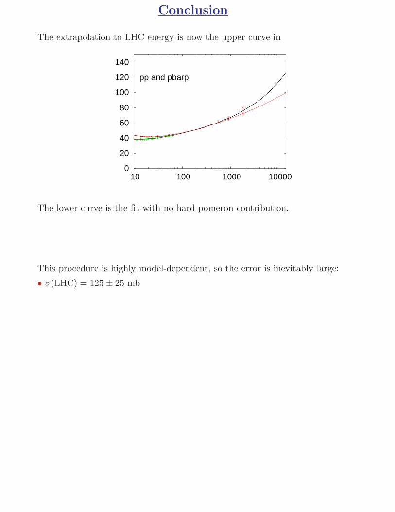
The extrapolation to LHC energy is now the upper curve in

0

20

40

60

80

100

120

140

10 100 1000 10000

pp and pbarp

The lower curve is the fit with no hard-pomeron contribution.

This procedure is highly model-dependent, so the error is inevitably large:

• σ(LHC) = 125 ± 25 mb