THE TIPPING POINT: VISUAL ESTIMATION OFTHE PHYSICAL STABILITY OF

THREE-DIMENSIONAL OBJECTS

BY STEVEN A. CHOLEWIAK

A dissertation submitted to the

Graduate School—New Brunswick

Rutgers, The State University of New Jersey

in partial fulfillment of the requirements

for the degree of

Doctor of Philosophy

Graduate Program in Psychology

Written under the direction of

Manish Singh

and approved by

New Brunswick, New Jersey

October, 2012

ABSTRACT OF THE DISSERTATION

The tipping point: Visual estimation of the physical

stability of three-dimensional objects

by STEVEN A. CHOLEWIAK

Dissertation Director:

Manish Singh

Vision research generally focuses on the currently visible surface properties of objects,

such as color, texture, luminance, orientation, and shape. In addition, however, ob-

servers can also visually predict the physical behavior of objects, which often requires

inferring the action of hidden forces, such as gravity and support relations. One of the

main conclusions from the naıve physics literature is that people often have inaccu-

rate physical intuitions; however, more recent research has shown that with dynamic

simulated displays, observers can correctly infer physical forces (e.g., timing hand move-

ments to catch a falling ball correctly takes into account Newtons laws of motion). One

ecologically important judgment about physical objects is whether they are physically

stable or not. This research project examines how people perceive physical stability and

addresses (1) How do visual estimates of stability compare to physical predictions? Can

observers track the influence of specific shape manipulations on object stability? (2)

Can observers match stability across objects with different shapes? How is the overall

stability of an object estimated? (3) Are visual estimates of object stability subject

to adaptation effects? Is stability a perceptual variable? The experimental findings

indicate that: (1) Observers are able to judge the stability of objects quite well and are

close to the physical predictions on average. They can track how changing a shape will

ii

affect the physical stability; however, the perceptual influence is slightly smaller than

physically predicted. (2) Observers can match the stabilities of objects with different

three-dimensional shapes – suggesting that object stability is a unitary dimension –

and their judgments of overall stability are strongly biased towards the minimum crit-

ical angle. (3) The majority of observers exhibited a stability adaptation aftereffect,

providing evidence in support of the claim that stability may be a perceptual variable.

iii

Acknowledgements

This work was supported by NSF Grants CCF-0541185 and DGE-0549115 (IGERT:

Interdisciplinary Training in Perceptual Science) and by NIH Grant EY021494.

Many thanks to Chris Kourtev for his technical assistance and the present and past

members of the Rutgers University Perceptual Science and Visual Cognition Laborato-

ries (including Kristina Denisova, Shalin Shah, Sung-Ho Kim, Bina Pastakia, Mehwish

Ajmal, Roy Jung, Stamatiki “Matina” Clapsis, Omer “Daglar” Tanrikulu, John Wilder,

Peter Pantelis, Vicky Froyen, and Seha Kim).

iv

Dedication

This research project would not have been possible without the support and guidance

of many of my fellow students and the faculty members in the Rutgers University

Psychology Department.

I wish to express my sincerest gratitude to my advisor, Dr. Manish Singh, whose in-

valuable support and guidance over the years has helped me “find my way” in academia

and to help strengthen my desire for knowledge. His insightful comments and construc-

tive criticisms of my projects have been instrumental in strengthening my research.

Thank you.

Deepest gratitude is also due to the members of the supervisory committee, Dr.

Jacob Feldman, Dr. Eileen Kowler, and Dr. Roland Fleming, without whose knowledge

and assistance – over the course of these past few years –, this research would not have

been successful.

I also wish to express my gratitude to my family and friends, especially my best

friend (and wife!) Sara and parents Roger and Linda, who have put up with endless

discussions about “whether or not this beer glass will fall”, “How might I perceptually

represent this [or that]?”, and “What’s the functional form for this surface? I want to

calculate its properties analytically...”. You are all saints.

v

Table of Contents

Abstract . . . . . . . . . . . . . . . . . . . . . . . . . . . . . . . . . . . . . . . . ii

Acknowledgements . . . . . . . . . . . . . . . . . . . . . . . . . . . . . . . . . iv

Dedication . . . . . . . . . . . . . . . . . . . . . . . . . . . . . . . . . . . . . . . v

1. Introduction . . . . . . . . . . . . . . . . . . . . . . . . . . . . . . . . . . . 1

1.1. Naıve physics . . . . . . . . . . . . . . . . . . . . . . . . . . . . . . . . . 2

1.2. Perceptual inference of motion and forces from static images . . . . . . . 9

1.3. Perception of Physical Stability . . . . . . . . . . . . . . . . . . . . . . . 16

1.4. Research Questions . . . . . . . . . . . . . . . . . . . . . . . . . . . . . . 23

2. Perception of physical stability of 3D objects: The role of aspect ratio

and parts . . . . . . . . . . . . . . . . . . . . . . . . . . . . . . . . . . . . . . . 25

2.1. Introduction . . . . . . . . . . . . . . . . . . . . . . . . . . . . . . . . . . 25

2.2. Experiment 1A: Perception of Object Stability . . . . . . . . . . . . . . 31

2.2.1. Methods . . . . . . . . . . . . . . . . . . . . . . . . . . . . . . . . 32

Observers . . . . . . . . . . . . . . . . . . . . . . . . . . . . . . . 32

Apparatus . . . . . . . . . . . . . . . . . . . . . . . . . . . . . . . 32

Stimuli and Design . . . . . . . . . . . . . . . . . . . . . . . . . . 32

2.2.2. Results . . . . . . . . . . . . . . . . . . . . . . . . . . . . . . . . 34

2.2.3. Discussion . . . . . . . . . . . . . . . . . . . . . . . . . . . . . . . 38

2.3. Experiment 1B: Perception of Center of Mass . . . . . . . . . . . . . . . 39

2.3.1. Methods . . . . . . . . . . . . . . . . . . . . . . . . . . . . . . . . 40

Observers . . . . . . . . . . . . . . . . . . . . . . . . . . . . . . . 40

Apparatus . . . . . . . . . . . . . . . . . . . . . . . . . . . . . . . 40

Stimuli and Design . . . . . . . . . . . . . . . . . . . . . . . . . . 40

vi

2.3.2. Results . . . . . . . . . . . . . . . . . . . . . . . . . . . . . . . . 42

2.3.3. Discussion . . . . . . . . . . . . . . . . . . . . . . . . . . . . . . . 47

2.4. Experiment 2: The Role of Parts . . . . . . . . . . . . . . . . . . . . . . 48

2.4.1. Methods . . . . . . . . . . . . . . . . . . . . . . . . . . . . . . . . 49

Observers . . . . . . . . . . . . . . . . . . . . . . . . . . . . . . . 49

Apparatus . . . . . . . . . . . . . . . . . . . . . . . . . . . . . . . 49

Stimuli and Design . . . . . . . . . . . . . . . . . . . . . . . . . . 49

2.4.2. Results . . . . . . . . . . . . . . . . . . . . . . . . . . . . . . . . 50

2.5. Conclusion . . . . . . . . . . . . . . . . . . . . . . . . . . . . . . . . . . 52

3. Perception of the physical stability of asymmetrical three-dimensional

objects . . . . . . . . . . . . . . . . . . . . . . . . . . . . . . . . . . . . . . . . . 55

3.1. Introduction . . . . . . . . . . . . . . . . . . . . . . . . . . . . . . . . . . 55

3.2. Experiment 1: Measuring Critical Angle in Different Directions . . . . . 58

3.2.1. Methods . . . . . . . . . . . . . . . . . . . . . . . . . . . . . . . . 59

Observers . . . . . . . . . . . . . . . . . . . . . . . . . . . . . . . 59

Apparatus . . . . . . . . . . . . . . . . . . . . . . . . . . . . . . . 59

Stimuli and Design . . . . . . . . . . . . . . . . . . . . . . . . . . 60

Procedure . . . . . . . . . . . . . . . . . . . . . . . . . . . . . . . 61

3.2.2. Results . . . . . . . . . . . . . . . . . . . . . . . . . . . . . . . . 61

3.2.3. Discussion . . . . . . . . . . . . . . . . . . . . . . . . . . . . . . . 62

3.3. Experiment 2: Matching Overall Stability . . . . . . . . . . . . . . . . . 63

3.3.1. Motivation . . . . . . . . . . . . . . . . . . . . . . . . . . . . . . 63

3.3.2. Methods . . . . . . . . . . . . . . . . . . . . . . . . . . . . . . . . 65

Observers . . . . . . . . . . . . . . . . . . . . . . . . . . . . . . . 65

Stimuli and Design . . . . . . . . . . . . . . . . . . . . . . . . . . 65

Procedure . . . . . . . . . . . . . . . . . . . . . . . . . . . . . . . 66

3.3.3. Results . . . . . . . . . . . . . . . . . . . . . . . . . . . . . . . . 67

3.3.4. Discussion . . . . . . . . . . . . . . . . . . . . . . . . . . . . . . . 70

vii

3.4. Experiment 3: Matching Overall Stability in Different Directions . . . . 70

3.4.1. Motivation . . . . . . . . . . . . . . . . . . . . . . . . . . . . . . 70

3.4.2. Methods . . . . . . . . . . . . . . . . . . . . . . . . . . . . . . . . 71

Observers . . . . . . . . . . . . . . . . . . . . . . . . . . . . . . . 71

Stimuli and Design . . . . . . . . . . . . . . . . . . . . . . . . . . 71

Procedure . . . . . . . . . . . . . . . . . . . . . . . . . . . . . . . 72

3.4.3. Results . . . . . . . . . . . . . . . . . . . . . . . . . . . . . . . . 72

3.4.4. Discussion . . . . . . . . . . . . . . . . . . . . . . . . . . . . . . . 72

3.5. Conclusion . . . . . . . . . . . . . . . . . . . . . . . . . . . . . . . . . . 74

4. Visual adaptation to the physical stability of objects . . . . . . . . . . 76

4.1. Introduction . . . . . . . . . . . . . . . . . . . . . . . . . . . . . . . . . . 76

4.2. Experiment 1: 2D Curvature Probe . . . . . . . . . . . . . . . . . . . . . 78

4.2.1. Methods . . . . . . . . . . . . . . . . . . . . . . . . . . . . . . . . 78

Observers . . . . . . . . . . . . . . . . . . . . . . . . . . . . . . . 78

Apparatus . . . . . . . . . . . . . . . . . . . . . . . . . . . . . . . 78

Adaptation Stimuli . . . . . . . . . . . . . . . . . . . . . . . . . . 79

Test Stimuli . . . . . . . . . . . . . . . . . . . . . . . . . . . . . . 80

Design . . . . . . . . . . . . . . . . . . . . . . . . . . . . . . . . . 81

4.2.2. Results . . . . . . . . . . . . . . . . . . . . . . . . . . . . . . . . 83

4.2.3. Discussion . . . . . . . . . . . . . . . . . . . . . . . . . . . . . . . 83

4.3. Experiment 2: 2D Shift Probe . . . . . . . . . . . . . . . . . . . . . . . . 84

4.3.1. Methods . . . . . . . . . . . . . . . . . . . . . . . . . . . . . . . . 85

Observers . . . . . . . . . . . . . . . . . . . . . . . . . . . . . . . 85

Apparatus . . . . . . . . . . . . . . . . . . . . . . . . . . . . . . . 85

Adaptation Stimuli . . . . . . . . . . . . . . . . . . . . . . . . . . 85

Test Stimuli . . . . . . . . . . . . . . . . . . . . . . . . . . . . . . 86

Design . . . . . . . . . . . . . . . . . . . . . . . . . . . . . . . . . 87

4.3.2. Results . . . . . . . . . . . . . . . . . . . . . . . . . . . . . . . . 88

viii

4.3.3. Discussion . . . . . . . . . . . . . . . . . . . . . . . . . . . . . . . 89

4.4. Experiment 3: 3D Curvature Probe . . . . . . . . . . . . . . . . . . . . . 89

4.4.1. Methods . . . . . . . . . . . . . . . . . . . . . . . . . . . . . . . . 90

Observers . . . . . . . . . . . . . . . . . . . . . . . . . . . . . . . 90

Apparatus . . . . . . . . . . . . . . . . . . . . . . . . . . . . . . . 90

Adaptation Stimuli . . . . . . . . . . . . . . . . . . . . . . . . . . 90

Test Stimuli . . . . . . . . . . . . . . . . . . . . . . . . . . . . . . 91

Design . . . . . . . . . . . . . . . . . . . . . . . . . . . . . . . . . 92

4.4.2. Results . . . . . . . . . . . . . . . . . . . . . . . . . . . . . . . . 93

4.4.3. Discussion . . . . . . . . . . . . . . . . . . . . . . . . . . . . . . . 94

4.5. Experiment 4: 3D Shift Probe . . . . . . . . . . . . . . . . . . . . . . . . 94

4.5.1. Methods . . . . . . . . . . . . . . . . . . . . . . . . . . . . . . . . 95

Observers . . . . . . . . . . . . . . . . . . . . . . . . . . . . . . . 95

Apparatus . . . . . . . . . . . . . . . . . . . . . . . . . . . . . . . 95

Adaptation Stimuli . . . . . . . . . . . . . . . . . . . . . . . . . . 95

Test Stimuli . . . . . . . . . . . . . . . . . . . . . . . . . . . . . . 95

Design . . . . . . . . . . . . . . . . . . . . . . . . . . . . . . . . . 96

4.5.2. Results . . . . . . . . . . . . . . . . . . . . . . . . . . . . . . . . 96

4.6. Conclusion . . . . . . . . . . . . . . . . . . . . . . . . . . . . . . . . . . 97

5. Conclusion . . . . . . . . . . . . . . . . . . . . . . . . . . . . . . . . . . . . 100

References . . . . . . . . . . . . . . . . . . . . . . . . . . . . . . . . . . . . . . . 104

ix

1

Chapter 1

Introduction

Vision research generally focuses on currently visible surface properties, such as color,

texture, luminance, orientation, and shape. Representing these properties provides a

useful visual description of a scene and the objects therein: what the various objects

are, where they are located relative to each other, and relative to the observer. There

are some notable exceptions to the focus on visible surface properties, where researchers

investigate the perceptual representation of surfaces (or portions of surfaces) that are

not currently visible – that is, have no counterpart in the retinal images – as well as

predicting where objects will be in the near future. Both modal completion, where

observers perceive an illusory contour occluding another shape (e.g., Kanizsa triangle

& illusory contours), and amodal completion, where a complete shape is perceived even

though contours are partly occluded, involve the inference of contours and surfaces that

are not visible (Anderson, Singh, & Fleming, 2002; Singh, 2004). Similarly, observers

can visually extrapolate the trajectory of a moving object (Becker & Fuchs, 1985; Pavel,

Cunningham, & Stone, 1992; Verghese & McKee, 2002), and predict where an object

that disappears behind an occluder is likely to re-emerge from (Scholl & Pylyshyn,

1999; Graf, Warren, & Maloney, 1995; Shah, Fulvio, & Singh, 2012).

However, these representational processes do not involve the inference of physical

forces acting upon the objects. This inference of forces is critical in predicting the

physical behavior of objects because the application of forces can lead to translation,

rotation, and acceleration, or non-rigid deformation of real-world objects. Therefore,

although it is important for the visual system to represent the shape and other surface

properties of objects as they currently exist, it is also important to be able to also infer

forces and predict the behavior of physical objects in the immediate future – e.g., for

2

the purpose of guiding motor action.

The inference of forces is crucial for the manipulation of physical objects; without it,

one could not interact with the world. Mounting evidence supports an internal, mental

model of physics that is applied during object interaction. For example, observers are

sensitive to the effects of gravity (I. K. Kim & Spelke, 1992; Friedman, 2002; McIntyre,

Zago, Berthoz, & Lacquaniti, 2001). The inference of forces also allows for the prediction

of how colliding objects will interact (Cooper, Birnbaum, & Brand, 1995; Newman,

Choi, Wynn, & Scholl, 2008) and how frictional forces will affect the movement of

objects (by decelerating their motion). Visual surface properties can provide some of

the necessary information for inferring forces, such as texture providing information

about friction, but visible surface properties alone cannot be used to predict object

behavior. The brain must also have an internal model of how physical forces act and

how they influence the behavior of objects.

A growing body of research has shown that individuals use models of forces, similar

to the classical “Newton’s Laws”, when predicting object behavior and interactions

with other objects. The visual system uses inferred – unseen – forces to plan motor

actions (e.g., predicting the trajectory of an arrow or calculating the contact angle for

a billiard cue stick in order to strike a ball to sink another) and to assist in decision

making. The area of psychology that investigates how humans infer information about

forces and use it in the service of future action is known as “naıve physics”. This

research project’s goal is to study how we judge physical attributes of objects and to

determine if our judgments of stability conform to the beliefs of the traditional “naıve

physics” literature, which had largely concluded that people apply inaccurate physical

models, or whether our inference of forces allows us to make judgments in a more

physically-correct manner in more perceptual contexts.

1.1 Naıve physics

Humans are constantly interacting with the world around them, observing the behavior

and interaction of objects in the environment and using these observations to inform

3

future decisions and motor actions. The study of naıve physics – how people represent

and use models of physical forces and causes of motion – has focused on answering

the question of whether or not humans embody physically-correct representations of

physics and if they can accurately predict the physical behavior of objects. In order

to make physically-accurate predictions, humans must have a system that embodies a

model of physics.

In the “real world”, the physical behavior of objects of the environment can be

physically defined using statics and dynamics (branches of classical mechanics) and,

in many cases – where objects move at a constant velocity or are only affected by

the force of gravity – the physical behavior of objects can simply be described using

Newton’s laws of motion. For people to accurately predict object motion and future

behavior, their internal models must use the object’s velocity and acceleration to infer

the physical forces acting upon the object (e.g., as described by Newton’s laws). An

important question is whether these internal models are consistent with Newton’s laws

and whether or not people use physically-derived models of motion and object behavior.

The naıve physics literature has sought to determine how well people use the behavior

of moving objects to predict how they will behave in the near-future. Do they use a

physically-accurate dynamic model – using correctly inferred forces – or a simpler model

that, while not always physically-correct, can provide reasonably accurate answers most

of the time (e.g., a model that utilizes heuristics)?

A representational model of physics would allow people to observe object behavior

and estimate the forces acting upon the object, so that the visual system can predict

the object’s future location. Naıve physics research has focused on describing percep-

tual and cognitive models of inferred forces and how people use them – correctly and

incorrectly – to predict object motion. And, as with most representations, these motion

predictions are constantly, unconsciously updated, allowing us to use prior perceptual

information with a representation of the the physical world in the service of future

action (e.g., to catch a falling ball).

Do people use physically-accurate models when representing object motion? There

is evidence that people can do this for the simpler, less complex situations. Human

4

observers can easily identify the position of objects and track/extrapolate the motion

of objects that move at constant velocity (i.e., motion that conforms to Newton’s 1st

law) (Pavel et al., 1992). There is also evidence that people use a representation of

implied motion when observing object behavior and recalling its location/orientation

some time in the future.

Representational momentum (RM) is a subarea of naıve physics that has found

that representations of object motion interfere with observers’ memories of the object’s

location and/or orientation (Freyd, 1983; Freyd & Finke, 1984; Freyd & Jones, 1994).

Freyd (1983) suggested that observers generate a dynamic mental representation of an

object’s motion when shown a series of images implying object motion and that this

dynamic representation can continue to change, based upon the object’s prior motion,

interfering with “static” memories of the last seen state.

Freyd and Finke (1984) showed observers a rectangle spinning counter-clockwise in

a series of images, then presented a frame that was either the same or different from

the last image shown and asked, “Is this image the same or different from the last one

shown?” (see Fig. 1.1). Observers had more difficulty identifying frames that continued

the motion as different from the last presented frame compared to images that showed

motion in the opposite direction, which were readily identified as different. Observers

appeared to misjudge the orientation of the last frame when presented with a sequence

that implies motion. Freyd and Finke (1984) posited that observers generate a repre-

sentation of the motion and that this representation was interfering with their memories

of the last frame in the motion sequence. They found that this RM interference requires

coherent motion – that is, a series of images that continue motion in a single direction

– otherwise, no dynamic mental representation of the object’s motion is generated and

people can readily identify images that are different. Because observers are automati-

cally computing the predicted trajectory and using constant velocity information, they

cannot help but be influenced by that representation.

People are able to use constant velocity information, but how do they integrate

this information over time, for example with accelerating objects? As predicted from

a computational complexity argument, observers have more difficulty when predicting

5

Figure 1.1: Sequence of test images demonstrating representational momentum (Freyd& Finke, 1984).

motion affected by the acceleration due to a net force (i.e., motion that conforms to

Newton’s 2nd law). Extrapolating motion becomes more difficult for people when the

object(s) undergo acceleration due to an implied force, even when the acceleration is a

constant centripetal acceleration (e.g., a ball on a string being swung in a circle).

If observers always used position, velocity, and linear acceleration in a physically-

consistent, mathematically-derived manner when predicting object motion, then they

should be able to predict how forces acting upon an object will affect an object’s

trajectory. In the gross majority of circumstances, we are able to track movement

and account for changing direction – whether due to internal or external forces. And

this fact is reflected in evidence that people utilize a physically accurate model that

incorporates acceleration due to gravitational forces.

All objects with mass on Earth have a gravitational force acting upon their bodies

and it appears as though humans develop a representation at an early age (I. K. Kim

& Spelke, 1992; Friedman, 2002) and account for gravity when trying to grab a falling

object (McIntyre et al., 2001; Zago & Lacquaniti, 2005). Real-time motor tasks, such

as predicting time-to-impact (TTI) in order to catch an object, require relatively quick

responses and observers often do not have much of time – on the order of a few hundred

milliseconds – to compute a detailed prediction of the trajectory. However, it appears

6

as though these observers use a physically-accurate model of gravity when predicting

the TTI of objects moving under the force of a constant gravitational field.

As McIntyre et al. (2001) and Zago and Lacquaniti (2005) demonstrated, although

people sometimes use acceleration correctly, they do not always correctly infer how

forces will affect a moving object’s velocity and acceleration. White (1983) provided

additional evidence that observers have difficulty understanding how forces affect the

trajectory of moving object. Specifically, White (1983) showed that undergraduate

students had difficulty describing force impulses necessary for a spaceship to fly in

a circular path (i.e., centripetal acceleration), a square path (i.e., using impulses to

slow the ship and turn at each corner), and in any trajectory that required multiple

temporally-separated force impulses (see Fig. 1.2). When people are required to predict

motion affected by an external force, they have difficulties using a physically-correct

model and often fail to correctly incorporate the temporal component.

One possibility is that higher-level cognitive intuitions lead a person to use a physically-

incorrect model. This will often occur when observers are asked to answer paper-and-

pencil questions (with static diagrams), or solve a specific physical problem where they

must predict the trajectory of an object dropped or propelled.

The curved trajectories of objects moved using “external” forces are often mistak-

enly believed to continue their trajectories once those forces are removed (McCloskey,

1983a). These are often every-day situations where an accurate mental model (such as

the gravitational force model described earlier) would be ecologically important. For

example, a ball on a string is illustrated as being swung in a circle and observers are

asked what trajectory the ball will take if the string breaks. The majority of observers

describe the resulting trajectory as continuing in a circle, as if centripetal force contin-

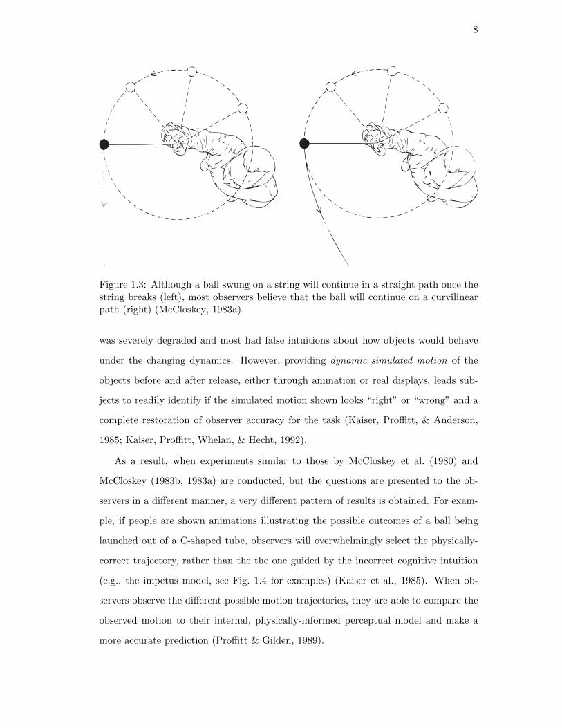
ued to act upon the ball after it has been released (see Fig. 1.3).

Research into how people apply implied forces to motion has shown that observers

will use the wrong physical model – as opposed to one simply missing higher-order terms

that incorporate acceleration – to guide their intuitions/judgments about an object’s

future motion (McCloskey, Caramazza, & Green, 1980; McCloskey, 1983b, 1983a).

The wrong model that most people use, in this case, is this impetus theory – where

7

(a) Responses for forces for circular path

(b) Responses for forces for square path

Figure 1.2: Examples of White (1983)’s paper and pencil task questions where observersfail to demonstrate a working knowledge of how external forces can affect the trajectoryof an object. Percentages of responses for each option are in parentheses. In (a),observers were asked “Can you draw a picture and explain how you would get yourspaceship to fly in a circular path?”. Note that the majority of responses were incorrect.In (b), observers were asked “Can you draw a description of how you would get yourspaceship to fly in a square path?” and most observers could not correctly determinethe appropriate forces.

objects are believed to embody an internal force that propels them, which gradually

dissipates over time – that makes very different predictions for an object’s trajectory

than Newtonian motion. The majority of the naıve physics research investigating how

people perceive implied forces has focused on tasks where the observers have had to

extrapolate future motion based upon their intuitions of the physical forces acting upon

the object(s) (McCloskey et al., 1980; McCloskey, 1983b, 1983a; McCloskey & Kohl,

1983; McCloskey, Washburn, & Felch, 1983).

A common feature of these studies was that they were all tasks where observers

made a decision about the motion of a system (i.e., a bomb dropping from a plane or

the trajectory of an object tossed by a catapult), where subjects were shown pictures

or given descriptions from which they had to make future predictions. When observers

were asked how the object would continue its motion, their performance on these tasks

8

Figure 1.3: Although a ball swung on a string will continue in a straight path once thestring breaks (left), most observers believe that the ball will continue on a curvilinearpath (right) (McCloskey, 1983a).

was severely degraded and most had false intuitions about how objects would behave

under the changing dynamics. However, providing dynamic simulated motion of the

objects before and after release, either through animation or real displays, leads sub-

jects to readily identify if the simulated motion shown looks “right” or “wrong” and a

complete restoration of observer accuracy for the task (Kaiser, Proffitt, & Anderson,

1985; Kaiser, Proffitt, Whelan, & Hecht, 1992).

As a result, when experiments similar to those by McCloskey et al. (1980) and

McCloskey (1983b, 1983a) are conducted, but the questions are presented to the ob-

servers in a different manner, a very different pattern of results is obtained. For exam-

ple, if people are shown animations illustrating the possible outcomes of a ball being

launched out of a C-shaped tube, observers will overwhelmingly select the physically-

correct trajectory, rather than the the one guided by the incorrect cognitive intuition

(e.g., the impetus model, see Fig. 1.4 for examples) (Kaiser et al., 1985). When ob-

servers observe the different possible motion trajectories, they are able to compare the

observed motion to their internal, physically-informed perceptual model and make a

more accurate prediction (Proffitt & Gilden, 1989).

9

Figure 1.4: Example possible trajectories for a ball exiting a C-shaped tube (Kaiseret al., 1985). Note that providing animated displays illustrating the different possibleoutcomes leads to observers choosing the correct trajectory (3) while paper-and-penciltasks often lead to incorrect responses.

To answer the question, “How well can people infer motion and forces acting upon

objects in motion?”, we can say that although humans often effectively use motion

to extrapolate an object’s location at a future point in time, it is not necessarily an

easy task. More often than not, people appear to revert to simplified physical models

that rely on the velocity of the object to describe its motion and fail to take into

account acceleration. This seems to reflect a competition between high-level intuitions

and perceptual judgments when viewing dynamic simulated motion sequences because

people’s performance depends on the way in which the question is posed: whether they

are asked to report a high-level intuition, or make a perceptual judgment about whether

a simulated scene looks “right.”

1.2 Perceptual inference of motion and forces from static images

All of the previously discussed naıve physics experiments involve inferring forces from

dynamic scenes (i.e., scenarios that include a motion component). Each experiment

involved the inference of forces acting upon a moving object and using prior motion

information to make a judgment about where the object will go. However, continuous

10

(a) Frame n (b) Frame n+1

Figure 1.5: Before (a) and after (b) frames of an action sequence from Freyd (1983),where a person was shown jumping off a small ledge.

smooth movement/animation is not necessary for people to perceive motion. People

perceive motion with as few as two frames of animation (Wertheimer, 1912; Korte,

1915).

Apparent motion in photographic sequences can give such a strong perception of

motion that people readily generate a dynamic mental representation of the motion,

which interferes with their memory of the scene and, subsequently, change detection.

An example from Freyd (1983) used two frames from a video of a person jumping off a

ledge (see Fig. 1.5). When observers were shown a future frame from the video where a

person’s body has translated down due to the force of gravity, observers had difficulty

detecting the change and took longer to respond that the image was different and that

the body had moved, consistent with an RM account.

There are many cases where forces and motion are inferred from a single static

image, where we see implied motion without additional temporal frames. For example,

when shown an image of a person in mid-air with his legs bent back and his body over

the precipice of a ledge, people will usually assume that the person had jumped off the

edge (e.g., Fig. 1.5b alone). That is, observers do not simply describe the static image

of the person’s body as floating in mid-air, instead they perceive him as in motion and

falling. Adding cues, such as blur (Gibson, 1954; Geilser, 1999) or speedlines (Burr &

Ross, 2002), strengthen the percept of motion and may lead observers to apply physical

11

(a) Leftward/Rightward (b) Outward/Inward

Figure 1.6: Example stimuli from Winawer et al., illustrating photographs with impliedleftward and rightward motion (a) and outward and inward motion (b).

models when judging the person’s past, present, and future states.

These dynamic motion representations have been shown to adapt observers to future

motion in the direction of the implied motion. Winawer, Huk, and Boroditsky (2008)

showed observers a series of implied motion photographs with either leftward, rightward,

inward, or outward motion (e.g., see Fig. 1.6) and then presented them with a moving

dot field and asked observers to respond what direction the dots moved. They found

that observers became adapted to the direction of motion present in the implied motion

photographs and responded that null motion stimuli – with no net motion in any given

direction – moved in the opposite direction (a motion aftereffect). Therefore, when we

see a static image of an object in motion, we may create a dynamic representation that

leads us to expect motion in the direction of the implied motion.

Research has also shown that implied motion in photographs tune observers’ per-

ceptual systems to expect motion in the direction of the motion and leads to enhanced

12

(a) Implied Motion (b) Non-implied Motion

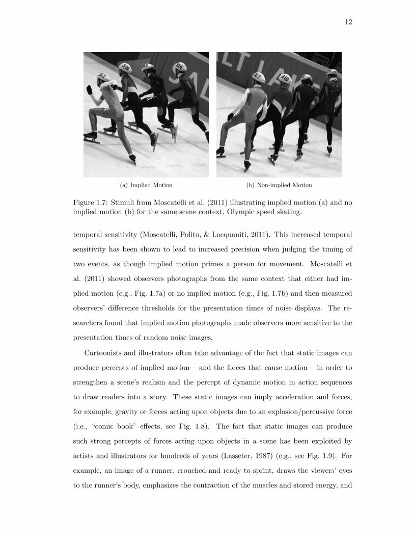
Figure 1.7: Stimuli from Moscatelli et al. (2011) illustrating implied motion (a) and noimplied motion (b) for the same scene context, Olympic speed skating.

temporal sensitivity (Moscatelli, Polito, & Lacquaniti, 2011). This increased temporal

sensitivity has been shown to lead to increased precision when judging the timing of

two events, as though implied motion primes a person for movement. Moscatelli et

al. (2011) showed observers photographs from the same context that either had im-

plied motion (e.g., Fig. 1.7a) or no implied motion (e.g., Fig. 1.7b) and then measured

observers’ difference thresholds for the presentation times of noise displays. The re-

searchers found that implied motion photographs made observers more sensitive to the

presentation times of random noise images.

Cartoonists and illustrators often take advantage of the fact that static images can

produce percepts of implied motion – and the forces that cause motion – in order to

strengthen a scene’s realism and the percept of dynamic motion in action sequences

to draw readers into a story. These static images can imply acceleration and forces,

for example, gravity or forces acting upon objects due to an explosion/percussive force

(i.e., “comic book” effects, see Fig. 1.8). The fact that static images can produce

such strong percepts of forces acting upon objects in a scene has been exploited by

artists and illustrators for hundreds of years (Lasseter, 1987) (e.g., see Fig. 1.9). For

example, an image of a runner, crouched and ready to sprint, draws the viewers’ eyes

to the runner’s body, emphasizes the contraction of the muscles and stored energy, and

13

Figure 1.8: Panels from Action Comics, No. 1 (p.5), illustrating how static images canconvey supportive forces (center panel), motion (right panel), and percussive forces.

primes the viewers to anticipate an explosive force from the runner’s legs.

Still images only provide a snapshot of a dynamic scene at any given moment in

time and cannot provide information about an object’s previous states that would cue

the observer to future motion (Freyd & Finke, 1984; Freyd & Jones, 1994). Given

the lack of temporal cues that multiple frames of video/animation can provide and the

relatively small amount of information that can lead to such a strong percept of motion

in a static image, the question is posed: How do we perceptually infer forces from static

images?

Experiments by Freyd, Pantzer, and Cheng (1988) demonstrated that static images

can convey an implied force structure and that this force information may be encoded

in the representation of the scene. Observers were first presented with static scenes

where a hanging plant had supportive forces – either a pedestal/stand that supported

the object from the bottom or a hook that supported it from the top – then an image of

the plant unsupported and then the plant above, below, or in the same position. Freyd

et al. (1988) found that observers had greater difficulty when making same/different

judgments if the test image of the plant was below its previous location (as opposed to

above), consistent with motion due to a gravitational force. This result suggests that

people inferred the force of gravity acting upon the plant and this inferred force and

14

(a) (b) (c)

Figure 1.9: Examples of classical artwork illustrating static images capturing dynamicscenes:(a) Bonaparte Crossing the Frand Saint-Bernard Pass, May 20, 1800, Jacques LouisDavid(b) Inset from Capture of the city and citadel of Gand in six days, 1678, Charles LeBrun(c) Hercules and the Hydra and Hercules and Anteo, Antonio del Pollaiolo

it’s implied motion interfered with observers’ memory of the plant’s last location.

Roncato and Rumiati (1986) found that although people can perceive the forces

acting upon suspended objects in static images, their judgments often do not match

physical reality when asked to make a judgment of an object’s orientation in the future,

after the forces have acted upon it. They showed observers scenes where a bar was

suspended by a wire and supported by props from the underside (see Fig. 1.10). The

bars were suspended at different points along their axes, including at the center of

gravity. Observers were asked: “will [the bar] change its actual orientation after the

props have been removed and, if so, at what point it will come to rest when it has

stopped swinging” (Roncato & Rumiati, 1986, pp. 363). Observers had difficulty

judging how the gravitational force would affect the bars in each scenario and often

incorrectly stated that bars supported at the center of gravity would reorient to be

vertical or horizontal, when they would be in neutral equilibrium and would not move.

Moreover, they misjudged how far bars would rotate when supported off the center of

gravity (physically, they would always come to rest in a vertical position).

As previously noted, when people generate a model of the underlying forces acting

15

Figure 1.10: Example stimuli from Roncato and Rumiati (1986). In Condition 1, thebars were shown suspended from a central pivot – the center of gravity – at varyingdegrees of rotation. In Conditions 2 and 3, the bars were suspended from a point tothe left or right of the center of gravity.

upon an object, they can then make predictions in the service of motor action, for

example to catch a ball (McIntyre et al., 2001). However, the story of how well people

can represent these physical forces is not straightforward.

Static images convey information about the physical interaction between objects

(e.g., a Jenga tower, cantilevered buildings/designs, see Fig. 1.11). If people want

to interact with objects in a scene, it is important for them to understand not only

what and where objects are, but how the objects interact and support each other in

equilibrium (Cooper et al., 1995). That is, we need to judge their stability. When

judging how a scene can be stable and assessing its physical integrity – for example,

the images in Fig. 1.11 – the perceptual system should take these static images and

ultimately evaluate:

“What forces are acting on and within the object? How are these forces

transmitted through the object? How do these forces balance? What is

holding the object together? Which parts are supporting which? ... [And

most importantly,] Why doesn’t this object fall down?” (Cooper et al., 1995,

pp. 217).

16

(a) Stones balanced at Aghna-cliff dolmen in Ireland (Dempsey,2008)

(b) Bricks carefully balanced(Dan, 2007)

(c) Former Transport Ministryof Georgia (Zollinger, 2008)

Figure 1.11: Photographs illustrating how static images can convey the physical in-teractions and support relations between objects in a scene. Sometimes the supportstructures and interactions are clear, (a) and (b). Other times, foundations conceal theforces that support the objects, (c)

1.3 Perception of Physical Stability

As Cooper et al. (1995) pointed out, knowing the relationships between physical objects

and whether they are physically stable or not is truly an ecologically important judg-

ment. Having a perceptual estimate of stability allows for the prediction of an object’s

physical behavior and assists in guiding motor behavior. The preceding research on

naıve physics and inference of forces from static images has demonstrated that while,

in general, individuals are able to successfully judge forces in their day-to-day lives,

there are certain situations where they have difficulty inferring physical forces and their

effects on dynamic and static representations of object movement.

We find ourselves able to interact with the world, balancing objects and applying

appropriate forces to open/close/move/throw/catch/clutch objects, on a daily basis.

The gross majority of inanimate objects humans interact with on a daily basis are

in a static equilibrium, that is, they will not move unless acted upon by an external

force, but different objects have varying degrees of stability and the perceptual systems

must take this fact into account when predicting object behavior and making decisions

about object interaction. For example, a circular manhole cover laying on the ground

is extremely stable, while a long steel reinforcement bar (rebar) balanced on its end is

very unstable. More subtly, we can readily tell that the object depicted in Fig. 1.12a

is more stable – i.e., more resistant to the influences of perturbing forces – than the

17

(a) (b)

Figure 1.12: Although the bottles in (a) and (b) are both in stable equilibrium, (a)appears more stable – i.e., more resistant to the influences of perturbing forces – than(b).

identical object inverted in Fig. 1.12b. And even though we may be able to interact

with and infer the forces that these objects might exert, there are many instances where

humans misjudge the stability of objects and their environments.

Any waiter/waitress is likely familiar with the sound of breaking glass. A mispo-

sitioned cup or an unbalanced tray can lead to a cacophony of broken glass as the

unstable table settings topple. Although people feel as though they can visually judge

the stability of many objects, accuracy varies and is dependent upon their ability to

infer the forces acting upon the objects. Although many interactions with objects al-

low us to dynamically correct our stability estimates (e.g., if you notice the laptop you

placed on the edge of a table is tipping off), there are some situations where a purely

visual estimate is necessary and where misperceived stability can sometimes lead to

disastrous consequences. One [extreme] example is Aron Ralston, a canyoneer who

became pinned between a boulder and the side of a canyon when he misjudged the

stability of the boulder. His father, Larry Ralston, described the misperception:

18

“The boulder seemed to be stable, positioned on top of a narrow slot canyon,

and as [Aron] started to lower himself over the side, the boulder rotated

and came down towards him. But he felt he had tested it out thoroughly

ahead of time. But it was just balanced differently than he realized it was.”

(Morales, 2009)

Aron survived. Although the consequences are usually not as dramatic, the percep-

tion of an object’s stability is clearly an ecologically important judgment for guiding

motor behavior and balance.

In general, the physical stability of an object is a function of the magnitude of

the perturbing force needed before an object will leave its equilibrium state. Given

knowledge of the mass distribution, one can use the object’s center of mass (COM)

and supporting base to determine object stability. It is important to note that an

object’s mass distribution cannot be judged without prior knowledge or physical inter-

action. But if, in the absence of any information to the contrary, the visual system

assumes uniform density, it could readily compute the COM, given a representation of

the object’s surface structure1.

Research has shown that the visual system routinely computes the COM when per-

ceptually localizing objects and directing eye movements (saccadic localization). The

visual estimation of COM has been studied in a variety of contexts, including 2D

objects (Vishwanath & Kowler, 2003; Denisova, Singh, & Kowler, 2006), 3D objects

(Vishwanath & Kowler, 2004), and dot clusters (Morgan, Hole, & Glennerster, 1990;

Melcher & Kowler, 1999). In most of these studies, observers’ judgments corresponded

to the object’s physical COM, but other studies, such as Baud-Bovy and Soechting

(2001) and Baud-Bovy and Gentaz (2004), found that observers used a different, physi-

cally incorrect, location when asked to locate the balance point – the alternative location

was the orthocenter, the center of the object’s circumscribing circle. And so, although

individuals can clearly generate multi-modal estimates of physical stability, in a large

majority of cases, they must rely primarily on vision to do so.

1Indeed, the studies reported in this research project suggest that people do make this defaultassumption.

19

Figure 1.13: Coffee cup with COM vertically above the base (left), outside the base(center), and directly over the contact point (right).

Recall that the COM is the centroid (or average) of the shape’s mass and that the

supporting base is the surface that is in contact with the ground plane. If the COM

is vertically above the base, it will return to its upright position (see Fig. 1.13). If the

COM is outside the base, the object will fall.

For example, if an object has a very large base and the COM is vertically above it,

then the object is in a static equilibrium and will not change its position or orienta-

tion unless a large external force acts upon it (recall Fig. 1.12a). Conversely, objects

with smaller bases will be less stable because even a small perturbing force is more

likely to lead to the gravity-projected COM going outside of the supportive base (recall

Fig. 1.12b). The lower the COM and the larger the supportive base, the more force

will be required and therefore, the more stable the object will be. So, for two objects

with identical COMs but differing base widths, the object with the smaller base width

will be less physically stable.

There is a third possibility where the COM is directly over the contact point, which

is physically defined as an unstable equilibrium. Once in an unstable equilibrium, the

object will be balanced, but the slightest perturbation will cause the object to leave its

equilibrium and returning to a stable equilibrium. When an object has been tilted to its

unstable equilibrium, the angle of tilt is defined as the critical angle and, at that angle,

the object has an equal likelihood of falling versus returning to its upright position.

This critical angle of stability (θcritical) is defined as the angle where the center of mass

20

Figure 1.14: Example stimuli from Baillargeon and Hanko-Summers (1990).

is directly vertically above the point of contact and can be calculated physically using

the object’s COM and base radius (see Equation 1.1).

θcritical = ArcTan

(COMy

rbase

)(1.1)

Researchers have found that human observers are able to judge support relations

(whether an object is physically supported by another) based solely upon visual input

at an early age. Baillargeon and Hanko-Summers (1990) tested infants’ (mean age 8

months, 11 days) abilities to identify anomalous/unstable support relations (see exam-

ple stimuli in Fig. 1.14). They found that infants stared longer at physically impossible

conditions, suggesting that the infants were aware of how separate objects interact and

can physically support each other, and were surprised when the scene defied their ex-

pectations. Baillargeon and Hanko-Summers (1990) used other experimental conditions

to confirm that the infants were surprised by physically impossible events, but that this

ability to identify inadequate support conditions was limited for more complex objects

(i.e., non-rectangular objects).

Baillargeon, Needham, and DeVos (1992) also tested infants’ intuitions about partial-

contact support conditions. In their experiments, a small box was placed on top of a

21

Figure 1.15: Example stimuli from Baillargeon et al. (1992).

larger supportive box and then pushed until 100% of its base was supported (full con-

tact), 70% was supported (adequate partial contact), or 15% was supported (inadequate

partial contact) (see Fig. 1.15). The researchers found that 6.5 month old infants looked

longer at the inadequate partial contact events, indicating that they were able to iden-

tify physically impossible support relations. Further experiments have shown that 5.5

- 6 month old infants did not look longer at the anomalous inadequate partial support

event, meaning that intuitions about support relations develop over time (Baillargeon

et al., 1992). However, in a later study, Needham and Baillargeon (1993) found that

4.5 month old infants were able to identify a physically impossible support event with

a different set of stimuli, where a box moved off of its supportive base and released

mid-air does not fall.

Note that although objects may be physically stable, they may not appear to be

stable. Perceived stability can use information from multiple modalities, such as visual

and haptic shape information, to generate a unitary estimate of an object’s stability.

Each modality contributes information that allows the perceptual system to generate

a cue-combined estimate of the COM location and the object’s stability. Vision (see

previous section), active touch (Carello, Fitzpatrick, Domaniewicz, Chan, & Turvey,

1992; Lederman, Ganeshan, & Ellis, 1996), and the vestibular system (Barnett-Cowan,

22

(a) Experiment 1 Stimuli

(b) Experiment 2 Stimuli

Figure 1.16: Example stimuli from Samuel and Kerzel (2011).

Fleming, Singh, & Bulthoff, 2011) can all provide information to inform and refine our

perceptual estimate of an object’s physical stability.

There is some evidence that the visual system uses the shape of an object to judge

whether and, if so, in which direction it will fall. Samuel and Kerzel (2011) used a two-

alternative forced choice paradigm, where observers were required to respond whether

a 2D polygonal object supported on a vertex would fall to the left or to the right

(see Fig. 1.16). Samuel and Kerzel (2011) found that observers used different shape

heuristics when making judgments about whether the shape would fall to the left or the

right. Observers’ judgments were overly influenced by the eccentricity of the top part.

For example, if the top part was highly eccentric to the right, observers were biased to

say that the object would fall on the right, even though physically it would to the left

(see Fig. 1.16a for example shapes at their unstable equilibrium).

In addition, in a second experiment, where subjects had to judge whether objects

would fall or stay upright, observers in the Samuel and Kerzel (2011) study misjudged

the stability of asymmetric 2D objects (see Fig. 1.16b) to be less perceptually stable

23

than they physically were. The observers’ responses exhibited a conservative, or an-

ticipatory, bias – a bias in the direction of perceiving an object to be unstable, even

though physically it would maintain its upright posture. This bias was reduced after

the observers were given specific instructions about the physical definition of stability.

However, some conservative bias remained for these 2D shapes, so Samuel and Kerzel

(2011) concluded that observers made their stability judgments about whether or not

they would fall “on the safe side.”

1.4 Research Questions

The visual system has evolved to evaluate physical attributes very efficiently from lim-

ited information. Although its estimates often provide useful information about scenes,

it cannot necessarily have a complete representation encompassing every parameter of

the objects therein and therefore it must make simplifying assumptions when evaluating

scene dynamics. For example, although one may have an accurate representation of an

object’s shape based upon its visual attributes at one point in time, it is impossible

to accurately judge its weight or mass distribution without physically interacting with

it or watching it interact with other objects. Even then – when one has developed a

dynamic representation of the object and the scene parameters – these representations

are lossy and can lose precision over time, leading to decreased precision when inferring

the object’s future state.

Because an object’s shape and distribution of mass density ultimately determine its

physical COM, physical critical angle, and stability, our estimates should be as close

to the physical parameters as possible in order to accurately evaluate scene dynamics.

But do people use physical information correctly when making a judgment about the

the object’s stability and how forces (e.g., gravity) will affect its state in the future?

As reviewed above, previous work suggests that people use some, but not all, of this

information when inferring an object’s future state. And, as described in the preced-

ing sections, individuals fail to accurately infer forces acting upon an object in some

situations, leading to misjudged scene dynamics and inaccurate physical predictions.

24

When people determine whether an unstable object is going to fall or not, they of-

ten appear to use strategies that produce judgments that can conflict with the physical

prediction (fall or return to upright). The perception of stability and support relations

should use the object’s perceived COM – which has been shown to be close to the phys-

ical COM – when estimating the object’s critical angle. Determining the computational

strategies that the visual system actually uses in estimating object stability remains an

interesting question that this research project intends to address. Although our visual

system can evaluate many aspects of the physical world with a large degree of precision,

it does not always use a model of physics.

This research investigates the perception of stability and addresses whether people

use a perceptual model of physics and inferred forces that concurs with the physical

world when making judgments about object stability. There are a number of unan-

swered questions about how people use shape representation when judging the stability

of an object, so in this research project, I will address some of the ways that we judge

physical attributes of objects and address in the following chapters (Chapters 2, 3, and

4, respectively):

1. How do visual estimates of stability compare to physical predictions? Can ob-

servers track the influence of specific shape manipulations on object stability?

2. Can observers match stability across objects with different shapes? How is the

overall stability of an object estimated?

3. Are visual estimates of object stability subject to adaptation effects? Is stability

a perceptual variable?

25

Chapter 2

Perception of physical stability of 3D objects: The role of

aspect ratio and parts

2.1 Introduction

Research on visual perception focuses primarily on the representation of overtly visible

surface properties, e.g., color, texture, orientation, curvature etc. In addition to esti-

mating such properties—i.e., representing what the objects in view are, and where they

are located (e.g., Marr, 1982)—an important goal of the visual system is to predict how

visible objects are likely to behave in the near future. Predicting the physical behavior

of objects is, among other things, crucial for the perceptual guidance of motor actions.

Consider, for example, the visual guidance of motor actions aimed at intercepting an

object in motion, or at catching a precariously placed object that is about to fall. Pre-

dicting the physical behavior of objects in these, and other, situations requires observers

to infer hidden forces acting on objects, e.g., gravity, support, friction, etc.—and often

to do so from vision alone.

Research on intuitive physics has shown that people often hold erroneous physical

intuitions. For example, many people expect that a ball being swung at the end of

a string will, if the string breaks, fly off along a curved trajectory; or that an object

dropped from a flying airplane will fall vertically straight down (e.g., McCloskey et

al., 1980). On the other hand, our visuo-motor interactions with objects in everyday

life suggest that we usually have a good comprehension of physical attributes such as

gravity, friction, and support relations. Indeed, subsequent research has shown that

people are much more sensitive to violations of physical laws when they view real-time

dynamic displays, rather than when explicitly asked about their intuitions (Kaiser et

26

al., 1985).1 In visuo-motor interactions involving catching a falling ball, for instance,

McIntyre et al. (2001) have shown that, in timing their hand movements, observers take

into account acceleration due to gravity in a manner that is consistent with Newton’s

laws of motion.

Even more impressive than perceptual predictions involving moving objects, per-

haps, are cases where observers can infer the action of underlying forces from a static

scene or image. Infants as young as 6.5 months implicitly understand the action of

gravity, for example, and expect that objects that are not supported will fall down

(Baillargeon et al., 1992). By 8 months they can also judge, to some extent, whether

a simple (cuboidal) object is inadequately supported (Baillargeon & Hanko-Summers,

1990; Baillargeon et al., 1992). Such judgments about how an object is likely to behave

can have important implications for judgments involving physical objects. In experi-

ments with adult human observers, Freyd et al. (1988) found that when subjects were

shown a static image of an unsupported object (that was previously shown to be sup-

ported), their memory of its vertical position was systematically distorted in the lower

direction (i.e., consistent with how the depicted object would behave if its support were

in fact physically removed). Based on this and other evidence, the authors argued

that the representation of static scenes includes not only a kinematic component, but

a dynamic one as well—in other words, a representation of underlying forces.

An ecologically important judgment that relies on the implicit inference of under-

lying forces is the perceptual estimation of the physical stability of an object. Fig. 2.1

shows the same object tilted through different angles from its vertical upright position.

We can judge in a quick glance that in Fig. 2.1a the object is likely to return to its

vertically upright position, whereas in Fig. 2.1b it will probably fall over. These expec-

tations make physical sense. All forces acting on an object in a uniform gravitational

field can be summarized by a single net force that acts on its COM. Hence when the

gravity-projected COM lies within the supporting “base” surface (as in Fig. 2.1a), the

1This is especially true for physical problems where each object can essentially be treated as a pointmass located at its center of mass COM, and is correctly treated by observers as such (Proffitt & Gilden,1989).

27

ba

Figure 2.1: Examples of tilted objects where the COM is vertically above (a) or outside(b) the “base” surface.

net torque acting on the object causes it to return to its upright position. However,

with a large enough tilt—once the gravity-project COM lies outside the support area

(as in Fig. 2.1b)—the object topples over. In everyday situations, rapid judgments such

as these allow us to plan appropriate motor movements designed to, say, prevent an

object from falling, or perhaps moving quickly out of the way. How good are observers

at making such judgments?

In recent work, Samuel and Kerzel (2011) examined the perceptual estimation of

balance of planar polygonal objects (see Fig. 2.2). In one experiment, objects consisted

of two polygonal parts, and the object rested on one of its vertices (see Fig. 2.2a).

Subjects adjusted the orientation of the object until it was perceived to be equally

likely to fall to the right or to the left—which, physically speaking, requires that its

center of mass (COM) be vertically aligned with its the supporting vertex. Their results

showed although subjects could perform this task, they were overly influenced by the

eccentricity of the top part of the object (i.e., its lateral shift relative to the lower, larger

part), which led to some errors in their judgments. In a second experiment, Samuel

and Kerzel used polygonal objects sitting on a supporting edge, with varying degrees

of equilibrium states (Fig. 2.2b)—which they defined in terms of where the COM of

the object was located relative to the supporting edge (and measured in normalized

28

ba

Figure 2.2: Example stimuli adapted from Samuel and Kerzel (2011).

base-length units—as a ratio of the length of the supporting edge). Physically, an

object stays upright as long as the gravity-projected COM falls within the supporting

edge. Subjects indicated whether a given object (shown resting on the supporting edge)

would stay upright, fall to the left, or fall to the right. Their responses exhibited a

conservative (or anticipatory) bias—i.e., a bias in the direction of perceiving an object

to be unstable, even though physically it would maintain its upright posture. This

bias was reduced after the subjects were given specific instructions about the physical

definition of stability—and specifically, the importance of the relationship between the

COM and the supporting edge. Some bias remained, nevertheless, even after taking into

account subjects’ own perceptual estimates of the objects’ COM. The authors proposed

that subjects’ responses may be guided by a tendency to stay “on the safe side.”

In the current paper, we investigate the perceptual estimation of physical stability

of three-dimensional objects. Consider the two objects depicted in Fig. 2.3: Human

observers can readily judge from vision alone that the object shown in Fig. 2.3a is in

all likelihood more physically stable than the one in Fig. 2.3b. In other words, we

naturally expect that the object in Fig. 2.3a would be more resistant to the action of

perturbing forces.

A natural way to quantify the above difference in physical stability is in terms of

29

ba

Figure 2.3: Two objects sitting near the edge of a table, one that is very perceptuallystable (a) and one that is very perceptually unstable (b).

the “critical angle,” i.e., the angle through which an object in a given state of stable

equilibrium can be tilted before it will topple over. With a small tilt angle, the net

torque acting on the object’s COM causes it to return to its upright position (see Fig.

2.4a). However, with a large enough tilt—once the gravity-project COM lies outside

the support area (as in Fig. 2.4c) – the object topples over. The boundary between

these two regimes is the critical angle of tilt (see Fig. 2.4b). The critical angle thus

corresponds to a state of unstable equilibrium in which the object is equally likely to

fall over versus return to its upright position. As can be seen in Fig. 2.4b, the critical

angle is a function of both the width of the object’s base as well as the height of its

COM. Physically speaking, then, the object in Fig. 2.3a is more stable because it has

a larger critical angle than the one in Fig. 2.3b.

The current study investigates the visual estimation of physical stability of 3D ob-

jects, and its dependence on simple shape attributes. We begin with simple conical

frustums in Experiment 1, i.e., upright truncated cones, and then consider conical frus-

tums with an attached part. Our experiments measure observers’ perceived critical

angles, and compare these against the corresponding physical critical angles. This ap-

proach to measuring perceived stability has been successfully employed in recent work

to show how subjects’ estimates of object stability are influenced by visual as well as

30

a

CriticalAngle

cb

Figure 2.4: Coffee cup with COMs – represented by the blue circle and blue line repre-senting gravity vector – vertically above the base (green) (a), directly over the contactpoint when the object is at its critical angle (b), and outside the base (c).

vestibular and kinesthetic cues to gravity, when the subjects lie on their sides while

judging the physical stability of objects (Barnett-Cowan et al., 2011).

It is clear from the above analysis that the physical notion of stability involves an

object’s COM in a fundamental way. Previous research has shown that observers use

the COM to visually localize a shape—both in perceptual tasks, such as estimating the

separation between two dot clusters (Morgan et al., 1990), as well as for saccadic local-

ization (Vishwanath & Kowler, 2003, 2004). Some systematic errors in perceptual esti-

mation of the COM have also been reported in specific contexts, however (Baud-Bovy

& Soechting, 2001; Baud-Bovy & Gentaz, 2004; Bingham & Muchisky, 1993).2 Thus,

if the estimation of perceived critical angle is found to deviate from the corresponding

physical prediction, one must consider the possibility that perhaps a perceptual mislo-

calization of the COM is at least in part responsible. In Experiment 1B, we therefore

include a task involving the perceptual location of COM for the same set of shapes.

The objects used here are three-dimensional. Research on the visual perception

of 3D shape has often focused on the estimation of local geometric properties, such as

surface orientation or curvature (Koenderink, 1998; Koenderink, van Doorn, & Kappers,

2The term Center of Gravity (COG) is commonly used in this literature. For all practical purposes,the concepts of COG and COM are identical. Physically speaking, the two become distinguishable onlyin situations where the gravitational field is non-uniform.

31

1992). Visually estimating the physical stability of a 3D object is, by contrast, a

global judgment that requires observers to integrate information across the entire shape.

This task thus offers an opportunity to examine how the visual system organizes and

integrates local information across a 3D shape. We explore this issue in Experiment 2

using two-part shapes that contain a large conical frustum with a smaller part attached

the side. Such two-part objects provide an interesting context where information must

be integrated across two different parts to arrive at a single global estimate (e.g., Cohen

& Singh, 2006; Denisova et al., 2006).

2.2 Experiment 1A: Perception of Object Stability

Experiment 1 examined the perception of physical stability of conical-frustum objects

(Experiment 1A) as well as their perceived COMs (Experiment 1B). Experiment 1A

used a critical-angle task to measure perceived physical stability of these objects, while

manipulating their aspect ratio and overall volume. The first variable provides a simple

manipulation of their shape, whereas the second allows us to test for size invariance—

whether, consistent with physical predictions, visual estimates of object stability are

a function of intrinsic shape.3 Experiment 1B examined the visual estimation of the

center of mass on the same set of objects by the same group of observers. Although

the physical definition of object stability involves the COM in a fundamental way,

a natural question is whether observers’ perceptual estimates are consistent with the

physically correct strategy. The combination of the two experimental tasks allows us to

address this question: We can, for example, examine whether any misperception in the

physical stability of an object (Exp. 1A) can be explained in terms of a corresponding

misperception its COM (Exp. 1B).

3Physical stability depends on the mass distribution within an object, which is a function of (i)the object’s shape, and (ii) variations in the object’s density. It is reasonable to suppose that, in theabsence of any information to the contrary, observers make the default assumption of uniform density.In that case, the critical angle is fully determined by the object’s 3D shape.

32

2.2.1 Methods

Observers

Fifteen observers at Rutgers University participated in the experiment. All were naıve

as to the purpose of the experiment, and received course credit for their participation.

Apparatus

Stimuli were displayed on a Sony Trinitron 20 inch CRT with a 1024 × 768 pixel

resolution at a refresh rate of 120 Hz. Observers were comfortably seated with a chin-

rest supporting their head 80 cm from the screen. The experiment was programmed

in MATLAB using the Psychtoolbox libraries (Brainard, 1997; Pelli, 1997; Kleiner,

Brainard, & Pelli, 2007), including the Matlab OpenGL (MOGL) toolbox for 3D pre-

sentation. The rendered scenes were presented stereoscopically using CrystalEyes LCD

shutter glasses and E-2 IR emitter by StereoGraphics.

Stimuli and Design

Stimuli were rendered three-dimensional scenes containing a table surface, with a single

object placed near its left edge (see Fig. 2.5 for an example scene). Each object was

an upright conical frustum, rendered with a wood-grain texture to mimic the visual

appearance of a solid block of wood. It could take one of four aspect ratios (Height/Base

Diameter): 1, 1.5, 2, and 2.5. Aspect ratio was manipulated in such a way that the

overall volume of the frustums was preserved (see Fig. 2.6). The four aspect ratios were

repeated with two different volumes that differed by a factor of 2. The heights of the

frustums ranged from 4.12 DVA for the shortest frustum with volume = 1 to 11.42 DVA

for the tallest with volume = 2. The taper angle of the conical frustums was fixed at

82◦.

The experiment was tested using a 4 × 2 factorial design, with aspect ratio and

volume as the independent variables (see Fig. 2.6). Each observer made 14 adjustments

of critical angle for each combination of aspect ratio and volume, for a total of 112

adjustments. The initial tilt of the object, at the start of each trial, was 0◦ (vertically

33

Figure 2.5: Example scene with conical frustum (aspect ratio = 1.5, volume = 2) tiltedso that it at its critical angle (38.90◦).

upright) on half the trials, and 90◦ (horizontal, rotated in the direction of the precipitous

edge) on the other half.

The method of adjustment was used to estimate observers’ perceived critical angle

for each object. At the start of each trial, the object near the edge of the table was

oriented either vertically or horizontally. Observers used the left and right arrow keys

to adjust its angle of tilt. The rotation of the object occurred about the point on its

supporting base that was closest to the edge of the table (see Fig. 2.5 for an example

of a tilted object).

Observers were instructed to adjust the tilt of the object until it was perceived to be

equally likely to fall off the table versus return to its vertical upright position. Pressing

and holding the Shift key while pressing the left or right arrows allowed observers to

adjust the tilt angle at a faster rate (2◦/press instead of 0.2◦/press). Releasing the Shift

key was useful in making finer adjustments once they were close to the desired angle of

tilt.

34

AR=1, V=1

AR=1, V=2

AR=1.5, V=1

AR=1.5, V=2

AR=2, V=1

AR=2, V=2

AR=2.5, V=1

AR=2.5, V=2

Figure 2.6: Cropped examples for Exp. 1A showing the four aspect ratios of the conicalfrustums (1, 1.5, 2, and 2.5) and the two volumes (1 and 2). Note that the 3D volumeswere equated.

2.2.2 Results

Because we were using observers from an undergraduate subject pool in an adjustment

task, we established a criterion to exclude observers with highly noisy data—namely,

that the overall SD of their settings (averaged using RMS across all conditions) should

not exceed 10◦. Data from two observers were excluded based on this criterion.4 Fig. 2.7

shows the group data across the remaining 13 observers: average critical angle settings

are plotted as a function of frustum aspect ratio, for the two volumes and two initial

tilt angles. The black dotted curve shows the physical predictions for the critical an-

gle. Overall observers are quite good at estimating the critical angle for the conical

frustums. However, on average the critical angle—and hence object stability—tends

to be somewhat underestimated for small aspect ratios (short-and-wide shapes) and

overestimated for large aspect ratios (long-and-narrow shapes).

A repeated-measures ANOVA revealed a highly significant effect of aspect ratio,

F (3, 36) = 50.89, p < 10−12. All 13 observers exhibited a significant influence of aspect

ratio in their individual data. A small but statistically reliable effect of initial tilt angle

4We confirmed, however, that including the data from these two observers does not alter any of ourconclusions.

35

An

gleH

°L

æ

æ

æ

æ

æ

æ

æ

æ

æ

æ

æ

æ

æ

æ

æ

æ

0.5 1.0 1.5 2.0 2.5 3.0

20

30

40

50

60

Aspect Ratio HHeight �Diameter L

Figure 2.7: Average performance across all observers as an effect of aspect ratio (x-axis), volume (red lines are 1, blue lines are 2), and initial tilt angle (0◦ are solid, 90◦

are dashed). The physical critical angle is the black dotted line, plotted as a functionof the aspect ratio. Note that for the lowest aspect ratio, observers underestimated thestability, while for the highest aspect ratios, they overestimated the stability.

was also seen in the group data, F (1, 12) = 7.36, p < .05. (Only 1 of the 13 observers,

S10, exhibited an average difference of more than 5 degrees). Finally, observers’ settings

showed no reliable dependence on the overall volume of the conical frustum, F (1, 12) =

1.48, p > .2. This lack of dependence on volume was evident both in the group data, as

well as in individual observers’ data (see Fig. 2.8). This suggests that the perception of

object stability is unaffected by the overall size of the object and—consistent with the

physical definition of critical angle—is a function of its intrinsic shape only. There was

no systematic effect of the shape manipulation on participant sensitivity to the critical

angle as a function of aspect ratio (see Table 2.1 for within-subject variability).

We next wished to model observers’ settings of object stability as a function of object

shape (here, aspect ratio). Fig. 2.9 plots the individual data for the 13 observers—

averaged over the two levels of volume and initial angle—as well as the group mean.

An examination of the individual observer data suggests that the group pattern of

underestimating stability for small aspect ratios and overestimating it for large aspect

ratios may be the result of two factors: (a) the tendency of different observers to either

somewhat overestimate or underestimate object stability – but with no consistent bias

36

An

gleH

°L

æ æ ææ

æ ææ æ

æææ æ

æææ æ

S01

0.5 1.0 1.5 2.0 2.5 3.0

2030405060

æ ææ æ

ææææ

ææ æ æ

æ

ææ

æ

S02

0.5 1.0 1.5 2.0 2.5 3.0

2030405060

æ

ææ æ

æææ

æ

æ

ææ æ

ææææ

S03

0.5 1.0 1.5 2.0 2.5 3.0

2030405060

æææ æ

æ æææ

ææ æ

æ

ææ æ

æ

S04

0.5 1.0 1.5 2.0 2.5 3.0

2030405060

æ æ ææ

æ ææ æ

æææ æ

æ

æ æ æ

S05

0.5 1.0 1.5 2.0 2.5 3.0

2030405060

ææææ

æææ æ

ææ æ æ

æææ æ

S06

0.5 1.0 1.5 2.0 2.5 3.0

2030405060

ææ æ

æ

æ æææ

æ ææ æ

ææææ

S07

0.5 1.0 1.5 2.0 2.5 3.0

2030405060

æ

æ

æ æ

æ

æ

ææ

æ

ææ

æ

æ

æææ

S08

0.5 1.0 1.5 2.0 2.5 3.0

2030405060

æ æ ææ

æ æ ææ

æ ææ æ

æ æ æ æ

S09

0.5 1.0 1.5 2.0 2.5 3.0

2030405060

æææ æ

æ

ææ æ

æææ æ

ææ æ

æ

S10

0.5 1.0 1.5 2.0 2.5 3.0

2030405060

æ

ææ æ

æ

æ

æ æ

ææ

æ æ

æ

æ ææ

S11

0.5 1.0 1.5 2.0 2.5 3.0

2030405060

ææ æ æ

æ ææ æ

ææ æ

æææ æ

æ

S12

0.5 1.0 1.5 2.0 2.5 3.0

2030405060

æ æææ

æ ææ

æ

æ æææ

æææ æ

S13

0.5 1.0 1.5 2.0 2.5 3.0

2030405060

æææ æ

ææææ

æææ æ

ææ æ

æ

Mean

0.5 1.0 1.5 2.0 2.5 3.0

2030405060

Aspect Ratio HHeight �Diameter L

Figure 2.8: Individual observer performance for the critical angle task in Exp. 1Ashowing the effect of aspect ratio (x-axis), volume (red lines are 1, blue lines are 2),and initial tilt angle (0◦ are solid, 90◦ are dashed) on the perceived critical angle. Thephysical critical angle is the black dotted line, plotted as a function of the aspect ratio.

across observers; and (b) the fact that most observers’ data curves exhibit a shallower

slope than the physical prediction curve (i.e., a smaller dependency on aspect ratio than

physically predicted).

In order to quantify these differences across observers, we fit a model to each indi-

vidual observer’s data, of the form:

y = β0 + β1F (x), (2.1)

where x = aspect ratio, y = perceived critical angle, β0 and β1 are free parameters, and

F (x) is the function that specifies the physical critical angle for each possible aspect

ratio—i.e., the function plotted in the dotted black curves in Figs. 2.7, 2.8, & 2.9.5

The fits of this model thus capture two ways in which individual observers’ settings

can deviate from the physical predictions. The curves in Fig. 2.9 show the fits to each

observer’s data. Based on these fits, we summarize each observer’s stability settings in

5The functional form of the physical critical angle curve (in radians) for conical frustums with taperangles of 82◦ is as follows:

F (x) = tan−1

[3−6x cot(82 π

180 )+4x2 cot(82 π180 )2

x(3−8x cot(82 π

180 )+6x2 cot(82 π180 )2

)].

37

Table 2.1: Within-subject variability (standard deviation in degrees) for each observeras a function of aspect ratio, collapsed across volume and initial angle. Note that thereis no systematic increase or decrease in the standard deviations as a function of theaspect ratio.

Observer AR = 2 : 2 AR = 3 : 2 AR = 4 : 2 AR = 5 : 2

1 4.211 3.153 5.143 3.2342 3.723 4.969 7.622 5.2703 3.333 3.720 3.425 5.1624 2.553 2.250 3.098 3.1515 4.877 5.015 5.035 4.8296 4.443 4.505 4.537 4.9137 4.422 3.380 3.298 3.7458 2.615 2.934 3.513 2.1839 2.350 3.456 2.669 2.51810 4.155 6.031 7.446 7.02911 5.430 6.120 5.647 5.53512 3.772 3.146 2.541 3.27613 5.717 5.178 4.786 7.195

All 3.963 4.145 4.502 4.454

terms of two variables of interest:

(a) Overall bias, B, or the overall degree of underestimation or overestimation in

physical stability (i.e., a conservative or liberal bias). We measure bias in terms of the

signed difference between the fitted model to an observer’s data and the corresponding

physical prediction, summed over the four levels of aspect ratio.

B =4∑

i=1

[y(xi)− F (xi)] (2.2)

(b) Compression, C, or the influence of aspect ratio on perceived critical angle

relative to the corresponding influence of aspect ratio on the physical critical angle.

This is simply the fitted parameter β1 (hence C = β1). When β1 > 1, an observer’s

stability settings are more influenced by aspect ratio than is physical stability. When

β1 < 1, an observer’s stability settings are less influenced by aspect ratio than is physical

stability.

Fig. 2.10 summarizes each individual observer’s data as a point within the 2D space

defined by these two variables. Two trends are evident in this plot: First, although

38

An

gleH

°L

æ ææ æ

S01

0.5 1.0 1.5 2.0 2.5 3.0

2030405060

ææ æ

æ

S02

0.5 1.0 1.5 2.0 2.5 3.0

2030405060

æ

æææ

S03

0.5 1.0 1.5 2.0 2.5 3.0

2030405060

ææ æ

æ

S04

0.5 1.0 1.5 2.0 2.5 3.0

2030405060

ææ æ æ

S05

0.5 1.0 1.5 2.0 2.5 3.0

2030405060

æææ æ

S06

0.5 1.0 1.5 2.0 2.5 3.0

2030405060

ææææ

S07

0.5 1.0 1.5 2.0 2.5 3.0

2030405060

æ

æææ

S08

0.5 1.0 1.5 2.0 2.5 3.0

2030405060

æ æ æ æ

S09

0.5 1.0 1.5 2.0 2.5 3.0

2030405060

æææ æ

S10

0.5 1.0 1.5 2.0 2.5 3.0

2030405060

æ

ææ æ

S11

0.5 1.0 1.5 2.0 2.5 3.0

2030405060

ææ æ æ

S12

0.5 1.0 1.5 2.0 2.5 3.0

2030405060

æ æææ

S13

0.5 1.0 1.5 2.0 2.5 3.0

2030405060

æææ æ

Mean

0.5 1.0 1.5 2.0 2.5 3.0

2030405060

Aspect Ratio HHeight �Diameter L

Figure 2.9: Individual observer performance for the critical angle task in Exp. 1Ashowing the effect of aspect ratio (x-axis), collapsed across volume and initial angle.The solid lines represent the models fit using Equation 2.1. The physical critical angleis the black dotted line, plotted as a function of the aspect ratio.

individual observers exhibit different biases, observers who overestimate stability (pos-

itive bias) and those who underestimate stability (negative bias) are roughly balanced.

In other words, we see no systematic tendency to underestimate stability in this ex-

periment (i.e., no systematic conservative or anticipatory bias), as was observed in the

Samuel and Kerzel (2011) study. Second, the compression parameter C is consistently

smaller than 1 – for all but one of the 13 observers – indicating that most observers’

critical angle settings are less influenced by aspect ratio than are the corresponding

physical predictions. This “compression” can also be seen in the individual data plots

in Fig. 2.9, in that most observers’ data curves are shallower in slope than the physical

prediction curve.

2.2.3 Discussion

In Exp. 1A, we found that object stability – measured by critical angle – was, on average,

underestimated for short-and-wide shapes with lower aspect ratios and overestimated

for tall-and-narrow shapes with higher aspect ratios. There was an effect of aspect ratio,

meaning that as the aspect ratio increased, observers changed their settings to reflect

the change in the physical stability. There was no effect of the volume manipulation

on the perceived critical angle, suggesting size/volume invariance. This invariance is

39

S01S02

S03

S04

S05S06S07

S08

S09

S10

S11

S12

S13

-50 0 50

0.0

0.5

1.0

1.5

2.0

Conservative�Liberal BiasH°L

Com

pres

sion

Figure 2.10: Graph illustrating observers’ judgments relative to the physical predic-tions. Overall bias (B) is a measure of a observer’s over/underestimation bias, whilecompression (C) is a measure of the influence of the aspect ratio on judgments. Eachred dot represents a single observer (labeled with their ID number). Note that thereis no consistent overestimation or underestimation bias across observers and that theobservers’ responses – as an effect of aspect ratio – were compressed relative to thephysical prediction (the majority are < 1.

consistent with the prediction that critical angle judgments should be dependent upon

geometric relations between the COM and the supporting base of the object, that stay

constant as the volume is increased.

As the individual observers’ results illustrated (Fig. 2.9 & Fig. 2.10), some ob-

servers had over and underestimation biases, but there was no consistent bias across

all observers. In addition, the compression in the observers’ responses illustrated that

although there was an effect of aspect ratio on their critical angle judgments, the effect

was not as large as the physical prediction for the majority of the observers.

2.3 Experiment 1B: Perception of Center of Mass

The pattern of settings in the visual estimation of object stability in Exp. 1A can be

summarized as follows: (a) we see no systematic tendency across observers to overesti-

mate or underestimate physical stability; and (b) observers’ settings of object stability

are consistently influenced to a lesser extent by aspect ratio than the corresponding

40

physical predictions. As noted above, previous empirical work on the visual estimation

of COM has pointed to various biases in the visual estimation of COM (Baud-Bovy &

Soechting, 2001; Baud-Bovy & Gentaz, 2004; Bingham & Muchisky, 1993). A natural

question, therefore, is whether the observed pattern of biases in the estimation object

stability reflects a corresponding misperception of the objects’ COM. Specifically: (1)

are perceptual COM estimates also less influenced by aspect ratio than are physical

COMs? and (2) do individual observers who tend to underestimate object stability

when judging the critical angle correspondingly perceive the COM of the frustum ob-

jects to be higher than it actually is (and vice versa)? Experiment 1B addresses these

questions by obtaining visual estimates of COM on the same set of 3D objects from the

same group of observers.

2.3.1 Methods

Observers

The same group of observers participated as in Experiment 1A.

Apparatus

The apparatus was the same as Experiment 1A.

Stimuli and Design

Observers participated in Exp. 1B after completing Exp. 1A and taking a short break.

The method of adjustment was used to estimate their perceived COM for the same set

of conical frustum shapes used in Experiment 1A. However, unlike the opaque surfaces

in Exp. 1A, the conical frustums in Exp. 1B were rendered with a transparent surface

through which the axis of symmetry of the frustum was visible – shown as a solid gray

line (see Fig. 2.11). Along this line, the vertical height of a small red dot (technically,

a sphere in the 3D rendered scene) could be adjusted by the observer.

The experiment was conducted using a 4 × 2 factorial design, with aspect ratio and

volume as the independent variables and the same levels as in Experiment 1A. Each

41

AR=1, V=1

AR=1, V=2

AR=1.5, V=1

AR=1.5, V=2

AR=2, V=1

AR=2, V=2

AR=2.5, V=1

AR=2.5, V=2

Figure 2.11: Cropped examples for Exp. 1B showing the four aspect ratios of the conicalfrustums (1, 1.5, 2, and 2.5) and the two volumes (1 and 2). Note that the 3D volumeswere equated. In addition, the observer’s COM judgment (red sphere inside object)was constrained to the vertical axis of symmetry (solid gray line).

observer made 10 adjustments of COM height for each combination of aspect ratio and

volume, for a total of 80 trials. The initial location of the probe dot, at the start of

each trial, was at the top of the object on half the trials, and at the bottom on the

other half.

In the instructions to the observers, the concept of the COM of the object was

explained by describing a serving tray, and noting the existence of a central point

where the tray could be balanced on a single finger. Observers generally found this

concept quite intuitive. They were then instructed that their task was to similarly

localize the center or balance point of three-dimensional objects.

To make their COM setting, observers used the up and down arrow keys to adjust

its vertical position along the axis of symmetry. They were instructed to adjust the

height of the probe dot to localize the perceived COM of the object. As in Experiment

1A, pressing the Shift key allowed them to make faster adjustments, so observers were

instructed to take advantage of the faster adjustment to get a coarse estimate of the

COM, and then to release the Shift key to make a finer, final adjustment.

42

COMHeight

æ

æ

æ

æ

æ

æ

æ

æ

æ

æ

æ

æ

æ

æ

æ

æ

0.5 1.0 1.5 2.0 2.5 3.00.0

0.2

0.4

0.6

0.8

1.0

1.2

1.4

Aspect Ratio HHeight�DiameterL

Figure 2.12: Average COM judgments across all observers as an effect of aspect ratio(x-axis), volume (red lines are 1, blue lines are 2), and initial COM start location (solidlines are estimates that began at the bottom of the object, dashed are estimates thatbegan at the top). The physical COM locations for the two volumes are the dottedlines (red lines are volume = 1, blue lines are volume = 2), plotted as a function ofthe aspect ratio. Note that for the lowest aspect ratios, observers underestimated theCOM height, while for the highest aspect ratio, they overestimated the COM height.

2.3.2 Results

Since our goal is to examine the degree of mutual consistency between settings of

object stability and settings of COM, we only include data from the 13 observers whose

stability data were reported in Experiment 1A.6 Fig. 2.12 shows the group data across

the 13 observers: the average COM height settings are plotted as a function of frustum

aspect ratio, for the two volumes and two initial probe locations. The two dashed

curves show the physical predictions of the COM height for the two different volumes.

(The COM heights are of course not invariant to the size of the object.) Although

the deviations from the physical COM predicts are not large, for most aspect ratios,

observers tend to exhibit an overall tendency to underestimate the height of the COM

(i.e., to perceive the COMs as being located slightly lower within the frustums than

they actually are).

6We note, moreover, that the same two observers who were excluded from the Exp. 1A analysis alsoproduced very noisy data in the COM task as well.

43

COMHeight

ææææ

ææ

ææ

S01

0.5 1.0 1.5 2.0 2.5 3.00.00.20.40.60.81.01.21.4

ææææ

ææææ

S02

0.5 1.0 1.5 2.0 2.5 3.00.00.20.40.60.81.01.21.4

ææææ

æ

æ

ææS03

0.5 1.0 1.5 2.0 2.5 3.00.00.20.40.60.81.01.21.4

æ

æææ

ææ

æ

æS04

0.5 1.0 1.5 2.0 2.5 3.00.00.20.40.60.81.01.21.4

ææææ

æ

æ

ææS05

0.5 1.0 1.5 2.0 2.5 3.00.00.20.40.60.81.01.21.4

ææææ

æ

ææ

æS06

0.5 1.0 1.5 2.0 2.5 3.00.00.20.40.60.81.01.21.4

ææ æ

ææ æ

æ æ

S07

0.5 1.0 1.5 2.0 2.5 3.00.00.20.40.60.81.01.21.4

æææ æ

ææ

æ

æS08

0.5 1.0 1.5 2.0 2.5 3.00.00.20.40.60.81.01.21.4

ææææ

æ

æ

ææS09

0.5 1.0 1.5 2.0 2.5 3.00.00.20.40.60.81.01.21.4

ææææ

æ

æææ

S10

0.5 1.0 1.5 2.0 2.5 3.00.00.20.40.60.81.01.21.4

ææææ

æææ

æS11

0.5 1.0 1.5 2.0 2.5 3.00.00.20.40.60.81.01.21.4

ææ

ææ

ææ

æ

æS12

0.5 1.0 1.5 2.0 2.5 3.00.00.20.40.60.81.01.21.4

ææææ

æææ

æS13

0.5 1.0 1.5 2.0 2.5 3.00.00.20.40.60.81.01.21.4

ææææ

ææ

ææMean

0.5 1.0 1.5 2.0 2.5 3.00.00.20.40.60.81.01.21.4

Aspect Ratio HHeight�DiameterL

Figure 2.13: Individual observer performance for the COM task in Exp. 1B. Data havebeen collapsed across initial COM height, so these show the effect of aspect ratio (x-axis) and volume (red lines are 1, blue lines are 2) on the perceived critical angle. Thephysical COM locations for the two volumes are the dotted lines (red lines are volume= 1, blue lines are volume = 2), plotted as a function of the aspect ratio.

A repeated-measures ANOVA on the group data revealed a highly significant ef-

fect of aspect ratio, F (3, 36) = 275.7, p < 10−20. All 13 observers exhibited a highly

significant influence of aspect ratio in their individual data (see Fig. 2.13). Simi-

larly, there was a highly significant influence of volume on observers’ COM settings,

F (1, 12) = 235.5, p < 10−8, with all observers exhibiting a significant influence in their

individual data. The effect of the initial location of the probe dot was not significant,

F (1, 12) = 2.54, p > .1. None of the interactions were significant and there was no

systematic effect of the shape manipulation on participant sensitivity to the critical

angle as a function of aspect ratio (see Table 2.2 for within-subject variability).

In order to compare observers’ COM settings to their estimates of object stability

from Experiment 1A, we convert their observed COM settings into the critical angles

they would generate, were the observers using these COM estimates in the physically

correct manner to estimate the critical angles. This transformation allows for the direct

comparison of the results from the two experiments to determine if observers are using

the COM in a physically-consistent manner when judging the object’s critical angle.

These “implied critical angles” can simply be calculated using the radius of the object’s

44

Table 2.2: Within-subject variability (standard deviation of COM height) for eachobserver as a function of aspect ratio and volume, collapsed across initial height.

Observer AR = 2 : 2 AR = 3 : 2 AR = 4 : 2 AR = 5 : 2 AR = 2 : 2 AR = 3 : 2 AR = 4 : 2 AR = 5 : 2V = 1 V = 1 V = 1 V = 1 V = 2 V = 2 V = 2 V = 2

1 0.0520 0.1475 0.1479 0.1199 0.0865 0.0619 0.1870 0.12582 0.0402 0.0448 0.0524 0.0572 0.0408 0.0577 0.0841 0.13463 0.0451 0.0484 0.0484 0.0724 0.0505 0.0355 0.0360 0.08374 0.0266 0.0346 0.0591 0.0678 0.0251 0.0474 0.0413 0.09455 0.0679 0.1375 0.0939 0.1105 0.0447 0.0627 0.2179 0.19236 0.0600 0.0657 0.0671 0.1137 0.0981 0.0811 0.1008 0.09857 0.0905 0.0907 0.0420 0.0463 0.0978 0.0415 0.0869 0.08008 0.0218 0.0589 0.0777 0.1066 0.0287 0.0603 0.0947 0.09689 0.0390 0.0462 0.0383 0.0590 0.0419 0.0717 0.0589 0.098710 0.0401 0.0498 0.0853 0.0735 0.0441 0.0671 0.0856 0.064111 0.0459 0.0443 0.0873 0.0740 0.0330 0.0712 0.0924 0.077912 0.0506 0.0456 0.1024 0.0199 0.0407 0.0376 0.0493 0.087713 0.0257 0.0443 0.0563 0.0819 0.0470 0.0711 0.0463 0.1000

All 0.0462 0.0665 0.0736 0.0772 0.0524 0.0588 0.0908 0.1028

base (Rbase) and the height of the observer’s COM response (hCOM )7:

ΘCA = ArcTan

(Rbase

hCOM

)∗ 180

π(2.3)

The group data for these implied critical angles are plotted in Fig. 2.14. Individual

performance is plotted in Fig. 2.15. (In these plots, there is only one prediction curve

because the physical critical angles are invariant to object size. Consistent with this

prediction, a repeated-measures ANOVA on these transformed data revealed that there

was no longer a main effect of volume, F (1, 12) = 2.02, p > .1.)

As expected, the group COM data replotted in terms of implied critical angle now

exhibit, for all aspect ratios but the highest, a systematic tendency to overestimate the

critical angle. (By definition, an underestimation an object’s COM height automatically

implies an overestimation of its critical angle; recall Fig. 2.3). In other words, were

observers to use their perceptually estimated COMs in the physically correct way to

7Note that since the objects in these experiments have been constrained to have constant volume,the base radius (Rbase) for a conical frustum with a taper angle of 82◦ is as follows:

Rbase(AR, V ) =( 32 )1/3V 1/3(

3ARπ−6AR2π tan(82 π180 )+4AR3π tan(82 π

180 )2)1/3

Plugging this into Eq. 2.3, the implied critical angle (in degrees) for an observer’s response (hCOM ) is:

CAi(AR, V, hCOM ) = tan−1

(( 32 )1/3V 1/3

hCOM

(3ARπ−6AR2π tan(82 π

180 )+4AR3π tan(82 π180 )2

)1/3

)∗ π

180

45

An

gleH

°L

æ

æ

æ

æ

æ

æ

æ

æ

æ

æ

æ

æ

æ

æ

æ

æ

0.5 1.0 1.5 2.0 2.5 3.0

20

30

40

50

60

Aspect Ratio HHeight �Diameter L

Figure 2.14: Average COM judgments as implied critical angles plotted as a functionof aspect ratio (x-axis), volume (red lines are 1, blue lines are 2), and initial COM startlocation (solid lines are estimates that began at the bottom of the object, dashed areestimates that began at the top). The physical critical angle is the black dotted line,plotted as a function of the aspect ratio.

estimate the critical angle, their stability data from Exp. 1A should look like Fig. 2.14.

How does this compare to the settings of critical angle they actually made in Experiment

1A? A comparison of the implied critical angles in Fig. 2.14 with observers’ settings of

perceived critical angle in Fig. 2.7 suggests that the two are not mutually consistent.

For instance, the underestimation of the perceived COMs seen in Fig. 2.13 implies that

the critical angles for frustums with the smallest aspect ratio (short-and-wide shapes)

should be systematically overestimated. But we see in Fig. 2.7 that observers’ critical

angle settings for these frustums were actually underestimated. So the group data in

the critical angle task seem not to be consistent with a strategy of deriving critical

angles from perceived COMs.

We next examine the degree of consistency between the two sets of results at the

level of individual observers. As in Experiment 1A, we summarize individual observers’

performance using the two parameters of compression (from Eq. 2.1) and bias (from

Eq. 2.2) using the implied critical angles (see Eq. 2.3). Fig. 2.16 shows the fits of this

model to individual observers’ implied critical angle data in Exp. 1B.

46

An

gleH

°L

æ

æææ

æ

æ

ææ

æ

æ

ææ

æ

æ

ææ

S01

0.5 1.0 1.5 2.0 2.5 3.0

2030405060

æ

æææ

æ

æ

ææ

æ

æ

ææ

æ

ææ

æ

S02

0.5 1.0 1.5 2.0 2.5 3.0

2030405060

æ

æ

ææ

æ

æ

ææ

æ

æ

ææ

æ

æ

ææ

S03

0.5 1.0 1.5 2.0 2.5 3.0

2030405060

æ

æææ

æ

æ

ææ

æ

æææ

æ

æ

ææ

S04

0.5 1.0 1.5 2.0 2.5 3.0

2030405060

æ

æææ

æ

æ

æ æ

æ æ

ææ

æ

æææ

S05

0.5 1.0 1.5 2.0 2.5 3.0

2030405060

æ

æææ

æ

æææ

æ

ææ

æ

æ

æ

ææ

S06

0.5 1.0 1.5 2.0 2.5 3.0

2030405060 æ

æ æ

æ

ææ

æ æ

æ

æ ææ

ææ

æ æ

S07

0.5 1.0 1.5 2.0 2.5 3.0

2030405060

æ

æææ

æ

æ

ææ

æ

æ

æ æ

æ

æ

ææ

S08

0.5 1.0 1.5 2.0 2.5 3.0

2030405060

æ

æ

ææ

æ

æ

ææ

æ

æ

ææ

æ

æ

ææ

S09

0.5 1.0 1.5 2.0 2.5 3.0

2030405060

æ

æ

æ

æ

æ

æææ

æ

æ

æ

æ

æ

æ

ææ

S10

0.5 1.0 1.5 2.0 2.5 3.0

2030405060

æ

æææ

æ

æææ

æ

æ

ææ

æ

ææ

æ

S11

0.5 1.0 1.5 2.0 2.5 3.0

2030405060

æ

æ

ææ

æ

æ

ææ

æ

æ

ææ

æ

æ

ææ

S12

0.5 1.0 1.5 2.0 2.5 3.0

2030405060

æ

æ

ææ

æ

æ

æ

æ

æ

æ

ææ

æ

æ

æ

æ

S13

0.5 1.0 1.5 2.0 2.5 3.0

2030405060

æ

æææ

æ

æ

ææ

æ

æ

ææ

æ

æ

ææ

Mean

0.5 1.0 1.5 2.0 2.5 3.0

2030405060

Aspect Ratio HHeight �Diameter L

Figure 2.15: Individual observers’ implied critical angle performance as a function ofaspect ratio (x-axis), volume (red lines are 1, blue lines are 2), and initial COM startlocation (solid lines are estimates that began at the bottom of the object, dashed areestimates that began at the top). The physical critical angle is the black dotted line,plotted as a function of the aspect ratio.

As before, we summarize each observer’s data in terms of two variables: compression

and overall bias. The blue dots in Fig. 2.17 summarize each individual observer’s data

as points within the 2D space defined by these two variables. A visual comparison with

the corresponding data from Exp. 1A (red dots) indicates large differences between the

two. First, in contrast to Exp. 1A where the compression parameter was consistently

smaller than 1, in the COM experiment, this fitted parameter is larger than 1 for all

13 observers. Thus, in visually estimating the COM of conical frustums, observers’

settings were influenced to a greater extent than would be physically predicted by the

aspect ratio of the frustums. Second, there is small overall bias in the positive direction

(the overall bias is positive for 10 of the 13 observers). In other words, observers

tended to underestimate the height of the COM, which in turn is consistent with an

overestimation of the critical angle entailed by these COMs.

In Fig. 2.17, we compare the results of Exp. 1A and Exp. 1B. There was a large

reduction in the bias parameter for the majority of observers (observers were more

accurate) when they were asked to judge the objects’ COMs. Observers who tended

to underestimate object stability when judging the critical angle also did not appear

to perceive the COM of the frustum objects to be higher than it actually was (and

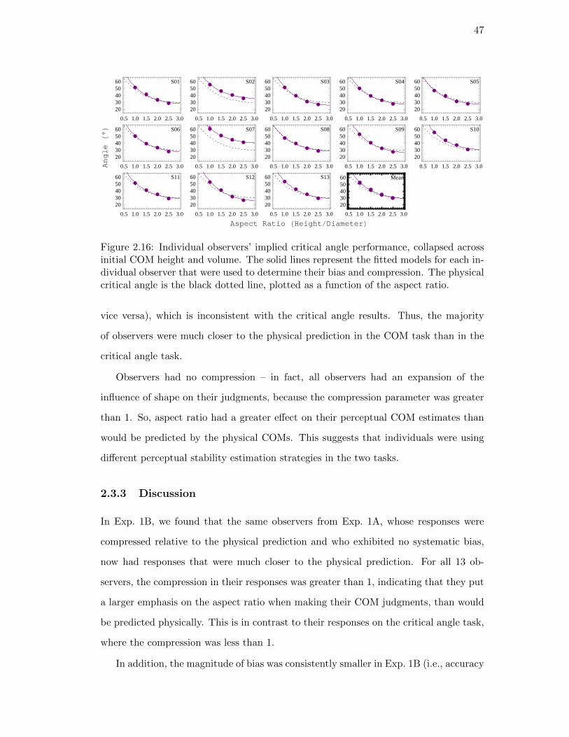
47

An

gleH

°L

æ

æ

ææ

S01

0.5 1.0 1.5 2.0 2.5 3.0

2030405060

æ

æææ

S02

0.5 1.0 1.5 2.0 2.5 3.0

2030405060

æ

æ

ææ

S03

0.5 1.0 1.5 2.0 2.5 3.0

2030405060

æ

æææ

S04

0.5 1.0 1.5 2.0 2.5 3.0

2030405060

æ

æ

ææ

S05

0.5 1.0 1.5 2.0 2.5 3.0

2030405060

æ

æææ

S06

0.5 1.0 1.5 2.0 2.5 3.0

2030405060 æ

æææ

S07

0.5 1.0 1.5 2.0 2.5 3.0

2030405060

æ

æ

ææ

S08

0.5 1.0 1.5 2.0 2.5 3.0

2030405060

æ

æ

ææ

S09

0.5 1.0 1.5 2.0 2.5 3.0

2030405060

æ

æ

ææ

S10

0.5 1.0 1.5 2.0 2.5 3.0

2030405060

æ

æææ

S11

0.5 1.0 1.5 2.0 2.5 3.0

2030405060

æ

æ

ææ

S12

0.5 1.0 1.5 2.0 2.5 3.0

2030405060

æ

æ

ææ

S13

0.5 1.0 1.5 2.0 2.5 3.0

2030405060

æ

æ

ææ

Mean

0.5 1.0 1.5 2.0 2.5 3.0

2030405060

Aspect Ratio HHeight �Diameter L

Figure 2.16: Individual observers’ implied critical angle performance, collapsed acrossinitial COM height and volume. The solid lines represent the fitted models for each in-dividual observer that were used to determine their bias and compression. The physicalcritical angle is the black dotted line, plotted as a function of the aspect ratio.

vice versa), which is inconsistent with the critical angle results. Thus, the majority

of observers were much closer to the physical prediction in the COM task than in the

critical angle task.

Observers had no compression – in fact, all observers had an expansion of the

influence of shape on their judgments, because the compression parameter was greater

than 1. So, aspect ratio had a greater effect on their perceptual COM estimates than

would be predicted by the physical COMs. This suggests that individuals were using

different perceptual stability estimation strategies in the two tasks.

2.3.3 Discussion

In Exp. 1B, we found that the same observers from Exp. 1A, whose responses were

compressed relative to the physical prediction and who exhibited no systematic bias,

now had responses that were much closer to the physical prediction. For all 13 ob-

servers, the compression in their responses was greater than 1, indicating that they put

a larger emphasis on the aspect ratio when making their COM judgments, than would

be predicted physically. This is in contrast to their responses on the critical angle task,

where the compression was less than 1.

In addition, the magnitude of bias was consistently smaller in Exp. 1B (i.e., accuracy

48

S01 S02

S03

S04

S05S06S07

S08

S09

S10

S11

S12S13

-50 0 50

0.0

0.5

1.0

1.5

2.0

Conservative�Liberal BiasH°L

Com

pres

sion

Figure 2.17: Compression and overall bias for model fits in Exp. 1A (red points) andExp. 1B (blue points). The dashed lines connect the model fits for individual observers.

is better in the COM task than stability task) and the sign of bias is not balanced across

all observers in Exp. 1B; unlike Exp. 1A, the bias tended to be more in the positive

direction. However, is the sign of the bias generally preserved across the two tasks (i.e.,

do observers with positive bias in the implied critical angles from the COM task also

tend to have positive bias in the critical angle settings)?

2.4 Experiment 2: The Role of Parts

One of the findings in Exp. 1 was that when the shape of an object is changed (such

as the manipulation of aspect ratio), observers’ stability estimates also change, but

not quite as much as would be physically predicted. (For stability judgments, the

compression parameter was consistently smaller than 1.) In Experiment 2, we consider

a different shape change, namely, the addition of a protruding part to a conical frustum.

Exp. 2 was designed to further investigate the importance of shape in this adjustment

task and to study the influence of part structure on the perceived stability of shape.

Adding parts to a shape will shift the object’s COM in the direction of the added part(s),

thereby altering the object’s stability, but how well do observers use this additional

information when judging stability?

49

2.4.1 Methods

Observers

Twelve observers at Rutgers University participated in the experiment. All were naıve

as to the purpose of the experiment, and received course credit for their participation.

Apparatus

The apparatus was the same as Exp. 1A & 1B.

Stimuli and Design

Stimuli were presented in the same rendered scene as Exp. 1A & 1B. The primary

manipulation was the addition of a part onto the object – defined using a bivariate

Gaussian distribution. The object was positioned on the table so that the part could

face towards the edge of the table or away – towards the center of the table (see

Fig. 2.18). Therefore, we had three part conditions, a baseline “no part” condition and

two conditions with the attached part: “part towards” and “part away”. The base

shapes could have one of three aspect ratios (Height/Base Diameter): 1.5, 2, and 2.5.

The conical frustum with an aspect ratio of 1 was not used because it was too short to

accommodate the attached part. The taper angle of the conical frustums was fixed at

82◦.

The method of adjustment was used to estimate observers’ perceived critical angle

for each object. Observers used the left and right arrow keys to adjust its angle of tilt

until the object was at its perceived critical angle. As in the other experiments, the

rotation of the object occurred about the point on its supporting base that was closest

to the edge of the table.

We used a 3 × 3 factorial design, with aspect ratio and part condition (“no part”,

“part towards”, and “part away”) as the independent variables. Each observer made 20

adjustments of critical angle for each combination of aspect ratio and part condition, for

a total of 180 adjustments. The initial tilt of the object, at the start of each trial, was

0◦ (vertically upright) on half the trials, and 90◦ (horizontal, rotated in the direction

50

No Part Part Towards Part Away

Figure 2.18: Cropped examples for Exp. 2 showing representative stimuli with no part(left), with the part facing towards the edge of the table (center), and with the partfacing away from the edge of the table (right).

of the precipitous edge) on the other half.

2.4.2 Results

Observer performance for the part conditions was compared to the physical predictions

for the different objects. Note that the physical predictions for the part conditions

(“part towards” and “part away” from the edge) will be different from the “no part”

condition because the presence of the part will shift the COM of the object towards the

additional mass of the part. As shown in Fig. 2.19, the “no part” condition exhibits a

similar performance trend as in Exp. 1A (underestimation of stability for lower aspect

ratios and overestimation for higher aspect ratios). In addition, we see a shift in the

perceived critical angles for conditions where a part is present, consistent with the

physical predictions – that is, higher perceived stability when the part faces away from

the edge and lower perceived stability when the part faces towards the edge8. In

addition, the higher aspect ratios exhibit a systematic overestimation, while the lower

aspect ratios exhibit underestimation (consistent with the aspect ratio-based over and

underestimation Exp. 1A).

8It should be noted that asymmetric objects, such as the frustum with part, have different criticalangles in different directions. Here we are referring here to the objects’ stability in the direction inwhich they are being tilted, namely, directly towards the precipitous edge of the table.

51

An

gleH

°L

æ

æ

ææ

ææ

æ

æ

æ

æ

æ

ææ

ææ

æ

æ

æ

1.0 1.5 2.0 2.5 3.0

10

20

30

40

50

60

Aspect Ratio HHeight �Diameter L

Figure 2.19: Group results for Exp. 2, illustrating the effects of aspect ratio, partcondition (red = “no part”, green = “part towards”, and blue = “part away”), andinitial tilt angle (solid = 0◦, dashed = 90◦). The dotted lines illustrate the physicalcritical angle curves for the respective part conditions.

As was the case in the previous experiments, there was individual variability, with

some observers having an overestimation bias and others an underestimation bias (see

Fig. 2.20). We fitted model curves to the observers’ critical angle settings – using the

model fitting technique described in Exp. 1A – for the three part conditions and overlaid

these curves on the observers’ data (see Fig. 2.21). The majority of the observers

responded in the predicted manner, taking into account the presence of the part. Next

we wished to compare the perceptual effect of the part to its physical effect on the

objects’ stability.

To evaluate the extent to which observers take into account the presence of the part

the presence of the part (regardless of any stability biases), we measured the relative

influence of the part. First, we define the influence of a part to be the difference in

critical angle between the “part away” and “part towards” conditions. We define the

relative influence to be the ratio of perceptual influence to the physical influence of a

part. If observers perfectly take into account the contribution of the part when judging

perceived stability, then the relative influence for any given aspect ratio should be 1

(i.e., the magnitude of the perceptual influence is equal to the physical influence). If

52

An

gleH

°L

æ

æ ææ

æ æ

ææ æ

æ

æ ææ æ

æ

ææ æ

S01

1.0 1.5 2.0 2.5 3.0

102030405060

æ

æ æ

æ æ æ

æ

æ ææ

æææ

æ æ

æ

ææ

S02

1.0 1.5 2.0 2.5 3.0

102030405060

æ ææ

ææ æ

æ æ ææ æ ææ æ ææ æ

æ

S03

1.0 1.5 2.0 2.5 3.0

102030405060

ææ

ææ

æ æ

ææ

ææ

æææ æ æ

æ ææ

S04

1.0 1.5 2.0 2.5 3.0

102030405060

æ

æææ æ æ

ææ

ææ

æ ææ æ

æ

ææ

æ

S05

1.0 1.5 2.0 2.5 3.0

102030405060

æ ææ

ææ æ

æ æ æææ

ææ æ æ

ææ æ

S06

1.0 1.5 2.0 2.5 3.0

102030405060

ææ

ææ æ æ

ææ æææ æ

æ æ æ

æ ææ

S07

1.0 1.5 2.0 2.5 3.0

102030405060

æ ææ

æ æ æ

ææ

æ

æ

æ æ

æ æ æ

ææ æ

S08

1.0 1.5 2.0 2.5 3.0

102030405060

æ æææ

æ æ

æ æ

æææ

ææ ææ

ææ

æ

S09

1.0 1.5 2.0 2.5 3.0

102030405060

ææ

ææ æ

æ

ææ æ

ææ

ææ æ æ

ææ

æ

S10

1.0 1.5 2.0 2.5 3.0

102030405060

ææ

ææ æ æ

ææ

æ

ææ æ

ææ æ

ææ

æ

S11

1.0 1.5 2.0 2.5 3.0

102030405060

ææ æ

ææ

æ

ææ

æ

æ

ææ

æ æ æ

ææ

æ

S12

1.0 1.5 2.0 2.5 3.0

102030405060

ææ

ææ æ æ

ææ

æ

Mean

1.0 1.5 2.0 2.5 3.0

102030405060

Aspect Ratio HHeight �Diameter L

Figure 2.20: Individual results for Exp. 2 illustrating the effects of aspect ratio, partcondition (red = “no part”, green = “part towards”, and blue = “part away”), andinitial tilt angle (solid = 0◦, dashed = 90◦). The dotted lines illustrate the physicalcritical angle curves for the respective part conditions.

there is perceptual down-weighting of the part, the relative influence should be less

than 1 (an influence of 0 would mean that the presence of the part does not affect

an observer’s stability settings at all). Alternatively, if the observer gives too much

emphasis on the part when judging the overall stability of the object, then we would

expect a relative influence greater than 1.

Fig. 2.22 shows the relative influence for each individual observer for the three aspect

ratios. Seven of the thirteen observers consistently down-weighted the influence of the

parts, three consistently over-emphasized the influence, and two wavered around the

unity line. On average, there was a slight down-weighting of the influence of the presence

of the part on perceived stability, consistent with a robust-statistics approach used to

determine the influence of a potentially separate part on global estimation (Cohen &

Singh, 2006; Denisova et al., 2006).

2.5 Conclusion

The experiments presented here suggested that people can use purely visual information

to infer the forces acting upon 3D objects in a scene. Using these inferences, observers

were able to make stability judgments using either a critical angle (Exp. 1A and 2) or

53

An

gleH

°L

æ

æ ææ æ

æ

ææ æ

1.0 1.5 2.0 2.5 3.0

102030405060

ææ æ

æ æ æ

æ

ææ

1.0 1.5 2.0 2.5 3.0

102030405060

æ ææ

ææ æ

æ æ æ

1.0 1.5 2.0 2.5 3.0

102030405060

æ

æææ

æ æ

ææ

æ

1.0 1.5 2.0 2.5 3.0

102030405060

æ

æææ ææ

ææ

æ

1.0 1.5 2.0 2.5 3.0

102030405060

ææ

ææ æ æ

ææ æ

1.0 1.5 2.0 2.5 3.0

102030405060

ææ

ææ æ æ

ææ

æ

1.0 1.5 2.0 2.5 3.0

102030405060

ææ

æ

æ æ æ

ææ æ

1.0 1.5 2.0 2.5 3.0

102030405060

ææ

ææ ææ

ææ

æ

1.0 1.5 2.0 2.5 3.0

102030405060

ææ

ææ æ æ

ææ

æ

1.0 1.5 2.0 2.5 3.0

102030405060

ææ ææ æ æ

ææ

æ

1.0 1.5 2.0 2.5 3.0

102030405060

æ

ææ

æ æ æ

ææ

æ

1.0 1.5 2.0 2.5 3.0

102030405060

ææ

ææ æ æ

ææ

æ

1.0 1.5 2.0 2.5 3.0

102030405060

Aspect Ratio HHeight �Diameter L

Figure 2.21: Individual results for Exp. 2 with data collapsed across the initial tiltangle. The red lines are the “no part” conditions, the green lines are the “part towards”conditions, and the blue line are the “part away” conditions. The dashed lines representthe model fits to the different conditions. The dotted lines illustrate the physical criticalangle curves for the respective part conditions.

COM (Exp. 1B) task.

In Exp. 1A, we showed that, on average, observers are quite accurate when making

their judgments of object stability using a critical angle task. Their visual judgments

of stability were invariant to size/volume, and appeared to be a function of only shape.

There was a bias to underestimate the stability of low aspect ratio shapes and overes-

timate the stability of high aspect ratio shapes in the average data; however, this was

due to: (i) some individual variability in bias (with some observer underestimating sta-

bility, others overestimating it) and (ii) a compression in the data curves relative to the

physical predictions (i.e., a smaller perceptual influence of aspect ratio than physically

predicted). Contrary to recent results with 2D shapes, stability judgments were not

always “on the safe side” (Samuel & Kerzel, 2011).

The critical angle results were contrasted with the COM estimates in Exp. 1B,

showing that observers were much closer to the physical prediction when they were asked

to judge the center of mass of the same objects. There was much less bias (observers

were more accurate) and the compression observed in Exp. 1A – in observers’ stability

estimates as a function of aspect ratio – was no longer present. Observers settings

of center of mass were inconsistent with their settings of critical angle and they did

54

InfluenceofPart

æ æ

æ

S01

1.0 1.5 2.0 2.5 3.0-0.5

0.00.51.01.52.0

æ ææ

S02

1.0 1.5 2.0 2.5 3.0-0.5

0.00.51.01.52.0

ææ æ

S03

1.0 1.5 2.0 2.5 3.0-0.5

0.00.51.01.52.0

ææ æ

S04

1.0 1.5 2.0 2.5 3.0-0.5

0.00.51.01.52.0

æ æ æ

S05

1.0 1.5 2.0 2.5 3.0-0.5

0.00.51.01.52.0

æ ææ

S06

1.0 1.5 2.0 2.5 3.0-0.5

0.00.51.01.52.0

æ æ æ

S07

1.0 1.5 2.0 2.5 3.0-0.5

0.00.51.01.52.0

æ æ æS08

1.0 1.5 2.0 2.5 3.0-0.5

0.00.51.01.52.0

ææ æ

S09

1.0 1.5 2.0 2.5 3.0-0.5

0.00.51.01.52.0

æ æ æ

S10

1.0 1.5 2.0 2.5 3.0-0.5

0.00.51.01.52.0

æ æ

æ

S11

1.0 1.5 2.0 2.5 3.0-0.5

0.00.51.01.52.0

ææ æ S12

1.0 1.5 2.0 2.5 3.0-0.5

0.00.51.01.52.0

æ æ æ

Mean

1.0 1.5 2.0 2.5 3.0-0.5

0.00.51.01.52.0

Aspect Ratio HHeight�DiameterL

Figure 2.22: Plots showing the relative influence of the part for individual observers.The dotted black horizontal line identifies the unity line, where observer performancewould lie if they perfectly utilized the contributions of the parts. The solid blackhorizontal line illustrates the situation where there is no influence of the presence ofthe parts on perceived stability.

not appear to rely on the COM in making judgments of physical stability. Therefore,

comparing the results, observers do not seem to be using COM – at least not in the

physically correct manner – when making judgments of object stability.

Finally, in Exp. 2, we found that observers were able to combine information from

different parts of a shape in order to judge the physical stability of objects with multiple

parts. However, even though on average observers did a very good job taking into

account the contribution of the part to the stability of the shape, there was some

down-weighting of the relative influence of the parts.

55

Chapter 3

Perception of the physical stability of asymmetrical

three-dimensional objects

3.1 Introduction

In addition to estimating the current properties of objects and surfaces based on visual

inputs, human observers are very good at predicting how objects are likely to behave

in the near future. For example, observers can visually extrapolate the trajectory of a

moving object (Becker & Fuchs, 1985; Pavel et al., 1992; Verghese & McKee, 2002), and

predict where an object that disappears behind an occluder is likely to re-emerge from

(Scholl & Pylyshyn, 1999; Graf et al., 1995; Shah et al., 2012). Even more impressive

are cases where observers can make visual predictions about object behavior based

on the inference of unseen forces, such as momentum (S.-H. Kim, Feldman, & Singh,

2012; Newman et al., 2008), gravity, and support relations (Barnett-Cowan et al., 2011;

Hamrick, Battaglia, & Tenenbaum, 2011; Samuel & Kerzel, 2011). Indeed, infants as

young as 8 months of age have been shown to be visually sensitive to support relations

and gravity; and are surprised when shown a scene in which an inadequately supported

object appears to maintain its position in space (Baillargeon & Hanko-Summers, 1990;

Baillargeon et al., 1992). Predictions such as these rely on a “causal understanding” of

the scene based on visual information (Cooper et al., 1995).

Traditional work on naıve physics has documented various ways in which people’s

intuitions are often inconsistent with Newtonian mechanics (e.g., McCloskey et al.,

1980, 1983). However, when shown dynamic “real-time” displays simulating physical

behavior, observers can be quite accurate at detecting deviations from Newtonian me-

chanics (Kaiser et al., 1985, 1992; Proffitt & Gilden, 1989). More recent work has also

demonstrated that observers correctly take into account acceleration due to gravity –

56

consistent with Newton’s laws of motion – when timing their hand movements in order

to catch a falling ball (McIntyre et al., 2001; Zago & Lacquaniti, 2005). These results

are also consistent with our day-to-day experiences of manipulating and interacting

with objects, where we are generally quite good at predicting the physical behavior

objects and guiding our motor actions.

In a recent study on the perception of object stability, Samuel and Kerzel (2011) used

planar polygonal objects, shown sitting on a supporting edge/base, with varying degrees

of “imbalance” – measured in terms of where the COM of the object lies relative to the

center of the supporting edge (including the possibility of being outside this supporting

base – in which case the object would not physically stay upright). Subjects indicated

whether a given object (shown resting on its supporting edge) would stay upright or

fall over. Their responses exhibited a conservative (or anticipatory) bias – i.e., in

the direction of perceiving an object to be unstable, even though physically it would

maintain its upright posture. These results were interpreted in terms of a conservative

tendency to keep judgments of object stability stay “on the safe side.”

In the current paper, our interest is in the visual estimation of the degree of physical

stability of 3D objects which are in stable equilibrium (in the sense that, if left unper-

turbed, they would maintain their current position). For example, the two objects in

Fig. 3.1 are both in stable equilibrium (in each case, the COM of each object is directly

above the center of a circular base). However, it is visual apparent that the object in

Fig. 3.1a is physically more stable than the one in Fig. 3.1b. In other words, based on

vision alone, one would naturally expect that the object in Fig. 3.1a is more resistant

to the action of perturbing forces than is the object in Fig. 3.1b. One natural way of

capturing object stability, therefore, is in terms of the extent to which an object can be

tilted away from its “upright” position of stable equilibrium, and maintain an unstable

equilibrium at that position where it was released. We refer to this angle of tilt as

the critical angle (see Fig. 3.2). At this angle of tilt, the center of mass (COM) of the

object is directly vertically above the point of contact on the base, around which the

object is being rotated (see Fig. 3.2b). By definition, any tilt greater in magnitude than

this critical angle will result in the object toppling over, rather than returning to its

57

ba

Figure 3.1: Two objects sitting near the edge of a table, one that is very perceptuallystable (a) and one that is very perceptually unstable (b).

upright position. With this definition in mind, it is easy to appreciate that the object

in Fig. 3.1a is physically more stable because it has a larger critical angle than the one

in Fig. 3.1b.

In previous work, we have used the visual estimation of critical angle to measure the

perception of stability for three-dimensional objects that were rotationally symmetric

(Barnett-Cowan et al., 2011; Cholewiak, Singh, Fleming, & Pastakia, 2010). While

critical angle provides a natural measure of overall physical stability for such objects,

the situation is more complicated for asymmetric 3D objects. Specifically, for an asym-

metric object, the critical angle is not a single value, but depends on the direction

in which the object is tilted. Since the object can be tilted in any radial direction

varying from 0◦ to 360◦, the critical angle is really a function defined on [0◦, 360◦).

However, as we will see, observers can reliably judge the overall stability of such an

asymmetric 3D object. This raises the question of how people combine the information

about different critical angles in different possible tilt directions into a single overall

estimate of the physical stability of an object? To address this question, we use two

experimental methods: visual estimation of critical angle in different directions (Ex-

periment 1) and perceptual matching of overall stability across objects with different

shapes (Experiment 2 & Experiment 3).

58

a

CriticalAngle

cb

Figure 3.2: Coffee cup with COMs – represented by the blue circle and blue line repre-senting gravity vector – vertically above the base (green) (a), directly over the contactpoint when the object is at its critical angle (b), and outside the base (c).

In Experiment 1, we explicitly test how well people can estimate the critical angle of

an object as a function of the direction in which the object is tilted. In Experiments 2

and 3, we ask how these different critical angles in different tilt directions are combined

into a single estimate of stability. Specifically, we compare two natural combination

rules: (i) that the overall perceived stability is determined by the average critical angle

across all possible tilt directions; (ii) overall perceived stability is determined by the

minimum critical angle (i.e., the critical angle in the least stable direction).

3.2 Experiment 1: Measuring Critical Angle in Different Directions

In the first experiment, we investigated whether observers could accurately track the

critical angle of asymmetric 3D objects as a function of the direction in which they

are tilted. The objects used in these experiments were skewed conical frustums (see

Fig. 3.3). In what follows, it will be important to distinguish between: (i) the direction

in which the object is tilted (the magnitude of tilt is adjusted interactively by the

observer); and (ii) the intrinsic direction of skew of the conical frustum objects. The

angle of relevance to us is the direction in which the object was tilted relative to

the intrinsic direction of skew of the object. We refer to this angle as α. In the

experiments, the object was always tilted directly over the precipitous edge of a table,

59

2:2 3:2 4:2

Figure 3.3: Cropped examples for Exp. 1 showing the three aspect ratios of the asym-metric conical frustums (2:2, 3:2, 4:2) with a constant skew. Note that 3D volumeswere equated and all of the objects were skewed by 25◦ from the vertical.

but the direction of intrinsic skew of the object was varied from trial to trial, thereby

manipulating α (see Fig. 3.4).

3.2.1 Methods

Observers

Fourteen Rutgers University undergraduate students participated for course credit. All

reported normal or corrected-to-normal vision.

Apparatus

The stimuli were generated in MATLAB 2012a using Psychotoolbox-3 (Brainard, 1997;

Pelli, 1997; Kleiner et al., 2007) and presented on a Sony Trinitron 20 inch CRT with

a 1024 x 768 pixel resolution at a refresh rate of 140Hz. Within Psychtoolbox-3, ex-

perimental scenes were rendered using the Matlab OpenGL (MOGL) toolbox and were

presented stereoscopically using an NVIDIA Quadro 4000 graphics card and 3D Vision

2 LCD shutter glasses. Observers were comfortably seated with a chin-rest supporting

their head 80 cm from the screen.

The individual object meshes and all relevant quantities (volumes, COM locations,

critical angles, etc.) were calculated using Mathematica 8.

60

0° 60° 120°

240° 300°180°

Figure 3.4: Examples for Exp. 1 of the 6 possible skew stimuli (α =0◦, 60◦, 120◦, 180◦, 240◦, 300◦) for a frustum with a constant aspect ratio (4:2). Notethat the aspect ratio or skew angle may appear to change in these illustrative figures;however the stimuli were presented stereoscopically, so a skew direction of α = 120◦

was facing into the screen/scene and α = 300◦ was facing out toward the observer

Stimuli and Design

The experiment used the method of adjustment to measure the perceived critical angle

for objects in a 3 aspect ratios × 6 skew directions factorial design. The objects were

conical frustums that were placed close to the edge of a virtual table. The objects had 3

possible aspect ratios (Height:Base diameter; 2:2, 3:2, 4:2) and subtended approximately

6.4-10.7 DVA (see Fig. 3.3). The frustums were skewed by 25◦ from the vertical in one

of 6 directions relative to the edge of the table (α = 0◦, 60◦, 120◦, 180◦, 240◦, 300◦) (see

Fig. 3.4). At 0◦ the object’s skew was directed towards the precipice, in the range

0◦ − 180◦ the object was facing away from the observer, at 180◦ the object was skewed

in the opposite direction of the precipice, and in the range 180◦ − 360◦ the object was

skewed toward the observer.

Objects were always tilted directly toward the edge of the table, so the skew direction

determines the tilt direction relative to the object’s intrinsic skew. The observers’

viewpoint in the scened was fixed. The objects had a woodgrain texture to reinforce

the percept of solid, uniform density objects. They were described to observers as solid

61

blocks of wood (as if cut out from the trunk of a tree). Visual cues – including shading,

a metallic reflection of the objects on the table, and dynamic lighting – were added to

aid in the realism of the scene and, in addition, scenes were presented stereoscopically.

The volumes of objects were equated across shape manipulations.

Procedure

The observers’ task was to adjust the tilt of the object until it was perceived to be

equally likely to fall off the table versus return to its upright position on the table (the

perceived critical angle). As noted previously, the object’s motion was constrained to

move orthogonal to the edge of the table, with the axis of rotation at the point on the

base of the object closest to the table’s edge.

On each trial, the conical frustum was shown with an initial tilt angle of either 0◦

(upright with base fully on the table) or 90◦ (tilted so that the entire object was over

the precipice). The starting angle was counterbalanced to later analyze for possible

hysteresis.

Each observer performed a total of 144 adjustments: 8 adjustments for each of the

3 × 6 combinations of aspect ratio and skew directions. Half of these had an initial tilt

angle of 0◦, and the other half had an initial tilt angle of 90◦.

3.2.2 Results

Observer performance was evaluated by examining their critical angle settings as a

function of the skew direction (α) and aspect ratio. A repeated measures ANOVA was

conducted on the pooled observer data, showing a highly significant effects for aspect

ratio (F (2, 26) = 86.57, p < 0.01), α (F (5, 65) = 280.31, p < 0.01), and initial tilt angle

(F (1, 13) = 11.95, p < 0.01). There was a small but significant effect of initial tilt angle

on the observers’ responses.

Fig. 3.5 shows the average data plotted as a function of α along with the predicted

critical angles for all three aspect ratios. The only notable exception was for α = 0◦

(especially at aspect ratios of 3:2 and 4:2), where observers overestimated the critical

angle (and hence the stability) of the object – which would have caused the object to

62

0 60 120 180 240 3000

15

30

45

60

75

Skew Direction HΑL

Cri

tical

Ang

leHΘ

CAL

Figure 3.5: Average group critical angle performance for the 3 object aspect ratios (red= 2:2, green = 3:2, blue = 4:2) and 6 skew directions (α = 0◦, 60◦, 120◦, 180◦, 240◦, 300◦).Dotted lines show the veridical critical angle curves for the 3 aspect ratios. Error barsare standard error. On average, observers tracked the physical critical angle quite well.

fall off the table in the real world. Observers’ settings showed that they tracked the

critical angle as a function of the skew remarkably well. Fig. 3.6 shows the individual

observers’ data plotted as a function of α.

3.2.3 Discussion

In the first experiment, we found that not only were observers able to perform the task,

they were also very good at tracking the critical angle as a function of the skew direction.

For all three aspect ratios, observers adjustments followed the physical prediction as a

function of α.

Interestingly, on average, observers’ perceptual judgments were very close to the

physical predictions, indicating that there was no systematic conservative bias for judg-

ments “on the safe side” (Samuel & Kerzel, 2011). And for α = 0◦, observers actually

made liberal critical angle estimates, suggesting that there may be a more complex in-

teraction between shape and the observers’ biases to over or underestimate the critical

63

CriticalAngleHΘCAL

S01

0 180 3000

30

60 S02

0 180 3000

30

60 S03

0 180 3000

30

60 S04

0 180 3000

30

60 S05

0 180 3000

30

60

S06

0 180 3000

30

60 S07

0 180 3000

30

60 S08

0 180 3000

30

60 S09

0 180 3000

30

60 S10

0 180 3000

30

60

S11

0 180 3000

30

60 S12

0 180 3000

30

60 S13

0 180 3000

30

60 S14

0 180 3000

30

60 Mean

0 180 3000

30

60

Skew Direction HΑL

Figure 3.6: Individuals’ critical angle response data for the 3 object aspect ratios (red =2:2, green = 3:2, blue = 4:2) and 6 skew directions (α = 0◦, 60◦, 120◦, 180◦, 240◦, 300◦).Dotted lines show the veridical critical angle curves for the 3 aspect ratios.

angle.

3.3 Experiment 2: Matching Overall Stability

3.3.1 Motivation

The results of the first experiment showed that observers tracked the critical angle as

a function of the tilt direction relative to the intrinsic skew of the object (α). However,

in addition to judging the critical angle in any given direction, observers can also

estimate overall object stability. For example, in Fig. 3.7a it is visually apparent that

the cylindrical object on the right is more stable than the skewed frustum; whereas in

Fig. 3.7b the cylindrical object is less stable.

This raises the question of how observers combine information about the various

critical angles into a unitary percept of object stability. Because the critical angle task

inherently measures the perceived stability in a single direction of tilt, we can only

answer this question by using a different task that assesses the overall stability of an

object, not just stability in a given direction. To do this, we use an overall stability

matching task.

Observers were asked to compare the overall stabilities of two objects – a standard

64

a b

Figure 3.7: Example scenes illustrating situations where a cylinder is perceptually morestable than a skewed conical frustum (a) and where a cylinder is perceptually less stablethan the skewed frustum (b).

object (corresponding to one of the skewed conical frustums from the previous experi-

ment) and a simple cylindrical comparison object – and to adjust the aspect ratio of the

comparison object until it was perceived to be equally stable as the standard. When

the stabilities of the two objects were perceptually matched, the two shapes could be

considered stability metamers.

It was not obvious a priori whether observers would be able to perform such

matches. A pilot study revealed, however, that observers find this a natural task, and

their settings are quite precise. This is consistent with the idea that physical stability

is natural perceptual dimension.

How do observers combine the various critical angles into a single stability judgment?

Two natural combination rules that could be used are: (1) to take the average of all

the critical angles; and (2) to simply use the minimal critical angle. If observers assume

that an object could have a force impulse applied from any direction (uniformly sampled

from every direction around the perimeter of the object), then it would make sense to

integrate across all possible tilt directions, which would result in the average critical

angle strategy (Hamrick et al., 2011). This average critical angle model incorporates

information from every potential force vector direction, so it can be used to take into

65

account the minimum and maximum critical angle, as well as every critical angle in-

between, when judging the overall stability.

Alternatively, observers could use the object’s minimum critical angle as a proxy for

the perceived overall stability, which may be a more salient feature if individuals are

looking for the critical angle that is most informative about a potential change in the

object’s state of equilibrium. A natural way to think of physical stability is in terms

of the minimum force required to change the equilibrium state of the object, so if we

consider the minimum of the forces in all directions, then the absolute minimum would

be in the least stable direction. That is, when a force is applied in the direction of the

minimum critical angle, it has the highest likelihood of changing the equilibrium state.

The average and minimum critical angle models were compared to see which model

better described the observers’ settings.

3.3.2 Methods

Observers

Thirteen Rutgers University undergraduate students, with normal or corrected-to-

normal visual acuity, participated in the experiment.

Stimuli and Design

The scene was composed of two objects, a standard and a comparison object, sitting

next to each other on a virtual table. The standard objects – skewed conical frustums

as in the first experiment – had 3 possible aspect ratios (2:2, 3:2, 4:2) and subtended

approximately 4.3-6.8 DVA (see Fig. 3.8). The frustums were skewed by 25◦ from

the vertical and were skewed towards the left or right (see left panes in Fig. 3.9).

In addition, the standard objects were placed on either the left or the right of the

comparison object (see center panes in Fig. 3.9). The comparison objects – cylinders –

had one of 2 initial aspect ratios (1:2 or 16:2), the two opposite ends of the aspect ratio

spectrum: short-and-wide and narrow-and-tall, that subtended approximately 3.0 and

12.3 DVA, respectively (see right panes in Fig. 3.9). They had the same wood grain

66

2:2 3:2 4:2

Figure 3.8: Cropped examples for Exp. 2 of the 3 possible aspect ratios (2:2, 3:2, 4:2)for a constant skew direction (α = 180◦), with the comparison cylinder at it’s lowestaspect ratio (1:2) on the right.

texture and material properties as the conical frustums and had a variable aspect ratio,

to be adjusted by the observers.

The experiment used the method of adjustment for stability matching using a 3

standard aspect ratios × 2 skew directions × 2 presentation locations × 2 initial com-

parison object aspect ratios factorial design.

Procedure

On each trial, a standard conical frustum was shown alongside a comparison cylinder.

The observers’ task was to adjust the aspect ratio of the comparison object until it

was judged to have the same overall stability as the standard object. The comparison

object’s volume was held constant across changes in aspect ratio, hence the observer’s

adjustments affected both height and radius. Since the two objects had the same surface

properties and there were no other stability cues than the visual ones, observers had to

rely on shape alone in making their judgments.

When the observer finished their aspect ratio adjustment (i.e., when the perceived

stabilities of the comparison and standard were subjectively the same), the two objects

could be considered stability metamers (similar to color metamers, where two colors are

67

Initial Comparison

Aspect Ratio = 16:2

Initial Comparison

Aspect Ratio = 1:2

Standard α = 0°

Standard α = 180°

Standard on

Left

Standard on

Right

Figure 3.9: Examples of the two standard skew directions (α = 0◦and180◦), the twostandard object locations (left and right), and the 2 initial comparison aspect ratios(1:2 and 16:2).

perceived to be the same even though they have differing wavelength compositions).

Each observer performed a total of 192 adjustments: 8 adjustments for each of the

3 × 2 × 2 × 2 combinations of aspect ratio, skew direction, presentation location, and

initial comparison aspect ratio.

3.3.3 Results

A repeated measures ANOVA was conducted on the pooled observer data, showing

significant effects for the standard aspect ratio (F (2, 24) = 50.80, p < 0.01) and initial

comparison aspect ratio (F (1, 12) = 21.12, p < 0.01) (see Fig. 3.10). There was no

effect of skew direction (F (1, 12) = 3.67, p > 0.05) or presentation location (F (1, 12) =

1.23, p > 0.05). There was a small but significant effect of initial aspect ratio on the

observers’ responses (see Fig. 3.11 for individual observers’ data). Further analyses

were collapsed across initial comparison aspect ratio.

Observers’ settings were compared against predictions derived from (i) the average

critical angle model and (ii) the minimum critical angle model. If observers used the

lowest critical angle to make their judgments, then we would expect their data to

be close to the minimum critical angle prediction (blue dashed curves in Fig. 3.10 &

68

0.5 1 1.5 2 2.50

2

4

6

8

Standard Aspect Ratio

Com

pari

son

Asp

ectR

atio

Figure 3.10: Average group performance for the 3 object aspect ratios (2:2, 3:2, 4:2)collapsed across skew direction and presentation location. The green lines represent theobservers’ responses, separated by initial comparison aspect ratio (solid = 16:2, dashed= 1:2). The blue line represents the predicted comparison aspect ratio if observers usedthe minimum critical angle and the red line represents the average prediction. Errorbars represent 95% confidence intervals.

Fig. 3.11). Conversely, if observers used an estimate that uniformly took into account

the object’s critical angle in all possible directions, then their judgments should be closer

to the average critical angle prediction (red dashed curves in Fig. 3.10 & Fig. 3.11).

On average, the observers’ settings were closer to the minimum critical angle model’s

predictions than the average critical angle model.

In order to evaluate which model (average critical angle or minimum critical angle)

better described observers’ performance, we calculated the likelihood ratios for each ob-

server’s data. The likelihood ratio test allows us to compare the two stability estimation

models and judge which model better explains the observed data.

Normally, we would compare performance using the Bayes factor (K), which is

the ratio of the probability of the data given the first model (Pr(D|Mavg)) over the

probability of the data given the second model (Pr(D|Mmin))(see Eq. 3.1).

69

ComparisonAspectRatio

S01

0.5 1 1.5 2 2.502468

S02

0.5 1 1.5 2 2.502468

S03

0.5 1 1.5 2 2.502468

S04

0.5 1 1.5 2 2.502468

S05

0.5 1 1.5 2 2.502468

S06

0.5 1 1.5 2 2.502468

S07

0.5 1 1.5 2 2.502468

S08

0.5 1 1.5 2 2.502468

S09

0.5 1 1.5 2 2.502468

S10

0.5 1 1.5 2 2.502468

S11

0.5 1 1.5 2 2.502468

S12

0.5 1 1.5 2 2.502468

S13

0.5 1 1.5 2 2.502468

Mean

0.5 1 1.5 2 2.502468

Standard Aspect Ratio

Figure 3.11: Individual observer performance for the 3 object aspect ratios (2:2, 3:2, 4:2)collapsed across skew direction and presentation location. The green lines represent theobservers’ responses, separated by initial comparison aspect ratio (solid = 16:2, dashed= 1:2). The blue line represents the predicted comparison aspect ratio if observers usedthe minimum critical angle and the red line represents the average prediction. Errorbars represent 95% confidence intervals.

K =Pr(D|Mavg)

Pr(D|Mmin)(3.1)

However, in this case the two models we are comparing have no free parameters,

which means the Bayes Factors simply reduces to the ratio of the two model likelihoods.

This likelihood ratio can now be used to judge which model better explains the data,

with likelihood ratio values greater than 1 supporting Mavg and values less than 1

supporting Mmin. The ratios of the average and minimum likelihoods were calculated

for each observer (see Eq. 3.2). Because the raw likelihoods can be extremely small or

large, we calculated the log likelihoods for the individual models and for the likelihood

ratios – meaning positive log likelihoods support Mavg and negative log likelihoods

support Mmin.

Λobserver =

∏ni=1 Pr(Di|Mavg)∏ni=1 Pr(Di|Mmin)

(3.2)

For 10 of the 13 observers, the calculated log likelihood ratios supported the mini-

mum model over the average model (see Table 3.1), indicating that the minimum crit-

ical angle provides a better model of the observers’ stability matches than the average

70

Table 3.1: Log likelihoods for each model and the log likelihood ratios(Log(Likelihoodavg/Likelihoodmin)) for each observer. Note that for 10 of the 13observers, the log likelihood ratio favored the minimum model – that is, the likelihoodratio was negative.

Observer Log(Likelihoodavg) Log(Likelihoodmin) Log(Λ) Model Favored

1 −507.33 −154.81 −352.51 Minimum2 −1920.61 −374.93 −1545.69 Minimum3 −561.97 −218.72 −343.25 Minimum4 −1094.45 −258.80 −835.66 Minimum5 −328.60 −213.95 −114.65 Minimum6 −1659.79 −254.89 −1404.89 Minimum7 −367.33 −243.18 −124.15 Minimum8 −585.69 −246.68 −339.01 Minimum9 −1054.09 −116.44 −937.65 Minimum10 −683.06 −218.44 −464.62 Minimum11 −8317.27 −29086.70 20769.40 Average12 −270.65 −3203.57 2932.92 Average13 −231.59 −702.86 471.27 Average

critical angle.

3.3.4 Discussion

Observers’ judgments were better explained by the minimum critical angle, rather than

the mean critical angle. Thus the least-stable direction has a disproportionately large

influence in visually estimating the overall stability of an object. The direction of

least stability could be considered the “worst case scenario” and it tends to dominate

observers’ judgments.

3.4 Experiment 3: Matching Overall Stability in Different Directions

3.4.1 Motivation

The results of the stability matching task in Experiment 2 indicated that observers’

overall stability judgments were informed by the minimum critical angle of the asym-

metric objects. The idea behind the stability matching task presented in Exp. 2 was

that, unlike the critical angle task, the stability matches for a given object should be

stable as the direction of tilt varies relative to the intrinsic skew of the object. Here we

71

test if this is indeed the case.

Dependencies on the viewing direction are common in 3D shape perception – and

are particularly acute when the axis of elongation of an object is foreshortened (Marr &

Nishihara, 1978; Biederman, 1987; Humphrey & Jolicoeur, 1993; Lawson & Humphreys,

1998). Because of this, one may expect some effect of viewing direction on visual

judgments of object stability (if the shape appears different, its perceived stability will

of course also be affected). However, we would expect that any such effects are much

smaller than the large influence of skew direction on perceived critical angles, observed

in Experiment 1.

In this experiment, observers compared the overall stabilities of two objects – a

standard and a comparison – and adjusted the comparison object until it was perceived

to be the same stability as the standard, just as in Exp. 2. However, this experiment

differed from Exp. 2 in that the direction of skew was also manipulated (analogous to

the manipulation of α in the first experiment).

3.4.2 Methods

Observers

Thirteen Rutgers University undergraduate students, with normal or corrected-to-

normal visual acuity, participated in the experiment.

Stimuli and Design

The experiment used the same stability matching task as Exp. 2. It used a 3 standard

aspect ratios × 6 skew directions × 2 presentation locations × 2 initial comparison

object aspect ratios factorial design.

As in the second experiment, the rendered scene contained two objects, a standard

and a comparison object, sitting next to each other on top of a table. The standard

objects had 3 possible aspect ratios (2:2, 3:2, 4:2), were skewed by 25◦ from the vertical,

and were skewed in 1 of 6 skew directions (0◦, 60◦, 120◦, 180◦, 240◦, 300◦). In addition,

the standard objects were placed on either the left or the right of the comparison object

72

and the comparison objects had one of two initial aspect ratios (1:2 or 16:2). See Fig. 3.9

for examples of the scene layout.

Procedure

The testing procedure was identical to Experiment 2.

Each observer performed a total of 216 adjustments: 6 adjustments for each of the

3 × 6 × 2 combinations of aspect ratio, skew direction, and presentation location. Half

of these used an initial aspect ratio of 1:2 for the comparison object; the other half used

an initial aspect ratio of 16:2.

3.4.3 Results

Observer performance was evaluated by examining their stability matches (aspect-ratio

settings for the comparison object) as a function of the skew direction. A repeated

measures ANOVA was conducted on the pooled data, showing a highly significant

effect of aspect ratio (F (2, 24) = 153.21, p < 0.01) and a significant effect of initial

comparison aspect ratio (F (1, 12) = 7.53, p < 0.05). There was also a significant effect

of skew direction (F (5, 60) = 39.94, p < 0.01), but a Post-Hoc Tukey Test confirmed

that the slant direction effect was due to the dip in performance at 60◦ and 120◦ and

that there were no other significant differences for any other slant directions.

As shown in Fig. 3.12, on average, judgments were affected by the change in the

standard aspect ratio and the direction of the skew, which had a much smaller effect.

There was a slight dip in the comparison aspect ratios at 60◦ and 120◦. It is likely this

may have been due to perceived foreshortening when the slant was directed into the

screen.

3.4.4 Discussion

The results from the third experiment support the hypothesis that observers are able

to match the overall stabilities of objects in a consistent manner, even when the asym-

metric objects are rotated relative to the observer’s viewpoint.

73

0 60 120 180 240 3000

2

4

6

8

Skew Direction Α HDegreesL

Com

pari

son

Asp

ectR

atio

Figure 3.12: Average group performance in Exp. 3 for the 3 object aspect ratios (red =2:2, green = 3:2, blue = 4:2) collapsed across the other independent variables (standardlocation and initial comparison aspect ratio) as a function of the skew direction. Thedashed lines represent the minimum critical angle predictions for each aspect ratio.Error bars represent standard error.

Although the effect of skew direction was statistically reliable, it was quite small

when compared to the influence of skew direction on the perceived critical angle ob-

served in Exp. 1. Given the well-known effects of foreshortening of the axis on shape

perception, it seems likely that the observed influence of skew direction on perceived

stability is most likely due to the misperception of 3D shape from those viewpoints

(Marr & Nishihara, 1978; Biederman, 1987; Humphrey & Jolicoeur, 1993; Lawson &

Humphreys, 1998). Nevertheless, the stability matches are surprisingly flat, especially

when compared with the large influence of skew direction on the perceived critical angles

observed in Exp. 1.

74

3.5 Conclusion

The critical angle is a good measure of stability for three-dimensional objects, incor-

porating information about mass distribution and shape to define an ecologically im-

portant property of real-world objects. We have previously found that people are good

at visually estimating the critical angles of symmetric objects (Barnett-Cowan et al.,

2011; Cholewiak et al., 2010); however, it was not clear how these results would extend

to more general, asymmetric objects. Since the critical angle is not a single value for

asymmetric objects, but depends on the direction in which the object is tilted, we in-

vestigated how well observers could visually estimate the critical angles in different tilt

directions for asymmetric objects.

Observers were clearly able to track the critical angle as asymmetric conical frustums

were tilted in different directions relative to their intrinsic skews in Exp. 1, indicating

that their judgments were appropriately informed by the shape’s asymmetry. These

results extend our previous results for rotationally symmetric objects to asymmetric

objects. This is reassuring because anecdotally we have few issues making guided

actions that are informed by our percepts of real-world object stability. In contrast

to the findings of Samuel and Kerzel (2011) with 2D polygonal objects, however, our

results show no systematic conservative bias – i.e., for stability settings to be judged

“on the safe side”.

Although our Exp. 1 results showed that individuals could reliably judge stability,

as reflected in the work by Samuel and Kerzel (2011), there was an important con-

trast: observers did not always make their critical angle judgments “on the safe side”.

In fact, although Samuel and Kerzel (2011) found that their observers systematically

made conservative judgments – judging the objects to be less than physically stable,

observers in our experiments were quite accurate at visually estimating physical sta-

bility. Although there was of course some individual variability across observers (with

some tending to overestimate and others tending to underestimate stability), we did

not see any systematic conservative bias in the pooled data.

Surprisingly, observers were able to reliably match the perceived stability of two

75

objects with different shapes in Exp. 2. These results suggest that stability may be

represented along a unitary dimension. The observers were able to infer the force of

gravity acting upon the shapes and compare their overall stabilities even though the

shapes were quite different. Observers’ stability matches were better explained by the

minimum model than the average model, suggesting that observers’ estimates were

disproportionately influenced by the direction of least stability. Since physical stability

is defined as the minimum force required to change the equilibrium state of the object,

the direction with the smallest critical angle defines where the object has the highest

likelihood of changing its equilibrium state. Although the average critical angle is a

measure of the central tendency of the stability for the object – taking into account the

maximum and minimum stability, and all of the critical angles in-between – on average,

people appeared to use the minimum critical angle as a proxy for the perceived overall

stability.

Finally, Exp. 3 demonstrated that the matches were a function of the aspect ratio of

the 3D shapes – with observed data exhibiting only a slight dependence on viewpoint

(likely due to foreshortening).

As a whole, these results are evidence that visual estimates of overall object stability

are strongly influenced by the minimum critical angle and that perceived shape plays

an important role to inform the people of the objects’ physical properties.

76

Chapter 4

Visual adaptation to the physical stability of objects

4.1 Introduction

How does the brain represent Newtonian forces? It has been suggested by research in

naıve – intuitive – physics that people incorrectly infer forces and object motion due

to faulty internal models (McCloskey et al., 1980; McCloskey, 1983b, 1983a). However,

there is an alternative body of research that has shown that while people make mistakes

when relying upon higher-level, slower reasoning, their lower level perceptual judgments

are much more consistent with physically accurate models – especially when they are

shown real-time simulations of physical behavior (Kaiser et al., 1985, 1992; Proffitt &

Gilden, 1989). We have previously demonstrated that judgments of object stability are

fairly consistent with physical predictions (Cholewiak et al., 2010; Cholewiak, Fleming,

& Singh, 2011, 2012); here we show clear evidence in support of lower level representa-

tion of perceived stability, demonstrating that stability – and the inference of forces –

is likely an perceptual attribute that is subject to adaptation effects.

People can usually judge, based on vision alone, whether an object is physically

stable or unstable; that is, whether it will stay in its current physical state or fall

due to gravity. Anecdotally, these stability judgments appear to occur automatically

and unconsciously, and we seem quickly identify these salient situations where objects

appear unstable (for example, see Fig. 4.1).

The perception of physical stability requires the inference of forces in order to judge

whether or not an object will fall. Previous work has documented observers’ ability

to estimate object stability (Barnett-Cowan et al., 2011; Cholewiak et al., 2010, 2011,

2012; Samuel & Kerzel, 2011) and has shown that people use aspects of shape – such

as aspect ratio and part structure –when making stability judgments. Cholewiak et

77

(a) Stones balanced at Aghna-cliff dolmen in Ireland (Dempsey,2008)

(b) Bricks carefully balanced(Dan, 2007)

(c) Former Transport Ministryof Georgia (Zollinger, 2008)

Figure 4.1: Photographs illustrating how scenes can convey the physical interactionsand support relations between objects in a scene. Sometimes the support structuresand interactions are clear, (a) and (b). Other times, foundations conceal the forces thatsupport the objects, (c).

al. (2012)’s results suggest that perceived stability may be represented as a unitary

dimension, where objects are perceptually judged on a continuum from very unstable to

stable. The ability to make judgments of a object’s critical angle or its COM, however,

does not necessarily imply that object stability is a natural perceptual dimension. So, in

the experiments described herein, we asked whether it is possible to obtain adaptation

aftereffects with perceived object stability.

Color, motion, and prismatic aftereffects have long been used as evidence for the

claim that visual perception operates at an earlier stage of processing (Harris, 1963;

Singer & Day, 1966a, 1966b) and that there are specific neuronal pools dedicated to

the representation of perceptual variables. The reliability of perceptual adaptation –

continued exposure to previously explored stimuli affecting the neural representation

– has led to aftereffects to being dubbed the psychophysicists microelectrode. Recent

neuroscience studies have supported these claims and have shown that perceptual af-

tereffects lead to neuronal response rate tuning in both non-humans (Dragoi, Sharma,

& Sur, 2000; Dragoi, Sharma, Miller, & Sur, 2002; Kohn & Movshon, 2003, 2004) and

humans (Tootell et al., 1995). Recently, there has also been research demonstrating

that some processes that were traditionally held to be dependent upon higher-level

processing, specifically visual judgments of numerosity, may be represented at a lower

perceptual level than traditionally believed (Burr & Ross, 2008; Burr, Anobile, & Turi,

2011).

78

We want to answer the question of whether judgments of stability are purely based

on high-level knowledge/reasoning, or may they be represented perceptually? In the

following experiments, we test whether perceived stability is indeed a bona fide unitary

perceptual dimension that is susceptible to adaptation aftereffects.

4.2 Experiment 1: 2D Curvature Probe

In the first experiment, we tested whether visually adapting to stable and unstable

shapes would lead to a stability aftereffect that causes under and overestimation, re-

spectively, of the perceived stability of test shapes. When observers adapt to stable

shapes (see Fig. 4.2), a stability aftereffect would cause them perceive test shapes as

less stable and vice versa, if they adapt to unstable shapes, they will perceive the test

shapes as more stable. The test shapes in Exp. 1 had axes with variable curvature and

constant rib-lengths (see Fig. 4.3). The curvature of the object’s axis was increased

while its base remained fully in contact with the ground plane/supporting surface.

With sufficiently high curvature, the COM would no longer lie above the object’s base;

and the object would become unstable (i.e., would no longer physically stay upright).

Thus the curvature manipulation allowed us to manipulate the stability of the shape in

a controlled manner.

4.2.1 Methods

Observers

Ten Rutgers University students. All reported normal or corrected-to-normal vision.

Apparatus

The stimuli were generated in MATLAB 2012a using Psychtoolbox-3 (Brainard, 1997;

Pelli, 1997; Kleiner et al., 2007) and presented on a Sony Trinitron 20 inch CRT with

a 1024 x 768 pixel resolution at a refresh rate of 140Hz. Observers were comfortably

seated with a chin-rest supporting their head 80 cm from the screen.

79

a

b

Figure 4.2: Examples of the 2D adaptation stimuli. The stimuli in the top row (a) areexamples of very stable shapes, while the stimuli in the bottom row (b) are examplesof very unstable shapes. Note that the shapes in row (a) were vertically flipped in theexperiment to produce very unstable adaptation shapes (not illustrated in this figure).

The individual object contours and all relevant quantities (areas, COM locations,

critical angles, etc.) were calculated using Mathematica 8.

Adaptation Stimuli

The adaptation shapes were 2D silhouettes that were either very stable – bottom heavy

with very high critical angles – or very unstable – top heavy with very low or negative

critical angles (negative meaning that the shapes would not physically stand up as

presented) (see Fig. 4.2). The silhouettes were placed on horizontal supporting surface

– a “table” composed of 3 rectangles. In order to ensure that any adaptation was due

to the perceived stability and not an artifact of the specific shapes used, the same set

of shapes was used for both the high and low stability adaptation conditions; they were

simply rotated through 180◦.

The adaptation shapes were constrained to have a fixed area. The contours of the

80

left and right sides of the shape were analytically defined using B-spline functions with 7

control points each, while the top and bottom were straight horizontal lines connecting

the endpoints of the B-splines, ensuring that the shapes could be flipped vertically.

Unique adapting shapes were generated by randomly varying the control points of the

B-spline functions. The final set of 45 adapting stimuli were picked by selecting the sets

of B-spline functions that created shapes with constant area and critical angles greater

than 50◦ (Range = [50.33◦, 73.03◦],M = 63.52◦, SD = 5.37◦).

The low stability shapes were the same 45 shapes, vertically flipped. By vertically

flipping the high stability stimuli, we were able to create a series of unstable shapes that

either had small or negative (completely unstable) critical angles. The critical angles

for the unstable stimuli ranged from −21.69◦ to 17.90◦ (M = 3.60◦, SD = 10.57◦).

Test Stimuli

We wanted a novel set of shapes that would allow us to probe the observers’ judgments

of stability. The base shape that we used for probing the observer’s judgments was an

analytically-defined, vertically symmetric elongated shape with a rounded bulge at the

top, making it top heavy (see Fig. 4.3).

We manipulated the test shape’s stability by adding different levels of curvature to

its primary axis while constraining its thickness function along the axis of symmetry

(Biederman, 1987; Blum, 1967; Feldman & Singh, 2006; Marr & Nishihara, 1978). With

no curvature, the object was vertically upright and stable (critical angle = 10.52◦ in

either direction) (see shape a in Fig. 4.3). Increasing the curvature of the primary axis

bent the shape, shifting the object’s COM. The physical stability – defined using the

critical angle – decreased as the curvature increased, as the horizontal position of the

COM approached the edge of the object’s base. Once the COM was no longer vertically

above the base, the object was unstable and would not stay upright, as presented (see

shape c in Fig. 4.3). The curvature where the object was equally likely to stay upright

or fall – when the COM was directly over the edge of the base – was defined as the

tipping point (see shape b in Fig. 4.3).

A set of 201 versions of the test shape were generated, with curvatures ranging from

81

a b c

�1.0 �0.5 0.5 1.0

0.2

0.4

0.6

0.8

1.0

�1.0 �0.5 0.5 1.0

0.2

0.4

0.6

0.8

1.0

�1.0 �0.5 0.5 1.0

0.2

0.4

0.6

0.8

1.0

Figure 4.3: Examples of the 2D curvature test shapes. The top shapes show examplesof the stimuli shown to observers and the bottom plots illustrate how the shapes’ axeswere curved while ribs were kept perpendicular to their axis tangents. The left-mostshape (a) has the minimum curvature and is completely stable, the right-most shape(c) has the maximum curvature and is completely unstable, and the center shape (b)is at its tipping point.

0 DV A−1 to 0.54 DV A−1. The critical curvature (“tipping point”) for the test shape

was 0.28 DV A−1. The curvatures were converted to a 0 to 2 scale, where 0 was no

curvature (0 DV A−1) and 2 was the maximum curvature presented (0.54 DV A−1),

making the critical curvature 1.04. During the experiment, the test shape was shown

curved either to the left or the right.

Design

The experiment used a yes/no paradigm, where observers were asked to judge whether a

test stimulus would stay upright or fall over. There were a total of four conditions, a pre-

test with no adaptation, the two adaptation conditions counterbalanced across subjects,

and a post-test without adaptation. Observers completed the baseline condition, a

single adaptation condition, took a 5 minute break, completed the second adaptation

condition, and finished with the post-test.

Observers were instructed to judge whether the test shapes would fall or stay upright

(by pressing “f” if the shape would fall and “j” if the shape would stay upright).

82

They were shown an example of an extremely stable test shape (curvature = 0) and

an extremely unstable test shape (curvature = 2) to illustrate the range of possible

curvatures. In addition, they were instructed to judge each shape as if it were a frame

from a movie, where the object could fall or stay upright in the next frame. Observers

were given 10 practice trials and all observers confirmed that they understood the task

and felt that they could readily judge whether a shape would fall or stay upright.

For each condition, stimuli were chosen using the Psi adaptive staircase method, de-

scribed by Kontsevich and Tyler (1999), implemented in MATLAB with the Palamedes

toolbox (Kingdom & Prins, 2010). The Psi method allows for estimation of the point

of subjective equality (PSE) – the tipping point in these experiments – and slope – the

difference threshold – of the psychometric function for observers’ judgments.

For the pre-test condition, observers were shown a fixation cross for 1000 ms, a test

stimulus – drawn from the pool of 201 test curvatures (selected using the Psi adaptive

staircase method) and randomly curved to the left or right – for 250 ms, and then

a screen with only the “table” and were asked to respond if the test stimulus would

fall or stay upright. A total of 50 trials were shown for the pre-test, with a forced

break between the 25th and 26th trials. After confirming that the observer had a clear

understanding of the task, he/she then began either the stable or unstable adaptation

condition (counterbalanced across subjects).

In the adaptation conditions, we used a top-up procedure to adapt observers to

either stable or unstable shapes (Hong & Papathomas, 2006; Burr et al., 2011). For the

first trial, observers were shown a fixation cross for 1000 ms, a series of 40 adaptation

stimuli – drawn randomly without replacement from the 45 generated – that were shown

for 500 ms each (20 seconds total), another fixation cross for 500 ms, a test stimulus

for 250 ms, and then a screen with only the table and were asked to respond if the test

stimulus would fall or stay upright. Subsequent to the first trial, the adaptation was

topped up by showing a sequence of 10 adapting shapes prior to each test shape. This

was repeated until the break, after which observers were shown another random series

of 45 shapes, with the 10 shape top-up procedure for the subsequent trials.

83

4.2.2 Results

The Psi method was used to estimate the observers’ PSEs for each condition with 95%

confidence intervals (Kingdom & Prins, 2010). The pre-test condition data were found

to be noisy for most observers – with large 95% confidence intervals and non-converging

data, presumably because most observers were naıve to the testing procedure and used

the pre-test as an extended “practice” –, so only the adaptation conditions were used

for further analysis. Because the post-test condition immediately followed the second

adaptation condition, it was excluded due to potential residual adaptation aftereffects.

A shift in the adaptation condition PSEs could indicate the presence of priming –

i.e., judgments biased in the direction of the adapting shapes – or of an aftereffect –

where adaptation leads to judgments in the opposite direction of the adapting shapes.

Seven out of 10 observers had significantly different PSEs for the Stable and Unsta-

ble Adaptation conditions (PSEs for each condition fell outside of the 95% confidence

intervals for the other condition). Fig. 4.4 illustrates the individual observers’ PSEs,

standardized by removing the bias. And, as predicted, all of the observers with signifi-

cant differences were biased to underestimate stability after adapting to high-stability

shapes and overestimate stability after adapting to low-stability shapes – consistent

with a stability aftereffect.

In addition, bias was measured for each observer by averaging the two adaptation

conditions to see if there was a systematic under or overestimation bias. As shown in

Fig. 4.5, 7 out of 10 of the observers underestimated the stability on average while the

other 3 overestimated stability, with an average PSE of 0.97 (0.26 DV A−1), which is

below the physical tipping point of 1.04 (0.28 DV A−1). Although there was a bias to

underestimate stability, it was not large.

4.2.3 Discussion

The observers in Exp. 1 exhibited a stability aftereffect when asked if the curved test

shape would fall or stay upright. After viewing highly stable shapes, they judged test

shapes with lower curvature to be unstable and after viewing highly unstable shapes,

84

æ

æ

æ

æ

æ

æ

æ

æ

æ

æ

æ

æ

æ

æ

æ

æ

æ

æ

æ

æ

-0.6 -0.4 -0.2 0.2 0.4 0.6Curvature

2

4

6

8

10

Subject

Blue = Stable Adaptation

Red = Unstable Adaptation

Figure 4.4: PSE results using 2D curvature test shapes standardized by removing bias(average PSE for the adaptation conditions). Subjects (y-axis) were sorted by magni-tude of the aftereffect (PSE for Unstable Adaptation - PSE for Stable Adaptation), withindividuals showing the smallest aftereffect at the bottom and those with the largestat the top. Note: Curvatures are presented using a 0 (0 DV A−1) to 2 (0.54 DV A−1)scale.

they would judge test shapes with higher curvature to be stable. This means that their

percept of the tipping point is affected by the stability of the adapting shapes and that

the shift in their percept is consistent with a stability aftereffect prediction (rather than

priming).

4.3 Experiment 2: 2D Shift Probe

Exp. 1 showed that observers shifted their perceived tipping point when they were shown

highly stable or unstable adapting stimuli. We wanted to test the robustness of our

finding by making sure that it wasn’t somehow specific to the curvature manipulation.

Therefore, in Exp. 2, we used test shapes that provided a very different manipulation of

shape (top/bottom shift) that could also be used to demonstrate a stability aftereffect

when judging the tipping point of shapes.

85

Overestimating StabilityUnderestimating Stability

æ

æ

æ

æ

æ

æ

æ

æ

æ

æ

0.5 1.0 1.5 2.0Curvature

2

4

6

8

10

Subject

Figure 4.5: Bias results for the 2D curvature experiment. Subjects (y-axis) have thesame ordering as in Fig. 4.4, where individuals showing the smallest aftereffect are atthe bottom and those with the largest at the top. Note that the vertical dashed lineis the physical tipping point for this test measure. Note: Curvatures are presentedusing a 0 (0 DV A−1) to 2 (0.54 DV A−1) scale, with the critical curvature at 1.04(0.28 DV A−1).

4.3.1 Methods

Observers

Ten Rutgers University undergraduate students. All reported normal or corrected-to-

normal vision.

Apparatus

As in Exp. 1, the stimuli were generated in MATLAB 2012a using Psychtoolbox-3 and

observers were comfortably seated with a chin-rest 80 cm from the screen.

Adaptation Stimuli

The adaptation shapes were identical to the 2D adaptation shapes used in Exp. 1,

either very stable – bottom heavy with very high critical angles – or very unstable –

top heavy with very small or negative critical angles (see Fig. 4.2 for examples). And

as in Exp. 1, a total of 45 unique high stability adapting shapes were generated, with

unstable shapes being the same objects turned upside-down.

86

a b c

�1.0 �0.5 0.5 1.0

0.2

0.4

0.6

0.8

1.0

�1.0 �0.5 0.5 1.0

0.2

0.4

0.6

0.8

1.0

�1.0 �0.5 0.5 1.0

0.2

0.4

0.6

0.8

1.0

Figure 4.6: Examples of the 2D shift test shapes. The top shapes show examples ofthe stimuli shown to observers and the bottom plots illustrate how the axes bent asthe B-spline control points were shifted. The left-most shape (a) has the no shift andis completely stable, the right-most shape (c) has the maximum shift presented and iscompletely unstable, and the center shape (b) is at its tipping point.

Test Stimuli

The primary differences from Exp. 1 were the base shape and the transformation

used for probing the observer’s judgments. For this experiment, the object was an

analytically-defined bar-bell-like shape with a rounded bulge at both the top and the

bottom (see Fig. 4.6). The top was slightly rounded while the bottom had a flat bottom.

The test shapes were manipulated by shifting the top and bottom parts in opposite

directions, so that as the lateral separation between the top and bottom increased, the

shape would become less stable. In order to give the perceptual appearance of the top

and bottom moving in opposite directions, the test shape was manipulated by shifting

the B-spline functions’ control points, rather than simply applying a skew to the object.

Each side of the shape was composed of 7 control points, with the first 6 of each side

defining the barbell shape and the 7th shared as the top-most point. To apply the shift,

the bottom 2 points for the left and right functions were moved in one direction and

the top 3 points were moved in the opposite direction, while the 3rd and 4th points were

kept stationary. This lead to the object shifting its top and bottom features without

87

introducing a strong perceived skew (see Fig. 4.6).

With no shift, the object was vertically upright and stable. Increasing the lateral

shift between the top and bottom shifted the location of the COM relative to the

supporting base. So, as the shift increased, the physical stability – defined using the

critical angle – decreased. And as with the curvature measure, once the COM was no

longer vertically above the base, the object was unstable and would not stay upright as

presented. The magnitude of lateral shift for which the object was equally likely to stay

upright or fall – when the COM was directly over the edge of the base – was defined as

the tipping point.

51 test stimuli were generated with shifts ranging from 0 DV A to 3.72 DV A. The

tipping point for these test shapes was 1.79 DV A (see shape b in Fig. 4.6). The shifts

were converted to a 0 to 0.5 scale, where 0 was no shift (0 DV A) and 0.5 was the

maximum shift presented (3.72 DV A), making the critical lateral shift 0.24. During

the experiment, the top of the test shape was shifted either to the left or the right.

Design

As in Exp. 1, this design used a yes/no paradigm to judge if the test stimulus would

stay upright or fall. There were four conditions, a pre-test with no adaptation, the

two adaptation conditions counterbalanced across subjects, and a post-test without

adaptation. As in Exp. 1, observers completed the baseline condition, a single adapta-

tion condition, took a 5 minute break, completed the second adaptation condition, and

finished with the post-test.

The experimental procedure was the same as in Exp. 1.

Stimuli were chosen using the Psi adaptive staircase method so that we could esti-

mate the PSE – the tipping point in these experiments – of the psychometric function

for observers’ judgments. In the adaptation conditions, we used the same top-up pro-

cedure to adapt observers to either high-stability or low-stability shapes as was used in

Exp. 1.

88

æ

æ

æ

æ

æ

æ

æ

æ

æ

æ

æ

æ

æ

æ

æ

æ

æ

æ

æ

æ

-0.2 -0.1 0.1 0.2Shift

2

4

6

8

10

Subject

Blue = Stable Adaptation

Red = Unstable Adaptation

Figure 4.7: PSE results using a 2D shift test shape standardized by removing bias (av-erage PSE for the adaptation conditions). Subjects (y-axis) were sorted by magnitudeof the aftereffect (PSE for Unstable Adaptation - PSE for Stable Adaptation), withindividuals showing the smallest aftereffect at the bottom and those with the largestat the top. Note: Lateral shifts are presented using a 0 (0 DV A) to 0.5 (3.72 DV A)scale.

4.3.2 Results

The Psi method was used to estimate the observers’ PSEs with 95% confidence inter-

vals (Kingdom & Prins, 2010). All 10 subjects showed an effect of adaptation in the

expected direction, i.e. all were biased in the direction of underestimating stability

after adapting to stable objects and overestimating stability after adapting to unstable

objects – consistent with a stability aftereffect. As shown in Fig. 4.7, this difference

was statistically significant for 6 out of the 10 observers (PSEs for each condition fell

outside of the 95% confidence intervals for the other condition).

Bias was measured for each observer by averaging their PSEs in the two adaptation

conditions to see if there was a systematic under or overestimation bias. As shown in

Fig. 4.8, 7 out of 10 of the observers overestimated the stability on average while the

other 3 underestimated stability, with an average PSE of 0.29 (2.16 DV A), which is

above the physical tipping point of 0.24 (1.79 DV A).

89

Overestimating StabilityUnderestimating Stability

æ

æ

æ

æ

æ

æ

æ

æ

æ

æ

0.1 0.2 0.3 0.4 0.5Shift

2

4

6

8

10

Subject

Figure 4.8: Bias results for the 2D shift experiment. Subjects (y-axis) have the sameordering as in Fig. 4.7, where individuals showing the smallest aftereffect are at thebottom and those with the largest at the top. Note that the vertical dashed line is thephysical tipping point for this test measure. Note: Lateral shifts are presented using a 0(0 DV A) to 0.5 (3.72 DV A) scale, with the physical tipping point at 0.24 (1.79 DV A).

4.3.3 Discussion

Exp. 2 used an alternative manipulation of the test shape to measure the adaptation

effects of perceived stability. We found that high-stability adapting shapes led to un-

derestimation of the test shape’s stability and that low-stability adapting shapes led to

overestimation of the test shape’s stability, both of which are consistent with Exp. 1’s

findings.

The effect clearly is not simply a “curvature aftereffect” nor is it a “shift aftereffect”,

but appears to be a bonafide stability aftereffect. Since the results of Exp. 1 and Exp. 2

support the presence of a stability aftereffect, they, ipso facto, provide support for the

“stability as a unitary dimension” hypothesis.

4.4 Experiment 3: 3D Curvature Probe

After conducting Exps. 1 and 2, we wanted to see if the aftereffect would generalize to

a more naturalistic setting. So, for Exp. 3, we took the stimuli from Exp. 1, inflated

the 2D silhouettes into 3D shapes, and tested for a stability aftereffect in stereoscopic

90

3D renderings. Since it may be difficult to interpret physical stability for 2D shapes –

we rarely interact with planar objects similar to those presented in Exps. 1 and 2 – in

Exp. 3, we generated 3D shapes that could have created the 2D shapes in Exps. 1 and

2, presented them stereoscopically to subjects, and tested to see if adapting to stable

and unstable objects would cause a change in perceived stability.

4.4.1 Methods

Observers

Ten Rutgers University undergraduate students. All reported normal or corrected-to-

normal vision.

Apparatus

The 3D stimuli were generated in MATLAB 2012a using Psychtoolbox-3 and presented

on a Sony Trinitron 20 inch CRT with a 1024 x 768 pixel resolution at a refresh rate of

140Hz using NVIDIA 3D Vision 2 stereoscopic glasses (for a stereoscopic refresh rate

of 70Hz). Observers were seated 80 cm from the screen.

Adaptation Stimuli

The adaptation objects were 3D shapes derived from the 2D silhouettes generated in

Exps. 1 and 2. To generate the 3D objects, slices locally perpendicular to the shape’s

axis were taken along the length of the shape’s axis. Each slice was turned into a

circular disk, where the disk’s diameter was the width of the slice and the disk was

centered in the middle of the slice. These disks were stacked and the vertices for the

slices were connected to create a smooth surface. This created a shape with a central

axis that followed the curvature of the two sides of the shape in the x-y plane but had

no curvature in the y-z plane. An analogy would be that the shapes were generated as if

extruded from a nozzle, similar to an icing pipette, with width and location varying as

a function of height. Normals and texture coordinates were calculated for the surface

to create a smooth surface in OpenGL and the shapes were pre-processed for rapid

91

a

b

Figure 4.9: Examples of the 3D adaptation stimuli. The stimuli in the top row (a)are examples of high-stability shapes, while the stimuli in the bottom row (b) areexamples of low-stability shapes. Note that the shapes in row (a) were vertically flippedin the experiment to produce low-stability adaptation shapes (whose analogs are notillustrated in this figure).

presentation. See Fig. 4.9 for examples of the 3D adaptation stimuli.

As with the 2D adaptation stimuli, the 3D adaptation stimuli were either very stable

– bottom heavy with very high critical angles – or very unstable – top heavy with very

low or negative critical angles (again, negative meaning that the shapes would not

stand up as presented) (see Fig. 4.9). The objects were placed on a virtual table with a

reflection to simulate dull metal. Identical shapes were used for both the high and low

stability adaptation conditions, with the low-stability shapes being the high-stability

shapes turned upside down.

Test Stimuli

Analogous to Exp. 1, the base shape used for probing the observer’s judgments was

an analytically-defined cylinder with a rounded bulge at the top, making it top heavy.

The base shape was inflated using the method described above, to create a 3D tubular

object with a bulge at the top (see Fig. 4.10).

The test shape’s stability was manipulated by adding curvature to its axis while

92

a b c

Figure 4.10: Examples of the 3D curvature test shape stimuli. The left-most shape(a) has the minimum curvature and is completely stable, the right-most shape (c) hasthe maximum curvature and is completely unstable, and the center shape (b) is at itstipping point.

maintaining the thickness function along the axis (Biederman, 1987; Blum, 1967; Feld-

man & Singh, 2006; Marr & Nishihara, 1978). With no curvature, the object was

vertically upright and stable. And, as in Exp. 1, as curvature was added, the object’s

COM would shift until it was no longer over the base, which would cause the object

to fall. The curvature where the object was equally likely to stay upright or fall was

defined as the tipping point.

A set of 201 test stimuli were generated by with curvatures ranging from 0 DV A−1

to 0.27 DV A−1. The critical curvature (“tipping point”) for these curved 3D test

shapes was 0.07 DV A−1. The curvatures were converted to a 0 to 2 scale, where 0 was

no curvature (0 DV A−1) and 2 was the maximum curvature presented (0.27 DV A−1),

making the critical curvature 0.52 (0.07 DV A−1). During the experiment, the test

shape was shown curved either to the left or the right.

Design

As in Exps. 1 and 2, this design used a yes/no paradigm with four conditions, a pre-test

with no adaptation, the two adaptation conditions counterbalanced across subjects, and

a post-test without adaptation.

The experimental procedure was the same as in Exp. 1.

Stimuli were chosen using the Psi adaptive staircase method so that we could es-

timate the PSE of the psychometric function for observers’ judgments. In the adap-

tation conditions, we used the same top-up procedure to adapt observers to either

93

æ

æ

æ

æ

æ

æ

æ

æ

æ

æ

æ

æ

æ

æ

æ

æ

æ

æ

æ

æ

-0.6 -0.4 -0.2 0.2 0.4 0.6Curvature

2

4

6

8

10

Subject

Blue = Stable Adaptation

Red = Unstable Adaptation

Figure 4.11: PSE results using a 3D curvature probe standardized by removing bias (av-erage PSE for the adaptation conditions). Subjects (y-axis) were sorted by magnitudeof the aftereffect (PSE for Unstable Adaptation - PSE for Stable Adaptation), withindividuals showing the smallest aftereffect at the bottom and those with the largestat the top.

high-stability or low-stability shapes, as was used in Exps. 1 and 2.

4.4.2 Results

The Psi method was used to estimate the observers’ psychometric curves for each con-

dition and provided an estimate of the PSEs with 95% confidence intervals. As shown

in Fig. 4.11, 6 of the 10 observers were biased in direction predicted by the stability

aftereffect, 4 having significantly different PSEs for the Stable and Unstable Adaptation

conditions.

As shown in Fig. 4.12, 8 out of 10 of the observers overestimated the stability

on average while the other 2 underestimated stability, with an average PSE of 0.95

(0.13 DV A−1), which is above the physical tipping point of 0.52 (0.07 DV A−1). On

average, the observers in this experiment had a larger bias to overestimate stability than

those in Exp. 1, perhaps due to perceived foreshortening of the 3D objects causing them

to neglect the additional mass in depth, which contributes more mass to the bulge at

the top of the test shapes than the thinner “body”.

94

Overestimating

Stability

Underestimating

Stability

æ

æ

æ

æ

æ

æ

æ

æ

æ

æ

0.5 1.0 1.5 2.0Curvature

2

4

6

8

10

Subject

Figure 4.12: Bias results for the 3D curvature experiment. Subjects (y-axis) have thesame ordering as in Fig. 4.11, where individuals showing the smallest aftereffect areat the bottom and those with the largest at the top. Note that the vertical dashedline is the physical tipping point for this test measure. Note: Curvatures are presentedusing a 0 (0 DV A−1) to 2 (0.27 DV A−1) scale, with the critical curvature at 0.52(0.07 DV A−1).

4.4.3 Discussion

The results of this experiment demonstrate that while the majority of observers had

a significant aftereffect for 3D stimuli, on average, the effect was weaker than for 2D

stimuli (see Fig. 4.4 for 2D results). However, it is difficult to say definitively that

this was due to the manipulation of 2D (Exp. 1) versus 3D (Exp. 3) because different

observers participated in the two experiments.

4.5 Experiment 4: 3D Shift Probe

In the final experiment, we used the 3D adapting shapes from Exp. 3 with 3D test

shapes that were generated from the shift silhouettes in Exp. 2 and tested to see if

if adaptation to object stability would also be observed using this different geometric

manipulation of the test shape.

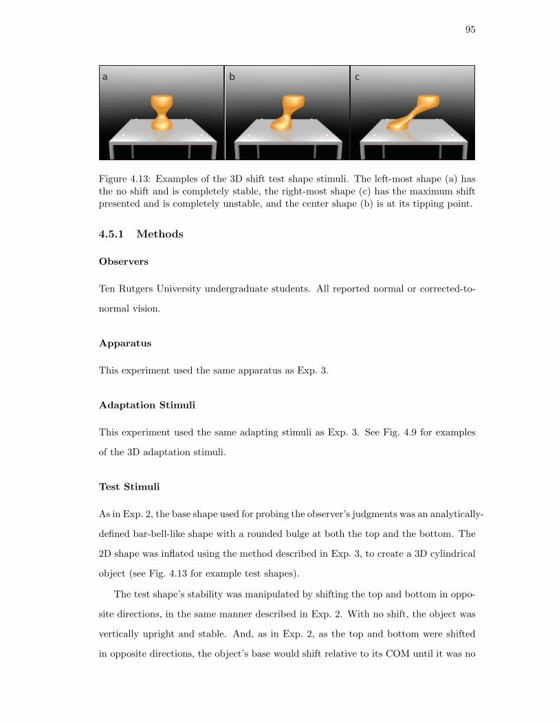
95

a b c

Figure 4.13: Examples of the 3D shift test shape stimuli. The left-most shape (a) hasthe no shift and is completely stable, the right-most shape (c) has the maximum shiftpresented and is completely unstable, and the center shape (b) is at its tipping point.

4.5.1 Methods

Observers

Ten Rutgers University undergraduate students. All reported normal or corrected-to-

normal vision.

Apparatus

This experiment used the same apparatus as Exp. 3.

Adaptation Stimuli

This experiment used the same adapting stimuli as Exp. 3. See Fig. 4.9 for examples

of the 3D adaptation stimuli.

Test Stimuli

As in Exp. 2, the base shape used for probing the observer’s judgments was an analytically-

defined bar-bell-like shape with a rounded bulge at both the top and the bottom. The

2D shape was inflated using the method described in Exp. 3, to create a 3D cylindrical

object (see Fig. 4.13 for example test shapes).

The test shape’s stability was manipulated by shifting the top and bottom in oppo-

site directions, in the same manner described in Exp. 2. With no shift, the object was

vertically upright and stable. And, as in Exp. 2, as the top and bottom were shifted

in opposite directions, the object’s base would shift relative to its COM until it was no

96

longer stable. As in the previous experiments, the shift where the object was equally

likely to stay upright or fall was defined as the tipping point.

Fifty-one test stimuli were generated by with top/bottom shifts ranging from 0 DV A

to 7.42 DV A. The tipping point for these test shapes was 2.98 DV A. The shifts were

converted to a 0 to 0.5 scale, where 0 was no shift (0 DV A) and 0.5 was the maximum

shift presented (7.42 DV A), making the critical lateral shift 0.20 (2.98 DV A). During

the experiment, the top of the test shape was randomly shifted either to the left or the

right.

Design

As in the previous experiments, this design used a yes/no paradigm with four conditions:

a pre-test with no adaptation, the two adaptation conditions counterbalanced across

subjects, and a post-test without adaptation.

The experimental procedure was the same as in Exp. 2.

Stimuli were chosen using the Psi adaptive staircase method so that we could esti-

mate the PSE of the psychometric function for observers’ judgments. In the adaptation

conditions, we used the same top-up procedure to adapt observers to either stable or

unstable shapes as was used in the previous experiments.

4.5.2 Results

The Psi method was used to estimate the observers’ PSEs with 95% confidence intervals.

All 10 observers were biased in the direction predicted by a stability aftereffect, with

5 of the 10 observers having significantly different PSEs for the Stable and Unstable

Adaptation conditions (see Fig. 4.14).

As shown in Fig. 4.15, 8 out of 10 of the observers overestimated the stability on

average while the other 2 underestimated stability, with an average PSE of 0.30, which

is above the physical tipping point of 0.20. As with the results from Exp. 3, on average,

the observers in this experiment had a larger biased to overestimate stability than those

in Exp. 2.

97

æ

æ

æ

æ

æ

æ

æ

æ

æ

æ

æ

æ

æ

æ

æ

æ

æ

æ

æ

æ

-0.2 -0.1 0.1 0.2Shift

2

4

6

8

10

Subject

Blue = Stable Adaptation

Red = Unstable Adaptation

Figure 4.14: PSE results using a 3D shift test shape standardized by removing bias (av-erage PSE for the adaptation conditions). Subjects (y-axis) were sorted by magnitudeof the aftereffect (PSE for Unstable Adaptation - PSE for Stable Adaptation), withindividuals showing the smallest aftereffect at the bottom and those with the largestat the top. Note: Lateral shifts are presented using a 0 (0 DV A) to 0.5 (7.42 DV A)scale.

4.6 Conclusion

We found converging evidence that people adapt to object stability, and exhibit a

“stability aftereffect” when making stability judgments after observing using different

shape manipulations of the test object, such curving the axis and introducing lateral

shift between the top and bottom halves. This visual adaptation is quite robust, causing

aftereffects for both 2D and 3D stereoscopically presented scenes. Stability adaptation

is quite surprising because estimating the stability of an object requires integration of a

number of different aspects – using the object’s shape to estimate COM and inference

of gravitational forces on the object – so judging stability may have been dependent

upon higher level reasoning. However, the presence of the aftereffect argues for a lower

level perceptual representation of object stability.

From a purely physical perspective, it would be surprising for the perceived stability

to be affected by previously observed objects. But it may be possible that our visual

system is tuned to emphasize instability, given the fact that the majority of objects

98

Overestimating StabilityUnderestimating Stability

æ

æ

æ

æ

æ

æ

æ

æ

æ

æ

0.1 0.2 0.3 0.4 0.5Shift

2

4

6

8

10

Subject

Figure 4.15: Bias results for the 3D shift experiment. Subjects (y-axis) have the sameordering as in Fig. 4.14, where individuals showing the smallest aftereffect are at thebottom and those with the largest at the top. Note that the vertical dashed line is thephysical tipping point for this test measure. Note: Lateral shifts are presented using a 0(0 DV A) to 0.5 (7.42 DV A) scale, with the physical tipping point at 0.20 (2.98 DV A).

we observe and interact with are normally in a stable equilibrium. If this were the

case, we would see systematic underestimation of stability if observers are told to judge

whether an object is stable or not and, in fact, this is what Samuel and Kerzel (2011)

found. In our experiments presented here, observers were biased to judge the stability

of test objects “on the safe side” after viewing very stable objects, consistent with the

results of Samuel and Kerzel (2011), however, we also found that the direction of the

bias could be reversed, causing them to judge the stability of probe objects “recklessly”

after adapting to unstable objects.

These results, coupled with the previous results in Cholewiak et al. (2012), suggest

that stability is a physical aspect of shape that is judged along a unitary dimension.

People are able to infer the force of gravity acting upon the shapes and predict whether

the objects will stay upright or fall, regardless of whether they are presented as 2D

silhouettes (Exp. 1 and 2) or as volumetric 3D objects (Exp. 3 and 4). In addition,

observers’ stability judgments are affected regardless of the test shape’s manipulation,

whether the probe’s curvature (Exp. 1 and 3) or the top-bottom shift (Exp. 2 and 4)

were manipulated, meaning that we were not simply observing a curvature or shift

99

aftereffect. Although the visual estimation of object stability is sometimes considered

to be a higher-level judgment, our results suggest that it is a bona fide perceptual

variable that is susceptible to adaptation effects.

This conclusion is consistent with our previous finding, using a stability matching

task, that subjects find it easy and natural to adjust the aspect ratio of one object

so that it is perceived as being equally stable as another, despite the fact that the

two objects have different shapes. Similar to color metamerism, where colors that are

composed of different wavelengths appear the same, shapes with the same perceived

stability would be stability metamers. In Cholewiak et al. (2012), we demonstrated that

observers had no difficulty comparing the stability of 3D shapes (slanted conical frus-

tums and cylinders) and readily estimated stability metamers that could be predicted

using aspects of stability – specifically the minimum critical angles of the two objects.

In the experiments herein, we show that observers were able to estimate the tipping

point, regardless of the underlying shape manipulation, meaning that the manipulated

shapes at their tipping points were stability metamers.

Our results indicated that some judgments of physical attributes, such as object

stability tested here, actually involve unidimensional perceptual variables.

100

Chapter 5

Conclusion

The inference of forces is an ecologically important aspect of visual perception. We use

it to make judgments of physical interactions – including collisions (Scholl & Nakayama,

2002), support relations (Baillargeon & Hanko-Summers, 1990; Baillargeon et al., 1992)

and stability (Barnett-Cowan et al., 2011; Samuel & Kerzel, 2011) – in the service of

future actions. The reported research provides evidence for the visual estimation of

stability, which requires the inference of gravitational forces acting upon objects.

As shown in Chapter 2, observers judgments of an object’s stability are invariant

to the volume of the object and appeared to only be a function of the object’s shape.

This is significant for the representation of the object’s physical parameters, such as

the COM and bounding contour, because it suggests we use an objects shape – rather

than relying on purely retinotopic representations – when making stability judgments.

The critical angle tasks described in Chapter 2 identified a shape-dependent stability

effect, specifically that stability was underestimated for short-and-wide shapes, and

overestimated for tall-and-narrow shapes. This contradicts the assertion by Samuel and

Kerzel (2011) – in the context of 2D shapes – that stability judgments would always

be “on the safe side”. And although there were biases to under and overestimate

the stability of the object, observers were on average close to the physical prediction,

suggesting that they used an physically correct internal model to make their judgments.

When asked to estimate the COM, observers were even closer to the physical predictions.

On the individual level though, observers do not appear to rely on the COM in making

judgments of physical stability. Their COM stability estimates are much less biased

and have a larger effect of aspect ratio.

101

When adding a part to the conical frustums, observers tended on average to down-

weight the influence of the attached part on the object’s physical stability. Although

their perceived influence was often close to the physical influence of the part on overall

stability, there was a tendency to underestimate the part’s contribution and decrease

the perceived influence of the part’s additional mass. This down-weighting is consistent

with a robust-statistics approach to determining the influence of a potentially sepa-

rate part on global shape estimation (Cohen & Singh, 2006; Denisova et al., 2006).

It provides some evidence for part-based representation of shape (versus an unstruc-

tured, template-like account of shape representation, where all points within a shape

are treated equally).

Chapter 3 addressed the question of whether stability is a unitary dimension. Do

people use an “internal scale” of very stable and unstable objects when judging the

stability of other objects (perhaps calibrated to their own perceptual biases)? Moreover,

a potential concern with using the critical angle task (as introduced in Chapter 2) as a

measure of overall stability is that with asymmetric objects, the critical angle is not a

single number, but instead a function of the direction of tilt.

Therefore, the first experiment in Chapter 3 investigated how well observers could

track the critical angle as a function of the direction of skew for asymmetric 3D objects.

We found that observers were quite accurate for most skew directions (as would have

been expected from the critical angle results in Chapter 2). Given that observers’ perfor-

mance for asymmetric objects was established, the subsequent experiments addressed

the idea that if perceived stability were a one dimensional attribute, then observers

should have been able to assign a single value to describe an object’s stability. We

investigated how are the critical angles in different directions combined into a single

estimate of object stability.

This required a separate task that assessed overall stability, so we asked observers to

match different objects’ stabilities and tested to see if there was a predictable relation-

ship between the critical angles of asymmetric shapes and their perceived stabilities.

The results showed that, for most observers, the minimum critical angle was a better

model for their stability estimate than the mean, namely, that the critical angle in the

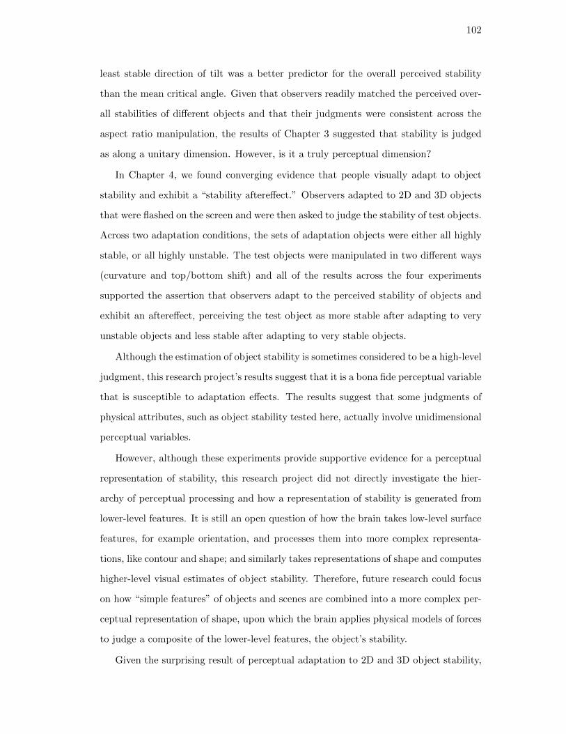
102

least stable direction of tilt was a better predictor for the overall perceived stability

than the mean critical angle. Given that observers readily matched the perceived over-

all stabilities of different objects and that their judgments were consistent across the

aspect ratio manipulation, the results of Chapter 3 suggested that stability is judged

as along a unitary dimension. However, is it a truly perceptual dimension?

In Chapter 4, we found converging evidence that people visually adapt to object

stability and exhibit a “stability aftereffect.” Observers adapted to 2D and 3D objects

that were flashed on the screen and were then asked to judge the stability of test objects.

Across two adaptation conditions, the sets of adaptation objects were either all highly

stable, or all highly unstable. The test objects were manipulated in two different ways

(curvature and top/bottom shift) and all of the results across the four experiments

supported the assertion that observers adapt to the perceived stability of objects and

exhibit an aftereffect, perceiving the test object as more stable after adapting to very

unstable objects and less stable after adapting to very stable objects.

Although the estimation of object stability is sometimes considered to be a high-level

judgment, this research project’s results suggest that it is a bona fide perceptual variable

that is susceptible to adaptation effects. The results suggest that some judgments of

physical attributes, such as object stability tested here, actually involve unidimensional

perceptual variables.

However, although these experiments provide supportive evidence for a perceptual

representation of stability, this research project did not directly investigate the hier-

archy of perceptual processing and how a representation of stability is generated from

lower-level features. It is still an open question of how the brain takes low-level surface

features, for example orientation, and processes them into more complex representa-

tions, like contour and shape; and similarly takes representations of shape and computes

higher-level visual estimates of object stability. Therefore, future research could focus

on how “simple features” of objects and scenes are combined into a more complex per-

ceptual representation of shape, upon which the brain applies physical models of forces

to judge a composite of the lower-level features, the object’s stability.

Given the surprising result of perceptual adaptation to 2D and 3D object stability,

103

it would be important in future studies to examine this phenomenon in greater detail,

especially with respect to the time course of the adaptation. For example: How long

does the adaptation persist? How resistant is it to repeated presentations of the test

stimuli? Given that perceptual adaptation has been shown to exhibit build-up and

decay over time – for example, as demonstrated with motion (Hoffmann, Dorn, & Bach,

1999), visual gratings (Greenlee, Georgeson, Magnussen, & Harris, 1991), audition

(Anstis & Saida, 1985), and chromatic adaptation (Fairchild & Reniff, 1995) – future

experiments investigating the time course of stability adaptation would provide further

evidence for a purely perceptual representation of shape.

104

References

Anderson, B. L., Singh, M., & Fleming, R. (2002). The interpolation of object and sur-

face structure. Cognitive Psychology , 44 , 148–190. doi: 10.1006/cogp.2001.0765

Anstis, S., & Saida, S. (1985). Adaptation to auditory streaming of frequency-

modulated tones. Journal of Experimental Psychology: Human Perception and

Performance, 11 , 257–271. doi: 10.1037/0096-1523.11.3.257

Baillargeon, R., & Hanko-Summers, S. (1990). Is the top object adequately supported

by the bottom object? young infants’ understanding of support relations. Cogni-

tive development , 5 , 29–53. doi: 10.1016/0885-2014(90)90011-H

Baillargeon, R., Needham, A., & DeVos, J. (1992). The development of young infants’

intuitions about support. Early Development and Parenting , 1 , 69–78. doi:

10.1002/edp.2430010203

Barnett-Cowan, M., Fleming, R. W., Singh, M., & Bulthoff, H. H. (2011). Perceived

object stability depends on multisensory estimates of gravity. PLoS ONE , 6 , 1–5.

doi: 10.1371/journal.pone.0019289

Baud-Bovy, G., & Gentaz, E. (2004). The visual localization of the centre of triangles

in young children and adults. Current Psychology Letters, 13 , 2–11.

Baud-Bovy, G., & Soechting, J. (2001). Visual localization of the center of mass

of compact, asymmetric, two-dimensional shapes. Journal of Experimental Psy-

chology: Human Perception and Performance, 27 , 692–706. doi: 10.1037/0096-

1523.27.3.692

Becker, W., & Fuchs, A. F. (1985). Prediction in the oculomotor system: Smooth

pursuit during transient disappearance of a visual target. Experimental Brain

Research, 57 , 562–575. doi: 10.1007/BF00237843

Biederman, I. (1987). Recognition-by-components: A theory of human image under-

standing. Psychological Review , 94 , 115–147. doi: 10.1037/0033-295X.94.2.115

105

Bingham, G. P., & Muchisky, M. M. (1993). Center of mass perception and in-

ertial frames of reference. Perception & Psychophysics, 54 , 617–632. doi:

10.3758/BF03211785

Blum, H. (1967). A transformation for extracting new descriptors of shape. Models for

the perception of speech and visual form, 362–380.

Brainard, D. (1997). The Psychophysics Toolbox. Spatial Vision, 10 , 433–436. doi:

10.1163/156856897X00357

Burr, D. C., Anobile, G., & Turi, M. (2011). Adaptation affects both high and low

(subitized) numbers under conditions of high attentional load. Seeing and Per-

ceiving , 24 , 141–150. doi: 10.1163/187847511X570097

Burr, D. C., & Ross, H. (2002). Direct evidence that “speedlines” influence motion

mechanisms. The Journal of Neuroscience, 22 , 8661–8664.

Burr, D. C., & Ross, H. (2008). A visual sense of number. Current Biology , 18 , 1–4.

doi: 10.1016/j.cub.2008.02.052

Carello, C., Fitzpatrick, P., Domaniewicz, I., Chan, T.-C., & Turvey, M. T. (1992).

Effortful touch with minimal movement. Journal of Experimental Psychology: Hu-

man Perception and Performance, 18 , 290-302. doi: 10.1037/0096-1523.18.1.290

Cholewiak, S. A., Fleming, R., & Singh, M. (2011). Perception of physical stability

of asymmetrical three-dimensional objects [abstract]. Journal of Vision. doi:

10.1167/11.11.44

Cholewiak, S. A., Fleming, R. W., & Singh, M. (2012). Perception of the physical

stability of asymmetrical three-dimensional objects. Journal of Vision, Under

Review.

Cholewiak, S. A., Singh, M., Fleming, R., & Pastakia, B. (2010). The perception of

physical stability of 3d objects: The role of parts [abstract]. Journal of Vision,

10 , 77. doi: 10.1167/10.7.77

Cohen, E. H., & Singh, M. (2006). Perceived orientation of complex shape reflects

graded part decomposition. Journal of Vision, 6 , 805–821. doi: 10.1167/6.8.4

Cooper, P. R., Birnbaum, L. A., & Brand, M. E. (1995). Causal scene under-

standing. Computer vision and image understanding , 62 (2), 215–231. doi:

106

10.1006/cviu.1995.1051

Dan, B. (2007). Balancing bricks . . . again . . . Retrieved from

http://www.flickr.com/photos/rocker/2068407802/

Dempsey, J. (2008). Stone age jenga. Retrieved from

http://www.flickr.com/photos/stonemason/2545658903/

Denisova, K., Singh, M., & Kowler, E. (2006). The role of part structure in the per-

ceptual localization of a shape. Perception, 35 , 1073–1087. doi: 10.1068/p5518

Dragoi, V., Sharma, J., Miller, E. K., & Sur, M. (2002). Dynamics of neuronal sensi-

tivity in visual cortex and local feature discrimination. Nature Neuroscience, 5 ,

883–891. doi: 10.1038/nn900

Dragoi, V., Sharma, J., & Sur, M. (2000). Adaptation-induced plasticity of orienta-

tion tuning in adult visual cortex. Neuron, 28 , 287–298. doi: 10.1016/S0896-

6273(00)00103-3

Fairchild, M. D., & Reniff, L. (1995). Time course of chromatic adaptation for color-

appearance judgments. Journal of the Optical Society of America, 12 , 824–833.

doi: 10.1364/JOSAA.12.000824

Feldman, J., & Singh, M. (2006). Bayesian estimation of the shape skeleton.

Proceedings of the National Academy of Sciences, 107 , 18014–18019. doi:

10.1073/pnas.0608811103

Freyd, J. J. (1983). The mental representation of movement when static stimuli are

viewed. Perception & Psychophysics, 33 , 575–581. doi: 10.3758/BF03202940

Freyd, J. J., & Finke, R. A. (1984). Representational momentum. Journal of Ex-

perimental Psychology: Learning, Memory, and Cognition, 10 , 126–132. doi:

10.1037/0278-7393.10.1.126

Freyd, J. J., & Jones, K. T. (1994). Representational momentum for a spiral path.

Journal of Experimental Psychology: Learning, Memory, and Cognition, 20 , 968–

976. doi: 10.1037/0278-7393.20.4.968

Freyd, J. J., Pantzer, T. M., & Cheng, J. L. (1988). Representing statics as forces in

equilibrium. Journal of Experimental Psychology: General , 117 , 395–407. doi:

10.1037/0096-3445.117.4.395

107

Friedman, W. J. (2002). Arrows of time in infancy: The representation

of temporal-causal invariances. Cognitive Psychology , 44 , 252–296. doi:

10.1006/cogp.2001.0768

Geilser, W. S. (1999). Motion streaks provide a spatial code for motion direction.

Nature, 400 , 65–69. doi: 10.1038/21886

Gibson, J. J. (1954). The visual perception of objective motion and subjective move-

ment. Psychological Review , 61 , 304–314. doi: 10.1037/h0061885

Graf, E. W., Warren, P. A., & Maloney, L. T. (1995). Explicit estimation of visual

uncertainty in human motion perception. Vision Research, 45 , 3050–3059. doi:

10.1016/j.visres.2005.08.007

Greenlee, M. W., Georgeson, M. A., Magnussen, S., & Harris, J. P. (1991). The

time course of adaptation to spatialcontrast. Vision Research, 31 , 223–236. doi:

10.1016/0042-6989(91)90113-J

Hamrick, J., Battaglia, P. W., & Tenenbaum, J. B. (2011). Internal physics models

guide probabilistic judgments about object dynamics. In Proceedings of the 33rd

cognitive science society annual conference.

Harris, C. S. (1963). Adaptation to displaced vision: Visual, motor, or proprioceptive

change? Science, 140 , 812–813. doi: 10.1126/science.140.3568.812

Hoffmann, M., Dorn, T. J., & Bach, M. (1999). Time course of motion adaptation:

Motion-onset visual evoked potentials and subjective estimates. Vision Research,

39 , 437–444. doi: 10.1016/S0042-6989(98)00186-2

Hong, J., & Papathomas, T. V. (2006). Influences of attention on auditory after-

effects following purely visual adaptation. Spatial Vision, 19 , 569–580. doi:

10.1163/156856806779194044

Humphrey, G. K., & Jolicoeur, P. (1993). An examination of the effects of axis fore-

shortening, monocular depth cues, and visual field on object identification. The

Quarterly Journal of Experimental Psychology, Section A: Human Experimental

Psychology , 46 , 137–159. doi: 10.1080/14640749308401070

Kaiser, M. K., Proffitt, D. R., & Anderson, K. (1985). Judgments of natural and

anomalous trajectories in the presence and absence of motion. Learning, Memory,

108

and Cognition, 11 , 795–803. doi: 10.1037/0278-7393.11.1-4.795

Kaiser, M. K., Proffitt, D. R., Whelan, S. M., & Hecht, H. (1992). Influence of animation

on dynamical judgments. Journal of Experimental Psychology , 18 , 669–690. doi:

10.1037/0096-1523.18.3.669

Kim, I. K., & Spelke, E. S. (1992). Infants’ sensitivity to effects of gravity on visi-

ble object motion. Journal of Experimental Psychology: Human Perception and

Performance, 18 , 385–393. doi: 10.1037/0096-1523.18.2.385

Kim, S.-H., Feldman, J., & Singh, M. (2012). Curved apparent motion initiated by a

causal launch. Psychological Science, In Press.

Kingdom, F. A. A., & Prins, N. (2010). Psychophysics: A practical introduction.

London: Academic Press.

Kleiner, M., Brainard, D., & Pelli, D. (2007). What’s new in psychtoolbox-3? Percep-

tion, 36 , ECVP Abstract Supplement.

Koenderink, J. J. (1998). Pictorial relief. Philosophical Transactions of the Royal

Society of London Series A, 356 , 1071–1086. doi: 10.1098/rsta.1998.0211

Koenderink, J. J., van Doorn, A. J., & Kappers, A. M. L. (1992). Surface perception in

pictures. Perception & Psychophysics, 52 , 487–496. doi: 10.3758/BF03206710

Kohn, A., & Movshon, J. A. (2003). Neuronal adaptation to visual motion in area mt

of the macaque. Neuron, 39 , 681–691. doi: 10.1016/S0896-6273(03)00438-0

Kohn, A., & Movshon, J. A. (2004). Adaptation changes the direction tuning of

macaque mt neurons. Nature Neuroscience, 7 , 764–772. doi: 10.1038/nn1267

Kontsevich, L. L., & Tyler, C. W. (1999). Bayesian adaptive estimation of psychome-

tric slope and threshold. Vision Research, 39 , 2729–2737. doi: 10.1016/S0042-

6989(98)00285-5

Korte, A. (1915). Kinematoskopische untersuchungen [Kinematoscope investigations].

Zeitschrift fur Psychologie, 72 , 193–296.

Lasseter, J. (1987). Principles of traditional animation applied to 3d computer ani-

mation. In Siggraph ’87 proceedings of the 14th annual conference on computer

graphics and interactive techniques (Vol. 21, pp. 35–44). New York, NY: ACM.

doi: 10.1145/37401.37407

109

Lawson, R., & Humphreys, G. W. (1998). View-specific effects of depth rotation and

foreshortening on the initial recognition and priming of familiar objects. Percep-

tion & Psychophysics, 60 , 1052–1066. doi: 10.3758/BF03211939

Lederman, S. J., Ganeshan, S. R., & Ellis, R. E. (1996). Effortful touch with minimum

movement: Revisited. Journal of Experimental Psychology: Human Perception

and Performance, 22 , 851-868. doi: 10.1037/0096-1523.22.4.851

Marr, D. (1982). Vision. San Francisco, CA: W H Freeman.

Marr, D., & Nishihara, H. K. (1978). Representation and recognition of the spatial orga-

nization of three-dimensional shapes. Proceedings of the Royal Society of London,

Series B, Biological Sciences, 200 , 269–294. doi: 10.1098/rspb.1978.0020

McCloskey, M. (1983a). Intuitive physics. Scientific American, 248 , 122–130. doi:

10.1038/scientificamerican0483-122

McCloskey, M. (1983b). Naive theories of motion. In D. Gentner & A. L. Stevens (Eds.),

Mental models (pp. 299–324). Hillsdale, NJ: Lawrence Erlbaum Associates, Inc.

McCloskey, M., Caramazza, A., & Green, B. (1980). Curvilinear motion in the absence

of external forces: Naive beliefs about the motion of objects. Science, 210 , 1139–

1141. doi: 10.1126/science.210.4474.1139

McCloskey, M., & Kohl, D. (1983). Naive physics: The curvilinear impetus principle and

its role in interactions with moving objects. Journal of Experimental Psychology:

Learning, Memory, and Cognition, 9 , 146–156. doi: 10.1037/0278-7393.9.1.146

McCloskey, M., Washburn, A., & Felch, L. (1983). Intuitive physics: The straight-down

belief and its origin. Journal of Experimental Psychology: Learning, Memory, and

Cognition, 9 , 636–649. doi: 10.1037/0278-7393.9.4.636

McIntyre, J., Zago, M., Berthoz, A., & Lacquaniti, F. (2001). Does the brain model

Newton’s laws? Nature Neuroscience, 4 , 693–694. doi: 10.1038/89477

Melcher, D., & Kowler, E. (1999). Shapes, surfaces and saccades. Vision Research, 39 ,

2929–2946. doi: 10.1016/S0042-6989(99)00029-2

Morales, T. (2009). Amputee aims to scale new peaks. Retrieved from

http://www.cbsnews.com/stories/2003/05/06/earlyshow/living/

main552498.shtml

110

Morgan, M. J., Hole, G. J., & Glennerster, A. (1990). Biases and sensitivities in geomet-

rical illusions. Vision Research, 30 , 1793–1810. doi: 10.1016/0042-6989(90)90160-

M

Moscatelli, A., Polito, L., & Lacquaniti, F. (2011). Time perception of action pho-

tographs is more precise than that of still photographs. Experimental Brain Re-

search, 210 , 25–32. doi: 10.1007/s00221-011-2598-y

Needham, A., & Baillargeon, R. (1993). Intuitions about support in 4.5-month-old

infants. Cognition, 47 , 121–148. doi: 10.1016/0010-0277(93)90002-D

Newman, G. E., Choi, H., Wynn, K., & Scholl, B. J. (2008). The origins of causal per-

ception: Evidence from postdictive processing in infancy. Cognitive Psychology ,

57 , 262–291. doi: 10.1016/j.cogpsych.2008.02.003

Pavel, M., Cunningham, H., & Stone, V. (1992). Extrapolation of linear motion. Vision

Research, 32 , 2177–2186. doi: 10.1016/0042-6989(92)90078-W

Pelli, D. G. (1997). The VideoToolbox software for visual psychophysics:

Transforming numbers into movies. Spatial Vision, 10 , 437–442. doi:

10.1163/156856897X00366

Proffitt, D. R., & Gilden, D. L. (1989). Understanding natural dynamics. Journal of

Experimental Psychology , 15 , 384–393. doi: 10.1037/0096-1523.15.2.384

Roncato, S., & Rumiati, R. (1986). Naive statics: Current misconceptions on equilib-

rium. Journal of Experimental Psychology: Learning, Memory, and Cognition,

12 , 361–377. doi: 10.1037/0278-7393.12.3.361

Samuel, F., & Kerzel, D. (2011). Is this object balanced or unbalanced? Judgments

are on the safe side. Journal of Experimental Psychology: Human Perception and

Performance, 37 , 529–538. doi: 10.1037/a0018732

Scholl, B. J., & Nakayama, K. (2002). Causal capture: Contextual effects on the per-

ception of collision events. Psychological Science, 13 , 493–498. doi: 10.1111/1467-

9280.00487

Scholl, B. J., & Pylyshyn, Z. W. (1999). Tracking multiple items through occlu-

sion: Clues to visual objecthood. Cognitive Psychology , 38 , 259–290. doi:

10.1006/cogp.1998.0698

111

Shah, S., Fulvio, J., & Singh, M. (2012). Perceptual decisions in the visual extrapolation

of curved motion trajectories. Journal of Vision, Under Review.

Singer, G., & Day, R. H. (1966a). The effects of spatial judgments on the perceptual

aftereffect resulting from prismatically transformed vision. Australian Journal of

Psychology , 18 , 63–70. doi: 10.1080/00049536608255717

Singer, G., & Day, R. H. (1966b). Spatial adaptation and aftereffect with optically

transformed vision: Effects of active and passive responding and the relationship

between test and exposure responses. Journal of Experimental Psychology , 71 ,

725–731. doi: 10.1037/h0023089

Singh, M. (2004). Modal and amodal completion generate different shapes. Psycholog-

ical Science, 15 , 454–459. doi: 10.1111/j.0956-7976.2004.00701.x

Tootell, R. B. ., Reppas, J. B., Dale, A. M., Look, R. B., Sereno, M. I., Malach, R.,

. . . Rosen, B. R. (1995). Visual motion aftereffect in human cortical area MT

revealed by functional magnetic resonance imaging. Nature, 375 , 139–141. doi:

10.1038/375139a0

Verghese, P., & McKee, S. P. (2002). Predicting future motion. Journal of Vision, 2 ,

513–523. doi: 1167/2.5.5

Vishwanath, D., & Kowler, E. (2003). Localization of shapes: eye movements and

perception compared. Vision Research, 43 , 1637–1653. doi: 10.1016/S0042-

6989(03)00168-8

Vishwanath, D., & Kowler, E. (2004). Saccadic localization in the presence of cues to

three-dimensional shape. Journal of Vision, 4 , 445–458. doi: 10.1167/4.6.4

Wertheimer, M. (1912). Experimentelle Studien uber das Sehen von Bewegung. [Ex-

periments on the perception of motion]. Zeitschrift fur Psychologie, 61 , 161-265.

White, B. Y. (1983). Sources of difficulty in understanding newtonian dynamics.

Cognitive Science, 7 , 41–65. doi: 10.1207/s15516709cog0701 2

Winawer, J., Huk, A. C., & Boroditsky, L. (2008). A motion aftereffect from

still photographs depicting motion. Psychological Science, 19 , 276–283. doi:

10.1111/j.1467-9280.2008.02080.x

112

Zago, M., & Lacquaniti, F. (2005). Visual perception and interception of falling ob-

jects: A review of evidence for an internal model of gravity. Journal of Neural

Engineering , 2 , 198–208. doi: 10.1088/1741-2560/2/3/S04

Zollinger, D. (2008). Tbilisi (georgia) - former transport ministry. Retrieved from

http://www.flickr.com/photos/danielzolli/2497272343/