The Theoretic Research of Tachyons with Real Mass: …article.sciencepublishinggroup.com/pdf/10.11648.j.ijhep.20180501... · International Journal of High Energy ... The Theoretic

International Journal of High Energy Physics 2018; 5(1): 23-43

http://www.sciencepublishinggroup.com/j/ijhep

doi: 10.11648/j.ijhep.20180501.14

ISSN: 2376-7405 (Print); ISSN: 2376-7448 (Online)

The Theoretic Research of Tachyons with Real Mass: Tachyon Transformation Matrix, Tachyon Oscillations, and Measuring Tachyon Velocity

Zoran Bozidar Todorovic

Faculty of Sciences, Department of Physics, the University of Pristina, Kosovska Mitrovica, Serbia

Email address:

To cite this article: Zoran Bozidar Todorovic. The Theoretic Research of Tachyons with Real Mass: Tachyon Transformation Matrix, Tachyon Oscillations, and

Measuring Tachyon Velocity. International Journal of High Energy Physics. Vol. 5, No. 1, 2018, pp. 23-43.

doi: 10.11648/j.ijhep.20180501.14

Received: April 23, 2018; Accepted: May 17, 2018; Published: June 11, 2018

Abstract: In this paper, a theoretical approach has been used in order to present the physical characteristics of tachyons with

real mass. The procedure of the transfer from the Einstein’s physics into the world of superluminal particles has been given. In

addition, the tachyon transformation matrix has been constructed using the principle of correspondence between these two

physics. With the usage of the tachyon matrix, it has been shown how length contraction and time dilatation are calculated in

the tachyons case. A particular attention has been devoted to measuring the velocity of tachyons and their potential flavor

oscillations since it should be kept in mind that there is no rest reference frame attached to tachyon world lines and, in that

sense, special relativity does not treat tachyons on the same footing as particles that are slower than light. It has been

demonstrated, using the Lorentz transformation matrix, that it is impossible to measure the velocities above the speed of light

with the method of measuring time of flight in laboratories over a certain distance. It has been particularly disclosed that

tachyons as isolated particles each on its own could not exist in nature, and if they did exist, they would always appear united

with other tachyon types. Owing to that tachyon characteristic, obtained by theoretical consideration, it has been concluded

that tachyons, rather than neutrinos as subluminal particles, could comply with the definition for the occurrence of the

oscillation phenomena between different tachyon types. Furthermore, the analysis of the velocity of emitted neutrinos during

the explosion of Supernova SN1987A has been conducted in the spirit of the proposed theory, where it has been demonstrated

that it is possible to measure even superluminal velocities with the usage of that measuring method.

Keywords: Special Relativity, Leptons, Tachyons, Neutrino Mass and Mixing

1. Introduction

At first, after the discovery of neutrinos, it was considered

that they possess no mass, which was the reason of claims

that their velocity coincides with the speed of light. Further

development of the physics of neutrinos experimentally

established their feature of turning from one flavor state into

another flavor state and vice versa, in the process known as

the neutrino oscillation [1-3].

Neutrino oscillation confirmed that neutrinos possess mass

and that changed the understanding of their velocity. Mass no

longer equals zero, it exists, although it has a rather low, still

undefined value. Due to the possession of such mass,

contemporary physics considers that the neutrino velocity

would be a little lower than the speed of light. Whether the

existence of mass is the main reason for such a neutrino

velocity or there is something else in question, remains to be

seen in further consideration of the proposed theory of

superluminal particles.

All measurements of the neutrino velocity conducted in

laboratories, regardless of the location of those

measurements, showed almost identical results [4-8], the

value of which is a little below the speed of light. Such a

small deviation from the speed of light would be attributed to

their low mass that is still a mysterious and unresolved value

in physics.

G. Feinberg was one of the first to propose the theory of

particles faster than light as early as in 1967. [9]. Since he

24 Zoran Bozidar Todorovic: The Theoretic Research of Tachyons with Real Mass: Tachyon Transformation

Matrix, Tachyon Oscillations, and Measuring Tachyon Velocity

based his theory on the grounds of Einstein’s formula for the

energy of a particle, which was well known in physics, it

resulted in the fact that the mass of a particle which they

called tachyon had to be an imaginary value. It was simply

computed by taking a square root of a negative number.

Thus, the basis of all the previous theories in physics related

to a tachyon as a theoretically postulated particle which

moved faster than light, but which possessed imaginary mass.

Contrary to previous theories, this paper underlines that

there is an essential difference between the name of particles

faster than light which was introduced in the previous

theories and a tachyon which is the subject of the research in

this work.

Namely, in previous theories, a tachyon was observed as a

particle with imaginary mass, while, in the given theoretical

model of this work, a tachyon is considered as a particle

which possesses real mass.

That is why it must be stated that a tachyon as a particle

with imaginary mass does not belong to the real world of

particles.

That is actually the only reason to search for a possible

mathematical model which would describe a tachyon as a

particle with real mass, and give it a chance to join the world

of real particles. Such a mathematical model had to arise

from Einstein’s energy relation where the limit determined by

the speed of light would be easily skipped and, thus, a

domain defined by the speed of motion would be extended to

infinite velocity.

Additionally, it is generally known that in today’s physics,

tachyons represent only hypothetical particles which have not

been measured in real experiments, so far.

However, regardless of such a status of a tachyon in

today’s physics, this paper considers, for now, that there is at

least a theoretical possibility for the existence of a tachyon.

According to the above, the similar attitude states that

there are some suggestions given in the reference [10, 16],

where it is considered that neutrinos could be tachyons.

In order to make a comparison between the previous

theories and the one suggested in this work, it will be shown

how to make a transition from Einstein’s physics, defined by

the top-limit speed being equal to the speed of light and the

physics of tachyons with real mass, where the domain of

speed is extended from the speed of light to an infinite value.

A special chapter is dedicated to the defining of spacetime

fabric and its application in the definition of the velocity of

tachyons.

The main idea and the procedure of defining energy

function of a tachyon with real mass are also given. At that

point, the transition from Einstein’s physics to the physics of

superluminal particles is presented.

By defining the energy function of a tachyon with real

mass, there is a possibility to introduce not one, but two

energy functions, which will be done in the next section.

The contents of this paper emphasize some chapters

related to the construction of the theoretic model of

superluminal particles, tachyon transformation matrix and its

application. A particular attention has been devoted to the

theoretical model of oscillations of superluminal particles in

the domain of the velocities approximate to the speed of

light. It has been shown that it is impossible to measure

velocities higher that the speed of light in certain

circumstances. A particular attention has been devoted to the

method of measuring the velocity of neutrinos in

contemporary laboratories, as well as to the analysis of the

results of the arrival of neutrinos and photons in the

laboratories on the Earth emitted during the explosion of

Supernova SN1987A.

2. The Transition from Einstein's Physics

to the World of Superluminal Physics

The transition from Einstein's physics to the world of

superluminal physics is extremely simple. To illustrate that, it

is necessary to start from the squared version of Einstein's

energy equation

( ) ( )222 2E pc mc= + (1)

where

( )

2

2

;

1;

1

p m v E m c

v c

v c

γ γ

γ

= =

= <−

(2)

represents the particle momentum, and m is the rest mass

particle, while

c − represents the speed of light

As it is known, this equation can be represented in the

form of a right-angled triangle. One of the catheti of such an

energy triangle is ( )pc and the other is ( )2mc , whilst the

energy of the particle E represents the hypotenuse.

To move to the world of tachyons − superluminal particles,

only the second cathetus needs to be modified, i.e. to be

written in the following form

( ) ( )2mc mcU→

where U represents the coordinate speed of the superluminal

particle defined by

; , ,ii

dXU c i x y z

dt= > =

The cathetus ( )pc does not change. The other one is

modified, but in such a way that the observed mass in the

domain ( )0,c Em becomes m

with the transition into the domain ( )( ), 1c c δ+

( ) ( )2Em c mcU= (3)

International Journal of High Energy Physics 2018; 5(1): 23-43 25

The mass Em which was primarily the rest mass now

becomes the tachyon mass m , mutually connected by the

relation

E

Um m

c= (4)

With such a modification, in a single step, the Einstein's

relativistic energy formula provides the energy formula for a

superluminal particle

( ) ( )2 22

2 2 2

E pc mcU

E c p m U

= + →

= + (5)

where m − represents the mass of the superluminal particle

with minimal speed, which is close to the speed of light but

from the top side, and, thereby, it can be explicitly

represented by the formula [9]

( )2 4

21 1 ; 1

2

m cU c c

Eδ δ

= + = + <<

(6)

Equation (5) represents a right-angled energy triangle with

the hypotenuse E and the catheti ( )pc and ( )mcU .

3. Describing Tachyons Using four

Vectors

3.1. Space-like Interval

There is a reference frame where the two events are

observed occurring at the same time, but there is not a

reference frame in which the two events can occur in the

same spatial location. For these space-like event pairs with

the positive space-time interval

( )2 0S > , the measuring of space-like separation provides

the proper distance

2 2 2 2S S r c t∆ = = ∆ − ∆ (7)

3.2. Time-like Interval

The measuring of a time-like space-time interval is

described by the proper time

2 2 22

2 21

1;

U t Ut t

c c

t U c

τ ∆∆ = − ∆ = ∆ −

= ∆ >Γ

(8)

Thus, it results in

t τ∆ = Γ∆ (9)

And, the definition of the tachyon factor Γ , from here, is

2

2

1

1

t

U

c

τ∆ = Γ =∆

−

(10)

3.3. Definition of the Tachyon Velocity

Proper velocity is defined by

dXw

dτ= (11)

The tachyon’s factor is

2 2

1

1

dt

d U cτΓ = =

− (12)

And the coordinate velocity

dXU

dt= (13)

that describes an object’s rate of motion.

Tachyon four-velocity

The four-coordinate function

( )

0

1

2

3

X ct

X xX

yX

zX

α τ

= =

(14)

defining a tachyon world line, a real function of a variable τ

can be simply differentiated in the usual calculus. The

tangent will be denoted vector of the tachyon world line

( )X α τ is a four-dimensional vector called four-velocity,

; 0,1,2,3.dX

Ud

αα α

τ= = (15)

The relationship between the time t and the coordinate

time 0X is given by

0X ct= (16)

Taking the derivatives with respect to the proper timeτ ,

the 0U velocity is found

( ) ( )0 d ct dt dU ct c

d d dtτ τ= = = Γ (17)

Using the chain rule for 1, 2,3,α = it leads to

( )1 2 3

;

; ;

1,2,3

X

d XdX dtU U

d d dt

X x X y X z

α

ααα

τ τ

α

= = = Γ

= = ==

(18)



Therefore, it results in

0

1

2

3

2 2 2 ; 0,1, 2,3.

x

y

z

x y z

U c

UU cU

U UU

UU

U U U U

α

α

Γ Γ Γ = = = Γ Γ

Γ

= + + =

(19)

Comment.

In the theory of relativity, the world line is the fabric of the

spacetime defined by a similar structural relation

0

11

22

33

ctX

XXx

XX

XX

α

= =

(20)

This structure is a foundation of the theory of relativity;

the same as the (14) is the foundation of the tachyon theory.

In order to differentiate them, they cannot be denoted with

the same letters. Proper distance is the same in both

structures, but there is the difference in the time component.

Therefore, the tachyon structure will be denoted as

0

11

22

33

T

T

ctX

XX ctx

XXX

XX

α

= = →

(21)

Thus, in the theory of relativity, the time component is:

0X ct= (22)

while for a tachyon it is expressed as

0TX ct= (23)

And, that presents the essential difference between these

two theories. This could mean that the value for the measured

time in the tachyon laboratory does not match the measured

time in the classic laboratory of relativistic physics. And, that

means that if classic laboratory measured the time of flight of

tachyons, then the obtained result would not describe its real

state.

3.4. Tachyon Four-momentum

For a massive particle, the four- momentum is given by the

particle’s invariant mass m multiplied by the particle’s

velocity

0

2 2 2

xx

yy

zz

x y z

m cP

m UPP mU

m UP

m UP

m c

m U

p m U U U m U

α α

Γ Γ = = = Γ

Γ

Γ = Γ

= Γ + + = Γ

(24)

Therefore, this relation provides the momentum of the

superluminal particle

2 2 1

mUp m U

U c= Γ =

− (25)

and the connection with energy

2 2 2

22

2 21

��E c p m U pU

mUm U

U c

= + =

= Γ =−

(26)

On the basis of the equation (26), its other equivalent form

is obtained

22 2 2U

E p m cc

= − (27)

4. Klein-Gordon Equation

The proceeding will be carried out as it was made for the

special theory of relativity. Thus, it is started with the identity

from the tachyon theory describing the energy [10].

2 42 2 2 2 2 4

2

U UE p m c p m U

c c= − = − (28)

Then, just inserting the quantum mechanical operators for

momentum and energy yield the equation

24

2 4

2ℏ ℏ

Ui i m U

t xc

∂ ∂ = − − ∂ ∂ (29)

However, this equation has no sense, because differential

equation cannot be evaluated while under the square root

sign. In addition, this equation as it stands, instead begins

with the square of the above identity (28), i.e.

42 2 2 4

2

UE p m U

c= − (30)

which when quantized gives


2 242 4

2ℏ ℏ

Ui i m U

t xc

∂ ∂ Ψ = − Ψ − Ψ ∂ ∂ (31)

and by simplifying, this equation becomes

2 4 2 2 4

2 2 2 20

ℏ

U m U

t c x

∂ ∂Ψ − Ψ − Ψ =∂ ∂

(32)

Free particle solutions

The Klein-Gordon equation for a free particle can be

written as equation (32). We look for plane wave solutions of

the form

( ) ( )

( ) ( )

, exp

exp exp

∓ℏ

∓

ix t px Et

i kx t iω φ

Ψ = ±

= ± =

(33)

For some constant angular frequency Rω ∈ and wave

number 3k R∈ , substitution gives the dispersion relation

4 2 422

2 2ℏ

U m Uk

cω− + = (34)

which represents the equation which satisfies the wave

equation (32). Energy and momentum are seen to be

proportional the ω and �k

��ℏ ℏp i k= Ψ − ∇ Ψ = (35)

ℏ ℏE it

ω∂= Ψ Ψ =∂

(36)

Therefore, dispersion relation is just the energy function of

a tachyonic particle:

( )

42 2 2 4

2

42 2 2

2

UE p m U

c

Up m c

c

= −

= − (37)

For the case of the independence of time, i.e., when is

0t

∂ Ψ =∂

Klein-Gordon equation reduces to the equation

4 2 2 4

2 2 20

ℏ

U m U

c x

∂ + Ψ = ∂ (38)

i.e.

2 2 2

2 20

ℏ

m c

x

∂ + Ψ = ∂ (39)

Also, and in that case one looks for plane wave solutions

of the form

( ) ( )exp expℏ

ix px ikx

Ψ = =

(40)

where the square of a wave number is

2 22

2ℏ

m ck = (41)

And the particle momentum is

ℏp k mc= ± = ± (42)

This momentum represents tachyon when its velocity is

[11]

( )1 ; 12

c EU c n n

mcδ δ

δ= + ≈ = >> (43)

Taking into account (40) and (42), wave function can be

written in the form:

( ) ( )exp expℏ

mcx i x ikx

Ψ = ± = ±

(44)

where the sign “plus” is in relation to tachyons, and sign

“minus” with antitachyons, and it is apparent that the particle

is moving along the x-axis.

5. Tachyonic Transformation Matrix

Apart from the procedure given in [8], a tachyon matrix

will be derived here using the principle of correspondence

between the theory of relativity and the theory of

superluminal particles. Entering a contemporary laboratory

from its tachyon world, a superluminal particle retains its

energy and impulse. We have seen that, owing to the different

domain of velocities ( )0,c it would ostensibly change its

mass (4). And, if it moves close to the speed of light from the

upper side, then its measured mass in a classic laboratory

would be ostensibly higher for the amount1 δ+ . Therefore,

( )1Em m δ= + (45)

To this relation, it is also associated:

The impulse equality

Em v m Uγ = Γ (46)

The energy equality

2 2Em c m Uγ = Γ (47)

On the basis of (45, 46, and 47), the connection among the

members of transformation matrices is obtained:



; 1v

cγ γβ β= = Γ < (48)

; 1= Γ >T Tγ β β (49)

On the basis of the relations (48) and (49), the Lorentz

matrix transforms into tachyon matrix

T

T

L T

U

c

U

c

βγ γββγβ γ

Γ −Γ− = → = −Γ Γ−

Γ −Γ = −Γ Γ

(50)

5.1. Characteristics of a Tachyon Matrix

A tachyon matrix is an orthogonal matrix with the

determinant equaling one:

1

det det

det det 1

T

T

T

T

T

T

ββ

ββ

−

Γ −Γ = −Γ Γ

Γ Γ = = = Γ Γ

(51)

In relation to Minkowski space-time metric, the following

relations can be shown:

( )

1

11 1 1

1

1

T

T

TT I

TgT T gT g

T gT T gT g

gTg T

gT g T

−

−− − −

−

−

=

= =

= =

=

=

(52)

where

1 0 0 0

0 1 0 0

0 0 1 0

0 0 0 1

g

− = −

−

(53)

Minkowski space-time metric and

1 0lim lim

0 1U U

U

cT

U

c

→∞ →∞

Γ −Γ = = −Γ Γ

5.2. Four-momentum Invariance

For the particle moving along x-direction, starting from

(24) and applying the tachyon transformation matrix in the 1S and 2S inertial reference frames, the following can be

written

1 2

1 1 2 2

U

m c m cc

m U m UU

c

Γ −Γ Γ Γ = Γ Γ −Γ Γ

(54)

From this, one gets

( )

1 2 2 2

1 1 2 2 2

1 22 2

;

;

1

Um c m c m U

c

Um U m U m c

c

U c−

Γ = Γ Γ − Γ Γ

Γ = Γ Γ − Γ Γ

Γ = −

(55)

( ) ( )1 2 1 22 2 2 2

1 1 2 21 ; 1U c U c− −

Γ = − Γ = −

Four-momentum invariant quantity is obtained with the

following process:

( )22 2 2 2 2 21 1 1 2 2 2

22 2

2 2 2

m c m U m U m U

Um U m c m c

c

Γ − Γ = ΓΓ − ΓΓ

− ΓΓ − ΓΓ = −

(56)

Also, using Minkowski space-time metric, one gets the

same invariant quantity

22 2 2 2 2 2 2 2 2

2

2 2

1 0 0 0

0 1 0 0

0 0 1 0

0 0 0 1

1

x x

y y

z z

m c m c

m U m U

m U m U

m U m U

Um c m U m c

c

m c

+Γ Γ Γ Γ− Γ Γ− −Γ Γ

= Γ − Γ = Γ −

= −

(57)

5.3. Spacetime Fabric

For the tachyon energy (26), spacetime fabric is defined

Tct

X

(58)

where Tct represents a time component and

x

X y

z

=

is a space coordinate. In the theory of relativity, spacetime

fabric is defined with the matrix


Ect

X

(59)

where Ect is a time component. Thus, as it can be seen, the

essential difference between (58) and (59) lies in different

time components. These components depend on the

laboratory in which the measurements are conducted. In a

tachyon laboratory, the measured time is Tt , whereas in a

classic contemporary laboratory, it is Et and it is usually

labelled as t . The difference between these two times is

particularly emphasized, because if there was no difference in

time component, there would be no difference between the

theory of relativity and the tachyon theory that is proposed

here.

Thus, officially, as far as it is known in contemporary

physics, there is neither the physics of faster-than-light

particles with real mass nor there is a laboratory for their

potential detection. If, by chance, a contact with such

particles existed in a classic laboratory, without knowing they

were superluminal, the misinterpretation of some of their

physical features could occur. Such interpretation would

happen because the two times in (58) and (59) are connected

by the relation [11]

( )2; 1

1

ET

tt δ

δ= <<

+ (60)

It is useful to remember where this relation originates

from. The travelled distance X is defined as proper distance

for both velocity domains and it equals the product of proper

velocities and proper times:

( )

( )

1

1

E E E E E E

T T T T

X w v t v t

w U t Ut

τ γγ

τ

= = =

= = Γ = Γ

(61)

If one switches to the domain of velocities below the light

barrier, which is the domain that belongs to classic

laboratories that observe the particles that subject to the laws

of classic and relativistic physics, then it is inevitable to have

the change of the spacetime structure, as shown below with

an arrow

T Ect ct

X X

→

The travelled distance X remains unchanged, while there is

a change in the time component: T Ect ct→ . These relations

become more apparent if transformed in the travelled

distance X :

( )

( ) ( )

1

1 1

1 11

TT T

E E E E

c Utct t X X

cct t t v

X X

δδ

δ δ

δ δδ

δ

+= = ≈ − • →

+ +

= + = ++

= + •

(62)

Thus, the change of the time component, due to the

difference in the spacetime structure, leads to the change in

the result of the measured time. If that change is particularly

highlighted

X X X Xδ δ− • → + • (63)

it could be seen that the time component Tct from the domain

of velocity ( )( ), 1c cδ+ ostensibly dilates with the transfer in

the domain of velocity of the relativistic physics ( )0,c .

Therefore, transferring from the domain of superluminal

velocity over the light barrier to the domain of relativistic

physics, measuring time in a laboratory, the conclusion is

reached that the travelling time of a superluminal particle

over the distance X is larger than the light photon. That at the

same time means that it is impossible to measure the velocity

of superluminal particles in classic laboratories. In this

theory, a tachyon has been considered as a particle that

possesses real mass, but that is without rest mass. Thus, for

tachyons as superluminal particles, there are no rest frames

because their velocities are restricted to below the speed of

light. However, the velocities are not restricted to above it

and, therefore, the limit of infinite velocities may always be

considered. It can be stated that the difference in the

measured time can occur due to the manner of measuring the

time of flight of particles over a distance. Then, the time of

travelling of particles is monitored over reference systems

that obligatorily require the usage of Lorentz transformation

matrix. However, if the laboratory is in contact with particles

of unknown origin and if they are faster than light, then the

usage of Lorentz transformation matrix can inevitably lead to

wrong results. Namely, the members of Lorentz matrix for

speeds higher than the speed of light become imaginary

numbers as well as the travelled distances. Thus, one can say

that it is impossible to measure the velocity of such particles

by monitoring the time of flight over a distance. If it was

monitored without knowing it was a tachyon particle, using

the Lorentz matrix, a paradoxical result would be obtained

for the time of flight Et (62). The reason for that being a

paradoxical value shall be discussed in following sections.

Comment. The paradoxical results occur because there is

no rest reference frame attached to the tachyon world lines

and, in that sense, special relativity does not really treat

tachyons on the same footing as slower-than-light particles.

6. Introducing Tachyon’s Transformation

Matrix

Let S and 1S be reference frames along coordinate systems



( ), ,Tct x y z and ( )11 1 1, ,Tct x y z to be defined. Let

their corresponding axes be aligned with the x and 1x axes

along the line of relative motion so that 1S has velocity U

along x direction in reference frame S .

In addition, let the origins of coordinates and time be

chosen so that the origins of the two reference frames

coincide at 1 0T Tt t= = . Thus, if an event has coordinates

( ), ,Tct x y z in S , then the coordinates in 1S are given

by

1

1

1

1

0 0

0 0

0 0 1 0

0 0 0 1

0 0 0

0 0 0

0 0 0

0 0 0

T TT

T

T T

T T

ctct

xx

yy

zz

ct x

ct x

y

z

ββ

ββ

Γ −Γ −Γ Γ =

Γ − Γ −Γ + Γ =

(64)

From here, one has

( )( )

1

1

1

1

T T T T T

T T T T

ct ct x ct x

x x ct x ct

y y

z z

β β

β β

= Γ − Γ = Γ −

= Γ − Γ = Γ −==

(65)

where

2

1; 1

1t

T

U

cβ

βΓ = = >

−

By solving for ( ), ,Tct x y z in terms of

( )11 1 1, ,Tct x y z , the inverse tachyon transformation is

used:

1

1

1

1

11

11

0 0

0 0

0 0 1 0

0 0 0 1

0 0 0

0 0 0

0 0 0

0 0 0

T T T

T

T T

T T

ct ct

x x

y y

z z

ct x

ct x

y

z

ββ

ββ

Γ Γ Γ Γ =

Γ + Γ Γ + Γ=

(66)

From here, it follows:

( )( )

1 11 1

1 11 1

1

1

T T T T T

T T T T

ct ct x t x

x x ct x ct

y y

z z

β β

β β

= Γ + Γ = Γ +

= Γ + Γ = Γ +

==

(67)

6.1. Time Dilatation

Two events separated by a time interval Tt∆ on the same

space location in the reference system S are observed. The

coordinate beginning is labelled with 0X = and for time

from 0Tt = to Tt∆ the equation (66) is applied to the two

events. The equation can be extracted

1T T T

Xt t

cβ= Γ − Γ (68)

The first event occurs at 0Tt = and the other at 1Tt∆ which

needs to be determined. In the equation (68) we put 0Tt = therefore, one has

1T

Xt

c= −Γ (69)

For the other event in the time interval Tt∆ , the equation

(68) is written in the form

11T T T

Xt t

cβ= Γ ∆ − Γ (70)

Subtracting left and right sides of the equations (69) and

(70), the time dilatation is obtained

1 1 11T T T T Tt t t tβ− = ∆ = Γ ∆ (71)

6.2. Length Contraction

In order to determine the length contraction, there will be

no usage of two events, but of two world lines. Those are the

world lines of two ends of an object fixed in the reference

system S in the x –axis direction. The beginning is set at one

of those world lines and the other end is in the position

X L= , where L is rest length. Let us put 1 0Tt = and

observe world lines in the reference system 1S . At that

moment, the world line passes through the beginning of the

reference system 1S when 1 0X = and in the system of

equations of the other world line

1T T

Xt t

cβ= Γ − Γ (72)

1TX ct Xβ= −Γ + Γ (73)

From the first equation for 1 0Tt = , one finds


; 1T

Xt

cβ

β= > (74)

by replacing it in (73), the length contraction is found

21 1X X

X c X Xc

βββ β β

−= −Γ + Γ = Γ =Γ

(75)

The product of time dilation and length contraction in any

inertial reference system

( )1 1T T

XX t t X tβ

β∆ = Γ ∆ = ∆

Γ (76)

is mutually equal.

6.3. Velocity

The transformation between two reference systems of

energy and impulse – momentum is written in the following

manner:

12 2

122

T

T

E E

p cp c

ββ

Γ −Γ = −Γ Γ

(77)

Putting that 1 1 12 2 2 2 2 2,E p U E p U= = , it will be:

( )( )

( ) ( )

2 2 21 122 2

1 22 2

2 22 22 2

2

1

1;

Y

Y

Y Y

T

U cE U

cp c c U

U c c U

U c

β

β

β ββ

−= = > → −

+ > +

> >

(78)

If it is applied in inverse tachyon transformation matrix

12 2

12 2

T

T

E E

p c p c

ββ

Γ Γ = Γ Γ

(79)

one will get

( )( )

( ) ( )

12

2

12

1 12 2

12 2

1

1; ;

Y

Y

Y Y

T

U cU

c c U

U c c U

U c U c

β

β

β β

β

+ = > → +

+ > +

> > >

(80)

6.4. Rapidity

In a space-time diagram the velocity parameter

coshcoth

sinh

1;

1

T

T

T

U

c

e ee

e e

β

ββ

Φ −ΦΦ

Φ −Φ

Φ= = Φ =Φ

++= =−−

(81)

is the analog of slope and the quantity Φ represents the

tachyon rapidity. In terms of rapidity one obtains:

2 2

1 1sinh

1 coth 1

sinh coth cosh

T

T

ββ

Γ = = = Φ− Φ −

Γ = Φ Φ = Φ

(82)

Therefore, the tachyon transformation matrix is

cosh sinh 0 0

sinh cosh 0 0

0 0 1 0

0 0 0 1

T

Φ − Φ − Φ Φ =

(83)

And, its inverse matrix is

1

cosh sinh 0 0

sinh cosh 0 0

0 0 1 0

0 0 0 1

T−

Φ Φ Φ Φ =

(84)

6.5. The Addition Law - Composition Law of Velocity

Let the addition of velocity be defined as

cothU

cΦ = (85)

and

1 21 2coth ;coth

U U

c cΦ = Φ = (86)

where, if one puts 1 2Φ = Φ + Φ , one gets the relation for

composite velocity

( )( )( )

1 2

1 2 1 2

1 2 1 2

coth coth

cosh coth coth 1

sinh coth coth

U

cΦ = = Φ + Φ

Φ + Φ Φ Φ += =

Φ + Φ Φ + Φ (87)

From here, one finds the resulting or composite velocity

21 2

1 2

U U cU

U U

+=

+ (88)

Composite velocity can be determined in two more ways.

One way is by using the Tachyon transformation matrix

1

1

ct ct

X X

ββ

Γ Γ = Γ Γ

(89)

From here, we one finds:



11

1 1

Xt t

c

X ct X

β

β

= Γ + Γ

= Γ + Γ (90)

By differentiating the left and right side, it follows

1

21 11

1 11

1

1

1

dXc

c UUdX dX dt dt

dt dt U Udt dX

c dt

U

c

β

β

β

+ += = =

++

= > (91)

Using the inverse matrix:

1

1

ct ct

XX

ββ

Γ −Γ = −Γ Γ

(92)

It is found

1

1

Xt t

c

X ct X

β

β

= Γ − Γ

= Γ − Γ

And from here

21 1

1 1 1

1

dX dXc c U

dX dX dt dt dtdX dXdtdt dt U

c dt dt

U

c

β

β

β

− −= = =

− −

= >

Another way for determining the composite velocity (88)

can be expressed through equivalent algebraic form

1 2

1 2

U c U cU c

U c U c U c

− −− = + + + (93)

solving of which byU , one gets (88).

7. Oscillations of Superluminal Particles

First of all, it is significant to show that the phase of the

wave obtained on the basis of Klein-Gordon equation (33) is

an invariant quantity. The following transformation formulas

present a starting point:

1

1

E E

pcp c

ββ

Γ −Γ = −Γ Γ

(94)

1

1

ct ct

xx

ββ

Γ −Γ = −Γ Γ

(95)

and the phase of the wave

( )1

ℏpx Etφ = − (96)

On the basis of the equations (94) and (95), one finds:

1

1

E E pc

xt t

c

β

β

= Γ − Γ

= Γ − Γ (97)

Then, the product of the left and right sides of the

equations (97) is formed:

( )1 1

2 2 2 2 2

xE t E pc t

c

xEt E pct px

c

β β

β β β

= Γ − Γ Γ − Γ

= Γ − Γ − Γ + Γ (98)

The following equations are written:

1

1

Ep p

c

x ct x

β

β

= −Γ + Γ

= −Γ + Γ (99)

In the same manner, one forms the product of the left and

right sides of the equations (99):

( )1 1

2 2 2 2 2

Ep x p ct x

c

EEt x ct px

c

β β

β β β

= −Γ + Γ −Γ + Γ

= Γ − Γ − Γ + Γ (100)

And then, the difference is made between (98) and (100)

1 1 1 1p x E t px Et− = − (101)

This results means that the phase of the wave (96) remains

the same regardless of the reference system in which it is

observed. Thus, according to that, it represents the tachyon

invariant quantity and that result enables the introduction of

the assumption on mutual oscillation between different types

of tachyons, the same as that physical phenomenon is present

between neutrinos.

In the neutrino physics, experiments have shown that the

flavor states , , ,eαν α µ τ= do not coincide with the mass

eigenstates , 1, 2,3i iν = .

The flavor states are combinations of the mass eigenstates

i iUα αν ν=

and vice versa. Where the mixing parameter iUα forms the

PMNS (Pontecorvo-Maki-Nakagawa-Sakata) mixing matrix,

PMNSiU . The definition of neutrino oscillations was created

on the bases of observations of neutrino oscillations in

various neutrino experiments and it has shown that there is a

mismatch between the flavor and mass eigenstates of


neutrinos.

Let it be assumed that there are two flavor states for

tachyons tα and tβ . Two types of superluminal particles

will be considered and oscillations will be investigated

( )t t tα β α→ → . The assumption is introduced stating that

two mass eigenstates 1t and 2t that compose the initially

produced flavor state tα have the same energy, and that the

spatial propagation of these mass eigenstates can be

described by the following phase factor:

( )

( )1 1 1

1

exp 0

exp 0

ℏ

it p x E t

iφ

= −

= (102)

( )

( )2 2 2

2

exp 0

exp 0

ℏ

it p x E t

iφ

= −

= (103)

Comment. If just

1φ (102) and 2φ (103) were observed in isolation, one

would get:

( )

( )

1 1 1

1 1 1 1

1

10

ℏ

ℏ

p x E t

p U t p U t

φ = −

= − = (104)

( )

( )

2 2 2

2 2 2 2

1

10

ℏ

ℏ

p x E t

p U t p U t

φ = −

= − = (105)

The results that have no physical sense are obtained.

That means that mass eigenstates 1t and mass eigenstate

2t cannot exist in isolation, on their own. The real and final

value of the phase exists only if mass eigenstates are

mutually connected

:

( )1 1 1

1 21 1 1

2 1 11

1 1 1

1

1

2

10

2 2

ℏ

ℏ

ℏ

p x E t

U Up t p U t

U p Up t

E p U

φ = −

+ = −

= − ≠

=

(106)

( )2 2 2

1 2 22

2 2 2

1

10;

2 2

ℏ

ℏ

p x E t

U p Up t

E p U

φ = −

= − ≠

=

(107)

Thus, tachyons either do not exist, which is shown by the

results of the relations (105) and (104), or they exist if they

unite, as shown by the relations (106) and (107). These

tachyon features could be deciding in defining the nature of

particles that participate in oscillations. Namely, according to

the theory on neutrino oscillations, flavor states are

combinations of the mass eigenstates. In the formulas (106)

and (107), it can be seen that the phases depend both on the

speed of one mass eigenstate 1ν and on the speed of the

other mass eigenstate 2ν , which indicates their mutual

correlation.

7.1. Definition of Flavor Oscillations

Let it be supposed that one starts with a beam of tachyons

with some amount of mass eigenstates tα and tβ at the

space-time point (0,0) and that the beam is directed along the

x-axis. Let tachyons propagate in a vacuum to a detector at

some distance L from the generation point. Using the plane-

wave solution to the Klein-Gordon equation (33), the mass

states at some space-time point (ct, x) can be written as

( )( )

( )( )

1

2

1 1

2 2

, 0,00

, 0,00

i

i

t x t te

t x t te

φ

φ

−

−

=

(108)

And, the flavor states at some space-time point (ct, x) can

be written as

( )( )

( )( )

( )( )

1

2

1

2

, ,cos sin

sin cos, ,

cos sin 0

sin cos 0

0,0cos sin

sin cos 0,0

i

i

t x t t x t

t x t t x t

e

e

t

t

α

β

φ

φ

α

β

θ θθ θ

θ θθ θ

θ θθ θ

−

−

= −

= −

−

(109)

On the basis of the calculated values for phases (104) and

(105) of mutually independent tachyons, inserting them in

the relations (108), one finds:

( )( )

( )( )

( )( )

( )( )

01 1

02 2

1 1

2 2

, 0,00

, 0,00

0,0 0,01 0

0 1 0,0 0,0

i

i

t x t te

t x t te

t t

t t

−

−

=

= =

(110)

From here, one finds:

( ) ( )1 1, 0,0t ct x t= (111)

( ) ( )2 2, 0,0t ct x t= (112)



And

( )( )

( )( )

( )( )

( )( )

0

0

, cos sin 0

sin cos, 0

0,0cos sin

0,0sin cos

cos sin 1 0

sin cos 0 1

0,00,0cos sin

0,0sin cos 0,0

i

i

t x t e

t x t e

t

t

tt

t t

α

β

β

α

β β

θ θθ θ

θ θθ θ

θ θθ θ

θ θθ θ

−

−

∂

∂

= −

−

= −

− =

(113)

From here, it follows:

( ) ( ), 0,0t ct x tα α= (114)

( ) ( ), 0,0t ct x tβ β= (115)

For mutually independent tachyons, the calculated values

(111, 112, 114, 115) mean that there are no changes in time

during the propagation of tachyons from the source to the

detector, nor mass eigenstates ( )1,2 ,t ct x , nor flavor states

( ), ,t ct xα β . Practically, that would mean that such particles,

which are mutually independent, could not exist in nature.

And, if there was a question under what conditions such

superluminal particles could be found in nature, then, the

only answer could be in the calculated, mutually dependent

phases of theirs, (106) and (107). Therefore, a significant

conclusion that could be made out of this deliberation is:

1. Tachyons could not exist as independent particles in

nature.

2. And, if they did exist, then they would appear in the

state in which they are mutually connected. In other words:

the flavor state of tachyons would be shown through a

unitary matrix as a combination of mass eigenstates. And

vice versa: each mass state would present a combination of

flavor states. These tachyon characteristics would meet the

definition for the existence of the mismatch between flavor

states and mass states. According to that, the particles with

those characteristics would mutually oscillate.

Comment. In the relation (106), it can be seen that the

phase 1φ of the mass eigenstate 1t depends also on the

velocity 2U , and in the relation (107), it can be seen that the

phase 2φ of the mass eigenstate 2t depends also on the

velocity 1U . Therefore, these combinations of mass

eigenstates 1t and 2t are in accordance with the definition

of two flavor oscillations.

In the first step for finding the formula for the oscillation

length, it is necessary to form the difference between (106)

and (107), under the condition that the energies are mutually

equal, i.e. 1 2E E= (Equal energy assumption)

( )

2 11 2 1 2

1 2 1 2

1 2 2 1 1 1 2 2

1 2

1 2 1 1 2 2

1 2 2

2 2

1

1;

ℏ

ℏ

ℏ

U Ux xp p

U U U U

p U p U p U p Ux

U U

p p x p U p U

φ φ

− = − + +

− + −= +

= − =

(116)

where, of course, due to the mutual feedback between mass

eigenstate 1t and mass eigenstate 2t , the distance travelled

is at every point equal to the product of average velocity and

time.

1 2

2

U Ux t Ut

+= = (117)

Comment. The difference of the phases (116) can be

obtained by not introducing mean values, but by simply

putting that the times are equal, i.e. 1 2t t t= = .

7.2. Subluminal Neutrino Phases

Let the phases of mass eigenstates (102) and (103) in

spacetime ( )Ect X of relativistic physics be observed

( )

( )

1 1 1

21

1 1 21 1

1

10

1

ℏ

ℏ

T

EE

p x E t

p c tp v t

v

φ

δ

= −

= − = +

(118)

( )

( )

2 2 2

22

2 2 22 2

1

10

1

ℏ

ℏ

T

EE

p x E t

p c tp v t

v

φ

δ

= −

= − = +

(119)

However, these are just mapped zero phases (104) and

(105) of tachyons from the domain of speed ( )( ), 1c cδ+

into the relativistic domain ( )0,c .

Comment. The phases (105) and (104) are mapped from

the tachyon spacetime into the relativistic spacetime in (118)

and (119). Zero values are obtained as (105) and (104).

However, if neutrinos are considered to be subluminal

particles, then there are the following expressions for the

phases:

( )

( )

1 1 1 1 1 11

21

1 1 21 1 1

1 1 1 1

1 1

1 11 1

11 1 2 2

ℏ ℏ

ℏ ℏ

ℏ ℏ

xp x E t p x E

v

E cp x p x

p v v

xp x p

φ

δ δ

= − = −

= − = −

= − − = −

(120)


( )

( )

2 2 2 2 2 22

22

2 2 22 2 2

2 2 2 2

1 1

1 11 1

1 1 2 2

ℏ ℏ

ℏ ℏ

ℏ ℏ

xp x E t p x E

v

E cp x p x

p v v

x xp p

φ

δ δ

= − = −

= − = −

= − − = −

(121)

For further calculation, the approximation relations of

relativistic physics will be used:

( )2 4

1 11 12

1

1 12

E m c Ep

c cEδ

= − = −

(122)

( )2 4

2 22 22

2

1 12

E m c Ep

c cEδ

= − = −

(123)

The results of (120) and (121) are final values for the

phases and they show the mutual independence between

mass eigenstate 1ν and mass eigenstate 2ν . That means

that mass eigenstates (120) and (121) can exist

independently, thus, owing to that, a mismatch between

flavor states and mass eigenstates could not be created.

However, if a difference is not made between the times, as

is usually the case in the neutrino physics, 1 2t t t= = there

will be:

( ) ( )1 1 1 1 1 1

1 1

ℏ ℏp x E t p x E tφ = − ≠ −

( ) ( )2 2 2 2 2 2

1 1

ℏ ℏp x E t p x E tφ = − ≠ −

Comment. The phases for mass eigenstates (102) and

(103) cannot independently exist because of (104) and (105),

but they must unite and mutually combine, as is given in the

expressions (106), (107) and (116).

That mutual dependence of theirs actually represents the

necessary combination for creating the flavor state. And that

is essentially in agreement with the definition for the flavor

state, which is experimentally confirmed and which states:

Observations of neutrino oscillations in various neutrino

experiments have shown that there is a mismatch between the

flavor and mass eigenstates of neutrinos. That definition for

the flavor state is crucial for the recognition of the oscillation

phenomenon. Simply put: if there is a mismatch between the

flavor state and mass eigenstates, then those particles

mutually oscillate.

As for the phases (120) and (121), they are equal to zero

just at the initial moment for 0t = and, with every further

flow of time, they are different from zero. They are mutually

independent, which means that a certain flavor state could be

bound to either one mass eigenstate 1ν or the other mass

eigenstate 2ν . These possibilities violate the rule of the

flavor state definition, stating that it is defined exclusively as

the combination of these mass eigenstates. The violation of

that rule opposes the experiments that have shown that there

is a mismatch between the flavor and mass eigenstates of

neutrinos. According to that, by bonding exclusively with

either mass eigenstate 1ν or with mass eigenstate 2ν , there

would be no mismatch between the flavor and mass

eigenstates of neutrinos, which opposes the realization of

conditions for the occurrence of oscillations. Thus, solely on

the basis of the aforesaid, it could be concluded that

subliminal neutrinos could not participate in the oscillation

process.

Everything said can be described by transformations that

essentially present the definition for the oscillation between

particles.

The first transformation

( )( )

( )( )

1

2

1 1

2 2

, 0,00

, 0,00

i

i

x t e

x t e

φ

φ

ν ν

ν ν

−

−

=

(124)

connects mass eigenstates

( ) ( )11 1, 0,0

ix t e

φν ν−= (125)

( ) ( )22 2, 0,0

ix t e

φν ν−= (126)

The next transformation connects the flavor state that is by

definition the combination of mass eigenstates over mixing

angle θ

( )( )

( )( )

( )( )

1

2

1

2

, ,cos sin

sin cos, ,

cos sin 0

sin cos 0

,cos sin

sin cos ,

i

i

x t x t

x t x t

e

e

x t

x t

α

β

φ

φ

α

β

ν νθ θθ θν ν

θ θθ θ

νθ θθ θ ν

−

−

= −

= −

−

(127)

However, one can see that the phases (120) and (121) are

mutually independent, which means that there is no mixing

between flavor states and mass states, therefore it can be put

in (127) 0θ = . Then, (127) becomes:

( )( )

( )( )

( )( )

1

2

1

2

, ,1 0

0 1, ,

1 0 0

0 1 0

0,01 0

0 1 0,0

i

i

x t x t

x t x t

e

e

α

β

φ

φ

α

β

ν ν

ν ν

ν

ν

−

−

=

=

(128)

On the basis of the relation (128), it can be written:



( ) ( ) ( )11 1, , 0,0

ix t x t e

φαν ν ν−= = (129)

( ) ( ) ( )22 2, , 0,0

ix t x t e

φβν ν ν−= = (130)

( ) ( )1, 0,0i

x t eφ

α αν ν−= (131)

( ) ( )2, 0,0i

x t eφ

β βν ν−= (132)

Comparing (129) with (131) and (130) with (132), one

finds:

( ) ( )1 0,0 0,0αν ν= (133)

( ) ( )2 0,0 0,0βν ν= (134)

Mutual independence of the phases (120) and (121) leads

to the results (133) and (134) that do not meet the conditions

for the occurrence of a mismatch between flavor states and

mass states. That means that subluminal neutrinos could not

exist in nature.

7.3. Determining the Oscillation Length

Superluminal particle of mass eigenstate 1t with

momentum

1 1 1 1p m U= Γ (135)

is the energy eigenstate with eigenvalue

2 2 21 1 1 1E c p m U= + (136)

And superluminal particle of 2t with momentum

2 2 2 2p m U= Γ (137)

is the energy eigenstate with eigenvalue

2 2 22 2 2 2E c p m U= + (138)

Let it be supposed that a superluminal particle with a

different flavor is generated at the source. It will be produced

as a linear combination of two states with different mass

eigenstates. The oscillation probability of finding flavor state

tβ in the case if the initial state is represented by pure tα

beam, is found from the relation, in accordance with neutrino

physics [1-3]

( ) ( ) ( )2

2 2 1 2

, 0,0

sin 2 sin2

P t t t x t tα β β α

φ φθ

→ =

− =

(139)

And again of finding ( ),t x tα at the oscillation distance

x the appropriate probability will be:

( ) ( ) ( )2

2 2 1 2

1 , 0,0

1 sin 2 sin2

P t t t x t tα α β α

φ φθ

→ = −

− = −

(140)

In the case of equal energy 1 2E E E= = assumption, the

phase difference is equal

( ) ( )

( ) ( )

( )

1 21 1 2 2

1 21 2 1 2

1 2

1

2 2

1 1

2 2 2

1

2

ℏ

ℏ ℏ

ℏ

p x E t p x E t

U Up p x p p t

p p Ut

φ φ− = − − −

+= − = −

= −

(141)

The oscillation length is found from the relation

( ) ( )( )0,0 , 1P t t L Tα α→ = (142)

From here, it is found:

1 2

2

φ φ π−= (143)

i.e.

1 2

2ℏ

p pL π−

= (144)

From this, on the basis of (139), one sees that regardless of

the fact which momentum is larger or smaller, one can write

( )1 2p p L h− = (145)

where L is a distance – length of the oscillation (from the

source to the detector). On that path, during the motion

through a vacuum, the process of oscillating occurs, which

implies turning of one flavor state into another flavor state,

and vice versa, according to the scheme ( )t t tα β α→ → .

Here, h represents the Planck’s constant ( )346,62 10h x Js−= .

If the relations for energy (136) and (138) are introduced,

with the assumption that their energies are equal, the

following connection between the squares of their

momentums is found

2 2 2 2 2 21 2 2 2 1 1p p m U m U− = − (146)

The oscillation process is viewed under ultra-relativistic

speeds when it can be considered with sufficient precision

that:

2 2 2 21 1 2 2

2 21 2

1; 1m U m U

p p<< << (147)

Then, the impulses (momentums) can be expressed in the

form of approximation expressions:


( )

( )( ) ( )

2 21 1

1

2 41

12

1 1 1

21 1

2

1 1 22

1 1 2 1 ;

1; 0

m cUEp

c E

m cE

c E

E E

c c

δ

δ δ δ

δ δ

≈ −

= − +

= − + ≈ −

<< ≈

(148)

( )2 22 2

2 212

m cUE Ep

c E cδ≈ − = − (149)

Changing the approximate values with the impulses (148)

and (149) in the equation (145), one gets the equation of

oscillations for two superluminal particles:

( )2 2 2 22 2 1 1

2

cm U m U L h

E− = (150)

On the basis of the relation (146), this equation gets the

other form:

( ) ( )2 21 2 1 2

2

cp p p p

E− = − (151)

From this, it stems that the energy of the particles with

mass eigenstates 1t and 2t , which participate in the

oscillation of flavor states, is approximately equal to the

product of the mean value of their impulses and the speed of

light:

1 2

2

p pE c pc

+= = (152)

If the relation (145) is written in the form

1 2

hL

p p=

− (153)

one can see that the oscillation length depends exclusively

from the impulse of the particles that participate in that

process.

Using the approximation relations (148) and (149), this

equation can also be written in the following form:

( ) ( )2 2 2 22 12 2 1 1

2Eh hcL

Ec m U m U δ δ= =

−− (154)

Or in the form

( )

2 4 2 42 1

2 2

3 2 22 1

2 2

2

hcL

m c m cE

E E

hE

c m m

=

−

=−

(155)

The formula for the oscillation length that is already

known in the neutrino physics is obtained.

Comment. In the case when ( )1 ; 1U c δ δ= + << where δcan be considered to be equal to zero, the expression for

energy becomes:

( )

2 2 2 2 2 2 ;

1

E c p m U c p m c

m mδ= + ≈ +

+ ≈ (156)

Let the expression (156) for energy in different domains of

speed be analyzed.

Domain ( )( ), 1c cδ+

( )

2 42 2 2

2

2 4

2

12

1 1 ; 12

m cE c p m c pU pc

E

m cU c c

Eδ δ

≈ + = ≈ + →

= + = + <<

Spacetime

fabric in this case is

TT

ct X X Xt

X X U

δ− • = → =

(157)

Domain ( )0,c

Formula (156) completely matches the formula from the

relativistic physics.

( )

2 2 42 2 2

2

2 4

2

12

1 1 ; 12

pc m cE c p m c pc

v E

m cv c c

Eδ δ

≈ + = ≈ + →

= − = − <<

Writing the spacetime fabric in this case, one has:

EE

ct X X Xt

X X v

δ+ • = → =

(158)

Note. This is the known formula from the relativistic

physics and the obtained velocity is in accordance with the

velocity that is expected in a laboratory. Therefore, applying

the same, but approximate relation for the energy of the same

particle, depending on which speed domain it is applied in,

the velocity of a particle is found. As it is the same particle,

with the E and impulse p, and if it is analyzed it in the

domain ( )( ), 1c cδ+ , then it behaves as a superluminal

particle with the velocity ( )1U c δ= + . And, if the same

particle is observed in the domain ( )0,c , then the same

particle ostensibly looks as if it was not superluminal any

more (158). It ostensibly becomes slower and its measured

velocity is ( )1v c δ= − . These quantities are obtained

between the detector and the source at the distance X and

time Et through the Lorentz matrix, which is obtained by



mapping the tachyon matrix from the domain ( )( ), 1c cδ+

into the domain ( )0,c according to the scheme:

;

1; 1

T

T

T E

T

ct ct

X X

U v

c c

β γ γββ γβ γ

β β

Γ Γ → Γ Γ

→

= > = <

(159)

Comment. The usage of the Lorentz matrix, which is

mapped according to the scheme (159) on measuring the time

of flight of tachyons between the source and detector,

inevitably leads to the time paradox, which is related to the

impossibility of measuring the velocities higher than the

speed of light. However, there is a method of measuring

which does not use transformation matrices, which will be

discussed in the following section. Then, the time paradox

does not occur, therefore, superluminal velocities can be

measured.

7.4. Speed Mapping

The first point that can be stated is that there are no rest

frames for tachyons as superluminal particles because their

velocities are restricted to below the speed of light. Secondly,

none of the equipment made of classic material fabric for

measuring their velocity can, even mentally, go beyond the

light barrier.

The only means that remains to be used for the detection

of those particles is a classic laboratory. However, that means

that they are observed in the environment which is not

natural for them.

This signifies that the particles which belong to the

velocity domain ( )( ), 1c c δ+ have to be observed in the

domain ( )0,c and the fact should be noted that due to such

unnatural observation, some paradoxical results must occur.

The observation of tachyons in the latter domain does not

affect their energy and impulse, but it will lead to the change

in their velocity.

The observation in the latter domain means that the

physical characteristics of tachyons must be mapped from the

domain ( )( ), 1c c δ+ into the domain ( )0,c .

Thus, the following situation occurs: The expressions for

energy of tachyons in the domain ( )( ), 1c c δ+ are:

2 2 2E c p m U pU= + = (160)

and

( )2 2 2 2E U c p m c pU= − = (161)

The expression for energy (160) is mapped into the

domain ( )0,c as

22 2 2 2

E E

pcE c p m c m c

vγ= + = = (162)

As it could be seen, the transition from one domain into

the other is followed by the seeming change of the mass of

the particle

(1 )Em m δ= + (163)

Therefore, in the domain ( )( ), 1c c δ+ the observed mass

is m , and in the domain ( )0,c the observed mass is Em .

If the relation (163) is included into the expression for

energy

( )

2 2 2

22 2 2 2 2 21 E

E c p m U

c p m c c p m cδ

= +

= + + = + (164)

one gets the expression for energy mapped from the

domain ( )( ), 1c c δ+ into the domain ( )0,c .

By equalizing the expressions (160) and (162) one gets

2pcpU

v= (165)

the relation for mapping the velocities. According to this,

the velocity of tachyons as measured quantity in the domain

( )0,c would be

2

1

c cv c

U δ= = <

+ (166)

This relation can also be determined on the basis of

equivalent algebraic expression:

c v U c

c v U c

− −=+ +

(167)

Therefore, a paradoxical result (166) is obtained which

shows the impossibility of measuring the speed of

superluminal particles.

It turns out that the measured speed of a superluminal

particle in a classic laboratory is lower than the speed of

light. The reason for that will be discussed in the following

section.

Comment. If it was known that it was a superluminal

particle, then it would be enough to know its energy and

momentum to determine its velocity. In that case, there

would be no need for measuring the time of travel over a

certain distance, and, thus, its velocity would be equal to the

quotient of these two physical quantities:

( )2

1E c

U cp v

δ= = = + (168)


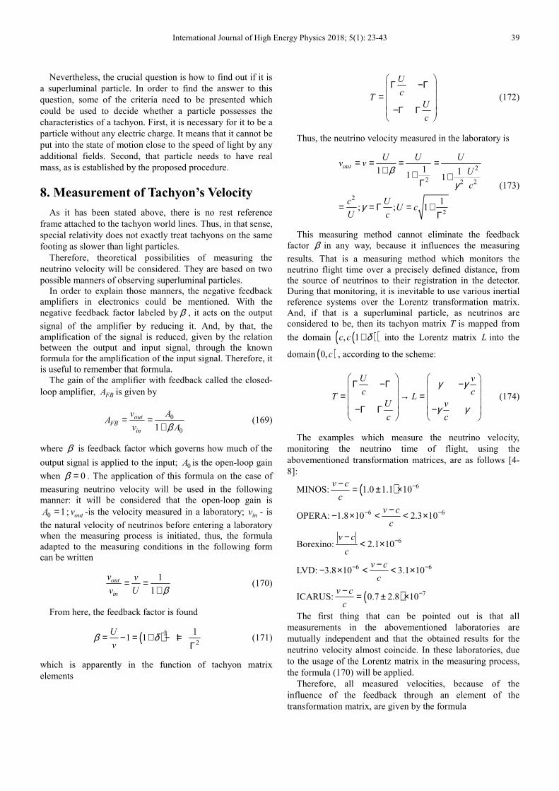
Nevertheless, the crucial question is how to find out if it is

a superluminal particle. In order to find the answer to this

question, some of the criteria need to be presented which

could be used to decide whether a particle possesses the

characteristics of a tachyon. First, it is necessary for it to be a

particle without any electric charge. It means that it cannot be

put into the state of motion close to the speed of light by any

additional fields. Second, that particle needs to have real

mass, as is established by the proposed procedure.

8. Measurement of Tachyon’s Velocity

As it has been stated above, there is no rest reference

frame attached to the tachyon world lines. Thus, in that sense,

special relativity does not exactly treat tachyons on the same

footing as slower than light particles.

Therefore, theoretical possibilities of measuring the

neutrino velocity will be considered. They are based on two

possible manners of observing superluminal particles.

In order to explain those manners, the negative feedback

amplifiers in electronics could be mentioned. With the

negative feedback factor labeled by β , it acts on the output

signal of the amplifier by reducing it. And, by that, the

amplification of the signal is reduced, given by the relation

between the output and input signal, through the known

formula for the amplification of the input signal. Therefore, it

is useful to remember that formula.

The gain of the amplifier with feedback called the closed-

loop amplifier, FBA is given by

0

01

outFB

in

v AA

v Aβ= =

+ (169)

where β is feedback factor which governs how much of the

output signal is applied to the input; 0A is the open-loop gain

when 0β = . The application of this formula on the case of

measuring neutrino velocity will be used in the following

manner: it will be considered that the open-loop gain is

0 1A = ; outv -is the velocity measured in a laboratory; inv - is

the natural velocity of neutrinos before entering a laboratory

when the measuring process is initiated, thus, the formula

adapted to the measuring conditions in the following form

can be written

1

1

out

in

v v

v U β= =

+ (170)

From here, the feedback factor is found

( )2

2

11 1 1

U

vβ δ= − = + − =

Γ (171)

which is apparently in the function of tachyon matrix

elements

U

cT

U

c

Γ −Γ = −Γ Γ

(172)

Thus, the neutrino velocity measured in the laboratory is

2

2 2 2

2

2

11 11 1

1; ; 1

out

U U Uv v

U

c

c UU c

U c

βγ

γ

= = = =+ + +Γ

= = Γ = +Γ

(173)

This measuring method cannot eliminate the feedback

factor β in any way, because it influences the measuring

results. That is a measuring method which monitors the

neutrino flight time over a precisely defined distance, from

the source of neutrinos to their registration in the detector.

During that monitoring, it is inevitable to use various inertial

reference systems over the Lorentz transformation matrix.

And, if that is a superluminal particle, as neutrinos are

considered to be, then its tachyon matrix T is mapped from

the domain ( )( ), 1c c δ+ into the Lorentz matrix L into the

domain ( )0,c , according to the scheme:

U v

c cT L

U v

c c

γ γ

γ γ

Γ −Γ − = → = −Γ Γ −

(174)

The examples which measure the neutrino velocity,

monitoring the neutrino time of flight, using the

abovementioned transformation matrices, are as follows [4-

8]:

MINOS: ( ) 61.0 1.1 10v c

c

−− = ± ×

OPERA: 6 61.8 10 2.3 10v c

c

− −−− × < < ×

Borexino: 62.1 10v c

c

−−< ×

LVD: 6 63.8 10 3.1 10v c

c

− −−− × < < ×

ICARUS: ( ) 70.7 2.8 10v c

c

−− = ± ×

The first thing that can be pointed out is that all

measurements in the abovementioned laboratories are

mutually independent and that the obtained results for the

neutrino velocity almost coincide. In these laboratories, due

to the usage of the Lorentz matrix in the measuring process,

the formula (170) will be applied.

Therefore, all measured velocities, because of the

influence of the feedback through an element of the

transformation matrix, are given by the formula



2

2

2 2

111 1 1

U U U cv

UU

c

β= = = =

+ + + −Γ

(175)

On the other hand, all results of laboratory measurements

are expressed in a relative relation with the speed of light

through the formula:

v c

cδ− = − (176)

From here, one gets

( )1 ; 11

cv c cδ δ

δ= − = < <<

+ (177)

And, of course, the measured velocity of neutrinos is

found by the formula:

2

1

c cv c

U δ= = <

+ (178)

that has been stated by all laboratories. Owing to the result

(178) obtained by this method, it is clearly seen that it is

impossible to measure the speed of superluminal particles,

even if they by any chance got in touch with a laboratory.

The reason for the occurrence of this result is in the influence

of the feedback factor β that is realized through the elements

of the tachyon matrix Γ and because of that influence, all

laboratories measure the velocity of neutrinos as below the

speed of light.

8.1. The Analysis of the Results of Emitted Neutrinos and

Photons of Light During the Explosion SN1987A

The second method of measuring neutrino velocity was

applied in the detection of neutrinos and photons of light

emitted during the explosion of Supernova SN1987A

168,000 light years away [14, 15]. In this case, the detectors

in laboratories registered the time moment of the reception of

the emitted neutrinos and photons of light. This measuring

method does not monitor the time of flight of the emitted

particles from the source to the detector over the inertial

reference systems that require mandatory usage of

transformation matrices. According to that, in this case, the

closed-loop gain equals one, because the feed-back factor

equals zero ( )0β = , and the formula (169) is reduced to the

form

1

1 0

outout in

in

v vv v U

v U= = → = =

+ (179)

This measuring method does not have the disrupting factor

in the form of a coefficient of tachyon or the Lorentz matrix

and, therefore, it should be expected that the measured

neutrino velocity is the right one.

During the explosion of Supernova SN1987A 168,000

years ago, neutrinos and photons of light reached the Earth

on 23rd

February 1987, when they were registered by the

detectors of laboratories. According to the reports of those

laboratories, published in the same year, neutrinos were

detected first and then, three hours later, the photons of light

were detected. The following explanation was provided for

the delay of the photons of light: Neutrinos arrived 3-4 hours

earlier than photons, because photons could not pass through

the outer layers of SN1987A before those layers got thin

enough. The analysis of those occurrences will be performed

and, then, on the basis of the obtained results, a suitable

comment will be provided. Thus, the conclusion in

contemporary physics is: Even though neutrinos arrived

earlier from the distance of 168,000 light years, where the

explosion SN1987A occurred, it has been concluded that they

are slower than light.

8.2. Case 1. The Assumption That Neutrinos Are Tachyons

and That They Are Simultaneously Emitted with

Photons

In this case, it is written:

( )( )

;1

1

L L L Lt t

U c c c

U c

δ

δ

+ ∆ = → + ∆ =+

= + (180)

and from here, one finds:

1U t

Lδ ∆= << (181)

From here, the following value forδ is found:

2

11

1

c t c t c t

c tL L L

L

c t c t c t

L L L

δ ∆ ∆ ∆ = ≈ + ∆ −

∆ ∆ ∆ = + ≈

(182)

Comment.

Let the estimation for δ be performed with the following

parameters:

1. Neutrinos arrived earlier for the time

3 3 3600t h s∆ = = × 2. Neutrinos had travelled the distance of

3 3

8

168 10 168 10 365 24 86400

3 10

L ly

m

= × = × × × ×

× ×

The calculated deviation above the speed of light is

710

c t

Lδ −∆= ≈ (183)

That would be approximate to the value obtained by the

laboratories [4-8] measuring the velocity of neutrinos:


710

v c

cδ −−= ≈ (184)

Taking into consideration (183), one gets the velocity of

neutrinos as tachyons

( ) ( )71 1 1 10

c tU c c c

Lδ −∆ = + = + ≈ +

(185)

Thus, the measured delay t∆ (181) of photons in relation

to neutrinos can occur only if neutrinos are superluminal

particles.

8.3. Case 2. The Example When Neutrinos Could Be

Subluminal

Let it be assumed that photons and neutrinos are

simultaneously emitted during the explosion SN1987A, but

that photons are delayed and the reason of that delay is said

to be: Photons had to wait until the envelope got thin enough

to be passed through. They are detained for the time period

t∂ until they start moving freely. For that time, neutrinos will

travel the way v t∂ , and the distance L , where the detector,

before photons for the measured interval t∆

( )ph

LL v t v t t v v t

c− ∂ = − ∆ = − ∆ (186)

From here, the photon delay is found

2

L Lt t

v c

L L Lt t

c c c

t t

δ

− + ∆ = ∂

+ − + ∆ = ∂ →

∂ = ∆

(187)

From this result it follows that, in case neutrinos are

subluminal, photons will arrive after neutrinos for the

measured time of t∆ if they get delayed in the explosion

process, 168,000 light years away, within SN1987A in the

time period of 2 6t t h∂ = ∆ ≈ .

Comment. The Sun produces photons in its core which

need around 50 million years of retention inside it until they

reach the outer rim, when they get emitted in the outer space

as sunlight.

During the SN1987A explosion, it is said that photons are

delayed: Photons had to wait until the envelope got thin enough

to be passed through. That detaining of photons, until the

envelope got thin enough, according to the given calculation,

lasted just 2 6t t h∂ = ∆ ≈ which had a consequence that, after

the travelled distance of 168000L ly≈ (ly=light year), they got

detected later for 3t h∆ ≈ at the detectors on the Earth in

comparison to neutrinos.

That long detention of photons during the SN1987A

explosion in relation to neutrinos should be the subject of

further research, because it is obviously one of the key

factors, as a physical phenomenon in defining the nature of

neutrinos.

9. Conclusions

In this theory, a tachyon has been considered as a particle

which possesses real mass but it is without rest mass.

It should be kept in mind that there is no rest reference

frame attached to the tachyon world lines. Therefore, in that

sense, special relativity does not really treat tachyons on the

same footing as slower than light particles.

Thus, for tachyons as superluminal particles there are no

rest frames because their velocities are restricted to below the

speed of light. However, the velocities are not restricted to

above it and, therefore, the limit of infinite velocities may

always be considered.

Based on the propositions of the physics of superluminal

particles, the following results obtained on the basis of this

theory can be underlined:

There are two points when tachyon energy has a tendency

towards the infinite value: the first point is at the speed of

light and the second one is at the infinite velocity. The

tachyon momentum at the speed of light has a tendency

towards the infinite value, but at the infinite velocity its value

is definite and equals mc .

As the main conclusion, it could be wondered:

1. Neutrinos as subluminal and independent particles, each

on their own, have the phase of final value. However, if

neutrinos can be independent, how can it be possible for

them to unite – combine and create the flavor state? And, by

that, to meet the condition for the flavor state oscillation? If

they possess the characteristic to combine – unite, then they

are no longer independent and autonomous. By uniting, they

lose their independence. However, what makes them unite, if

there is such a phenomenon? Do all of them unite or just

some of them? And, the ones that unite are no longer

autonomous. Thus, their autonomy and their uniting are two

features that are mutually exclusive. It is impossible to be

autonomous and, at the same time, to lose that autonomy by

joining other types of neutrinos. And, if they are just

autonomous, then, there is no mismatch between the flavor

state and mass states and, according to that, they will not

oscillate. Let it be shown how one may theoretically reach

the conclusion that neutrinos oscillate. As it has been shown,

neutrinos themselves are independent and each type has their

own phase. However, when the assumption of the mutual

time is introduced, they lose their independence. They mix

with each other creating the conditions for the occurrence of

the mismatch between mass states and flavor states.

Introducing that assumption provides the conditions for the

concurrence of the theory and experiment. Neutrinos, which

are in the first step autonomous each on their own, with the

introduction of the theoretical assumption of mutual time,

lose their autonomy. The question arises: to what extent is

that theoretical intervention correct, apart from the fact that

the obtained results match the experiment?

Now, let the focus shift to tachyons. First, by observing

tachyons independently of other particles, each type on its

own, they give the result that their phase equals zero. That

feature could be interpreted so that tachyons do not exist as



independent particles.

However, if tachyons existed, they would appear in nature

only and exclusively in a united state. Such a united and

combined state would provide the mismatch between flavor

states and mass states, which is in accordance with the

definition on flavor state oscillations.

In conclusion: Tachyons could not exist in nature as

independent particles. And, if they existed, they would

appear in a united state. Directly, all three types would mix

and combine according to the definition of the mismatch.

Such conclusion is derived on the basis of the theoretical

knowledge obtained. The first is that tachyons as independent

particles have zero phase and, therefore, could not exist in

nature. The second is that, opposite to tachyons, neutrinos as

subluminal particles could exist as independent particles.

However, that mutual independence of theirs opposes the

definition of the occurrence of oscillations. Owing to that, a

subsequent theoretical intervention has been introduced in

the neutrino physics; neutrinos lose their initial autonomy,

due to the need to concur with the experimental results.

However, theoretically observed, tachyons could lose their

independence by a simple introduction of mutual time or

their average velocity during movement into formulas for

phases, by which the conditions are met for their oscillating.

Thus, simply put, an autonomous – lone tachyon could not

exist in nature and, if it existed, it would appear united only

and exclusively together with other types of tachyons. To

emphasize once again:

1. Subluminal neutrinos could appear in nature as

independent particles

2. Such neutrinos, if they mixed with each other, would not

be independent from other types of neutrinos any more. This

contradicts the point 1.

3. From the points 1 and 2 it follows that subluminal

neutrinos could not mutually oscillate.

4. Subluminal neutrinos, theoretically observed, can be

made mutually dependent under a specific theoretical

condition, as is done in neutrino physics, in order to obtain

the concurrence of theoretical result with experiments.

For tachyons, we could also state the following:

1. In nature, there could not be a lone – autonomous or

isolated type of tachyons from other types.

2. If they existed in nature, then, a type of tachyons would

necessarily appear united with other types of tachyons.

3. The point 2 is in the direct accordance with the

definition on flavor state oscillations.

Therefore, observed theoretically, on the basis of overall

considerations, it could be concluded that the theoretical

result under the point 2 occurred not by introducing a

separate theoretical condition, but spontaneously. It is said

spontaneously because the appearance of one type of

tachyons in nature would be exclusively related to their

uniting with other types.

Comment. On the basis of theoretical considerations, it is

necessary to heed the following:

1. One type of tachyons could not exist in nature on its

own, lone and isolated from other types of tachyons.

2. One type of subluminal neutrinos could appear in nature

independent of other types of neutrinos.

3. A tachyon, if it existed in nature, would appear united

with other types of tachyons.

Thus, observing just points 2 and 3, it could be concluded:

On the basis of the point 2, the feature of subluminal

neutrinos would not be in accordance with the definition of

flavor state oscillations, whereas, on the basis of the point 3,

the feature of tachyons would be in accordance with that

definition.

It has been shown that it is impossible to measure the

velocities higher than the speed of light in certain

circumstances. A special attention has been devoted to the

method of measuring the velocity of neutrinos in

contemporary laboratories, as well as to the analysis of the

results of the arrival of neutrinos and photons in the

laboratories on the Earth, emitted during the explosion of

Supernova SN1987A.

References

[1] K. Nakamura et al (2010), “Review of particle physics”, Journal of Physics G Nucl. Part. Phys. 37075021.

[2] P. Hernandez, “Neutrino physics”, arxiv.1010.4131V1 [hep.-ph], 20 Oct. 2010 physics.

[3] Surender Verna, Theoretical and experimental status of neutrino physics: A brief review”. Hindawi Publishing Corporation, Volume 2015, Article ID 385968, 15 pages.

[4] Adamson, P. et.al., (2015), “Precision measurement of the speed of propagation of neutrinos using the Minos detectors”. Physical Review D. 92 (5):052005.

[5] OPERA Collaboration (2013), “Measurement of the neutrino speed with the OPERA detector in the CNGS beam using 2012 dedicated data”. Journal of High Energy Physics (1):153.

[6] ICARUS Collaboration (2012). “Precision measurement of the neutrino speed with the ICARUS detector in the CNGS beam”. Journal of High Energy Physics. 2012 (11):49.

[7] LVD Collaboration ), “Measurement of the velocity of neutrinos from the CNGS beam with the Large Volume Detector”. Physical Review Letters. 109 (7):070801.

[8] Borexino Collaboration (2012), “Measurement of CNGS muon neutrino speed with Borexino”. Physics Letters B. 716 (3-5):401-405.

[9] G. Feinberg, “Possibility of faster than light particles”, Physical Review 159 (5), 1089-1105, (1967).

[10] A. Chodos, “The neutrino as a tachyon”, Physics Letters B 150 (6) (1985), 431.

[11] Z. Todorovic, “Theory of tachyonic nature of neutrino”, Fund. Journal of Modern Physics, volume 6, Issues 1-2, 2013, pages 17-47.

[12] Z. Todorovic, “Neutrino oscillations founded on tachyon theory of neutrino”, International journal of astrophysics and space science, 2014; 2(6-1); 18-32.


[13] Z. Todorovic, “Interpretation of experimentally measured neutrino’s velocity based on neutrino’s tachyonic theory”, Fundamental journal of modern physics, Vol. 7, Issue 1, 2014, Pages 9-33. Published on line http:// www.frdint.com/.

[14] F. Vissani, et.al.,”What is the issue with 1987A neutrinos?”, arxiv:1008.4726v1[jep-ph], 27. Aug.2010.

[15] R. Valentim, et.al., “Evidence for two neutrino bursts from SN1987A ”, arxiv:1706.07824v1 [astro.-ph.hE], 2017.

[16] Ulrich D Jentschura, István Nándori and Robert Ehrlich” Calculation of the decay rate of tachyonic neutrinos against charged-lepton-pair and neutrino-pair Cerenkov radiation”, Journal of Physics G: Nuclear and Particle Physics, Volume 44, Number 10, 2017.

Documents

The Theoretic Research of Tachyons with Real Mass: …article.sciencepublishinggroup.com/pdf/10.11648.j.ijhep.20180501... · International Journal of High Energy ... The Theoretic