The Term Structure of Country Risk and

Valuation in Emerging Markets *

Juan José Cruces† Marcos Buscaglia†† Joaquín Alonso‡

First draft: Jan. 31, 02

This draft: May. 8, 02

Abstract

Most practitioners add the country risk to the discount rate in an ad-hoc manner when valuing projects

in Emerging Markets. This practice does not account for the fact that the default risk term structure

can be non-flat. The mismatch between the duration of the project being valued and the duration of

the most widely used measure of country risk, J.P. Morgan’s EMBI, leads to an overvaluation

(undervaluation) of long-term projects when the term structure of default risk is upward (downward)

sloping. Using sovereign bond data from five Emerging Markets, we estimate a simple model that

captures most of the variation of expected collection at different horizons for a given country at one

point in time. This model can be used to solve the misestimation problem.

JEL classification codes: G15, G31

Keywords : Emerging Economies, Cost of Capital, Default Risk

* We thank seminar participants at Univ. de San Andrés and Univ. Torcuato Di Tella for useful comments and

Gloria M. Kim from J.P. Morgan-Chase for kindly providing the panel of EMBI duration data. The most

current version of this paper will be posted at http://www.udesa.edu.ar/cruces/cc. Comments welcome.† Universidad de San Andrés, Argentina. E-mail address: cruces@udesa.edu.ar†† IAE School of Management and Business, Universidad Austral. Mariano Acosta s/n y Ruta Nac. 8, Casilla de

Correo 49, B1629WWA Pilar, Provincia de Buenos Aires, Argentina. Tel.: +54-2322-481069. E-mail

address: mbuscaglia@iae.edu.ar. Corresponding author.‡ Mercado Abierto, S.A., Buenos Aires, Argentina. E-mail address: joaquin@masa.com.ar.

1

I. Introduction

Investment projects in emerging markets are generally perceived as riskier than otherwise

similar projects in developed countries. The “additional risks” include currency

inconvertibility, civil unrest, institutional instability, expropriation, and widespread

corruption. Emerging markets (henceforth EM) are also more volatile than developed

economies: their business cycles are more intense, and inflation and currency risks are

higher.1

Several problems have restricted the use among practitioners of the Capital Asset Pricing

Model (CAPM) or its international version, the ICAPM, to calculate the cost of capital of

projects in EM. First, there is no complete agreement about the degree of integration of EM

capital markets to the world market (see Errunza and Losq, 1985, and Bekaert et al., 2001).

Second, local returns are non-normal, show significant first-order autocorrelation (Bekaert et

al., 1998), and there are problems of liquidity and infrequent trading (Harvey, 1995). Finally,

as correlations between local returns and international returns are so low, the cost of capital

that emerges from the use of these models appears as “too low”.

These problems have lead practitioners to account for the “additional risks” by making ad-

hoc adjustments to the CAPM. Godfrey and Espinosa (1996), for instance, propose to

calculate the cost of capital in EM (k) by using

( ) ( )fUS

mUS

US

ifUSi rrECSrkE −++=

σσ

6.0 (1)

where CS is the credit spread between the yield of a U.S. dollar-denominated EM sovereign

bond and the yield of a comparable U.S. bond, and the term preceding the last parenthesis is

1 Neumeyer and Perri (2001) find that output in Argentina, Brazil, Korea, Mexico and Philippines is at least

twice as volatile as it is in Canada.

2

an “adjusted beta”, that is equivalent to 60% of the ratio of the volatility of the domestic

market to that of the U.S. market.2

Although there are different versions of this model (see Pereiro and Galli, 2000, Abuaf and

Chu, 1994, and Harvey, 2000), all of them add the country risk to the U.S. risk free rate in

order to define the EM´s “analog” of the U.S. risk free rate.

There are few systematic surveys of cost of capital estimation practices in EM, but those

available show that variants of this model are the most widely used among practitioners.

Keck et al. (1998) find in a survey of Chicago School of Business graduates that in

international valuations most respondents adjust discount rates for factors such as political,

sovereign, or currency risks. Pereiro and Galli (2000) show that the vast majority of

Argentine corporations (including financial firms) add the country risk to the U.S. risk free

rate.3

Several objections have been raised in the literature to the addition of the country risk to the

discount rate. First, the model lacks any sound theoretical foundation (Harvey, 2000).

Second, in most versions of this model country risk is double counted, since part of the

variability in market returns is correlated with country risk (Estrada, 2000). The 60%

adjustment of Godfrey and Espinosa does not solve the problem, as it is completely ad-hoc.

Third, for global investors part of the country risk is diversifiable, and hence it should not be

included in the discount rate. Fourth, although this model gives a unique discount rate for all

projects, the “additional” risks inherent to EM do not have a uniform impact on all firms and

projects (Harvey, 2000). For example, the country risk may be high because the market

expects a sharp devaluation that would deteriorate the public sector’s financial position. A

devaluation, however, would benefit some sectors (e.g., exporters), and damage others (e.g.,

importers).

In this paper, we discuss another problem that the addition of country risk in the discount rate

as in equation (1) has; namely, that the mismatch between the duration of the project under

2 The 60% adjustment is due to the finding of Erb, Harvey and Viskanta (1995) that on average, about 40% of

the volatilities of emerging equity markets are explained by variations in credit quality. To avoid counting

twice the variation in credit spreads, only the fraction of equity variation that is unaccounted for by credit

spreads is taken into account --see Godfrey and Espinosa (1996) for details.

3

valuation and the duration of the most widely used measure of country risk leads to an

overvaluation (undervaluation) of long-term projects when the term structure of default risk is

upward (downward) sloping. The reverse is true for short-term projects.

The country risk measures most widely used are J.P. Morgan’s Emerging Market Bond Index

(EMBI), and its extensions EMBI+ and EMBI-Global (see for instance Pereiro, 2001). Using

these default risk measures in the discount rate to value long-term projects would bear no

additional problem to the ones mentioned above if the default risk term structure were flat.

But, in fact, this is not the case. In normal times, default risk spreads are low at the short end

of the curve and slope upward for longer durations. Often times, however, the default risk

term structure is downward sloping --as when the market expects a default in the short run

(see Figure I).

The mismatch between the duration of the project and the duration of the EMBI leads to an

overvaluation of long-term projects in the first case and to an undervaluation of them in the

second case. Figure I.C. illustrates this point: if, say, the project at hand had a duration of

four years and Argentina’s and Russia’s EMBI spreads had a duration of two years each,

valuation according to (1) would have overestimated the value of the Argentinean relative to

the Russian project.

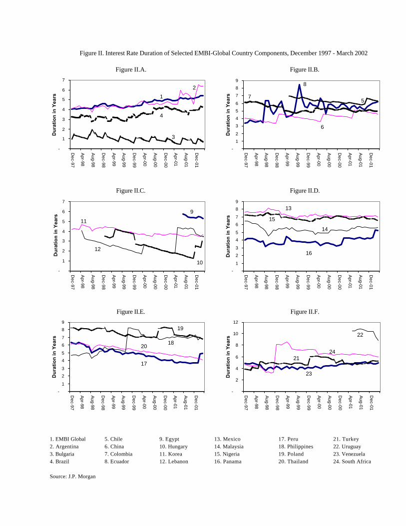
In addition, there is a high cross-country variability in the average duration of the EMBI-

Global country components (see Table I and Figure II). While the duration for Bulgaria is

lower than one year, for Hungary it is three years and for Uruguay it is higher than ten years

(Figure II). This variability undermines the significance of net present value comparisons of

otherwise similar projects in different countries, discounted in each country with the EMBI

Global as the country spread used in equation (1). For example, in June 2001 an investor

considering whether to locate a factory in Korea or in the Philippines would have used for

Korea a country spread corresponding to a duration of 3.6 years, whereas in the Philippines

he would have used a spread associated with a duration of 7.1 years.

Using sovereign bond data from five Emerging Markets, we estimate a simple model that

captures most of the variation in the sequence of expected collection for a given country at

one point in time. This model can be used to solve the misvaluation problem.

3 A number of important investment banks also add the country spread to the discount rate (Harvey, 2000).

4

The paper proceeds as follows. Section II explains the model used to estimate the default risk

term structure in EM sovereign debt markets and discusses the effects that a non-flat default

risk term structure has on the valuation of projects. Section III describes the data and section

IV presents the estimation results. Section V concludes.

II. The Model

II.1. Bond Prices and Expected Collection

Let r0,t be the yield to maturity implicit in prices of a risky sovereign zero-coupon bond

denominated in U.S. dollars issued at time 0 and maturing at time t. Similarly, let f0,t be the

expected return of holding this bond during the same time interval. We assume that EM

sovereign bonds carry no systematic risk and so f is the risk free rate. Let Qt be the

probability of full payment on this bond, and γ the recovery rate in the event of default. For a

one-period bond issued at time zero, these definitions imply

( ) ( ) ( ) 1,01,011,01 1111 frQrQ +=+−++ γ . (2)

Note that as long as there is some probability of default, tt fr ,0,0 > . Rearranging the left-hand

side gives the expected collection per dollar due, P1,

( )1,0

1,0111 1

11

r

fQQP

++

=−+= γ . (3)

Similarly, if there is another bond issued at t=0 and maturing at t=2, we have

( ) ( )22,0

22,02 11 frP +=+ . (4)

5

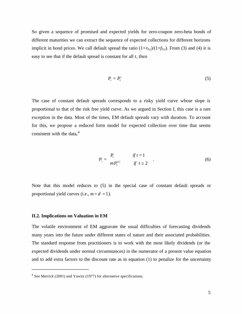
So given a sequence of promised and expected yields for zero-coupon zero-beta bonds of

different maturities we can extract the sequence of expected collections for different horizons

implicit in bond prices. We call default spread the ratio (1+r0,t)/(1+f0,t). From (3) and (4) it is

easy to see that if the default spread is constant for all t, then

tt PP 1= (5)

The case of constant default spreads corresponds to a risky yield curve whose slope is

proportional to that of the risk free yield curve. As we argued in Section I, this case is a rare

exception in the data. Most of the times, EM default spreads vary with duration. To account

for this, we propose a reduced form model for expected collection over time that seems

consistent with the data,4

≥

==

2

1

1

1

tifP

tifPP

tt δµ . (6)

Note that this model reduces to (5) in the special case of constant default spreads or

proportional yield curves (i.e., 1== δµ ).

II.2. Implications on Valuation in EM

The volatile environment of EM aggravate the usual difficulties of forecasting dividends

many years into the future under different states of nature and their associated probabilities.

The standard response from practitioners is to work with the most likely dividends (or the

expected dividends under normal circumstances) in the numerator of a present value equation

and to add extra factors to the discount rate as in equation (1) to penalize for the uncertainty

4 See Merrick (2001) and Yawitz (1977) for alternative specifications.

6

associated with the true expected dividends (see Keck et al., 1998, Pereiro and Galli, 2000,

Abuaf and Chu, 1994, Godfrey and Espinosa., 1996).

Consider the case of a firm located in an EM whose most likely outcome is that it will

produce a dividend of $d (constant) per period forever.5 Let MPr βτ +,0 be the constant per-

period discount rate stemming from (1), where τ stands for the interest rate duration of the

bond portfolio used to measure the country risk, and MPβ is analogous to the last term in

(1).6 In this case, the common practice is to compute the value of the firm as

MPrd

MPrd

Vt

t ββ ττ +=

++= ∑

∞

= ,01 ,0 )1(ˆ . (7)

We call V̂ “miscalculated value”, for reasons that become apparent below. Note that, from

(4),

ττ

ττ 1

,0,0

11

P

fr

+=+ , (8)

so that (7) is equivalent to

( )( ) τ

ττ

ττ

ττ

τττ

ττ

ββ11

,0

1

11

,0

1

11ˆ

PMPPf

dP

MPPf

dPV

tt

t

−++=

++= ∑

∞

=

(9)

5 We use “most likely dividends”, “central scenario dividends”, and “expected dividends under normal

circumstances” interchangeably.

6 Here τ,0r is the addition of the risk free rate plus the country spread in (1).

7

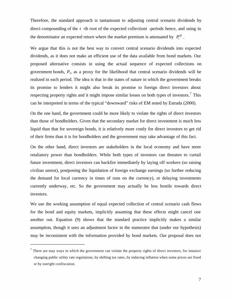
Therefore, the standard approach is tantamount to adjusting central scenario dividends by

direct compounding of the τ -th root of the expected collectionτ -periods hence, and using in

the denominator an expected return where the market premium is attenuated by ττ1P .

We argue that this is not the best way to convert central scenario dividends into expected

dividends, as it does not make an efficient use of the data available from bond markets. Our

proposed alternative consists in using the actual sequence of expected collections on

government bonds, Pt, as a proxy for the likelihood that central scenario dividends will be

realized in each period. The idea is that in the states of nature in which the government breaks

its promise to lenders it might also break its promise to foreign direct investors about

respecting property rights and it might impose similar losses on both types of investors.7 This

can be interpreted in terms of the typical “downward” risks of EM noted by Estrada (2000).

On the one hand, the government could be more likely to violate the rights of direct investors

than those of bondholders. Given that the secondary market for direct investment is much less

liquid than that for sovereign bonds, it is relatively more costly for direct investors to get rid

of their firms than it is for bondholders and the government may take advantage of this fact.

On the other hand, direct investors are stakeholders in the local economy and have more

retaliatory power than bondholders. While both types of investors can threaten to curtail

future investment, direct investors can backfire immediately by laying off workers (so raising

civilian unrest), postponing the liquidation of foreign exchange earnings (so further reducing

the demand for local currency in times of runs on the currency), or delaying investments

currently underway, etc. So the government may actually be less hostile towards direct

investors.

We use the working assumption of equal expected collection of central scenario cash flows

for the bond and equity markets, implicitly assuming that these effects might cancel one

another out. Equation (9) shows that the standard practice implicitly makes a similar

assumption, though it uses an adjustment factor in the numerator that (under our hypothesis)

may be inconsistent with the information provided by bond markets. Our proposal does not

7 There are may ways in which the government can violate the property rights of direct investors, for instance

changing public utility rate regulations, by shifting tax rates, by inducing inflation when some prices are fixed

or by outright confiscation.

8

provide a solution to the fact that expected collections may vary by sector of industry. Our

contribution is to compute the mispricing errors that arise from (9) when the term structure of

default risk is non flat and to provide a simple solution to adjust the valuation for any term

structure of expected collection. 8 Conditional on this assumption, the “true value”, V, of the

firm would be

∑∞

= +=

1 ,0 )1(tt

t

t

idP

V (10)

where i0,t is the expected rate of return of investing in this firm, and the numerator gives the

expected dividend each period. In equation (10) i0,t does not include the sovereign spread and

we can easily assume that it is constant (i.e., tii t ∀=,0 ). In financially integrated markets

where the CAPM holds, i would approximately be equal to the risk-free rate plus the beta of

the firm with respect to the world portfolio times the world market portfolio premium.9 In

segmented markets, beta and the market premium would be measured locally.10

If the default spread is constant, which we stress by using the subscript c, then (10) becomes,

( ) 1

1

1

1

11 PidP

i

dPV

tt

t

c −+=

+= ∑

∞

=

. (11)

Note that (11) gives approximately the same solution as (9), the only difference being in the

P that multiplies the market premium factor in (9).11

8 See Robichek and Myers (1966) and Chen (1967) for an old debate about the effects on discount rates of

alternative assumptions about the resolution of uncertainty over time.

9 Plus a term that reflects a premium for real exchange rate risk. See Adler and Dumas (1983).

10 Note that by explicitly using expected returns grounded on theory in the denominator, sector-specific

systematic risks can be accounted for in the discount rate.

11 Note from (5) that when the default spread is constant, ττ1

1 PP = .

9

Under the assumption that expected collections from bond markets apply to equities, the

practitioner approach would give the right valuation when the default spread is constant. But

bond markets seldom display such yield curve structures as shown in Figure I. In the more

general case in which µ and δ are not equal to one, plugging the expected collections from

(6) in (10) gives a value of the firm, Vv, as

−++

+= δ

δµ

1

21

1 11 PiP

Pi

dVv (12)

where the subscript v indicates that this holds for variable yield curve structures. Note that for

any value of µ and δ there is a value of r that makes vVV =ˆ , given by

−+

+

+=+

δ

δµβ

1

21

1

,0

1

1

Pi

PP

iMPr v (13)

We can interpret v as a time subscript referring to the duration of the risky bond (in a non-flat

yield curve context) whose yield used in the discount rate as in (7) would give a value of the

firm equivalent to that from (12). In Appendix I we show for 1== µτ that if ( )11 <> δδ ,

then )( ,0,0,0,0 ττ rrrr vv <> . Naturally, only when 1== δµ will vr ,0 be equal to τ,0r .

In general, the mismatch between the duration of the project and the duration of the bond

portfolio used to measure the discount rate as in equation (1) introduces a mispricing error

that we call m,

MPr

rr

VVV

m v

v

v

βτ

τ

+−

=−

=∧

,0

,0,0 (14)

10

The mispricing ratio has a straightforward interpretation. If the default spread is upward

sloping and τ is smaller than the duration of the project, v (so that τ,0,0 rr v > ), then the

standard practice overestimates the value of the project (m>0). This is because such method

uses in the numerator of (9) a direct compounding of an expected collection that is very high

for the short run , and that when compounded directly over time, gives values of expected

collections for long-run dividends that are too high relative to what is implicit in

contemporaneous long bond prices. Hence the overestimation.

Below, we use data from U.S. dollar-denominated EM bonds to estimate equation (6) and

illustrate the mispricing ratios that are likely to be observed for empirically reasonable values

of µ and δ .

III. Data

We collected effective annual ask yields and durations of non-guaranteed U.S. dollar-

denominated EM sovereign bonds (typically called “global bonds”). Data are from

Bloomberg for the last trading day of each month since September 1995 until December

2001. Also included are comparable U.S. Treasury yields, which are taken as the risk free

rate.

The sample was narrowed to those emerging countries which had data for more than one

bond at any point throughout the sample: Argentina, Brazil, Colombia, Ecuador, Mexico,

Poland, Russia, Thailand, Turkey, and Venezuela. Since we focus on yields spaced one-year

apart starting one year from the beginning of each period, we further narrowed the sample to

countries whose shorter traded bond had a duration smaller than 365 days for three months

that we considered representative of likely yield curve configurations: April 1997, January

2000 and August 2001. This restricted our sample to Argentina, Colombia, Mexico, Russia

and Turkey. 12 For those sample months for which the shortest bond had a duration greater

12 Appendix I lists the characteristics of all the included bonds. The only bond that is partially guaranteed is

Russia-99, which had debentures as collateral. If the bond were stripped, the non-guaranteed part of the bond

should have a greater duration and a higher yield, so the April 1997 Russian yield curve would have had an

even greater downward slope than that reported in Figure I.C.

11

than one year, we estimated the one-year yield by linear extrapolation of the two nearest

bonds available.

Figure I reports the yield curves for the sample considered, which were constructed by linear

interpolation of the available data.13 The horizontal axis shows the duration of the respective

bonds measured in years. None of the bonds considered are actually zero coupon. However,

we used the fact that for zero coupon bonds, duration and maturity are equal and that the

main determinant of yield for a given credit quality is duration. Therefore, we assumed that

each country had outstanding, at each month in the sample, a set of zero coupon bonds for

maturities at one year intervals into the future. The duration of the longest zero coupon bond

so constructed was smaller than that for the bond outstanding of highest duration. We

assumed that these bonds had no systematic risk and so set their expected returns equal to the

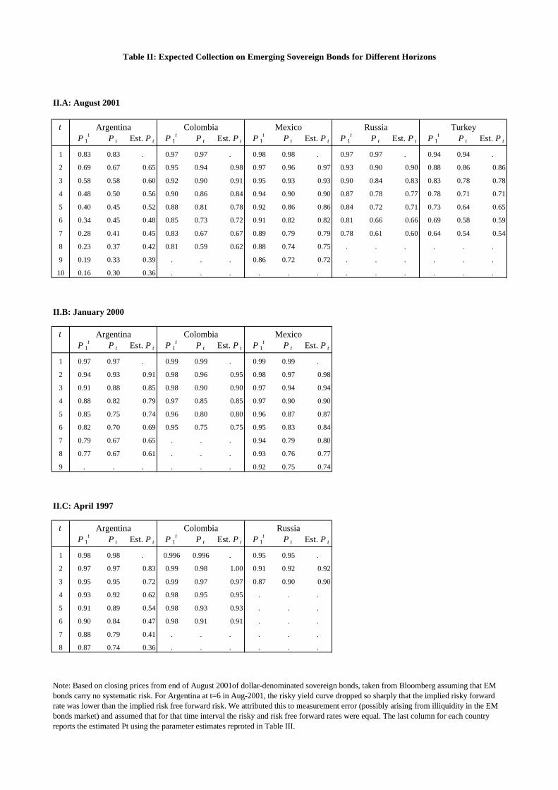
risk free rate for each duration. With this information we used equation (3) to estimate the

sequence of expected collections for different horizons that are consistent with EM sovereign

bond prices, which are shown in Table II.

It shows that while on some occasions tt PP 1≈ , it is often the case that they differ

substantially. For example, Figure I.A shows that Argentina had a negatively sloping yield

curve in August 2001. This translates in an expected collection for year 10 implicit in bond

prices of 0.30 (Table II.A), which is about twice the 0.16 that would result from direct

compounding of the first year expected collection. The converse is true for Colombia, which

had a steep yield curve at that time.

IV. Estimation Results and their Implications on Valuation in EM

IV.1. Estimation Results

With these data in hand, we estimated the empirical analog of equation (6),

( ) ( ) ( ) TtePtP tt ,...,2lnlnln 1 =++= δµ (15)

13 Plots of all available yields available are posted at http://www.udesa.edu.ar/cruces/cc/yield_curves.pdf.

12

separately for each country and for each month, by OLS. The rationale behind separate

estimation is that the yield curves in Figure I change dramatically across time and countries

so that assuming a model with constant parameters would be inadequate. This shortcoming

could be avoided by the use of conditioning information so that µ and δ depend on lagged

instruments. While that is an interesting approach that we propose to explore in future

research, it would lead us into yield curve modeling, an issue beyond the scope of this paper.

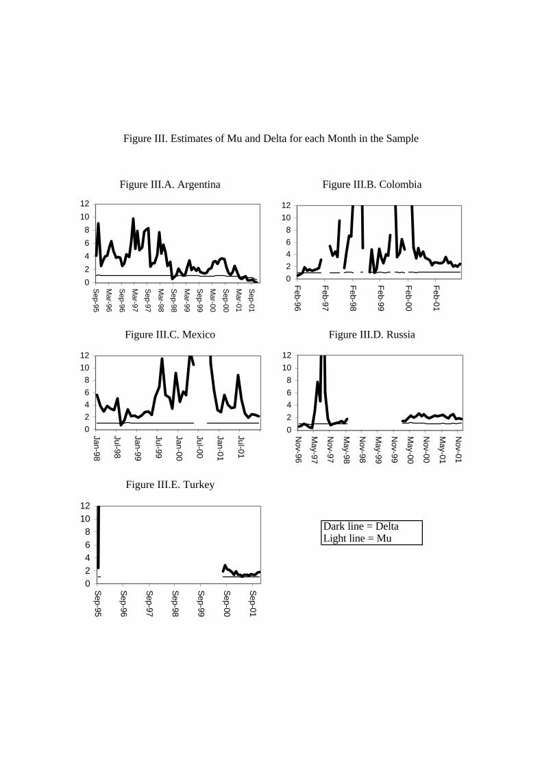
We estimated (15) for all months in the sample and report the key parameters. Figure III

reports the estimated µ and δ from (15) for all months in the sample. It is apparent that most

of the action of the expected collection model (6) is around the parameter δ , while µ is

rather stable around one over time for all countries. Most of the time δ is greater than one,

corresponding to an upward sloping default spread term-structure. Nevertheless, δ smaller

than one are not uncommon, as in Mexico and Argentina in mid-1998, Russia in early 1997,

Colombia around February 1996 and finally as Argentina approached the sovereign default of

2001.

Given the possible measurement error implicit in the extrapolation, we focus the subsequent

analysis on the results for three representative months at which the shortest traded bond had a

duration lower than one year.

Table III reports the results of estimating (15), and shows that the model fits well the

sequence of expected collection implicit in bond prices. It seems as though the variation of

expected collection for different horizons is well captured by a flexible power function of the

first period expected collection. All parameter signs agree with the intuition that when

sovereign spreads are upward sloping, sδ are greater than one, and conversely when they are

decreasing. It is noteworthy that all parameter estimates are statistically significantly different

from one --the maintained hypothesis in the standard practice reflected in equation (9) if the

τ used is one year. Sinceδ is the parameter that affects the expected collection as time passes,

it is the one that changes the most as the economic environment changes: from a minimum of

about 0.4 as countries approach default (Argentina in August 2001 and Russia in April 1997)

to about 8 when the yield curve steeps up.

13

IV.2. Implications for Valuation in Emerging Markets

This section reports the main findings of the paper. Table IV shows vr ,0 from (13), the

mispricing ratio m for 1=τ as in (14), and the duration of a constant free cash flow project,

for a range of parameter values that are consistent with the empirical estimates of µ , δ , P1,

and for values of the risk free rate that are consistent with real returns on long-term U.S.

government bonds. The mispricing ratios are computed assuming that β in (14) is zero

which is consistent with the evidence in Harvey (1995). 14

For µ =1 and δ =1.5, for instance (see top panel), the constant discount rate that would

correctly value the project is 12 percent, the estimated value using a constant discount rate of

9 percent (i.e., by assuming a flat term structure of default risk) would be 30 percent higher

than the true value.

The top and bottom panels differ only by the value of the risk-free rate (f). For a 95 percent

expected collection one year hence, the short-term risky rate is 9 percent when f is 4 percent

and it jumps to 12 when f equals 6.

When δ is less than one, the short-term sovereign spread is much higher than its long-term

counterpart and the estimated value can miss up to 35 percent of the true value. On the

contrary, when δ is larger than one, the estimated value under the current practice (using

1=τ ) can overestimate the true value of a project by a factor of about three or four.

For a given δ , �higher values of µ raise the true value relative to its estimated one since a

higher µ raises expected dividends. Naturally, when the yield curve steeps up, the constant

discount rate that would make the value of the project from (7) equal to that of (12) is much

higher than the short-term rate.

It should be noted that instead of calculating the first-year sovereign spread and assuming that

its term structure is flat, many practitioners use J.P. Morgan’s Emerging Bond Market Indices

(EMBI) as the measure of country risk in equation (1).

Table V uses actual sovereign yields for each duration to show the mispricing error that the

current practice may induce when the duration of the project differs from that of the bond

14 Note that if dividends grew over time, the durations of the projects would be even larger for a given r.

14

portfolio used to calculate the EMBI. In August 2001, for instance, the use of the EMBI

Global would have led to a 14 percent overvaluation of a project with a duration of seven

years in Colombia, and 3 percent in Russia. Errors range from overvaluations of up to 18

percent (Argentina in April 1997), to undervaluations of 6 percent (Mexico and Russia in

August 2001).

Note that these misestimation problems could be solved by using public information from

bond markets to estimate P1, µ and δ and, using equation (12) to appraise the correct value

of the project.

V. Conclusions and Further Research

Several problems have restricted practitioners from using the CAPM in order to estimate

discount rates in Emerging Markets, and have led them to account for the “additional” risks

of EM by adding the country risk to the discount rate.

In this paper we claim that such practice does not make an efficient use of the information

given by sovereign debt markets. In particular, it does not account for the fact that the default

risk term structure is non-flat and, hence, the mismatch between the duration of the project

under valuation and the duration of the most widely used measures of country risk, J.P.

Morgan’s EMBI, leads to an overvaluation (undervaluation) of long-term projects when the

term structure of default risk is upward (downward) sloping. The reverse is true for short-

term projects.

We establish that such practice amounts to reducing central scenario dividends by a power of

the expected collection for a horizon equal to the duration of the bonds used to measure the

country spreads. This would not be subject to additional criticisms to those already raised in

the literature if the default spreads were constant but it is problematic when they are not. In

normal times, however, default risk is low at the short end of the curve and slopes upward for

longer durations. Moreover, often times the default risk term structure is downward sloping --

as when the market expects a default in the short run.

15

In addition, there is a high cross-country variability in the average duration of the EMBI-

Global country components. This variability reduces the economic significance of net present

value comparisons of otherwise similar projects in different countries.

We use data from five EM to estimate a simple model of the term structure of default risk and

derive its implications on valuation. We find that by implicitly assuming that the term

structure of default risk is flat, mispricing errors in the range of minus 30 to plus 400 percent

can be made for reasonable parameter values. This mispricing can be avoided by using data

that are readily available from bond markets.

There are two directions for further research. First, it would be useful to generate expected

collections that vary by industrial sector, since the instability of EM has heterogeneous

impact across sectors (Eaton and Gersovitz, 1984). Second, by using conditioning

information to model the term structure of default risk, we could estimate how its shape

responds to fundamentals. If yield spreads are upward sloping in booms and downward

sloping in recessions, it would imply that the current valuation practice induces extra pro-

cyclicality in private investment in EM. This could be avoided by using our proposed

valuation approach.

Figure I. Yields on U.S. Dollar -Denominated Sovereign Bonds

Figure I.A. August 2001

05

10

15

20

2530

1 2 3 4 5 6 7 8 9Duration in Years

Yie

ld (%

poi

nts)

Argentina

USA

Mexico

ColombiaRussia

Turkey

Figure I.B. January 2000

4

6

8

10

12

14

1 2 3 4 5 6 7 8 9Duration in Years

Yie

ld (%

poi

nts)

Argentina

USA

Mexico

Colombia

Figure I.C. April 1997

4

6

8

10

12

1 2 3 4 5 6 7 8Duration in Years

Yie

ld (%

poi

nts) Argentina

USA

Colombia

Russia

1. EMBI Global 5. Chile 9. Egypt 13. Mexico 17. Peru 21. Turkey2. Argentina 6. China 10. Hungary 14. Malaysia 18. Philippines 22. Uruguay3. Bulgaria 7. Colombia 11. Korea 15. Nigeria 19. Poland 23. Venezuela4. Brazil 8. Ecuador 12. Lebanon 16. Panama 20. Thailand 24. South Africa

Source: J.P. Morgan

Figure II. Interest Rate Duration of Selected EMBI-Global Country Components, December 1997 - March 2002

Figure II.D.

Figure II.F.Figure II.E.

Figure II.C.

Figure II.A. Figure II.B.

-

1

2

3

4

5

6

7

Dec-97

Apr-98

Aug-98

Dec-98

Apr-99

Aug-99

Dec-99

Apr-00

Aug-00

Dec-00

Apr-01

Aug-01

Dec-01

Du

rati

on

in

Ye

ars 1

2

3

4

-

1

2

3

4

5

6

7

8

9

Dec-97

Apr-98

Aug-98

Dec-98

Apr-99

Aug-99

Dec-99

Apr-00

Aug-00

Dec-00

Apr-01

Aug-01

Dec-01

Du

rati

on

in

Ye

ars

5

6

7

8

-

1

2

3

4

5

6

7

Dec-97

Apr-98

Aug-98

Dec-98

Apr-99

Aug-99

Dec-99

Apr-00

Aug-00

Dec-00

Apr-01

Aug-01

Dec-01

Du

rati

on

in

Ye

ars

9

10

11

12

-

1

2

3

4

5

6

7

8

9

Dec-97

Apr-98

Aug-98

Dec-98

Apr-99

Aug-99

Dec-99

Apr-00

Aug-00

Dec-00

Apr-01

Aug-01

Dec-01

Du

rati

on

in

Ye

ars

13

14

15

16

-

1

2

3

4

5

6

7

8

9

Dec-97

Apr-98

Aug-98

Dec-98

Apr-99

Aug-99

Dec-99

Apr-00

Aug-00

Dec-00

Apr-01

Aug-01

Dec-01

Du

rati

on

in

Ye

ars

17

18

19

20

-

2

4

6

8

10

12

Dec-97

Apr-98

Aug-98

Dec-98

Apr-99

Aug-99

Dec-99

Apr-00

Aug-00

Dec-00

Apr-01

Aug-01

Dec-01

Du

rati

on

in

Ye

ars

21

22

23

24

Dark line = DeltaLight line = Mu

Figure III.E. Turkey

Figure III.A. Argentina Figure III.B. Colombia

Figure III. Estimates of Mu and Delta for each Month in the Sample

Figure III.C. Mexico Figure III.D. Russia

0

2

4

6

8

10

12

Sep-95

Mar-96

Sep-96

Mar-97

Sep-97

Mar-98

Sep-98

Mar-99

Sep-99

Mar-00

Sep-00

Mar-01

Sep-01

02468

1012

Feb-96

Feb-97

Feb-98

Feb-99

Feb-00

Feb-01

02468

1012

Jan-98

Jul-98

Jan-99

Jul-99

Jan-00

Jul-00

Jan-01

Jul-01

02468

1012

Nov-96

May-97

Nov-97

May-98

Nov-98

May-99

Nov-99

May-00

Nov-00

May-01

Nov-01

02468

1012

Sep-95

Sep-96

Sep-97

Sep-98

Sep-99

Sep-00

Sep-01

Dec-97 Jun-98 Dic 98 Jun-99 Dec-99 Jun-00 Dec-00 Jun-01 Dec-01EMBI Global 4.1 4.2 4.6 4.3 4.3 4.8 5.0 5.2 5.2Argentina 4.1 4.1 4.4 4.2 4.4 4.5 4.7 6.0 5.7Bulgaria 1.0 1.0 1.1 0.8 0.6 0.7 0.8 0.4 0.5Brazil 3.3 3.4 3.3 3.2 3.4 3.6 4.3 3.9 4.0Cote d"Ivoire 8.4 7.7 7.5 6.3 5.6 4.5 4.9 4.5Chile 6.9 6.6 6.3 6.1 6.0 6.5China 4.1 3.7 3.4 4.4 4.0 4.6 4.3 5.1 4.8Colombia 6.2 6.0 5.6 4.9 5.0 5.3 5.2 4.9 5.2Ecuador 3.4 3.8 5.0 4.5 5.4 6.1 5.5 5.7 5.9Greece 1.7 5.6 6.7 6.3 6.0Korea 4.2 4.5 4.3 4.2 3.8 3.6 3.6 3.6 3.6Lebanon 3.2 2.8 2.4 2.0 2.5 2.0 4.3 3.7Mexico 7.7 7.7 7.8 7.0 7.0 7.2 7.2 7.0 7.1Malaysia 6.5 5.7 5.2 5.6 5.3 4.9 5.3 5.5 5.6Nigeria 7.3 7.3 7.4 6.9 6.6 7.0 7.1 6.7 6.7Panama 4.0 3.8 3.5 3.9 3.7 3.5 3.3 4.1 4.2Peru 6.3 5.8 5.5 5.1 5.0 4.6 4.1 3.8 3.7Philippines 4.7 5.0 5.2 5.5 8.1 7.0 6.8 7.1 7.3Pakistan 2.2 2.0Poland 8.2 8.1 8.1 7.6 7.2 7.1 8.3 7.3 7.1Russia 5.3 5.4 5.8 6.2Thailand 6.2 6.0 5.9 5.7 5.4 5.1 4.9 4.6 4.3Turkey 3.9 5.2 4.8 4.6 4.6 6.0 5.2 4.9 5.2Ukraine 2.6 2.3 2.3 2.2Uruguay 10.5 10.4Venezuela 4.9 4.6 4.3 4.3 4.2 4.3 4.7 4.9 5.0South Africa 4.7 4.2 8.1 7.3 7.3 6.5 6.4 6.5 6.3

Source: J.P. Morgan

Table I: Interest Rate Duration of EMBI Global Country Components

tP 1

t P t Est. P t P 1t P t Est. P t P 1

t P t Est. P t P 1t P t Est. P t P 1

t P t Est. P t

1 0.83 0.83 . 0.97 0.97 . 0.98 0.98 . 0.97 0.97 . 0.94 0.94 .

2 0.69 0.67 0.65 0.95 0.94 0.98 0.97 0.96 0.97 0.93 0.90 0.90 0.88 0.86 0.86

3 0.58 0.58 0.60 0.92 0.90 0.91 0.95 0.93 0.93 0.90 0.84 0.83 0.83 0.78 0.78

4 0.48 0.50 0.56 0.90 0.86 0.84 0.94 0.90 0.90 0.87 0.78 0.77 0.78 0.71 0.71

5 0.40 0.45 0.52 0.88 0.81 0.78 0.92 0.86 0.86 0.84 0.72 0.71 0.73 0.64 0.65

6 0.34 0.45 0.48 0.85 0.73 0.72 0.91 0.82 0.82 0.81 0.66 0.66 0.69 0.58 0.59

7 0.28 0.41 0.45 0.83 0.67 0.67 0.89 0.79 0.79 0.78 0.61 0.60 0.64 0.54 0.54

8 0.23 0.37 0.42 0.81 0.59 0.62 0.88 0.74 0.75 . . . . . .

9 0.19 0.33 0.39 . . . 0.86 0.72 0.72 . . . . . .

10 0.16 0.30 0.36 . . . . . . . . . . . .

tP 1

t P t Est. P t P 1t P t Est. P t P 1

t P t Est. P t

1 0.97 0.97 . 0.99 0.99 . 0.99 0.99 .

2 0.94 0.93 0.91 0.98 0.96 0.95 0.98 0.97 0.98

3 0.91 0.88 0.85 0.98 0.90 0.90 0.97 0.94 0.94

4 0.88 0.82 0.79 0.97 0.85 0.85 0.97 0.90 0.90

5 0.85 0.75 0.74 0.96 0.80 0.80 0.96 0.87 0.87

6 0.82 0.70 0.69 0.95 0.75 0.75 0.95 0.83 0.84

7 0.79 0.67 0.65 . . . 0.94 0.79 0.80

8 0.77 0.67 0.61 . . . 0.93 0.76 0.77

9 . . . . . . 0.92 0.75 0.74

tP 1

t P t Est. P t P 1t P t Est. P t P 1

t P t Est. P t

1 0.98 0.98 . 0.996 0.996 . 0.95 0.95 .

2 0.97 0.97 0.83 0.99 0.98 1.00 0.91 0.92 0.92

3 0.95 0.95 0.72 0.99 0.97 0.97 0.87 0.90 0.90

4 0.93 0.92 0.62 0.98 0.95 0.95 . . .

5 0.91 0.89 0.54 0.98 0.93 0.93 . . .

6 0.90 0.84 0.47 0.98 0.91 0.91 . . .

7 0.88 0.79 0.41 . . . . . .

8 0.87 0.74 0.36 . . . . . .

Note: Based on closing prices from end of August 2001of dollar-denominated sovereign bonds, taken from Bloomberg assuming that EM bonds carry no systematic risk. For Argentina at t=6 in Aug-2001, the risky yield curve dropped so sharply that the implied risky forward rate was lower than the implied risk free forward risk. We attributed this to measurement error (possibly arising from illiquidity in the EM bonds market) and assumed that for that time interval the risky and risk free forward rates were equal. The last column for each country reports the estimated Pt using the parameter estimates reproted in Table III.

II.A: August 2001

II.B: January 2000

Argentina Colombia Mexico

II.C: April 1997

Argentina Colombia Russia

Table II: Expected Collection on Emerging Sovereign Bonds for Different Horizons

Russia TurkeyArgentina Colombia Mexico

T -1 µ δ R 2

Argentina 10 0.75 0.40 0.98(0.022) (0.019)

Colombia 7 1.14 2.86 0.96(0.04) (0.249)

Mexico 8 1.06 2.55 0.99(0.007) (0.07)

Russia 6 1.06 2.31 0.99(0.005) (0.029)

Turkey 6 1.04 1.50 0.99(0.007) (0.024)

T -1 µ δ R 2

Argentina 7 1.04 2.03 0.97(0.028) (0.169)

Colombia 5 1.07 7.33 0.99(0.008) (0.256)

Mexico 8 1.06 4.53 0.99(0.008) (0.159)

T -1 µ δ R 2

Argentina 7 1.10 7.86 0.97(0.02) (0.628)

Colombia 5 1.04 5.45 0.98(0.007) (0.4)

Russia 2 0.95 0.37 .. .

Minimum 0.75 0.37Maximum 1.14 7.86

Table III: Estimates of Mu and Delta for Different Samples

Estimated by OLS. Std. Errors in parentheses. For mu, standard errors are estimated using the delta method and so are approximate. Since only two observations (T -1=2) of P t are available for Russia in April 1997, we solved analytically for the two unknowns. No statistics are involved in that particular case.

April 1997

January 2000

August 2001

( ) ( ) ( ) TtePtP tt ,...,2lnlnln 1 =++= δµ

Assumptions: f = 4% P 1 = 0.95 r 1 = 9%µ Row

Content 0.5 0.8 1.0 1.5 2.5 4.0 7.00.8 r v |V=Vhat 8% 10% 12% 15% 22% 31% 50%

m -13% 8% 22% 58% 128% 232% 425%Dur. Proj. 13.1 10.7 9.6 7.7 5.6 4.2 3.0

1.0 r v |V=Vhat 7% 8% 9% 12% 18% 27% 44%m -29% -12% 0% 30% 90% 182% 362%

Dur. Proj. 15.9 13.0 11.6 9.1 6.6 4.7 3.31.1 r v |V=Vhat 6% 8% 9% 11% 17% 25% 41%

m -35% -19% -8% 19% 75% 162% 336%Dur. Proj. 17.3 14.1 12.5 9.9 7.0 5.0 3.4

Assumptions: f = 6% P 1 = 0.95 r 1 = 12%µ Row

Content 0.5 0.8 1.0 1.5 2.5 4.0 7.00.8 r v |V=Vhat 11% 13% 14% 17% 24% 34% 52%

m -7% 10% 22% 51% 109% 194% 351%Dur. Proj. 10.3 8.8 8.1 6.7 5.1 3.9 2.9

1.0 r v |V=Vhat 9% 10% 12% 14% 20% 29% 46%m -24% -10% 0% 25% 75% 151% 298%

Dur. Proj. 12.4 10.6 9.6 7.9 5.9 4.4 3.21.1 r v |V=Vhat 8% 10% 11% 13% 19% 27% 44%

m -31% -17% -8% 15% 61% 133% 276%Dur. Proj. 13.5 11.4 10.4 8.5 6.3 4.7 3.3

δ

δ

Table IV: Percentage Misestimation for Different Parameter Specifications

τ

τ

,0

,0,0

r

rr

VVV

m v

v

v−

=−

=∧

Spread over Treasury

Interest Rate

Duration1 2 3 4 5 6 7 8 9

August 2001

Argentina 14.3 5.7 4.3% 12.7% 15.0% 17.8% 15.4% -0.2% -0.8% -1.7% -2.7%

Colombia 4.4 5.1 -2.7% -3.7% -3.6% -2.4% -0.8% 6.8% 14.6% . .

Mexico 3.7 7.2 -3.1% -4.8% -5.1% -4.6% -2.8% -1.1% 1.2% 4.0% 5.2%

Russia 7.4 5.8 -4.6% -5.0% -4.6% -3.6% -2.3% -0.2% 2.9% . .

Turkey 9.7 4.8 -3.8% -4.4% -4.2% -2.7% -0.7% 0.3% 0.8% . .

January 2000

Argentina 5.7 4.4 -2.2% -3.1% -2.8% 0.0% 3.1% 4.5% 4.5% -0.9% .

Colombia 5.0 4.9 -4.0% -4.7% -3.3% -2.2% 0.5% 1.8% . . .

Mexico 3.6 7.2 -2.7% -4.0% -3.9% -2.5% -1.7% -0.5% 0.4% 1.2% -0.2%

April 1997

Argentina 2.2 3.9 -0.8% -1.1% -1.4% 0.0% 2.3% 6.4% 11.8% 18.5% .

Table V. Mispricing Error Using EMBI

EMBI Duration of the Investment Project in YearsPeriodand

Country

Appendix I

Let 1== µτ for simplicity and assume that β in (7) and (14). We want to show that if

( )11 <> δδ , then ).( ττ rrrr vv <> Assume that 1>δ but .τrrv ≤ This would imply that

t

t

t

t

v

fP

fp

fP

fp

rr

∑∑∞

=

∞

=

+

++

≥

+

++

⇔

≥

2

11

2

11

1111

11

δ

τ

For every t, the term between parenthesis on the left hand side is bigger than the

corresponding term on the right hand side if and only if 11 PP ≥δ , which is a contradiction.

Coupon Maturity Code ISIN Coupon Maturity Code ISIN

8.25% 15-Oct-97 (Arg-97) XS0040079641 7.125% 11-May-98 (Col-98) USP28714AE62

10.95% 1-Nov-99 (Arg-99) US040114AJ99 8% 14-Jun-01 (Col-01) US19532NAA46

9.25% 23-Feb-01 (Arg-01) US040114AK62 7.5% 1-Mar-02 (Col-02) US19532NAE67

8.375% 20-Dec-03 (Arg-03) US040114AH34 7.25% 15-Feb-03 (Col-03) US195325AH80

11% 4-Dec-05 (Arg-05) US040114BA71 10.875% 9-Mar-04 (Col-04) US195325AP07

11% 9-Oct-06 (Arg-06) US040114AN02 7.625% 15-Feb-07 (Col-07) US195325AK10

11.75% 7-Apr-09 (Arg-09) US040114BE93 8.625% 1-Apr-08 (Col-08) US195325AM75

11.375% 15-Mar-10 (Arg-10) US040114FC91 9.75% 23-Apr-09 (Col-09) US195325AR62

11.75% 15-Jun-15 (Arg-15) US040114GA27 11.75% 25-Feb-20 (Col-20) US195325AU91

11.375% 30-Jan-17 (Arg-17) US040114AR16

12.125% 25-Feb-19 (Arg-19) US040114BC38

12% 1-Feb-20 (Arg-20) US040114FB19 Coupon Maturity Code ISIN

9.75% 19-Sep-27 (Arg-27) US040114AV28 9.75% 6-Feb-01 (Mex-01) US593048AV35

10.25% 21-Jul-30 (Arg-30) US040114GB00 8.5% 15-Sep-02 (Mex-02) US593048AQ40

12.25% 19-Jun-18 (Arg-18) US040114GG96 9.75% 6-Apr-05 (Mex-05) US91086QAB41

12% 19-Jun-31 (Arg-31) US040114GH79 9.875% 15-Jan-07 (Mex-07) US593048BB61

0% 15-Mar-02 (LETE 90) ARARGE033134 8.625% 12-Mar-08 (Mex-08) US593048BF75

10.375% 17-Feb-09 (Mex-09) US593048BG58

9.875% 1-Feb-10 (Mex-10) US91086QAD07

Coupon Maturity Code ISIN 11.375% 15-Sep-16 (Mex-16) US593048BA88

8.75% 5-Oct-98 (Tur-98) XS0060514642 11.5% 15-May-26 (Mex-26) US593048AX90

9.00% 15-Jun-99 (Tur-99) US900123AC41

10% 23-May-02 (Tur-02) XS0076567774

8.875% 12-May-03 (Tur-03) XS0086996310 Coupon Maturity Code ISIN

11.875% 5-Nov-04 (Tur-04) US900123AK66 3% 14-May-99 (Rus-99) RU0004146067

9.875% 23-Feb-05 (Tur-05) XS0084714954 9.25% 27-Nov-01 (Rus-01) XS0071496623

10% 19-Sep-07 (Tur-07) XS0080403891 11.75% 10-Jun-03 (Rus-03) USX74344CZ79

12.375% 15-Jun-09 (Tur-09) US900123AJ93 8.75% 24-Jul-05 (Rus-05) XS0089372063

11.75% 15-Jun-10 (Tur-10) US900147AB51 8.25% 31-Mar-10 (Rus-10) XS0114295560

11.875% 15-Jan-30 (Tur-30) US900123AL40 11% 24-Jul-18 (Rus-18) XS0089375249

5% 31-Mar-30 (Rus-30) XS0114288789

* ISIN is the International Securities Identification Number.

Turkey

Russia

Appendix II: Characteristics of the Bonds Used

Argentina Colombia

Mexico

References

Abuaf, Niso, and Quyen Chu (1994), “The Executive´s Guide to International CapitalBudgeting: 1994 Update”, Salomon Brothers.

Adler, Michael and Bernard Dumas (1983), “International Portfolio Choice andCorporation Finance: A Synthesis,” Journal of Finance; 38(3), June , pp. 925-84.

Bekaert, Geert, Campbell Harvey, and Robin Lumsdaine (2001), “Dating theIntegration of World Equity Markets”, mimeo.

Bekaert, Geert, Claude Erb, Campbell Harvey and Tadas Viskanta (1998),“Distributional Characteristics of Emerging Markets Returns and Asset Allocation”,The Journal of Portfolio Management.

Chen, Houng-Yhi (1967), “Valuation under Uncertainty”, Journal of Financial andQuantitative Analysis, Volume 2, Issue 3, pp. 313-25.

Eaton, Jonathan and Mark Gersovitz (1984), “A Theory of Expropriation andDeviations From Perfect Capital Mobility, The Economic Journal, 94, March, pages16-40.

Erb, Claude, Campbell Harvey and Tadas Viskanta (1995), “Country Risk and GlobalEquity Selection,” Journal of Portfolio Management; 21(2), Winter, pp. 74-83.

Errunza, Vihang and Etienne Losq (1985), “International Asset Pricing under MildSegmentation: Theory and Test”, The Journal of Finance, Vol. XL, No. 1, pp. 105-24.

Estrada, Javier (2000), “The Cost of Equity in Emerging Markets: A Downside RiskApproach”, Emerging Markets Quarterly, 4 (Fall), pp. 19-30.

Godfrey, Stephen and Ramón Espinosa (1996), “A Practical Approach To CalculatingCosts of Equity for Investments in Emerging Markets”, Journal of AppliedCorporate Finance, Fall.

Harvey, Campbell (1995), “Predictable Risk and Returns in Emerging Markets”, TheReview of Financial Studies, Fall, Vol. 8, No. 3.

Harvey, Campbell (2000), “The International Cost of Capital and Risk Calculator(ICCRC)”, mimeo.

J.P. Morgan, “Emerging Markets Bond Index Monitor”, various issues.

Keck, Tom, Eric Levengood, and Al Longfield (1998), “Using Discounted Cash FlowAnalysis in an International Setting: A Survey of Issues in Modeling the Cost ofCapital”, Journal of Applied Corporate Finance, Fall.

Merrick, John J., Jr. (2001), “Crisis Dynamics of Implied Default Recovery Ratios:Evidence from Russia and Argentina,” Journal of Banking and Finance, October,v. 25, iss. 10, pp. 1921-39

Neumeyer, Pablo Andrés and Fabrizio Perri (2001), “Business Cycles in EmergingEconomies: The Role of Interest Rates”, mimeo.

Pereiro, Luis (2001), “The Valuation of Closely-Held Companies in Latin America,”Emerging Markets Review, 2, pp.330-70.

Pereiro, Luis and María Galli (2000), “La Determinación del Costo de Capital en laValuación de Empresas de Capital Cerrado: una Guía Práctica”, Working Paper(2000), Centro de Investigación en Finanzas, UTDT.

Robichek, Alexander and Stewart Myers (1966), “Conceptual Problems in the Use ofRisk-Adjusted Discount Rates”, The Journal of Finance, December, pp. 727-30.

Yawitz, Jess (1977), “An Analitical Model of Interest Rate Differentials and DifferentDefault Recoveries”, Journal of Financial and Quantitative Analysis, September,pp. 481-90.