Embed Size (px)
Citation preview
The Synergy of CFD and Experiments in Aerodynamics Researchat Cranfield University, Shrivenham
A. J. Saddington, K. Knowles and N. J. Lawson
Aeromechanical Systems Group,Department of Aerospace, Power and Sensors,
Cranfield University, RMCS, Shrivenham,Swindon, Wiltshire, SN6 8LA, UK
Keywords: LDV, PIV, CFD, supersonic, jet, transonic, cavity, racecar
Abstract
This paper discusses how the combined use of computational fluid dynamics and experimentation has been applied tothree particular fluid dynamics problems: high-speed turbulent jet flow, transonic cavity flows and open-wheeled race caraerodynamics. In each case knowledge gathered from one analysis technique has been used to assist in the applicationof the second technique thereby enabling greater understanding of the flow physics being studied than would have beenpossible through the isolated use of one or other methodology.
1 Introduction
For some time now, aerodynamics research carried out at Cranfield University’s Shrivenham Campus has made use ofboth experimental and numerical methods. The combination of these two disciplines has enabled greater understandingof the flow physics being studied than would have been possible through either a purely experimental or purelynumerical approach. Using examples of recent research projects, this paper will discuss the synergistic role that CFDand experiments have had in our aerodynamics research programme.
Early combined CFD and experimental research was primarily driven by the need for CFD validation e.g. [1]. Withcomputational resources limited, the experimental results were primarily used to validate the CFD models. The mainobjective was to give globally similar results to those measured in the experiments. The CFD was then used to reveallimited extra information on the flowfield.
More recently, improved computational resources have enabled refinements to the CFD models. Whilst CFD validationis still important, these models have provided additional insight into the physical processes involved, which were notdiscernable from the experimental measurements.
2 High-speed jet research
The rate at which a supersonic jet mixes with the surrounding ambient fluid is important for many aerospace applica-tions, notably in jet aircraft and rocket propulsion. For supersonic jets the generation of streamwise vortices appearsto be beneficial in improving mixing [2] and schemes have been investigated using vortex generators, tabs [3] and otherintrusive devices. This work [4,5] presents a numerical and experimental study of mixing in underexpanded, supersonicturbulent jets issuing from axisymmetric and castellated nozzles into quiescent conditions.
Experimental measurements using laser doppler velocimetry (LDV) and pitot probe measurements [6] along the jetcentreline at a nozzle pressure ratio (NPR = nozzle total to ambient static pressure ratio) of 4 indicated that the
1

castellated nozzles entrained more mass flow into the jet than a simple convergent nozzle. The CFD models verifiedthat this was the case but crucially also provided a physical explanation of the entrainment mechanism that wouldhave been very difficult to deduce from the available experimental data.
2.1 Nozzle design
Three castellated nozzles with convergent profiles and an exit diameter, D of 29.4 mm were investigated (Fig. 1). Eachnozzle had four regularly spaced castellations. The difference between the three nozzles was confined to the geometryof the gap between each castellation. The first nozzle (regular) had castellations cut by a radial line from the centre ofthe nozzle, as shown by the inner region of Fig. 2. The ‘outer region’ of Fig. 2 indicates alternative tooth designs (forall four teeth); radial position is as the ‘inner region’. The second nozzle (divergent chamfered) had castellations cutsuch that the gap between each nozzle was divergent in profile, as indicated by the ‘*’ on the outer region of Fig. 2.The third nozzle (convergent chamfered) had castellations cut such that the gap between each profile was convergentin profile, as indicated by the ‘**’ on the outer region of Fig. 2. The plain axisymmetric nozzle was of the same overallgeometry as the castellated ones but with the gaps between the teeth ‘filled in’ [7]. The mixing enhancement obtainedfrom the three castellated nozzle geometries was to be compared with the axisymmetric convergent nozzle [7].
Figure 1: Nozzle geometry showing the internal profile. Figure 2: Nozzle castellation configurations. Hatchedboxes indicate locations of teeth in nozzle lip: (*) al-ternative profile for divergent chamfered castellations;(**) alternative profile for convergent chamfered castel-lations.
2.2 Experiments
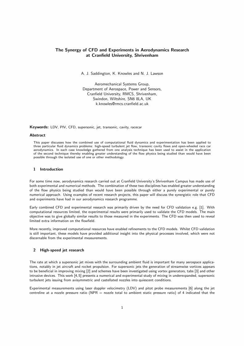
Experiments were conducted in a nozzle test cell at Shrivenham (Fig. 3). Data were collected for a NPR of 4. Three-dimensional LDV measurements were taken of the flow from the castellated nozzles. Seeding of the jet was by directinjection from a TSI six-jet seeder into the nozzle plenum chamber using JEM Hydrosonic seeding fluid.
Measurement traverses were made along the nozzle centreline, x. Probe access limited data collection to the first 10Dfrom the nozzle exit plane. The LDV measurements were estimated to be accurate to ±1% of velocity based on thesample time and frequency. Additional comparative data were taken from centreline LDV measurements of the plainaxisymmetric nozzle [4] and pitot probe measurements of the convergent chamfered castellated nozzle [6, 8] madepreviously under the same test conditions.
2
2.3 Numerical Model
The CFD model was developed using the Fluent commercial code (Version 5.5). The computational domain consistedof a three dimensional hexahedral mesh with approximately 250,000 to 450,000 cells depending on the test conditions.Only one quarter of the geometry was modelled since each nozzle has two axes of symmetry. The inlet plane wasapproximately 1D upstream of the nozzle exit, the outlet plane was at about 50D downstream and the radial boundarydiverged from 2D at the upstream end to more than 10D downstream.
Figure 3: LDV measurements in the nozzle test cell.
The boundary condition for the nozzle inlet was set as a pressure inlet with a prescribed total pressure, static pressure,total temperature and turbulence intensity. The turbulence intensity, Ti at nozzle inlet in the CFD model was adjustedto give the same nozzle exit turbulence intensity as the experiments (approximately 4%). The experimental Ti wasderived from the rms velocity data measured by the LDV technique. The turbulence length scale was set as 7.5%of nozzle radius [9]. The farfield boundary was set as a pressure outlet with a prescribed static pressure and statictemperature.
Turbulent calculations were performed using the RNG k-ε turbulence model [10], which has been shown to be suitablefor modelling under-expanded jets [11]. Initial axisymmetric calculations were conducted on a mesh of 14700 cells.Three stages of mesh adaption, based on density gradients greater than 1× 10⁻⁵ (to capture the shear layer) andMach numbers greater than 1.0 (to capture the shock core), were then performed. This reduced the grid spacing in theshock cell regions from 2 mm to 0.25 mm. Three stages of mesh adaption were sufficient to ensure a grid-independentsolution [7].
2.4 Mixing Enhancement
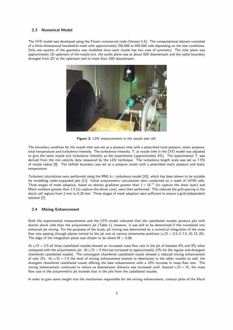
Both the experimental measurements and the CFD model indicated that the castellated nozzles produce jets withshorter shock cells than the axisymmetric jet (Table 1), however, it was still to be determined if this translated intoenhanced jet mixing. For the purposes of the study, jet mixing was determined by a numerical integration of the massflow rate passing through planes normal to the jet axis at various streamwise positions (x/D = 2.5, 5, 7.5, 10, 15, 20).The edge of the integration plane was chosen to be where M = 0.06.
At x/D = 2.5 all three castellated nozzles showed an increased mass flow rate in the jet of between 6% and 9% whencompared with the axisymmetric jet. At x/D = 5 this has increased to approximately 13% for the regular and divergentchamfered castellated nozzles. The convergent chamfered castellated nozzle showed a reduced mixing enhancementof only 2%. At x/D = 7.5 the level of mixing enhancement started to deteriorate in the other nozzles as well, thedivergent chamfered castellated nozzle offering the best enhancement with a 10% increase in mass flow rate. Themixing enhancement continued to reduce as downstream distance was increased until, beyond x/D = 15, the massflow rate in the axisymmetric jet exceeds that in the jets from the castellated nozzles.
In order to gain some insight into the mechanism responsible for the mixing enhancement, contour plots of the Mach
3
Axisymmetric Regular Convergent Divergent
x/D m(kgs−1
)m
(kgs−1
)% change m
(kgs−1
)% change m
(kgs−1
)% change
0.0 0.638 0.642 0.6 0.643 0.8 0.640 0.32.5 0.745 0.811 8.9 0.796 6.8 0.790 6.05.0 0.867 0.975 12.5 0.884 2.0 0.982 13.37.5 1.012 1.080 6.7 1.011 -0.1 1.110 9.7
10.0 1.172 1.192 1.7 1.166 -0.5 1.220 4.112.5 1.377 1.361 -1.2 1.325 -3.8 1.417 2.915.0 1.582 1.547 -2.2 1.557 -1.6 1.541 -2.617.5 1.795 1.770 -1.4 1.749 -2.6 1.794 -0.120.0 2.025 1.982 -2.1 1.961 -3.2 2.016 -0.425.0 2.476 2.458 -0.7 2.440 -1.5 2.483 0.330.0 2.953 2.916 -1.3 2.897 -1.9 2.937 -0.5
Table 1: CFD prediction of the mass flow rate of the four nozzles at various streamwise planes.
a).
z/D
y/D
-2 -1 0 1 2
-2
-1
0
1
2
Mach Number: 0.2 0.3 0.4 0.5 0.6 0.7 0.8 0.9 1 1.1 1.2 1.3 1.4 1.5 1.6 1.7 1.8 1.9 2 2.1 2.2 2.3
AxisymmetricDivergentChamfered
RegularConvergentChamfered
Gap
Nozzle lip
Tooth
b).
z/D
y/D
-2 -1 0 1 2
-2
-1
0
1
2
Mach Number: 0.2 0.3 0.4 0.5 0.6 0.7 0.8 0.9 1 1.1 1.2 1.3 1.4 1.5 1.6 1.7 1.8 1.9 2 2.1 2.2 2.3
AxisymmetricDivergentChamfered
RegularConvergentChamfered
c).
z/D
y/D
-2 -1 0 1 2
-2
-1
0
1
2
Mach Number: 0.2 0.3 0.4 0.5 0.6 0.7 0.8 0.9 1 1.1 1.2 1.3 1.4 1.5 1.6 1.7 1.8 1.9 2 2.1 2.2 2.3
AxisymmetricDivergentChamfered
RegularConvergentChamfered
d).
z/D
y/D
-2 -1 0 1 2
-2
-1
0
1
2
Mach Number: 0.2 0.3 0.4 0.5 0.6 0.7 0.8 0.9 1 1.1 1.2 1.3 1.4 1.5 1.6 1.7 1.8 1.9 2 2.1 2.2 2.3
AxisymmetricDivergentChamfered
RegularConvergentChamfered
Figure 4: CFD-predicted Mach number contours at various distances downstream of the nozzle exit: a). x/D = 2.5;b). x/D = 5; c). x/D = 7.5; d). x/D = 10.
4

number at each streamwise plane were examined for the CFD data (Fig. 4). At x/D = 2.5, the cross-sectional shapesof the jets are very different. The divergent chamfered nozzle produces a jet with a lobe of high velocity fluid, whichhas been ejected radially through the gap in the castellations. Similar fluid ejections, but of slightly different shapeswere observed for the other two castellated nozzle designs.
The CFD model showed that the increased jet mixing produced by the castellated nozzles appeared to be due todifferential expansion of the jet fluid in the gap and tooth regions as it leaves the nozzle exit. This differentialexpansion created a distorted jet cross section which presented a larger surface area to the ambient air, thus enablingmore rapid entrainment. The mixing enhancement was, however, confined to the nearfield flow (x/D < 10). At greaterstreamwise distances viscous dissipation appeared to cause the entrainment mechanism to decay resulting in mixingrates lower than an axisymmetric jet with final mass flow rates similar in each case. Although the mixing enhancementcould be determined experimentally, the entrainment mechanism responsible could only be determined from the CFD.
3 Transonic cavity flow
Transonic cavity flows over rectangular cavities are of particular relevance to aircraft weapons bays. For cavity lengthto depth ratios less than about 10 the flow is characterised by intense acoustic tones and flow unsteadiness. We presenthere numerical modelling and particle image velocimetry (PIV) measurements of a transonic cavity (M∞ = 0.85) witha length to depth ratio, L/D of 5 [12]. Here the numerical model is used to aid optimisation of the PIV set-up.
3.1 Numerical model
The CFD model was completed using commercial software GAMBIT + Fluent 6. The computational grid was createdfrom 86000 uniform quadrilateral cells with a distribution of 320× 65 cells within the cavity. The domain was designedto be geometrically similar to the wind tunnel test section. Thus, the upper and lower surface of the tunnel weremodelled with wall boundary conditions whilst the inlet and outlet conditions were modelled as the pressure far-fieldor free air condition. The flow problem was solved using the unsteady coupled solver and realisable k-ε turbulencemodel. The k-ε family of turbulence models was selected as a number of previous studies have shown it to performwell for flows with high shear and regions of recirculation.
3.2 Experimental Model
PIV data were taken from inside an all glass cavity of 160 mm length, 80 mm width and 32 mm depth. The cavityis made from 5 mm thick glass and is mounted in a modified tunnel wall. Due to the design of the transonic windtunnel test section it was not possible to image the entire cavity and into the freestream and the top 3 mm inside thecavity could not be mapped due to the presence of a metal flat plate. Details of the experimental set up are given inRitchie [12].
An in-house designed seeder injected a 5% glycerol and water solution into the contraction section of the wind tunnelfor the PIV measurements. The seeder consisted of an atomiser with 25 selectable jets and was supplied from themain tunnel air supply.
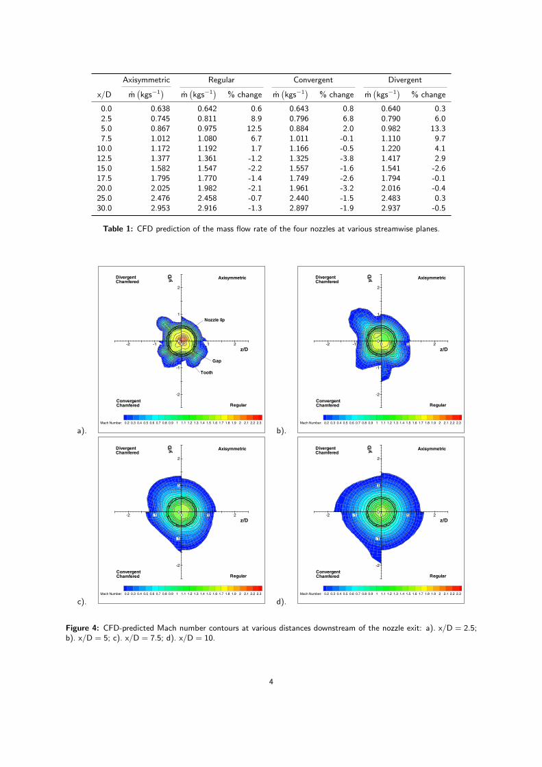
PIV images were recorded using a Kodak ES1.0 CCD with a 105 mm Micro-Nikor lens and a New Wave Geminidouble pulsed Nd:YAG laser. Sets of 70 images were taken for each run. Figure 5 shows a typical PIV image. Dataprocessing of the sets of 70 images was carried out using the TSI software UltraPIV with the Hart algorithm [13]. Theperformance of the UltraPIV algorithm, however, was found to be poor in regions of low seeding density. Therefore anin-house algorithm was also developed based on correlation averaging as proposed by Meinhart [14]. This was used toprocess the same 70 image set.
3.3 Experimental Optimisation
Lawson et. al. [15] have described an optimisation method for a double pulsed PIV experiment which can be appliedto autocorrelation or cross correlation analysis. They have shown that in order to retrieve a valid velocity vector froman interrogation region there exists a strong interdependence between the dynamic range, Dr of the flow defined by:
5
Figure 5: Typical instantaneous PIV particle image.
Dr =
∣∣∣∣Vmax
Vmin
∣∣∣∣ (1)
where Vmax and Vmin are the maximum and minimum velocities measured in the flow plane and the velocity gradientstrength, ϕ defined by:
ϕ =V2 − V1
Vmax(2)
Here, V2 − V1 is the velocity change across the interrogation region. A high dynamic range requirement necessarilyrestricts the strength of the velocity gradient in a chosen region and vice versa. The latter condition is crucial tothe design of a PIV experiment for use in transonic and supersonic flows. In any given experiment, other parameterscritical to the PIV system’s performance include the seeding density and corresponding particle image density, Ni
and the interrogation region size relative to particle image size, D/d. All these parameters must be considered whenoptimising the correlation performance whether using conventional correlation or the Hart correlation. In the lattercase, an equivalent number of particle images must be used by considering the surrounding interrogation regions.
With a-priori knowledge of Dr, ϕ and Vmax, D/d and Ni, it is possible to use the method to determine a laser pulseseparation, ∆t for a PIV experiment which will ensure that, on average, from a series of experiments at least 50% ofvalid vectors will be obtained from a ‘worst case’ interrogation region in the flow. The experiments are then definedas being optimised.
The CFD predictions provide the a-priori knowledge of Dr, ϕ, Vmax and Vmin, where the spatial resolution requirementwill determine the parameters D/d and Ni from the PIV experiment. The optimisation method will then yield arecommended magnification, M and pulse separation, ∆t.
The system magnification is defined in terms of the ratio of object and image distances and is that which is requiredto capture the flow area. The spatial resolution, L of the system is defined by:
L = D/M (3)
where D is the interrogation region length and the particle image size, d is dependent on the depth of field and laserpower of the system.
The CFD provided the a-priori information from inside the cavity listed in Table 2. The PIV requires a spacial resolutionof 1.5 mm. This leads to the experimental PIV values listed in Table 3.
Therefore if the particle image displacement is restricted to 20% of D and applying the optimisation method [15],yields a maximum allowable value of ϕDr = 1.5, which corresponds to ϕ = 21% given Dr = 7. Also, a magnificationof M = 1/16 must be used and a pulse separation ∆t = 30 ms. Since the maximum allowable value of ϕ = 21% isgreater than the CFD predicted value of ϕ = 15%, this means the PIV experiment will have sufficient performance toensure a minimum of 50% of valid vectors, on average, inside this region where the velocity gradients and dynamicrange are highest.
6

Parameter Value
Vmin
(ms−1
)-5
Vmax
(ms−1
)35
V2 − V1
(ms−1
)5
Dr 7ϕ (%) 15
Table 2: CFD a-priori values.
Parameter Value
L (mm) 1.5CCD size (pixels) 10002
Particle image size (pixels) 3D/d 10Ni 5
Table 3: Experimental parameter values.
3.4 Results
Figures 6 and 7 show time-averaged vector maps output from the PIV data processing from the Hart and the correlationaveraging algorithms. The results from the Hart algorithm do not show any substantial recirculation regions contraryto predictions by the CFD model. In contrast the results from the in-house correlation averaging algorithm show adistinct large scale recirculation inside the cavity. The poor performance of the Hart algorithm is attributed to locallylow levels of seeding inside the cavity as can be seen in the PIV image of Figure 5. Lower than expected seeding levelswould not provide the performance predicted by the optimisation method which assumed a minimum of 5 particleimages per interrogation region. The correlation averaging algorithm, however, ensures greater than 5 particles imagesper interrogation region as the 70 images set on average accumulates more than 5 particle images in each interrogationregion.
Figure 6: TSI code processed time averaged PIV vector map (70 Image average).
Figure 7: In House code processed time averaged PIV vector map (70 Image average).
The improved performance of the correlation averaging method is further illustrated in a U component centrelineplot of velocity shown in Figure 8. In this case the TSI data has a greater deviation than the correlation averagedresults when compared to the CFD prediction. Therefore optimisation of a given PIV system requires not just a-prioriknowledge of the flow to specify variables such as M and ∆t, but also careful control of variables such as seeding andjudicious choice of the data processing algorithms for a given flow.
4 Open-wheeled racecars
Ground simulation and wheel rotation are known to be essential for accurate automotive testing [16], particularly foropen-wheeled racecars. With this type of vehicle, ground effects and large unfaired wheels dominate their aerodynamiccharacteristics. Every care must be taken to ensure that the wheels are modelled correctly both in experimental testing
7

Figure 8: Streamwise Velocity Profile - y/d=0.5.
and computational simulation. Previous evaluations of the capability of CFD to model wheel flows [17–19] used thesurface pressure and force data published by Fackrell [20,21] as their main validation criteria.
CFD models enable researchers to investigate physical processes that may be impossible to reproduce experimentally.In our work the investigation concentrated on the effect of using external wheel support struts during racecar windtunnel testing [22]. The struts are used to mechanically decouple the car body from the ground whilst still allowing thewheels to rotate. Ideally the support struts should be aerodynamically neutral, however, this is not always the case.
An experimentally validated CFD model of an isolated racecar wheel and strut was used to quantify the aerodynamicinterference effects between the two. The virtual environment of the CFD model enabled the support strut to be easilyremoved, something that could not have been carried out experimentally.
4.1 Experiments
A 40% scale (263 mm diameter), non-deformable Champ Car front wheel assembly was chosen along with its associatedsupport sting. The experimentally tested sting was of aluminium beam section with a symmetrical aerofoil profile. Itsupported a 50 N load cell, oriented to measure drag force, to which the wheel was attached. The aerofoil profile wasextended to the wheel by shrouding the load cell with carbon fibre. The instrumentation cabling was shielded from thefreestream air by routing it inside the sting. No vertical force, other than that due to the weight of the components,was applied during testing and no problems were encountered with wheel lift. The experimental set-up is shown inFigure 9.
The LDV measurements were made using a two-component and a single-component, 1m focal length, Dantec FibreFlowprobes mounted to a three-component traverse. Data acquisition was carried out by three BSA enhanced signalprocessors, with all equipment centrally controlled by Dantec Burstware software.
The experimental set-up was tested at 20 ms−1, corresponding to a Reynolds number (based on wheel diameter)of 3.69× 10⁵. LDV measurements were made in four vertical planes oriented perpendicular to the freestream flow.Traverse access confined each plane to being a 250 mm square, centred about the longitudinal centreline of the wheel.The planes were located at 10, 25, 50 and 100 mm downstream of the rearmost part of the wheel and containedidentical grids of 441 equally-spaced data points. All three velocity components were simultaneously sampled over a15 second period yielding 2500 samples for each component at each point. When processed, these data subsequentlyprovided time-averaged three-dimensional velocity results.
8

4.2 Numerical model
The wheel and sting assembly was placed in a rectangular domain with the inlet 5 wheel diameters upstream, outlet16 wheel diameters downstream, a width of 10 and a height of 5 wheel diameters. The interior of the sting was alsomeshed to allow it to be removed from the solution domain by allowing fluid to flow through it, thus eliminating theneed to generate an entirely new mesh for that section of the study.
The only significant deviation from the experimental geometry was made at the tyre contact patch. Difficulty wasencountered in maintaining high cell quality when modelling the near line-contact between the rolling road and non-deformable tyre. Therefore, the wheel was slightly truncated by raising the ground plane by 0.8mm. This increasedthe size of the contact patch and greatly improved the cell skewness in this area. The final mesh was of the order of0.93 million cells. Figure 10 shows the surface mesh on the wheel and sting assembly.
Figure 9: Experimental Set-up Figure 10: CFD Surface Mesh of Wheel Assembly andSupport Sting
The boundary conditions of the CFD simulation were chosen to be representative of those of the experiment. Auniform flow with a velocity of 20 ms−1 was specified at the inlet and standard atmospheric pressure specified at theoutlet. The rolling road and wheel components were modelled as translating and rotating walls respectively, all witha linear velocity of 20 ms−1. When simulating the wheel and sting, the sting surface was specified as a wall with theno-slip condition applied. When testing the wheel without the sting, the latter’s surface was represented by an interiorcondition, which did not impede flow. The mesh inside the sting was solved as a fluid, effectively removing the stingfrom the domain. Symmetry planes represented the remaining domain boundaries. Simulations were run with the k-ωturbulence model.
4.3 Validation
The mean drag force calculated from the experimental data was non-dimensionalised by the frontal area of the wheel.The drag coefficient, CD predicted by the CFD simulation was 0.638, which was 6.2% lower than the measured valueof 0.680.
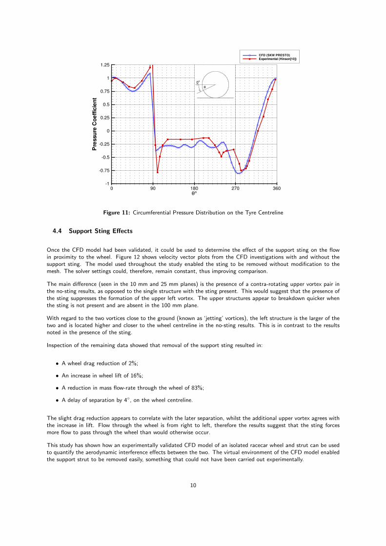
Care should be exercised when using force data as the sole accuracy measure [23] but the good experimental velocitycorrelation supported the validity of this prediction. This was further reinforced by inspection of the circumferentialstatic pressure coefficient, Cp on the centreline of the tyre surface, Figure 11. Although surface Cp was not measuredexperimentally, comparison can be made with the work of Hinson [24]. This presented the pressure coefficients onthe surface of a Formula One wheel, measured using transducers mounted within. Comparison was made with resultstaken from tests at the same Reynolds number as, and using a geometrically similar wheel to, this investigation. Theresults show good correlation and illustrate several important features. CFD predicted the separation 22◦ late at 244◦
as opposed to 266◦ measured by Hinson. Also, the base pressure was under-predicted just downstream of separation.Both factors would lead to an under-prediction of drag coefficient and are believed to be responsible, along withexperimental errors, for the discrepancy seen in this study.
9
θ°
Pre
ssur
eC
oeffi
cien
t
0 90 180 270 360-1
-0.75
-0.5
-0.25
0
0.25
0.5
0.75
1
1.25
CFD (SKW PRESTO)Experimental (Hinson[10])
0o
θ
Figure 11: Circumferential Pressure Distribution on the Tyre Centreline
4.4 Support Sting Effects
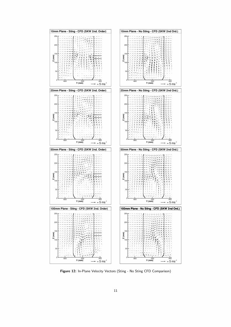
Once the CFD model had been validated, it could be used to determine the effect of the support sting on the flowin proximity to the wheel. Figure 12 shows velocity vector plots from the CFD investigations with and without thesupport sting. The model used throughout the study enabled the sting to be removed without modification to themesh. The solver settings could, therefore, remain constant, thus improving comparison.
The main difference (seen in the 10 mm and 25 mm planes) is the presence of a contra-rotating upper vortex pair inthe no-sting results, as opposed to the single structure with the sting present. This would suggest that the presence ofthe sting suppresses the formation of the upper left vortex. The upper structures appear to breakdown quicker whenthe sting is not present and are absent in the 100 mm plane.
With regard to the two vortices close to the ground (known as ‘jetting’ vortices), the left structure is the larger of thetwo and is located higher and closer to the wheel centreline in the no-sting results. This is in contrast to the resultsnoted in the presence of the sting.
Inspection of the remaining data showed that removal of the support sting resulted in:
• A wheel drag reduction of 2%;
• An increase in wheel lift of 16%;
• A reduction in mass flow-rate through the wheel of 83%;
• A delay of separation by 4◦, on the wheel centreline.
The slight drag reduction appears to correlate with the later separation, whilst the additional upper vortex agrees withthe increase in lift. Flow through the wheel is from right to left, therefore the results suggest that the sting forcesmore flow to pass through the wheel than would otherwise occur.
This study has shown how an experimentally validated CFD model of an isolated racecar wheel and strut can be usedto quantify the aerodynamic interference effects between the two. The virtual environment of the CFD model enabledthe support strut to be removed easily, something that could not have been carried out experimentally.
10
Y (mm)
Z(m
m)
-600 -500 -4000
50
100
150
200
250
= 5 ms-1
10mm Plane - Sting - CFD (SKW 2nd. Order)
Y (mm)
Z(m
m)
-600 -500 -4000
50
100
150
200
250
= 5 ms-1
25mm Plane - Sting - CFD (SKW 2nd. Order)
Y (mm)
Z(m
m)
-600 -500 -4000
50
100
150
200
250
= 5 ms-1
50mm Plane - Sting - CFD (SKW 2nd. Order)
Y (mm)
Z(m
m)
-600 -500 -4000
50
100
150
200
250
= 5 ms-1
100mm Plane - Sting - CFD (SKW 2nd. Order)
Y (mm)
Z(m
m)
-600 -500 -4000
50
100
150
200
250
= 5 ms-1
10mm Plane - No Sting - CFD (SKW 2nd Ord.)
Y (mm)
Z(m
m)
-600 -500 -4000
50
100
150
200
250
= 5 ms-1
25mm Plane - No Sting - CFD (SKW 2nd Ord.)
Y (mm)
Z(m
m)
-600 -500 -4000
50
100
150
200
250
= 5 ms-1
50mm Plane - No Sting - CFD (SKW 2nd Ord.)
Y (mm)
Z(m
m)
-600 -500 -4000
50
100
150
200
250
= 5 ms-1
100mm Plane - No Sting - CFD (SKW 2nd Ord.)100mm Plane - No Sting - CFD (SKW 2nd Ord.)
Figure 12: In-Plane Velocity Vectors (Sting - No Sting CFD Comparison)
11

5 Conclusions
In this paper we have illustrated how the combined use of computational fluid dynamics and experimentation hasbeen applied to three particular fluid dynamics problems: high-speed turbulent jet flow, transonic cavity flows andopen-wheeled race car aerodynamics. In each case knowledge gathered from one analysis technique has been usedto assist in the application of the second technique thereby enabling greater understanding of the flow physics beingstudied than would have been possible through the isolated use of one or other methodology. The authors would liketo acknowledge the work of Simon Ritchie and Robin Knowles in support of this paper.
References
[1] Knowles, K. and Bray, D., “Computation of Normal Impinging Jets in Cross-flow and Comparison with Experiment,”International Journal of Numerical Methods in Fluids, Vol. 13, No. 10, December 1991, pp. 1225–1233.
[2] Samimy, M., Reeder, M. F., and Zaman, K., “Supersonic Jet Mixing Enhancement by Vortex Generators,”AIAA/SAE/ASME/ASEE 27th Joint Propulsion Conference, Sacramento, CA, USA, 24-26 June 1991, No. 91-2263.
[3] Samimy, M., Zaman, K. B. M. Q., and Reeder, M. F., “Effect of Tabs on the Flow and Noise Field of an AxisymmetricJet,” AIAA Journal , Vol. 31, No. 4, April 1993, pp. 609–619.
[4] Saddington, A. J., Lawson, N. J., and Knowles, K., “Numerical Predictions and Experiments on Supersonic Jet Mixingfrom Castellated Nozzles,” 23rd Congress of the International Council of the Aeronautical Sciences, Toronto, Canada, 8-13September 2002.
[5] Saddington, A. J., Knowles, K., and Wong, R. Y. T., “Numerical Modelling of Mixing in Jets from Castellated Nozzles,”The Aeronautical Journal of the RAeS , Vol. 106, No. 1066, December 2002, pp. 643–652.
[6] Knowles, K. and Wong, R. Y. T., “Passive Control of Entrainment in Supersonic Jets,” RAeS Aerodynamics ResearchConference, London, 17-18 April 2000, pp. 9.1–9.14.
[7] Saddington, A. J., Lawson, N. J., and Knowles, K., “Simulation and Experiments on Under-expanded Turbulent Jets,”CEAS Aerospace Aerodynamics Research Conference, Cambridge, UK, 10-13 June 2002.
[8] Wong, R. Y. T., Enhancement of Supersonic Jet Mixing , Ph.D. thesis, Department of Aerospace, Power and Sensors,Cranfield University, July 2000.
[9] Rodi, W., Turbulence Models and their Application in Hydraulics - A State of the Art Review , International Association forHydraulic Research, Rotterdamseweg 185 - P.O. Box 177, 2600 MH Delft, The Netherlands, 2nd ed., 1984.
[10] Yakhot, A. and Orszag, S. A., “Renormalisation Group Analysis of Turbulence: I. Basic Theory,” Journal of ScientificComputing , Vol. 1, No. 1, 1986, pp. 1–51.
[11] Knowles, K. and Saddington, A. J., “Modelling and Experiments on Underexpanded Turbulent Jet Mixing,” 5th InternationalSymposium on Engineering Turbulence Modelling and Measurement, Mallorca, Spain, 16-18 September 2002.
[12] Ritchie, S. A., Lawson, N. J., and Knowles, K., “An Experimental and Numerical Investigation of an Open TransonicCavity,” 21st AIAA Applied Aerodynamics Conference, Orlando, Florida, USA, 23-26 June 2003, Paper No. 2003-4221.
[13] Hart, D. P., “PIV error correction,” Experiments in fluids, Vol. 29, No. 1, 2000, pp. 13–22.
[14] Meinhart, C., Wereley, S., and Santiago, J., “A PIV Algorithm for Estimating Time-Averaged Velocity Fields,” Journal ofFluids Engineering , Vol. 122, No. 2, June 2000, pp. 285–289.
[15] Lawson, N. J., Coupland, J. M., and Halliwell, N. A., “A Generalised Optimisation Method for Double Pulsed Particle ImageVelocimetry,” Optics and Lasers in Engineering , Vol. 27, No. 6, August 1997, pp. 637–656.
[16] Hackett, J. E., Baker, J. B., Williams, J. E., and Wallis, S. B., “On the influence of ground movement and wheel rotationin tests on modern car shapes,” Paper 870245, Society of Automotive Engineers, 1987.
[17] Skea, A. F., Bullen, P. R., and Qiao, J., “The Use of CFD to Predict the Air Flow Around a Rotating Wheel,” 2nd MIRAInt. Vehicle Aerodynamics Conf , UK, 1998.
[18] Basara, B., Beader, D., and Przulj, V. P., “Numerical Simulation of the Airflow around a Rotating Wheel,” 3rd MIRA Int.Vehicle Aerodynamics Conf , UK, 2000.
[19] Axon, L., Garry, K., and Howell, J., “An Evaluation of CFD for Modelling the Flow Around Stationary and Rotating IsolatedWheels,” Paper 980032, Society of Automotive Engineers, 1998.
[20] Fackrell, J. E., The Aerodynamic Characteristics of an Isolated Wheel Rotating in Contact with the Ground , Ph.D. thesis,Imperial College of Science and Technology, London, 1972.
[21] Fackrell, J. E. and Harvey, J. K., “The Flow Field and Pressure Distribution of an Isolated Road Wheel,” Advances in RoadVehicle Aerodynamics, Paper 10, BHRA, London, 1973, pp. 155–165.
[22] Knowles, R. D., Saddington, A. J., and Knowles, K., “Simulation and Experiments on an Isolated Road Wheel Rotating inGround Contact,” 4th MIRA International Vehicle Aerodynamics Conference, Warwick, UK, 16-17 October 2002.
[23] Makowski, F. T. and Kim, S.-E., “Advances in External-Aero Simulation of Ground Vehicles Using the Steady RANSEquations.” Vehicle Aerodynamics SP-1524 , Paper 2000-01-0484, Society of Automotive Engineers, 2000.
[24] Hinson, M., Measurement of the Lift Produced by an Isolated, Rotating Formula One Wheel Using a New Pressure Mea-surement System, MSc thesis, Cranfield University, 1999.
12