The Survey Response Process in Telephone and Face-to-Face Surveys:

Differences in Respondent Satisficing and Social Desirability Response Bias

Melanie C. Green

University of Pennsylvania

and

Jon A. Krosnick and Allyson L. Holbrook

The Ohio State University

April, 2001

The authors wish to express their thanks to Virgina Sapiro, Kathy Cirksena, James Lepkowski, Robert Belli, Robert Groves, Robert Kahn, John Van Hoyke, Ashley Grosse, Charles Ellis, Paul Biemer, the members of the National Election Study Ad Hoc Committee on Survey Mode (Norman Bradburn, Charles Franklin, Graham Kalton, Merrill Shanks, and Sidney Verba), the members of the National Election Study Board of Overseers, and the members of the OSU Political Psychology Interest Group for their help, encouragement, and advice. We are also grateful to Aldena Rogers and Chris Mesmer for their assistance in collecting data for the social desirability validation study. This research was supported by a grant from the National Science Foundation (SBR-9707741). Correspondence should be addressed to Melanie Green at the Department of Psychology, University of Pennsylvania, 3815 Walnut Street, Philadelphia, PA 19104-6196 (e-mail: mcgreen@psych.upenn.edu) or Jon A. Kronsick or Allyson L. Holbrook at the Department of Psychology, Ohio State University, 1885 Neil Avenue, Columbus, Ohio 43210 (email: Krosnick@osu.edu or Holbrook.52@osu.edu).

The Survey Response Process in Telephone and Face-to-Face Surveys:

Differences in Respondent Satisficing and Social Desirability Response Bias

Abstract

In recent decades, survey research throughout the world has shifted from emphasizing in-person

interviewing of block-listed samples to random digit dialing samples interviewed by telephone. In this

paper, we propose three hypotheses about how this shift may bring with it changes in the psychology of

the survey response, involving survey satisficing, enhanced social desirability response bias, and

compromised sample representativeness among the most socially vulnerable segments of populations.

We report tests of these hypotheses using data from three national mode experiments. As expected,

RDD-telephone samples were less representative of the population and more significantly under-

represented the most socially vulnerable segments. Furthermore, telephone respondents were more likely

to satisfice (as evidenced by no-opinion responding, non-differentiation, acquiescence, and interview

length), less cooperative and engaged in the interview, and more likely to express dissatisfaction with the

length of the interview. Telephone respondents were also more suspicious about the interview and more

likely to present themselves in socially desirable ways than were face-to-face respondents. These

findings shed light on the nature of the survey response process, on the costs and benefits associated with

particular survey modes, and on the nature of social interaction generally.

The Survey Response Process in Telephone and Face-to-Face Surveys:

Differences in Respondent Satisficing and Social Desirability Response Bias

During the last three decades, American survey research has shifted from being dominated by

face-to-face interviewing in respondents’ homes based on samples generated by block listing of

residences to telephone interviewing of samples generated by random digit dialing. Telephone

interviewing has many practical advantages, including reduced cost, the possibility of quicker turnaround

time, and the possibility of closer supervision of interviewers to assure greater standardization of

administration. Initially, telephone interviewing had another unique advantage as well: the possibility of

computer-driven questionnaire presentation. With the advent of Computer Assisted Personal Interviews

(CAPI), however, telephone interviewing’s edge in this regard is gone, but this mode continues to

maintain its other unique advantages.

Telephone interviewing does have obvious disadvantages, too. For example, show cards, which

are often used to present response choices in face-to-face interviews, are more difficult to employ in

telephone surveys, requiring advance contact, mailing of cards to respondents, and respondent

responsibility for manipulating the cards during the interview. Therefore, telephone surveys routinely

forego the use of show cards. The activities of telemarketers and other factors presumably make it more

difficult to obtain response rates in telephone surveys as high as those obtained in face-to-face surveys.

And as of 1998, about 6% of the U.S. population did not have a working telephone in their household,

thereby prohibiting these individuals from participating in a telephone survey (Belinfante 1998). Thus, it

is not obvious that data quality in RDD telephone surveys will meet or exceed that obtained from block-

listing face-to-face surveys.

Over the years, a number of studies have been conducted to compare the quality of data obtained

by these two modes. However, these studies have for the most part been atheoretical, looking for

potential differences between modes with little conceptual guidance about what differences might be

expected and why. Furthermore, the designs of these studies have often involved methodological

2

confounds or limitations that restrict their internal validity and generalizability.

In this paper, we report the results of a new set of analyses exploring differences in data quality

across modes. We begin by offering a series of theory-grounded psychological hypotheses about possible

mode differences, and we review the little solid evidence that exists regarding their validity. Then, we

report findings from three new studies. Our focus is on three aspects of data quality: sample

representativeness (gauged in terms of demographics), the amount of satisficing respondents perform (i.e.,

selecting answer choices based upon minimal thought), and the extent to which respondents misportray

themselves in socially desirable ways, rather than giving honest answers.

HYPOTHESES AND LITERATURE REVIEW

SAMPLE QUALITY: SOCIAL VULNERABILITY AND COVERAGE BIAS

Contact by a stranger over the telephone always involves a degree of uncertainty. Even if survey

interviewers’ calls are preceded by advance letters, and even if respondents have called a toll-free

telephone number to reassure themselves about the identity of their interviewers, respondents cannot be

completely sure their interviewers are the people they claim to be, and cannot be sure that the questions

being asked are truly for their purported purpose. Consequently, people who are most socially vulnerable,

because of a lack of power or resources, may feel they have the most to lose by taking the risk of

answering and may therefore be especially reluctant to participate in interviews under such conditions.

Factors such as having limited income, having limited formal education, being elderly, being of a racial

minority, and being female may all contribute to a sense of vulnerability. For all such individuals, then

the dangers of being taken advantage of or of being investigated may feel greater than for individuals with

sufficient financial and other resources to defend themselves, legally, physically, and otherwise. Of

course, there are likely to be many other impediments to survey participation other than social

vulnerability, but social vulnerability may be one factor, and one that has not been noted in recently-

articulated theories of survey non-response (see, e.g., Groves and Couper 1998).

The same uncertainties exist when an interviewer knocks on a respondent’s door, and the same

means of reassurance are available. But the doorstep contact offers more: the non-threatening and

3

professional physical appearance of most interviewers and their equipment, along with their pleasant,

friendly, professional, and non-threatening non-verbal behaviors. All this may reassure respondents

especially effectively. Furthermore, the effort expended by the interviewer to travel all the way to the

respondent’s home communicates a degree of professionalism that may assuage hesitations from even

some very reluctant respondents. Of course, allowing a person to enter one’s home is potentially

physically dangerous, a concern irrelevant when contact occurs via telephone. But if interviewers’

physical characteristics and non-verbal behavior are sufficiently reassuring, socially vulnerable

respondents may be more willing to comply with requests to be interviewed face-to-face. This logic

anticipates higher response rates for face-to-face surveys, especially among the most socially vulnerable

segments of the population, leading to more representative samples.

Another reason why socially vulnerable segments of populations may be under-represented in

telephone surveys stems from lack of telephone ownership, which creates coverage error. Individuals

without working telephones differ systematically from people who do have telephones: the former tend to

be lower in education, lower in income, and more often non-white (Gfroerer and Hughes 1991; Mulry-

Liggan 1983; Wolfe 1979). Lower-income individuals are probably less likely to have a working

telephone because they are unable to afford the expense, and low income itself may drive the apparent

associations of telephone ownership with education and race. Therefore, low income, low education,

being non-white may characterize people especially likely to be underrepresented in a telephone sample

because of lack of access. However, this sort of coverage error does not lead to all the same predictions

made by the social vulnerability hypothesis: Telephone ownership is especially unlikely among males and

among young adults (Mulry-Liggan 1983; Wolfe 1979), who may tend to be more transient than older

adults and may have more limited incomes. So these two demographic associations with telephone

ownership would countervail the associations predicted by the social vulnerability hypothesis.

Although many studies have ostensibly compared sample quality of block-listed face-to-face

surveys to that of RDD telephone surveys, only a few involved comparable methodologies in the two

modes, thus permitting assessment of relative representativeness (Klecka and Tuchfarber 1978; Mulry-

4

Liggan 1983; Thornberry 1987; Weeks, Kulka, Lessler, and Whitmore 1983).1 Two of the studies

examined national samples (Mulry-Liggan 1983; Thornberry 1987), and two examined regional samples

(Klecka and Tuchfarber 1978; Weeks et al. 1983).

In line with conventional wisdom and our hypotheses, response rates to face-to-face surveys were

higher than telephone response rates. For example, Thornberry (1987) reported a 96% response rate for a

face-to-face survey and an 80% response rate for a comparable telephone survey. Mulry-Liggan (1983)

reported a similar difference: 95% for face-to-face interviews and 84% for telephone. Weeks et al. (1983)

had an 88% response rate for face-to-face interviews and estimated a response rate between 62% and 70%

for a telephone survey. And Klecka and Tuchfarber (1978) reported a 96% response rate for face-to-face

interviews and 93% for telephone.

Furthermore, these studies found that telephone survey samples did indeed systematically under-

represent socially vulnerable subpopulations in comparison to face-to-face survey samples. Klecka and

Tuchfarber (1978), Mulry-Liggan (1983), Thornberry (1987), and Weeks et al. (1983) all found that

telephone survey samples underrepresented individuals ages 65 and older and over-represented

individuals ages 25 to 44, as compared to face-to-face survey samples. Likewise, the RDD samples

consistently included a greater proportion of whites and a smaller proportion of non-whites than block-

listed samples. All four studies found that telephone samples under-represented minimally-educated

individuals and over-represented highly educated individuals. And three studies revealed that telephone

samples under-represented low-income respondents and over-represented high-income respondents

(Klecka and Tuchfarber 1978, Thornberry 1987; Weeks et al. 1983). Only results involving gender failed

to document mode effects: the proportions of women in telephone and face-to-face samples were quite

comparable (Klecka and Tuchfarber 1978; Mulry-Liggan 1983, Thornberry 1987; Weeks et al. 1983),

perhaps because the social vulnerability of women may be counter-weighed by the lack of telephones

among men. In general, though, the telephone samples under-represented segments of the population

with lower social status relative to the face-to-face survey samples.

However, these studies only compared the two sampling methods with each other, which leaves

5

unanswered the most important question about the effectiveness of the two methods. Although the face-

to-face samples contained larger proportions of socially vulnerable population subgroups, this does not

mean that these samples were necessarily more representative. It is possible that the face-to-face samples

more accurately represented the proportions of various subgroups in the population, but it is also possible

that the telephone samples were more accurate and the face-to-face samples over-represented socially

vulnerable subgroups. The only way to resolve this dilemma is to compare survey sample statistics to

population statistics, which none of these studies did. We did so in the studies reported below, in order to

assess more definitively which survey method yields more representative samples.

SATISFICING

A second potential set of mode effects involves satisficing. Krosnick’s (1991) theory of survey

satisficing is based upon the assumption that optimal question answering involves doing a great deal of

cognitive work (see also Tourangeau 1984). A respondent must interpret the meaning and intent of each

question, retrieve all relevant information from memory, integrate that information into a summary

judgment, and report that judgment accurately. Many respondents who initially agree to be interviewed

are likely to be willing to exert the effort necessary to complete an interview optimally. But many other

respondents who agree to be interviewed may become fatigued and may lose their motivation to carry out

the required cognitive steps as they progress through a questionnaire. And some respondents who

reluctantly agree to be interviewed may do so with no intention of thinking carefully about the questions

to be asked.

According to the theory, people can shortcut their cognitive processes in one of two ways, via

either weak satisficing or strong satisficing. Weak satisficing amounts to a relatively minor cutback in

effort: the respondent executes all the cognitive steps involved in optimizing, but less completely and with

bias. When a respondent completely loses motivation, he or she is likely to seek to offer responses that

will seem reasonable to the interviewer without having to do any memory search or retrieval at all. This

is referred to as strong satisficing, which can be done by looking for cues in questions pointing to easy-to-

defend answers.

6

The likelihood that a respondent will satisfice is thought to be a function of three classes of

factors: respondent ability, respondent motivation, and task difficulty. People who have more limited

abilities to carry out the cognitive processes required for optimizing are more likely to shortcut them.

People who have minimal motivation to carry out these processes are likely to shortcut them as well. And

people are most likely to shortcut when the cognitive effort demanded by a question is substantial.

In light of this theoretical perspective, it seems possible that interview mode might affect data

quality. When an interviewer conducts a face-to-face conversation with a respondent, the interviewer’s

non-verbal engagement in the process of exchange is likely to be infectious (e.g., Chartrand and Bargh

1999). A respondent whose motivation is flagging or who questions the value of a survey can observe his

or her interviewer obviously engaged and enthusiastic about the data collection process. Some

interviewers may not exhibit this sort of commitment and enthusiasm non-verbally, but many are likely to

do so, and they may thereby motivate their respondents to devote effort to the cognitive processing

required for generating optimal answers.

Respondents interviewed by telephone cannot observe all of these same non-verbal cues of

commitment to and enthusiasm for the task from an interviewer. Interviewers can certainly convey such

commitment and enthusiasm verbally and paralinguistically, but those same messages can and probably

are conveyed to respondents in face-to-face interviews. These latter interviews permit additional, non-

verbal messages to be sent, and their lack during telephone interviews may leave those respondents less

motivated. Furthermore, face-to-face interviewers are uniquely able to observe non-verbal cues exhibited

by respondents indicating confusion, uncertainty, or waning motivation, and interviewers can react to

those cues in constructive ways, reducing task difficulty and bolstering enthusiasm.

Research in psychology and communication offers compelling indirect support for this notion.

This research has shown that observing non-verbal behavior during dyadic bargaining and negotiation

interactions favorably affects the outcomes of those interactions. People are less competitive, less

contradicting, more empathetic and interested in their partners’ perspectives, and more generous to one

another when interactions occur face-to-face instead of by telephone (Morley and Stephenson 1977;

7

Poole, Shannon, and DeSanctis 1992; Siegal, Dubrovsky, Kiesler, and McGuire 1986; Turoff and Hiltz

1982; Williams 1977).

Furthermore, Drolet and Morris (2000) showed that face-to-face contact (as compared to aural

contact only) improved cooperation on complex tasks, and this effect was statistically mediated by

rapport: face-to-face contact led participants to feel more “in synch” with each other, which led to

improved collaborative task performance. Indeed, Drolet and Morris (2000) showed that such improved

performance is due to non-verbal cue exchange, because dyads conversing with one another while

standing side-by-side (and therefore unable to see one another) performed less effectively than dyads

conversing facing one another. This is not surprising, because rapport between conversational partners

has been shown to arise in particular from the convergence or synchrony of their non-verbal behaviors

(Bernieri et al. 1994; Tickle-Degnen and Rosenthal 1990). If non-verbal communication optimizes

cooperative performance in bargaining and negotiation for this reason, it seems likely to do so in survey

interviews as well.

A second key difference between survey modes is the pace at which the questions are asked. All

interviewers no doubt hope to complete each interview as quickly as possible. But there may be special

pressure to move quickly on the phone. Silences during telephone conversations can feel awkward,

whereas a few seconds of silence during a face-to-face interview are not likely to be problematic if a

respondent can see the interviewer is busy recording an answer, for example. Furthermore, break-offs are

more of a risk during telephone interviews, partly because talking on the telephone may be especially

fatiguing for some people. Therefore, interviewers may feel pressure to move telephone interviews along

more quickly than they conduct face-to-face interviews.

Even if interviewers do indeed speak more quickly on the telephone than they do face-to-face,

respondents could in principle take the same amount of time to generate answers thoughtfully in the two

modes. But respondents might instead believe that interviewers communicate their desired pace of the

conversation by the speed at which they speak, and respondents may be inclined to match such desired

speeds. Consequently, people may choose to spend less time formulating answers carefully during

8

telephone conversations. Furthermore, asking questions at fast speeds may make it more difficult for

respondents to understand the questions being asked (thereby increasing task difficulty), which may lead

people to occasionally misinterpret questions. This, too, might introduce error into measurements.

In sum, then, telephone interviewing may increase the likelihood of respondent satisficing by

decreasing the time and effort respondents devote to generating thoughtful and careful answers.

Consequently, data quality may decline as a result. It is possible that some measurements may in fact be

improved by minimizing the effort people spend generating them, because rumination might cause people

to mislead themselves about their own feelings, beliefs, attitudes, or behavior. So the short-cutting of

cognitive processing might actually improve measurement reliability and validity in some cases. But we

suspect that in most surveys, devoting more careful thought is likely to yield more accurate responses.

Certainly in the most extreme case, respondents who choose to implement strong satisficing are not

answering substantively at all. So if telephone interviewing increases strong satisficing, data quality

must, by definition, be decreased.

In this paper, we investigate the impact of survey mode on three forms of satisficing, one weak

and two strong. The weak form of satisficing involves acquiescence response bias: the tendency to agree

with any assertion, regardless of its content. Acquiescence is thought to occur partly because some

respondents think only superficially about an offered statement and do so with a confirmatory bias,

yielding an inclination toward agreeing (see Krosnick 1999).

The two forms of strong satisficing we investigate are no-opinion responding and non-

differentiation (see Krosnick 1991). All of these are thought to occur when a respondent chooses not to

retrieve any information from memory to answers a question and instead seeks an easy-to-select and easy-

to-defend answer from among the options offered. If a “don’t know” option is offered, it is particularly

appealing in this regard. If a battery of questions asks for ratings of multiple objects on the same response

scale, selecting a reasonable -appearing point and sticking with it across objects (rather than differentiating

the objects from one another) is an effective effort-minimizing approach.

We explored whether telephone interviewing encourages more of each of these forms of

9

satisficing than does face-to-face interviewing. And in conducting such tests, we did something that is

essential to reach a proper conclusion: control for demographic differences between the samples. Past

research has shown that some demographic groups we have labeled as socially vulnerable (i.e., less

educated, lower income, elderly, female) are more likely to manifest satisficing (e.g., Calsyn and

Klinkenberg 1995; Greenleaf 1992; Matikka and Vesala 1997; McClendon 1991; Narayan and Krosnick

1996; Reiser et al. 1986; Ross, Steward, and Sinacore 1995). If these demographic groups are

differentially represented in telephone and face-to-face survey samples, this would confound assessments

of the impact of interview mode per se on satisficing. Therefore, we control for demographic differences

in conducting our mode comparisons.

SOCIAL DESIRABILITY

The third substantive hypothesis we explored involves social desirability response bias, the

tendency of some respondents to sometimes intentionally lie to interviewers. Theoretical accounts from

psychology (Schlenker and Weingold 1989) and sociology (Goffman 1959) assert that an inherent

element of social interaction is people’s attempts to construct images of themselves in the eyes of others.

The fact that being viewed favorably by others is more likely to bring rewards and minimize punishments

than being viewed unfavorably may motivate people to construct favorable images, sometimes via deceit.

And a great deal of evidence has now accumulated documenting such systematic and intentional

misrepresentation in surveys.

For example, the “bogus pipeline technique,” which involves telling respondents that the

researcher can otherwise determine the correct answer to a question they will be asked, makes people

more willing to report substance use (Evans, Hansen, and Mittlemark 1977; Murray and Perry 1987),

more willing to ascribe undesirable personality characteristics to social groups to which they do not

belong (Pavlos 1972; 1973; Sigall and Page 1971), and more willing to admit having been given secret

information (Quigley-Fernandez and Tedeschi 1978). Likewise, the “randomized response technique”

(Warner 1965) asks respondents to answer one of various different questions, depending upon what a

randomizing device instructs, and the respondent knows the researcher does not know which question is

10

being answered. This approach makes people more willing to admit to falsifying their income tax reports

and enjoying soft-core pornography (Himmelfarb and Lickteig 1982). Furthermore, African-Americans

report more favorable attitudes toward Caucasians when their interviewer is Caucasian than when their

interviewer is African-American (Anderson, Silver, and Abramson 1988; Campbell 1981; Schuman and

Converse 1971). Caucasian respondents express more favorable attitudes toward African-Americans and

the principle of racial integration to African-American interviewers than to Caucasian interviewers

(Campbell 1981; Cotter, Cohen, and Coulter 1982; Finkel, Guterbock, and Borg 1991). And people

report having more desirable personality characteristics when they write their names, addresses, and

telephone numbers on questionnaires than when they do not (Paulhus 1984). Taken together, these

studies all suggest that some people sometimes distort their answers in surveys in order to present

themselves as having more socially desirable or respectable characteristics or behavioral histories.

The notion that social desirability response bias might vary depending upon data collection mode

seems quite plausible. All of the above evidence suggests that people are more likely to be honest when

there is greater “social distance” between themselves and their interviewers. Social distance would seem

to be minimized when a respondent is being interviewed orally, face-to-face in his or her own home by

another person. Under such conditions, a respondent knows that he or she could observe frowns of

disapproval or other non-verbal signs of disrespect from an interviewer. In contrast, a more remote

telephone interviewer has less ability to convey favorable or unfavorable reactions to the respondent so

may be seen as meriting less concern in this regard. Consequently, more social desirability bias might

occur in face-to-face interviews than over the phone.

Surprisingly, however, the few studies done to date on mode differences do not offer support for

this hypothesis. Some studies have found no reliable differences between face-to-face and telephone

interviews in reporting of socially desirable attitudes (e.g., Colombotos 1965; Rogers 1976; Wiseman

1972). And other work has found that reliable differences run opposite to the social distance hypothesis,

documenting more reporting of socially undesirable behaviors in face-to-face interviews than in telephone

interviews (see, e.g., Aquilino 1994; de Leeuw and van der Zouwen 1988; Johnson et al. 1989), though

11

non-comparability of sampling methods, questionnaires, and other factors make such past comparisons

difficult to attributes to mode per se.

If this mode difference is in fact real, it may occur because the telephone does not permit

respondents and interviewers to develop as comfortable a rapport and as much interpersonal trust as

emerges in face-to-face interactions (e.g., Drolet and Morris 2000). Consequently, respondents may not

feel as confident that their interviewers will protect their confidentiality as occurs in face-to-face

interviews. Furthermore, the reassurance that face-to-face respondents can get from an interviewer’s

identification materials and other documentation may increase their comfort with discussing sensitive

issues, whereas the greater uncertainty in this regard likely to typify telephone respondents may make

them less willing to reveal potentially embarrassing facts about themselves. And telephone respondents

may be less sure of who will have access to their answers and how they might be used, leading these

people to be less honest in discussing potentially embarrassing attitudes or behaviors. Thus, the existing

evidence on this point suggests that social desirability response bias may distort face-to-face interviews

less than it distorts telephone data. But the limited array of such evidence and the failure of these studies

to control for sample composition differences again calls for further testing.

THE PRESENT INVESTIGATION

To test the hypotheses that sampling and data collection mode might affect sample

representativeness, satisficing, and social desirability response bias, we analyzed three datasets: (1) the

1982 Method Comparison Project (MCP), an experiment designed to compare block-listed face-to-face

interviewing with RDD telephone interviewing and conducted jointly by the University of Michigan’s

Survey Research Center (SRC) and the Program in Computer-Assisted Interviewing at the University of

California, Berkeley, for the National Election Study (NES), (2) a comparable experiment conducted in

1976 by Michigan’s Survey Research Center (SRC) for Groves and Kahn (1979), and (3) a comparable

experiment in the 2000 National Election Study.

12

STUDY 1: THE 1982 METHOD COMPARISON PROJECT

DATA COLLECTION

The 1982 MCP involved 998 telephone interviews and 1,418 face-to-face interviews with

representative national samples of non-institutionalized American adults, conducted during November

and December, 1982, and January, 1983. All of the face-to-face interviews were conducted by the

University of Michigan’s Survey Research Center and involved their conventional approach for area

probability sampling via block-listing. The telephone sample was generated via RDD procedures. Half

of the telephone respondents (selected randomly) were interviewed by Michigan’s SRC, and the other

half were interviewed by the Survey Research Center at the University of California, Berkeley. The

response rate for the face-to-face sample was 72%, as compared to 62% for the telephone sample

(Shanks, Sanchez, and Morton 1983).

Essentially identical questionnaires were used for all interviews, although show cards that

accompanied some questions in the face-to-face interviews were replaced by oral explanations during the

telephone interviews. The questionnaire was similar in length and character to those of other National

Election Study surveys (which typically last over an hour) and asked about respondents’ participation in

politics, attitudes toward political candidates and policy policies, and much more.

MEASURES

Details about measurement and coding are presented in Appendix A. No opinion responding was

measured by calculating the percent of questions asked with an explicit no opinion response option to

which each respondent gave a “no opinion” response. Nondifferentiation was measured by counting the

number of similar responses each respondent gave in a battery of feeling thermometer items. All

variables were coded to range from 0 to 1.

ASSESSING MODE EFFECTS

We approached the assessment of mode differences in two ways. To gain the maximal statistical

power by using the full array of cases, we compared the face-to-face interviews to the full set of telephone

interviews. However, this comparison confounds mode with house, because Michigan conducted all the

13

face-to-face interviews, but half the telephone interviews were done by Berkeley. If the standard

interviewing practices at these institutions differentially encouraged or discouraged satisficing or socially

desirable responding, the confounding of mode with house would yield misleading results regarding

mode. To deal with this problem, we also conducted less powerful tests of mode differences comparing

only the Michigan telephone respondents to the face-to-face respondents.

RESULTS

Demographics. We first examined whether the samples of respondents interviewed by telephone

and face-to-face differed in their demographic characteristics and how they compared to data from the

1982 Current Population Survey, conducted by the U.S. Census Bureau (see columns 3, 4, and 6 of Table

1). Consistent with the social vulnerability and coverage bias hypotheses, relative to the face-to-face

sample, the telephone sample under-represented the least educated respondents (7.4% vs. 11.3%), the

lowest income respondents (4.6% vs. 10.7%), and non-whites (7.2% vs. 11.5%). Women were more

prevalent in the telephone sample (57.7%) than in the face-to-face sample (55.3%), perhaps due to

gender-based reluctance to allow interviewers in the door. Consistent with the socia l vulnerability

hypothesis, the elderly were more prevalent in the face-to-face sample (18.6%) than in the telephone

sample (12.3%). But inconsistent with the coverage bias hypothesis, young adults were over-represented

in the telephone sample relative to the face-to-face sample (14.5% vs. 11.4%).

To test the statistical significance of these differences between the two samples, we conducted a

series of logistic regressions predicting a dummy variable representing mode (coded 1 for telephone

respondents and 0 for face-to-face respondents) using each one of the demographics individually. As

shown in the first column of Table 2, the telephone sample was significantly more educated (b=.54,

p<.01), had significantly higher incomes (b=.80, p<.01), was significantly more white (b=-.47, p<.01),

and was significantly younger (b=-.36, p<.01) than the face-to-face sample. Only the gender difference

was not significant (b=.10, n.s.).

These demographics are correlated with one another: for example, more educated people were

more likely to have higher incomes (r=.42, p<.01, N=2113), to be younger (r=-.22, p<.01, N=2384), to be

14

white (r=-.11, p<.01, N=2391), and to be male (r=-.08, p<.01, N=2403). If the social vulnerability

perspective is correct, each of the potential sources of vulnerability may contribute independently to a

reluctance to participate in telephone interviews. We therefore tested whether each association in the first

column of Table 2 was sustained when we held constant all the other demographics.

As shown in column 2 of Table 2, the education association disappeared (b=.13, n.s.), but the

other three significant bivariate associations (involving income, race, and age) remained significant in the

multivariate regression (b=.67, p<.01; b=-.44, p<.01; b=-.34, p<.01, respectively). Surprisingly, this

equation revealed a marginally significant gender difference: females were more prevalent in the

telephone sample than in the face-to-face sample. These findings are consistent with the notion that each

of these factors contributes independently to reluctance to participate via particular modes of

interviewing.

Having documented systematic differences between the two samples, we next explored which

one more accurately represented the nation’s population by calculating the average discrepancy between

the Census figures and the two survey samples for each demographic (see Table 1). For three of the five

demographics we examined, the face-to-face sample was notably more accurate in reflected the

population: education (average error=6.3% for the telephone sample vs. 3.6% for the face-to-face

sample), race (4.6% vs. 0.3%), and gender (4.8% vs. 2.4%). This latter finding is particularly interesting,

because it suggests that women’s relative under-representation in the face-to-face samples may not have

been due to their reluctance to allow interviewers into their homes yielding less representative face-to-

face samples with regard to gender. Rather, men were apparently more likely not to participate in

telephone interviews than face-to-face, compromising gender representativeness for the former mode.

Income and age manifested much smaller differences in average error in the opposite direction: 1.6% vs.

2.2% for income, and 2.1% vs. 2.2% for age, both suggesting superiority in the telephone sample.

Averaging across all five demographics, the average error for the telephone sample was 86% greater than

for the face-to-face sample (3.9% vs. 2.1%).

Some of the association between interview mode and social vulnerability is no doubt due to the

15

fact that more socially vulnerable people are less likely to have telephones and are therefore

disproportionately omitted from telephone samples due to coverage error, not non-response error. We

therefore computed a set of demographic distributions for face-to-face respondents who said they had

working telephones in their homes (see column 5 of Table 1). Even this sample was more accurately

reflective of the populations’ demographics (average error=2.7) than the telephone sample (average

error=3.9), and the telephone owners’ sample interviewed face-to-face included greater proportions of

socially vulnerable subgroups (i.e., the least educated, lowest income, non-whites, and the elderly) than

did the telephone sample. Thus, coverage error does not completely account for the under-representation

of socially vulnerable populations in telephone samples.

As compared to the face-to-face sample, the telephone sample contained significantly larger

proportions of people in three demographic categories that are typically associated with lower rates of

survey satisficing (high education, high income, and white; see Krosnick and Fabrigar, forthcoming).

This would bias our mode comparisons against finding evidence that the telephone mode is associated

with more satisficing. Consequently, we controlled for these demographic differences in all analyses to

come.

No-opinion responses. The first two columns of rows 1 and 2 in Table 3 display the mean

proportions of no-opinion responses for the face-to-face respondents and for the telephone respondents.

The first row combines the Michigan and Berkeley telephone respondents, and the second row displays

figures using only the Michigan telephone respondents (to hold House constant in comparisons with the

face-to-face respondents). The remaining columns of the table display the results of OLS regressions

predicting the number of no-opinion responses using mode (0 for face-to-face respondents and 1 for

telephone respondents) and demographic control variables.

Higher levels of no-opinion responding occurred in the telephone samples (Michigan adjusted

mean=26%, Berkeley adjusted mean=22%) than in the face-to-face sample (adjusted mean=17%),

consistent with the satisficing hypothesis (these means are adjusted by equating for demographic

differences across respondent groups). The difference between the telephone and face-to-face samples

16

was significant regardless of whether we included or dropped the Berkeley data (b’s=.07 and .09, p<.05).2

The effects of the demographic variables on no-opinion responding were largely consistent with

prior research (see Krosnick and Milburn 1990). No-opinion responses were more common among

respondents with less education (Michigan and Berkeley: b=-.30, p<.01), with lower incomes (b=-.07,

p<.01), who were older (b=.03, p<.05), who were not Caucasian (b=.05, p<.01), and who were female

(b=.01, p<.10). These latter findings validate our analytic approach generally.

The satisficing hypothesis predicts that respondents’ dispositions may interact with situational

forces in determining the degree to which any given person will satisfice when answering any given

question (see Krosnick 1991; Krosnick, Narayan, and Smith 1996). That is, satisficing may be most

likely when a person is disposed to do so and when circumstances encourage it. This logic suggests that

the mode effect we observed might be strongest among respondents who were most disposed to satisfice.

An especially powerful determinant in this regard is the extent of a person’s cognitive skills (for a review,

see Krosnick 1991), which is very strongly correlated with years of formal education (see Ceci 1991; Nie,

Junn, and Stehlik-Barry 1996) and can therefore be effectively measured in that way. Consistent with this

logic, education was indeed the strongest predictor of no-opinion responses here (see rows 1 and 2 of

Table 3). We therefore explored whether the mode effect on no-opinion responding was more

pronounced among low education respondents.

Rows 3-6 of Table 3 display separate adjusted means and parameter estimates for respondents

who had not graduated from high school and for respondents with more education (for the rationale for

this split, see Narayan and Krosnick 1996). As expected, the mode effect was especially pronounced

among the least educated respondents. When looking only at the Michigan data, the average proportion

of no-opinion responses increased from 32% in the face-to-face interviews to 53% on the telephone

(b=.21, p<.01). The difference was smaller but nonetheless significant when the Berkeley data were

folded in (b=.15, p<.01). The mode effect was notably smaller in the highly educated subsample, though

it was statistically significant there as well (Michigan data only: b=.06, p<.01; Michigan and Berkeley

data: b=.05, p<.01). There was a significant interaction between education and mode both when the

17

Berkeley sample was included (z=3.33, p<.01) and when it was excluded (z=3.75, p<.01).

Non-differentiation. Rows 7-12 of Table 3 pertain to non-differentiation, and here again, we see

evidence consistent with the satisficing hypothesis. First, there was more non-differentiation in the

telephone samples (Michigan adjusted mean=.40, Berkeley adjusted mean=.41) than in the face-to-face

sample (adjusted mean=.37). This later rate was significantly lower than the telephone rate, whether we

excluded the Berkeley data (b=.02, p<.05) or included it (b=.03, p<.01).

Little is known about the demographic correlates of non-differentiation, other than the fact that it

tends to be more common among less educated respondents (Krosnick and Alwin 1988; Krosnick,

Narayan, and Smith 1996; Rogers and Herzog 1984). This trend was apparent here but was not

statistically significant (b=-.02, p>.10); in fact, even the simple bivariate relation of education to non-

differentiation in the full sample was not significant (b=-.01, n.s., N=2403). However, non-differentiation

was significantly or marginally significantly more common among respondents with lower incomes

(b=-.02, p<.10), and it was more common among people who were younger (b=-.04, p<.01) and who

were male (b=-.01, p<.10).

When only the Michigan data were considered, the mode effect was no stronger in the least

educated group (b=.02, n.s.) than in the more educated group (b=.02, p<.05). But when the Berkeley

data were included, the mode effect was nearly twice as large in the least educated group (b=.05, p<.01)

as in the more educated group (b=.03, p<.05), as expected, although this education difference was not

significant (z=1.00, n.s.).

Social desirability. We conducted a pre-test study to identify questions likely to have social

desirability connotations (details of this study are described in Appendix B) and found five questions in

the 1982 MCP with social desirability connotations. For all these questions, the socially desirable

response was coded 1 and all other responses were coded 0. Two of the five questions we examined

manifested statistically significant response differences by mode, both in the expected direction (see

Table 4). Respondents interviewed by telephone reported following government and public affairs more

closely than did respondents interviewed face-to-face using the Michigan and Berkeley data (b=.26,

18

p<.01, see row 1 of Table 4); this difference was smaller and non-significant using only the Michigan data

(b=.14, n.s.). Also, whites interviewed by telephone reported more support for government aid to blacks

than whites interviewed face-to-face (b=.06, p<.01; see row 9 of Table 4). Thus, telephone respondents

were apparently more reluctant to report some socially undesirable interests and attitudes than were face-

to-face respondents.

Distributions of answers to core items . Finally, we examined the impact of mode on the

distributions of what are called “core” attitude, belief, and behavior items in the National Election Study

surveys. These are items that have been asked survey after survey during the last four decades to track

changes over time in the American electorate. Some core items have been considered in the analyses

reported already, which suggest that telephone administration may increase no-opinion responses in

answers to policy attitude measures, may increase non-differentiation in the use of feeling thermometers,

may increase reports of following government and public affairs, and may increase reporting of socially

desirable positions on some policy issues. Beyond the hypotheses related to satisficing and social

desirability considered above, however, there is no strong theory to suggest that differences in

distributions of responses should occur. We therefore employed a “shotgun” approach, assessing the

extent to which any other mode effects appeared on distributions of responses to other core items, to get a

sense of how prevalent they might be.

We selected an arbitrary set of core items in the 1982 MCP for our initial analysis in this regard.

Our interest here was not simply in whether the mean or variance of a distribution of responses differed

by mode, but rather whether all the nuances of a distribution vary by mode. We therefore cross-tabulated

mode with various core variables, and the results appear in Table 5.

Using questions asked identically by Michigan and Berkeley, significant mode-related differences

appeared in 3 of the 6 comparisons (50%) reported (p<.05). For questions asked identically of the

Michigan face-to-face and the Berkeley phone samples (but not in the Michigan phone samples),

significant differences appeared in 2 of the 5 comparisons (40%) reported (p<.05). For questions asked

identically in the Michigan phone and face-to-face surveys, significant mode differences appeared for 5 of

19

the 12 items permitting comparisons (42%). It is tempting to try to interpret the directions of the

observed differences, and at least some of them can be viewed as consistent with the notion that people

were more willing to make negative or critical statements about the status quo in face-to-face interviews

than in telephone interviews. For example, face-to-face respondents said they approved less of President

Reagan’s job performance, said the economy had gotten worse in the last year, and said they were less

favorable toward legalized abortion.

The face-to-face respondents also said they perceived President Reagan and the Republican Party

to be more conservative than did the telephone respondents in some cases. For example, the face-to-face

respondents said that President Reagan and the Republican Party were more supportive of cuts in

government services and rated President Reagan as more conservative on the liberal-conservative scale.

But the face-to-face respondents also perceived President Reagan to be less supportive of an increase in

defense spending than did the telephone respondents, a difference that runs in the opposite direction. So

it may not be sensible to attempt to impose parsimonious conceptual explanations on these findings.

Suffice it to say, though, that mode often altered these distributions.

DISCUSSION

Taken together, these results illustrate differences between data obtained by a block-listing face-

to-face survey and a comparable RDD telephone survey. The demographics of the face-to-face sample

matched the population more closely than did those of the telephone sample, due to disproportionate

omission of socially vulnerable respondents from the telephone sample. Respondents manifested

indications of greater satisficing over the telephone than face-to-face, especially the least educated

respondents. Socially desirable attitudes were reported more often by telephone respondents than by

face-to-face respondents, and mode-induced differences in distributions of responses to other items were

relatively common.

It is interesting to speculate about why we saw evidence of more socially desirable attitude

reporting over the telephone, but no differences in rates of reporting a socially desirable behavior: voter

turnout. One possibility is that people’s reports of voter turnout in surveys, although typically higher than

20

actual turnout rates (Clausen 1968; Granberg and Holmberg 1991; Traugott and Katosh 1979), may not be

distorted by social desirability response bias. For example, Belli, Traugott, Young, and McGonagle

(1999) found that turnout over-reporting may be due to accidental errors in retrieval from memory, rather

than intentional misrepresentation. But if accidental memory errors are in fact responsible, and if

telephone respondents do in fact invest less effort in the reporting process (as our satisficing findings

suggest), then there should be more such errors (and therefore higher turnout reports) in the telephone

data than in the face-to-face data. The fact that this did not occur raises questions about both explanations

for turnout over-reporting. Alternatively, it may be that mode differences in reporting of socially

desirable attributes may be confined to subjective constructs such as attitudes and beliefs (which may be

easier to intentionally revise in one’s own memory), rather than behaviors, which may be harder for

people to misremember.

STUDY 2: 1976 SURVEY RESEARCH CENTER DATASETS

Having established these findings with the MCP data, we turned to the question of how readily

they would replicate in a second, comparable experiment conducted by the University of Michigan’s

Survey Research Center. This study also involved an intentional comparison of a block-listed sample

interviewed face-to-face with an RDD sample interviewed by telephone. The study allowed us to explore

whether the representativeness of the samples differed by mode, whether telephone interviewing inspired

more satisficing (as evidenced by no-opinion responding, non-differentiation, and acquiescence) or more

social desirability response bias (in descriptions of attitudes, beliefs, and behaviors), and how readily

distributions of other reports varied by mode.

In addition, the SRC experiment allowed us to explore other hypotheses derived from the

satisficing perspective. First, we examined whether respondents expressed impatience with telephone

interviews more than they expressed impatience with face-to-face interviews. And second, we examined

whether break-offs were more common during telephone interviews than during face-to-face interviews.

These data had been analyzed previously by Groves and Kahn (1979), but those investigators did

not test most of the hypotheses we explored. Groves and Kahn (1979, pp. 92-97) did report that members

21

of the telephone sample were younger, more often white, more often male, more educated, and had higher

incomes than the face-to-face sample. However, tests of the statistical significance of these differences

were rarely reported, and Groves and Kahn (1979) did not compare their respondents with population

figures to assess which method yielded the more representative sample, nor did they conduct multivariate

analyses to assess which demographic differences are sustained while controlling for all others. We did

so.

Relevant to our social desirability hypothesis, Groves and Kahn (1979) and Groves (1979)

reported that respondents expressed more discomfort about discussing sensitive topics (e.g., racial

attitudes, political opinions, and voting) over the telephone than face-to-face, and their telephone sample

claimed to have voted in recent elections at higher rates than did their face-to-face sample. Furthermore,

these investigators reported that most respondents said they would prefer to be interviewed face-to-face

rather than by telephone. But none of these differences was tested controlling for the demographic

differences between the two modes’ samples, and none of the satisficing-related hypotheses articulated

above were tested by Groves and Kahn (1979). It therefore seemed worthwhile to revisit these data to

conduct more comprehensive analyses of them.

DATA COLLECTION

The face-to-face interviews were conducted during the spring of 1976, with a multistage stratified

area probability sample of the coterminous United States. Households were randomly selected from

within 74 primary sampling areas, and respondent selection within households was accomplished by the

Kish (1949) method of random selection from a complete household listing. The response rate for the

face-to-face mode was 74.3%.

Two RDD samples were generated for the telephone interviews, which were also conducted

during the spring of 1976. The first was a stratified RDD method, in which working combinations of area

codes and three-digit central office codes were selected systematically from a stratified list. A second,

clustered sample was generated by selecting among area codes and central office codes for working

telephone numbers within the 74 primary sampling areas of the Survey Research Center’s national sample

22

of dwellings. The response rate for the telephone mode was 70% if we assume that all numbers

unanswered after 16 attempts were non-working and 59% if we assume that none of these numbers were

non-working.

The questionnaires used in both modes addressed consumer attitudes and behaviors, economic

beliefs, issues of life satisfaction and living conditions, political attitudes, and more. The face-to-face

questionnaire was longer than the telephone questionnaire, because some sets of questions asked late in

the face-to-face interviews were omitted from the telephone questionnaires. In addition, some questions

asked with show-cards in the face-to-face interviews were asked without any visual displays during the

telephone interviews. Our analyses focus on questions that were asked identically in the two modes, that

were asked quite early in the interviews, and that had nearly identical questions preceding them in the two

modes (exceptions will be noted below).

MEASURES

No opinion responding, and social desirable responding were coded as in Study 1. The same

demographics were measured and coded to range from 0 to 1 (see Appendix A for specific coding).

Nondifferentiation was calculated as in Study 1 using a battery of items asking respondents about possible

problems they might have had with their houses or apartments. Acquiescence was measured by

calculating the percent of agree/disagree or yes/no questions a respondent was asked to which he or she

responded “agree” or “yes.” Several measures of respondents’ dissatisfaction with the length of the

interview were also examined, coded to range from 0 (least dissatisfaction) to 1 (most dissatisfaction).

For more detail about measurement and coding, see Appendix A.

RESULTS

Demographics. As expected, all socially vulnerable demographic groups were more prevalent in

the face-to-face sample than in the telephone sample (see Table 6). For example, less educated

respondents, non-whites, females, and the elderly constituted greater proportions of the face-to-face

sample than of the telephone sample (8 or fewer years of education: 15.6% vs. 11.4%; income less than

$7,500: 26.5% vs. 23.7%; non-whites: 14.4% vs. 12.8%; females: 56.3% vs. 55.6%; age 65 and over:

23

14.7% vs. 11.7%).

We again tested the statistical significance of these differences via logistic regression, as shown

in the middle of Table 2. When considered individually (see column 3), four demographics manifested

significant or marginally significant differences between modes in the expected directions: education

(b=.79, p<.01), income (b=.95, p<.01), gender (b=-.10, p<.10), and age (b=-.56, p<.01). And in a

multivariate equation, these four variables all sustained significant effects (see column 4 of Table 2). The

race difference between modes, though in the expected direction, was not significant either individually

(b=-.11, n.s.) or in the multivariate equation (b=-.13, n.s.).

In order to assess whether the face-to-face sample more accurately represented the nation’s

population, we compared the survey results to figures from the 1976 Current Population Survey (see the

last column of Table 6). As expected, the face-to-face sample represented the country’s education

distribution slightly more closely than did the telephone sample (average error=1.8 vs. 2.9, respectively),

and the face-to-face sample represented the country’s age distribution slightly more accurately (average

error=0.8 for face-to-face and 1.0 for telephone). But the income, race, and gender distributions were

more accurately represented by the telephone sample than by the face-to-face sample (average error=0.9

vs. 1.4, respectively, for income; 2.2 vs. 3.8, respectively, for race; 2.3% vs. 3.0%, respectively, for

gender). The total average error across all five demographics was 1.9 for the telephone mode and 2.2 for

the face-to-face mode, suggesting the former sample was more accurate.

Again, the under-representation of socially vulnerable subgroups in the telephone mode does not

appear to be largely attributable to telephone ownership. As the third column of Table 6 shows, face-to-

face respondents who owned working telephones included substantially larger proportions of the least

educated people, non-whites, females, and the elderly when compared to the telephone sample. Only the

mode-related difference in terms of the lowest income group disappeared when removing face-to-face

respondents who did not have working telephones. This pattern is therefore generally consistent with the

results of our first investigation.

No-opinion responses. As expected, telephone respondents chose explicitly offered no opinion

24

response options more often than face-to-face respondents did (b=.01, p<.05; see the first row in the

middle panel of Table 3). However, this difference was no larger among low education respondents than

among high education respondents (z=0, n.s.; see the second and third rows in the middle panel of Table

3).

Non-differentiation. As expected, non-differentiation was more prevalent in the telephone sample

than in the face-to-face sample (b=.02, p<.05; see column 3 in row 4 of the middle panel of Table 3).

Also as expected, the mode effect was larger and statistically significant among the least educated

respondents (b=.05, p<.05; see column 3 of row 5 in the middle panel of Table 3), whereas it was not

significant in the high education group (b=.02, ns; see column 5 of row 6 in the middle panel of Table 3).

The interaction between education and mode was significant (z=1.75, p<.05), such that mode had a

stronger effect among the least educated respondents.

As in our first study, non-differentiation was again not significantly related to education (b=.01,

ns; see column 4 of row 4 in the middle panel of Table 3), though non-differentiation was more common

among older respondents (b=.28, p<.01), men (b=-.05, p<.01), high income respondents (b=.15, p<.01),

and whites (b=-.10, p<.01).

Acquiescence. Consistent with the results of Study 1, telephone respondents were more likely to

acquiesce than were face-to-face respondents (b=.02, p<.10; see row 7 of the middle panel of Table 3).

However, this effect did not differ between low and high education respondents (z=.50, n.s.; see rows 8

and 9 of the middle panel of Table 3).

Social desirability. Based on the first social desirability study described in Appendix B, we

identified 3 items in the 1976 SRC Datasets with social desirability connotations. As shown in Table 4,

all three of these items showed significant mode effects in the expected direction. The telephone

respondents were more likely than the face-to-face respondents to say they had voted in 1972 (b=.29,

p<.01; see column 3 of row 1 in the middle panel of Table 4) and planned to vote in 1976 (b=.31, p<.01;

see column 3 of row 2 in the middle panel of Table 4). And white respondents interviewed by telephone

were more likely than those interviewed face-to-face to say blacks should have a right to live wherever

25

they can afford to (b=.46, p<.01, see column 3 of row 3 in the middle panel of Table 4).

Also consistent with the social desirability hypothesis, respondents interviewed by telephone

expressed significantly more unease about discussing sensitive topics than did respondents interviewed

face-to-face (see Table 7). In fact, for every question type other than racial attitudes, the effect of mode

was significant and positive (b’s ranged from .29 to .96 in column 3 of Table 7).

Dissatisfaction with interview length . As expected, respondents interviewed by telephone were

significantly more likely than the face-to-face respondents to express dissatisfaction with the interview’s

length (b=.06, p<.01, see column 3 of row 1 in Table 8) and to ask how much longer the interview would

take (b=.98, p<.01, see columns 3 of row 2 in Table 8).

In addition, expression of dissatisfaction with interview length was more common among older

respondents (b=.03, p<.01), more educated respondents (b=.03, p<.01), and low income respondents (b=-

.02, p<.10; see row 1 of Table 8). Older age, being female, and being non-white were associated with

greater likelihood of asking the interviewer how much longer the interview would last (see row 2 in Table

8).

Break-offs. As anticipated, break-offs were more frequent during the telephone interviews than

during the face-to-face interviews. Only one face-to-face respondent terminated the interview

prematurely, whereas 91 telephone respondents did so.

Distributions of answers to other items . As shown in Table 9, the distributions of answers

differed significantly or marginally significantly across mode for 6 of 10 other selected items that

permitted such comparisons (60%). In general, telephone respondents appeared to be more optimistic

about financial matters and reported greater happiness.

STUDY 3: 2000 NATIONAL ELECTION STUDIES DATASET

Finally, we tested these hypotheses using data from a third study conducted by the University of

Michigan’s Survey Research Center for the 2000 National Election Study. This study also involved an

intentional comparison of an area probability sample of 1006 people interviewed face-to-face with an

RDD sample of 801 people interviewed by telephone. This study again allowed us to explore whether

26

mode affected the representativeness of the samples, the extent of satisficing (as evidenced by no-opinion

responding, non-differentiation, and acquiescence), the extent of social desirability response bias (in

descriptions of attitudes, beliefs, and behaviors), distributions of answers to core NES items, and

respondent dissatisfaction with interview length. This survey also allowed us to examine the effect of

mode on actual interview length, an additional indicator of satisficing, as well as the effect of mode on

respondents’ suspicion about being inteviewed, and respondents’ interest in the interview and

cooperativeness.

DATA COLLECTION

Face-to-face and telephone interviewing began on September 5, 2000, and ended on November 6,

2000. The population for these surveys was all U.S. citizens of voting age. The response rate for the

face-to-face interviews was 64.3%, and the response rate for the telephone interviews was 56.5%. The

questionnaires used in both modes addressed political attitudes and behaviors and often focused on the

upcoming presidential election.

MEASURES

Social desirability, acquiescence, no opinion responding, nondifferentiation, and respondent

dissatisfaction with interview length were gauged as in Studies 1 and 2. The same demographics were

measured as in Studies 1 and 2 and all were coded to range from 0 to 1 (see Appendix A for specific

coding). Interview length was recorded in minutes. And respondent suspicion and engagement were

coded to range from 0 to 1, with higher numbers indicating greater suspicion and engagement,

respectively. For details about measurement and coding, see Appendix A.

RESULTS

Demographics. As expected, most socially vulnerable demographic groups were more prevalent

in the face-to-face sample than in the telephone sample. For example, less educated respondents, non-

whites, females, and the elderly constituted greater proportions of the face-to-face sample than of the

telephone sample (see Table 10; less than a high school diploma: 10.7% vs. 9.0%; non-whites: 23.5% vs.

18.5%; age 65 and over: 18.8% vs. 15.7%; less than $15,000: $15.0% vs. 11.7%).

27

We again tested the statistical significance of these differences via logistic regression, as shown

in the right portion of Table 2. When considered individually (see column 5), two demographics

manifested significant differences between modes in the expected directions: education (b=.38, p<.01)

and race (b=-.30, p<.05). In a multivariate equation, both of these significant effects were sustained (see

column 6 of Table 2).

In order to assess whether the face-to-face sample more accurately represented the nation’s

population, we compared the survey results to figures from the 2000 Current Population Survey (see the

last column of Table 10). As expected, the face-to-face sample represented the country’s age distribution

more closely than did the telephone sample (average error=1.5% vs. 2.6%, respectively). Likewise, the

education and gender distributions were more accurately represented by the face-to-face sample than by

the telephone sample (average error=7.0% vs. 4.0%, respectively, for education; 6.7% vs. 3.6%,

respectively, for gender). But representation of the race distribution ran notably in the opposite direction:

average error for the telephone sample was 2.8%, as compared to 7.5% for the face-to-face sample, and

the income distribution was also slightly more accurate for the telephone sample (average error=2.0%)

than for the face-to-face sample (average error=2.6%). The total average error across all five

demographics was 3.6% for the telephone mode and 3.0 for face-to-face respondents, again suggesting

that the face-to-face sample was more representative than the telephone sample.

No-opinion responses. As expected, telephone respondents were again more likely than face-to-

face respondents to choose a no opinion response option (22% for telephone respondents versus 14% for

face-to-face respondents; b=.07, p<.01; see column 3, row 1 in the bottom panel of Table 3). This effect

was stronger among the low education respondents (b=.08, p<.01; see column 3, row 2 in the bottom

panel of Table 3) than among the high education respondents (b=.07, p<.01; see column 3, row 3 in the

bottom panel of Table 3), although the interaction between mode and education was not significant

(z=.50, n.s.). In addition, respondents who were less educated (b=-.16, p<.01; see column 4, row 1 in the

bottom panel of Table 3), female (b=.05, p<.01; see column 7, row 1 of Table 15), lower in income (b=-

.07, p<.01; see column 5, row 1 in the bottom panel of Table 3), and non-white (b=.08, p<.01; see column

28

6, row 1 in the bottom panel of Table 3) were more likely to choose a no-opinion response option.

Younger people were marginally significantly more likely to choose a no-opinion response when it was

explicitly offered (b=-.04, p<.10; see column 8, row 1 in the bottom panel of Table 3).

Non-differentiation. Surprisingly, telephone respondents did not manifest more

nondifferentiation than did face-to-face respondents (b=-.01, n.s.; see column 3, row 4 in the bottom panel

of Table 3), nor was this effect significant among the low education group (b=.00, n.s.) or among the high

education group(b=-.02, n.s.).

Acquiescence. As expected, respondents interviewed by telephone were significantly more likely

to give “agree” and “yes” responses than were respondents interviewed face-to-face (b=.02, p<.01; see

column 3, row 7 in the bottom panel of Table 3). However, the mode effect did not differ by education

level (see rows 8 and 9 in the bottom panel of Table 3). “Agree” and “yes” responses were also more

likely among older respondents (b=.04, p<.05; see column 4, row 7 in the bottom panel of Table 3).

Surprisingly, acquiescence was more likely among more educated respondents (b=.10, p<.01; see column

5, row 7 in the bottom panel of Table 3).

Interview length. If respondents satisficed more during telephone interviews than during face-to-

face interviews, telephone interviews would most likely have taken less time than face-to-face interviews.

In the full sample, face-to-face interviews were approximately 6 minutes longer than telephone interviews

(b=-5.77, p<.01; see column 3, row 10 in the bottom panel of Table 3). The mode difference was 44%

larger in the low education group (b=-7.08, p<.01; see column 3, row 11 in the bottom panel of Table 3)

than it was in the high education group (b=-4.91, p<.01; see column 3, row 12 in the bottom panel of

Table 3), although this difference was not statistically significant (z=.94, n.s.).

Social desirability. In order to identify items with social desirability connotations, the results of

the first social desirability study described in Appendix B were used, and a new social desirability study

was conducted (see Study 2 in Appendix B). A total of six items involving social desirability

connotations were identified. As shown in the bottom panel of Table 4, for five of the six items involving

social desirability connotations, telephone respondents were more likely to give socially desirable

29

answers than were face-to-face respondents. The difference was significant for interest in political

campaigns (b=.24, p<.01) and religious service attendance (b=.20, p<.05) and was marginally significant

for intention to vote in 2000 (b=.25, p<.10). Also as expected, respondents interviewed by telephone

were more suspicious of the interview than were respondents interviewed face-to-face (b=.04, p<.01; see

row 1 in the bottom panel of Table 8).

Distribution of answers to core items. As shown in Table 11, 7 of the 16 core items tested (44%)

showed significant distribution differences across mode.

Respondent dissatisfaction with interview length . As expected, respondents interviewed by

telephone were significantly more likely than the face-to-face respondents to complain that the interview

was too long (8% of telephone respondents versus 1% of face-to-face respondents; b=1.89, p<.01, see

column 3 of row 2 in the bottom panel of Table 8), and to want to stop at some point during the interview

(2% of telephone respondents versus 1% of face-to-face respondents; b=1.15, p<.01, see column 3 of row

3 in the bottom panel of Table 8). This is particularly striking because the telephone interviews were in

fact shorter than the face-to-face interviews.

Respondent engagement. Respondents interviewed by telephone were also rated as less

cooperative (b=-.03, p<.01, see row 4 in the bottom panel of Table 8) and less interested in the survey

(b=-.03, p<.01, see row 5 in the bottom panel of Table 8) than were respondents interviewed face-to-face.

META-ANALYSIS

Although most of the tests we reported suggest that the effects of mode on satisficing were

stronger among the less educated respondents than among more educated respondents, only a few of these

tests yielded statistically significant interactions between education and mode. To test whether this

interaction is in fact reliable, we meta-analyzed the effects of mode among respondents low and high in

education using the statistics shown in Table 12. These statistics represent the effect of mode on

satisficing measured using no opinion responding and nondifferentiation in Study 1, no opinion

responding, nondifferentiation, and acquiescence in Study 2, and no opinion responding,

nondifferentiation, acquiescence, and interview length in Study 3. When both Berkeley and Michigan

30

data were used from Study 1, the average effect size for the low education groups (mean Cohen’s d=.20)

was marginally significantly larger than the mean effect size for the high education groups (mean Cohen’s

d=.17; focused comparison of significance levels: z=1.42, p<.10). When the Berkeley data were excluded

from Study 1, this difference was still marginally significant (mean Cohen’s d for low education=.19;

mean Cohen’s d for high education=.16; focused comparison of significance levels: z=1.26, p=.10).

GENERAL DISCUSSION

These studies suggest that interview mode can affect sample representativeness and response

patterns. In particular, people who are socially disadvantaged appear to be under-represented in telephone

surveys relative to face-to-face surveys, partly due to coverage error, but mostly due to systematic non-

response. Furthermore, data obtained from telephone interviews appear to be more distorted by

satisficing and by a desire to appear socially desirable than are data obtained from face-to-face

interviewing, and respondents interviewed by telephone are more suspicious and less motivated to

optimize (i.e., less cooperative and less interested in the survey). These differences are consistent with

the notion that the rapport developed in face-to-face interviews inspires respondents to work harder at

providing high quality data, even when doing so means admitting something that may not be socially

admirable.

To some observers, the magnitudes of the mode effects documented here might appear to be

small enough to justify concluding there is no reason for dramatic concern about the telephone mode.

And the mode effects on data quality might seem even smaller in light of the large cost savings associated

with telephone interviewing relative to face-to-face interviewing. However, what we have seen here is

not simply more random error. Instead, we have seen that telephone interviewing is associated with an

increase in systematic bias, both in sample composition and in response patterns. And these effects are

most pronounced, and sometimes quite sizable, among subgroups of respondents who are the most

socially disadvantaged. Therefore, if one intends survey research to give equally loud voices to all

members of society, the biases associated with telephone interviewing discriminate against population

segments that already have limited impact on collective decision-making in democracies.

31

There is reason for concern here even among researchers who do not view surveys as providing

vehicles for public influence on public policy and collective societal deliberation. For example, our

findings suggest that basic researchers interested in comparisons across population subgroups may reach

different conclusions depending upon which mode they employ. For example, many studies have

explored the notion that more socially disadvantaged segments of democratic publics are less likely to

have opinions on political issues and therefore have less to offer the collective decision-making process

(for a review, see Krosnick and Milburn 1990). However, one would reach this conclusion notably more

strongly when analyzing telephone survey data than when analyzing face-to-face data.

This perspective makes clear the costs potentially borne by shifting long-term longitudinal studies

that have been done face-to-face for many years over to the telephone mode in order to cut costs.

Infrastructure surveys such as the General Social Survey, the Panel Study of Income Dynamics, the

National Election Study, and the National Longitudinal Survey have been carried out for decades with

face-to-face interviewing, but current economic pressures are encouraging the designers of these studies

to consider shifting to telephone data collection instead. Because comparisons over time are the lifeblood

of these studies, any shift of mode confounding substantive shifts in the phenomena of interest with

methodological perturbations will cloud these studies’ abilities to make clean historical comparisons. Our

results therefore suggest caution regarding mode shifts, pointing to systematic biases likely to emerge in

the data. And more importantly, our results highlight the potential for other, as yet unknown changes in

data patterns to result simply from mode changes.

Resonance with other findings. Some previous research yielded evidence that appears consistent

with our findings and therefore reinforces confidence in them. For example, consistent with the

satisficing hypotheses, three studies found more acquiescence in telephone interviews than in face-to-face

interviews (Calsyn, Roades, and Calsyn 1992; Jordan, Marcus, and Reeder 1980; Sykes and Collins

1987), and eight studies found that respondents said “don’t know” significantly more often in telephone

interviews than in face-to-face interviews (Aneshensel et al. 1982; Aquilino 1994; Hochstim 1962;

Jordan, Marcus, and Reeder 1980; Kormendi 1988; Locander and Burton 1976; Schmiedeskamp 1962;

32

Siemietycki 1979), though one found no significant mode difference (Rogers 1976). Unfortunately, these

various studies entailed a host of methodological complications and confounds, such as using different

questionnaires in the different modes (e.g., Aneshansel et al. 1982; Aquilino 1994), sampling different

populations for the two modes (e.g., Sykes and Collins 1987), and interviewing the same respondents

twice, first face-to-face and then by telephone, thereby confounding mode with order (e.g.,

Schmiedeskamp 1962). And none of these studies controlled for demographic differences between the

samples that responded in the two modes. Therefore, our findings resolve ambiguities in these past

studies by providing more appropriate tests of mode-related hypotheses.

Another finding from past studies resonates with ours as well: respondents appear to prefer face-

to-face interviewing over telephone interviewing by a large margin. Groves (1979) found that

respondents interviewed face-to-face were very satisfied with the process, a majority (78%) of them

saying they would rather be interviewed face-to-face than by telephone. In contrast, only 39% of

respondents interviewed by telephone indicated satisfaction with that method; the majority of these

individuals said they would prefer to provide data either through face-to-face interviews or self-

administered questionnaires rather than in telephone interviews. Not surprisingly, people interviewed by

telephone said they preferred another mode of interviewing most often because it would allow them more

time to think about the questions. This is consistent with the notion that telephone interviewing

encourages satisficing even among people who would otherwise prefer to optimize instead.

Respondent dissatisfaction with telephone interviews is likely to be particularly consequential in

research projects that entail repeated interviews of the same individuals. If respondents are pleased with

and satisfied by their first interviews, they may be especially willing to be reinterviewed in subsequent

waves. But if respondents do not enjoy their initial interviews, it may be nearly impossible to recruit

enough of them for reinterviews in order to make a panel study viable. So even though many people may

be willing to be interviewed initially by phone, initial interviewing face-to-face may yield much higher

long-term response rates for panel studies. This is another reason why long-term studies such as the Panel

Study of Income Dynamics and the National Longitudinal Survey should be cautious in considering mode

33

shifts.

Other advantages of face-to-face interviewing. The data quality advantages associated with face-

to-face interviewing that we have identified are not the only strengths of this method, of course. As we

noted earlier, a significant additional advantage is response rates, which tend to be at least 10 percentage

points higher for face-to-face than telephone surveys (Aneshansel et al. 1982; de Leeuw 1992; Henson et

al. 1977; Hox and de Leeuw 1994; Thornberry 1987). As caller-id, call blocking, and other new

technologies make it increasingly difficult to reach potential respondents by telephone, telephone

response rates may continue to drop while face-to-face response rates are much less susceptible to such

declines in participation. And as cell phones replace land lines in residences, potential respondents may

pay by the minute to receive calls and therefore be less willing to participate in telephone surveys.

Second, long interviews, lasting an hour or more, seem much more easily accomplished face-to-

face than over the telephone, which may be especially fatiguing to respondents. Third, showcards have

proven to be very useful tools to enhance respondent comprehension and speed complex question

administration, and they are more difficult to employ in telephone interviews than in face-to-face

interviews. Although it is possible to get showcards to respondents prior to telephone interviews (either

by mailing them or by dropping them off at the doorstep), such a procedure does not assure that all

respondents will have the showcards available at the time of the interview, and many typically do not. In

addition, telephone respondents must turn the pages of a showcard booklet themselves, rather than having

an interviewer present to assure that this process is done properly. Some mistakes made by respondents

in handling the showcards may be detectable by telephone interviewers, but some may not be. And this

may be especially challenging for respondents with more limited literacy.

Fourth, in face-to-face interviews, interviewers can see nonverbal, visual cues from respondents

signaling confusion or misunderstanding or fatigue. These cues can include furrowed brows, looks of

puzzlement, looks of exhaustion, and the like. Observing such cues, face-to-face interviewers can be

responsive and tailor the interaction to maximize interview completion and data quality. In a telephone

interview situation, however, interviewers cannot see such cues, so they cannot adjust their behavior to

34

suite respondents’ needs as well. Especially during long and complex surveys, this may represent a

significant disadvantage of telephone interviewing as compared to face-to-face interviewing.

One other advantage of face-to-face interviewing over telephone interviewing is the capacity to

employ new technologies for measurement. For example, assessments of reaction time with millisecond

resolution and subliminal presentation of visual stimuli are core parts of social cognition’s new generation

of tools for assessing attitudinal dispositions such as racism and various aspects of cognitive structure and

processes (see, e.g., Bargh and Chartrand 2000; Fazio, Jackson, Dunton, and Williams 1995). Enriching

the study of public opinion with these methodologies is not possible with telephone interviewing, though

it is readily accomplished if face-to-face interviewers turn their laptops around that respondents can see

the screens and complete tasks on their own. Of course, laptops are routinely used in face-to-face

interviewing these days to permit Audio Computer Assisted Self-Interviews (ACASI), so respondents can

answer sensitive questions privately, without the involvement of the interviewer. So the use of laptops

for social cognition measurement would be a natural and potentia lly very rich expansion of our toolbag

for studying public opinion in the general population.

Self-administered questionnaires. It may be tempting to infer from these and related findings that

face-to-face data collection is clearly the best mode for maximally accurate survey measurement. But in

fact, matters are not so simple, because self-administration is another option that seems likely to offer a

mix of strengths and weaknesses. According to a recent meta-analysis, anonymous self-administered

questionnaires are most effective at minimizing social desirability response bias, improving honesty

significantly beyond that obtained from face-to-face interviews (Richman, Kiesler, Weisband, and

Drasgow 1999). But self-administration also minimizes accountability (the sense that one might be asked

to justify or explain one’s answers), and accountability minimizes satisficing (Krosnick 1991). Not

surprisingly, then, self-administered questionnaires appear to be more susceptible to satisficing that face-

to-face interviews (Krosnick, Carson, Hanemann, Kopp, Mitchell, Presser, Rudd, Smith, Berent,

Conaway, and Martin 2000) and yield data of lower quality (Silver 2001).

Therefore, in situations where the risk of social desirability bias seems paramount, self-

35

administered questionnaires may be preferable, whereas when social desirability considerations are not

relevant to a questionnaire, minimizing the likelihood of satisficing by employing the face-to-face

approach may be preferable. And of course, confidential responding to sensitive questions during a face-

to-face interview can be accomplished via ACASI (e.g., Tourangeau and Smith 1996) or by having

respondents complete written self-administered questionnaires during face-to-face interviews (e.g.,

Benson 1941). Thus, social desirability pressures can be minimized for just those questions in danger of

distortion.

CONCLUSION.

The book is far from closed on the relation of interview mode to data quality, and this issue will

remain an important one for survey researchers. The findings reported here indicate that although

telephone interviewing is appealing to researchers because of its affordability, there are hidden costs

associated with this method in terms of data quality. Thus, at least to some extent, we get what we pay

for.

36

References

Alwin, Duane F., Ronald L. Cohen, and Theodore M. Newcomb. 1991. Political attitudes over

the life span: The Bennington women after fifty years. Madison, WI: University of Wisconsin Press.

Anderson, Barbara A., Brian D. Silver, and Paul R. Abramson. 1988. “The Effects of the Race

of the Interviewer on Race-Related Attitudes of Black Respondents in SRC/CPS National Election

Studies.” Public Opinion Quarterly 52: 289-324.

Aneshensel, Carol S., Ralph R. Frerichs, Virginia A. Clark, and Patricia A. Yokopenic. 1982.

“Measuring Depression in the Community: A Comparison of Telephone and Personal Interviews.”

Public Opinion Quarterly 46: 111-121.

Aquilino, William S. 1994. “Interview Mode Effects in Surveys of Drug and Alcohol Use: A

Field Experiment.” Public Opinion Quarterly 58: 210-240.

Bargh, John A., and Tanya L. Chartrand. 2000. “The Mind in the Middle: A Practical Guide to

Priming and Automaticity Research.” In Harry T. Reis and Charles M. Judd (Eds.), Handbook of

Research Methods in Social and Personality Psychology. New York, NY: Cambridge University Press.

Belinfante, Alexander. 1998. “Telephone Subscribership in the United States.” Washington,

DC: Federal Communications Commission.

Belli, Robert F., Michael W. Traugott, Margaret Young, and Katherine A. McGonagle. 1999.

“Reducing Vote Overreporting in Surveys: Social Desirability, Memory Failure, and Source Monitoring.”

Public Opinion Quarterly 63: 90-108.

Benson, Lawrence E. 1941. “Studies in secret-ballot technique.” Public Opinion Quarterly 5:

79-82.

Bernieri, Frank J., Janet M. Davis, Robert Rosenthal, and Robert C. Knee. (1994). “Interactional

Synchrony and Rapport: Measuring Synchrony in Displays Devoid of Sound and Facial Affect.”

Personality and Social Psychology Bulletin 20: 303-311.

Calsyn, Robert J., and W. Dean Klinkenberg. 1995. “Response Bias in Needs Assessment

Studies.” Evaluation Review 19: 217-225.

37

Calsyn, Robert J., Laurie A. Roades, and Dylan S. Calsyn. 1992. “Acquiescence in Needs

Assessment Studies of the Elderly.” The Gerontologist 32: 246-252.

Campbell, Bruce A. 1981. “Race-of-Interviewer Effects among Southern Adolescents.” Public

Opinion Quarterly 45: 231-244.

Ceci, Stephen J. 1991. “How Much Does Schooling Influence General Intelligence and its

Cognitive Components? A Reassessment of the Evidence.” Developmental Psychology 27: 703-722.

Chartrand, Tanya L., and John A. Bargh. 1999. “The Chameleon Effect: The Perception-

Behavior Link And Social Interaction.” Journal of Personality and Social Psychology 76: 893-910.

Clausen, Aage. 1968. “Response Validity: Vote Report.” Public Opinion Quarterly 32: 588-

606.

Colombotos, John. 1965. “The Effects of Personal vs. Telephone Interviews on Socially

Acceptable Responses.” Public Opinion Quarterly 29: 457-458.

Colombotos, John. 1969. “Personal versus Telephone Interviews: Effects on Responses.” Public

Health Reports 84: 773-782.

Cotter, Patrick, Jeffrey Cohen, and Philip B. Coulter. 1982. “Race of Interviewer Effects in

Telephone Interviews.” Public Opinion Quarterly 46: 278-294.

de Leeuw, Edith D. 1992. Data Quality in Mail, Telephone and Face to Face Surveys.

Amsterdam: TT-Publikaties.

de Leeuw, Edith D., and Johannes van der Zouwen. 1988. “Data Quality in Telephone and Face

to Face Surveys: A Comparative Meta-Analysis.” In Robert M. Groves, Paul P. Biemer, Lars E. Lyberg,

James T. Massey, William L. Nicholls, and James Waksberg (Eds.), Telephone Survey Methodology (pp.

283-299). New York: Wiley.

Drolet, Aimee L., and Michael W. Morris. 2000. “Rapport in Conflict Resolution: Accounting

for How Face-to-Face Contact Fosters Mutual Cooperation in Mixed-Motive Conflicts.” Journal of

Experimental Social Psychology 36: 26-50.

Evans, Richard I., William B. Hansen, and Maurice B. Mittlemark. 1977. “Increasing the

38

Validity of Self-Reports of Smoking Behavior in Children.” Journal of Applied Psychology 62: 521-523.

Fazio, Russell H., Joni R. Jackson, Bridget C. Dunton, and Carol J. Williams. 1995. “Variability

in Automatic Activation as an Unobtrusive Measure of Racial Attitudes: A Bona Fide Pipeline?” Journal

of Personality and Social Psychology 69: 1013-1027.

Finkel, Steven E., Thomas M. Guterbock, and Marian J. Borg. 1991. “Race-of-Interviewer

Effects in a Pre-Election poll: Virginia 1989.” Public Opinion Quarterly 55: 313-330.

Freeman, Howard E., K. Jill Kiecolt, William L. Nicholls II, and J. Merill Shanks. 1982.

“Telephone Sampling Bias in Surveying Disability.” Public Opinion Quarterly 46: 392-407.

Gfroerer, Joseph C., and Arthur L. Hughes. 1991. “The Feasibility of Collecting Drug Abuse

Data by Telephone.” Public Health Reports 106: 384-393.

Goffman, Erving. 1959. The Presentation of Self in Everyday Life. Garden City, NY:

Doubleday/Anchor Books.

Granberg, Donald, and Soren Holmberg. 1991. “Self-Reported Turnout and Voter Validation.”

American Journal of Political Science 35: 448-459.

Greenleaf, Eric A. 1992. “Improving Rating Scale Measures by Detecting and Correcting Bias

Components in Some Response Styles.” Journal of Marketing Research 29: 176-88.

Groves, Robert M. 1979. “Actors and Questions in Telephone and Personal Interview Surveys.”

Public Opinion Quarterly 43: 190-205.

Groves, Robert M., and Mick P. Couper. 1998. Nonresponse in Household Interview Surveys.

New York: Wiley.

Groves, Robert M., and Robert L. Kahn. 1979. Surveys by telephone: A national comparison

with personal interviews. New York: Academic Press.

Henson, Ramone, Aleda Roth, and Charles F. Cannell. 1977. “Personal Versus Telephone

Interviews: The Effects of Telephone Re-Interviews on Reporting of Psychiatric Symptomatology.” In

Charles F. Cannell, Lois Oksenberg, and Jean M. Converse (Eds.), Experiments in Interviewing

Techniques: Field Experiments in Health Reporting, 197-1977 (pp.205-219). Hyattsville, MD: U.S.

39

Department of Health, Education and Welfare, Public Health Service, Health Resources Administration,

National Center for Health Services Research.

Herman, Jeanne B. 1977. “Mixed-Mode Data Collection: Telephone and Personal Interviewing.”

Journal of Applied Psychology 62: 399-404.

Herzog, A. Regula, and Willard L. Rodgers. 1988. “Interviewing Older Adults: Mode

Comparison Using Data From a Face-to-Face Survey and a Telephone Re-Survey.” Public Opinion

Quarterly 52: 84-99.

Himmelfarb, Samuel and Carl Lickteig. 1982. “Social Desirability and the Randomized

Response Technique.” Journal of Personality and Social Psychology 43: 710-717.

Hinkle, Andrew L., and Gary D. King. 1978. “A Comparison of Three Survey Methods to

Obtain Data for Community Mental Health Program Planning.” American Journal of Community

Psychology 6: 389-397.

Hochstim, Joseph R. 1962. Comparison of Three Information-Gathering Strategies in a

Population Study of Sociomedical Variables. Proceedings of the American Statistical Association, Social

Statistics Section. Washington, D.C: American Statistical Association, pp.154-159.

Hox, Joop J., and Edith D. de Leeuw. 1994. “A Comparison of Non-Response in Mail,

Telephone, and Face-to-Face Surveys.” Quality and Quantity 28: 329-344.

Johnson, Timothy P., James G. Hougland, Jr., and Richard R. Clayton. 1989. Obtaining Reports

of Sensitive Behavior: A Comparison of Substance Use Reports from Telephone and Face-to-Face

Interviews. Social Science Quarterly 70: 174-183.

Jordan, Lawrence A., Alfred C. Marcus, and Leo G. Reeder. 1980. “Response Styles in

Telephone and Household Interviewing: A Field Experiment.” Public Opinion Quarterly 44: 210-222.

Klecka, William R., and Alfred J. Tuchfarber. 1978. Random Digit Dialing: A Comparison to

Personal Surveys. Public Opinion Quarterly 42: 105-114.

Kormendi, Eszter. 1988. “The quality of income information in telephone and face-to-face

surveys.” In Robert M. Groves, Paul Biemer, Lars Lyberg, James Massey, William L. Nicholls, and

40

Joseph Waksberg (Eds.), Telephone survey methodology. New York: Wiley.

Krosnick, Jon A. 1991. “Response Strategies for Coping with the Cognitive Demands of

Attitude Measures in Surveys.” Applied Cognitive Psychology 5: 213-236.

Krosnick, Jon A. 1999. “Survey Research.” Annual Review of Psychology 50:537-567.

Krosnick, Jon A. and Duane F. Alwin. 1988. “A Test of the Form-Resistant Correlation

Hypothesis: Ratings, Rankings, and the Measurement of Values.” Public Opinion Quarterly 52: 526-538.

Krosnick, Jon A. and Matthew K. Berent. 1993. Comparisons of Party Identification and Policy

Preferences: The Impact of Survey Question Format. American Journal of Political Science 37: 941-964.

Krosnick, Jon A., Richard T. Carson, W. Michael Hanemann, Raymond J. Kopp, Robert

Cameron Mitchell, Stanley Presser, Paul A. Rudd, V. Kerry Smith, Matthew K. Berent, Michael

Conaway, and Kerry Martin. 2000. “The Impact of ‘No Opinion’ Response Options on Data Quality:

Prevention of Non-Attitude Reporting or an Invitation to Satisfice?” Unpublished manuscript, Ohio State

University, Columbus, Ohio.

Krosnick, Jon A., and Leandre R. Fabrigar. Forthcoming. Designing Great Questionnaires:

Insights from Psychology. New York: Oxford University Press.

Krosnick, Jon A., and Michael A. Milburn. 1990. “Psychological Determinants of Political

Opinionation.” Social Cognition 8: 49-72.

Krosnick, Jon A., Sowmya Narayan, and Wendy R. Smith. 1996. “Satisficing in Surveys: Initial

Evidence.” New Directions for Evaluation 70: 29-44.

Locander, William B, and Burton, John P. 1976. “The effect of question forms on gathering

income data by telephone.” Journal of Marketing Research 13: 189-192.

Mangione, Thomas W., Ralph Hingson, and Jane Barrett. 1982. “Collecting Sensitive Data: A

Comparison of Three Survey Strategies.” Sociological Methods and Research 10: 337-346.

Matikka, Leena M., and Hannu T. Vesala. 1997. “Acquiescence in Quality-of-Life Interviews

with Adults who have Mental Retardation.” Mental Retardation 35: 75-82.

McClendon, McKee J. 1991. “Acquiescence and Recency Response-Order Effects in Interview

41

Surveys.” Sociological Methods and Research 20: 60-103.

Morley, Ian E., and Geoffrey M. Stephenson. 1977. The Social Psychology of Bargaining.

London: Allen and Unwin.

Mulry-Liggan, Mary H. 1983. “A Comparison of a Random Digit Dialing Survey and the

Current Population Survey.” Proceedings of the American Statistical Association, Section on Survey

Research Methods, pp. 214-219. Washington, D.C.: American Statistical Association.

Murray, David M., and Cheryl L. Perry. 1987. “The measurement of substance use among

adolescents: When is the ‘bogus pipeline’ method needed?” Addictive Behaviors 12: 225-233.

Narayan, Sowmya, and Jon A. Krosnick. 1996. “Education Moderates Some Response Effects

in Attitude Measurement.” Public Opinion Quarterly 60: 58-88.

Nie, Norman H., Jane Junn, and Kenneth Stehlik-Barry. 1999. Education and Democratic

Citizenship in America. Chicago: University of Chicago Press.

Paulhus, Delroy L. 1984. “Two-Component Models of Socially Desirable Responding.” Journal

of Personality and Social Psychology 46: 598-609.

Pavlos, Andrew J. 1972. “Racial Attitude and Stereotype Change with Bogus Pipeline

Paradigm.” Proceedings of the 80th Annual Convention of the American Psychological Association 7:

292-292.

Pavlos, Andrew J. 1973. “Acute Self-Esteem Effects on Racial Attitudes Measured by Rating

Scale and Bogus Pipeline.” Proceedings of the 81st Annual Convention of the American Psychological

Association 8: 165-166.

Poole, Marshall S., Dale L. Shannon, and Gerardine DeSanctis. 1992. “Communication Media

and Negotiation Processes.” In Linda L. Putnam and Michael E. Rolloff (Eds.), Communication and

Negotiation: Sage Annual Reviews of Communication Research (pp. 46-66). Thousand Oaks, CA: Sage.

Quigley-Fernandez, Barbara, and James T. Tedeschi. 1978. “The Bogus Pipeline as Lie

Detector: Two Validity Studies.” Journal of Personality and Social Psychology 36: 247-256.

Reiser, Mark, Michael Wallace, and Karl Schuessler. 1986. “Direction-of-Wording Effects in

42

Dichotomous Social Life Feeling Items.” Sociological Methodology 16: 1-25.

Richman, Wendy L., Sara Kiesler, Suzanne Weisband, and Fritz Drasgow. 1999. “A Meta-

Analytic Study of Social Desirability Distortion in Computer-Administered Questionnaires, Traditional

Questionnaires, and Interviews.” Journal of Applied Psychology 84: 754-775.

Rogers, Theresa F. 1976. “Interviews by Telephone and in Person: Quality of Responses and

Field Performance.” Public Opinion Quarterly 40: 51-65.

Rogers, Willard L., and A. Regula Herzog. “Response Style Characteristics and their

Relationship to Age and Item Covariances.” Unpublished manuscript, Institute for Social Research, Ann

Arbor, MI.

Ross, Caroline K., Colette A. Steward, and James M. Sinacore. (1995). A comparative study of

seven measures of patient satisfaction. Medical Care 33: 392-406.

Schlenker, Barry R., and Micahel F.Weigold. 1989. “Goals and the Self-Identification Process:

Constructing Desires and Identities.” In Lawrence A. Pervin (Ed.), Goal concepts in personality and

social psychology (pp. 243-290). Hillsdale, NJ: Erlbaum.

Schmiedeskamp, James W. 1962. “Reinterviews by Telephone.” Journal of Marketing 26: 28-

34.

Schuman, Howard, and Jean M. Converse. 1971. “The Effect of Black and White Interviewers

on Black Responses.” Public Opinion Quarterly 35: 44-68.

Shanks, J. Merrill, Maria Sanchez, and Betsy Morton. 1983. “Alternative Approaches to Survey

Data Collection for the National Election Studies: A Report on the 1982 NES Method Comparison

Project.” Unpublished memo submitted to the Board of Overseers of the National Election Study, Ann

Arbor, Michigan.

Siegel, Jane, Vitaly Dubrovsky, Sara Kiesler, and Timothy W. McGuire. 1986. “Group

Processes in Communication.” Organizational Behavior and Human Decision Processes 37: 157-187.

Siemiatycki, Jack. 1979. “A Comparison of Mail, Telephone, and Home Interview Strategies for

Household Health Surveys.” American Journal of Public Health 69: 238-245.

43

Sigall, Harold, and Richard Page. 1971. “Current Stereotypes: A Little Fading, a Little Faking.”

International Journal of Psychology 25: 1-12.

Silver, Michael. May, 2001. “An Experimental Comparison of the Quality of Data Obtained in

Telephone and Self-Administered Mailed Surveys with a Listed Sample.” Paper to be Presented at the

Annual Conference of the American Association for Public Opinion Research, Montreal, Quebec.

Sykes, Wendy M., and Martin Collins. 1987. “Comparing Telephone and Face-to-Face

Interviewing in the United Kingdom.” Survey Methodology 13: 15-28.

Thornberry, Owen T. 1987. An Experimental Comparison of Telephone and Personal Health

Interview Surveys. Hyattsville, MD: US Department of Health and Human Services, Public Health

Service, National Center for Health Statistics.

Tickly-Degnen, Linda, and Robert Rosenthal. 1990. “The Nature of Rapport and Its Nonverbal

Correla tes.” Psychological Inquiry 1: 285-293.

Tourangeau, Roger. 1984. “Cognitive Sciences and Survey Methods.” In Thomas B. Jabine,

Miron Straf, Judith Tanur, and Roger Tourangeau (Eds.), Cognitive Aspects of Survey Methodology:

Building a Bridge Between Disciplines (pp. 73-100). Washington, DC: National Academy Press.

Tourangeau, Roger, and Tom W. Smith. 1996. “Asking Sensitive Questions: The Impact of Data

Collection Mode, Question Format, and Question Context.” Public Opinion Quarterly 60: 275-304.

Traugott, Michael W., and John P. Katosh. 1979. “Response Validity in Surveys of Voting

Behavior.” Public Opinion Quarterly 43: 359-377.

Turoff, Murray, and Starr Roxanne Hiltz. 1982. Computer support for group versus individual

decisions. IEEE Transactions on Communication 30: 82-90.

Warner, Stanley L. 1965. “Randomized Response: A Survey Technique for Eliminating Evasive

Answer Bias.” Journal of the American Statistical Association 60: 63-69.

Weeks, Michael F., Richard A. Kulka, Judith T. Lessler, and Roy W. Whitmore. 1983.

“Personal versus Telephone Surveys for Collecting Household Health Data at the Local Level.”

44

American Journal of Public Health 73: 1389-1394.

Wiggins, Jerry S. 1959. “Interrelationships among MMPI measures of dissimulation under

standard and social desirability instructions.” Journal of Consulting Psychology, 23, 419- 427.

Wiggins, Jerry S. 1962. “Definitions of social desirability and acquiescence in personality

inventories.” In Samuel Messick and John Ross (Eds.), Measurement in Personality and Cognition.

New York: John Wiley and Sons.

Williams, Ederyn. 1977. “Experimental Comparisons of Face-to-Face and Mediated

Communication: A Review.” Psychological Bulletin 84: 963-976.

Wiseman, Frederick. 1972. “Methodological Bias in Public Opinion Surveys.” Public Opinion

Quarterly 36: 105-108.

Wolfle, Lee M. 1979. “Characteristics of Persons With and Without Home Telephones.” Journal

of Marketing Research 16: 421-425.

Yaffe, Richard, Sam Shapiro, Robert R. Fuchsberg, Charles A. Rohde, and Helen C. Corpeno.

1978. “Medical Economics Survey-Methods Study: Cost Effectiveness of Alternative Survey Strategies.”

Medical Care 16: 641-659.

45

APPENDIX A: MEASURES AND CODINGS

STUDY 1 MEASURES: 1982 METHOD COMPARISON PROJECT

Demographics. Demographic measures included education (coded 0 for respondents who

completed 8th grade or less, .33 for respondents who completed between 9th and 11th grades, .67 for

respondents with a high school diploma, and 1 for respondents with more than a high school diploma),

income (coded 0 for respondents with incomes less than $5,000, .14 for incomes between $5,000 and

$9,999, .29 for incomes between $10,000 and $14,999, .43 for incomes between $15,000 and $19,999,

.57 for incomes between $20,000 and $24,999, .71 for incomes between $25,000 and $34,999, .86 for

incomes between $35,000 and $49,999, and 1 for incomes of $50,000 and above), race (coded 0 for

Caucasians and 1 for others), gender (coded 0 for males and 1 for females), and age (in years, coded to

range from 0 to 1, with 1 meaning the oldest).

No opinion responses. Seven questions measuring attitudes explicitly offered respondents no-

opinion response options and were therefore suitable for testing the satisficing hypothesis. Five involved

7-point scale ratings of attitudes toward public policies (regarding defense spending, government efforts

to improve the social and economic position of minorities, government’s role in guaranteeing jobs and a

good standard of living, women’s rights, and government spending versus services). An example

question is: “Some people feel that the government in Washington should see to it that every person has a

job and a good standard of living. Others think the government should let each person get ahead on his

own. Where would you place yourself on this scale, or haven’t you thought much about this?” The two

other attitude items asked respondents whether the defeat of the Equal Rights Amendment made them feel

“disappointed,” “pleased,” or that they didn’t “have any feelings about this,” and whether respondents felt

government regulates business “too much,” “too little,” “the right amount,” or didn’t “have an opinion on

this.” For each respondent, we calculated the percent of these questions he or she was asked and

answered that were answered “don’t know” or “haven’t thought much about this.” This variable ranged

from 0 to 1, with 1 meaning all asked and answered questions were answered “don’t know,” and 0

meaning that none were.

46

Non-differentiation. Two batteries of questions asked respondents to make a series of judgments

on the same rating scale, which allowed us to assess non-differentiation. The first battery was a set of

seven 101-point feeling thermometers, and the second battery involved nine trait ratings of President

Ronald Reagan. For each trait, respondents were asked if it described President Reagan extremely well,

quite well, not too well, or not well at all. The list included both desirable traits (inspiring, moral,

knowledgeable, strong leadership, develops good relations with other countries) and undesirable ones

(dishonest, weak, power-hungry, reckless). Feeling thermometer targets included well-known political

figures, such as Ted Kennedy, and social groups, such as the Republican Party. For the feeling

thermometers, we divided the 0-100 scale into 10 segments (0-10, 11-20, 21-30, 31-40, 41-50, 51-60, 61-

70, 71-80, 81-90, 91-100). Then, for each battery, we counted up the maximum number of identical or

quasi-identical ratings made by each respondent. These two scores were rescaled to range from 0 to 1,

and the two batteries’ scores were averaged to yield a single assessment of non-differentiation for each

respondent.3

Social desirability. In the 1982 MCP, we identified five items likely to have widely-shared social

desirability connotations (see Appendix B for details about the pre-test study in which these items were

identified), involving interest in politics, voting in previous elections, and support for government aid to

blacks (the latter among Caucasians only). Responses to each item were coded so that 1 indicated giving

the socially desirable answer and 0 meant giving any other substantive answer.

Respondents who said they followed government and public affairs “most of the time” were

coded 1, and all others were coded 0. For the question about interest in campaigns, respondents who said

“very much interested” were coded 1, and all others were coded 0. For the question about voting, people

who said they had voted were coded 1, and those who said they did not were coded 0. And for the

question about support for government aid to blacks, respondents who selected answer choices clearly on

the “government should help minority groups” side of the scale (answered 1 or 2 on the 7-point scale)

were coded 1, and all others were coded 0.

STUDY 2 MEASURES: 1976 SURVEY RESEARCH CENTER DATASETS

47

Demographics. The survey included measures of education (coded 0 for respondents who

completed 8th grade or less, .33 for respondents who completed between 9th and 11th grades, .67 for

respondents with a high school diploma, and 1 for respondents with more than a high school diploma),

race (coded 0 for whites and 1 for others), gender (coded 0 for males and 1 for females), and age (in

years, and coded to range from 0 to 1, with 1 meaning the oldest).

Income was measured differently for face-to-face and telephone respondents in this survey. Face-

to-face respondents were given a show-card listing 18 dollar ranges and were asked to indicate in which

range their total family income for 1975 fell by saying the letter that labeled the range. Telephone

respondents were asked directly to report their total family incomes in dollars to the interviewer. We

recoded these latter responses into the ranges offered to the face-to-face respondents and then coded the

ranges to span from 0 (meaning the lowest income range) to 1 (meaning the highest income range).

Individuals in the telephone sample who refused to answer the original income question were

asked to place their income in one of three broad categories: less than $7,500, between $7,500-15,000,

and more than $15,000. Individuals who answered this follow-up question were assigned the midpoint of

the range they specified ($3,750 for the lowest, $11,250 for the middle, and $24,525 for the highest; this

last value was the median of the amounts above $15,000 reported by people who answered the open-

ended initial income question). We then combined this income information with answers to the original

income question, and converted it to a 0-1 scale, with 1 indicating highest income.

No-opinion responses. No-opinion responses were coded as in Study 1. In the 1976 SRC

Datasets, respondents were asked 5 questions about their satisfaction with different parts of their lives. A

no opinion option was offered by telling respondents before the 5 items “Of course, if you don’t have any

feelings an a question, tell me.” In addition, a random subsample of respondents was told: “Not everyone

has an opinion on the next question. If you do not have an opinion, just say so.” Then the were asked if

they agreed or disagreed with the statement “The Arab nations are trying to work for a real peace with

Israel.” For each respondent, no-opinion responding was calculated as the percent of questions he or she

was asked with an explicit no opinion response option to which he or she responded “no opinion” or

48

“don’t know.”

Non-differentiation. Non-differentiation was assessed using a battery of questions asking about

five possible problems respondents might have had with their house or apartment (e.g., not enough heat,

not enough living space, insects). Respondents indicated whether each was “a big problem, a small

problem, or not a problem at all” for them. We counted the number of identical ratings made by each

respondent and rescaled this measure to 0 (indicating the least possible non-differentiation: only two

identical answers) to 1 (indicating the most possible non-differentiation: all five questions answered

identically).4

Acquiescence. Acquiescence was calculated using 4 questions. All respondents were asked

about the issues of free speech and whether or not it’s safe to open one’s door to strangers. A random

subsample of respondents were also asked whether they agreed or disagreed with the statement, “The

Arab nations are trying to work for a real peace with Israel” (no explicit no opinion response was offered

to these respondents) and whether they agreed or disagreed with the statement “Most men are better

suited emotionally for politics than are most women.” Respondents who said “agree” were coded 1, and

those who said “disagree” were coded 0. Then we calculated the proportion of agree/disagree questions

each respondent was asked to which he or she responded “agree.”

Social desirability. Based on the first social desirability described in Appendix B, three items in

this survey appeared to have social desirability connotations. Two questions asked about whether the

respondent had voted in the 1972 U.S. Presidential election and planned to vote in the November, 1976,

U.S. Presidential election. We again presumed that saying one would vote or had voted was socially

desirable, so these responses were coded 1, and other responses were coded 0. The third item asked

whether white people should have the right to keep black people out of their neighborhoods or whether

black people have a right to live wherever they can afford to. The latter of these answers was presumed

to be the more socially desirable response among white respondents, so it was coded 1, and the former

answer was coded 0.

This survey also allowed us to assess a presumed motivator of social desirability response bias:

49

discomfort with discussing sensitive topics. Near the ends of the interviews, respondents were asked:

“Sometimes, even though a person answers a question, he/she may feel uneasy about discussing the

particular subject. I’ll mention several types of questions and I would like you to tell me whether or not

you felt uneasy about them.” Respondents indicated unease about questions on five potentially sensitive

topics: their income, racial attitudes, income tax return, voting behavior, and political opinions. Answers

were coded 1 if the respondent indicated unease and 0 if not.

Other attitude and belief items . To explore how often mode affected distributions of variables

other than ones implicated by satisficing and social desirability perspectives, we examined distributions of

responses to questions on personal finances, business conditions in the country as a whole, happiness,

party identification, ideology, and an attitude item assessing individuals’ opinions about whether the

United States should forbid/allow speeches against democracy.5

Dissatisfaction with interview length . The final question in the questionnaires asked respondents

whether they felt the interview had been “much too long, too long, about right, too short, or much too

short.” We considered respondents who said “too long” or “much too long” to be expressing

dissatisfaction with the interview process. These respondents were coded 1, and all other respondents

were coded 0.

After completion of the interviews, the interviewers indicated whether the respondent had at any

time asked how much longer the interview would take, which we also viewed as an indication of

dissatisfaction. Respondents who asked such a question were coded 1, and those who had not were coded

0.

Break-offs. We coded respondents who had missing data on the final sections of the survey

(housing complaints, demographic information, discomfort with sensitive topics, dissatisfaction with

interview length) as break-offs, to explore differential interview completion rates across mode.

STUDY 3 MEASURES: 2000 NES

Demographics. The survey included measures of education (coded into 4 categories: 0 for people

who did not have a high school diploma, .33 for people with a high school diploma, but no further

50

education, .67 for people with more than a high school degree, but less than a 4 year degree, and 1 for

people with at least a 4 year degree), household income (coded into 7 categories: 0 for less than $15,000,

.17 for $15,000 to $24,999, .33 for $25,000 to $34,999, .5 for $35,000 to $49,999, .67 for $50,000 to

$64,000, .83 for $65,000 to $74,999, and 1 for $75,000), race (coded 0 for whites and 1 for others),

gender (coded 0 for males and 1 for females), and age (in years, and coded to range from 0 to 1, with 1

meaning the oldest).6

No-opinion responses. Five questions measuring attitudes explicitly offered all respondents no-

opinion response options. Four of these questions measured attitudes toward public policies (regarding

government services, government’s role in guaranteeing people jobs and a good standard of living, how

much the government should help blacks, and environmental regulation), and one asked respondents to

report their political ideology. Four additional questions explicitly offered a random subset of

respondents in each mode no-opinion response options. Three of these questions dealt with attitudes

about public policies (placing limits on foreign imports, protecting the environment, support for school

voucher programs), and the fourth question dealt with respondents’ beliefs about the roles men and

women should play in today’s society.7 To gauge inclination toward selection of no-opinion response

options when they are offered, we calculated the percentage of no opinion responses a respondent gave to

the questions he or she was asked that offered explicit no opinion response options.

Non-differentiation. Non-differentiation was assessed using a battery of questions asking about

seven personality trait ratings of each of the major party presidential candidates (i.e., Al Gore and George

W. Bush). Respondents were asked if each described the candidate extremely well, quite well, not too

well, or not well at all. The list included both desirable traits (moral, really cares about people like you,

knowledgeable, provides strong leadership, intelligent) and undesirable ones (dishonest and out of touch

with ordinary people). To measure nondifferentation, we counted the number of identical ratings made

by each respondent, and rescaled this measure to 0 (indicating the least non-differentiation) to 1

(indicating the most non-differentiation).

Acquiescence. In order to gauge the extent of acquiescence, we examined answers to questions

51

offering agree and disagree or yes and no as response options. This included 8 questions asking all

respondents whether George W. Bush and Al Gore had ever made them feel angry, hopeful, proud, and

afraid. Respondents interviewed before September 28 were asked whether Pat Buchanan elicited these

emotional responses, and a random subset of respondents were asked whether President Bill Clinton

elicited these emotional responses. A random subset of respondents were also asked whether they agreed

or disagreed with an isolationist foreign policy, and a different subset of respondents were asked whether

they thought companies who have a history of discriminating against blacks should be required to have an

affirmative action program. We then calculated the percent of these questions each respondent was asked

and answered “yes” or “agree.”

Social desirability. The first social desirability experiment described in Appendix B suggests that

three questions asked in this survey had social desirability connotations: reported voter turnout in the

1996 election, intentions to vote in the 2000 election, and interest in political campaigns. In addition,

NES conducted a social desirability pilot study to test whether other typical NES questions might have

social desirability connotations (see Appendix B, study 2 for details about this study). This identified 3

other questions with social desirability connotations asked in the 2000 NES: frequency of religious

services attendance, frequency of watching late afternoon/early evening local television news, and

frequency of watching late evening local television news.

Responses to each of the 6 items with socially desirable connotations in the 2000 NES were

coded so that 1 indicated giving the socially desirable answer and 0 meant giving any other substantive

answer. Respondents who said they voted in 1996 were coded 1, and those who said they did not were

coded 0. Respondents who said they would vote in the upcoming 2000 presidential election were coded

1, and those who said they would not were coded 0. Respondents who said they were very interested in

political campaigns were coded 1, and everyone else was coded 0. Respondents who said they attended

religious services every week were coded 1, and everyone else was coded 0. Respondents who said they

watched late afternoon/early evening news every day were coded 1 and everyone else was coded 0. And

respondents who said they watched the late evening news every day were coded 1, and everyone else was

52

coded 0.

Other attitude and belief items . To explore how often mode affects distributions of variables

other than ones implicated by satisficing and social desirability perspectives, we examined distributions of

responses to core NES questions that were not used as indicators of satisficing or social desirability

response bias and that were asked identically in the telephone and face-to-face interviews.

Respondent suspicion. After completing an interview, interviewers were asked to rate how

suspicious the respondent was about the interview. This variable was coded to range from 0 to 1, with

higher numbers indicating greater suspicion.

Dissatisfaction with interview length . After each interview, interviewers were also asked to

indicate whether or not the respondents complained that the interview was too long and whether or not the

respondent said at some point during the interview that he or she wanted to stop (coded 1 if a respondent

did so, and 0 if he or she did not).

Respondent engagement. Interviewers were also asked to rate how cooperative the respondent

was and the respondent’s interest in the interview. These variables were coded to range from 0 to 1, with

higher numbers indicating greater cooperation and interest, respectively.

53

APPENDIX B: SOCIAL DESIRABILITY STUDIES

STUDY 1

In the 1982 MCP, only five items seemed to us likely to have widely-shared social desirability

connotations, involving interest in politics, voting in previous elections, and support for government aid to

blacks (the latter among Caucasians only). Interest and participation in politics are presumably civic virtues in

this culture, and the entire 1982 MCP interview was on the topic of politics, suggesting the interviewer and

researchers valued political interest. Previous research suggests that Caucasian respondents intentionally under-

report animosity toward African Americans, presumably because reporting such feeling is not socially

respectable (Pavlos 1972; 1973; Sigall and Page 1971). So these items seemed to have sufficient social

desirability connotations to allow detection of mode differences in social desirability bias.

To test our suspicion that these five items did in fact evoke social desirability concerns, we asked a

sample of 112 adults to answer the same questions, interspersed with filler items.8 Half of the sample (selected

randomly) was asked to “fake bad”: give socially undesirable answers, described as those that would “create a

negative reaction from society…the answers you would least respect or admire from another person answering

this questionnaire.” The other half of the sample was asked to “fake good”: provide socially desirable answers,

responses that were “most likely to create a positive reaction from society.” If these two groups of respondents

gave significantly different answers to the key items, this would indicate that there was a generally agreed-upon

desirable answer to each one (e.g., Wiggins 1959; 1962).

As expected, significant differences appeared between the “fake good” and “fake bad” respondents on

reported voter turnout, F(1, 110)=58.79, p<.001, following government and public affairs, F(1, 110)=103.35,

p<.001, interest in political campaigns, F(1, 110)=39.16, p<.001, and government aid to blacks (among white

respondents only), F(1, 84)=22.37, p<.001. Not surprisingly, people who “faked good” were more likely to

report voting (66% of respondents faking good reported voting, compared to 8.9% of respondents faking bad),

following government and public affairs closely (only 1.8% of “fake good” respondents said that they follow

public affairs “hardly at all,” while 73.2% of “fake bad” respondents gave this answer), and being interested in

political campaigns (only 16.1% of “fake good” respondents indicated “not much interest,” while 76.8% of

54

“fake bad” respondents selected that choice). Also, “fake good” respondents who were white said they believed

that the government should provide more help to blacks (only 4.7% of “fake good” respondents selected

“government should not make any special effort to help blacks”, while 46.5% of “fake bad” respondents chose

that option).9 These data were collected nearly 20 years after the 1982 MCP was conducted, and social

desirability connotations of opinions may have shifted during the intervening years. But this evidence is at least

reassuring that these items are potentially reasonable diagnostic tools.

STUDY 2

In order to identify other questions with social desirability connotations, NES conducted a pre-test

similar to the first social desirability study reported in this Appendix. In that experiment, half of respondents

were asked about one set of four questions (attending religious services, following politics, social security

spending, and school integration), and the other half of respondents were asked about a different set of four

questions (voting, term limits, religion provides guidance, and frequency of watching local television news).

Half of respondents who were asked about each set were asked to say how they would answer questions if they

were trying to make the best impression possible on the interviewer (corresponding to the “fake good” condition

reported in Study 1), and half were asked to say how they would answer the same questions if they were trying

to make the worst impression possible on the interviewer (corresponding to the “fake bad” condition reported in

Study 1).

Of these 8 questions, 4 were similar to questions asked in the 2000 NES pre-election interview, and we

focus on those results here. Somewhat surprisingly, significant differences appeared between the “fake good”

and “fake bad” respondents on all these items (frequency of religious services attendance: t(211)=9.09, p<.001;

social security spending: t(211)=5.62, p<.001; reported voter turnout: t(211)=9.10, p<.001; and frequency of

watching local television news: t(211)=9.09, p<.001). People who “faked good” were more likely to report

attending religious services (42.7% of respondents faking good reported attending services every week while

76.0% of respondents faking bad reported that they never attended religious services), and voting (81.1% of

“fake good” respondents reported they voted in the 1998 election while 63.4% of “fake bad” respondents

reported they did so), and watching local television news (58.6% of “fake good” respondents said they watched

local television news every day, and 63.4% of “fake bad” respondents said they watched local television news

55

on zero days). Although there was a significant difference at the aggregate level between “fake good” and “fake

bad” attitudes about social security spending, and 65.6% of “fake good” respondents reported that spending

should be increased, there was little consensus about the socially undesirable response (39% of “fake bad”

respondents also said that spending should be increased), so we did not analyze the impact of mode on attitudes

toward social security spending.

56

Footnotes

1. Many other studies comparing interview modes have been published, but they have involved various

design features that invalidate their use to address this issue. For example, many studies involved selecting a

single sample and then randomly assigning respondents to interview mode, thereby prohibiting comparisons of

block-listing to RDD as sampling methods (e.g., Aquilino 1994; 1998; Colombotos 1965; 1969; Henson, Roth,

and Cannell 1978; Hochstim 1967; Johnson, Sudman, and Bradburn 1976; Mangione, Hingson, and Barrett

1982; Siemiatycki 1979; Sykes and Collins 1987; Wiseman 1972; Woltman, Turner, and Bushery 1980; Yaffe,

Shaipro, Fuchsburg, Rohde, and Corpeno 1978). Other studies involved multiple interviews with the same

respondents in different modes, thereby confounding mode with panel conditioning effects (Esaiasson and

Granberg 1993; Henson, Roth, and Cannell 1978; Herman 1977; Herzog and Rogers 1988; Rogers 1976;

Schmiedeskamp 1962). Still other studies involved sampling from lists, such as from published telephone

directories or lists of health insurance purchasers (e.g., Hinkle and King 1978; Yaffe, Shapiro, Fuchsburg,

Rohde, and Corpeno 1978), thus precluding assessments of representativeness. Some studies involved

systematic over-sampling of some subpopulations, thus clouding comparisons (Aquilino 1994; Gfroerer and

Hughes 1991). And finally, some studies used appropriate designs but did not report demographics of

respondents (e.g., Freeman, Kiecolt, Nicholls, and Shanks 1982). All of these studies are valuable in their own

rights, of course, but they do not permit demographic comparisons of RDD and area probability samples.

2. Throughout this document, significance tests of directional predictions are one-tailed, and tests of

non-directional predictions are two-tailed. When a directional prediction was tested but the observed mean

difference was in the opposite direction, a two-tailed test is reported.

3. Although it may seem reasonable to use the variance of the responses as a measure of differentiation,

we did not use this measure because it confounds straight-lining with extremity of ratings. The method we used

yield a purer assessment of straight-lining.

4. Although feeling thermometers assessing opinions toward political figures were also used in this

survey, they were inappropriate for gauging non-differentiation due to the use of showcards in only the face-to-

face sample. These showcards labeled a few of the points on the thermometer with words; since respondents

57

tend to select labeled options more frequently (Groves 1979), these items do not permit an accurate mode

comparison of nondifferentiation.

5. Other items in the questionnaire might seem to be suitable for this analysis (including ones addressing

policy issues and ideology, for example). However, different respondents were asked these questions with

varying wordings and formats confounded with mode.

6. The categories used for education and income were different in this study than in the previous two

studies. Different categories were used in Study 3 because the income and education levels were substantially

higher in 2000 than in 1976 and in 1982, and the categories used in Studies 1 and 2 did not adequately

differentiate respondents. For example, when we used the categories used in Studies 1 and 2, approximately

60% of people were in the highest education group and nearly 40% were in the highest income group.

7. Some of these questions were presented as rating scales in the face-to-face interviews and as series of

branching questions in the telephone interviews. Previous research indicates that this format differences does

not affects rates of “don’t know” answering (e.g., Krosnick and Berent 1993). All the scale items were

accompanied by showcards in the face-to-face interviews, but the no opinion response was not shown on these

show cards.

8. Respondents were 48 males, 63 females, and one person who did not report gender, all attending

Ohio State University.

9. A handful of respondents (less than 10) in each condition appeared to have ignored the fake

good/fake bad instructions and instead reported their own attitudes. For example, some people who were told to

“fake bad” said they gave money to charity or volunteered time within the past 12 months.

Table 1 Demographic Characteristics of the 1982 MCP Face-to-face and Telephone Samples and the Nation

___________________________________________________________________________________________________________________ Telephone Face-to-Face 1982 Current Michigan Berkeley Michigan & All Telephone Population Demographic Only Only Berkeley Respondents Owners Only Survey Education Grade 8 or less 8.4% 6.5% 7.4% 11.3% 10.6% 13.2% Grade 9-11 8.9 10.1 9.5 12.0 11.1 13.0 High school diploma 35.3 34.0 34.6 33.6 33.7 37.9 More than high school 47.4 49.5 48.5 43.1 44.6 35.9 TOTAL 100.0% 100.1% 100.0% 100.0% 100.0% 100.0% N 492 498 989 1413 1336 115,460 Average error 5.8 6.8 6.3 3.6 4.4 Income Less than $5,000 5.2% 4.0% 4.6% 10.7% 9.2% 7.2% 5,000-9,999 10.4 15.2 12.7 13.7 13.2 11.9 10,000-14,999 11.6 10.7 11.1 14.8 14.5 13.1 15,000-19,999 11.3 14.0 12.6 10.9 10.9 12.2 20,000-24,999 13.6 14.6 14.1 13.7 13.9 12.0

25,000-34,999 23.3 21.3 22.3 17.3 18.3 19.2 35,000-49,999 15.3 12.2 13.8 11.2 11.8 14.8 50,000 and over 9.3 8.1 8.7 7.7 8.1 9.6 TOTAL 100.0% 100.1% 99.9% 100.0% 99.9% 100.0% N 443 423 866 1253 1183 115,460 Average error 1.6 2.4 1.6 2.2 1.7 Race White 92.5% 93.2% 92.8% 88.5% 89.8% 88.2% Non-white 7.5 6.8 7.2 11.5 10.2 11.8 TOTAL 100.0% 100.0% 100.0% 100.0% 100.0% 100.0% N 494 494 988 1412 1336 115,460 Average error 4.3 5.0 4.6 0.3 1.6 Gender Male 40.4% 44.3% 42.3% 44.7% 43.8% 47.1% Female 59.6 55.7 57.7 55.3 56.2 52.9 TOTAL 100.0% 100.0% 100.0% 100.0% 100.0% 100.0% N 496 501 997 1418 1341 115,460 Average error 6.7 2.8 4.8 2.4 3.3 Age 18-24 years 13.8% 15.2% 14.5% 11.4% 10.5% 17.2% 25-29 12.6 16.4 14.5 12.1 11.8 12.2 30-39 25.1 26.5 25.8 23.2 23.4 20.6 40-49 15.6 12.1 13.8 13.3 13.5 14.3 50-59 15.2 13.1 14.2 13.4 13.4 14.1 60-64 5.5 4.4 5.0 8.0 8.1 7.4 65 and over 12.2 12.4 12.3 18.6 19.3 14.1 TOTAL 100.0% 100.1% 100.1% 100.0% 100.0% 100.0% N 460 467 927 1416 1339 115,460 Average error 2.1 2.9 2.1 2.2 2.5 ___________________________________________________________________________________________________________________ TOTAL AVERAGE ERROR 4.1 4.0 3.9 2.1 2.7 ___________________________________________________________________________________________________________________

Table 2

Logistic Regression Coefficients Estimating the Associations of Interview Mode With Demographic Variables

____________________________________________________________________________________________________________ 1982 MCP 1976 SRC Datasets 2000 NES

Bivariate Multivariate Bivariate Multivariate Bivariate Multivariate Predictor Associations Associations Associations Associations Associations Associations Education .54** .13 .79** .62** .38** .45+ (2403) (3143) (1800) Income .80** .67** .95** .51** .15 -.08 (2118) (2368) (1575) Race -.47** -.44** -.11 -.13 -.30* -.27+ (2401) (3140) (1777) Gender .10 .15+ -.10+ -.19* .13 .09

(2416) (3254) (1807) Age -.36** -.34** -.56** -.48** .02 -.02 (2394) (3281) (1797) ___________________________________________________________________________________________________________ R2 .02 .03 .01 N 2097 2319 1552 ___________________________________________________________________________________________________________ Note: Numbers of cases appear in parentheses below the bivariate regression coefficients. All variables were coded to range from 0 to 1. Gender was coded 0 for males and 1 for females; race was coded 0 for whites and 1 for non-whites. Mode was coded 0 for face-to-face and 1 for telephone. + p<.10 * p<.05 ** p<.01

Table 3

Unstandardized OLS Regression Coefficients Estimating the Impact of Mode on Satisficing __________________________________________________________________________________________________________________________________________

Adjusted Means OLS Regression Coefficients Response Strategy and Face-to- Sample House(s) face Telephone Mode Education Income Race Gender Age R2 N 1982 MCP No-opinion Full sample Michigan & Berkeley .17 .24 .07** -.30** -.07** .05** .01+ .03* .18 2095

Michigan only .17 .26 .09** -.29** -.08** .03* .01 .05** .19 1682 Low education Michigan & Berkeley .32 .46 .15** -.46** -.09+ .01 .07** .03 .09 410

Michigan only .32 .53 .21** -.54** -.12* -.02 .08+ .02 .14 351 High education Michigan & Berkeley .14 .19 .05** -.23** -.05** .05** .01 .00 .10 1685

Michigan only .14 .20 .06** -.22** -.05** .04** .00 .02 .10 1333 Non-differentiation Full sample Michigan & Berkeley .37 .41 .03** -.02 -.02+ -.01 -.01 -.04** .02 2097

Michigan only .37 .40 .02* .00 -.02+ -.01 .01 -.04** .02 1682 Low education Michigan & Berkeley .38 .43 .05** .07 .06+ -.01 -.02 .01 .03 411

Michigan only .38 .40 .02 .10 .06+ -.02 -.03+ .02 .02 350 High education Michigan & Berkeley .37 .40 .03** .00 -.03* -.01 -.01 -.05** .02 1686

Michigan only .37 .39 .02* .02 -.03* -.01 -.01 -.07** .02 1332 __________________________________________________________________________________________________________________________________________ 1976 SRC Datasets

No-opinion Full sample .05 .06 .01* -.04** -.03** .00 .02** -.01 .04 2630 Low education .07 .08 .01 -.04 -.02 .00 .02* .01 .02 680 High education .05 .05 .01* -.04** -.03** .01 .01 -.01 .04 1949 Non-differentiation Full sample .61 .64 .02* .01 .15** -.10** -.05** .28** .09 2638 Low education .60 .64 .05* .05 .21** -.12** -.07** .33** .13 684 High education .62 .64 .02 -.07* .13** -.08** -.05** .29** .08 1954 Acquiescence Full sample .46 .48 .02+ -.10** .03 .07** .05** .17** .06 2622 Low education .52 .52 .01 .03 -.07 .02 .02 .13** .03 679 High education .44 .46 .02* -.15** .04 .09** .06** .20** .06 1942

_________________________________________________________________________________________________________________________________________

2000 NES

No-opinion Full sample .14 .22 .07** -.16** -.07** .08** .05** -.04+ .18 1551 Low education .22 .29 .08** -.23** -.10** .09** .06** -.03 .12 597 High education .10 .17 .07** -.10** -.05** .06 .05** -.07* .13 953 Non-differentiation Full sample .46 .46 -.01 .01 .01 .01 -.01 -.05 .02 1536 Low education .46 .44 -.02 .14** -.01 .02 -.01 -.05+ .04 586 High education .46 .46 .00 -.02 .02+ .00 -.01 -.04 .01 949 Acquiescence Full sample .30 .32 .02** .10** .01 .01 -.01 .04* .05 1551 Low education .27 .28 .02+ .13* .02 -.01 -.01 .05 .02 597 High education .33 .35 .02* .05 .00 .03+ -.02 .05+ .01 953

Interview Length

Full sample 71.05 65.29 -5.77** 9.50** -3.13+ .46 -.31 27.85** .08 1550 Low education 69.24 62.16 -7.08** 8.54 -5.11+ .04 -.82 20.82** .08 597 High education 72.09 67.18 -4.91** 3.25 -2.35 .27 -.05 34.25** .08 952

__________________________________________________________________________________________________________________________________________ Note: All variables were coded to range from 0 to 1. Gender was coded 0 for males and 1 for females. Race was coded 0 for whites and 1 for non-whites. Mode was coded 0 for face-to-face and 1 for telephone. + p<.10 * p<.05 ** p<.01

Table 4

Logistic Regression Coefficients Estimating the Impact of Mode on Reports of Socially Desirable Attitudes and Behaviors

_____________________________________________________________________________________________________________________________

Adjusted Means Logistic Regression Coefficients Item House(s) Face-to-Face Telephone Mode Education Income Race Gender Age R2 N 1982 MCP Follow government and Michigan & Berkeley .29 .34 .26** 2.27** .12 .46** -.61** 1.74** .12 2091 public affairs Michigan only .29 .32 .14 2.38** .30 .44* -.66** 1.67** .13 1680 Interested in campaigns Michigan & Berkeley .26 .27 .05 1.55** .13 .82** -.19+ 1.92** .08 2096 Michigan only .26 .28 .09 1.57** .18 .80** -.17 1.80** .08 1683 Voted in 1980 Michigan & Berkeley .74 .74 -.06 2.69** 1.13** .07 .18* 2.52** .15 2067 Michigan only .75 .75 -.03 2.90** 1.13** .17 .08 2.51** .15 1663 Voted in 1982 Michigan & Berkeley .61 .61 -.04 1.98** .75** .23+ -.13 2.29** .14 2092 Michigan only .62 .64 .12 2.19** .65** .37* -.20+ 2.27** .14 1679 Support government help Michigan only .09 .15 .62** 1.20** -.82** .03 -.53* .02 1315 to blacks (whites only) ____________________________________________________________________________________________________________________________

1976 SRC Datasets

Plan to vote in the 1976 election

.82 .86 .31** 2.84** 1.43** .15 -.15 2.77** .15 2511

Voted in 1972 election .63 .69 .29** 3.17** 1.17** -.33** -.05 4.41** .28 2570

Open housing (race item, whites only)

.88 .92 .46** 1.19** .30 .11 -.89** .06 2101

____________________________________________________________________________________________________________________________ 2000 NES

Interest in political campaigns

.27 .31 .24** 1.67** .26** .37* -.22+ .2.97** .10 1552

Plan to vote in 2000 .85 .88 .25+ 1.76** .86** .65** -.04 2.22** .07 1534

Voted in the 1996 election

.68 .71 .10 2.34** 1.01** -.02 .21 5.00** .22 1543

Religious service attendance

.24 .28 .20* .63** -.11 .36** .45** 2.44** .06 1549

Watch local late afternoon/early evening news

.27 .29 .12 -.44* -.20 .33* -.06 2.92** .09 1552

Watch local late evening news

.18 .16 -.12 -.38+ -.43+ .32+ .08 1.87** .04 1551

____________________________________________________________________________________________________________________________ Note: All variables were coded to range from 0 to 1. Gender was coded 0 for males and 1 for females. Race was coded 0 for whites and 1 for non-whites. Mode was coded 0 for face-to-face and 1 for telephone. The “Support for government help to blacks” item in the 1982 MCP includes only responses from the two Michigan surveys in which the question was asked as a scale. Berkeley respondents were asked this question using a branched question format, so they were excluded from this analysis. + p<.10, * p<.05, ** p<.01

Table 5

Comparisons of Distributions of Responses to NES Core Items Across Modes in the 1982 MCP

________________________________________________________________________________________________________________ Item χ2 df p N Description of Effect Michigan and Berkeley Reagan job performance 7.17 2 .03 2264 Face-to-face approved less of Reagan. Finances better/worse in past year 1.26 2 .53 2383 Finances will be better/worse 1.07 2 .58 2243 Econ better/worse in past year 16.44 2 .00 2343 Face-to-face thought the economy got worse. Econ will be better/worse 0.66 2 .72 2259 Abortion 22.38 4 .00 2319 Face-to-face were less favorable toward legalized abortion. Berkeley Phone and Michigan Face-to-Face Jobs and standard of living 10.15 6 .12 1620 Defense spending: Self 50.10 6 .00 1538 Face-to-face wanted spending decreased or kept the same. Defense spending: Reagan 19.74 6 .00 1478 Face-to-face perceived less extreme support for increased spending. Defense spend: Democrats 8.45 6 .21 1370 Defense spend: Republicans 7.17 6 .31 1354 Michigan Only Reagan job performance 2.89 2 .23 1794 Spending/services: Self 32.11 6 .00 1522 Face-to-face preferred fewer services. Spend/services: Reagan 25.15 6 .00 1435 Face-to-face said Reagan wanted fewer services. Spend/services: Democrats 8.16 6 .23 1340 Spend/services: Republicans 33.82 6 .00 1342 Face-to-face thought Republicans wanted fewer services. Finances better/worse in past year .42 2 .81 1893 Finances will be better/worse 1.07 2 .58 1781 Economy better/worse in past year .99 2 .61 1859 Economy will be better/worse 3.08 2 .22 1784 Abortion 9.06 4 .06 1839 Face-to-face were less favorable toward legalized abortion Liberal/conservative: Self 3.40 6 .76 1233 Liberal/conservative: Reagan 16.64 6 .01 1169 Face-to-face thought Reagan was more conservative. ________________________________________________________________________________________________________________ Note: For some items in each sample, telephone respondents were given a branched version of the question, but we only examined items in each sample where the telephone and face-to-face samples both were given identical questions. Michigan had branching questions on defense spending and jobs/standard of living and Berkeley had branching questions on liberal/conservative questions and spending/services questions.

Table 6 Demographic Characteristics of the 1976 SRC Datasets Telephone and Face-to-face Samples and the Nation

________________________________________________________________________________________ 1976 SRC 1976 Face-to-Face - Current Face-to-Face - Telephone Population Demographic Telephone All Respondents Owners Only Survey Education Grade 8 or less 11.4% 15.6% 14.4% 17.0% Grade 9-11 14.8 15.6 15.0 14.9 High school diploma 36.4 34.4 34.7 36.6 More than high school 37.3 34.3 35.9 31.5 TOTAL 99.9% 99.9% 100.0% 100.0% N 1632 1543 1432 91,414 Average error 2.9 1.8 2.3 Income Less than $7500 23.7% 26.5% 23.6% 24.3% $7500 to $15000 32.5 30.6 31.2 31.1 $15,000 or above 43.8 42.9 45.2 44.5 TOTAL 100.0% 100.0% 100.0% 100.0% N 1365 1339 1237 91,414 Average error 0.9 1.4 .05 Race White 87.2% 85.6% 86.7% 89.4% Non-white 12.8 14.4 13.3 10.6 TOTAL 100.0% 100.0% 100.0% 100.0% N 1624 1550 1437 91,414 Average error 2.2 3.8 2.7 Gender Male 44.4% 43.7% 43.5% 46.7% Female 55.6 56.3 56.5 53.3 TOTAL 100.0% 100.0% 100.0% 100.0% N 1710 1553 1440 91,414

Average error 2.3 3.0 3.2 Age 18-24 years 17.6% 17.4% 16.6% 18.0% 25-29 13.7 12.6 12.2 11.9 30-39 19.3 16.6 16.8 17.7 40-49 15.2 16.7 16.9 15.7 50-59 15.4 15.1 15.3 15.5 60-64 7.0 6.8 6.9 7.5 65 and over 11.7 14.7 15.3 13.7 TOTAL 99.9% 99.9% 100.0% 100.0% N 1607 1548 1434 91,414 Average error 1.0 0.8 0.9 ________________________________________________________________________________________ TOTAL AVERAGE ERROR 1.9 2.2 1.8 ________________________________________________________________________________________

Table 7

Logistic Regression Coefficients Estimating the Impact of Mode on Respondent Uneasiness in Discussing Sensitive Topics in the

1976 SRC Datasets

________________________________________________________________________________________ Adjusted Means Logistic Regression Coefficients Item Face-to-face Telephone Mode Education Income Race Gender Age R2 N

Income .11 .25 .96** .50* .20 .04 .08 -.45* .07 2626 Racial attitudes .08 .08 .00 .62* .42+ -.61** -.20+ -.39 .02 2628 Income tax return .06 .13 .62** .09 .63* .34* -.11 -.94** .04 2597 Voting behavior .07 .09 .29* -.65* -.54+ .10 .45** -2.60** .07 2615 Political opinions .08 .12 .45** -.41+ -.77* .13 .58** -2.27** .07 2616 ________________________________________________________________________________________ Note: The dependent variable was coded 1 for respondents who said they felt uneasy about the questions on a particular topic and 0 for respondents who said they did not feel uneasy about those questions. All other variables were coded to range from 0 to 1. Gender was coded 0 for males and 1 for females. Race was coded 0 for whites and 1 for non-whites. Mode was coded 0 for face-to-face and 1 for telephone. + p<.10 * p<.05 ** p<.01

Table 8

Regression Coefficients Estimating the Impact of Mode on Respondents’ Reactions in the 1976 SRC and 2000 NES Datasets

_______________________________________________________________________________________________________________________________ Adjusted Means Regression Coefficients Item Face-to-face Telephone Mode Education Income Race Gender Age R2 N

1976 SRC Datasets

Dissatisfaction with interview length .52 .58 .06** .03** -.02+ .00 .01 .03** .07 2575 Asked how much longer the interview would be

.04 .11 .98** .06 -.48 .42* .35* 1.05** .06 2630

_______________________________________________________________________________________________________________________________ 2000 NES

Respondent suspicion about the study .09 .12 .04** .05 -.04 -.01 .04+ .04** .02 1395

Complained that interview was too long .01 .08 1.89** 1.00 .20 .42 -.39 -.01 .03 1552 Wanted to stop at some point during the interview

.01 .02 1.15* 4.45** .12 .21 -.70 1.29* .02 1552

Respondent’s cooperation .91 .88 -.03** .02 .09** .00 .03* -.02+ .04 1550 Respondent’s interest in the interview .73 .69 -.03** .17** .22** -.03* .06** -.01 .09 1550

_______________________________________________________________________________________________________________________________ Note: The dependent variable was coded 1 for respondents who said they felt uneasy about the questions on a particular topic and 0 for respondents who said they did not feel uneasy about those questions. All other variables were coded to range from 0 to 1. Gender was coded 0 for males and 1 for females. Race was coded 0 for whites and 1 for non-whites. Mode was coded 0 for face-to-face and 1 for telephone. OLS regression coefficients are shown for dissatisfaction with interview length, and respondent suspicion, cooperation and interest, and logistic regression coefficients are shown above for asking how much longer the interview would be, complaining about the interview length, and wanting to stop at some point during the interview. + p<.10, * p<.05, ** p<.01

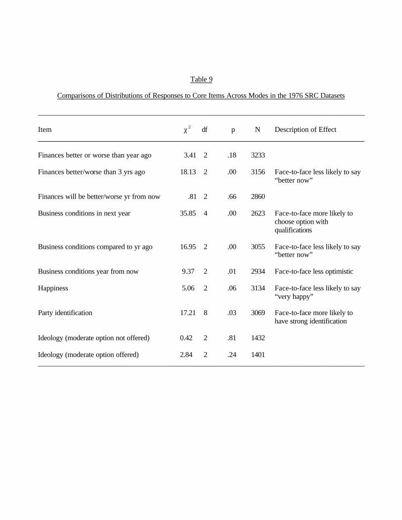
Table 9

Comparisons of Distributions of Responses to Core Items Across Modes in the 1976 SRC Datasets __________________________________________________________________________________________ Item χ2 df p N Description of Effect Finances better or worse than year ago 3.41 2 .18 3233 Finances better/worse than 3 yrs ago 18.13 2 .00 3156 Face-to-face less likely to say

“better now” Finances will be better/worse yr from now .81 2 .66 2860 Business conditions in next year 35.85 4 .00 2623 Face-to-face more likely to

choose option with qualifications

Business conditions compared to yr ago 16.95 2 .00 3055 Face-to-face less likely to say

“better now” Business conditions year from now 9.37 2 .01 2934 Face-to-face less optimistic Happiness 5.06 2 .06 3134 Face-to-face less likely to say

“very happy” Party identification 17.21 8 .03 3069 Face-to-face more likely to

have strong identification Ideology (moderate option not offered) 0.42 2 .81 1432 Ideology (moderate option offered) 2.84 2 .24 1401 _________________________________________________________________________________________

Table 10

Demographic Characteristics of the 2000 NES Telephone and Face-to-face Samples and the Nation ________________________________________________________________________________

2000 NES 2000 Current Demographic Telephone Face-to-Face Population Survey Education Less than high school diploma 9.0% 10.7% 16.9% High school diploma 26.6 30.4 32.8 More than high school or 2 year degree 30.5 29.9 27.1 Four year degree or more 33.5 28.6 23.2 TOTAL 99.5% 99.7% 100.0% N 797 1003 97,217 Average error 7.0 4.0 Income Less than $15,000 11.7% 15.0% 11.8% $15,000 to $24,999 9.6 10.8 12.0 $25,000 to $34,999 11.7 11.2 11.9 $35,000 to $49,999 15.0 12.8 16.1 $50,000 to $64,999 11.7 10.5 13.5 $65,000 to $74,999 6.7 7.1 6.9 $75,000 or above 19.6 20.5 27.9 TOTAL 86.1% 88.0% 100.0% N 690 885 97,217 Average error 2.0 2.6 Race White 79.5% 75.1% 83.3% Non-white 18.5 23.5 16.7 TOTAL 98.0% 98.6% 100.0% N 785 992 97,217 Average error 2.8 7.5 Gender Male 41.3% 44.4% 48.0% Female 58.7 55.6 52.0 TOTAL 100.0% 100.0% 100.0% N 801 1006 97,217

Average error 6.7 3.6 Age 18-24 years 6.7% 9.1% 13.1% 25-29 6.6 8.0 9.1 30-39 22.1 21.2 20.7 40-49 22.6 20.7 20.9 50-59 19.9 16.1 14.7 60-64 5.4 6.0 5.2 65 and over 15.7 18.8 16.2 TOTAL 99.0% 99.8% 100.0% N 801 1004 97,217 Average error 2.6 1.5 ________________________________________________________________________________ TOTAL AVERAGE ERROR 3.6 3.0 ________________________________________________________________________________

Table 11

Cross-Tabulations Comparing Distributions of Responses to Core Items Across Modes in the 2000 NES

____________________________________________________________________________________________________________

Item χ2 df p N Description of Effect

Party identification 16.50 6 .01 1599 Face-to-face more Democratic

Clinton approval 12.46 3 .01 1558 Face-to-face approved more

Approval of Clinton’s handling of the economy 1.94 3 .59 1686

Approval of Clinton’s handling of foreign affairs 2.13 3 .55 1688

Congressional approval 5.23 3 .16 1550

Recall name of candidate for House race 9.92 1 .00 1803 Face-to-face less likely to say they recall a name

Economy better or worse than year ago 15.74 2 .00 1787 Face-to-face more likely to say worse

Economy will be better/worse yr from now 2.68 2 .26 1740

Finances better or worse than year ago .93 4 .92 923

Finances will be better/worse yr from now 4.29 2 .12 847 Face-to-face more likely to say better

US position in the world become stronger or weaker 9.47 2 .01 1777 Telephone more likely to say weaker

Abortion position 11.00 3 .01 1758 Face-to-face more opposed to abortion

Vote choice in the upcoming election 7.17 5 .21 1463

Vote choice in 1996 election 3.17 3 .37 1238

Days in the past week read daily newspaper 20.47 7 .01 1807 Face-to-face say read on fewer days

Care who wins the House election 1.87 3 .60 1800

____________________________________________________________________________________________________________

Table 12

Effect of Mode on Satisficing Indicators for Low and High Education Respondents

____________________________________________________________________________________________

Low Education High Education Cohen’s Cohen’s t-test N d t-test N d

____________________________________________________________________________________________ Study 1 Michigan & Berkeley No opinion t(403)=4.82 409 .48** t(1678)=5.52 1684 .27** Nondifferentiation t(404)=2.66 410 .26** t(1679)=3.44 1685 .17** Michigan No opinion t(343)=5.52 349 .60** t(1325)=5.10 1331 .28** Nondifferentiation t(344)=.87 350 .09 t(1326)=2.04 1332 .11* Study 2 No opinion t(674)=.92 680 .07 t(1943)=1.67 1949 .08* Nondifferentiation t(677)=2.01 683 .15* t(1947)=1.16 1953 .06 Acquiescence t(673)=.02 679 .00 t(1936)=1.80 1942 .08* Study 3

No opinion t(591)=3.91 597 .32** t(947)=6.52 953 .42**

Nondifferentiation t(578)=.86 584 .07 t(942)=1.38 948 .09 Acquiescence t(591)=1.27 597 .10+ t(947)=1.84 953 .12*

Interview Length t(591)=4.07 597 .33** t(946)=3.20 952 .21**

____________________________________________________________________________________________ Average

Using Berkeley & Michigan from Study 1 .20** .17** Using only Michigan from Study 1 .19** .16**

____________________________________________________________________________________________ + p<.10 * p<.05 ** p<.01