THE STUDY OF FLUID FLOWS AND HEAT TRANSFER NEAR A STAGNATION POINT IN

A NEWTONIAN FLUID

WONG SIN WEI

FACULTY OF SCIENCE UNIVERSITY OF MALAYA

KUALA LUMPUR

2012

THE STUDY OF FLUID FLOWS AND HEAT TRANSFER

NEAR A STAGNATION POINT IN

A NEWTONIAN FLUID

WONG SIN WEI

DISSERTATION SUBMITTED IN FULFILLMENT OF

THE REQUIREMENTS FOR THE DEGREE OF

MASTER OF SCIENCE

INSTITUTE OF MATHEMATICAL SCIENCES

FACULTY OF SCIENCE

UNIVERSITY OF MALAYA

KUALA LUMPUR

2012

UNIVERSITI MALAYA

ORIGINAL LITERARY WORK DECLARATION

Name of Candidate: WONG SIN WEI (I.C/Passport No: 870413-56-5034)

Registration/Matric No: SGP 100003

Name of Degree: MASTER OF SCIENCE

Title of Project Paper/Research Report/Dissertation/Thesis (“this Work”):

THE STUDY OF FLUID FLOWS AND HEAT TRANSFER NEAR A STAGNATION

POINT IN A NEWTONIAN FLUID

Field of Study: FLUID MECHANICS

I do solemnly and sincerely declare that:

(1) I am the sole author/writer of this Work;

(2) This Work is original;

(3) Any use of any work in which copyright exists was done by way of fair dealing and

for permitted purposes and any excerpt or extract from, or reference to or

reproduction of any copyright work has been disclosed expressly and sufficiently and

the title of the Work and its authorship have been acknowledged in this Work;

(4) I do not have any actual knowledge nor ought I reasonably to know that the making

of this work constitutes an infringement of any copyright work;

(5) I hereby assign all and every rights in the copyright to this Work to the University of

Malaya (“UM”), who henceforth shall be owner of the copyright in this Work and

that any reproduction or use in any form or by any means whatsoever is prohibited

without the written consent of UM having been first had and obtained;

(6) I am fully aware that if in the course of making this Work I have infringed any

copyright whether intentionally or otherwise, I may be subject to legal action or any

other action as may be determined by UM.

Candidate’s Signature Date

Subscribed and solemnly declared before,

Witness’s Signature Date

Name:

Designation:

ii

ABSTRAK

Aliran mantap dua dimensi bendalir likat tak mampat dan pemindahan haba sekitar

titik genangan bendalir Newtonan dikaji. Tiga jenis masalah aliran bendalir likat

dipertimbangkan. Masalah pertama ialah mengenai kesan daya keapungan ke atas aliran

sekitar titik genangan helaian mencancang yang meregang, sementara masalah kedua ialah

aliran bendalir likat di atas helaian mendatar yang mengecut atau meregang secara

eksponen. Dalam masalah ketiga, kajian terhadap aliran bendalir likat di atas helaian

mendatar yang mengecut atau meregang secara eksponen diperluaskan, dengan

mengambil kira pelesapan kelikatan dan pemindahan haba. Masalah ini dipengaruhi oleh

parameter tertentu, iaitu keapungan, eksponen halaju, sedutan atau suntikan, dan

keregangan atau kekecutan sempadan yang bergerak. Daripada tranformasi pembolehubah

keserupaan, sistem persamaan pembezaan separa (PPS) dijelmakan kepada sistem

persamaan pembezaan biasa (PPB). Penyelesaian sistem PPB diselesaikan secara

berangka melalui beza terhingga tengah Keller-box, yang menurunkan persamaan PPB

peringkat ketiga atau yang rendah kepada sistem PPB peringkat satu. Ciri-ciri aliran dan

pemindahan haba untuk nilai-nilai parameter yang berbeza dikaji dan dibincangkan.

Daripada penyelesaian ini, wujud dua penyelesaian yang bergantung kepada parameter-

parameter tertentu di mana selain penyelesaian aliran bendalir yang biasa terdapat pula

penyelesaian aliran terbalik.

iii

ABSTRACT

Two-dimensional steady, incompressible viscous fluid flows and heat transfer near

a stagnation point in Newtonian fluid are studied. Three different problems of fluid flows

are considered. In the first problem buoyancy force on stagnation point flow towards a

vertical stretching sheet is studied, whilst the second problem is about viscous fluid flow

over an exponentially shrinking or stretching horizontal sheet. In the third problem, the

study of viscous fluid flow over an exponentially stretching or shrinking sheet is extended

with the inclusion of viscous dissipation and mass transfer. These problems are governed

by certain parameters, namely buoyancy, velocity exponents, suction or injection, and

stretching or shrinking of the moving boundary. From similarity variables transformations,

the governing system of partial differential equations (PDEs) is transformed into a system

of ordinary differential equations (ODEs). The solutions of system of ODEs are computed

numerically by a central finite difference Keller-box method, which reduces third or lower

order ODE to a system of first-order ODEs. The flow features and heat transfer

characteristics for different values of the governing parameters are analyzed and

discussed. From these solutions, it was found that dual solutions exist at certain range of

parameters whereby apart from the normal fluid flow solutions, reverse flow solutions are

also obtained.

iv

ACKNOWLEDGEMENTS

First, I would like to express my deepest gratitude to my supervisors, Mr. Md. Abu

Omar Awang and Prof. Dr. Anuar Mohd. Ishak, for their guidance, support and patience

throughout the years of my post-graduate studies. Their intuition and insight in attacking a

problem always fascinated me and their enthusiasm, encouragement and devotion have

always been a source of inspiration to me.

A special thanks to my family. I couldn’t have reached this point without the

invaluable support provided by my family.

I would also like to say thank-you to all those who have supported me in any

respect during the life of my research. In fact, I am fortunate to meet those wonderful

people who have enriched my life.

Finally, my thanks to Institute of Mathematical Sciences, University of Malaya and

also Ministry of Higher Education Malaysia for their financial support for this research.

v

TABLE OF CONTENTS

ABSTRAK ii

ABSTRACT iii

ACKNOWLEDGEMENTS iv

TABLE OF CONTENTS v

LIST OF TABLES viii

LIST OF FIGURES ix

LIST OF SYMBOLS AND ABBREVIATIONS xii

CHAPTER 1 INTRODUCTION

1.1 Background of the Study 1

1.2 Basic Conservation Equation 2

1.2.1 Law of conservation of mass 3

1.2.2 Law of conservation of momentum 5

1.2.3 Law of conservation of energy 9

1.3 Derivation of Boundary Layer Equations 14

1.4 Similarity Transformation 19

1.5 Numerical Implementations 20

1.6 Layout of the Thesis 21

vi

CHAPTER 2 BUOYANCY FORCE ON STAGNATION-POINT FLOW

TOWARDS A VERTICAL, NON-LINEARLY STRETCHING

SHEET WITH PRESCRIBED SURFACE HEAT FLUX

2.1 Introduction 23

2.2 Problem Formulation 24

2.3 Results and Discussion 28

2.4 Conclusion 32

CHAPTER 3 STAGNATION POINT FLOW OVER AN EXPONENTIALLY

SHRINKING/STRETCHING SHEET

3.1 Introduction 33

3.2 Problem Formulation 35

3.3 Results and Discussion 38

3.4 Conclusion 45

CHAPTER 4 BOUNDARY LAYER FLOW AND HEAT TRANSFER

OVER AN EXPONENTIALLY STRETCHING/SHRINKING

PERMEABLE SHEET WITH VISCOUS DISSIPATION

4.1 Introduction 46

4.2 Problem Formulation 48

4.3 Results and Discussion 52

4.3.1 Stretching case, 1 53

4.3.2 Shrinking case, 1 56

vii

4.4 Conclusion 64

CHAPTER 5 CONCLUSIONS AND FUTURE WORK 65

REFERENCES 68

viii

LIST OF TABLES

Tables Page

4.1 Values of (0) for bifurcation points in Figures 4.9 and 4.10 59

ix

LIST OF FIGURES

Figure Page

1.1 Boundary layer at a flat plate 1

1.2 Stagnation point flow 2

1.3 Fluid particles in box fixed in space 4

1.4 Stresses on a control volume dxdydz in a fixed frame, only forces in x-direction

are shown. 7

2.1 Physical model and coordinate system 24

2.2 Variation of the skin friction coefficient (0)f with for various values of

m when 0.5 29

2.3 Variation of the skin friction coefficient (0)f with for various values of

m when 1 29

2.4 Variation of the local Nusselt number 1/ (0) with for various values of

m when 0.5 31

2.5 Variation of the local Nusselt number 1/ (0) with for various values of

m when 1 31

3.1 Physical model and coordinate system 35

3.2 Variation of the skin friction coefficient (0)f with 39

3.3 Variation of the local Nusselt number (0) with for various values of

Pr 40

3.4 Velocity profile ( )f for various values of 0 40

3.5 Temperature profile ( ) for various values of 0 when Pr = 1 41

3.6 Temperature profile ( ) for various values of Pr when 1.45 42

x

3.7 Temperature profile ( ) for various values of Pr when 0.5 43

3.8 Temperature profile ( ) for various values of when Pr = 1 43

3.9 Velocity profile ( )f for various values of 44

4.1 Physical model and coordinate system 48

4.2a Dimensionless stream function ( )f for various values of s when 1 52

4.2b Streamlines for 0s and 1 52

4.3 Variation of the skin friction coefficient (0)f with s when 1 53

4.4 Variation of the local Nusselt number (0) with s for various values of

Pr when 1 and Ec = 1 54

4.5 Variation of the local Nusselt number (0) with s for various values of

Ec when 1 and Pr = 1 54

4.6 Velocity profile ( )f for various values of s when 1 55

4.7 Temperature profile ( ) for various values of s when 1, Pr = 1

and Ec = 1 56

4.8 Variation of the skin friction coefficient (0)f with s when 1 57

4.9 Variation of the local Nusselt number (0) with s for various values of

Pr when 1 and Ec = 1 58

4.10 Variation of the local Nusselt number (0) with s for various values of

Ec when 1 and Pr = 1 59

4.11 Temperature ( ) variation, with 2.3s and Ec 1 , for various values of

Pr when 1 60

4.12 Temperature ( ) variation, with 2.3s and Pr 1 , for various values of

xi

Ec when 1 60

4.13 Velocity profile ( )f for various values of s when 1 61

4.14 Temperature profile ( ) for various values of s when 1,Pr 1

and 1Ec 62

4.15 Velocity profile ( )f when 3.5s for 1 63

4.16 Temperature profile ( ) for 1 when 3.5,Pr 1, 1s Ec 63

xii

LIST OF SYMBOLS AND ABBREVIATIONS

a, b, c constants

Cf skin friction coefficient

Cp specific heat of the fluid at constant pressure

Ec Eckert number

f dimensionless stream function

g acceleration due to gravity

Grx local Grashof number

k thermal conductivity

L reference length

m velocity exponent parameter

Nux local Nusselt number

Pr Prandtl number

qw surface heat flux

Rex local Reynolds number

s suction/injection parameter

T fluid temperature

T ambient temperature

Tw surface temperature

T0 constant sheet temperature

U free stream velocity

Uw velocity of the shrinking/stretching sheet

xiii

u, v velocity components along the x- and y- directions, respectively

x, y cartesian coordinates along the surface and normal to it, respectively

Greek Letters

thermal diffusivity

thermal expansion coefficient

ε stretching/shrinking parameter

similarity variable

dimensionless temperature

buoyancy parameter

dynamic viscosity

kinematic viscosity

fluid density

w surface shear stress

stream function

Subscripts

w condition at the solid surface

condition far away from the solid surface

Superscript

' differentiation with respect to

1

CHAPTER 1

INTRODUCTION

1.1 Background of the Study

Fluids, unlike solids, can deform continuously under a shear stress. Our interest in

this thesis is to study the flows that are dominated by viscosity and thermal diffusivity,

which are known as viscous flows. For a viscous flow over a flat plate, the fluid particles

tend to decelerate faster nearer the solid plate surface compared to the free stream, thus

creating a thin shear layer called boundary layer. This boundary layer is graphically

depicted in Figure 1.1.

Figure 1.1 Boundary layer at a flat plate

In this study, we are interested in seeing how the viscous action affects the

boundary layer thickness, the skin friction (drag force) and the heat transfer rate. We

restrict our attention to Newtonian fluid flows near a stagnation point. Here, Newtonian

fluids are fluids in which its shear stress is directly proportional to the rate of deformation

only. For example water, air and gasoline. Stagnation point is a point in the flow where the

2

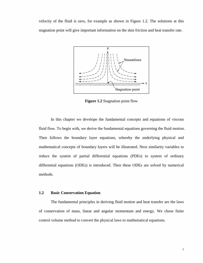
velocity of the fluid is zero, for example as shown in Figure 1.2. The solutions at this

stagnation point will give important information on the skin friction and heat transfer rate.

Figure 1.2 Stagnation point flow

In this chapter we develope the fundamental concepts and equations of viscous

fluid flow. To begin with, we derive the fundamental equations governing the fluid motion.

Then follows the boundary layer equations, whereby the underlying physical and

mathematical concepts of boundary layers will be illustrated. Next similarity variables to

reduce the system of partial differential equations (PDEs) to system of ordinary

differential equations (ODEs) is introduced. Then these ODEs are solved by numerical

methods.

1.2 Basic Conservation Equation

The fundamental principles in deriving fluid motion and heat transfer are the laws

of conservation of mass, linear and angular momentum and energy. We chose finite

control volume method to convert the physical laws to mathematical equations.

3

1.2.1 Law of conservation of mass

The law of conservation of mass of fluid particles can be derived by considering

moving fluid particles entering and leaving a box fixed in space, as shown in Figure 1.3.

The velocity components , u v and w of fluid particles are in the direction of , x y and z

respectively. The mass flow rate per unit area into the box in the x -direction is given by

u dydz , where is the density of the fluid, whilst the mass flow rate per unit area out

of the box in the x -direction is

x dx u x dx dydz

2 22 2

2 2... ...

2! 2!

dx dxu udx u dx dydz

x x x x

higher order terms

uu dx dydz

x

.

Therefore the net flow rate in the x -direction is u dxdydzx

. The same mass flow

rate per unit area are applied in the y -direction and z -direction respectively. Hence, the

net flow rate into the box dxdydz is

higher order termsu v w dxdydzx y z

. (1.1)

The mass increment per unit time of the fluid particles in this fixed box is

dx dy dz dx dy dzt t

. (1.2)

4

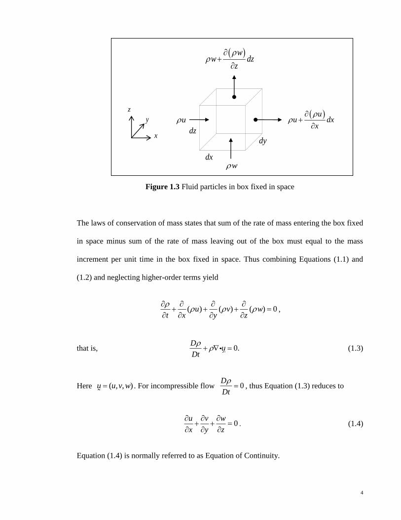
Figure 1.3 Fluid particles in box fixed in space

The laws of conservation of mass states that sum of the rate of mass entering the box fixed

in space minus sum of the rate of mass leaving out of the box must equal to the mass

increment per unit time in the box fixed in space. Thus combining Equations (1.1) and

(1.2) and neglecting higher-order terms yield

( ) ( ) ( ) 0u v wt x y z

,

that is, 0.D

uDt

(1.3)

Here ( , , )u u v w . For incompressible flow 0D

Dt

, thus Equation (1.3) reduces to

0u v w

x y z

. (1.4)

Equation (1.4) is normally referred to as Equation of Continuity.

ww dz

z

u

dz

z

y

x

uu dx

x

dx

dy

w

5

In two-dimensional flow independent of coordinate z , Equation (1.4) becomes

0u v

x y

. (1.5)

1.2.2 Law of conservation of momentum

According to the laws of conservation of momentum, which is also called

Newton’s second law, mass ( )m times acceleration ( )a is equal to sum of the applied

forces. In viscous flow, there are two types of forces to be considered, which are body

forces (pressure) and surface forces (friction forces). The body forces act on every fluid

particle of the body whereas the surface forces acts on the fluid surface element only, and

these create the deformation of the fluid. If bf is the body force per unit volume, sf the

surface force per unit area, and F is the sum of all body and surface forces, the

relationship for the momentum equation in a control volume dxdydz is

; = b sF ma F f f . (1.6)

Recall that the mass of the fluid particles in a control volume dxdydz in a fixed frame of

reference is

m dx dy dz , (1.7)

and the acceleration of the fluid particles in Cartesian coordinate is

Dua

Dt

uu u

t

(1.8)

6

where D Dt is the material derivative, u t is local acceleration and u u is the

convective acceleration. Therefore, the acceleration field in , x y and z direction

respectively will be

,

,

.

Du u u u uu v w

Dt t x y z

Dv v v v vu v w

Dt t x y z

Dw w w w wu v w

Dt t x y z

(1.9)

In order to determine the surface forces, consider the diagram shown in Figure 1.4.

Stresses are defined as surface forces per unit surface area. Normal stresses are stress

components that act perpendicularly to surface of control volume dxdydz , while tangential

(shear) stresses are the components in the plane of the surface of control volume

dxdydz . The surface forces can be expressed as follows:

in the direction: ,xyxx xzx dx dy dz

x y z

in the direction: ,yx yy yz

y dx dy dzx y z

(1.10)

in the direction: .

zyzx zzz dx dy dzx y z

7

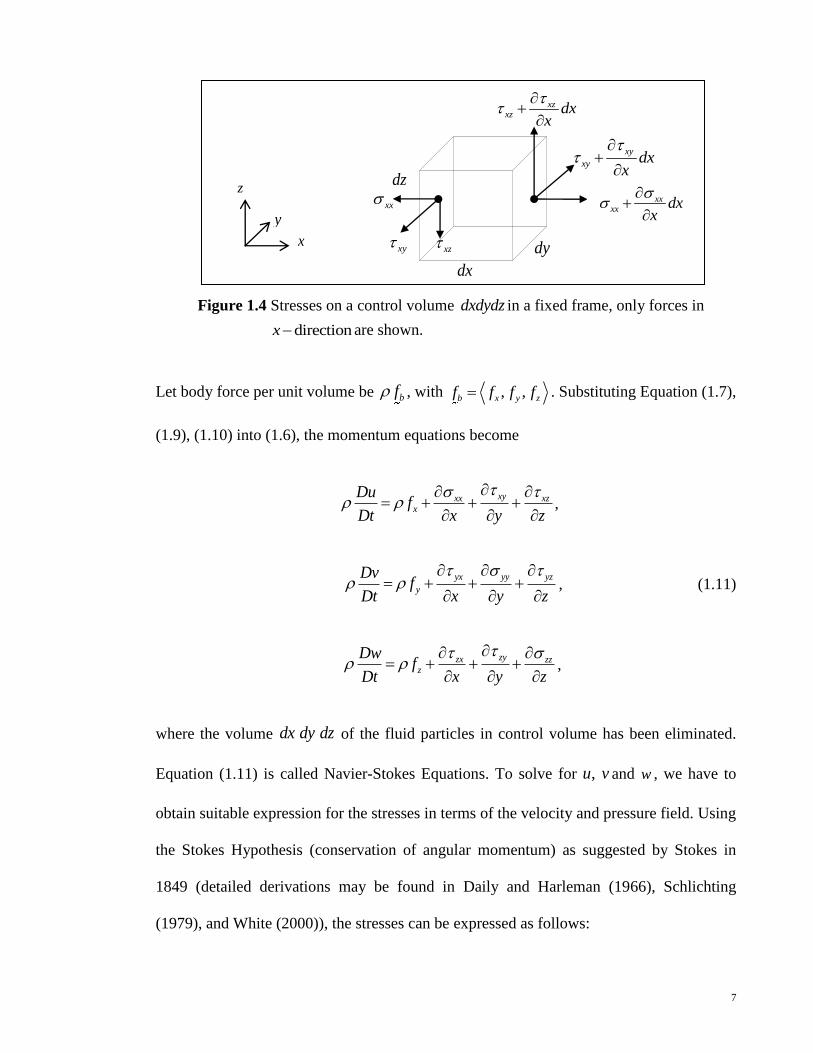
Figure 1.4 Stresses on a control volume dxdydz in a fixed frame, only forces in

directionx are shown.

Let body force per unit volume be bf , with , ,b x y zf f f f . Substituting Equation (1.7),

(1.9), (1.10) into (1.6), the momentum equations become

xyxx xzx

Duf

Dt x y z

,

yx yy yz

y

Dvf

Dt x y z

, (1.11)

zyzx zzz

Dwf

Dt x y z

,

where the volume dx dy dz of the fluid particles in control volume has been eliminated.

Equation (1.11) is called Navier-Stokes Equations. To solve for , u v and w , we have to

obtain suitable expression for the stresses in terms of the velocity and pressure field. Using

the Stokes Hypothesis (conservation of angular momentum) as suggested by Stokes in

1849 (detailed derivations may be found in Daily and Harleman (1966), Schlichting

(1979), and White (2000)), the stresses can be expressed as follows:

xz xy

xzxz dx

x

xy

xy dxx

xx

dz z

y

x

xxxx dx

x

dx

dy

8

xy

v u

x y

,

yz

w v

y z

,

zx

u w

z x

, (1.12)

22

3xx

up u

x

,

22

3yy

vp u

y

,

2

23

zz

wp u

z

,

where is viscosity of the fluid, is gradient operator and .u v w

ux y z

p is

the local thermodynamic pressure, defined as 3xx yy zzp . Substituting

Equation (1.12) into (1.11), we obtain

22

3x

Du p u u v w uf u

Dt x x x y y x z x z

,

22

3y

Dv p v u v v wf u

Dt y y y x y x z z y

, (1.13)

22

3z

Dw p w w u w wf u

Dt z z z x x z y z y

.

These equations are the complete Navier-Stokes equations for three-dimensional, unsteady,

and compressible viscous flow in Cartesian coordinates.

9

If viscosity is constant and u is zero i.e the fluid is incompressible, Equation (1.13)

is significantly reduced to

2 2 2

2 2 2 x

u u u u p u u uu v w f

t x y z x x y z

,

2 2 2

2 2 2 y

v v v v p v v vu v w f

t x y z y x y z

,

2 2 2

2 2 2 z

w w w w p w w wu v w f

t x y z z x y z

,

2

b

Dup u f

Dt . (1.14)

For steady, two-dimensional compressible flow Equation (1.14) becomes

2 2

2 2 x

u u p u uu v f

x y x x y

, (1.15)

2 2

2 2 y

v v p v vu v f

x y y x y

. (1.16)

1.2.3 Law of conservation of energy

The equation for the conservation of energy can be deduced using the same

approach as used when deriving the momentum equations. The first law of

thermodynamics states that sum of the heat supplied and the work done on the fluid

particles in a control volume dxdydz is equal to the total energy gained in unit time, that is

10

DE

Q WDt

, (1.17)

where E is the total energy, Q is the heat supplied and W is the work done on the fluid.

Let heat flux vector , ,x y zq q q q denotes the heat transferred per unit surface area. The

heat entering the box fixed in space in the directionx is xq dy dz and the heat

transferred out of the box is x xq q x dx dy dz . Therefore, the net total heat flux

transferred in x -direction is x xQ q x dx dy dz . The same applies in the y and

z direction. Thus, the total heat supply is

. ,

yx zqq q

Q dx dy dzx y z

q dV

(1.18)

where dV dxdydz . Assuming small temperature differences, from Fourier (1822) heat

law, the heat conduction for the fluid is

, , x y z

T T Tq k q k q k

x y z

,

that is, ,q k T (1.19)

where the thermal conductivity k is a positive physical property. Thus, Equation (1.18)

becomes

.

T T TQ k k k dx dy dz

x x y y z z

k T dV

. (1.20)

11

Next, we derived the work done W on the fluid. Work done W on a moving fluid

particle in a fixed box is equal to the product of its velocity and the component of the

stress forces in the direction of velocity. Hence work done on moving fluid particles by

the stress forces in the x direction is simply the velocity in the x direction u multiply by

the stress forces. With the aid of Figure (1.4), work done by the stress forces on the

surface dydz of control volume dxdydz in the x direction is

( ) ( ) higher order term

( ) ( ) higher order term

( ) ( ) higher order term

xx

xx xx

xy

xy xy

xz

xz xz

uu x dx x dx dydz u dx dydz

x

uu y dy y dy dxdz u dy dxdz

y

uu z dz z dz dxdy u dz dxdy

z

(1.21)

Neglecting the higher order terms, the net work done by the stress forces acting in the x

direction is

xyxx

xx xx xy xy

xz

xz xz

xyxx xz

uuu dx u dydz u dy u dxdz

x y

uu dz u dxdy

z

uu udxdydz

x y z

(1.22)

12

The net work done by stress forces in the y and z directions can be obtained in a similar

manner, that is

in the direction: ,

in the direction: .

xy yy yz

zyxz zz

v v vy dx dy dz

x y z

ww wz dx dy dz

x y z

(1.23)

Combining and rearranging these results, the total work done in control volume dxdydz is

xx xy xz yy yx yz zz zx zyW u v w v u w w u v dxdydzx y z

. (1.24)

Using Stokes’ Hypothesis (1.12) into the work done, we obtained

22

3

22

3

xx xy xz yy yx yz zz zx zyu v w v u w w u vx y z

u u v w v u w uu v w

x x x y z x y x z

v u v w uv u

y y x y z y

22

3

v w vw

x y z

w u v w u w v ww u v

z z x y z z x z y

(1.25)

Finally, the total energy E per unit time is the sum of the internal energy ( e ) and

kinetic energy (21

2u ). This is given by

212

( )

D e uDEdx dy dz

Dt Dt

. (1.26)

13

Substituting Equation (1.20), (1.24) and (1.25) into (1.17), we obtain the general form of

the energy equation.

However, from thermodynamics, the energy equation can also be expressed in

terms of enthalpy h by

ph e

. (1.27)

By using the general relation as suggested by Kestin (1966),

1

p

Dh DT T Dpc

Dt Dt Dt

, (1.28)

where pc is the specify heat capacity at constant pressure and

1

pT

is the

coefficient of thermal expansion, the energy equation can thus be rewritten as

p

DT T T T Dpc k k k T

Dt x x y y z z Dt

, (1.29)

where is the viscous dissipation function, defined as

2 2 22 2

22

2

2 .

3

u v w v u w v

x y z x y y z

u w u v w

z x x y z

(1.30)

14

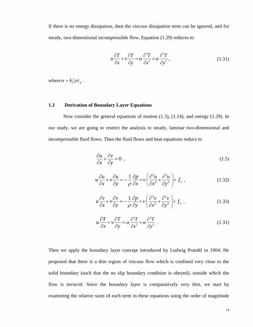
If there is no energy dissipation, then the viscous dissipation term can be ignored, and for

steady, two-dimensional incompressible flow, Equation (1.29) reduces to

2 2

2 2

T T T Tu v

x y x y

, (1.31)

where pk c .

1.3 Derivation of Boundary Layer Equations

Now consider the general equations of motion (1.3), (1.14), and energy (1.29). In

our study, we are going to restrict the analysis to steady, laminar two-dimensional and

incompressible fluid flows. Then the fluid flows and heat equations reduce to

0u v

x y

, (1.5)

2 2

2 2

1x

u u p u uu v f

x y x x y

, (1.32)

2 2

2 2

1y

v v p v vu v f

x y y x y

, (1.33)

2 2

2 2

T T

x y

T Tu v

x y

. (1.31)

Then we apply the boundary layer concept introduced by Ludwig Prandtl in 1904. He

proposed that there is a thin region of viscous flow which is confined very close to the

solid boundary (such that the no slip boundary condition is obeyed), outside which the

flow is inviscid. Since the boundary layer is comparatively very thin, we start by

examining the relative sizes of each term in these equations using the order of magnitude

15

argument. As a typical illustration, consider the flow past a horizontal plate. Let the x -

axis lie along the horizontal plane and y -axis perpendicular to it. Let be the thickness

of the boundary layer where 1 , l is the length of the plate and also is (1)O , and u is

the velocity that varies from 0 at the solid surface to U of the main stream. Therefore

( ), ( ), ( )x O l y O u O U . (1.34)

From the continuity equation (1.5), their order of magnitudes is;

0u v

x y

,

, U v

O Ol

. (1.35)

Since both terms in the equation are of the same order of magnitude, the magnitude of

velocity v is ( / )O U l .

Now, examine the order of magnitude of Equation (1.32), and relegating the body

force xf to later consideration, we see that

2 2

2 2 ,

1

u u p u uu v

x y x x y

gives

2

2 2

1 , = , ,

U U U U U UO U O O O O

l l l l

.

Multiplying by 2

l

U

, this becomes

2

1 , 1 = 1 , , l

O O O O OU l U l

(1.36)

16

Now the term 2 2/u x can be neglected when compared with the term

2 2/u y , because

22 2

2 21.

u uO

x y l

(1.37)

Since the diffusion term 2 2/u y must have an order of magnitude of (1)O , we see

that

12

1/2

Re 1,l

O O lU

(1.38)

where Reynolds number Re 1.U l

Hence, Equation (1.32) now becomes

2

2

1 u

y

u u pu v

x y x

, (1.39)

in the limit R .

Similarly, postponing the discussion on body force yf , the order of magnitude for

Equation (1.33) is;

2 2

2 2 2

2 2

2 2 ,

1 , = , ,

1

1U U U U UO U O O O O

l l l l

v v p v vu v

x y y x y

Multiply by 2U

,

17

2 2 2

2 2 2 , = 1 , , O O O O O

l l U l U l

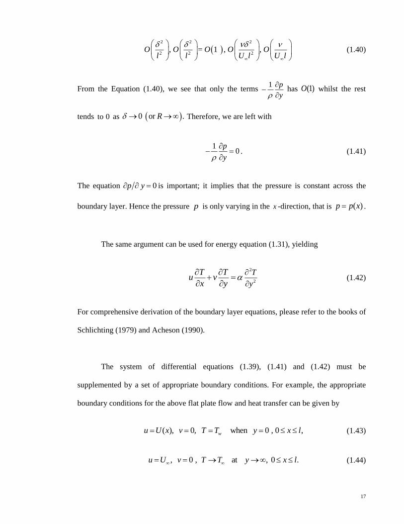
(1.40)

From the Equation (1.40), we see that only the terms 1 p

y

has (1)O whilst the rest

tends to 0 as 0 or .R Therefore, we are left with

1

0p

y

. (1.41)

The equation 0p y is important; it implies that the pressure is constant across the

boundary layer. Hence the pressure p is only varying in the x -direction, that is ( )p p x .

The same argument can be used for energy equation (1.31), yielding

2

2

T

y

T Tu v

x y

(1.42)

For comprehensive derivation of the boundary layer equations, please refer to the books of

Schlichting (1979) and Acheson (1990).

The system of differential equations (1.39), (1.41) and (1.42) must be

supplemented by a set of appropriate boundary conditions. For example, the appropriate

boundary conditions for the above flat plate flow and heat transfer can be given by

( ), 0, when 0 , 0 ,wu U x v T T y x l (1.43)

, 0 , at , 0 .u U v T T y x l (1.44)

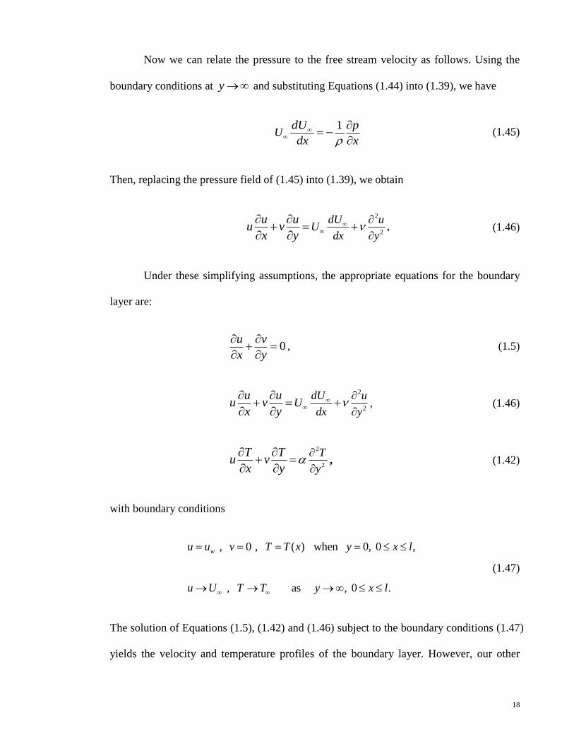
18

Now we can relate the pressure to the free stream velocity as follows. Using the

boundary conditions at y and substituting Equations (1.44) into (1.39), we have

1

UdU p

dx x

(1.45)

Then, replacing the pressure field of (1.45) into (1.39), we obtain

2

2

dU uU

dx y

u uu v

x y

. (1.46)

Under these simplifying assumptions, the appropriate equations for the boundary

layer are:

0u v

x y

, (1.5)

2

2

dU uU

dx y

u uu v

x y

, (1.46)

2

2

T

y

T Tu v

x y

, (1.42)

with boundary conditions

, 0 , ( ) when 0, 0 ,

, as , 0 .

wu u v T T x y x l

u U T T y x l

(1.47)

The solution of Equations (1.5), (1.42) and (1.46) subject to the boundary conditions (1.47)

yields the velocity and temperature profiles of the boundary layer. However, our other

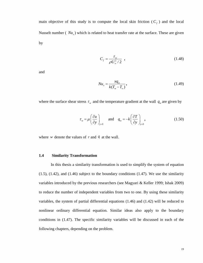
19

main objective of this study is to compute the local skin friction ( fC ) and the local

Nusselt number ( xNu ) which is related to heat transfer rate at the surface. These are given

by

2

/ 2

wfC

U

, (1.48)

and

( )

wx

w

xqNu

k T T

, (1.49)

where the surface shear stress w and the temperature gradient at the wall wq are given by

0 0

and w w

y y

u Tq k

y y

, (1.50)

where w denote the values of and q at the wall.

1.4 Similarity Transformation

In this thesis a similarity transformation is used to simplify the system of equation

(1.5), (1.42), and (1.46) subject to the boundary conditions (1.47). We use the similarity

variables introduced by the previous researchers (see Magyari & Keller 1999; Ishak 2009)

to reduce the number of independent variables from two to one. By using these similarity

variables, the system of partial differential equations (1.46) and (1.42) will be reduced to

nonlinear ordinary differential equation. Similar ideas also apply to the boundary

conditions in (1.47). The specific similarity variables will be discussed in each of the

following chapters, depending on the problem.

20

1.5 Numerical Implementations

In this research, we have used an efficient and accurate finite difference scheme,

Keller-box method, to solve the system of nonlinear ODEs subject to the appropriate

boundary conditions. This method was first suggested by Keller (1970). Its

implementation is described in Keller and Cebeci (1971, 1972). An interesting feature of

this method is that it is unconditionally stable and is second order accurate. Several

authors for instance Ishak et al. (2007, 2009a), Ali et al. (2011), Saha et al. (2007) and Yih

(1998) have successfully used this method to solve various fluid flow and heat transfer

problems.

The basic idea of the Keller-box method is:

(i) First, introduce new dependent variables and reduce the system of nonlinear ODE

to a first-order system of ODEs.

(ii) Replace the derivatives of the first order system of ODEs by central differences.

(iii) Linearize the resulting algebraic equations by Newton’s method, and write them in

matrix-vector form.

(iv) The linearized difference equations are solved by the block tridiagonal elimination

technique (Thomas method).

In our calculations, we have used step size = 0.001 with a convergence

criterion of error less than 10-6

. The location of the edge of the boundary layer has

been adjusted appropriately for different values of parameters to maintain the necessary

accuracy. For all the problems discussed, MATLAB has been used for coding.

21

1.6 Layout of the Thesis

In Chapter 2, 3, and 4 we are going to discuss specific boundary layer problems.

The relevant conclusions will be presented at the end of each chapter. These are part of

published and unpublished results.

In Chapter 2, we consider the two- dimensional stagnation point flow past a

vertical sheet. The sheet is stretched non-linearly; with the velocity and prescribed surface

heat flux in power law form. We give a lot of consideration to the effect of buoyancy force

and velocity ratio toward the boundary layer problems. Both assisting and opposing

buoyant flows are considered. Our results show that assisting buoyant flow has unique

solution whilst an increase in velocity ratio leads to an increase in the solution range.

In Chapter 3 the two-dimensional stagnation-point flow due to shrinking or

stretching sheet is studied. Here, the shrinking or stretching velocity, the free stream

velocity and the surface temperature are in an exponential form, which is different from

those in Chapter 2. We investigate the existence and (non)uniqueness of solutions, for

both shrinking and stretching sheet. Our results indicate that the solutions in shrinking

sheet are not unique.

In Chapter 4, we extend the problem of Chapter 3 by the inclusion of mass transfer

and viscous forces. Therefore in this chapter we discuss the two-dimensional stagnation-

point flow over an exponentially stretching or shrinking permeable sheet with the

additional effects of viscous forces and mass transfer. Our numerical results show that in

shrinking boundary layer with wall injection no solution will exist.

22

In our last chapter, Chapter 5, we present the summary of our research. The

conclusions, suggestions or recommendations are discussed in this chapter.

23

CHAPTER 2

BUOYANCY FORCE ON STAGNATION-POINT FLOW TOWARDS A

VERTICAL, NON-LINEARLY STRETCHING SHEET WITH PRESCRIBED

SURFACE HEAT FLUX

2.1 Introduction

The study of stagnation point fluid flow and heat transfer due to a nonlinearly

stretching surface has significant application in the industrial processes. For example hot

metal plate in a cooling bath, production of metal or polymer sheet and manufacturing of

glass fiber. The quality of the final product greatly depends on the heat transfer at the

stretching surface as explained by Karwe and Jaluria (1988, 1991).

Our objective is to discuss the flow and heat transfer characteristics that are

brought about by buoyancy force towards a vertical stretching sheet. Several works that

have been reported in this type of flow field (Gupta & Gupta 1977; Nazar et al. 2004;

Chen 1998). Ramachandran et al. (1988) studied the effect of buoyancy force on the

stagnation point flows past a vertically heated surface at rest and found that dual solutions

exist in the buoyancy opposing flow region. Ishak et al. (2008a) extended the idea of

Ramachandran (1988) to the fluid induced by the velocity ratio parameter. Ishak et al.

(2009a) also considered unsteady flow along stretching sheet and showed that

unsteadiness parameter increases the solution range. Moreover, Ishak et al. (2008b, 2008c)

have numerically studied the flow induced by stretching vertical sheet in micropolar fluid

and MHD fluid.

24

Motivated by the above investigations, in this research we study the stagnation-

point flow towards a nonlinearly stretching sheet with prescribed surface heat flux. The

stretching velocity, the free stream velocity and the surface heat flux are assumed to vary

in the power-law form.

2.2 Problem Formulation

Consider a mixed convection stagnation-point flow towards a vertical nonlinearly

stretching sheet immersed in an incompressible viscous fluid, as shown in Figure 2.1. The

Cartesian coordinates ( yx, ) are taken such that the x axis is measured along the sheet

oriented in the upwards or downwards direction and the y axis is normal to it.

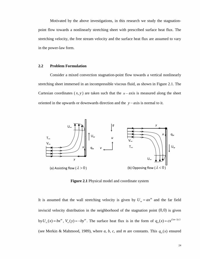
Figure 2.1 Physical model and coordinate system

It is assumed that the wall stretching velocity is given by m

wU ax and the far field

inviscid velocity distribution in the neighborhood of the stagnation point (0,0) is given

by ( ) mU x bx , ( ) mV y by . The surface heat flux is in the form of (5 3)/2( ) m

wq x cx

(see Merkin & Mahmood, 1989), where a, b, c, and m are constants. This ( )wq x ensured

T∞

T∞ V∞

V∞

U∞

U∞

Uw

Uw

(a) Assisting flow ( 0 ) (b) Opposing flow ( 0 )

y

x

y

x

g

u

v

qw

qw

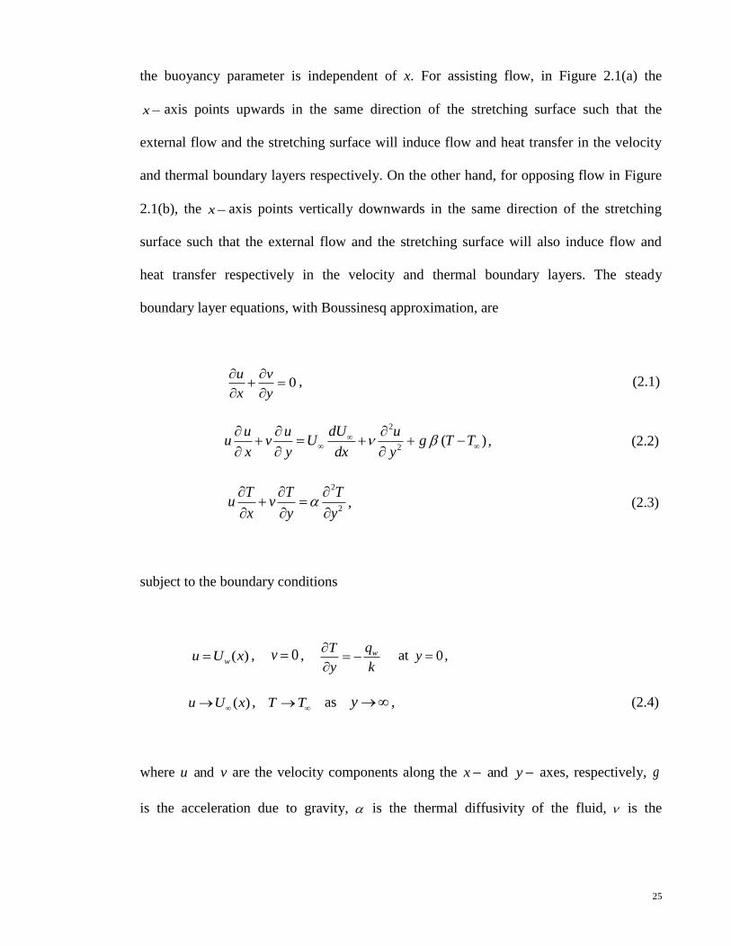
25

the buoyancy parameter is independent of x. For assisting flow, in Figure 2.1(a) the

x axis points upwards in the same direction of the stretching surface such that the

external flow and the stretching surface will induce flow and heat transfer in the velocity

and thermal boundary layers respectively. On the other hand, for opposing flow in Figure

2.1(b), the x axis points vertically downwards in the same direction of the stretching

surface such that the external flow and the stretching surface will also induce flow and

heat transfer respectively in the velocity and thermal boundary layers. The steady

boundary layer equations, with Boussinesq approximation, are

0

u v

x y

, (2.1)

2

2( )

dUu u uu v U g T T

x y dx y

, (2.2)

2

2

T T Tu v

x y y

, (2.3)

subject to the boundary conditions

( )wu U x , 0v , wqT

y k

at 0y ,

( )u U x , T T as y , (2.4)

where vu and are the velocity components along the yx and axes, respectively, g

is the acceleration due to gravity, is the thermal diffusivity of the fluid, is the

26

kinematic viscosity, is the coefficient of thermal expansion and is the fluid density.

T is the far field ambient constant temperature.

The continuity equation (2.1) can be satisfied automatically by introducing a

stream function such that /u y and /v x . The momentum and energy

equations are transformed by the similarity variables

1/ 2U

yx

, 1/ 2

( )xU f ,

1/2( )

( )w

k T T U

q x

(2.5)

into the following nonlinear ordinary differential equations:

211 0

2

mf ff m f

, (2.6)

1 1

(2 1) 0Pr 2

mf m f

. (2.7)

Here primes denote differentiation with respect to , 5/2/ Rex xGr is the buoyancy or

mixed convection parameter, Pr / is the Prandtl number, 4 2/ ( )x wGr g q x k is the

local Grashof number and Re /x U x is the local Reynolds number. We note that is

a constant, with 0 corresponds to assisting flow and 0 denote opposing flow

whilst 0 is for forced convective flow.

27

The transformed boundary conditions are

(0) 0f , (0)f , (0) 1 ,

( ) 1f , ( ) 0 as , (2.8)

where /a b .

The physical quantities of interest are the skin friction coefficient fC and the local

Nusselt number xNu , which are defined as

2

,/ 2

wfC

U

( )

wx

w

xqNu

k T T

(2.9)

respectively, where the surface shear stress w and the surface heat flux

wq are given by

0

,w

y

u

y

0

w

y

Tq k

y

(2.10)

with and k being the dynamic viscosity and thermal conductivity, respectively. Using

the non-dimensional variables (2.5), we obtain

1/21Re (0),

2f xC f

1/2

1

Re (0)

x

x

Nu

. (2.11)

28

2.3 Results and Discussion

Equations (2.6) and (2.7) subject to the boundary conditions (2.8) are integrated

numerically using a finite difference scheme known as the Keller box method (Keller

1970). Numerical results are presented for different physical parameters. To conserve

space, we consider Prandtl number unity throughout this paper. The results presented here,

whenever it is comparable, agree very well with those of Ramachandran et al. (1988).

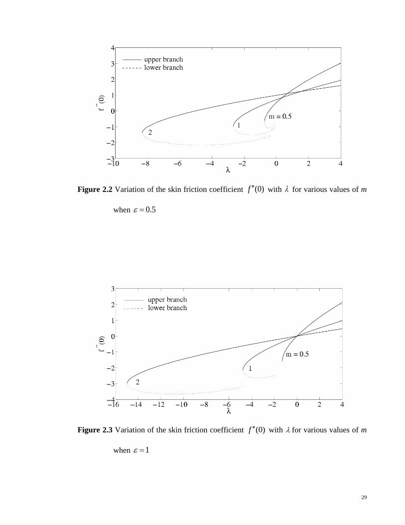
Figures 2.2 and 2.3 show the skin friction coefficient (0)f against buoyancy

parameter for some values of velocity exponent parameter m for velocity ratio

parameter 0.5 and 1 . Two branches of solutions are found. The solid lines are the

upper branch solutions and the dash lines are the lower branch solutions. With increasing

m , the dual solutions’ range increases. Also from both figures of the upper branch

solutions, the skin friction is higher for assisting buoyancy flow ( 0 ) compared to the

opposing flow ( 0 ). This implies that increasing buoyancy convection parameter

increases the skin friction coefficient (0)f . Whilst for 1 the values of (0)f in

Figure 2.3 are positive for 0 and negative for 0 . Physically, this means positive

(0)f implies the fluid exerts a drag force on the sheet and negative implies the reverse.

Similarly this also happens for 0.5 but at different values of .

29

Figure 2.2 Variation of the skin friction coefficient (0)f with for various values of m

when 0.5

Figure 2.3 Variation of the skin friction coefficient (0)f with for various values of m

when 1

30

As seen in Figures 2.2 and 2.3, there exist a critical value of buoyancyc such that

for c

there will be no solutions, for 0c there will be dual solutions, and when

0 the solution is unique. Our numerical calculations in Figure 2.2 shows that for

velocity ratio 0.5 c -8.331, -2.677 and -0.7411 for m 2, 1 and 0.5 respectively,

while in Figure 2.3 for velocity ratio 1 , c -14.98, -4.764 and -1.301 for m 2, 1 and

0.5 respectively. The dual solutions exhibit the normal forward flow behavior and also the

reverse flow where ( ) 0f . From these two results, it seems that an increase in velocity

ratio parameter leads to an increase of the critical values of | |c . This increases the dual

solutions range of Equations (2.6)-(2.8).

Figures 2.4 and 2.5 display the variations of the local Nusselt number 1/ (0)

against buoyant parameter , for some values of m when velocity ratio 0.5 and 1

respectively. Both figures clearly show that the local Nusselt number increases as

m increases for the upper branch solutions. For the lower branch solutions, the local

Nusselt number becomes unbounded as 0 . Positive values of 1/ (0) denote that

heat is being transferred from the sheet to the fluid, and vice versa.

31

Figure 2.4 Variation of the local Nusselt number 1/ (0) with for various values of m

when 0.5

Figure 2.5 Variation of the local Nusselt number 1/ (0) with for various values of m

when 1

32

2.4 Conclusions

The problem of mixed convective stagnation-point flow towards a nonlinearly

stretching vertical sheet immersed in an incompressible viscous fluid was investigated

numerically. The effects of the governing parameters m, and on the fluid flow and

heat transfer characteristics were discussed. It was found that for assisting flow, the

solution is unique, while dual solutions were found to exist for opposing flow up to a

certain critical value c . Moreover increasing the velocity exponent parameter m, the

solution range of Equations (2.6) –(2.8) increases.

33

CHAPTER 3

STAGNATION-POINT FLOW OVER AN EXPONENTIALLY

SHRINKING/STRETCHING SHEET

3.1 Introduction

Started from early of the last century, there have been numerous sophisticated

studies on boundary layer flow. The effects of viscosity and thermal conductivity are

important in this layer. Thus, this leads to an urge to understand the underlying physical,

mathematical and modeling concepts inherent in boundary layer. In reality, a majority of

the applications for the industrial manufacturing processes have to deal with fluid flow

and heat transfer behaviors. Examples include the polymer sheet extrusion from a dye,

gaseous diffusion, heat pipes, drawing of plastic film and etc. Such processes play an

important role to determine the quality of the final products as described by Karwe and

Jaluria (1988, 1991).

Crane (1970) was the first person who initiated the study of two-dimensional

steady flow of an incompressible viscous fluid induced by a linearly stretching plate. The

boundary layer equations were simplified using a similarity transformation, which

transformed the governing partial differential equations to a single ordinary differential

equation. Since then, there were similar flows that have been considered by several

researchers (Andersson et al. 1992; Gupta & Gupta 1977; Nazar et al. 2004; Hossain &

Takhar 1996; Ishak et al. 2006a). Such similar flows have been studied extensively in

various forms, for example flows with suction/injection, stretching, MHD effect, radiation

or non-Newtonian fluids. Magyari and Keller (1999) reported the similarity solutions

34

describing the steady plane (flow and thermal) boundary layers on an exponentially

stretching continuous surface with an exponential temperature distribution. This problem

was then extended by Bidin and Nazar (2009), Sajid and Hayat (2008) and Nadeem et al.

(2010a, 2010b) to include the effect of thermal radiation, while Pal (2010) and Ishak

(2011) studied the similar problem but in the presence of magnetic field. Sanjayanand and

Khan (2006) studied the heat and mass transfer in a viscoelastic boundary layer flow over

an exponentially stretching sheet. The mixed convection flow of a micropolar fluid over

an exponentially stretching sheet was considered by El-Aziz (2009). The problems in non-

Newtonian fluids considered in Sanjayanand and Khan (2006) and El-Aziz (2009) do not

admit similarity solutions, and thus the authors reported local similarity solutions with

certain assumptions.

Recently, the shrinking aspect has become a brand new topic. The abnormal

behavior in the fluid flow due to a shrinking sheet has gained attention from several

researchers. However, the work on it is relatively little. The flow induced by a shrinking

sheet was first discussed by Miklavčič and Wang (2006), where the existence and

(non)uniqueness of solutions in both numerical and exact solutions were proven.

Extension to that, Fang (2008) carried out the shrinking problem to power law surface

velocity with mass transfer. It was shown that the solution only exist with mass suction for

the rapidly shrinking sheet problem. Furthermore, Wang (2008) has investigated that the

shrinking sheet problem has many unique characteristics. Later on, Sajid et al. (2008)

studied the MHD rotating flow over a shrinking surface. It was found that the results in the

case of hydrodynamic flow are not stable for the shrinking surface and only meaningful in

the presence of magnetic field. The flow over a shrinking sheet in a porous medium was

studied by Nadeem and Awais (2008). On the other hand, Ishak et al. (2010a) solved

35

numerically micropolar fluid flow over a linearly shrinking sheet, and found that the

solutions are not unique in shrinking sheet. Very recently, Nadeem et al. (2009, 2010a,

2010b) studied the stagnation point flow over a shrinking sheet in non-Newtonian fluids.

Motivated by the above investigations, here we study the steady two dimensional

stagnation point flow over an exponentially shrinking/stretching sheet. The shrinking/

stretching velocity, the free stream velocity and the surface temperature are assumed to

vary in an exponential form with the distance from the stagnation point. The skin friction

coefficient and the local Nusselt number are determined for the understanding of the flow

and heat transfer characteristics. The practical applications include the cooling of extruded

materials in industrial processes using an inward directed fan or conical liquid jets.

3.2 Problem Formulation

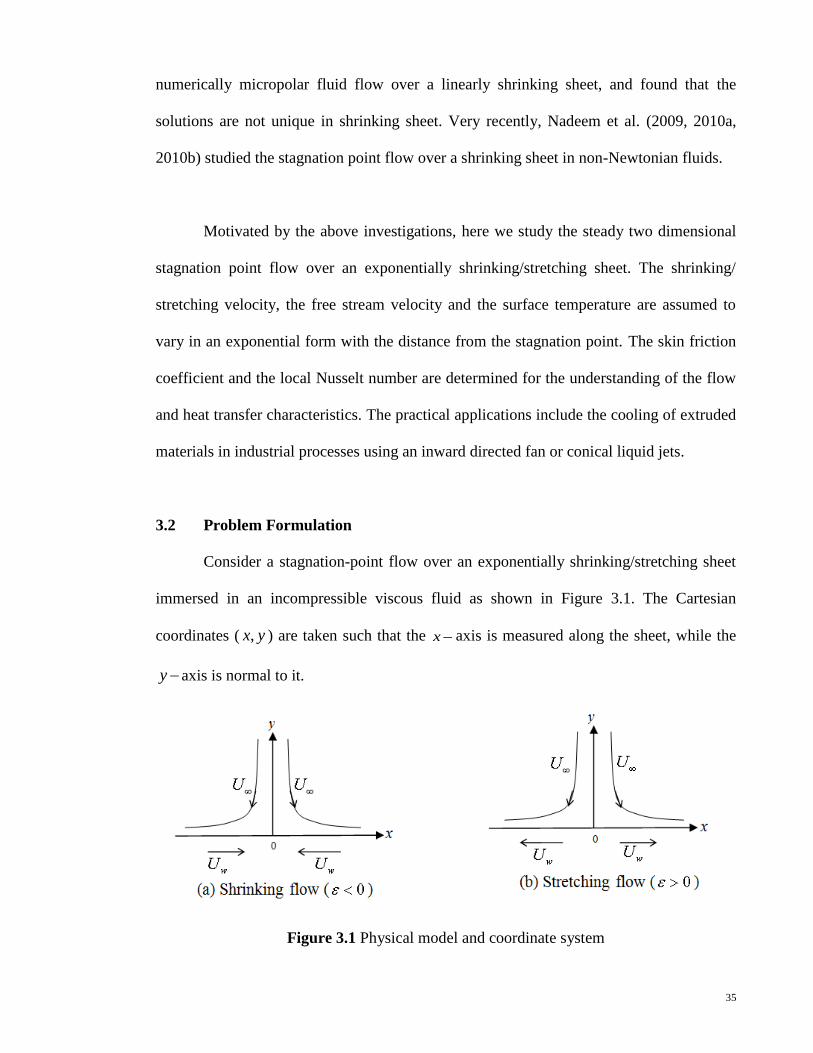
Consider a stagnation-point flow over an exponentially shrinking/stretching sheet

immersed in an incompressible viscous fluid as shown in Figure 3.1. The Cartesian

coordinates ( yx, ) are taken such that the x axis is measured along the sheet, while the

y axis is normal to it.

Figure 3.1 Physical model and coordinate system

36

It is assumed that the free stream velocity, the shrinking/stretching velocity and the

surface temperature are given by /x LU ae ,

/x L

wU be and /x L

wT T ce , respectively,

where a, b and c are constants and L is the reference length. The boundary layer equations

are (Magyari and Keller 1999; Ishak et al. 2009b; Bhattacharya & Layek 2011)

0u v

x y

, (3.1)

2

2

dUu u uu v U

x y dx y

, (3.2)

2

2

T T Tu v

x y y

, (3.3)

subject to the boundary conditions

wu U , 0v , wT T

at 0y ,

u U , T T as y , (3.4)

where vu and are the velocity components along the yx and axes, respectively,

is the thermal diffusivity of the fluid and is the kinematic viscosity.

Introducing the following similarity transformation (see Magyari & Keller 1999),

1/2

/(2 )

2

x Lae y

L

, / ( )x Lu ae f ,

1/2

/(2 )

2

x Lav e f f

L

,

37

( )w

T T

T T

, (3.5)

the continuity equation (3.1) is automatically satisfied, and Equations (3.2) and (3.3) are

reduced to

22 2 0f ff f , (3.6)

1

2 0Pr

f f , (3.7)

where primes denote differentiation with respect to and Pr / is the Prandtl number.

The transformed boundary conditions are

(0) 0f , (0)f , (0) 1 ,

( ) 1f , ( ) 0 as , (3.8)

with /b a being the shrinking/stretching parameter. We note that 0 is for

shrinking, 0 for stretching and 0 corresponds to a fixed sheet.

The main physical quantities of interest are the skin friction coefficient and the

local Nusselt number, which are proportional to the quantities (0)f and (0) ,

respectively. Thus, our aim is to investigate how the values of (0)f and (0) vary

with the shrinking or stretching parameter and the Prandtl number Pr.

38

3.3 Results and Discussion

Graphical results are presented for different physical parameters appearing in the

present model. We note that Equations (3.6) and (3.7) are decoupled, and thus the flow

field is not affected by the thermal field.

Figure 3.2 shows the variations of the skin friction coefficient (0)f against

shrinking/ stretching parameter , while the respective local Nusselt number (0) are

presented in Figure 3.3. Two branches of solutions are found to exist within the range

1c , while for 1 , the solution is unique. It is seen that for negative values of

(shrinking case), there is a critical value c where the upper branch meets the lower

branch. Based on our computation, 1.4872c . Beyond this critical value, no solution

exists. In these figures, the solid lines denote the upper branch, while the dash lines denote

the lower branch solutions. It is also evident from these figures that, the range of for

which the solution exists is very small for the shrinking case. This is due to the vorticity

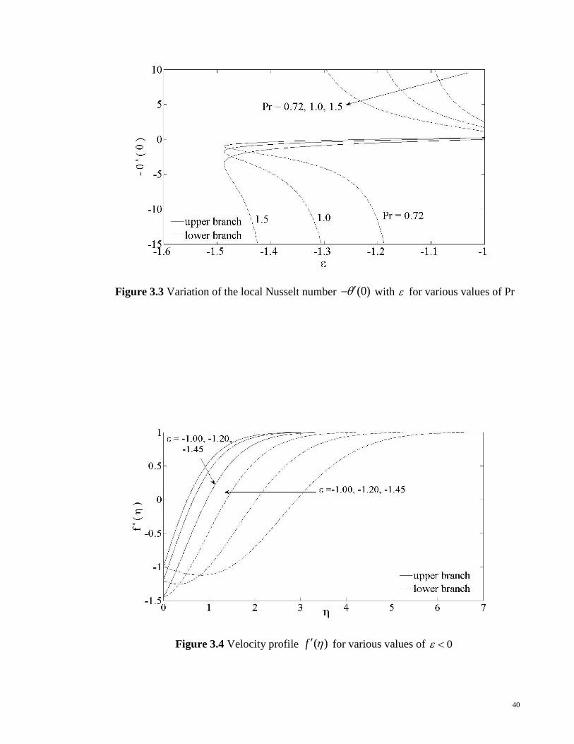
that almost cannot be confined in the boundary layer. It is observed in Figure 3.3 that the

lower branch solutions show discontinuity at -1.145, -1.255 and -1.375 for Pr= 0.72,

1.0 and 1.5 respectively. This phenomenon has been observed by other researchers in the

literature, for different problems, for example Ridha (1996) and Ishak et al. (2008d,

2010b). Further, it is found that when 1 (stretching case), the value of the skin friction

coefficient (0)f is zero. This is because when 1 , the stretching velocity is equal to

the external velocity, and thus there is no friction between the fluid and the solid surface.

Furthermore, when 1 , the exact solution of Equation (3.6) subject to the boundary

condition (3.8) can be obtained, and is given by ( )f , which then implies ( ) 0f

39

for all . The present numerical result agreed with this exact solution. It is also observed

that for the upper branch solution, (0) 0f when 1 and (0) 0f when 1 .

Physically, positive value of (0)f means the fluid exerts a drag force on the sheet, and

negative value means the opposite. On the other hand, the negative value of (0)f for the

lower branch solution as shown in Figure 3.2 is due to the back flow, see Figure 3.4. The

velocity gradient at the surface is negative for 1 and 1.2 , but is positive for

1.45 , which is in agreement with the results presented in Figure 3.2.

Figure 3.2 Variation of the skin friction coefficient (0)f with

40

Figure 3.3 Variation of the local Nusselt number (0) with for various values of Pr

Figure 3.4 Velocity profile ( )f for various values of 0

41

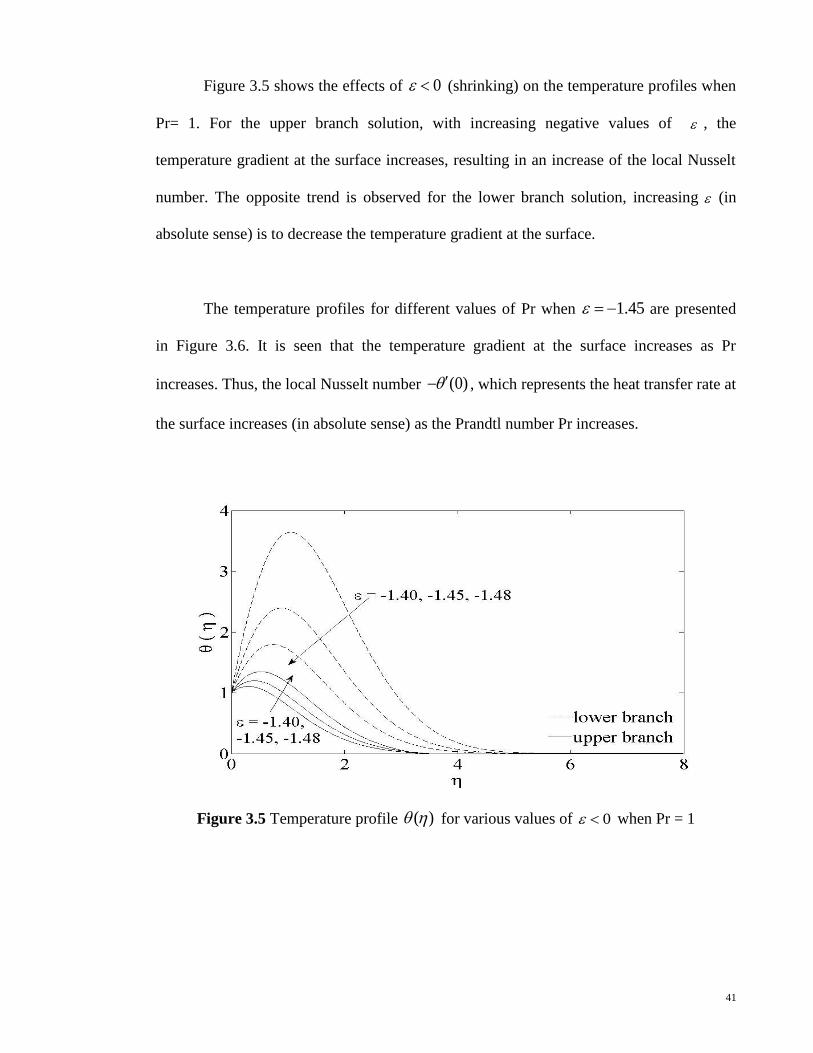
Figure 3.5 shows the effects of 0 (shrinking) on the temperature profiles when

Pr= 1. For the upper branch solution, with increasing negative values of , the

temperature gradient at the surface increases, resulting in an increase of the local Nusselt

number. The opposite trend is observed for the lower branch solution, increasing (in

absolute sense) is to decrease the temperature gradient at the surface.

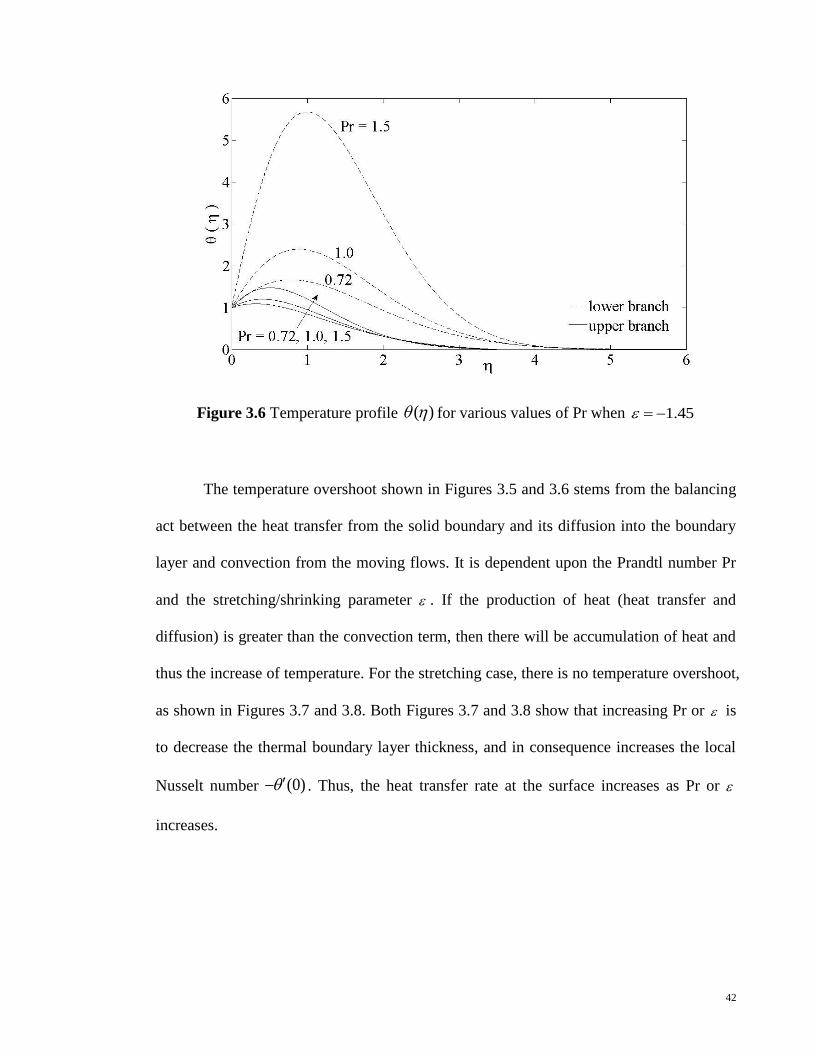
The temperature profiles for different values of Pr when 1.45 are presented

in Figure 3.6. It is seen that the temperature gradient at the surface increases as Pr

increases. Thus, the local Nusselt number (0) , which represents the heat transfer rate at

the surface increases (in absolute sense) as the Prandtl number Pr increases.

Figure 3.5 Temperature profile ( ) for various values of 0 when Pr = 1

42

Figure 3.6 Temperature profile ( ) for various values of Pr when 1.45

The temperature overshoot shown in Figures 3.5 and 3.6 stems from the balancing

act between the heat transfer from the solid boundary and its diffusion into the boundary

layer and convection from the moving flows. It is dependent upon the Prandtl number Pr

and the stretching/shrinking parameter . If the production of heat (heat transfer and

diffusion) is greater than the convection term, then there will be accumulation of heat and

thus the increase of temperature. For the stretching case, there is no temperature overshoot,

as shown in Figures 3.7 and 3.8. Both Figures 3.7 and 3.8 show that increasing Pr or is

to decrease the thermal boundary layer thickness, and in consequence increases the local

Nusselt number (0) . Thus, the heat transfer rate at the surface increases as Pr or

increases.

43

0 0.5 1 1.5 2 2.5 3 3.5 4-0.2

0

0.2

0.4

0.6

0.8

1

1.2

(

)Pr = 0.72, 1, 1.5

Figure 3.7 Temperature profile ( ) for various values of Pr when 0.5

Figure 3.8 Temperature profile ( ) for various values of when Pr = 1

44

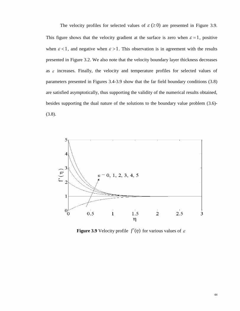
The velocity profiles for selected values of ( 0) are presented in Figure 3.9.

This figure shows that the velocity gradient at the surface is zero when 1 , positive

when 1 , and negative when 1 . This observation is in agreement with the results

presented in Figure 3.2. We also note that the velocity boundary layer thickness decreases

as increases. Finally, the velocity and temperature profiles for selected values of

parameters presented in Figures 3.4-3.9 show that the far field boundary conditions (3.8)

are satisfied asymptotically, thus supporting the validity of the numerical results obtained,

besides supporting the dual nature of the solutions to the boundary value problem (3.6)-

(3.8).

Figure 3.9 Velocity profile ( )f for various values of

45

3.4 Conclusions

The problem of stagnation-point flow over an exponentially shrinking/stretching

sheet immersed in an incompressible viscous fluid was investigated numerically.

Similarity solutions were obtained, and the effects of the governing parameters, namely

the shrinking/stretching parameter and the Prandtl number Pr on the fluid flow and heat

transfer characteristics were discussed. It was found that dual solutions exist for the

shrinking case, while for the stretching case, the solution is unique. Moreover, it was

found that increasing the Prandtl number is to increase the heat transfer rate at the surface.

46

CHAPTER 4

BOUNDARY LAYER FLOW AND HEAT TRANSFER OVER AN

EXPONENTIALLY STRETCHING/SHRINKING PERMEABLE SHEET WITH

VISCOUS DISSIPATION

4.1 Introduction

The study of fluid flow over a stretching/shrinking sheet has diverse technological

applications in industrial processes. Many of the industrial manufacturing processes

involve material sheeting production in metal or polymer sheet (Altan et al. 1983; Fisher

1976). For instance, manufacturing of glass fiber, drawing of plastic sheets, polymer melts,

metallic plate in a cooling bath, and the cooling and drying of papers. The quality of the

final products depends heavily on the rate of heat transfer at the stretching or shrinking

surface (Karwe & Jaluria 1988).

For these applications, Crane (1970) was one of the earlier pioneers to discuss two-

dimensional steady flow of an incompressible viscous fluid over a stretching sheet. He

gave a closed form solution for the boundary layer flow on a moving plate. Chen (1998)

analyzed the effect of thermal buoyancy forces on mixed convection boundary layer flow

pass a stretching sheet, where the temperature varies in a power law form. He reported that

the buoyancy force parameter induced the surface heat transfer rate. Similar fluid flows

induced by stretching sheet have been considered by several researchers in various aspects

(see Ishak et al. 2006b, 2007; Ishak 2009; Bataller 2008a, 2008b; Weidman & Ali 2011).

47

Besides the flow due to a stretching sheet as discussed, our objective is also to

discuss the flow and heat transfer characteristics that are brought about by the shrinking

sheet. This type of flows has been considered by several authors. One of the earlier fluid

flows of this nature was first discussed by Miklavčič and Wang (2006). Their numerical

solution becomes non-unique after some critical mass suction s . For stretching sheet,

previous studies (Gupta & Gupta 1977) show that the solutions are unique for all suction

rates. Later, Wang (2008) studied the effects of axisymmetric stagnation point flow over a

shrinking/stretching sheet in power-law form. The axisymmetric case shows that for

shrinking with suction rate 1.2465s , no solution exists.

However, there are other various interesting studies in stretching or shrinking cases.

Van Gorder and Vajravelu (2011) studied second grade fluid flows over an exponentially

stretching or shrinking surface which admits an explicit exact solution. Van Gorder (2010)

also investigated the nonlinear boundary value problems inclusive of mass transfer with

exponentially decaying solution and provided the criterion for the existence of single and

multiple solutions. Fang and Zhang (2009) obtained exact solution for MHD flow over a

linear shrinking sheet with suction and injection. Multiple solution branches were

observed for certain mass suction parameter. Later, Fang et al. (2009) considered unsteady

flow through shrinking sheet in porous medium. They showed that for mass suction 2s ,

the solution exists. Recently, researchers such as Cortell (2010), Noor et al. (2010), Fang

et al. (2010), Merkin and Kumaran (2010) and Ishak et al. (2010a) have numerically

studied the flow induced by a shrinking sheet with diversely different features, for

example micropolar fluid, unsteady state, MHD and second order slip flows.

48

Motivated by the above investigations, we study the boundary layer flow and heat

transfer over an exponentially stretching/shrinking permeable sheet with viscous

dissipation. The skin friction coefficient and the local Nusselt number are determined for

the flow field and the thermal field, respectively.

4.2 Problem Formulation

Consider a steady two-dimensional boundary layer flow and heat transfer of a

viscous and incompressible fluid over an exponentially stretching/shrinking permeable

sheet as shown in Figure 4.1. The Cartesian coordinates ( yx, ) are taken such that the

x axis is measured along the sheet oriented in the horizontal direction and the y axis is

perpendicular to it.

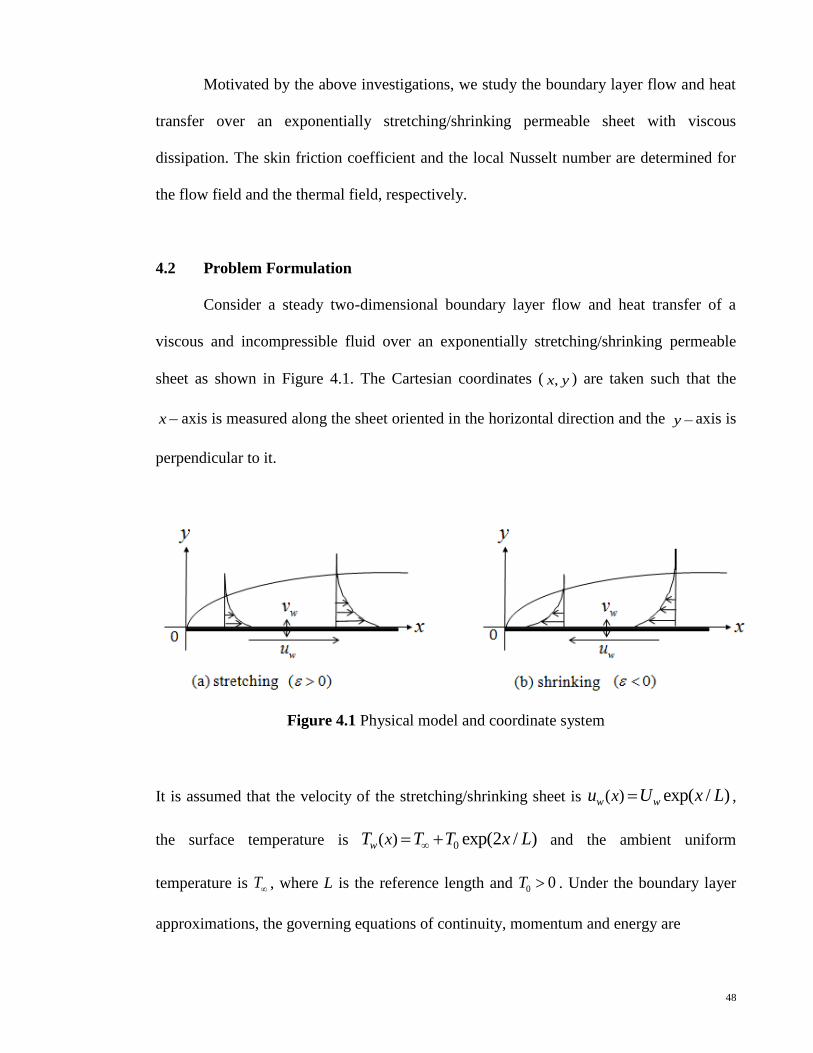
Figure 4.1 Physical model and coordinate system

It is assumed that the velocity of the stretching/shrinking sheet is ( ) exp( / )w wxu U x L ,

the surface temperature is 0( ) exp(2 / )w xT T T x L and the ambient uniform

temperature is T , where L is the reference length and 0 0T . Under the boundary layer

approximations, the governing equations of continuity, momentum and energy are

49

0u v

x y

, (4.1)

2

2

u u uu v

x y y

, (4.2)

22

2p

T T T uC u v k

x y y y

, (4.3)

subject to the boundary conditions

( )wu u x , ( )wv v x , ( )wT T x at 0y ,

0u , T T as y , (4.4)

where + and – signs correspond to a stretching and a shrinking sheet, respectively, is the

kinematic viscosity, the fluid density, pC the specific heat at constant pressure, k the

thermal conductivity and is the dynamic viscosity.

To obtain similarity solution, we introduce the following similarity variables:

,2

exp2

),/()()(),(2

exp2

L

x

L

Uy

TTTTfL

xUL

w

ww

(4.5)

where is the stream function defined as /u y and /v x , which identically

satisfies Equation (4.1). By this definition, we obtain

50

exp ( ), exp ( ) ( )2 2

ww

Ux xu U f v f f

L L L

(4.6)

where prime denotes differentiation with respect to . Further, to obtain similarity

solution, we take

( ) exp2 2

ww

U xv x s

L L

(4.7)

where (0)s f is a constant: 0s corresponds to suction, 0s corresponds to injection

or blowing , 0s corresponds to an impermeable surface.

Substituting (4.5) and (4.6) into Equations (4.2) and (4.3), we obtain the following

system of nonlinear ordinary differential equations:

22 0f ff f , (4.8)

214 Ec 0

Prf f f . (4.9)

The boundary conditions (4.4) then become

(0)f s , (0)f , (0) 1 ,

( ) 0f , ( ) 0 as , (4.10)

51

where 1 is the stretching/shrinking parameter, Pr is the Prandtl number and Ec is

the Eckert number, which are defined as

2

0

Pr , Ec .p w

p

C U

k T C

(4.11)

Here 1 denotes stretching sheet whilst 1 is a shrinking sheet.

The main physical characteristics of interest in the present problem are the skin

friction coefficient fC and the local Nusselt number xNu , which are defined as

2

, ( )

w wf x

w w

xqC Nu

u k T T

, (4.12)

respectively, where the surface shear stress w and the surface heat flux wq are given by

0 0

, .w w

y y

u Tq k

y y

(4.13)

Substituting (4.5) into Equations (4.12) give

1 1

2 21/2 1/22 2

Re (0) , Re (0)f x x x

L LC f Nu

x x

(4.14)

where Re /x wu x is the local Reynolds number.

52

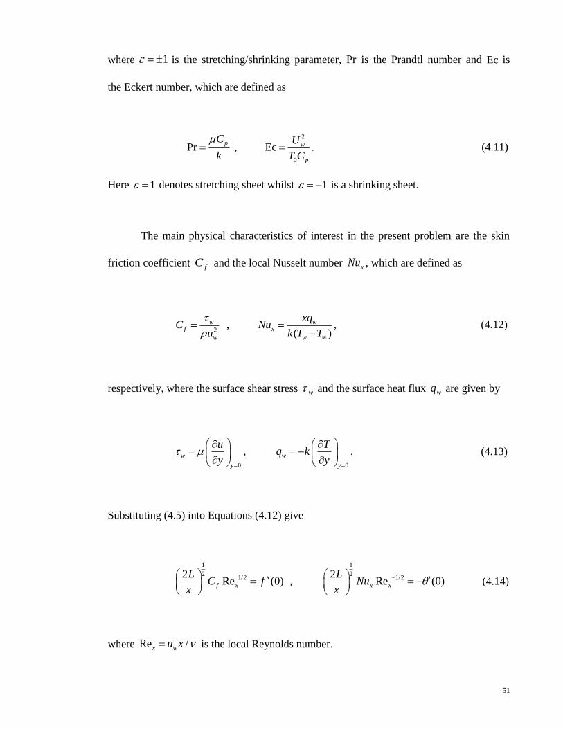
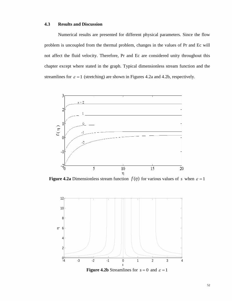
4.3 Results and Discussion

Numerical results are presented for different physical parameters. Since the flow

problem is uncoupled from the thermal problem, changes in the values of Pr and Ec will

not affect the fluid velocity. Therefore, Pr and Ec are considered unity throughout this

chapter except where stated in the graph. Typical dimensionless stream function and the

streamlines for 1 (stretching) are shown in Figures 4.2a and 4.2b, respectively.

Figure 4.2a Dimensionless stream function ( )f for various values of s when 1

Figure 4.2b Streamlines for 0s and 1

-4 -3 -2 -1 0 1 2 3 40

2

4

6

8

10

12

x

53

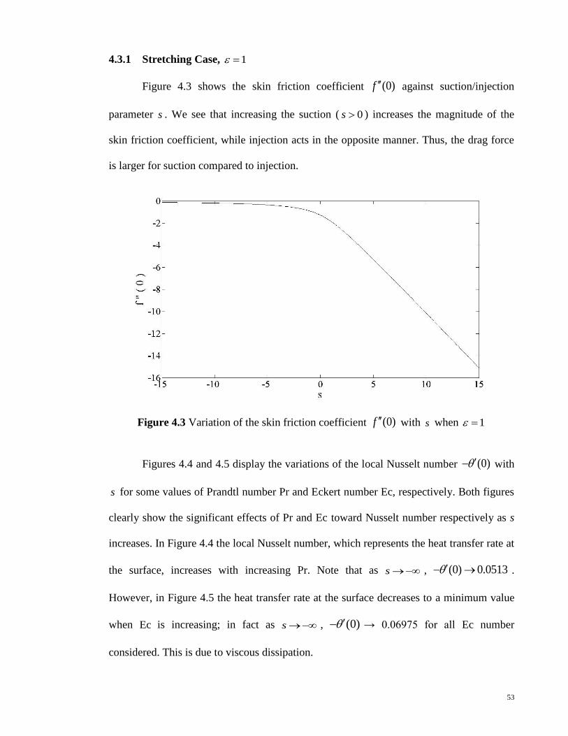
4.3.1 Stretching Case, 1

Figure 4.3 shows the skin friction coefficient (0)f against suction/injection

parameter s . We see that increasing the suction ( 0s ) increases the magnitude of the

skin friction coefficient, while injection acts in the opposite manner. Thus, the drag force

is larger for suction compared to injection.

Figure 4.3 Variation of the skin friction coefficient (0)f with s when 1

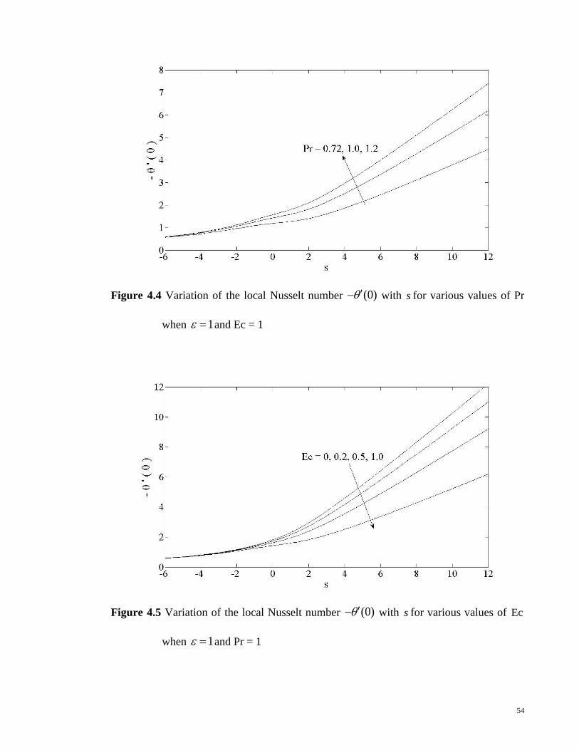
Figures 4.4 and 4.5 display the variations of the local Nusselt number (0) with

s for some values of Prandtl number Pr and Eckert number Ec, respectively. Both figures

clearly show the significant effects of Pr and Ec toward Nusselt number respectively as s

increases. In Figure 4.4 the local Nusselt number, which represents the heat transfer rate at

the surface, increases with increasing Pr. Note that as s , (0) 0.0513 .

However, in Figure 4.5 the heat transfer rate at the surface decreases to a minimum value

when Ec is increasing; in fact as s , (0) → 0.06975 for all Ec number

considered. This is due to viscous dissipation.

54

Figure 4.4 Variation of the local Nusselt number (0) with s for various values of Pr

when 1 and Ec = 1

Figure 4.5 Variation of the local Nusselt number (0) with s for various values of Ec

when 1 and Pr = 1

55

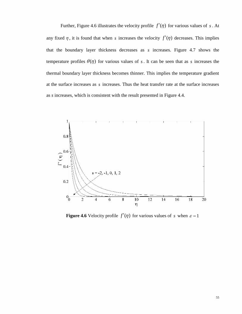
Further, Figure 4.6 illustrates the velocity profile ( )f for various values of s . At

any fixed , it is found that when s increases the velocity ( )f decreases. This implies

that the boundary layer thickness decreases as s increases. Figure 4.7 shows the

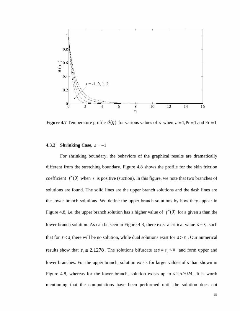
temperature profiles ( ) for various values of s . It can be seen that as s increases the

thermal boundary layer thickness becomes thinner. This implies the temperature gradient

at the surface increases as s increases. Thus the heat transfer rate at the surface increases

as s increases, which is consistent with the result presented in Figure 4.4.

Figure 4.6 Velocity profile ( )f for various values of s when 1

56

Figure 4.7 Temperature profile ( ) for various values of s when 1,Pr 1 and Ec 1

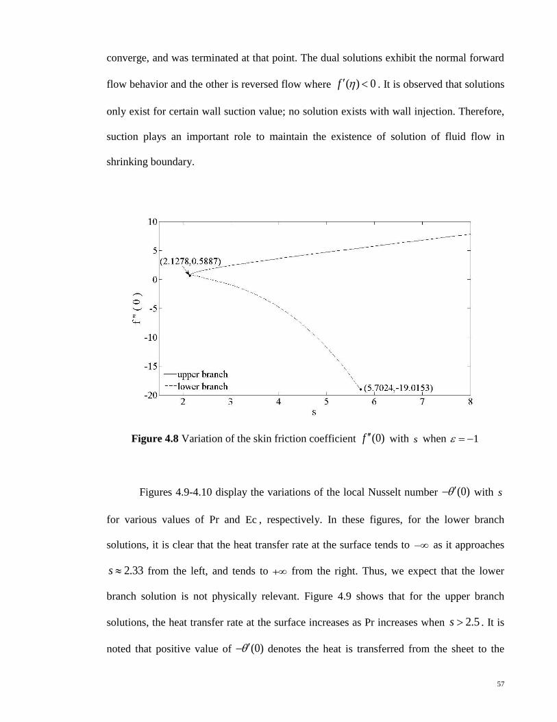
4.3.2 Shrinking Case, 1

For shrinking boundary, the behaviors of the graphical results are dramatically

different from the stretching boundary. Figure 4.8 shows the profile for the skin friction

coefficient (0)f when s is positive (suction). In this figure, we note that two branches of

solutions are found. The solid lines are the upper branch solutions and the dash lines are

the lower branch solutions. We define the upper branch solutions by how they appear in

Figure 4.8, i.e. the upper branch solution has a higher value of (0)f for a given s than the

lower branch solution. As can be seen in Figure 4.8, there exist a critical value cs s such

that for cs s there will be no solution, while dual solutions exist for cs s . Our numerical

results show that 2.1278cs . The solutions bifurcate at 0c

s s and form upper and

lower branches. For the upper branch, solution exists for larger values of s than shown in

Figure 4.8, whereas for the lower branch, solution exists up to 5.7024s . It is worth

mentioning that the computations have been performed until the solution does not

57

converge, and was terminated at that point. The dual solutions exhibit the normal forward

flow behavior and the other is reversed flow where ( ) 0f . It is observed that solutions

only exist for certain wall suction value; no solution exists with wall injection. Therefore,

suction plays an important role to maintain the existence of solution of fluid flow in

shrinking boundary.

Figure 4.8 Variation of the skin friction coefficient (0)f with s when 1

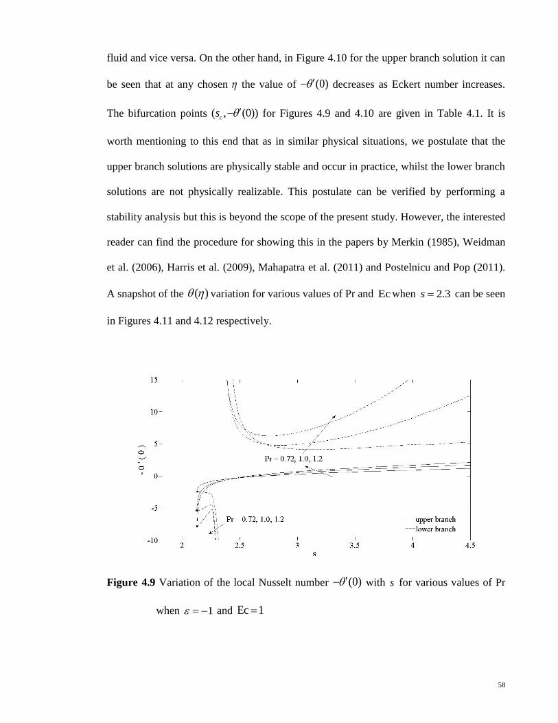
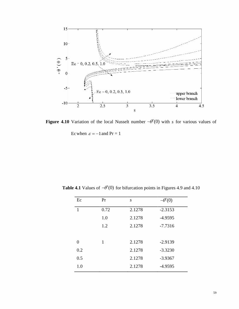
Figures 4.9-4.10 display the variations of the local Nusselt number (0) with s

for various values of Pr and Ec , respectively. In these figures, for the lower branch

solutions, it is clear that the heat transfer rate at the surface tends to as it approaches

2.33s from the left, and tends to from the right. Thus, we expect that the lower

branch solution is not physically relevant. Figure 4.9 shows that for the upper branch

solutions, the heat transfer rate at the surface increases as Pr increases when 2.5s . It is

noted that positive value of (0) denotes the heat is transferred from the sheet to the

58

fluid and vice versa. On the other hand, in Figure 4.10 for the upper branch solution it can

be seen that at any chosen the value of (0) decreases as Eckert number increases.

The bifurcation points ( , (0))cs for Figures 4.9 and 4.10 are given in Table 4.1. It is

worth mentioning to this end that as in similar physical situations, we postulate that the

upper branch solutions are physically stable and occur in practice, whilst the lower branch

solutions are not physically realizable. This postulate can be verified by performing a

stability analysis but this is beyond the scope of the present study. However, the interested

reader can find the procedure for showing this in the papers by Merkin (1985), Weidman

et al. (2006), Harris et al. (2009), Mahapatra et al. (2011) and Postelnicu and Pop (2011).

A snapshot of the ( ) variation for various values of Pr and Ecwhen 2.3s can be seen

in Figures 4.11 and 4.12 respectively.

Figure 4.9 Variation of the local Nusselt number (0) with s for various values of Pr

when 1 and Ec 1

59

Figure 4.10 Variation of the local Nusselt number (0) with s for various values of

Ecwhen 1 and Pr = 1

Table 4.1 Values of (0) for bifurcation points in Figures 4.9 and 4.10

Ec Pr s (0)

1 0.72 2.1278 -2.3153

1.0 2.1278 -4.9595

1.2 2.1278 -7.7316

0 1 2.1278 -2.9139

0.2 2.1278 -3.3230

0.5 2.1278 -3.9367

1.0 2.1278 -4.9595

60

Figure 4.11 Temperature ( ) variation, with 2.3s and Ec 1 , for various values of

Pr when 1 .

Figure 4.12 Temperature ( ) variation, with 2.3s and Pr 1 , for various values of

Ec when 1 .

61

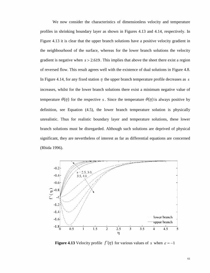
We now consider the characteristics of dimensionless velocity and temperature

profiles in shrinking boundary layer as shown in Figures 4.13 and 4.14, respectively. In

Figure 4.13 it is clear that the upper branch solutions have a positive velocity gradient in

the neighbourhood of the surface, whereas for the lower branch solutions the velocity

gradient is negative when 2.619s . This implies that above the sheet there exist a region

of reversed flow. This result agrees well with the existence of dual solutions in Figure 4.8.

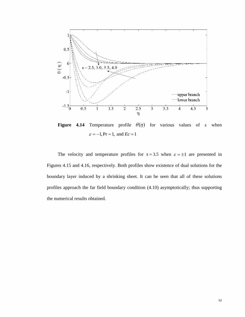
In Figure 4.14, for any fixed station the upper branch temperature profile decreases as s

increases, whilst for the lower branch solutions there exist a minimum negative value of

temperature ( ) for the respective s . Since the temperature ( ) is always positive by

definition, see Equation (4.5), the lower branch temperature solution is physically

unrealistic. Thus for realistic boundary layer and temperature solutions, these lower

branch solutions must be disregarded. Although such solutions are deprived of physical

significant, they are nevertheless of interest as far as differential equations are concerned

(Rhida 1996).

Figure 4.13 Velocity profile ( )f for various values of s when 1

62

Figure 4.14 Temperature profile ( ) for various values of s when

1,Pr 1, and 1Ec

The velocity and temperature profiles for 3.5s when 1 are presented in

Figures 4.15 and 4.16, respectively. Both profiles show existence of dual solutions for the

boundary layer induced by a shrinking sheet. It can be seen that all of these solutions

profiles approach the far field boundary condition (4.10) asymptotically; thus supporting

the numerical results obtained.

63

Figure 4.15 Velocity profile ( )f when 3.5s for 1

Figure 4.16 Temperature profile ( ) for 1 when 3.5,Pr 1, 1s Ec

64

4.4 Conclusions

The problem of boundary layer flow and heat transfer over an exponentially

stretching/shrinking permeable sheet with viscous dissipation was investigated

numerically. Similarity equations were obtained and solved numerically, and the effects of

the governing parameters on the fluid flow and heat transfer characteristics were

discussed. It was found that dual solutions exist for the shrinking boundary, while for the

stretching boundary, the solution is always unique. Moreover, it was found that suction

increases both the skin friction coefficient and the heat transfer rate at the surface.

65

CHAPTER 5

CONCLUSIONS AND FUTURE WORK

In this thesis, we have studied the viscous fluid flows and heat transfer boundary

layer problems over a stretching or shrinking sheet. We have derived the general equations

for fluid motion and heat transfer from the laws of conservation of mass, linear and

angular momentum and energy in Chapter 1. Under the assumption of Prandtl’s boundary

layer theory and order of magnitude analysis, as well as focusing on steady state and two

dimensional problems, the set of nonlinear PDE Navier-Stokes equations are reduced to

steady, two-dimensional incompressible boundary layer fluid flows and heat transfer

equations. Later, we have made use of the similarity transformation to reduce the

governing boundary layer partial differential equations to a system of nonlinear ordinary

differential equations. Therefore these resulting nonlinear systems of ODEs are now

amenable to be solved numerically. In this thesis our objective is to study flows and heat

transfer rates in the vicinity of stagnation point. At this point the flow velocity is at its

minimum whilst the heat transfer rate is at its maximum.

We used the Keller-box method, originally suggested by Keller (1970), to solve

the reduced governing nonlinear ordinary differential equations. The method is second

order and unconditionally stable. Central differences techniques are constructed to replace

the derivatives and the resulting non-linear difference equations are linearised by

Newton’s method. Then the linearised equations are solved by the block tridiagonal

elimination method. The Keller box method has been applied to the three different

problems respectively in Chapter 2-4.

66

In Chapter 2, we studied the effect of buoyancy forces towards a stretching vertical

sheet immersed in viscous fluid, with the sheet velocity given in power form. The far field

velocity is also of the power form. The buoyancy forces are either of assisting or opposing

the fluid motion in the boundary layer. From our calculations, for assisting buoyancy force,

all solutions are unique. In the case of opposing buoyancy force, dual solutions are

obtained up to a certain critical value c . This critical value c depends on the values of

velocity exponent parameter m and the velocity ratio parameter . The higher the velocity

exponent parameter m , the higher is this critical value c . The value of c also increases

when the velocity ratio parameter increases.

In Chapter 3, we discussed the stagnation point flow over a stretching or shrinking

sheet immersed in viscous fluid, with the sheet in the horizontal direction. The deduced

boundary layer equations are decoupled. The sheet velocity, far field fluid velocity and

surface temperature are given in exponential form. The stretching or shrinking parameter

is given by , with 0 denoting stretching and 0 shrinking. Our results show that

all solutions are unique for 1 , that is for all stretching and shrinking cases. For the

shrinking case, dual solutions are obtained from 1 up to a critical value

1.4872c . This agrees very well with the results of Bhattacharyya and Vajravelu

(2011). For heat transfer rate our results show that for stretching rate 1 , the heat

transfer rate increases as Prandtl Pr increases. This is also true for any other 0 . When

1 , the exact solution for the fluid velocity field is ( )f .

67

In Chapter 4, the above problem in Chapter 3 is extended to include the effects of

mass transfer and viscous dissipation. The suction or injection parameter is given by s,

with 0s denoting suction and 0s injection. From our calculation, for the stretching

case, all solutions are unique for either suction or injection. However, in the shrinking case,

dual solutions are obtained from 5.7024s down to a critical value 2.1278cs . No

solution exists smaller than this critical value cs , that is no solution exists for cs s for

injection case. This agrees very well with the results of Bhattacharyya (2011). For heat

transfer rate, our calculations show that for stretching case, the heat transfer rate increases

as Prandtl Pr increases. Whilst the heat transfer rate increases when Eckert Ec decreases.

Looking ahead, in this thesis we have successfully analyzed exponentially form

forced convection boundary layer problem in Chapter 3 and also a similar problem in

Chapter 4 but with mass transfer through the sheet. We can extend this idea of exponential

form to the body temperature or temperature heat flux and then letting the created motion

to settle down. This is free convection. But most problems of this nature are mixed

convection. Thus free and mixed convection studies can be made in future investigation.

The effects of magnetic field, porous medium, heat flux, slip condition, non-Newtonian

fluids such as micropolar fluids can also be considered. However the current algorithms

developed for solving the system of nonlinear ODEs in this study are second order

accurate and the accuracy is found wanting. Apart from that, a systematics method not

only to relate and computational accuracy but also searching multisolutions and higher

convergence should be looked into seriously. Therefore, a higher order accuracy algorithm

and a more robust and stable scheme is needed to study these more delicate free and

mixed convection problems.

68

REFERENCES

Acheson, D. J. (1990). Elementary fluid dynamics. New York: Oxford University Press

Inc.

Ali, F. M., Nazar, R., Arifin, N. M., & Pop, I. (2011). Unsteady shrinking sheet with mass

transfer in a rotating fluid. International Journal for Numerical Methods in Fluids

66:1465–1474.

Altan, T., Oh, S. I., & Gegel, H. L. (1983). Metal forming fundamentals and applications.

American Society for Metals, Metal Park, Ohio.

Andersson, H. I., Back, K. H., & Dandapat, B. S. (1992). Magnetohydrodynamic flow of a

power-law fluid over a stretching sheet. International Journal of Non-Linear

Mechanics 27: 929-939.

Bataller, R. C. (2008a). Radiation effects in the Blasius flow. Applied Mathematics and

Computation 198:333-338.

Bataller, R. C. (2008b). Similarity solution for flow and heat transfer of a quiescent fluid

over a nonlinearly stretching surface. Journal of Materials Processing Technology

203:176-183.

Bhattacharyya, K. (2011). Boundary layer flow and heat transfer over an exponentially

shrinking sheet. Chinese Physics Letters28:074701/

Bhattacharyya, K., & Layek, G. C. (2011). Effects of suction/blowing on steady boundary

layer stagnation-point flow and heat transfer towards a shrinking sheet with thermal

radiation. International Journal of Heat and Mass Transfer 54:302-307.

Bhattacharyya, K., & Vajravelu, K. (2011). Stagnation-point flow and heat transfer over

an exponentially shrinking sheet. Communications in Nonlinear Sciences and

Numerical Simulation 17:2728-2734.

69

Bidin, B. & Nazar, R. (2009). Numerical solution of the boundary layer flow over an

exponentially stretching sheet with thermal radiation. European Journal of Scientific

Research 33:710 – 717.

Chen, C. H. (1998). Laminar mixed convection adjacent to vertical, continuously

stretching sheets. Heat Mass Transfer 33:471-476.

Cortell, R. (2010). On a certain boundary value problem arising in shrinking sheet flows.

Applied Mathematics and Computation 217:4086-4093.

Crane, L. J. (1970). Flow past a stretching plane. Journal of Applied Mathematics and

Physics (ZAMP) 21:645-647.

Daily, J. W., & Harleman D. R. F. (1966). Fluid Dynamics. Reading, MA: Addison-

Wesley, 1966.

El-Aziz, M. A. (2009). Viscous dissipation effect on mixed convection flow of a

micropolar fluid over an exponentially stretching sheet. Canadian Journal of Physics

87:359-368.

Fang, T. (2008). Boundary layer flow over a shrinking sheet with power-law velocity.

International Journal of Heat and Mass Transfer 51:5838-5843.

Fang, T., Yao, S., Zhang, J., & Aziz, A. (2010). Viscous flow over a shrinking sheet with

a second order slip flow model. Communications in Nonlinear Science and

Numerical Simulation 15:1831-1842.

Fang, T., & Zhang, J. (2009). Closed-form exact solution of MHD viscous flow over a

shrinking sheet. Communications in Nonlinear Science and Numerical Simulation

14:2853-2857.

Fang, T., Zhang, J., & Yoa, S. (2009). Viscous flow over an unsteady shrinking sheet with

mass transfer. Chinese Physics Letters 26:014703.

Fisher E.G. (1976). Extrusion of Plastics. Wiley: New York.

70

Fourier, J. B. (1822). Theorie Analytique de la Chaleur. Didot, Paris.

Gupta, P. S., & Gupta, A. S. (1977). Heat and mass transfer on a stretching sheet with

suction or blowing. The Canadian Journal of Chemical Engineering 55:744-746.

Harris, S. D., Ingham, D. B., & Pop, I. (2009). Mixed convection boundary-layer flow

near the stagnation point on a vertical surface in a porous medium: Brinkman model

with slip. Transport in Porous Media 77:267–285.

Hossain, M. A., & Takhar, H. S. (1996). Radiation effect on mixed convection along a

vertical plate with uniform surface temperature. Heat Mass Transfer 31:243-248.

Ishak, A., Nazar, R., & Pop, I. (2006a). Unsteady mixed convection boundary layer flow

due to a stretching vertical surface. Arabian Journal for Science and Engineering

31:165-182.

Ishak, A., Nazar, R., & Pop, I. (2006b). Unsteady mixed convection boundary layer flow

due to a stretching vertical surface. The Arabian Journal for Science and

Engineering 31: 165 – 181.

Ishak, A., Nazar, R., & Pop, I. (2007). Boundary layer flow of a micropolar fluid on a

continuously moving or fixed permeable surface. International Journal of Heat and

Mass Transfer 50:4743-4748.

Ishak, A., Nazar, R., Pop, I. (2008a). Post-stagnation point boundary layer flow and mixed

convection heat transfer over a vertical, linearly stretching sheet. Archives of

Mechanics 60 (4): 303-322.

Ishak, A., Nazar, R., Pop, I. (2008b). Mixed convection stagnation point flow of a

micropolar fluid towards a stretching sheet. Meccanica 43:411-418.

Ishak, A., Nazar, R., Pop, I. (2008c). Hydromagnetic flow and heat transfer adjacent to a

stretching vertical sheet. Journal of Heat Mass Transfer 44: 921-927.

71

Ishak, A., Nazar, R., Arifin, N. M., & Pop, I. (2008d). Dual solutions in mixed convection

flow near a stagnation point on a vertical porous plate. International Journal of

Thermal Sciences 47:417-422.

Ishak, A. (2009). Radiation effects on the flow and heat transfer over a moving plate in a

parallel stream. Chinese Physics Letters 26: 034701.

Ishak, A., Nazar, R., Pop, I. (2009a). Boundary layer flow and heat transfer over an

unsteady stretching vertical surface. Meccanica 44: 369-375.

Ishak, A., Jafar, K., Nazar, R., & Pop, I. (2009b). MHD stagnation point flow towards a

stretching sheet. Physica A: Statistical Mechanics and its Applications 388:3377-

3383.

Ishak, A., Lok, Y. Y., & Pop, I. (2010a). Stagnation-point flow over a shrinking sheet in a

micropolar fluid. Chemical Engineering Communications 197: 1417–1427.

Ishak, A., Nazar, R., Bachok, N., & Pop, I. (2010b). MHD mixed convection flow

adjacent to a vertical plate with prescribed surface temperature. International

Journal of Heat and Mass Transfer 53:4506-4510.

Ishak, A. (2011). MHD boundary layer flow due to an exponentially stretching sheet with

radiation effect. Sains Malaysiana 40:391-395.

Karwe, M. V., & Jaluria, Y. (1988). Fluid flow and mixed convection transport from a

moving plate in rolling and extrusion processes. ASME Journal of Heat Mass

Transfer 110:655-661.

Karwe, M. V., & Jaluria, Y. (1991). Numerical simulation of thermal transport associated

with a continuously moving flat sheet in materials processing. ASME Journal of

Heat Transfer 113:612-619.

72

Keller, H. B. (1970). A new difference scheme for parabolic problems, in: J. Bramble 341

(Ed.), Numerical Solution of Partial-Differential Equations, vol. II. Academic, New

York.

Keller, H. B. & Cebeci, T. (1971). Accurate numerical methods for boundary layer flows,

I: Two-dimensional laminar flow. Proceeding of the 2nd

International Conference on

Numerical solutions of partial differential equations. New York: Springer-Verlag.

Keller, H. B. & Cebeci, T. (1972). Accurate numerical methods for boundary layer flows,

II: Two-dimensional turbulent flows. AIAA Journal 10: 1193-1199.

Kestin, J. (1966). A course in Thermodynamics. Vol. II, Blaisdell.

Magyari, E. & Keller, B. (1999). Heat and mass transfer in the boundary layers on an

exponentially stretching continuous surface. Journal of Physics D: Applied Physics

32: 577–585.

Mahapatra, T. R., Nandy, S. K., Vajravelu, K., & Van Gorder, R. A. (2011). Stability

analysis of fluid flow over a nonlinearly stretching sheet. Archive Applied Mechanics

81:1087-1091.

Merkin, J. H., & Mahmood, T. (1989). Mixed convection boundary layer similarity

solutions: prescribed wall heat flux. Journal of Applied Mathematics and Physics

40:51–68.

Merkin, J. H., & Kumaran, V. (2010). The unsteady MHD boundary layer flow on a

shrinking sheet. European Journal of Mechanics B/Fluids 29:357-363.

Merkin, J. H. (1985). On dual solutions occurring in mixed convection in a porous

medium. Journal of Engineering Mathematics 20:171–179.

Miklavčič, M. & Wang, C. Y. (2006). Viscous flow due to a shrinking sheet. Quarterly of

Applied Mathematics 64:283–290.

73

Nadeem, S., & Awais, M. (2008). Thin film flow of an unsteady shrinking sheet through

porous medium with variable viscosity. Physics Letters A 372:4965-4972.

Nadeem, S., Abbasbandy, S., & Hussain, M. (2009). Series solutions of boundary layer

flow of a micropolar fluid near the stagnation point towards a shrinking sheet.

Zeitschrift fur Naturforschung A 64:575- 582.

Nadeem, S., Hussain, A., & Vajravelu, K. (2010a). Effects of heat transfer on the

stagnation flow of a third-order fluid over a shrinking sheet. Zeitschrift fur

Naturforschung A 65:969-994.

Nadeem, S., Hussain, A., & Khan, M. (2010b). Stagnation flow of a Jeffrey fluid over a

shrinking sheet. Zeitschrift fur Naturforschung A 65:540-548.

Nazar, R., Amin, N., Flip, D., & Pop, I. (2004). Unsteady boundary layer flow in the

region of the stagnation point on a stretching sheet. International Journal of

Engineering Science 42:1241-1253.

Noor, N. F. M., Kechil, S. A., & Hashim, I. (2010). Simple non-perturbative solution for

MHD viscous flow due to a shrinking sheet. Communications in Nonlinear Science

and Numerical Simulation 15:144-148.

Pal, D. (2010). Mixed convection heat transfer in the boundary layers on an exponentially

stretching surface with magnetic field. Applied Mathematics and Computation

217:2356-2369.

Postelnicu, A., & Pop, I. (2011). Falkner-Skan boundary layer flow of a power-law fluid

past a stretching wedge. Applied Mathematics and Computation 217:4359–4368.

Ramachandran, N., Chen, T. S., & Armaly, B. F. (1988). Mixed convection in stagnation

flows adjacent to vertical surfaces. ASME Journal of Heat Mass Transfer 110: 373–

377.

74

Ridha, A. (1996). Aiding flows non-unique similarity solutions of mixed convection

boundary layer equations. Journal of Applied Mathematics and Physics (ZAMP)

47:341-352.

Saha, L. K., Hossain, M. A., & Gorla, R. S. R. (2007). Effect of Hall current on the MHD

laminar natural convection flow from a vertical permeable flat plate with uniform

surface temperature. International Journal of Thermal Sciences 46: 790–801.

Sajid, M. & Hayat, T. (2008). Influence of thermal radiation on the boundary layer flow

due to an exponentially stretching sheet. International Communications in Heat and

Mass Transfer 35: 347–356.

Sajid, M., Javed, T., & Hayat, T. (2008). MHD rotating flow of a viscous fluid over a

shrinking surface. Nonlinear Dynamics 51:259-265.

Sanjayanand, E. & Khan, S. K. (2006). On heat and mass transfer in a viscoelastic

boundary layer flow over an exponentially stretching sheet. International Journal of

Thermal Sciences 45:819-828.

Schlichting, H. (1979). Boundary-Layer Theory, 7th

ed. New York: McGraw-Hill.

Van Gorder, R. A. (2010). High-order nonlinear boundary value problems admitting

multiple exact solutions with application to the fluid flow over a sheet. Applied

Mathematics and Computation 216:2177-2182.

Van Gorder, R. A., & Vajravelu, K. (2011). Multiple solutions for hydromagnetic flow of

a second grade fluid over a stretching or shrinking sheet. Quarterly of Applied

Mathematics 69:405-424.

Wang, C. Y. (2008). Stagnation flow towards a shrinking sheet. International Journal of

Non-linear Mechanics 43: 377–382.

75

Weidman, P. D., Kubitschek, D. G., & Davis, A. M. J. (2006). The effect of transpiration

on self-similar boundary layer flow over moving surface. International Journal of

Engineering Science 44:730–737.

Weidman, P. D., & Ali, M. E. (2011). Aligned and nonaligned radial stagnation flow on a

stretching cylinder. European Journal of Mechanics B/Fluids 30:120-128.

White, F. M. (2000) Viscous Fluid Flow, 3rd

ed. New York: McGraw-Hill.

Yih, K. A. (1998). Coupled heat and mass transfer in mixed convection over a vertical flat

plate embedded in saturated porous media: PST/PSC or PHF/PMF. Heat and Mass

Transfer 34: 55-61.