Working Paper 21-047

The Stock Market Valuation of Human Capital Creation

Matthias Regier Ethan Rouen

Working Paper 21-047

Copyright © 2020, 2021, 2022 by Matthias Regier and Ethan Rouen.

Working papers are in draft form. This working paper is distributed for purposes of comment and discussion only. It may not be reproduced without permission of the copyright holder. Copies of working papers are available from the author.

Funding for this research was provided in part by Harvard Business School.

The Stock Market Valuation of Human Capital Creation

Matthias Regier TUM School of Management

Ethan Rouen Harvard Business School

The Stock Market Valuation of Human Capital

Creation

Matthias Regier

TUM School of Management

matthias.regier@tum.de

Ethan Rouen

Harvard Business School

erouen@hbs.edu

March 3, 2022

Abstract

We develop a measure of firm-year-specific human capital investment from pub-

licly disclosed personnel expenses (PE ) and examine the stock market valuation of

this investment. Measuring the future value of PE (PEFV ) based on the relation

between lagged PE and current operating income, we first show that PEFV is pos-

itively associated with characteristics of human-capital-intensive firms. Next, we

find that PEFV has a positive pricing coefficient, implying that the market recog-

nizes some of its variation. In our main analysis, we find that market participants

fail to fully impound the investment in human capital. The absolute value of ana-

lyst forecast errors is increasing in firm PEFV, and the signed value of these errors

reveals that analysts are pessimistic for earnings of firms with high human capital

investments. A long-short portfolio based on PEFV produces annualized value-

weighted (equal-weighted) abnormal returns of 6.5% (3.5%). Portfolios formed by

interacting PEFV with total PE, which combines the current potential investment

in human capital with the historic portion of PE that created human capital, in-

crease these returns to between 4.8% and 7.8%. These results are insensitive to

numerous empirical choices.

Keywords: Intangibles, Market valuation, Human capital

JEL classification: M41, E22

Acknowledgements We thank Ramji Balakrishnan, Luminita Enache, Cristi Gleason, Rong Huang

(discussant), George Serafeim, Anup Srivastava, Charles Wang, and workshop participants at Harvard

Business School, the Human Capital Management Coalition, Technical University of Munich, the Univer-

sity of Calgary, and the 2021 Financial Accounting and Reporting Section Midyear Meeting for helpful

feedback.

1 Introduction

Accounting rules require that most expenditures related to employees be treated as costs

and expensed as incurred. The reason for this treatment is that unlike with assets,

firms do not have control over their employees (i.e., employees are not forced to remain

employed by the firm). Still, costs related to employees likely consist of two components,

the immediate expense that ensures that employees contribute to maintaining current

business operations, and the investment that encourages employees to improve in their

roles and grow the firm. This latter component, which can take various forms ranging from

incentive-based compensation to on-the-job training, gives rise to the trope illustrated by

Xerox CEO Anne Mulcahy in 2003 that “Employees are a company’s greatest asset.”1

This paper seeks to better understand the information contained in employee expense

disclosures, specifically the “Personnel Expense” (PE ) line item that firms are required to

disclose under International Financial Reporting Standards (IFRS).2 To do so, we develop

a methodology to identify at the firm-year level how successful a firm is at investing in

personnel (i.e., the human capital investment). Our main analysis examines whether

market participants recognize and appropriately value this component of PE, what we

refer to as the future value of PE, or PEFV.

While measuring human capital creation is complex and imperfect, it is growing in-

creasingly important. In a 2000 paper, Luigi Zingales wrote, “The wave of initial public

offerings of purely human capital firms... is changing the very nature of the firm” (Zin-

gales, 2000). If anything, the change has accelerated since the time of that writing. As

shown in Figure 1, from 1992 to 2018, capital expenditures as a percentage of total sales

remained relatively flat at about 10%. On the other hand, PE almost doubled during that

1This quotation is attributed to a speech Mulcahy made in May at the Doral Arrowwood Resort inRye Brook, N.Y.

2Throughout the paper we use the terms “personnel expense” or “personnel expenditure” to referto the Thomson Reuters Datastream item Personnel expense for all employees and officers (mnemonicWC01084). This item mostly relates to personnel expenditures that are expensed as incurred. As definedin IAS 19, the item includes, among others, the costs for hiring, wages, salaries and bonuses, socialsecurity and insurance costs, perquisites like catering and work wear, and post-termination benefits.While some firms disaggregate expenses by nature so that PE is visible on the income statement, mostfirms disaggregate by function and provide total PE somewhere in the notes. In the latter case, PEis typically divided among firms’ cost of goods sold, selling, general and administrative expense, andresearch and development expense.

1

time. By 2018, PE consumed more than one third of all of the average firm’s revenues in

our large sample of publicly traded European firms reporting under IFRS.

The growing importance of human capital to firms’ profit generating abilities, com-

bined with the paucity of disclosures related to employees and investment in the workforce,

potentially creates an information gap that distorts valuation of the firm (Zingales, 2000).

While IFRS requires firms to disclose PE, under U.S. Generally Accepted Accounting

Principles (GAAP), firms are required to disclose only the total number of employees

and, since 2018, the salary of the median employee, a measure that lacks relation to

future performance (Rouen, 2020).

Given these limited disclosures, investors face informational challenges when attempt-

ing to recognize variation in firms’ abilities to effectively invest in intangible assets broadly

and generate human capital specifically. Prior research investigates whether markets re-

alize the future value generated by firms’ expenditure on input resources such as research

and development (R&D) (e.g., Eberhart et al., 2004; Lev and Sougiannis, 1996), ad-

vertising (Chan et al., 2001), and selling, general, and administrative (SG&A) (Banker

et al., 2019). Moreover, accounting and finance scholars have shown the need for markets’

recognition of firms’ human capital quality (e.g., Ballester et al., 2002; Edmans, 2011;

Lee et al., 2018; Pantzalis and Park, 2009). To provide a better understanding of human

capital investments, we analyze the stock market valuation of PE, the expenditure of the

input resource that is most intuitively related to the ability to create human capital.

Empirically, it is unclear whether and how PE should be associated with the future

value of the firm. To a large extent, PE consists of the wages paid to workers in the period

in which that work is done. If intangible human capital investments are absent from (or

an insignificant component of) PE, then there should be little relation between PE and

future returns given that the resource is consumed in the period in which it is reported.

Alternatively, Bertrand and Mullainathan (2003) suggests that abnormally high PE may

be due to a failure of governance, with managers paying more than is required to reduce

their obligations at a cost to shareholders, meaning that higher PE may be associated

with lower returns. Lastly, a portion of a firm’s PE may support current operations as a

2

cost, while another significant portion may constitute a personnel investment to develop

human capital for future income (Flamholtz, 1971).

Prior literature has provided suggestive evidence of the usefulness of PE for valuation

purposes. While expenditures associated with human capital investments are not recog-

nized on firms’ balance sheets, total PE, as reported on the income statement, has been

shown to increase earnings predictability and value relevance (Schiemann and Guenther,

2013; Rouen, 2019). If a meaningful portion of PE represents investment in human capi-

tal, and human capital accounts for a relevant portion of firms’ market values, then these

investments, when properly measured, should be predictive of future returns (Ballester

et al., 2002). Moreover, PE clearly supports employee satisfaction, which correlates with

abnormal returns (Edmans, 2011).

Another potential reason why PE could be value relevant relates to risk. Human

capital creation in general and high PE in particular increase firm risk, given that these

investments, much like R&D, have uncertain outcomes, and, in a way, may have even

greater uncertainty than research investments. Similar to research, investing in employees

comes with the risk that the investment might fail due to a misunderstanding of the

employees or skill in which the firm invests. In addition, because firms do not own their

employees, human capital is reduced when employees leave the firm (Lev and Schwartz,

1971). High PE may also be difficult or costly to adjust in the short run, leading to high

labor leverage and increasing firms’ equity risk (Donangelo et al., 2019; Rosett, 2003),

which could lead markets to demand a risk premium. For example, Donangelo et al.

(2019) finds that firms with high labor bills have higher expected returns, in part because

these firms’ operating profits are more sensitive to economic shocks given the stickiness

of employee costs.

Our approach differs from prior studies in that we acknowledge that PE can impact

future earnings (Schiemann and Guenther, 2013), and that there are firms where PE

constitutes a substantial human capital investment (Ballester et al., 2002), but we capture

cross-industry and cross-firm variation in the ability to create future value from PE. This

strategy allows us to explore whether and when the stock market realizes the future value

3

created by PE.

This paper takes several steps to further the nascent literature on the relations among

employee expenditures, human capital creation, and firm performance. Adapting method-

ologies to extract from an expenditure the intangible assets created by that expenditure,

we create a proxy for the component of PE consisting of investments in human capital

by identifying the relation between prior period PE and current firm performance (e.g.,

Banker et al., 2019; Chen et al., 2012; Huson et al., 2012; Lev and Sougiannis, 1996). For

a large sample of firms across 30 European countries, in our main analyses we begin by

regressing at the industry level current operating income on several years of lagged PE

to identify the optimal lag structure for each industry in terms of the number of years

in which PE influences income after that PE is initially incurred.3 In some industries,

as many as three years of lagged PE are significantly positively associated with current

operating income (e.g., manufacturing) while in other industries, prior PE has no relation

to current performance (e.g., chemicals). Next, we rerun these regressions at the firm-year

level using the industry-determined lag structure. Summing the coefficients on prior PE

from these regressions provides a firm-year estimate of the PE future value (PEFV ), our

main variable of interest.

We begin our empirical analysis by validating our proxy for human capital investment

(PEFV ), examining whether PEFV is associated with firm characteristics that are likely

to be related to the importance of human capital creation. We find that firms with higher

PEFV are smaller, have higher market-to-book ratios, have fewer tangible assets, and

provide more training days to employees. That growth and less capital-intensive firms

have higher PEFV provides us with confidence in this measure as an effective proxy for

investments in human capital.

Next, we examine the association between PEFV and contemporaneous stock price.

While the relation between total PE and stock price is negative and significant, the

relation between PEFV and contemporaneous price is positive and significant. This

result suggests that the stock market, to some extent, differentiates between the current

3The optimal lag structure is determined by identifying the number of prior years in which PE has astatistically significant relation with current operating income.

4

operating expense component of PE and the future value of PE, which is treated as an

intangible asset. In other words, the stock market recognizes at least some of firms’ human

capital creation at the time when the investment in that human capital materializes (i.e.,

when the prior period investment is consumed). This result is robust to a battery of

different controls and specifications. While PEFV is measured with error, these results

provide further evidence that PEFV captures, in part, the investment we are attempting

to measure.

Our main analyses examine whether market participants fully recognize this future

value of the intangible asset included in PE. To do so, we analyze the predictive power

of PEFV for sell-side analysts’ earnings forecast errors and firms’ future stock returns.

First, we find a significant positive relation between the magnitude of PEFV and forecast

errors, as well as absolute forecast errors. These results suggest that, not only do analysts

fail to incorporate into their forecasts the full value of the investment component of PE,

but that they overweight the expense component, resulting in pessimistic forecasts.

Next, we build two types of portfolios based on PEFV. First, we sort firms into portfo-

lios based solely on PEFV. Second, we sort firms into portfolios based on the combination

of PEFV and PE scaled by total assets, PEFV*PE/TA. This second set of analyses pro-

vides insights into both the investment in human capital and the opportunity to make that

investment, based on the total amount spent on employees in the current period. These

portfolio analyses produce statistically and economically meaningful results. A value-

weighted (equal-weighted) long-short investment strategy based on the level of PEFV

returns annualized abnormal returns of 6.5% (3.5%), while a strategy that divides firms

into portfolios based on PEFV*PE/TA results in abnormal annualized returns of 7.8%

(4.8%) in the subsequent year. These results, which are statistically and economically

significant, suggest that the market fails to fully impound the human capital development

embedded in PE, as well as the opportunity to make that investment. The results are

also robust to numerous alternative specifications, including assigning portfolios based

on industry, excluding firms from countries with illiquid currencies, using different factor

models, and requiring identical lag structures across all firms when calculating PEFV.

5

The results also remain unchanged when conducting Fama-MacBeth cross-sectional re-

gressions (Fama and MacBeth, 1973). Lastly, we find that the abnormal portfolio returns

decrease monotonically over time, with statistically significant value-weighted returns of

5.1% in the second year after portfolio formation, and insignificant returns of 3.1% in the

third year.

Given that PEFV likely fails to include some investment in human capital that did not

materialize, we also explore whether the results are robust to an alternative measure of

human capital investment that is likely to capture these investments. We adapt Enache

and Srivastava (2017) in creating an alternative measure of human capital investment

and find that portfolios formed using this measure continue to produce abnormal returns.

Still, we acknowledge that our proxy for human capital investment is measured with error.

Total personnel expense is an admittedly crude starting point to approximate measures of

human capital. Included in PE is not only wages, social security expenses, and training

costs, but also costs like uniforms, firm-hosted daycare centers, and meals. Exacerbating

the challenge is that firms in our sample do not disaggregate this significant operating

expense in any meaningful way. Therefore, the findings in this paper should serve as

evidence that disclosures related to human capital are value relevant and can provide

a basis for how firms and regulators can improve employee-related disclosures as they

become increasingly relevant in the knowledge economy.

This paper makes several contributions to the literature. First, we provide evidence

of the value of human-capital-related disclosures to market participants. There is little

evidence of the relation between employee expense and future firm performance, and we

are the first to develop an effective way to extract the future value of the expenditure

from the total expense.4 We show not only that there is significant variation in the ability

of firms to generate future value from their investment in employees through PE, but also

that employee expenses are relevant for future performance and mispriced by the market.

Second, we contribute to two ongoing regulatory debates. Our results are informative

to U.S. investors and the Securities and Exchange Commission (SEC), which recently

4Papers that examine labor expenses’ relation to firm market value are Schiemann and Guenther(2013) and Ballester et al. (2002).

6

passed an amendment to its Regulation S-K requiring firms to provide a description of

the importance of their human capital resources to the underlying business. The current

requirement gives firms wide latitude in terms of what they define as material human

capital information, and large investors continue to engage regulators on which human

capital disclosures are value relevant (Human-Capital-Management-Coalition, 2019; Mau-

rer, 2021). Our results provide guidance on the disclosures that are relevant to investors.

In addition, the convergence project between the Financial Accounting Standards Board

and the International Accounting Standards Board has discussed whether it is more in-

formative to disaggregate costs by their function or by their nature, including a debate as

to whether disclosure of nature of expense items like PE should also be mandatory under

by-function systems.5 Our result that the market does not fully recognize the human

capital creation implicit in PE supports the need to consider changes in the accounting

for input resource expenditures (e.g., Enache and Srivastava, 2017; Lev, 2019).

Finally, we add the nature of expense perspective to the stream of research on the stock

market valuation of intangible assets. Prior literature shows that the market misvalues

functional expenses like R&D (Chan et al., 1990; Eberhart et al., 2004; Lev and Sougiannis,

1996), advertising (Chan et al., 2001), and SG&A (Banker et al., 2019). Until now, this

research has paid little attention to the nature of the expense, broadly, and PE specifically.

Relatedly, we expand the emerging literature on the impact of firms’ ability to generate

future value from input resource expenditures. For instance, scholars have analyzed the

effects of executive compensation and cost decisions on market valuations (Banker et al.,

2011; Chen et al., 2012; Huson et al., 2012; Banker et al., 2019). These studies limit their

evidence to a subset of employees and rely only on evidence for U.S. firms. We examine an

intuitive, widely reported input resource that can be analyzed in an IFRS cross-country

setting.

The remainder of this paper is organized as follows. Section 2 describes the data used

and the research design. Section 3 reports descriptive statistics, and Section 4 describes

the main empirical results and robustness analyses. Section 5 concludes the paper.

5We refer to the Financial Accounting Standards Board and International Accounting Standards BoardJoint Meeting on Primary Financial Statements in June 2018.

7

2 Research design, data, and variable measurement

2.1 Research setting and sample selection

To test whether the market realizes firms’ human capital creation from PE, we exploit the

mandate to disclose PE for firms listed in European Union (EU) countries. Firms listed

on an EU regulated market must report according to IFRS, which requires disclosure of

PE. We include in our sample the current 27 members of the EU as well as the United

Kingdom, which left the EU in early 2020. We further add Norway and Switzerland (e.g.,

Armstrong et al., 2010; Byard et al., 2011). We therefore begin the sample selection with

all firms listed in any of these 30 countries.

Panel A of Table 1 shows the sample selection procedure. We consider 11,569 non-

financial and non-utilities firms (e.g., He and Narayanamoorthy, 2020) that were active at

some point in time during the period 1991 to 2018. For those firms, we obtain Thomson

Reuters Datastream data for 124,507 firm-years from 1992 to 2018, which begins one year

later since we use average total assets (TA) to deflate the financial statement variables.6

We remove firm-years with missing financial statement items (TA, PE, operating income

(OI ), and depreciation & amortization), stock-related data (share price and market cap-

italization), and number of employees. We consider only firm-years with at least $20

($0.5) million in total assets (personnel expenses). We require at least five firms in every

SIC-4-industry-year (e.g., Banker et al., 2011; Lev and Sougiannis, 1996).7 This proce-

dure results in an initial sample of 64,579 firm-years. Based on this sample, we winsorize

the financial statement ratio variables yearly at the 1% and 99% level (Banker et al.,

2019). We then remove firm-years where less than four years of lagged data are available,

which leaves a sample period from 1996 to 2018. Removing FF12-industry-years with

less than 15 firms gives the sample of 33,989 firm-years used to obtain the optimal lag

6Many countries required the disclosure of PE prior to the EU’s IFRS adoption in 2005. We neitherobserve a kink in data availability around 2005, nor in any other year. We therefore begin our sample in1992, when these data become widely available.

7This requirement is needed for the instrumental variable approach that we explain in the next sub-section. If there are less than five firms available in the SIC-4-industry-year, we pool the firms on theSIC-3 level, where we again require at least five firms in the industry-year.

8

structure per FF12-industry.8 Of that sample, 21,708 firm-years have sufficient lagged

data to allow the firm-year-specific calculation of the human capital investment (i.e., the

personnel expenditure future value, PEFV ). In our main analyses, we focus on the firms

from industries with at least one lag and positive PEFV estimates. The earliest year

where a calculation with one lag is possible is 1998. Our final sample contains 11,009

positive PEFV firm-years from 1998 to 2018.

Panel B of Table 1 shows the distribution of firm-years among countries and FF12-

industries for the 33,989 firm-years used to obtain the optimal lag structure per industry

and for the final sample of 11,009 positive PEFV firm-years. United Kingdom firms

account for the largest portion of firm-years, followed by French and German firms. The

relative weight of the sampled countries is comparable with other studies on EU firms

(e.g., Armstrong et al., 2010; Byard et al., 2011; Christensen et al., 2013), implying that

the required data availability does not distort the sample such that generalization of the

results to the universe of EU firms is not warranted. Firms in the Manufacturing, Business

Equipment and residual category Other industries account for the largest portion of firm-

years. The sample reduction induced by focusing on the firm-years with positive PEFV

(i.e., from N to Nfinal) distorts neither the country nor the industry distribution.

2.2 Measurement of personnel expenditure future value

We begin our analysis of the human capital investment implicit in PE by estimating the

long-term effect of lagged PE on current operating income following a two-step procedure.

First, we obtain the optimal PE lag structure for the relation between operating income

and PE for each FF12-industry using the following equation:

OI/TAi,t = α +n∑k=0

βk(PE/TApredicted)i,t−k + γlog(#E)i,t + ηt + εi,t. (1)

Equation (1) is adapted from earlier methodological approaches to be currency neutral

(e.g., Banker et al., 2011; Lev and Sougiannis, 1996). We estimate equation (1) for each

8We use the Fama and French industry classification as it provides intuitive and consistent categoriesto assess the industry-specific lag structure. At the same time, we rely on the SIC categorization forthose parts of our methodology that require a numerical disaggregation.

9

FF12-industry with different numbers of lags (different n).9 OI/TAi,t is operating income

before depreciation & amortization and PE (e.g., Banker et al., 2019) deflated by average

TA. (PE/TApredicted)i,t−k is the predicted value using an instrumental variables approach

for the deflated PE of year t-k as follows:

Following Lev and Sougiannis (1996) and Banker et al. (2019), we use industry-year

PE as an instrument in equation (1) to address a potential simultaneity problem when

a shock to the residual affects both the dependent (OI ) and the independent variable

(PE ).10 For each firm-year observation, we calculate the average PE of all other firms

in the SIC-4-industry ((PE/TASIC4−i)i,t). We assume that firm idiosyncratic shocks

do not affect industry-year PE.11 At the same time, industry-year PE should be highly

correlated with firm-year PE. For each year and SIC-2-industry, we regress PE/TAi,t on

the industry-year PE :

PE/TAi,t = α + β(PE/TASIC4−i)i,t + εi,t (2)

We obtain the predicted value (PE/TApredicted)i,t from equation (2) and use it in the

industry-level and firm-year-level estimations of equation (1).

In equation (1), we include the natural logarithm of the number of employees to ac-

count for firm size as there may be scale effects when analyzing how intangible investments

are reflected in future income (Ciftci and Cready, 2011) and also include year indicators

(ηt).12 For each FF12-industry, we determine the lag structure with all positive and sta-

tistically significant (at the one-sided 10% level) coefficients and the most explanatory

9Banker et al. (2019) consider models ranging from zero to seven years, Huson et al. (2012) considerup to five lagged years in their industry-specific analyses of the future value of SG&A. It appears unlikelythat rather old human capital is still systematically relevant for operating income. Moreover, Ballesteret al. (2002) find that human capital assets depreciate, on average, over three years. Thus, we considermodels ranging from zero to four lags of PE in the industry-specific analysis.

10For example, demand for a firm’s products may increase due to some exogenous shock. This couldlead to both an increase in OI and an increase in the returns to input resource expenditure like PE,which would in turn lead to an increase in PE. PE could therefore no longer be treated as an exogenousvariable.

11The firms in a SIC-4-industry may still be subject to a SIC-4-industry idiosyncratic shock.12Banker et al. (2019) add current R&D and advertising expenditures to the model when estimating

the future value of SG&A. PE already contains the personnel expenses included in SG&A, R&D andadvertising, so we do not add any of the functional expenditure items to the model.

10

power.13

Second, we fix the optimal lag structure from the first step for all firms of a given

industry. We next rerun equation (1) at the firm-year level.14 For each firm-year, we use

current and historical data of that firm, compatible with an investor’s information set at

a given point in time. We only run the regression in firm-years where there is sufficient

historical data to obtain all coefficients of the respective model.15 We use rolling windows

of historical years in the firm-specific regressions using the number of lags determined

at the industry level in the first step. PEFVi,t is calculated as the (discounted) sum

of the firm-year-specific coefficients on past PE (PEFVi,t =∑nk=1 βk/(1.1)k) and serves

as the proxy for human capital investment.16 The intuition is that it reflects the total

effect of a currency unit of spending of current PE on future OI. To allay concerns about

measurement error, we show in Section 4.4.4 that our main results are robust to an

alternative strategy for measuring human capital investment.

2.3 Optimal lag structure

The first step of the two-step-procedure to estimate PEFV is to define the optimal lag

structure for each industry by estimating equation (1) at the industry level. To gain

initial insight on the impact of past PE on current OI, we show results for estimating

equation (1) across industries including FF12-industry indicators in Panel A of Table 2.

We show results for structures of one to four lags. The table shows that past streams of

PE with different lag structures have significantly positive effects on current OI. In each

of the four models, the discounted coefficients on past PE add up to between 0.355 and

0.417. It thus appears that a substantial portion of PE is a value-creating investment on

13We assess the explanatory power according to the Akaike Information Criterion (AIC), the SchwartzBayesian Criterion (SBC), and adjusted R2. We thereby regard a model to have the highest explanatorypower when both AIC and SBC are lowest for this model. If the AIC and SBC criterion leave two differentmodels, the model with the higher adjusted R2 is chosen.

14We do not include the proxy for firm size when running the regressions on the firm-year level. Thoseregressions also do not provide the degrees of freedom to include year indicators.

15For instance, for a firm with full data coverage from 1992 to 2018, 1996 is the first year where dataof the four preceding years is available. If the firm operates in a FF12-industry where we identify threelags to have the highest explanatory power, then the firm-year-specific regression for this firm has fivecoefficients (α and β0 to β3). This regression is possible from year 2000 onward.

16We use the same interest rate of ten percent to discount the coefficients as earlier papers (e.g., Bankeret al., 2011, 2019). The results are not sensitive to the choice of the interest rate.

11

average.

Next, we obtain the optimal lag structure per industry. We run equation (1) industry-

by-industry. Panel B of Table 2 provides the coefficient estimates for the lag structure with

all positive and significant coefficients and the highest explanatory power for each industry.

The optimal number of lags varies substantially from zero to three. Past PE has no impact

on current OI in the Chemicals & Allied Products industry. It appears meaningful that

the lag structure persists into two or three earlier years in industries like Manufacturing

and Healthcare, Medical Equipment, and Drugs, where firms can add relatively high value

to the products and services they offer through human capital investments. Consumer-

oriented industries like Consumer NonDurables and Wholesale, Retail, and Some Services

also seem to have longer lag structures. Overall, the results support the notion that the

magnitude of the future values generated by PE varies considerably across industries. In

a later section, we apply two or three lags across all industries to allow firms to “compete

on equal grounds” and find that our main results remain unchanged.

3 Descriptive statistics

Table 3 shows descriptive statistics for the lag structure variables of equation (1) and

for the variables used in the contemporaneous stock price and forecast error analyses.

Panel A gives descriptive statistics for the initial sample before requiring four years of

lagged data. Measured in U.S. dollars, the mean (median) TA value is $2,861 million

($239 million) and the mean (median) PE value is $417 million ($52 million). The mean

(median) PE scaled by average TA (PE/TA) amounts to 0.27 (0.23). Panel B shows

descriptive statistics for the final sample of positive PEFV firm-years. The observations

included in this sample are larger in terms of TA and PE compared with the initial

sample. We calculate PEFVi,t as the sum of the present values of the coefficients on

lagged PE for each firm-year. Focusing on positive PEFVi,t estimates gives a highly

right-skewed variable. We therefore winsorize it at the 95% level. The resulting mean

value is 2.08, and the median is 1.28, which implies that the total effect of spending of PE

on future operating income is larger than its nominal value. Panel B further describes the

12

variables used in the contemporaneous price analyses and the contemporaneous forecast

error analyses. All variables are defined in Appendix A.17

3.1 PEFV and firm characteristics

To assess the plausibility of PEFV as a proxy for human capital creation, Table 4 presents

evidence of the association between firm characteristics and PEFV. We use deciles of

PEFV, rescaled to range from zero to one for firm-years with a positive PEFV. Firms’

logged number of employees as a proxy for size or life-cycle is significantly negatively as-

sociated with PEFV, implying that smaller firms are more likely to generate high future

values from their PE investments. The significantly positive coefficient on the market-

to-book ratio suggests that growth firms have higher PEFV. The coefficient for asset

tangibility is significantly negative, and the coefficient for current PE/TA is significantly

positive, which means that firms that are less capital-intensive and more reliant on em-

ployees are more effective at investing in human capital. Average pay per employee is

significantly positively associated with PEFV on a stand-alone basis. When examining

all variables in a single model in column (6), our inferences remain unchanged, with the

exception of the coefficient on MeanPay, which becomes insignificant. Column (7) re-

ports the relation between the average training days per employee and PEFV for the

small subsample of firms that report this information. Consistent with PEFV being a

proxy for human capital investment, the coefficient on TrainingDays is positive and sig-

nificant. Overall, these results suggest that firms that are more reliant on labor, faster

growing, and less reliant on capital, as well as those that invest more in training, are,

on average, more effective at creating human capital, lending credence to the claim that

PEFV is an intuitive proxy for human capital investment.

17All variables are scaled by Pi,t−1 and winsorized at the 5% and 95% level.

13

4 Market participants’ recognition of human capital

creation

Having shown that PEFV is a plausible proxy for firms’ human capital investment, we

next turn to our main analysis, examining whether stock market participants recognize

this investment in a timely manner.

4.1 Contemporaneous stock prices and PEFV

In our first market realization analysis, we estimate the association between contempo-

raneous stock prices and PEFV. To do so, we estimate the model from Kothari and

Zimmerman (1995) as follows:

Pi,t/Pi,t−1 = α+ βOIPSi,t/Pi,t−1 + γPEPSi,t/Pi,t−1 + δPEFVi,t/Pi,t−1 +Controls+ εi,t,

(3)

where Pi,t is the end of year stock price, OIPSi,t is a per-share measure of OI excluding

PE, PEPSi,t is PE per share, and PEFVi,t is the firm-year-specific future value of PE. All

variables are converted to U.S. dollars and deflated by the beginning of year stock price

to address scale differences. If the future value of human capital investment has a positive

impact on contemporaneous price, then we expect a positive coefficient on δ. We expect

β to have a positive pricing coefficient. If the contemporaneous stock market values PE ’s

current portion negatively (given that the expense mechanically reduces earnings), γ will

be negative.

Table 5 shows the regression results of implementing equation (3). The coefficient

on OIPSi,t/Pi,t−1 is positive and significant in all specifications, indicating a positive

relation between OI and contemporaneous stock prices. The coefficient on PEPSi,t/Pi,t−1

is significantly negative in most specifications, and the coefficient on PEFVi,t/Pi,t−1 is

significantly positive in all specifications. This result indicates that the contemporaneous

stock market values PE ’s current portion negatively and its future value portion positively.

14

The results support the conjecture that high PEFV (i.e., high human capital investment)

is, at least partially, reflected in contemporaneous prices.

In this table and those that follow, we follow Banker et al. (2019) and exclude negative

PEFV firm-years from the analysis to mitigate the effect of measurement errors in PEFV.

We further exclude firm-years from industries with zero lags (i.e., zero PEFV ) to capture

the contemporaneous pricing effect of relative differences in PEFV. Comparing columns

(1) (which includes all firm-year observations) and (2) (which makes the above exclusions),

we find that reducing the sample to include only PEFV values larger than zero does not

substantially affect the coefficients on OIPSi,t/Pi,t−1 and PEPSi,t/Pi,t−1. Columns (3)

and (4) show results for the effect of PEFV without and with the inclusion of industry

and year fixed effects. Column (5) shows that the pricing coefficient on PEFV remains

significantly positive after we include the contemporaneous analyst forecast for earnings

per share. This result suggests that investors make PE -related adjustments to analyst

forecasts and do not necessarily take them at face value.

Column (6) shows that the results are robust to the inclusion of SG&A per share as

well as R&D per share as in Banker et al. (2019). Column (7) presents results for the

inclusion of year and firm indicators as an alternative fixed effects specification. This spec-

ification increases the magnitude of the positive pricing coefficient of PEFV (compared

with column (5)) and turns the pricing coefficient of current PE insignificant. Finally, in

column (8), we consider the deciles measure of PEFV that we use in Table 4 as an alter-

native, which also has a significantly positive pricing coefficient. The results presented in

Table 5 provide strong evidence that investors contemporaneously recognize some of the

human capital investment made by firms.18

18While Banker et al. (2019) find that the future value of SG&A (SGAFV ) is positively associatedwith contemporaneous and future returns, due to its required disclosure, PE is more broadly availablefor IFRS firms than is SG&A. Given that personnel expense is likely to make up a significant portion ofSG&A, we examine whether our results are robust to including SGAFV in our analysis for the subsetof firms that disclose SG&A, using the methodology described in Section 3. Appendix B shows theresults of regressing the contemporaneous price on SGAFV and control variables. Column (1) showsthat the calculation of SGAFV is meaningful in the sense that there also is a positive pricing coefficientas in Banker et al. (2019). In column (2), PEFV is included and shows a positive pricing coefficientwhile the coefficient for SGAFV turns insignificant. This analysis suggests that PEFV is incrementallyinformative to SGAFV in relation to contemporaneous price changes and further stresses the importanceof understanding human capital investment for valuation purposes.

15

4.2 Analysts’ forecast errors and PEFV

Next we examine the relation between analysts’ earnings forecast errors and PEFV. Given

that the information contained in PEFV is not directly observable and contains uncer-

tainty, as well as the negative mechanical relation between PE and earnings, it is plausible

that analysts do not correctly forecast earnings when firms invest heavily in human cap-

ital. We first look at the relation between PEFV and the absolute value of the contem-

poraneous mean forecast error in a specification similar to the contemporaneous return

analysis.

In column (1) of Table 6, we regress the absolute difference between reported earnings

per share and the mean analyst consensus forecast on PEFV, operating income per share,

and PE per share, scaled by the beginning of year share price. We add the number of

analysts following the firm to control for analysts’ attention to the firm, as well as the

controls included in the prior analysis. The coefficient on PEFV is positive and significant

in columns (1) through (3), indicating that analysts are less able to anticipate earnings of

firms that invest more in human capital. In column (2), we add controls for the change

in operating income and PE to capture year-over-year surprises in these measures. We

add the change in SG&A and R&D in column (3) and continue to find the positive

effect for PEFV. We repeat those analyses using signed forecast errors in columns (4)

through (6). Finally, in column (7), we show that we get similar results when using the

alternative PEFV deciles measure. Taken together, these results indicate that analysts

do not fully incorporate investment in human capital into their forecasts, and that they

are, on average, pessimistic in their forecasts, possibly because human capital investments

are not directly disclosed but mechanically reduce earnings in the current period due to

the expensing of PE.

4.3 Future portfolio returns

Having established that markets put a positive contemporaneous pricing coefficient on

high human capital creation and that analysts seem to underestimate its influence on

earnings, we investigate the effect of human capital investment on firms’ future returns.

16

To do so, we conduct future portfolio returns analyses where the portfolios are formed

based on human capital investment (PEFV ). Our main results are based on the five-factor

model (Fama and French, 2015) as follows:

Rp,τ −Rf,τ = α + βmarket(Rm,τ −Rf,τ ) + βsizeSMBτ+

βvalueHMLτ + βprofitRMWτ + βinvestCMAτ + εp,τ .(4)

This model consists of the three factors for general market risk, firm size, and value-

growth plus two additional factors for operating profitability robustness and investment

aggressiveness (Fama and French, 1993, 2015).19 We form the portfolios at the end of

June of year t+1, assuming that year t ’s fiscal results are disseminated by then. We

calculate equal- and value-weighted monthly returns on the portfolios (Rp,τ − Rf,τ ) for

the subsequent twelve months, i.e., from July of year t+1 to June of year t+2 (e.g., Fama

and French, 1992).20

The variable of interest in equation (4) is the intercept α which measures the abnormal

return. If stock market participants fail to fully incorporate the impact of human capital

investment on future performance, then α will increase with portfolios built from higher

quintiles (i.e., those with greater human capital investment). Rp,τ is the return on portfolio

p in month τ . The coefficient on Rm,τ − Rf,τ captures the portfolio’s exposure to the

general market risk premium over the risk-free interest rate with Rm,τ being the value-

weighted market return and Rf,τ being the rate of the one-month Treasury bill. The

coefficient on SMBτ measures exposure to the size premium. The coefficient on HMLτ

measures association with the value-growth factor where portfolios are built with book-to-

market quantiles. The coefficient on RMWτ captures exposure to a factor that measures

robustness of firms’ operating profitability. Finally, the coefficient on CMAτ estimates

the association with the investment aggressiveness factor.

We form portfolios based on two measures for the future intangible asset value of

PE : PEFV and PEFV*PE/TA (Banker et al., 2019). The latter interacts PEFV with

19We obtain all data for the factor returns from the monthly European five-factor files on KennethFrench’s data library (French, 2019).

20The factor returns take the perspective of a U.S. investor, thus we measure all returns in U.S. dollar(e.g., Fama and French, 2017). We obtain monthly stock-related Thomson Reuters Datastream items forthese analyses.

17

current PE (PEFV*PE/TA) to implicitly combine the historically estimated intangible

asset investment with the current opportunity set, where PE is the proxy for opportunity.

PEFV*PE/TA is similar to the measure of capitalized R&D used in Chan et al. (2001)

in that it creates a proxy for an intangible asset that depreciates over time. Since the

portfolio analyses are supposed to capture abnormal return variation dependent on the

variation in PEFV, we rely on the sample of firm-years with PEFV larger than zero

(11,009 observations) to create these portfolios.21

Table 7 reports the results for the main quintile portfolio analyses in the 12 months

after portfolio formation. Panel A shows value-weighted returns for both PEFV and

PEFV*PE/TA and Panel B shows equal-weighted returns. In all specifications, the ab-

normal returns after controlling for the risk factor model are negative for the first quintile

portfolios and significantly positive for the fifth quintile. The long-short returns are sta-

tistically and economically significant in all specifications. The annualized long-short

value-weighted (equal-weighted) returns are 6.5% (3.5%) for PEFV and 7.8% (4.8%) for

PEFV*PE/TA. The pattern of exposure to the risk factors indicates that high human cap-

ital creation firms are smaller and are growth (rather than value) firms with less robust

profitability and more aggressive investments.22 These results provide evidence that the

market does not fully capture firms’ variation in human capital creation, and this failure

to impound the impact of human capital is strongest when examining the combination of

the historic human capital investment and the opportunity to invest in human capital.

4.4 Additional analyses

4.4.1 Alternative portfolio formations and measures of abnormal returns

Our methodology to measure the human capital creation is FF12-industry-specific re-

garding the optimal lag structure. However, we build the portfolios by sorting the firms

21We build the portfolios for the first time at the end of June 2000, such that we have a minimum of40 firms per portfolio. Accordingly, we have 228 months in the portfolio analyses from July 2000 to June2019.

22There is a strong pattern of lower exposure to the value factor for higher quintiles, with even stronglynegative exposure to the factor for high quintiles when value-weighting the returns. This is in line withportfolio results for firms with high employee satisfaction reported by Edmans (2011). We remove thevalue factor from the model in the next table.

18

across all industries. As a primary robustness analysis, we follow Eisfeldt and Papaniko-

laou (2013) and build the portfolios per industry. Panel A of Table 8 shows the results

for value-weighted PEFV*PE/TA portfolios.23 We continue to get significant abnormal

returns, but the magnitude is smaller than before.

Further, our sample consists of firms from countries with many different currencies,

all of which are converted so that the analysis takes the perspective of an investor denom-

inating returns in U.S. dollars. Some of these currencies (i.e., the Hungarian Forinth) are

illiquid, which may lead to strong fluctuations in the exchange rate between the respec-

tive currency and the dollar. Such strong fluctuations may have an impact on the return

measurement, impacting the results of the portfolio analyses. To mitigate this concern,

we reduce the sample to firms from countries with highly liquid traded currencies (i.e.,

the Euro and the British Pound) and redo the portfolio formation with this subsample

of firms.24 Panel B of Table 8 shows that we find even stronger abnormal returns when

doing so. In untabulated results, we also find stronger results when we remove penny

stocks from the portfolios before calculating the returns as in Cohen et al. (2013).

The five-factor model that we use in our main analysis should be most suitable to an-

alyze the risk return profile of portfolios based on an investment characteristic like human

capital. It is intuitive that this produces negative long-short exposure to HMLτ , RMWτ ,

and CMAτ . Nevertheless, we remove HMLτ in Panel C and continue to find significant

abnormal returns. Furthermore, our main model does not control for momentum in stock

returns. We therefore corroborate our findings with a six factor model that adds the

momentum factor (MOMτ ) to the main model in Panel D.

Finally, we disregard the optimal lag structure per industry and apply the same number

of lags to firms across all industries. This allows firms from all industries to compete for

high PEFV on equal grounds. We consider two and three lags and present results for the

portfolio returns in Panel E and Panel F. We still get significant long-short returns for

23As Table 7 shows, value-weighted PEFV*PE/TA portfolios generally produce stronger returns. Wefocus on this specification in the robustness analyses. We get similar but mostly weaker results whenequal-weighting the returns or looking at PEFV only.

24In this analysis we focus on firms from the U.K. (British Pound) and from the countries that adoptedthe Euro in 1999, i.e., Austria, Belgium, Germany, Finland, France, Ireland, Italy, Luxembourg, Portugal,Spain and The Netherlands.

19

both the two- and three-lags specifications. Future research may consider the three lag

model as a viable alternative to the industry-specific optimality.

4.4.2 Long-term portfolio returns

To further investigate duration and persistence of the abnormal returns, we analyze port-

folio returns up to three years after portfolio formation. In Table 9, we observe that the

sort on PEFV*PE/TA still produces abnormal long-short returns in the second year after

portfolio formation of 5.1%, down from 7.8% in the first year. The returns eventually

turn insignificant in the third year (3.1%). Untabulated results for PEFV show that the

annualized figures evolve from 6.5% to 4.6% to insignificant 1.2%. PEFV estimates firms’

(historic) investment in human capital. It appears meaningful that sorting on this varia-

tion leads to abnormal returns in the earlier years after a high investment and decreases

in later years.25

4.4.3 Cross-sectional future returns

In our main tests, we report abnormal returns in line with standard approaches in the ac-

counting and finance literature. However, portfolio models do not control for other effects

on returns, such as firm-specific momentum, accruals, and other investment characteris-

tics. We corroborate our findings with analyses of cross-sectional future returns. Table 10

reports that monthly returns for the one-year-ahead period, using Fama-Macbeth regres-

sions, are statistically significant and positively associated with our measures of human

capital creation even after controlling for R&D and SG&A, and when analyzing returns

in excess of the industry-mean return (Fama and MacBeth, 1973).

4.4.4 Alternative approach to capture human capital creation

PEFV, the study’s main measure of human capital creation implicit in PE, identifies firms

that generate more future benefits from investing in their personnel. To this end, our

25Untabulated results show strong persistence for a simple sort on PE/TA where the magnitude staysrather stable in the three years after measurement. As PE/TA is strongly auto-correlated, these resultsindicate that this measure might be a proxy for some systematic risk characteristic that is not capturedby the five factor model. We leave this conjecture for future research.

20

measure commingles measuring how much firms engage in ex ante uncertain investments

in personnel with how well this investment turns into benefits. An alternative approach

would be to restrict the analysis to the ex ante investment to also include investment that

was initially intended to, but ultimately did not produce future benefits (Kanodia et al.,

2004). To show that our results are not sensitive to potential measurement bias inherent

in PEFV, we adapt the methodology developed by Enache and Srivastava (2017) to our

personnel expense setting, employing the following regressions:

PE/TAi,t = α + β1Sales/TAi,t + β2SalesDecreasei,t + β3Lossi,t + εi,t, (5)

and

PEInvesti,t = PE/TAi,t − β1,Ind,tSales/TAi,t. (6)

Using regression (5), we regress firms’ total personnel expenditure on total sales scaled

by average total asset, which is a proxy for current output, per industry and year. We also

include dummies for firm-years with decreases in sales and negative earnings. We then

use the industry-year-specific betas to subtract the portion of PE that supports current

operations (i.e., the portion that varies with current sales) from total PE, leaving the

portion of PE that should generate benefits in future periods (“PEInvest” in equation

(6)). As before, we build portfolios around PEInvest in June of year t+1 and measure

abnormal returns after controlling for the five factor model from July of year t+1 to June

of year t+2. Table 11 shows economically and statistically significant abnormal returns

(5.8%) when assigning portfolios cross-sectionally (Panel A) and statistically insignifi-

cant returns (3.0%) when assigning portfolios per industry (Panel B).26 Interestingly, in

untabulated results, we find that the abnormal returns for this approach increase in the

second year after portfolio formation (i.e., 6.4% and 5.6% for the two approaches) which

is different from the pattern in Table 9. This is in line with PEInvest serving as a proxy

26For these analyses, we use our initial sample of 64,579 firm-years before requiring data availabilityin previous years. In line with our main methodology, we run the industry-year-specific models on theFF12-industry-level. Accordingly, we build the portfolios within FF12-industries in Panel B. We obtainsimilar results when we use FF48-industries as in (Enache and Srivastava, 2017). As PEInvest can benegative for some firm-years, we also obtain similar results when focusing on the positive firm-years inline with our main methodology.

21

for initial investment in human capital, whereas PEFV already captures the efficacy of

that investment.

5 Conclusion

We develop a strategy to examine aspects of the intangible human capital investment

embedded in a firm’s personnel expense. We find that our proxy for human capital in-

vestment efficacy, PEFV, is positively associated with firm characteristics, such as growth

opportunities and size, consistent with investment in the construct we seek to measure.

Still, disclosures around human capital are limited and opaque. Given the magnitude

of the underlying expenditure, we explore whether this opacity hinders price discovery.

We show that the contemporaneous stock market prices PE ’s current portion negatively

and its future value portion positively. We next document that risk-adjusted abnormal

returns can be earned on portfolios formed on two aspects of the future intangible asset

value of PE : the component of PE most likely to represent an investment in human cap-

ital, and that component interacted with the opportunity set of potential human capital

investment. These findings are robust to model selection and measurement choice.

Our findings are potentially informative to regulators examining how to improve dis-

closures around human capital. In addition, these insights on the future value generating

ability of PE lead to questions for future research: Does the legal environment affect

how returns to human capital creation are realized (e.g., Shleifer and Vishny, 1997)?

Can firms acquire the human capital creating ability of target firms, and does it matter

whether merging firms’ human capital creating abilities are related (Lee et al., 2018)?

Moreover, there are opportunities for research in other contexts. Does PE have higher

cost stickiness when there is a higher potential to create future values from it (Chen et al.,

2012)? Do firms with high human capital creating ability grant more long-term executive

compensation incentives (Banker et al., 2011), and is executive compensation shielded

from the negative effects of expensing personnel expenditures when they create higher

future values (Huson et al., 2012)?

22

Appendix A - Variable definitions

Variable Definition and Thomson Reuters Datastream mnemonic

TAi,t Average of beginning (t− 1) and end of year (t) total assets (WC02999)

PEi,t Personnel expense for all employees and officers (WC01084)

OIBDNAPEi,t Operating income (WC01250) before depreciation & amortization (WC01151)and PE used in optimal lag structure and future value regressions

OIBPEi,t Operating income before PE used in contemporaneous price analyses

PE/TAi,t PEi,t scaled by average total assets before instrumental variable approach

(PE/TApredicted)i,t Value predicted through instrumental variable approach

OI/TAi,t OIBDNAPEi,t scaled by average total assets

#Ei,t End of year number of employees (WC07011)

PEFVi,t The personnel expenditure future value, which is the firm-year-specific sum ofthe discounted coefficients on lagged PE

PEFV −Decilei,t Deciles of PEFVi,t scaled to range from zero to one

PEFV ∗ PE/TAi,t PEFVi,t multiplied with PE/TAi,t used in portfolio analyses

suffix −PSi,t End of year shares outstanding (indirect calculation dividing market capitali-zation (WC08001) by share price (P))

OIPSi,t OIBPEi,t divided by shares outstanding (in US$)

PEPSi,t PEi,t divided by shares outstanding (in US$)

RNDPSi,t R&D expenses (WC01201, set to zero if missing) per share (in US$)

SGAPSi,t SG&A expenses (WC01101) excluding R&D per share (in US$)

Pi,t End of year stock price (P, in US$)

EPSi,t Mean consensus earnings per share forecast (EPS1MN, in US$)

FEi,t Actual earnings per share (EPSIBES, in US$) minus mean consensus earningsper share forecast, also used in absolute terms (|FEi,t|)

MTBi,t End of year market-to-book ratio (MTBV)

Tangibilityi,t End of year property, plant & equipment (WC02501) scaled by total assets

MeanPayi,t PE (in US$) divided by number of employees

TrainingDaysi,t(%) Employee training hours (SOTDDP018) divided by 8 (hours) and 230(working days) multiplied by 100

Ri,τ Firm-level return in month τ (obtained with mnemonic RI, in US$)

Rp,τ Return of portfolio p in month τ

Rf,τ and Rm,τ Monthly risk-free and market return (from K. French’s library)

SMBτ , HMLτ , RMWτ , Monthly size, value, operating profitability, investment aggressiveness,CMAτ , and MOMτ and momentum factor return (from K. French’s library)

RInd,τ Average industry-level (FF12) return in month τ

Momentum Momentum for each month τ , measured as the cumulative return from τ − 1to τ (Momentum−1,0) and τ − 12 to τ − 2 (Momentum−12,−2), respectively

Accrualsi,t Accruals measured as net income (WC01651) less net cash from operations(WC04860) scaled by book equity (total assets - total liabilities (WC02003))

AssetGrowthi,t Change in total assets from t− 1 to t scaled by t− 1

log(BE/ME)i,t Natural logarithm of book equity divided by market capitalization

log(ME)i,t Natural logarithm of market capitalization (MV) as of June t+ 1 (in US$)

EBITDA/TAi,t EBITDA (WC18198) scaled by average total assets

23

Appendix B - SGAFV robustness analysis

Dependent variable:

Pi,t/Pi,t−1

(1) (2) (3) (4)

OIPSi,t/Pi,t−1 0.147 0.153 0.153 0.158(0.152) (0.154) (0.146) (0.148)

PEPSi,t/Pi,t−1 −0.043 −0.056 −0.139 −0.146(0.155) (0.155) (0.140) (0.141)

PEFV i,t/Pi,t-1 0.058*** 0.051**

(0.022) (0.022)

SGAFV i,t/Pi,t-1 0.100* 0.025 0.086 0.022

(0.054) (0.041) (0.053) (0.041)EPSi,t/Pi,t−1 2.226∗∗∗ 2.237∗∗∗ 2.325∗∗∗ 2.332∗∗∗

(0.292) (0.293) (0.268) (0.270)SGAPSi,t/Pi,t−1 0.123∗∗∗ 0.117∗∗∗

(0.042) (0.040)RNDPSi,t/Pi,t−1 1.748∗∗∗ 1.703∗∗∗

(0.576) (0.574)Intercept 0.699∗∗∗ 0.685∗∗∗ 0.694∗∗∗ 0.682∗∗∗

(0.056) (0.058) (0.056) (0.058)

F12 dummies Yes Yes Yes YesYear dummies Yes Yes Yes YesObservations 2,793 2,793 2,793 2,793Adjusted R2 0.382 0.385 0.394 0.397

This table reports the results of OLS regression of contemporaneous stock price on PEFV and SGAFV to test whether

PEFV is incremental to SGAFV. Two-way-cluster robust standard errors, clustering at the firm and year levels, are shown

in parentheses. *, **, *** denote statistical significance at the 0.10, 0.05, and 0.01 levels, respectively.

We calculate SGAFV for firm-years within our sample of PEFV firm-years with sufficient SG&A data. We use the same

instrumental variables approach as in our PEFV calculation. We further use the same optimal lag structure on the FF12-

industry-level. For the regressions in this table, we focus on the firm-years where both PEFV and SGAFV are larger than

zero.

24

References

Armstrong, C. S., Barth, M. E., Jagolinzer, A. D., and Riedl, E. J. (2010). Market reaction to the

adoption of ifrs in europe. The Accounting Review, 85(1):31–61.

Ballester, M., Livnat, J., and Sinha, N. (2002). Labor costs and investments in human capital. Journal

of Accounting, Auditing & Finance, 17(4):351–373.

Banker, R. D., Huang, R., and Natarajan, R. (2011). Equity incentives and long-term value created by

sg&a expenditure. Contemporary Accounting Research, 28(3):794–830.

Banker, R. D., Huang, R., Natarajan, R., and Zhao, S. (2019). Market valuation of intangible asset:

Evidence on sg&a expenditure. The Accounting Review, 94(6):61–90.

Bertrand, M. and Mullainathan, S. (2003). Enjoying the quiet life? corporate governance and managerial

preferences. Journal of Political Economy, 111(5):1043–1075.

Byard, D., Li, Y., and Yu, Y. (2011). The effect of mandatory ifrs adoption on financial analysts’

information environment. Journal of Accounting Research, 49(1):69–96.

Chan, L. K., Lakonishok, J., and Sougiannis, T. (2001). The stock market valuation of research and

development expenditures. The Journal of Finance, 56(6):2431–2456.

Chan, S. H., Martin, J. D., and Kensinger, J. W. (1990). Corporate research and development expendi-

tures and share value. Journal of Financial Economics, 26(2):255–276.

Chen, C. X., Lu, H., and Sougiannis, T. (2012). The agency problem, corporate governance, and the

asymmetrical behavior of selling, general, and administrative costs. Contemporary Accounting Re-

search, 29(1):252–282.

Christensen, H. B., Hail, L., and Leuz, C. (2013). Mandatory ifrs reporting and changes in enforcement.

Journal of Accounting and Economics, 56(2-3):147–177.

Ciftci, M. and Cready, W. M. (2011). Scale effects of r&d as reflected in earnings and returns. Journal

of Accounting and Economics, 52(1):62–80.

Cohen, L., Diether, K., and Malloy, C. (2013). Misvaluing innovation. The Review of Financial Studies,

26(3):635–666.

Donangelo, A., Gourio, F., Kehrig, M., and Palacios, M. (2019). The cross-section of labor leverage and

equity returns. Journal of Financial Economics, 132(2):497 – 518.

Eberhart, A. C., Maxwell, W. F., and Siddique, A. R. (2004). An examination of long-term abnormal

stock returns and operating performance following r&d increases. The Journal of Finance, 59(2):623–

650.

Edmans, A. (2011). Does the stock market fully value intangibles? employee satisfaction and equity

prices. Journal of Financial Economics, 101(3):621–640.

Eisfeldt, A. L. and Papanikolaou, D. (2013). Organization capital and the cross-section of expected

returns. The Journal of Finance, 68(4):1365–1406.

25

Enache, L. and Srivastava, A. (2017). Should intangible investments be reported separately or commingled

with operating expenses? new evidence. Management Science, 64(7):3446–3468.

Fama, E. F. and French, K. R. (1992). The cross-section of expected stock returns. The Journal of

Finance, 47(2):427–465.

Fama, E. F. and French, K. R. (1993). Common risk factors in the returns on stocks and bonds. Journal

of Financial Economics, 33(1):3–56.

Fama, E. F. and French, K. R. (2015). A five-factor asset pricing model. Journal of Financial Economics,

116(1):1–22.

Fama, E. F. and French, K. R. (2017). International tests of a five-factor asset pricing model. Journal of

Financial Economics, 123(3):441–463.

Fama, E. F. and MacBeth, J. D. (1973). Risk, return, and equilibrium: Empirical tests. Journal of

Political Economy, 81(3):607–636.

Flamholtz, E. (1971). A model for human resource valuation: A stochastic process with service rewards.

The Accounting Review, 46(2):253–267.

French, K. R. (2019). Fama French monthly European five factor files, available at: http://mba.tuck.

dartmouth.edu/pages/faculty/ken.french/data_library.html#Developed. urldate = 2019-12-

28.

He, S. and Narayanamoorthy, G. G. (2020). Earnings acceleration and stock returns. Journal of Ac-

counting and Economics, 69(1):article 101238.

Human-Capital-Management-Coalition (2019). Human Capital Management Coalition’s final com-

ment submission to the U.S. Securities and Exchange Commission regarding its proposed rule-

making, “Modernization of Regulation S-K Items 101, 103, and 105” (Exchange Act Release No.

86614), available at: https://uawtrust.org/AdminCenter/Library.Files/Media/501/AboutUs/

HCMCoalition/hcmc-commentsubmission-oct2019.pdf. urldate = 2021-03-25.

Huson, M. R., Tian, Y., Wiedman, C. I., and Wier, H. A. (2012). Compensation committees’ treatment

of earnings components in ceos’ terminal years. The Accounting Review, 87(1):231–259.

Kanodia, C., Sapra, H., and Venugopalan, R. (2004). Should intangibles be measured: What are the

economic trade-offs? Journal of Accounting Research, 42(1):89–120.

Kothari, S. P. and Zimmerman, J. L. (1995). Price and return models. Journal of Accounting and

Economics, 20(2):155–192.

Lee, K. H., Mauer, D. C., and Xu, E. Q. (2018). Human capital relatedness and mergers and acquisitions.

Journal of Financial Economics, 129(1):111–135.

Lev, B. (2019). Ending the accounting-for-intangibles status quo. European Accounting Review, 28(4):713–

736.

Lev, B. and Schwartz, A. (1971). On the use of the economic concept of human capital in financial

statements. The Accounting Review, 46(1):103–112.

26

Lev, B. and Sougiannis, T. (1996). The capitalization, amortization, and value-relevance of r&d. Journal

of Accounting and Economics, 21(1):107–138.

Maurer, M. (2021). Companies Offer Investors a Glimpse at Employee Turnover. The Wall

Street Journal, available at: https://www.wsj.com/articles/companies-offer-investors-\

\a-glimpse-at-employee-turnover-11616405401? urldate = 2021-03-25.

Pantzalis, C. and Park, J. C. (2009). Equity market valuation of human capital and stock returns. Journal

of Banking & Finance, 33(9):1610–1623.

Rosett, J. G. (2003). Labour leverage, equity risk and corporate policy choice. European Accounting

Review, 12(4):699–732.

Rouen, E. (2019). The problem with accounting for employees as costs instead of assets. Harvard Business

Review.

Rouen, E. (2020). Rethinking measurement of pay disparity and its relation to firm performance. The

Accounting Review, 95(1):343–378.

Schiemann, F. and Guenther, T. (2013). Earnings predictability, value relevance, and employee expenses.

International Journal of Accounting, 48(2):149–172.

Shleifer, A. and Vishny, R. W. (1997). A survey of corporate governance. The Journal of Finance,

52(2):737–783.

Zingales, L. (2000). In search of new foundations. The Journal of Finance, 55(4):1623–1653.

27

Figure 1: Development of personnel expenditure and capital expenditure over time

This figure plots the annual average personnel expenditure (solid line) and capital expenditure (dashedline) scaled by total sales over the sample period from 1992 to 2018.

28

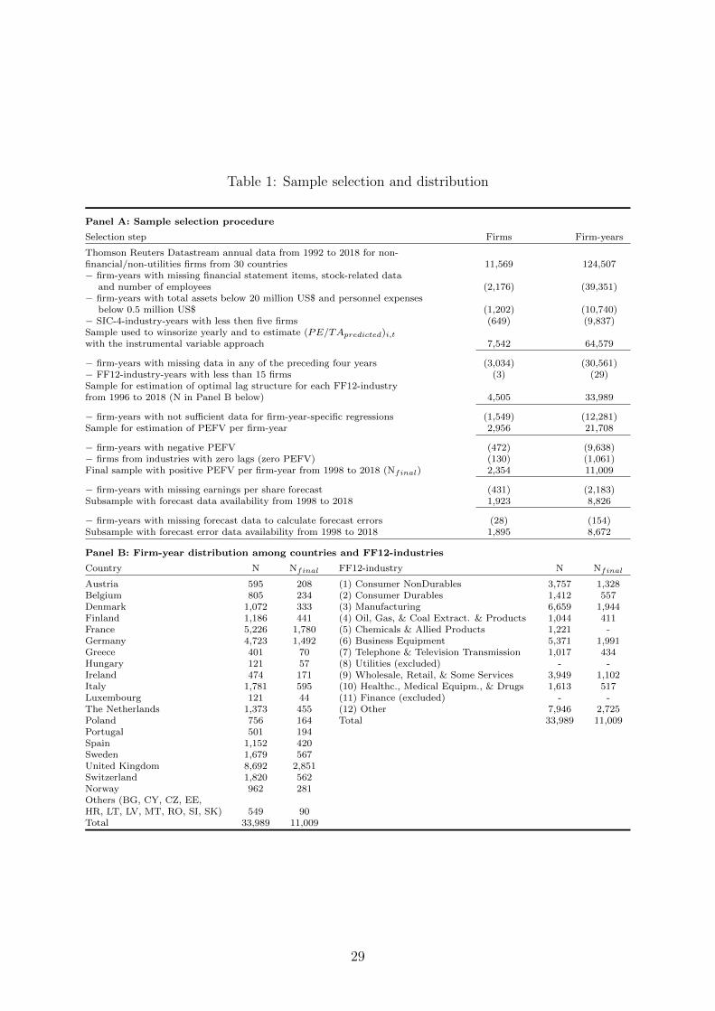
Table 1: Sample selection and distribution

Panel A: Sample selection procedure

Selection step Firms Firm-years

Thomson Reuters Datastream annual data from 1992 to 2018 for non-financial/non-utilities firms from 30 countries 11,569 124,507− firm-years with missing financial statement items, stock-related data

and number of employees (2,176) (39,351)− firm-years with total assets below 20 million US$ and personnel expenses

below 0.5 million US$ (1,202) (10,740)− SIC-4-industry-years with less then five firms (649) (9,837)Sample used to winsorize yearly and to estimate (PE/TApredicted)i,twith the instrumental variable approach 7,542 64,579

− firm-years with missing data in any of the preceding four years (3,034) (30,561)− FF12-industry-years with less than 15 firms (3) (29)Sample for estimation of optimal lag structure for each FF12-industryfrom 1996 to 2018 (N in Panel B below) 4,505 33,989

− firm-years with not sufficient data for firm-year-specific regressions (1,549) (12,281)Sample for estimation of PEFV per firm-year 2,956 21,708

− firm-years with negative PEFV (472) (9,638)− firms from industries with zero lags (zero PEFV) (130) (1,061)Final sample with positive PEFV per firm-year from 1998 to 2018 (Nfinal) 2,354 11,009

− firm-years with missing earnings per share forecast (431) (2,183)Subsample with forecast data availability from 1998 to 2018 1,923 8,826

− firm-years with missing forecast data to calculate forecast errors (28) (154)Subsample with forecast error data availability from 1998 to 2018 1,895 8,672

Panel B: Firm-year distribution among countries and FF12-industries

Country N Nfinal FF12-industry N Nfinal

Austria 595 208 (1) Consumer NonDurables 3,757 1,328Belgium 805 234 (2) Consumer Durables 1,412 557Denmark 1,072 333 (3) Manufacturing 6,659 1,944Finland 1,186 441 (4) Oil, Gas, & Coal Extract. & Products 1,044 411France 5,226 1,780 (5) Chemicals & Allied Products 1,221 -Germany 4,723 1,492 (6) Business Equipment 5,371 1,991Greece 401 70 (7) Telephone & Television Transmission 1,017 434Hungary 121 57 (8) Utilities (excluded) - -Ireland 474 171 (9) Wholesale, Retail, & Some Services 3,949 1,102Italy 1,781 595 (10) Healthc., Medical Equipm., & Drugs 1,613 517Luxembourg 121 44 (11) Finance (excluded) - -The Netherlands 1,373 455 (12) Other 7,946 2,725Poland 756 164 Total 33,989 11,009Portugal 501 194Spain 1,152 420Sweden 1,679 567United Kingdom 8,692 2,851Switzerland 1,820 562Norway 962 281Others (BG, CY, CZ, EE,HR, LT, LV, MT, RO, SI, SK) 549 90Total 33,989 11,009

29

Table 2: Lag structure regressions

Panel A: Cross-sectional regressions with different lag structures

Dependent variable:

OI/TAi,t

(1) (2) (3) (4)

(PE/TApredicted)i,t 0.664∗∗∗ 0.609∗∗∗ 0.566∗∗∗ 0.552∗∗∗

(0.038) (0.039) (0.039) (0.038)(PE/TApredicted)i,t−1 0.391∗∗∗ 0.164∗∗∗ 0.148∗∗∗ 0.113∗∗

(0.037) (0.046) (0.045) (0.046)(PE/TApredicted)i,t−2 0.296∗∗∗ 0.096∗∗ 0.079∗

(0.039) (0.046) (0.045)(PE/TApredicted)i,t−3 0.271∗∗∗ 0.079∗

(0.039) (0.044)(PE/TApredicted)i,t−4 0.270∗∗∗

(0.037)log(#E)i,t 0.016∗∗∗ 0.016∗∗∗ 0.016∗∗∗ 0.016∗∗∗

(0.001) (0.001) (0.001) (0.001)Intercept −0.034∗∗∗ −0.037∗∗∗ −0.038∗∗∗ −0.043∗∗∗

(0.009) (0.009) (0.009) (0.009)∑nk=1 βk/(1.1)k 0.355 0.394 0.417 0.412

Year dummies Yes Yes Yes YesFF12 dummies Yes Yes Yes YesRobust SEs Yes Yes Yes YesAIC -14286 -14366 -14435 -14508BIC -13983 -14054 -14114 -14179Observations 33,989 33,989 33,989 33,989Adjusted R2 0.355 0.357 0.358 0.360

Panel B: Optimal lag structure per FF12-industry

FF12-industry β0 β1 β2 β3∑nk=1 βk/(1.1)k R2

adj.

(1) Consumer NonDurables .586 .179 .274 .390 .176(2) Consumer Durables .957 .578 .526 .114(3) Manufacturing .455 .259 .122 .289 .554 .214(4) Oil, Gas, & Coal Extract. & Products .310 .451 .410 .260(5) Chemicals & Allied Products .833 - .120(6) Business Equipment .517 .524 .477 .209(7) Telephone & Television Transmission .623 .612 .556 .015(8) Utilities (excluded) - - - - - -(9) Wholesale, Retail, & Some Services .614 .139 .186 .292 .499 .330(10) Healthc., Medical Equipm., & Drugs .554 .499 .295 .697 .299(11) Finance (excluded) - - - - - -(12) Other .643 .136 .248 .328 .415

This table shows the derivation of the optimal lag structure per industry. Panel A reports results of cross-sectional regressionsfor different lag structures following equation (1). All variables are defined in Appendix A. Columns (1) to (4) present resultsfor one to four lags. Coefficients on industry dummies are not reported. Robust standard errors are shown in parentheses.*, **, *** denote statistical significance at the 0.10, 0.05, and 0.01 levels, respectively. Panel B reports the optimal lagstructure per industry where equation (1) is estimated industry-by-industry including year dummies for lag structures ofzero to four lags. Only lag structures where all coefficients are positive and significant on the one-sided ten percent levelare considered for the choice of the optimal model. The table reports coefficient estimates for the lag structure with thehighest explanatory power for each FF12-industry. The last two columns report the discounted sum of the coefficients forthe respective optimal lags and the adjusted R2.

30

Table 3: Descriptive statistics

Panel A: Characteristics of sample firms from 1992 to 2018

N Mean STD Min 25% Median 75% Max

TAi,t($m) 64,579 2,861 13,615 20 80 239 998 397,812PEi,t($m) 64,579 417 1,524 0.5 17 52 197 40,950

PE/TAi,t 64,579 0.27 0.21 0.01 0.13 0.23 0.36 1.33(PE/TApredicted)i,t 64,579 0.27 0.13 −0.30 0.18 0.26 0.34 1.28OI/TAi,t 64,579 0.37 0.25 −0.25 0.21 0.33 0.49 1.57

PE/SALESi,t 64,579 0.30 0.36 0.02 0.15 0.24 0.34 6.08CAPEX/SALESi,t 63,794 0.09 0.19 0.00 0.02 0.04 0.07 1.98

Panel B: Descriptive statistics of final sample with positive PEFV

N Mean STD Min 25% Median 75% Max

TAi,t($m) 11,009 5,540 21,649 20 177 517 2,459 396,812PEi,t($m) 11,009 729 2,089 0.5 43 120 449 38,762

PEFVi,t 11,009 2.08 2.04 0.00 0.50 1.28 3.03 6.51PE/TAi,t 11,009 0.28 0.22 0.01 0.13 0.23 0.36 1.33PEFV ∗ PE/TAi,t 11,009 0.49 0.53 0.00 0.09 0.26 0.75 1.64

Pi,t/Pi,t−1 11,009 1.09 0.47 0.07 0.81 1.04 1.30 5.32OIPSi,t/Pi,t−1 11,009 0.63 0.57 0.07 0.22 0.43 0.84 2.19PEPSi,t/Pi,t−1 11,009 0.56 0.56 0.05 0.16 0.35 0.76 2.09PEFVi,t/Pi,t−1 11,009 0.48 0.70 0.00 0.03 0.12 0.56 2.21EPSi,t/Pi,t−1 8,826 0.07 0.05 −0.06 0.04 0.07 0.10 0.18SGAPSi,t/Pi,t−1 7,164 0.44 0.45 0.03 0.12 0.27 0.57 1.70RNDPSi,t/Pi,t−1 11,009 0.02 0.03 0.00 0.00 0.00 0.01 0.13

|FEi,t|/Pi,t−1 8,672 0.04 0.10 0.00 0.01 0.01 0.04 1.46FEi,t/Pi,t−1 8,672 0.01 0.10 −0.40 −0.02 −0.004 0.01 1.30#Analystsi,t 8,672 8.22 7.81 1 2 5 12 44

This table reports descriptive statistics for different samples. Panel A reports characteristics for the initial sample of firmsfrom 1992 to 2018 and Panel B reports descriptive statistics for the final sample with positive PEFV.

31

Tab

le4:

Fir

mch

arac

teri

stic

san

dPEFV

Dep

enden

tva

riabl

e:

PEFV−Decile i,t

(1)

(2)

(3)

(4)

(5)

(6)

(7)

log(#E

) i,t

−0.

029∗

∗∗−

0.0

30∗

∗∗−

0.0

35∗

∗∗

(0.0

02)

(0.0

02)

(0.0

10)

MTBi,t

0.00

6∗∗

∗0.0

07∗∗

∗

(0.0

02)

(0.0

02)

Tangibility i,t

−0.0

59∗∗

∗−

0.0

37

(0.0

22)

(0.0

23)

PE/TAi,t

0.0

76∗∗

∗0.0

80∗∗

∗

(0.0

23)

(0.0

24)

MeanPay i,t

0.0

01∗

∗∗0.0

0004

(0.0

001)

(0.0

001)

TrainingDays i,t

(%)

0.0

20∗

(0.0

12)

Intercept

0.89

1∗∗

∗0.

629∗∗

∗0.6

70∗

∗∗0.6

33∗∗

∗0.6

30∗

∗∗0.8

72∗∗

∗0.8

38∗∗

∗

(0.0

31)

(0.0

19)

(0.0

21)

(0.0

18)

(0.0

16)

(0.0

33)

(0.0

94)

FF

12d

um

mie

sY

esY

esY

esY

esY

esY

esY

es

Yea

rd

um

mie

sY

esY

esY

esY

esY

esY

esY

es

Ob

serv

atio

ns

11,0

0910

,627

11,0

08

11,0

09

11,0

09

10,6

26

1,0

13

Ad

just

edR

20.

089

0.06

00.0

59

0.0

60

0.0

62

0.0

97

0.1

33

Th

ista

ble

rep

ort

sth

ere

sult

sof

OL

Sre

gre

ssio

nofPEFV−Decile i

,ton

hu

man

-cap

ital-

rela

ted

firm

chara

cter

isti

cs.

All

vari

ab

les

are

defi

ned

inA

pp

end

ixA

.In

du

stry

an

dyea

rd

um

mie

sare

not

show

n.

Tw

o-w

ay-c

lust

erro

bu

stst

an

dard

erro

rs,

clu

ster

ing

at

the

firm

an

dyea

rle

vel

s,are

show

nin

pare

nth

eses

.*,

**,

***

den

ote

stati

stic

al

sign

ifica

nce

at

the

0.1

0,

0.0

5,

an

d0.0

1le

vel

s,re

spec

tivel

y.

32

Tab

le5:

PEFV

and

conte

mp

oran

eous

stock

pri

ces

Dep

enden

tva

riabl

e:

Pi,t/Pi,t−

1

(1)

(2)

(3)

(4)

(5)

(6)

(7)

(8)

OIPSi,t/P

i,t−

10.

735∗

∗∗0.

712∗

∗∗0.7

17∗∗

∗0.6

31∗

∗∗0.3

32∗∗

∗0.3

97∗∗

∗0.4

61∗∗

∗0.3

36∗∗

∗

(0.0

58)

(0.0

58)

(0.0

59)

(0.0

51)

(0.0

73)

(0.0

95)

(0.0

96)

(0.0

74)

PEPSi,t/P

i,t−

1−

0.53

2∗∗∗

−0.

506∗

∗∗−

0.5

21∗

∗∗−

0.5

18∗∗

∗−

0.2

36∗∗

∗−

0.3

30∗

∗∗−

0.0

49

−0.2

30∗∗

∗

(0.0

42)

(0.0

57)

(0.0

56)

(0.0

45)

(0.0

73)

(0.0

99)

(0.1

18)

(0.0

73)

PEFV

i,t/Pi,t-1

0.0

55**

0.0

43**

0.0

46**

0.0

41*

0.0

73***

(0.0

22)

(0.0

21)

(0.0

19)

(0.0

22)

(0.0

27)

PEFV-D

ecilei,t

0.0

53**

(0.0

25)

EPSi,t/P

i,t−

12.1

36∗∗

∗2.0

90∗∗

∗2.7

67∗∗

∗2.1

32∗∗

∗

(0.2

42)

(0.2

59)

(0.3

76)

(0.2

42)

SGAPSi,t/P

i,t−

10.0

71∗∗

∗

(0.0

23)

RNDPSi,t/P

i,t−

11.3

76∗∗

∗

(0.3

22)

log(#E

) i,t

−0.

012∗

∗∗−

0.01

3∗∗∗

−0.0

06

−0.0

05

−0.0

10∗∗

−0.0

09∗

−0.1

05∗∗

∗−

0.0

15∗∗

∗

(0.0

03)

(0.0

04)

(0.0

05)

(0.0

05)

(0.0

05)

(0.0

05)

(0.0

15)

(0.0

04)

Intercept

1.03

3∗∗∗

1.03

7∗∗∗

0.9

62∗∗

∗1.1

85∗

∗∗1.0

73∗∗

∗1.0

24∗∗

∗2.0

20∗∗

∗1.0

89∗∗

∗

(0.0

58)

(0.0

55)

(0.0

56)

(0.0

69)

(0.0

55)

(0.0

59)

(0.1

49)

(0.0

50)

FF

12d

um

mie

sY

esY

esY

esY

esY

ear

du

mm

ies

Yes

Yes

Yes

Yes

Yes

Fir

md

um

mie

sY

esO

bse

rvat

ion

s21

,708

11,0

0911,0

09

11,0

09

8,8

26

5,9

60

8,8

26

8,8

26

Ad

just

edR

20.

097

0.09

50.1

00

0.3

41

0.4

11

0.4

20

0.4

91

0.4

09

Th

ista

ble

rep

ort

sth

ere

sult

sof

OL

Sre

gre

ssio

nof

conte

mp

ora

neo

us

stock

pri

ceonPEFV

follow

ing

equ

ati

on

(3).

All

vari

ab

les

are

defi

ned

inA

pp

end

ixA

.C

olu

mn

s(1

)an

d(2

)sh

ow

the

sam

ple

red

uct

ion

from

all

firm

-yea

rsw

her

ePEFV

isca

lcu

late

dto

all

firm

-yea

rsw

ithPEFV

larg

erth

an

zero

.C

olu

mn

(3)

pre

sents

the

incl

usi

on

ofPEFV

an

dco

lum

n(4

)sh

ow

sth

eeff

ect

of

incl

ud

ing

ind

ust

ryan

dyea

rd

um

mie

s.In

colu

mn

s(5

)to

(8),

the

sam

ple

isfu

rth

erre

du

ced

regard

ing

an

aly

stea

rnin

gs

per

share

fore

cast

availab

ilit

y.C

olu

mn

(6)

pre

sents

the

incl

usi

on

of

contr

ols

for

SG

&A

per

share

an

dR

&D

per

share

as

inB

an

ker

etal.

(2019).

Colu

mn

(7)

show

sre

sult

sfo

rfi

rman

dyea

rd

um

mie

s.C

olu

mn

(8)

show

sd

eciles

ofPEFV

resc

ale

dto

ran

ge

from

zero

toon

eas

an

alt

ern

ati

ve

mea

sure

.T

wo-w

ay-c

lust

erro

bu

stst

an

dard

erro

rs,

clu

ster

ing

at

the

firm

an

dyea

rle

vel

s,are

show

nin

pare

nth

eses

.In

du

stry

,yea

ran

dfi

rmd

um

mie

sare

not

show

n.

*,

**,

***

den

ote

stati

stic

al

sign

ifica

nce

at

the

0.1

0,

0.0

5,

an

d0.0

1le

vel

s,re

spec

tivel

y.

33

Table 6: PEFV and contemporaneous forecast errors

Dependent variable:

|FEi,t|/Pi,t−1 FEi,t/Pi,t−1

(1) (2) (3) (4) (5) (6) (7)

PEFV i,t /Pi,t-1 0.013*** 0.017*** 0.015*** 0.005** 0.006** 0.006**

(0.002) (0.003) (0.004) (0.002) (0.002) (0.003)

PEFV-Decilei,t 0.010***

(0.003)OIPSi,t/Pi,t−1 −0.175∗∗∗ −0.205∗∗∗

(0.033) (0.031)PEPSi,t/Pi,t−1 0.211∗∗∗ 0.218∗∗∗

(0.038) (0.036)∆OIPSi,t/Pi,t−1 −0.041 −0.047 −0.081∗∗ −0.078∗∗ −0.080∗∗

(0.036) (0.033) (0.035) (0.031) (0.035)∆PEPSi,t/Pi,t−1 −0.052 −0.050 0.017 −0.013 0.015

(0.053) (0.034) (0.049) (0.033) (0.048)∆SGAPSi,t/Pi,t−1 −0.018 0.005

(0.022) (0.023)∆RNDPSi,t/Pi,t−1 −0.415∗∗∗ −0.319∗∗

(0.116) (0.142)log(#Analysts)i,t −0.001 −0.012∗∗∗ −0.011∗∗∗ 0.001 −0.003 −0.002 −0.004∗

(0.002) (0.002) (0.003) (0.002) (0.002) (0.002) (0.002)log(#E)i,t −0.004∗∗∗ 0.0004 −0.0001 −0.005∗∗∗ −0.003∗∗∗ −0.004∗∗∗ −0.004∗∗∗

(0.002) (0.001) (0.001) (0.002) (0.001) (0.001) (0.001)Intercept 0.060∗∗∗ 0.048∗∗∗ 0.059∗∗∗ 0.036∗∗∗ 0.027∗∗∗ 0.029∗∗∗ 0.026∗∗∗

(0.010) (0.008) (0.010) (0.007) (0.006) (0.010) (0.006)

Observations 8,672 8,672 5,739 8,672 8,672 5,739 8,672Adjusted R2 0.158 0.100 0.118 0.113 0.055 0.066 0.055

This table reports the results of OLS regression of contemporaneous forecast errors on PEFV. All variables are definedin Appendix A. Absolute forecast errors are the dependent variable in columns (1) to (3). Signed forecast errors arethe dependent variable in columns (4) to (7). Column (7) shows deciles of PEFV rescaled to range from zero to oneas an alternative measure. Two-way-cluster robust standard errors, clustering at the firm and year levels, are shown inparentheses. Industry and year dummies are not shown. *, **, *** denote statistical significance at the 0.10, 0.05, and 0.01levels, respectively.

34

Tab

le7:

Futu

rem

onth

lyre

turn

sin

the

year

from

July

toJune

afte

rp

ortf

olio

form

atio

n

PEFV

PEFV

∗PE/TA

1st

2nd

3rd

4th

5th

LS

1st

2nd

3rd

4th

5th

LS

PanelA

:Valu

e-w

eig

hted:

Intercept

−.05

.18

.20

.11

.49∗∗∗

.54∗∗∗

−.06

.06

.03

.55∗∗∗

.59∗∗∗

.65∗∗∗

(.10)

(.12)

(.16)

(.19)

(.14)

(.18)

(.09)

(.12)

(.12)

(.16)

(.18)

(.22)

Rm,τ

−Rf,τ

1.06∗∗∗

1.01∗∗∗

1.06∗∗∗

1.03∗∗∗

.97∗∗∗

−.09∗

1.02∗∗∗

1.02∗∗∗

1.00∗∗∗

1.00∗∗∗

1.06∗∗∗

.03

(.03)

(.03)

(.04)

(.05)

(.03)

(.05)

(.03)

(.03)

(.03)

(.04)

(.04)

(.05)

SM

Bτ

.15∗∗

.12∗

.23∗∗∗

.12

.002

−.15

.10∗

.07

.25∗∗∗

−.01

.42∗∗∗

.31∗∗∗

(.06)

(.07)

(.09)

(.11)

(.08)

(.10)

(.06)

(.08)

(.07)

(.09)

(.09)

(.11)

HM

Lτ

−.05

−.10

−.49∗∗∗

−.45∗∗∗

−.27∗∗∗

−.22

−.005

−.06

−.09

−.49∗∗∗

−.55∗∗∗

−.54∗∗∗

(.10)

(.10)

(.14)

(.17)

(.10)

(.16)

(.10)

(.10)

(.09)

(.10)

(.14)

(.17)

RM

Wτ

.15

.08

−.32∗∗

−.17

−.02

−.16

.22∗∗

.06

.02

−.32∗∗

−.17

−.38∗

(.10)

(.11)

(.14)

(.17)

(.13)

(.17)

(.10)

(.09)

(.10)

(.15)

(.15)

(.20)

CM

Aτ

.23∗∗

.24∗∗

.26∗

−.03

−.02

−.25

.20∗

.35∗∗∗

.28∗∗

−.07

−.03

−.23

(.11)

(.12)

(.15)

(.19)

(.12)

(.17)

(.11)

(.13)

(.11)

(.14)

(.16)

(.21)

Obse

rvations

228

228

228

228

228

228

228

228

228

228

228

228

Adju

sted

R2

.92

.91

.84

.81

.88

.09

.93

.90

.89

.85

.84

.20

5th-1st

.54***

(.1

7)

Annualized:

6.5

%.6

5***

(.2

1)

Annualized:

7.8

%

PanelB:Equal-weig

hted:

Intercept

−.12

.15

.25∗∗∗

−.03

.17∗

.29∗∗∗

−.15∗

.04

.11

.17∗

.25∗∗

.40∗∗∗

(.08)

(.10)

(.10)

(.10)

(.10)

(.11)

(.08)

(.09)

(.09)

(.10)

(.11)

(.12)

Rm,τ

−Rf,τ

1.02∗∗∗

1.00∗∗∗

.99∗∗∗

1.01∗∗∗

.99∗∗∗

−.02

1.01∗∗∗

.98∗∗∗

.98∗∗∗

1.05∗∗∗

1.00∗∗∗

−.02

(.02)

(.03)

(.02)

(.02)

(.02)

(.03)

(.02)

(.02)

(.02)

(.02)

(.03)

(.03)

SM

Bτ

.78∗∗∗

.88∗∗∗

.74∗∗∗

.91∗∗∗

.82∗∗∗

.03

.70∗∗∗

.84∗∗∗

.82∗∗∗

.87∗∗∗

.92∗∗∗

.23∗∗∗

(.04)

(.04)

(.05)

(.05)

(.05)

(.06)

(.04)

(.04)

(.04)

(.05)

(.06)

(.07)

HM

Lτ

.27∗∗∗

.14∗

.17∗∗

.25∗∗∗

.13∗∗

−.13∗

.31∗∗∗

.27∗∗∗

.20∗∗∗

.06

.13

−.18∗∗

(.06)

(.08)

(.07)

(.07)

(.06)

(.07)

(.05)

(.08)

(.06)

(.08)

(.09)

(.08)

RM

Wτ

.20∗∗∗

.10

.01

.19∗∗

.11

−.09

.26∗∗∗

.14∗∗

.11

.04

.08

−.18∗

(.06)

(.08)

(.08)

(.08)

(.07)

(.09)

(.06)

(.07)

(.07)

(.09)

(.09)

(.10)

CM

Aτ

.09

−.02

−.04

−.07

−.08

−.17∗

.08

.01

−.09

.01

−.13

−.21∗

(.08)

(.11)

(.08)

(.10)

(.09)

(.09)

(.07)

(.11)

(.09)

(.10)

(.11)

(.11)

Obse

rvations

228

228

228

228

228

228

228

228

228

228

228

228

Adju

sted

R2

.96

.94

.95

.95

.94

.08

.95

.95

.95

.94

.93

.18

5th-1st

.29**

(.1

3)

Annualized:

3.5

%.4

0***

(.1

4)

Annualized:

4.8

%

Th

ista

ble

rep

ort

sm

onth

lyab

norm

al

retu

rns

of

port

foli

os

bu

ilt

aro

un

dtw

om

easu

res

of

the

futu

rein

tan

gib

leass

etvalu

eofPE

follow

ing

equ

ati

on

(4).

All

vari

ab

les

are

defi

ned

inA

pp

end

ixA

.P

ort

folios

are

form

edat

the

end

of

Ju

ne

each

yea

rt+

1by

ass

ign

ing

firm

sin

tofi

ve

qu

inti

les

base

donPEFV

orPEFV*PE/TA

.PEFV

an

dPEFV*PE/TA

are

mea

sure

dat

firm

s’fi

scal

yea

ren

din

gin

yea

rt.

Rob

ust

stan

dard

erro

rsare

show

nin

pare

nth

eses

.*,

**,

***

den

ote

stati

stic

al

sign

ifica

nce

at

the

0.1

0,

0.0

5,

an

d0.0

1le

vel

s,re

spec

tivel

y.

35

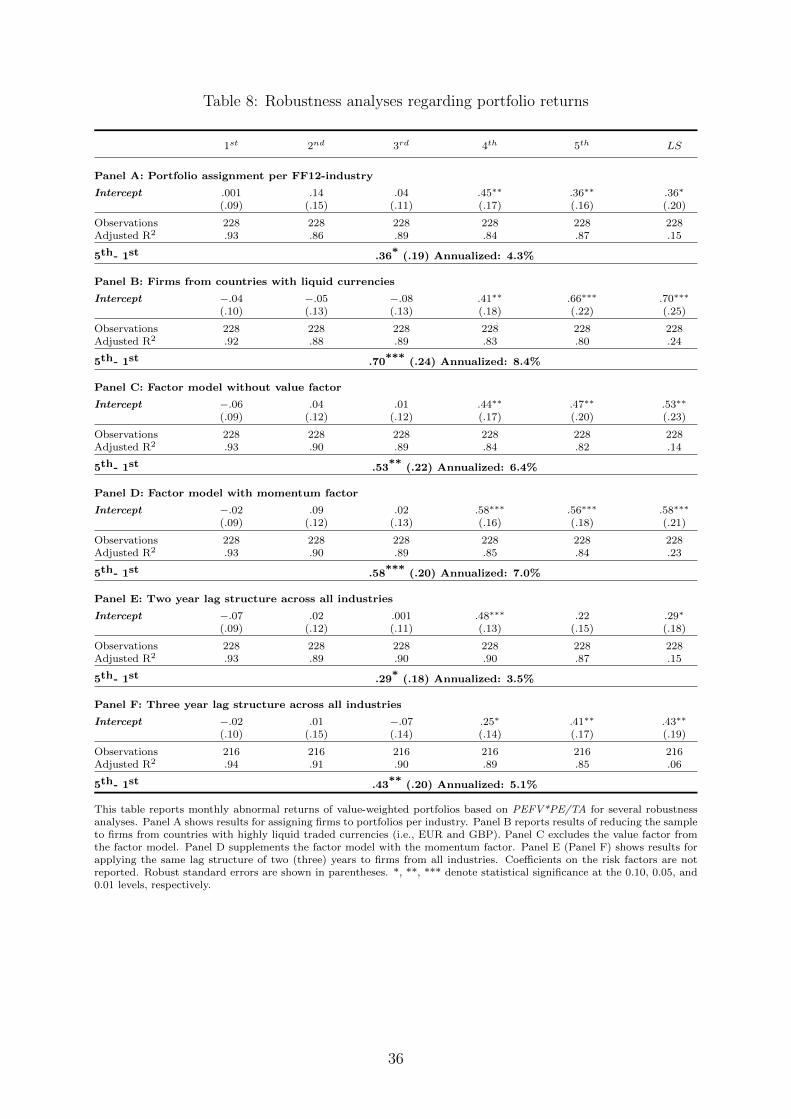
Table 8: Robustness analyses regarding portfolio returns

1st 2nd 3rd 4th 5th LS

Panel A: Portfolio assignment per FF12-industry

Intercept .001 .14 .04 .45∗∗ .36∗∗ .36∗

(.09) (.15) (.11) (.17) (.16) (.20)

Observations 228 228 228 228 228 228Adjusted R2 .93 .86 .89 .84 .87 .15

5th- 1st .36* (.19) Annualized: 4.3%

Panel B: Firms from countries with liquid currencies

Intercept −.04 −.05 −.08 .41∗∗ .66∗∗∗ .70∗∗∗

(.10) (.13) (.13) (.18) (.22) (.25)

Observations 228 228 228 228 228 228Adjusted R2 .92 .88 .89 .83 .80 .24

5th- 1st .70*** (.24) Annualized: 8.4%

Panel C: Factor model without value factor

Intercept −.06 .04 .01 .44∗∗ .47∗∗ .53∗∗

(.09) (.12) (.12) (.17) (.20) (.23)

Observations 228 228 228 228 228 228Adjusted R2 .93 .90 .89 .84 .82 .14

5th- 1st .53** (.22) Annualized: 6.4%

Panel D: Factor model with momentum factor

Intercept −.02 .09 .02 .58∗∗∗ .56∗∗∗ .58∗∗∗

(.09) (.12) (.13) (.16) (.18) (.21)

Observations 228 228 228 228 228 228Adjusted R2 .93 .90 .89 .85 .84 .23

5th- 1st .58*** (.20) Annualized: 7.0%

Panel E: Two year lag structure across all industries

Intercept −.07 .02 .001 .48∗∗∗ .22 .29∗

(.09) (.12) (.11) (.13) (.15) (.18)

Observations 228 228 228 228 228 228Adjusted R2 .93 .89 .90 .90 .87 .15

5th- 1st .29* (.18) Annualized: 3.5%

Panel F: Three year lag structure across all industries

Intercept −.02 .01 −.07 .25∗ .41∗∗ .43∗∗

(.10) (.15) (.14) (.14) (.17) (.19)

Observations 216 216 216 216 216 216Adjusted R2 .94 .91 .90 .89 .85 .06

5th- 1st .43** (.20) Annualized: 5.1%

This table reports monthly abnormal returns of value-weighted portfolios based on PEFV*PE/TA for several robustnessanalyses. Panel A shows results for assigning firms to portfolios per industry. Panel B reports results of reducing the sampleto firms from countries with highly liquid traded currencies (i.e., EUR and GBP). Panel C excludes the value factor fromthe factor model. Panel D supplements the factor model with the momentum factor. Panel E (Panel F) shows results forapplying the same lag structure of two (three) years to firms from all industries. Coefficients on the risk factors are notreported. Robust standard errors are shown in parentheses. *, **, *** denote statistical significance at the 0.10, 0.05, and0.01 levels, respectively.

36

Table 9: Long-term portfolio returns

Year 1

1st 2nd 3rd 4th 5th

Intercept −.06 .06 .03 .55∗∗∗ .59∗∗∗

(.09) (.12) (.12) (.16) (.18)

Observations 228 228 228 228 228Adjusted R2 .93 .90 .89 .85 .84

5th- 1st .65*** (.21) Annualized: 7.8%

Year 2

1st 2nd 3rd 4th 5th

Intercept −.03 .04 .14 .55∗∗∗ .40∗∗

(.11) (.14) (.14) (.16) (.16)

Observations 216 216 216 216 216Adjusted R2 .93 .88 .89 .83 .87

5th- 1st .43** (.19) Annualized: 5.1%

Year 3

1st 2nd 3rd 4th 5th

Intercept −.0004 .14 −.04 .37∗∗ .25(.10) (.14) (.12) (.17) (.16)

Observations 204 204 204 204 204Adjusted R2 .93 .89 .92 .89 .85

5th- 1st .25 (.19) Annualized: 3.1%

This table reports monthly abnormal returns of value-weighted portfolios based on PEFV*PE/TA up to the third yearafter portfolio formation following the same procedure as in Table 7. Coefficients on the risk factors are not reported.Robust standard errors are shown in parentheses. *, **, *** denote statistical significance at the 0.10, 0.05, and 0.01 levels,respectively.

37

Table 10: Cross-sectional future monthly returns

Dependent variable:

(Ri,τ −Rf,τ )t+1 (Ri,τ −RInd,τ )t+1

(1) (2) (3) (4) (5) (6)

PEFV-Quintilei,t .085*** .081*** .080***

(.026) (.030) (.030)

PEFV*PE/TA-Quintilei,t .210*** .168*** .167***

(.029) (.036) (.036)Momentum−1,0 −.032∗∗∗ −.033∗∗∗ −.034∗∗∗ −.034∗∗∗ −.036∗∗∗ −.037∗∗∗

(.007) (.007) (.008) (.008) (.008) (.008)Momentum−12,−1 .007∗ .006 .004 .004 .004 .003

(.004) (.004) (.005) (.005) (.005) (.005)Accrualsi,t .015 −.008 −.200 −.200 −.186 −.199

(.145) (.144) (.181) (.182) (.182) (.182)AssetGrowthi,t −.157 −.153 −.423∗ −.409∗ −.410∗ −.391∗

(.181) (.182) (.216) (.216) (.210) (.209)log(BE/ME)i,t .380∗∗∗ .460∗∗∗ .604∗∗∗ .640∗∗∗ .607∗∗∗ .645∗∗∗

(.075) (.075) (.092) (.093) (.087) (.089)log(ME)i,t .287∗∗∗ .329∗∗∗ .309∗∗∗ .332∗∗∗ .306∗∗∗ .329∗∗∗

(.036) (.038) (.041) (.042) (.041) (.042)SGA/TAi,t .568∗ .354 .519∗ .299

(.304) (.309) (.309) (.315)RND/TAi,t 5.272∗∗∗ 4.641∗∗∗ 5.195∗∗∗ 4.676∗∗∗

(1.561) (1.551) (1.441) (1.458)EBITDA/TAi,t 2.424∗∗∗ 2.420∗∗∗ 2.395∗∗∗ 2.411∗∗∗

(.685) (.689) (.663) (.669)Intercept −1.241∗∗∗ −1.844∗∗∗ −1.608∗∗∗ −1.940∗∗∗ −2.325∗∗∗ −2.667∗∗∗

(.437) (.430) (.501) (.498) (.446) (.454)

Observations 109,908 109,908 72,824 72,824 72,824 72,824R2 .290 .291 .310 .311 .093 .094

This table reports results from average Fama and MacBeth (1973) regression coefficients for monthly returns regressed onvarious firm and return characteristics. The monthly returns are from July t+1 to June t+2. *, **, *** denote statisticalsignificance at the 0.10, 0.05, and 0.01 levels, respectively.

38

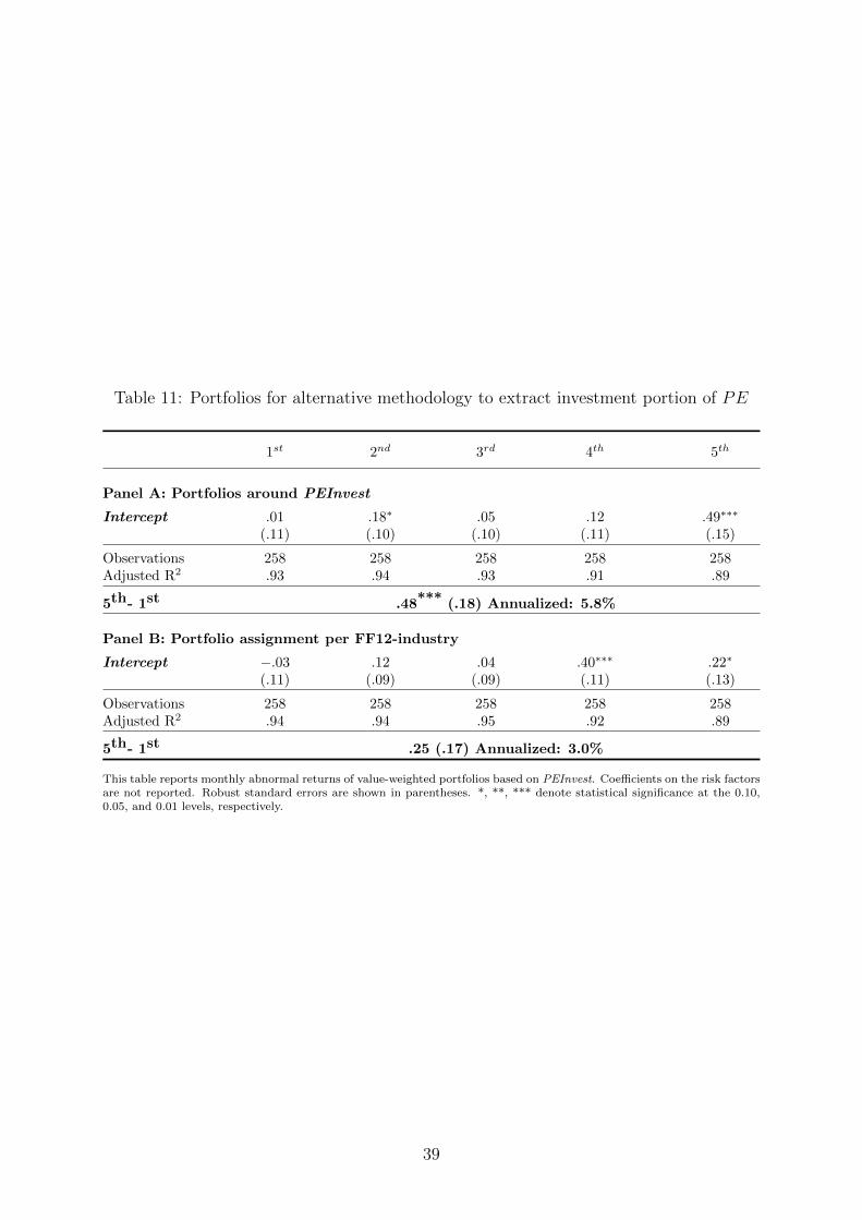
Table 11: Portfolios for alternative methodology to extract investment portion of PE

1st 2nd 3rd 4th 5th

Panel A: Portfolios around PEInvest

Intercept .01 .18∗ .05 .12 .49∗∗∗

(.11) (.10) (.10) (.11) (.15)

Observations 258 258 258 258 258Adjusted R2 .93 .94 .93 .91 .89

5th- 1st .48*** (.18) Annualized: 5.8%

Panel B: Portfolio assignment per FF12-industry

Intercept −.03 .12 .04 .40∗∗∗ .22∗

(.11) (.09) (.09) (.11) (.13)

Observations 258 258 258 258 258Adjusted R2 .94 .94 .95 .92 .89

5th- 1st .25 (.17) Annualized: 3.0%

This table reports monthly abnormal returns of value-weighted portfolios based on PEInvest. Coefficients on the risk factorsare not reported. Robust standard errors are shown in parentheses. *, **, *** denote statistical significance at the 0.10,0.05, and 0.01 levels, respectively.

39