Journal of Aquatic Ecosystem Health 2: 197-204, 1993. © 1993 KluwerAcademic Publishers. Printed in the Netherlands.

The statistical implications of autocorrelation for detection in environmental health assessment

M. Power Department of Agricultural Economics, University of Manitoba, Winnipeg, Manitoba, R3T 2N2, Canada

Keywords: environmental assessment, detection, time series analysis, non-stationarity

Abstract. Many environmental health and risk assessment techniques and models aim at estimating the fluctuations of selected biological endpoints through the time domain as a means of assessing changes in the environment or the probability of a particular measurement level occurring. In either case, estimates of the sample variance and mean of the sample variance are crucial to making appropriate statistical inferences. The commonly employed statistical techniques for estimating both measures presume the data were generated by a covariance stationary process. In such cases, the observations are treated as independently and identically distributed and classical statistical testing methods are applied. However, if the assumption of covariance stationarity is violated, the resulting sample variance and variance of the sample mean estimates are biased. The bias compromises statistical testing procedures by increasing the probability of detecting significance in tests of mean and variance differences. This can lead to inappropriate decisions being made about the severity of environmental damage. Accordingly, it is argued that data sets be examined for correlation in the time domain and appropriate adjustments be made to the required estimators before they are used in statistical hypothesis testing. Only then can credible and scientifically defensible decisions be made by environmental decision makers and regulators.

1. Introduction

The dynamic complexity of natural ecosystems makes them ideal subjects for the modeller 's art. Work by Ferson et al. (1989), Bartell et al. (1992), Minns (1992) and Barnthouse (1992) have all recommended the use of modelling as a means of representing, controlling, and studying the complex web of inter-relationships that comprise terrestrial and aquatic environments. Minns (1992) recommends that 'Modelling be undertaken with existing data and ideas before new research and data collection begins ' . Barnthouse (1992) has concluded that models will play a 'critical role' in providing ecological risk assessors with con- sistent and credible assessments of ecological risks, and Bartell et al. (1992) view modelling as an effective and credible means of producing scientifically sound environmental assessment techniques for use by environmental decision makers and regulators.

The stochastic nature of many basic biological phenomena (e.g. population abundance, biomass, and recruitment) further argue that modelling, and

particularly computer based simulation modelling, holds great explanatory and predictive promise where environmental and risk assessment are concerned. Despite that promise, modelling, like all methodologies, has its drawbacks. Chief among them are the incidence of correlation between data points in the time domain (autocorrelation) and the implications such correlation holds for parameter estimation. This paper discusses the statistical aspects of the problem and the consequent diffi- culties autocorrelation poses for detection in environmental health and risk assessment.

2. The stationarity assumption

Environmental health and risk assessment models aim at estimating the fluctuations of selected bio- logical endpoints in the time domain as a means of (1) characterizing the relative health of an ecosystem, or, (2) assessing the probability of observing a particular environmental response to anthropogenic stress. One important endpoint is the decline in temporal mean abundance. Emlen

198

(1989) recommends it as a biologically important and regulatory significant endpoint. Bartell et al .

(1992) focus on population fluctuations in the development of a comprehensive environmental risk assessment methodology. Numerous other examples of the concern about population change through time are given in Barnthouse (1992). Regardless of the endpoint chosen, time dependent assessments and models produce a series of obser- vations X1 . . . . . X~, for time periods 1 . . . . . n, typically used as inputs to statistical descriptions of either the relative environmental health of an area or the risk associated with a specified action. Data displaying both randomness and variability may be regarded as the output of a stochastic process. A stochastic process is defined as a collection of random variables {Xt , t ~ T } all defined on a common sample space (Ross, 1985, p. 2), e.g. population abundance. In time series modelling, t is equated with time and T is the index set determining the number of random variables in the data collection under study. If T is countable, it is referred to as a discrete-time stochastic process. In effect, any time ordered or sequential set of observations (X~ . . . . . X,) can be treated as the product of a stochastic process. Such processes may be described by the n-dimen- sional probability distribution (Box & Jenkins, 1976):

p(x~, x~ . . . . . x . ) . ( 1 )

If joint normality is assumed in the n-dimensional distribution, it may be succinctly described by its n means ( E ( X I ) , . . . E ( X n ) ) , its n variances (Var(X1) . . . . . Var(X,)) and its n(n - 1)/2 co- variances (Cov(XiXj); i < j) .

One cannot, however, infer the general proba- bility structure of an n-dimensional probability distribution from a single realization of the process (Abraham & Ledolter, 1983) which, in practice, is all that is available for study. That is because there are only n observations available to estimate n + n ( n + 1)/2 unknown parameters. Simplifying assumptions are used to overcome the indetermi- nacy problem, the most powerful of which is stationarity. Stationary processes are a special class of processes for which the probability dis- tribution [p(X)] at times t~ . . . . . tm is identical to the distribution at times tt + ~ . . . . . tm+ ~, where k

is an arbitrary shift along the time axis. More formally, the conditions for stationarity may be expressed as follows (Law & Kelton, 1991):

E(X i ) = ~L i = ~t f o r i = 1 , 2 . . . a n d - o o < g < o o ; (2)

Var(Xi) = oi 2 = 0 2 f o r i = 1 , 2 . . . a n d o 2<o% (3)

Ci, ~+; = Cov(X~, Xi+j) is independent of i for j = 1, 2 . . . . (4)

That is to say, the mean and variance are time independent and have common values g and o 2, respectively. Furthermore, the covariance between any two observations, Xi and X i + j, depends only on the separation, j, not on the actual time values at i and i + j .

Given X 1 . . . . . Xn identically and independently distributed (IID) observations with finite popula- tion mean and variance, the usual objectives are to estimate I.t and o 2 with X ( n ) and S2(n) , the unbiased sample mean and variance estimators (Hogg & Craig, 1978). i~'(n) is itself a random variable in so far as it is the product of a single realization of the stochastic process being consid- ered. It will have a variance o2[,Y(n)] which can be used to assess how close X ( n ) is to the population parameter g. The variance of X(n) may be written as fo l lows :

l~2[.~(n)] (~2[ ~ Xi] (~.2 . . . . . ( 5 )

i = l n n

Furthermore, because o2[_.~(n)] is a population parameter, and therefore unknown, it must be esti- mated by 62[~'(n)], the variance of the observed .~(n) values, as follows:

62[~'(n)] - S2(n) (6) n

In both (5) and (6) above, if the Xi's are indepen- dent, then they are uncorrelated. Thus, the corre- lation coefficient, Pj = 0 for j = 0, 1 . . . . . n - 1, may be written as

C,,,+j Cj _ Cj j = 0 , 1 ,2 . . . . (7) PJ-~] 2 2 O2 - Co (Yi (~i+j

where Ci, i+j = covariance between X,, and Xi+j.

3. The effects of correlation

The above is the standard approach to estimation of the population variance and variance of the mean parameters for time dependent data. It is, however, built on the strong assumption of inde- pendence. Engineering and economic system studies have shown that many systems, especially perturbed systems, violate the independence assumption by being correlated in time (Koutsoyiannis, 1977; Draper & Smith, 1981; Law & Kelton, 1991). Even if the system was originally stationary, perturbations may well have destroyed the stationarity and, in the immediate post-pertur- bation period, the system will almost invariably display autocorrelative behaviour (Law & Kelton, 1991). In such cases, the X1 . . . . . Xn observations can no longer be said to be IID because the existence of correlations between the X 1 , . . . , Xn observations violates the independence assump- tion. While the violation of the independence assumption does not affect the unbiasedness of the sample mean as an estimator of bt, S2(n) can no longer be regarded as an unbiased estimator of cyZ(n) (Ross, 1985). In such cases, questions immediately arise as to the extent of the bias and its implications for hypothesis testing.

Anderson (1971) has shown that the expected value of S2(n), when the Xi values are correlated with respect to time, will be as follows:

[ ' ] E[S2(n)]=cy2 1 2j=1 n - ] (8)

I f P j = 0 f o r j = l , 2 , . . . , n - l ( t h e c a s e o f i n d e - pendence), then E[S2(n)] collapses to (~2 and the estimate of cy 2, S2(n) will be unbiased. On the other hand, if Pj is greater or less than 0, then positive (Pj > 0) or negative (Pj < 0) correlation exists and the E[S2(n)] will be less or greater than cy 2 as Pj is greater or less than zero. That implies that the estimated sample variance will under or over estimate the true population variance to the extent that positive or negative correlation exists between the time ordered observations X~ . . . . . Xn.

As an example, consider the data points in

199

Fig. 1 describing a simulated biological yield series from a stochastic process described by

X, = ¢(X,_, - bt) + (x,, (9)

where

X,, Xt_ 1 = observations in the series; = nonseasonal autoregressive (AR)

parameter; = mean of the series;

ott = white noise.

2.0-

1.5-

X(t) 1.o

0.5

0.0 20 4'0 {~0 IJO 160 120 140 160 T i m e

Fig. 1. Plot of a simulated biological yield series from a first order autoregressive process. The series shows fluctuations in the time domain and has built-in correlations between adjacent observations.

The use of IID methods to describe the summary statistics for this series would produce the fol- lowing estimates:

X(n) = 0.9931; S2(n)__ = 0.0847; Var[X(n)] = 0.00053.

Figure 2 plots the Pj values j = 1 . . . . . 20 for the data estimated by calculating the sample auto- correlations following Box & Jenkins (1976) as

=

E i = j + l

[x, - f ' (n)] [x,_j -

n 2 [x, - : f ( n ) ] 2

i = 1

j = 1 , 2 . . . 20. (10)

200

1.0-

0.8-

0,6-

Pj 0.4-

0.2-

0 . 0 - -

L a g (k)

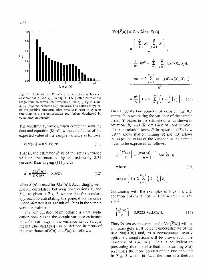
Fig. 2. Plots of the Pj values for correlations between observations X i and Xi . j in Fig. 1. The plotted correlations range from the correlation for values X~ and X~+ 1 (P1) to X~ and X, + 20 (P20) and decrease as j increases. The pattern is typical of the positive autocorrelation structures seen in systems returning to a pre-perturbation equilibrium dominated by covariance stationarity.

The resulting Pj values, when combined with the data and equation (8), allow the calculation of the expected value of the sample variance as follows:

E[S2(rt)] = 0 . 9 1 6 6 (3 "2. (11)

That is, the estimator S2(n) of the series variance will underestimate o 2 by approximately 8.34 percent. Rearranging (11) yields

02 E[S2(n)] 0.0924 (12) - 0.9166 -

when S2(n) is used for E[S2(n)]. Accordingly, with known correlation between observations X, and X t + ~ as given in Fig. 2, we see that the standard approach to calculating the population variance underestimates it as a result of a bias in the sample variance estimator.

The next question of importance is what impli- cation does bias in the sample variance estimator hold for estimates of the variance in the sample mean? The Var[X(_n)] can be defined in terms of the covariance ofX(n) andlg(n) as follows:

Var[X-(n)] = Cov[37(n), X(n)]

i n n xj] E x . E i=1 j = l

n

1 /'/ n = 7 [no + Z Z Cov(Xi, xj)],

i = t j = l

no 2 + 2 n - 1 Z

j = l (n - j)Cov(X1, Xl +2)

/7, 2

-- 1 + 2 Z 1 J j = 1 - - n Pj " (13)

This suggests two sources of error in the IID approach to estimating the variance of the sample mean: (i) biases in the estimate of o 2 as shown in equation (8), and (ii) omission of consideration of the correlation terms Pj in equation (13). Law (1977) shows that combining (8) and (13) allows the expected value of the variance of the sample mean to be expressed as follows:

E,[S2(n)] - n J (n/~n___))- 1 Var[X(n)],

where (14)

+ n221"7" j p ,] j = l

Continuing with the examples of Figs 1 and 2, equation (14) with a(n) = 1.0834 and n = 159 yields

[ ~ ] = 0.9225 Var[.~(n)]. (15)

Thus S:(n)/n as an estimator for Var[~:(n)] will be approximately an 8 percent underestimate of the true Var[X(n)] and, as a consequence, overly optimistic conclusions will be drawn about the closeness of X(n) to bt. This is equivalent to presuming that the distribution describing X(n) resembles the more pointed of the two depicted in Fig. 3 when, in fact, the true distribution

18

14

1 Actual

lO f(X) Distribution a f o ~

Estimated Distribution for X(n)

!a 0.53 0.~]8 0.zk3 0.z[8 0.53 0.'58 0.'63 0.6a 0.73 x

Fig. 3. Depicts the IID distribution for ~'(n) presumed as a result of estimating Var[~'(n)] under the assumption that all the Pj values equalled zero, and the actual distribution for X(n) when consideration of the Pj values is included. Note the false confidence about the precision of the X'(n) estimate resulting when the sample variance and Pj sources of bias are omitted from the estimate Var[X(n)].

describing X(n) is the lower, more leptokurtic, of the two distributions depicted.

4. Detecting significant correlation

The above analysis is predicated on Pj > 0. As to whether the Pj will tend to be greater than, or less than, zero, one can only speculate. Some results, however, from the study of other systems are available. Daley (1968), in a comprehensive study of queuing systems, demonstrated that the Pj values tend toward being greater than zero. Law & Kelton (1991), in discussing sequentially depen- dent models, confirm Daley's results. Accordingly, one might expect biological processes representing the end product of successive, sequential events to have similarly structured Pj results. Examples would include: recruitment, bio-concentration of toxicant residues in predator species, and post- perturbation population abundance measures. If, however, the Pj are less then zero, then S2(n)/n will overestimate Var[X(n)] and overly pessimistic conclusions will be drawn about the closeness of X(n) to g.

When the correlations Pj are mild, one may, in effect, ignore them and assume:

S~(n) ] X(n) - N [ O, ~ . (16)

201

Equation (16) allows the legitimate application of standard IID statistical procedures for testing, and inferring, significant differences in means and variances. To that end, the work of Bartlett (1946) is important. Bartlett showed that, if no correla- tion exists between observations more than k steps apart (Pj = 0 for j > k), the variances of the Pj can be approximated by

k V a r ( P j ) - - ~ l ( l + 2 ~ P ~ ) f o r j > k . (17)

rt j = l

In the special case of no correlation, (17) reduces to

Var(P~) ~ 1 f o r j > 0 (18) n

Furthermore, for large n and Pj = 0, the estimates of Pj will be approximately normal. This implies a means of testing the significance of the estimated Pj values under the null hypothesis:

H0: Pj = 0 f o r j = 1, 2 . . . . . n - 1 .

The test is completed by estimating the Pj values and their standard errors (n) 1/2 and rejecting H 0 at significance level c~ = 0.05 if

IPjl(n)m> 1.96 for j = 1, 2 . . . . . n - 1. (19)

Since one will examine a large number of Pj simultaneously, with c~ = 0.05, there is a signifi- cant likelihood of finding at least one Pj outside the bounds of_+ 1.96(n) 1/2. For 10, 20, and 30 such correlations, this probability is given by the expression 1 - (1 - cQ n = 0.40, 0.64, and 0.79, respectively. The results suggest that single exceptions to the test rule should be ignored. The overall approach, however, provides a convenient means of testing whether the observed Pj are, in fact,significant enough to confound estimates of Var[X(n)] and subsequent statistical testing and inference procedures.

5. Discussion

In the case of Pj > 0, the consequences for statis- tical testing and inference include:

202

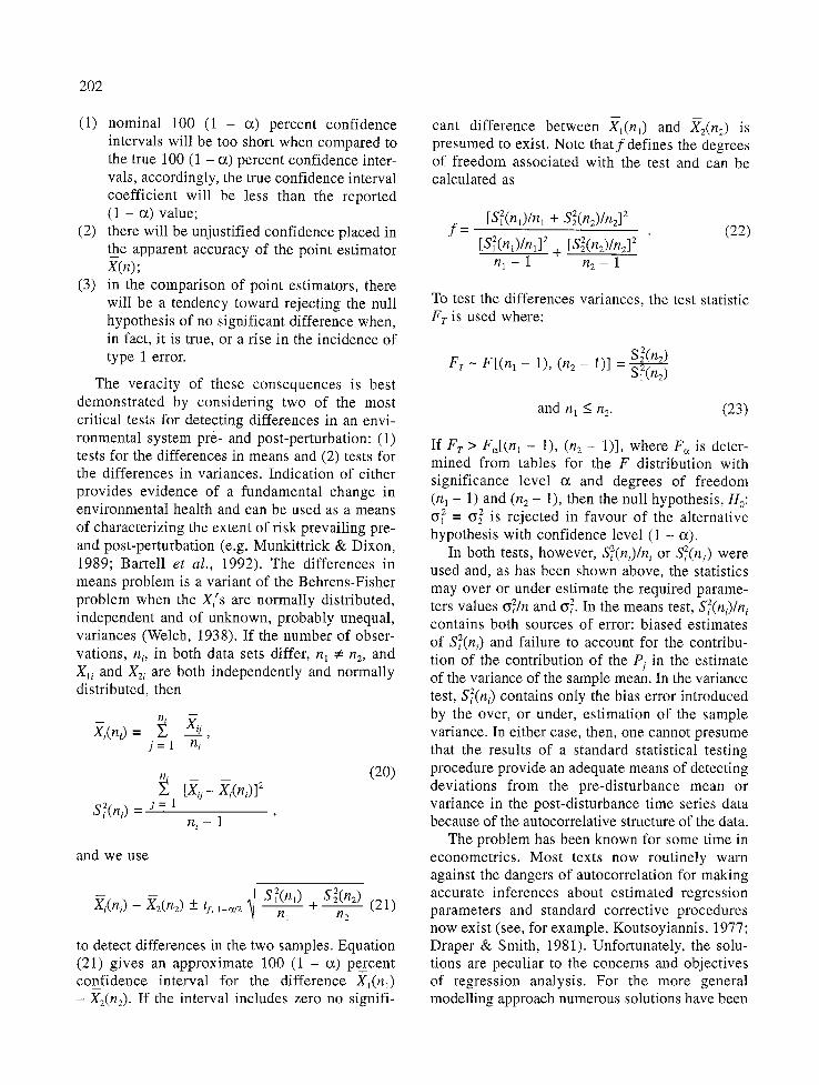
(1) nominal 100 (1 - (z) percent confidence intervals will be too short when compared to the true 100 (1 - c~) percent confidence inter- vals, accordingly, the true confidence interval coefficient will be less than the reported ( 1 - ~) value;

(2) there will be unjustified confidence placed in the apparent accuracy of the point estimator X(n);

(3) in the comparison of point estimators, there will be a tendency toward rejecting the null hypothesis of no significant difference when, in fact, it is true, or a rise in the incidence of type 1 error.

The veracity of these consequences is best demonstrated by considering two of the most critical tests for detecting differences in an envi- ronmental system pre- and post-perturbation: (1) tests for the differences in means and (2) tests for the differences in variances. Indication of either provides evidence of a fundamental change in environmental health and can be used as a means of characterizing the extent of risk prevailing pre- and post-perturbation (e.g. Munkittrick & Dixon, 1989; Bartell et al., 1992). The differences in means problem is a variant of the Behrens-Fisher problem when the Xi's are normally distributed, independent and of unknown, probably unequal, variances (Welch, 1938). If the number of obser- vations, n~, in both data sets differ, nl ~ rt2, and X~i and X2~ are both independently and normally distributed, then

j = 1 ni

S ~ ( n i ) _ j = 1 ng- 1

(20)

and we use

~ S2(nO S~(n2) (21) Xi(ni) - X2(n2) + tl, 1-~/2 nl + n2

to detect differences in the two samples. Equation (21) gives an approximate 100 (1 - c~) percent confidence interval for the difference Xl(nl) - X2(n2). If the interval includes zero no signifi-

cant difference b e t w e e n .eYl(nl) and X-2(n2) is presumed to exist. Note t h a t f defines the degrees of freedom associated with the test and can be calculated as

[S2(nl)/nx + S~(n2)/nz] 2 f = (22)

[S2(nl)/nl] 2 + [S~(n2)/n2] 2 n 1 - 1 n 2 - 1

To test the differences variances, the test statistic Fr is used where:

S~(n2) F r - F [ ( n 1 - 1), (n2 - 1)] - S~(n2)

and n 1 ~ n 2. (23)

If F r > F~[(nl - 1), (n2 - 1)], where Fa is deter- mined from tables for the F distribution with significance level c~ and degrees of freedom (nl - 1) and (n2 - 1), then the null hypothesis, H0: ~2 = cy2 is rejected in favour of the alternative hypothesis with confidence level (1 - (z ) .

In both tests, however, S~(ni)/n i or S~(nl) were used and, as has been shown above, the statistics may over or under estimate the required parame- ters values ~2/n and cy~. In the means test, S~(ni)/ni contains both sources of error: biased estimates of S~(ni) and failure to account for the contribu- tion of the contribution of the Pj in the estimate of the variance of the sample mean. In the variance test, S~(n~) contains only the bias error introduced by the over, or under, estimation of the sample variance. In either case, then, one cannot presume that the results of a standard statistical testing procedure provide an adequate means of detecting deviations from the pre-disturbance mean or variance in the post-disturbance time series data because of the autocorrelative structure of the data.

The problem has been known for some time in econometrics. Most texts now routinely warn against the dangers of autocorrelation for making accurate inferences about estimated regression parameters and standard corrective procedures now exist (see, for example, Koutsoyiannis, 1977; Draper & Smith, 1981). Unfortunately, the solu- tions are peculiar to the concerns and objectives of regression analysis. For the more general modelling approach numerous solutions have been

proposed (see, for example, Welch, 1983; Schruben, 1983; Law & Kelton, 1984; Ripley, 1987). The available corrective mechanisms, however, tend to demand large amounts of data. Batching, the most popular approach, reduces the available data series from n observations to m averaged observations of size ~, where m < n and

is chosen such that the P; between all observa- tions are zero. This, for ecological field data, where observations are often obtained at great cost or are scarce, effectively increases the resulting confidence intervals by reducing the number of observations used in their calculation. In a mod- elling analysis, this poses no problem as the modeller may compensate for the loss of obser- vations by increasing model run time. For time based field data no obvious compensating mechanism exists which, in turn, poses serious problems for the detection of changes in the envi- ronment resulting from either single or cumulative perturbations.

In the case of single perturbations, appropriate testing and detection of environmental change in the time domain requires an assessment of the autocorrelative structure, the P; values, in the post- perturbation series before the completion of statistical testing. Only then can the analyst be certain of the accuracy of the inferences made about the existence, or non-existence, of statisti- cally significant differences. In the case of cumu- lative perturbations the task is more difficult. Unless it is clear that the system under study has had sufficient time to re-establish equilibrium such that the P; values equal zero, the analysis of differences pre- and post-perturbation requires that the autocorrelative structure in both the pre- and post-perturbation data sets be assessed. Again, it is the only means the analyst has of ensuring the accuracy of the sample variance and variance of the sample mean estimates so critical to the completion of statistical hypothesis testing.

6. Conclusion

The problem of detection in environmental health assessment inevitably involves consideration of time. The comparison of an environment pre- and post-perturbation, when coupled with concerns about natural variability in the environment,

203

requires pre- and post-perturbation data sets for the effective comparison and detection of signifi- cant differences. Time, however, requires that the analysis explicitly considers the interrelationship that may exist between the sequential observa- tions. If the property of covariance stationarity is violated, the standard statistical approaches to calculating sample variance and variance of the sample mean produce biased estimates of the true population parameters. As the estimates are used in statistical hypothesis testing approaches, the approaches can no longer be considered as accurate inferential guides to environmental health or risk assessment. To the extent that correlations between adjacent observations are positive, the standard statistical formulae for the sample mean and variance of the sample mean underestimate the true population parameters. Under such con- ditions the standard hypothesis tests tend to reject a correct null hypothesis with a probability that is greater than the chosen level of significance. In other words, the testing procedure becomes invalid and errs in the direction of finding too much significance. Accordingly, before tests of the differences between observed means and variances based on time dependent data are used, it is recommended that the autocorrelative structure of the data be examined with Bartlett's test proce- dure. In the event of no statistically significant Pj values being found, classical statistical hypothesis testing procedures may be routinely used. In the event of statistically significant P; values being found, the corrective formulae developed by Anderson (1971), equation (8), and Law (1977), equation (14), can be used to adjust the estimated sample variance and variance of the sample mean estimates before using them in statistical hypoth- esis testing. Only then can appropriate and scien- tifically defensible methods for environmental health assessment be developed and confidently employed by environmental decision makers and regulators.

Acknowledgements

The author wishes to acknowledge the support and encouragement of Dr D. G. Dixon, those in his lab, and the referees for suggestions that have improved the manuscript.

204

References

Abraham, B. & J. Ledolter, 1983. Statistical Methods for Forecasting. John Wiley & Sons, New York, 445 pp.

Anderson, T. W., 1971. The Statistical Analysis of Time Series. John Wiley & Sons, New York, 704 pp.

Barnthouse, L. W., 1992. The role of models in ecological risk assessment: a 1990's perspective. Environ. Toxicol. Chem. 11: 1751-1760.

Bartell, S. M., R. H. Gardner & R. V. O'Neill, 1992. Ecological Risk Estimation. Lewis Publishers, Chelsea, 252

PP. Bartlett, M. S., 1946. On the theoretical specification of

sampling properties of autocorrelated time series. J. Roy. Statist. Soc. Series B, 8: 27-41.

Box, G. E. P. & G. M. Jenkins, 1976. Time Series Analysis." Forecasting and Control, 2nd edition. Holden-Day, San Francisco, 575 pp.

Daley, D. J., 1968. The serial correlation coefficients of waiting times in a stationary single server queue. J. Austral. Mathem. Soc. 8: 683-699.

Draper, N. R. & H. Smith, 1981. Applied Regression Analysis, 2nd edition. John Wiley & Sons, New York, 709 pp.

Emlen, J. M., 1989. Terrestrial population models for ecological risk assessment: a state-of-the-art review. Environ. Toxicol. Chem. 8: 831-842.

Ferson, S., L. Ginzburg & A. Silvers, 1989. Extreme event risk analysis for age-structured populations. Ecolog. Modelling 47: 175-187.

Hogg, R. V. & A. T. Craig, 1978. Introduction to Mathematical Statistics, 4th edition. Macmillan, New

York, 438 pp. Koutsoyiannis, A., 1977. Theory of Econometrics, 2nd edition.

Macmillan, London, 639 pp. Law, A. M., 1977. Confidence intervals in discrete event

simulation: a comparison of replication and batch means. Naval Res. Logistics Quart. 23: 667-678.

Law, A. M. & W. D. Kelton, 1984. Confidence intervals for steady-state simulations, I: a survey of fixed sample size procedures. Operation Res. 32: 1221-1239.

Law, A. M. & W. D. Kelton, 1991. Simulation & Modeling Analysis, 2nd edition. McGraw-Hill, New York, 759 pp.

Minns, C. K., 1992. Use of models for integrated assessment of ecosystem health. J. Aquat. Ecosyst. Health 1: 109- 118.

Munkittrick, K. R. & D. G. Dixon, 1989. Use of white sucker (Catostomus commersoni) populations to assess the health of aquatic ecosystems exposed to low-level contaminant stress. Can. J. Fish. Aquat. Sci. 46: 1455-1462.

Ripley, B. D., 1987. Stochastic Simulation. John Wiley & Sons, New York, 237 pp.

Ross, S. M., 1985. Introduction to Probability Models, 3rd edition. Academic Press, New York, 502 pp.

Schruben, L. W., 1983. Confidence interval estimation using standardized time series. Operations Res. 31: 1090-1108.

Welch, B. L., 1938. The significance of the difference between two means when the population variances are unequal. Biometrika 25: 350-362.

Welch, P. D., 1983. The statistical analysis of simulation results. In: S. S. Lavenberg (ed.), The Computer Performance Modeling Handbook. pp. 268-328. Academic Press, New York.