Embed Size (px)
Citation preview
The state of female autonomy in India: astochastic dominance approach
Kausik Chaudhuri Gaston Yalonetzky
Leeds University Business School
November 2013

Table of contents
Introduction
Methodology
Data and estimation choices
Results
Concluding remarks

Introduction
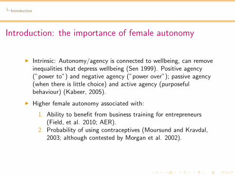
Introduction: the importance of female autonomy
I Intrinsic: Autonomy/agency is connected to wellbeing, can removeinequalities that depress wellbeing (Sen 1999).
Positive agency(”power to”) and negative agency (”power over”); passive agency(when there is little choice) and active agency (purposefulbehaviour) (Kabeer, 2005).
I Higher female autonomy associated with:
1. Ability to benefit from business training for entrepreneurs(Field, et al. 2010; AER).
2. Probability of using contraceptives (Moursund and Kravdal,2003; although contested by Morgan et al. 2002).
3. Prenatal care, delivery and postnatal care (Mistry et al. 2009).

Introduction
Introduction: the importance of female autonomy
I Intrinsic: Autonomy/agency is connected to wellbeing, can removeinequalities that depress wellbeing (Sen 1999). Positive agency(”power to”) and negative agency (”power over”); passive agency(when there is little choice) and active agency (purposefulbehaviour) (Kabeer, 2005).
I Higher female autonomy associated with:
1. Ability to benefit from business training for entrepreneurs(Field, et al. 2010; AER).
2. Probability of using contraceptives (Moursund and Kravdal,2003; although contested by Morgan et al. 2002).
3. Prenatal care, delivery and postnatal care (Mistry et al. 2009).
Introduction
Introduction: female autonomy in India
I Long history of many studies on India (also Bangladesh, Pakistanand other major Asian nations), e.g. Dyson and Moore (1983).
I Main themes: Measurement, causes (”determinants”) andconsequences/impacts; mismatch in perceptions between husbandand wife.
I Typical correlates:
1. Kinship systems (posited by Dyson and Moore).2. Woman’s earnings, family income (in Bangladesh, Anderson
and Eswaran 2008); dowry, goods owned (Jejeeboy and Sathar,2001).
3. Wife and husband education (Anderson and Eswaran 2008;Jejeeboy and Sathar, 2001).
4. Co-residing mother-in-law (AE, 2008; JS 2001).5. Religion and region (Jejeeboy and Sathar, 2001).
Introduction
Introduction: female autonomy in India
I Long history of many studies on India (also Bangladesh, Pakistanand other major Asian nations), e.g. Dyson and Moore (1983).
I Main themes: Measurement, causes (”determinants”) andconsequences/impacts; mismatch in perceptions between husbandand wife.
I Typical correlates:
1. Kinship systems (posited by Dyson and Moore).
2. Woman’s earnings, family income (in Bangladesh, Andersonand Eswaran 2008); dowry, goods owned (Jejeeboy and Sathar,2001).
3. Wife and husband education (Anderson and Eswaran 2008;Jejeeboy and Sathar, 2001).
4. Co-residing mother-in-law (AE, 2008; JS 2001).5. Religion and region (Jejeeboy and Sathar, 2001).

Introduction
Introduction: female autonomy in India
I Long history of many studies on India (also Bangladesh, Pakistanand other major Asian nations), e.g. Dyson and Moore (1983).
I Main themes: Measurement, causes (”determinants”) andconsequences/impacts; mismatch in perceptions between husbandand wife.
I Typical correlates:
1. Kinship systems (posited by Dyson and Moore).2. Woman’s earnings, family income (in Bangladesh, Anderson
and Eswaran 2008); dowry, goods owned (Jejeeboy and Sathar,2001).
3. Wife and husband education (Anderson and Eswaran 2008;Jejeeboy and Sathar, 2001).
4. Co-residing mother-in-law (AE, 2008; JS 2001).5. Religion and region (Jejeeboy and Sathar, 2001).

Introduction
Introduction: female autonomy in India
I Long history of many studies on India (also Bangladesh, Pakistanand other major Asian nations), e.g. Dyson and Moore (1983).
I Main themes: Measurement, causes (”determinants”) andconsequences/impacts; mismatch in perceptions between husbandand wife.
I Typical correlates:
1. Kinship systems (posited by Dyson and Moore).2. Woman’s earnings, family income (in Bangladesh, Anderson
and Eswaran 2008); dowry, goods owned (Jejeeboy and Sathar,2001).
3. Wife and husband education (Anderson and Eswaran 2008;Jejeeboy and Sathar, 2001).
4. Co-residing mother-in-law (AE, 2008; JS 2001).
5. Religion and region (Jejeeboy and Sathar, 2001).

Introduction
Introduction: female autonomy in India
I Long history of many studies on India (also Bangladesh, Pakistanand other major Asian nations), e.g. Dyson and Moore (1983).
I Main themes: Measurement, causes (”determinants”) andconsequences/impacts; mismatch in perceptions between husbandand wife.
I Typical correlates:
1. Kinship systems (posited by Dyson and Moore).2. Woman’s earnings, family income (in Bangladesh, Anderson
and Eswaran 2008); dowry, goods owned (Jejeeboy and Sathar,2001).
3. Wife and husband education (Anderson and Eswaran 2008;Jejeeboy and Sathar, 2001).
4. Co-residing mother-in-law (AE, 2008; JS 2001).5. Religion and region (Jejeeboy and Sathar, 2001).

Introduction
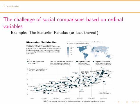
The challenge of social comparisons based on ordinalvariables
I We would like to compare levels of female autonomy acrossdifferent Indian states, and our autonomy variables are ordinal.
I Allison and Foster (2004) noted that comparisons of averagesbased on ordinal variables are not very reliable since theydepend on arbitrary scales.
I Despite this warning, averages from ordinal variables are stillheavily used in many literatures.

Introduction
The challenge of social comparisons based on ordinalvariables
I We would like to compare levels of female autonomy acrossdifferent Indian states, and our autonomy variables are ordinal.
I Allison and Foster (2004) noted that comparisons of averagesbased on ordinal variables are not very reliable since theydepend on arbitrary scales.
I Despite this warning, averages from ordinal variables are stillheavily used in many literatures.

Introduction
The challenge of social comparisons based on ordinalvariables
Example: The Easterlin Paradox (or lack thereof)
Introduction
The challenge of social comparisons based on ordinalvariables
Example: The Easterlin Paradox (or lack thereof)
Introduction
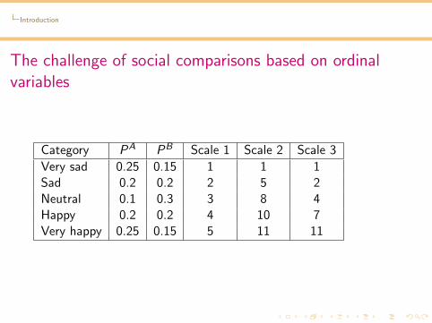
The challenge of social comparisons based on ordinalvariables
Category PA PB Scale 1 Scale 2 Scale 3
Very sad 0.25 0.15 1 1 1Sad 0.2 0.2 2 5 2Neutral 0.1 0.3 3 8 4Happy 0.2 0.2 4 10 7Very happy 0.25 0.15 5 11 11

Introduction
The challenge of social comparisons based on ordinalvariables
Which country has a higher average happiness? A or B?
Scale µA µB
1 3 32 6.8 7.23 5.2 4.8

Introduction
The challenge of social comparisons based on ordinalvariables
Which country has a higher average happiness? A or B?
Scale µA µB
1 3 32 6.8 7.23 5.2 4.8
Introduction
The challenge of social comparisons based on ordinalvariables
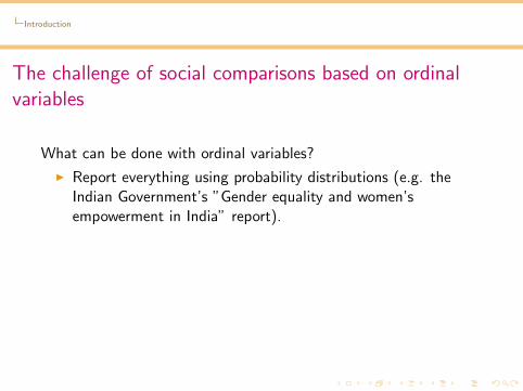
What can be done with ordinal variables?
I Report everything using probability distributions (e.g. theIndian Government’s ”Gender equality and women’sempowerment in India” report).
I Latent variable models (e.g. ordered probit; MIMIC, SEM,etc.).
I A counting approach.
I Stochastic dominance and related non-parametricdistributional analysis tools.
Introduction
The challenge of social comparisons based on ordinalvariables
What can be done with ordinal variables?
I Report everything using probability distributions (e.g. theIndian Government’s ”Gender equality and women’sempowerment in India” report).
I Latent variable models (e.g. ordered probit; MIMIC, SEM,etc.).
I A counting approach.
I Stochastic dominance and related non-parametricdistributional analysis tools.
Introduction
Introduction: This paper’s contribution
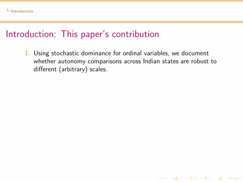
1. Using stochastic dominance for ordinal variables, we documentwhether autonomy comparisons across Indian states are robust todifferent (arbitrary) scales.
2. When the dominance conditions hold, the ensuing robust orderinghas an interpretation in terms of preferences over lotteries based onindividual ”utility” functions.
3. We also show how to rank the dominance conditions in terms of thedifferences in social welfare that they entail.
4. We find that Southern and North-Easter states tend to dominateNorthern states. But there are important exceptions and resultsdepend on the autonomy aspect.
5. The strongest welfare differences usually involve North-Easternstates dominating Northern states.

Introduction
Introduction: This paper’s contribution
1. Using stochastic dominance for ordinal variables, we documentwhether autonomy comparisons across Indian states are robust todifferent (arbitrary) scales.
2. When the dominance conditions hold, the ensuing robust orderinghas an interpretation in terms of preferences over lotteries based onindividual ”utility” functions.
3. We also show how to rank the dominance conditions in terms of thedifferences in social welfare that they entail.
4. We find that Southern and North-Easter states tend to dominateNorthern states.
But there are important exceptions and resultsdepend on the autonomy aspect.
5. The strongest welfare differences usually involve North-Easternstates dominating Northern states.
Introduction
Introduction: This paper’s contribution
1. Using stochastic dominance for ordinal variables, we documentwhether autonomy comparisons across Indian states are robust todifferent (arbitrary) scales.
2. When the dominance conditions hold, the ensuing robust orderinghas an interpretation in terms of preferences over lotteries based onindividual ”utility” functions.
3. We also show how to rank the dominance conditions in terms of thedifferences in social welfare that they entail.
4. We find that Southern and North-Easter states tend to dominateNorthern states. But there are important exceptions and resultsdepend on the autonomy aspect.
5. The strongest welfare differences usually involve North-Easternstates dominating Northern states.

Introduction
The organization of the rest of this presentation
I Methodology.
I Data.
I Results.
I Concluding remarks.

Introduction
The organization of the rest of this presentation
I Methodology.
I Data.
I Results.
I Concluding remarks.

Introduction
The organization of the rest of this presentation
I Methodology.
I Data.
I Results.
I Concluding remarks.

Introduction
The organization of the rest of this presentation
I Methodology.
I Data.
I Results.
I Concluding remarks.

Methodology
Notation and preliminaries
Let X be an ordinal variable with S categories, such that:x1 ≤ x2 ≤ ... ≤ xS .
The distribution of X in a society is given by:P : [p(1), p(2), ..., p(S)], where: p(i) ≡ Pr[X = xi ]. Likewise thecumulative distribution is: F : [F (1),F (2), ...,F (S)], where:F (i) =
∑ij=1 p(j).
A person with X = xi enjoys utility U(i). Society’s expected oraverage welfare is: W =
∑Si=1 p(i)U(i).
For society A we add subscripts to the formulas.

Methodology
Notation and preliminaries
Let X be an ordinal variable with S categories, such that:x1 ≤ x2 ≤ ... ≤ xS .
The distribution of X in a society is given by:P : [p(1), p(2), ..., p(S)], where: p(i) ≡ Pr[X = xi ].
Likewise thecumulative distribution is: F : [F (1),F (2), ...,F (S)], where:F (i) =
∑ij=1 p(j).
A person with X = xi enjoys utility U(i). Society’s expected oraverage welfare is: W =
∑Si=1 p(i)U(i).
For society A we add subscripts to the formulas.
Methodology
Notation and preliminaries
Let X be an ordinal variable with S categories, such that:x1 ≤ x2 ≤ ... ≤ xS .
The distribution of X in a society is given by:P : [p(1), p(2), ..., p(S)], where: p(i) ≡ Pr[X = xi ]. Likewise thecumulative distribution is: F : [F (1),F (2), ...,F (S)], where:F (i) =
∑ij=1 p(j).
A person with X = xi enjoys utility U(i). Society’s expected oraverage welfare is: W =
∑Si=1 p(i)U(i).
For society A we add subscripts to the formulas.

Methodology
Notation and preliminaries
Let X be an ordinal variable with S categories, such that:x1 ≤ x2 ≤ ... ≤ xS .
The distribution of X in a society is given by:P : [p(1), p(2), ..., p(S)], where: p(i) ≡ Pr[X = xi ]. Likewise thecumulative distribution is: F : [F (1),F (2), ...,F (S)], where:F (i) =
∑ij=1 p(j).
A person with X = xi enjoys utility U(i). Society’s expected oraverage welfare is: W =
∑Si=1 p(i)U(i).
For society A we add subscripts to the formulas.
Methodology
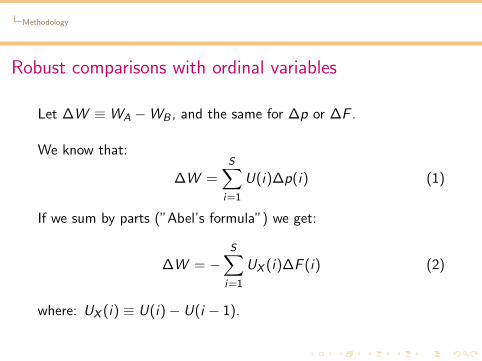
Robust comparisons with ordinal variables
Let ∆W ≡WA −WB , and the same for ∆p or ∆F .
We know that:
∆W =S∑
i=1
U(i)∆p(i) (1)
If we sum by parts (”Abel’s formula”) we get:
∆W = −S∑
i=1
UX (i)∆F (i) (2)
where: UX (i) ≡ U(i)− U(i − 1).

Methodology
Robust comparisons with ordinal variables
Let ∆W ≡WA −WB , and the same for ∆p or ∆F .
We know that:
∆W =S∑
i=1
U(i)∆p(i) (1)
If we sum by parts (”Abel’s formula”) we get:
∆W = −S∑
i=1
UX (i)∆F (i) (2)
where: UX (i) ≡ U(i)− U(i − 1).
Methodology
Robust comparisons with ordinal variables
Let ∆W ≡WA −WB , and the same for ∆p or ∆F .
We know that:
∆W =S∑
i=1
U(i)∆p(i) (1)
If we sum by parts (”Abel’s formula”) we get:
∆W = −S∑
i=1
UX (i)∆F (i) (2)
where: UX (i) ≡ U(i)− U(i − 1).

Methodology
Robust comparisons with ordinal variables
Now with equation 2 (∆W = −∑S
i=1 UX (i)∆F (i)) we derive thefollowing first-order dominance condition:
First-order dominance condition
∆W > 0 ∀UX > 0↔ ∆F (i) ≤ 0 ∀i ∈ [1,S ] ∧ ∃j |∆F (j) < 0

Methodology
Robust comparisons with ordinal variables
Summing equation 2 by parts yields also a second-order dominancecondition which is relevant for concave utility functions and/orconcave (arbitrary) scales:
Second-order dominance condition
∆W ≥ 0 ∀UX > 0 ∧ UXX ≤ 0 ↔ ∆G (i) ≤ 0 ∀i ∈ [1,S ] ∧∃j |∆G (j) < 0
where: UXX (i) = UX (i)− UX (i − 1) and G (i) =∑i
j=1 F (j).
Methodology
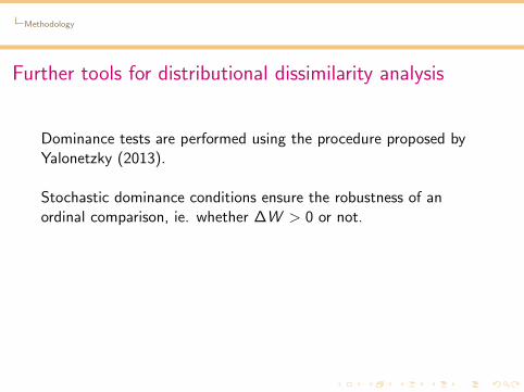
Further tools for distributional dissimilarity analysis
Dominance tests are performed using the procedure proposed byYalonetzky (2013).
Stochastic dominance conditions ensure the robustness of anordinal comparison, ie. whether ∆W > 0 or not. However they aresilent as to the magnitude of the difference.
Can we do better than this? Yes: Two additional distributionalconditions are informative of the quantitative differences betweentwo (or more) comparison pairs.
Methodology
Further tools for distributional dissimilarity analysis
Dominance tests are performed using the procedure proposed byYalonetzky (2013).
Stochastic dominance conditions ensure the robustness of anordinal comparison, ie. whether ∆W > 0 or not.
However they aresilent as to the magnitude of the difference.
Can we do better than this? Yes: Two additional distributionalconditions are informative of the quantitative differences betweentwo (or more) comparison pairs.

Methodology
Further tools for distributional dissimilarity analysis
Dominance tests are performed using the procedure proposed byYalonetzky (2013).
Stochastic dominance conditions ensure the robustness of anordinal comparison, ie. whether ∆W > 0 or not. However they aresilent as to the magnitude of the difference.
Can we do better than this? Yes: Two additional distributionalconditions are informative of the quantitative differences betweentwo (or more) comparison pairs.

Methodology
Further tools for distributional dissimilarity analysis
Dominance tests are performed using the procedure proposed byYalonetzky (2013).
Stochastic dominance conditions ensure the robustness of anordinal comparison, ie. whether ∆W > 0 or not. However they aresilent as to the magnitude of the difference.
Can we do better than this?
Yes: Two additional distributionalconditions are informative of the quantitative differences betweentwo (or more) comparison pairs.

Methodology
Further tools for distributional dissimilarity analysis
Dominance tests are performed using the procedure proposed byYalonetzky (2013).
Stochastic dominance conditions ensure the robustness of anordinal comparison, ie. whether ∆W > 0 or not. However they aresilent as to the magnitude of the difference.
Can we do better than this? Yes: Two additional distributionalconditions are informative of the quantitative differences betweentwo (or more) comparison pairs.

Methodology
Intensity of the first-order dominance condition: the strongcase
Let ∆WA−B = WA −WB and ∆WC−D = WC −WD and assumethat A and C dominate B and D respectively.
Using equation 2 itis easy to prove the following:
Strong dominance intensity
∆WA−B > ∆WC−D ∀UX > 0 ↔ ∆FA−B(i) ≤ ∆FC−D(i) ∀i ∈[1, S ] ∧ ∃j |∆FA−B(j) < ∆FC−D(j)
This condition requires comparing pairs of pairs, i.e. pairs of ∆Ffor each category and each comparison pair (e.g. A-B versus C-D).Since it is too cumbersome for our purposes, we do not use it inthe paper (as we have hundreds of comparisons), but it is used inChaudhuri, Gradin and Yalonetzky (2012).

Methodology
Intensity of the first-order dominance condition: the strongcase
Let ∆WA−B = WA −WB and ∆WC−D = WC −WD and assumethat A and C dominate B and D respectively. Using equation 2 itis easy to prove the following:
Strong dominance intensity
∆WA−B > ∆WC−D ∀UX > 0 ↔ ∆FA−B(i) ≤ ∆FC−D(i) ∀i ∈[1, S ] ∧ ∃j |∆FA−B(j) < ∆FC−D(j)
This condition requires comparing pairs of pairs, i.e. pairs of ∆Ffor each category and each comparison pair (e.g. A-B versus C-D).
Since it is too cumbersome for our purposes, we do not use it inthe paper (as we have hundreds of comparisons), but it is used inChaudhuri, Gradin and Yalonetzky (2012).

Methodology
Intensity of the first-order dominance condition: the strongcase
Let ∆WA−B = WA −WB and ∆WC−D = WC −WD and assumethat A and C dominate B and D respectively. Using equation 2 itis easy to prove the following:
Strong dominance intensity
∆WA−B > ∆WC−D ∀UX > 0 ↔ ∆FA−B(i) ≤ ∆FC−D(i) ∀i ∈[1, S ] ∧ ∃j |∆FA−B(j) < ∆FC−D(j)
This condition requires comparing pairs of pairs, i.e. pairs of ∆Ffor each category and each comparison pair (e.g. A-B versus C-D).Since it is too cumbersome for our purposes, we do not use it inthe paper (as we have hundreds of comparisons), but it is used inChaudhuri, Gradin and Yalonetzky (2012).
Methodology
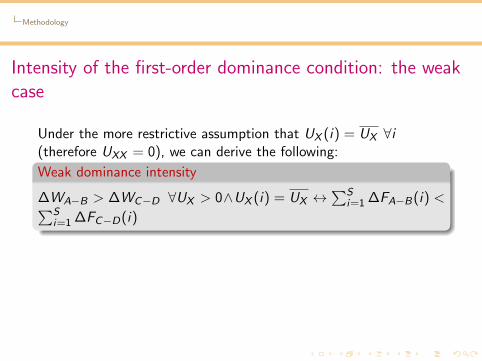
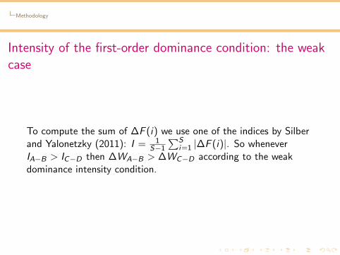
Intensity of the first-order dominance condition: the weakcase
Under the more restrictive assumption that UX (i) = UX ∀i(therefore UXX = 0), we can derive the following:
Weak dominance intensity
∆WA−B > ∆WC−D ∀UX > 0∧UX (i) = UX ↔∑S
i=1 ∆FA−B(i) <∑Si=1 ∆FC−D(i)
This condition only requires comparing the sums of ∆F (i) acrosscategories for each comparison pair. In this paper we use thiscondition in order to rank the dominance relationships in terms oftheir degree of weak intensity.

Methodology
Intensity of the first-order dominance condition: the weakcase
Under the more restrictive assumption that UX (i) = UX ∀i(therefore UXX = 0), we can derive the following:
Weak dominance intensity
∆WA−B > ∆WC−D ∀UX > 0∧UX (i) = UX ↔∑S
i=1 ∆FA−B(i) <∑Si=1 ∆FC−D(i)
This condition only requires comparing the sums of ∆F (i) acrosscategories for each comparison pair.
In this paper we use thiscondition in order to rank the dominance relationships in terms oftheir degree of weak intensity.

Methodology
Intensity of the first-order dominance condition: the weakcase
Under the more restrictive assumption that UX (i) = UX ∀i(therefore UXX = 0), we can derive the following:
Weak dominance intensity
∆WA−B > ∆WC−D ∀UX > 0∧UX (i) = UX ↔∑S
i=1 ∆FA−B(i) <∑Si=1 ∆FC−D(i)
This condition only requires comparing the sums of ∆F (i) acrosscategories for each comparison pair. In this paper we use thiscondition in order to rank the dominance relationships in terms oftheir degree of weak intensity.
Methodology
Intensity of the first-order dominance condition: the weakcase
To compute the sum of ∆F (i) we use one of the indices by Silberand Yalonetzky (2011): I = 1
S−1
∑Si=1 |∆F (i)|. So whenever
IA−B > IC−D then ∆WA−B > ∆WC−D according to the weakdominance intensity condition.

Methodology
Intensity of the first-order dominance condition
The strong case provides a quasi-ordering within an existingquasi-ordering.
But it is fully robust.
The weak case provides an ordering within an existingquasi-ordering. However it applies to a limited range of welfarefunctions.

Methodology
Intensity of the first-order dominance condition
The strong case provides a quasi-ordering within an existingquasi-ordering.But it is fully robust.
The weak case provides an ordering within an existingquasi-ordering. However it applies to a limited range of welfarefunctions.
Methodology
Intensity of the first-order dominance condition
The strong case provides a quasi-ordering within an existingquasi-ordering.But it is fully robust.
The weak case provides an ordering within an existingquasi-ordering.
However it applies to a limited range of welfarefunctions.

Methodology
Intensity of the first-order dominance condition
The strong case provides a quasi-ordering within an existingquasi-ordering.But it is fully robust.
The weak case provides an ordering within an existingquasi-ordering. However it applies to a limited range of welfarefunctions.

Data and estimation choices
Data details
I Dataset: India’s National Family Health Survey 2005-6.
I 87588 women aged 15 to 49.
I Every Indian state has at least 1,000 observations.
I More than 90% of households headed by men.
I 29 Indian states, therefore 406 comparisons!

Data and estimation choices
Data details
I Dataset: India’s National Family Health Survey 2005-6.
I 87588 women aged 15 to 49.
I Every Indian state has at least 1,000 observations.
I More than 90% of households headed by men.
I 29 Indian states, therefore 406 comparisons!

Data and estimation choices
Data details
I Dataset: India’s National Family Health Survey 2005-6.
I 87588 women aged 15 to 49.
I Every Indian state has at least 1,000 observations.
I More than 90% of households headed by men.
I 29 Indian states, therefore 406 comparisons!

Data and estimation choices
Data details
I Dataset: India’s National Family Health Survey 2005-6.
I 87588 women aged 15 to 49.
I Every Indian state has at least 1,000 observations.
I More than 90% of households headed by men.
I 29 Indian states, therefore 406 comparisons!
Data and estimation choices
Data details
I Dataset: India’s National Family Health Survey 2005-6.
I 87588 women aged 15 to 49.
I Every Indian state has at least 1,000 observations.
I More than 90% of households headed by men.
I 29 Indian states, therefore 406 comparisons!

Data and estimation choices
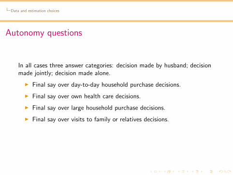
Autonomy questions
In all cases three answer categories: decision made by husband; decisionmade jointly; decision made alone.
I Final say over day-to-day household purchase decisions.
I Final say over own health care decisions.
I Final say over large household purchase decisions.
I Final say over visits to family or relatives decisions.
I Final say over spending husband’s money decisions.
Data and estimation choices
Autonomy questions
In all cases three answer categories: decision made by husband; decisionmade jointly; decision made alone.
I Final say over day-to-day household purchase decisions.
I Final say over own health care decisions.
I Final say over large household purchase decisions.
I Final say over visits to family or relatives decisions.
I Final say over spending husband’s money decisions.
Data and estimation choices
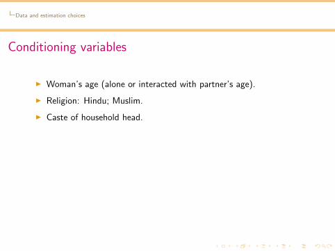
Conditioning variables
I Woman’s age (alone or interacted with partner’s age).
I Religion: Hindu; Muslim.
I Caste of household head.
I Woman’s education (if less than 3 years) interacted with partner’seducation (if more than two years).
I Urban.
I Wealth quartiles.
Overall we tried 11 conditioning specifications. But I will show you onlythe following: young women (31-); urban women; wealthiest women (inaddition to unconditioned results).

Data and estimation choices
Conditioning variables
I Woman’s age (alone or interacted with partner’s age).
I Religion: Hindu; Muslim.
I Caste of household head.
I Woman’s education (if less than 3 years) interacted with partner’seducation (if more than two years).
I Urban.
I Wealth quartiles.
Overall we tried 11 conditioning specifications. But I will show you onlythe following: young women (31-); urban women; wealthiest women (inaddition to unconditioned results).

Data and estimation choices
Conditioning variables
I Woman’s age (alone or interacted with partner’s age).
I Religion: Hindu; Muslim.
I Caste of household head.
I Woman’s education (if less than 3 years) interacted with partner’seducation (if more than two years).
I Urban.
I Wealth quartiles.
Overall we tried 11 conditioning specifications.
But I will show you onlythe following: young women (31-); urban women; wealthiest women (inaddition to unconditioned results).

Data and estimation choices
Conditioning variables
I Woman’s age (alone or interacted with partner’s age).
I Religion: Hindu; Muslim.
I Caste of household head.
I Woman’s education (if less than 3 years) interacted with partner’seducation (if more than two years).
I Urban.
I Wealth quartiles.
Overall we tried 11 conditioning specifications. But I will show you onlythe following: young women (31-); urban women; wealthiest women (inaddition to unconditioned results).

Data and estimation choices
Indian states

Results
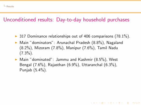
Unconditioned results: Day-to-day household purchases
I 317 Dominance relationships out of 406 comparisons (78.1%).
I Main ”dominators”: Arunachal Pradesh (8.8%), Nagaland(8.2%), Mizoram (7.8%), Manipur (7.6%), Tamil Nadu(7.3%).
I Main ”dominated”: Jammu and Kashmir (8.5%), WestBengal (7.6%), Rajasthan (6.9%), Uttaranchal (6.3%),Punjab (5.4%).
I ”Top five” relationships: AruP>JK (0.3877), Nagaland>JK(0.3805), Mizoram>JK (0.3628), Manipur>JK (0.3546),Tamil Nadu>JK (0.3514).

Results
Unconditioned results: Day-to-day household purchases
I 317 Dominance relationships out of 406 comparisons (78.1%).
I Main ”dominators”: Arunachal Pradesh (8.8%), Nagaland(8.2%), Mizoram (7.8%), Manipur (7.6%), Tamil Nadu(7.3%).
I Main ”dominated”: Jammu and Kashmir (8.5%), WestBengal (7.6%), Rajasthan (6.9%), Uttaranchal (6.3%),Punjab (5.4%).
I ”Top five” relationships: AruP>JK (0.3877), Nagaland>JK(0.3805), Mizoram>JK (0.3628), Manipur>JK (0.3546),Tamil Nadu>JK (0.3514).
Results
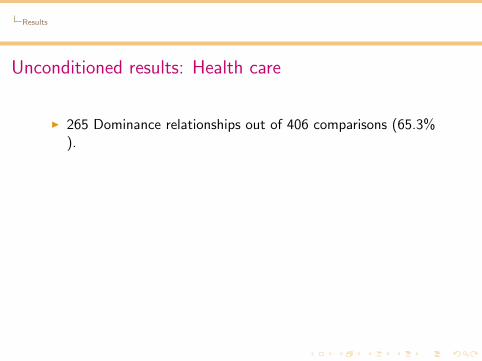
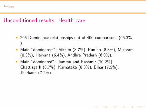
Unconditioned results: Health care
I 265 Dominance relationships out of 406 comparisons (65.3%).
I Main ”dominators”: Sikkim (8.7%), Punjab (8.3%), Mizoram(8.3%), Haryana (6.4%), Andhra Pradesh (6.0%).
I Main ”dominated”: Jammu and Kashmir (10.2%),Chattisgarh (8.7%), Karnataka (8.3%), Bihar (7.5%),Jharkand (7.2%).
I ”Top five” relationships: Mizoram>JK (0.3253), Sikkim>JK(0.3251), Punjab>JK (0.3145), Mizoram>Chatisgarh(0.2836), Sikkim>Chatisgarh (0.2834).

Results
Unconditioned results: Health care
I 265 Dominance relationships out of 406 comparisons (65.3%).
I Main ”dominators”: Sikkim (8.7%), Punjab (8.3%), Mizoram(8.3%), Haryana (6.4%), Andhra Pradesh (6.0%).
I Main ”dominated”: Jammu and Kashmir (10.2%),Chattisgarh (8.7%), Karnataka (8.3%), Bihar (7.5%),Jharkand (7.2%).
I ”Top five” relationships: Mizoram>JK (0.3253), Sikkim>JK(0.3251), Punjab>JK (0.3145), Mizoram>Chatisgarh(0.2836), Sikkim>Chatisgarh (0.2834).

Results
Unconditioned results: Large purchases
I 230 Dominance relationships out of 406 comparisons (56.7%).
I Main ”dominators”: Meghalaya (11%), Mizoram (9.6%),Nagaland (8.3%), Tamil Nadu (8.3%), Goa (8.3%).
I Main ”dominated”: Rajasthan (9.6%), Chattisgarh (8.7%),Haryana (7.4%), Punjab (6.5%), Jammu and Kashmir (6.5%).
I ”Top five” relationships: Meghalaya>Rajasthan (0.2541),Mizoram>Rajasthan (0.2333), Meghalaya>JK (0.2318),AruP>Rajasthan (0.2317), Nagaland>Rajasthan (0.2236).

Results
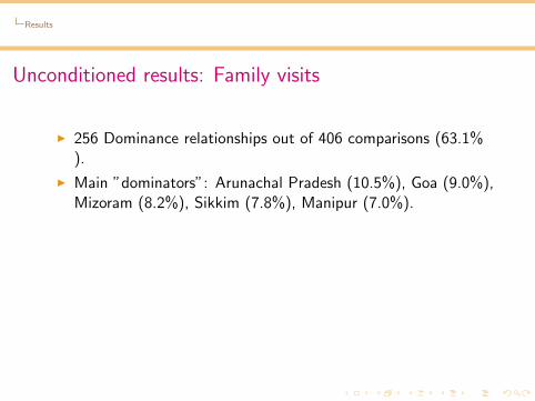
Unconditioned results: Family visits
I 256 Dominance relationships out of 406 comparisons (63.1%).
I Main ”dominators”: Arunachal Pradesh (10.5%), Goa (9.0%),Mizoram (8.2%), Sikkim (7.8%), Manipur (7.0%).
I Main ”dominated”: Jammu and Kashmir (10.2%), MadhyaPradesh (8.2%), Rajasthan (8.2%), Uttar Pradesh (7.8%),Chattisgarh (7.0%).
I ”Top five” relationships: AruP>JK (0.3542),AruP>Rajasthan (0.3378), Goa>JK (0.3148),Goa>Rajasthan (0.2984), AruP>MP (0.2906).
Results
Unconditioned results: Family visits
I 256 Dominance relationships out of 406 comparisons (63.1%).
I Main ”dominators”: Arunachal Pradesh (10.5%), Goa (9.0%),Mizoram (8.2%), Sikkim (7.8%), Manipur (7.0%).
I Main ”dominated”: Jammu and Kashmir (10.2%), MadhyaPradesh (8.2%), Rajasthan (8.2%), Uttar Pradesh (7.8%),Chattisgarh (7.0%).
I ”Top five” relationships: AruP>JK (0.3542),AruP>Rajasthan (0.3378), Goa>JK (0.3148),Goa>Rajasthan (0.2984), AruP>MP (0.2906).

Results
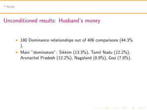
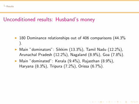
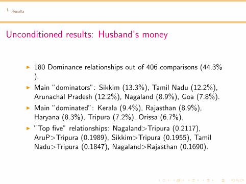
Unconditioned results: Husband’s money
I 180 Dominance relationships out of 406 comparisons (44.3%).
I Main ”dominators”: Sikkim (13.3%), Tamil Nadu (12.2%),Arunachal Pradesh (12.2%), Nagaland (8.9%), Goa (7.8%).
I Main ”dominated”: Kerala (9.4%), Rajasthan (8.9%),Haryana (8.3%), Tripura (7.2%), Orissa (6.7%).
I ”Top five” relationships: Nagaland>Tripura (0.2117),AruP>Tripura (0.1989), Sikkim>Tripura (0.1955), TamilNadu>Tripura (0.1847), Nagaland>Rajasthan (0.1690).
Results
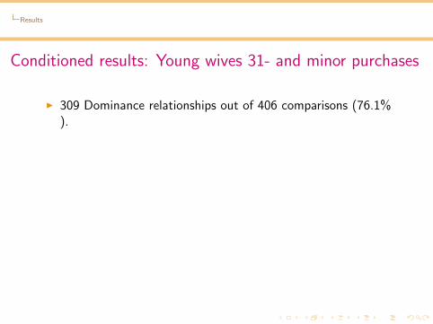
Conditioned results: Young wives 31- and minor purchases
I 309 Dominance relationships out of 406 comparisons (76.1%).
I Main ”dominators”: Arunachal Pradesh (9.1%), Nagaland(8.4%), Tamil Nadu (7.8%), Mizoram (7.8%), Manipur(7.1%).
I Main ”dominated”: Jammu and Kashmir (8.7%), Rajasthan(7.1%), Punjab (6.8%), Uttaranchal (5.8%), West Bengal(5.8%).
I ”Top five” relationships: AruP>JK (0.4665),AruP>Rajasthan (0.4299), Nagaland>JK (0.4189),AruP>Punjab (0.4018), AruP>WB (0.3991).

Results
Conditioned results: Young wives 31- and minor purchases
I 309 Dominance relationships out of 406 comparisons (76.1%).
I Main ”dominators”: Arunachal Pradesh (9.1%), Nagaland(8.4%), Tamil Nadu (7.8%), Mizoram (7.8%), Manipur(7.1%).
I Main ”dominated”: Jammu and Kashmir (8.7%), Rajasthan(7.1%), Punjab (6.8%), Uttaranchal (5.8%), West Bengal(5.8%).
I ”Top five” relationships: AruP>JK (0.4665),AruP>Rajasthan (0.4299), Nagaland>JK (0.4189),AruP>Punjab (0.4018), AruP>WB (0.3991).
Results
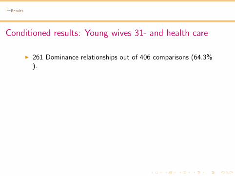
Conditioned results: Young wives 31- and health care
I 261 Dominance relationships out of 406 comparisons (64.3%).
I Main ”dominators”: Mizoram (9.6%), Sikkim (9.2%), Punjab(7.7%), Andhra Pradesh (6.1%), Tamil Nadu (5.7%), Haryana(5.7%).
I Main ”dominated”: Jammu and Kashmir (10.0%),Chattisgarh (8.8%), Karnataka (8.4%), Bihar (7.7%), MadhyaPradesh (7.3%).
I ”Top five” relationships: Mizoram> JK (0.3562), Sikkim>JK(0.3255), Mizoram>Karnataka (0.3213),Mizoram>Chatisgarh (0.3213), Mizoram>Bihar (0.3003).

Results
Conditioned results: Young wives 31- and large purchases
I 253 Dominance relationships out of 406 comparisons (62.3%).
I Main ”dominators”: Meghalaya (10.0%), Arunachal Pradesh(9.6%), Mizoram (8.8%), Nagaland (8.8%), Tamil Nadu(8.4%).
I Main ”dominated”: Rajasthan (9.2%), Chattisgarh (8.4%),Haryana (6.8%), Punjab (6.4%), Madhya Pradesh (6.0%).
I ”Top five” relationships: AruP>Rajasthan (0.3020),Meghalaya>Rajasthan (0.2970), Nagaland>Rajasthan(0.2709), AruP>JK (0.2619), AruP>Punjab (0.2619).

Results
Conditioned results: Young wives 31- and family visits
I 253 Dominance relationships out of 406 comparisons (62.3%).
I Main ”dominators”: Arunachal Pradesh (10.8%), Goa (9.2%),Mizoram (9.2%), Sikkim (8.8%), Tamil Nadu (7.6%).
I Main ”dominated”: Rajasthan (9.2%), Uttar Pradesh (8.4%),Madhya Pradesh (7.6%), Chattisgarh (7.2%), Jammu andKashmir (6.8%).
I ”Top five” relationships: AruP>Rajasthan (0.4077),AruP>JK (0.3957), AruP>UP (0.3627), AruP>Bihar(0.3560), AruP>Madhya Pradesh (0.3522).

Results
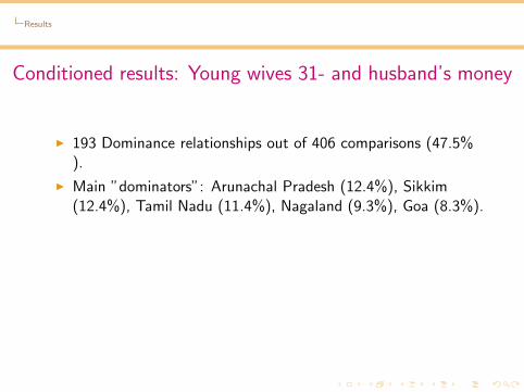
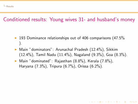
Conditioned results: Young wives 31- and husband’s money
I 193 Dominance relationships out of 406 comparisons (47.5%).
I Main ”dominators”: Arunachal Pradesh (12.4%), Sikkim(12.4%), Tamil Nadu (11.4%), Nagaland (9.3%), Goa (8.3%).
I Main ”dominated”: Rajasthan (8.8%), Kerala (7.8%),Haryana (7.3%), Tripura (6.7%), Orissa (6.2%).
I ”Top five” relationships: Nagaland>Tripura (0.2240),Sikkim>Tripura (0.2175), AruP>Tripura (0.2136),Nagaland>Rajasthan (0.2092), Manipur>Rajasthan (0.2037).
Results
Conditioned results: Young wives 31- and husband’s money
I 193 Dominance relationships out of 406 comparisons (47.5%).
I Main ”dominators”: Arunachal Pradesh (12.4%), Sikkim(12.4%), Tamil Nadu (11.4%), Nagaland (9.3%), Goa (8.3%).
I Main ”dominated”: Rajasthan (8.8%), Kerala (7.8%),Haryana (7.3%), Tripura (6.7%), Orissa (6.2%).
I ”Top five” relationships: Nagaland>Tripura (0.2240),Sikkim>Tripura (0.2175), AruP>Tripura (0.2136),Nagaland>Rajasthan (0.2092), Manipur>Rajasthan (0.2037).

Results
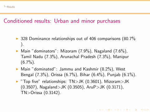
Conditioned results: Urban and minor purchases
I 328 Dominance relationships out of 406 comparisons (80.7%).
I Main ”dominators”: Mizoram (7.9%), Nagaland (7.6%),Tamil Nadu (7.3%), Arunachal Pradesh (7.3%), Manipur(6.7%).
I Main ”dominated”: Jammu and Kashmir (8.2%), WestBengal (7.3%), Orissa (6.7%), Bihar (6.4%), Punjab (6.1%).
I ”Top five” relationships: TN>JK (0.3601), Mizoram>JK(0.3507), Nagaland>JK (0.3505), AruP>JK (0.3171),TN>Orissa (0.3142).

Results
Conditioned results: Urban and minor purchases
I 328 Dominance relationships out of 406 comparisons (80.7%).
I Main ”dominators”: Mizoram (7.9%), Nagaland (7.6%),Tamil Nadu (7.3%), Arunachal Pradesh (7.3%), Manipur(6.7%).
I Main ”dominated”: Jammu and Kashmir (8.2%), WestBengal (7.3%), Orissa (6.7%), Bihar (6.4%), Punjab (6.1%).
I ”Top five” relationships: TN>JK (0.3601), Mizoram>JK(0.3507), Nagaland>JK (0.3505), AruP>JK (0.3171),TN>Orissa (0.3142).

Results
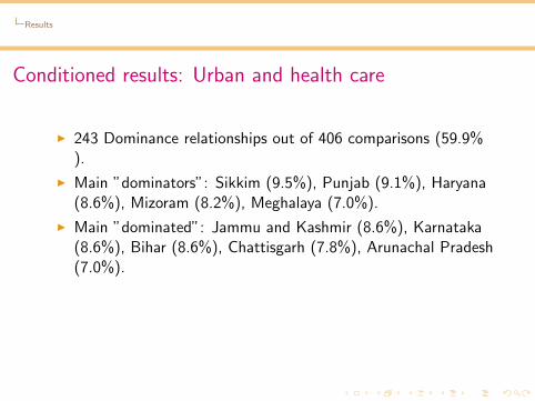
Conditioned results: Urban and health care
I 243 Dominance relationships out of 406 comparisons (59.9%).
I Main ”dominators”: Sikkim (9.5%), Punjab (9.1%), Haryana(8.6%), Mizoram (8.2%), Meghalaya (7.0%).
I Main ”dominated”: Jammu and Kashmir (8.6%), Karnataka(8.6%), Bihar (8.6%), Chattisgarh (7.8%), Arunachal Pradesh(7.0%).
I ”Top five” relationships: Sikkim> JK (0.2852), Sikkim>Bihar(0.2726), Punjab>JK (0.2570), Sikkim>Karnataka (0.2508),Mizoram>JK (0.2480).

Results
Conditioned results: Urban and health care
I 243 Dominance relationships out of 406 comparisons (59.9%).
I Main ”dominators”: Sikkim (9.5%), Punjab (9.1%), Haryana(8.6%), Mizoram (8.2%), Meghalaya (7.0%).
I Main ”dominated”: Jammu and Kashmir (8.6%), Karnataka(8.6%), Bihar (8.6%), Chattisgarh (7.8%), Arunachal Pradesh(7.0%).
I ”Top five” relationships: Sikkim> JK (0.2852), Sikkim>Bihar(0.2726), Punjab>JK (0.2570), Sikkim>Karnataka (0.2508),Mizoram>JK (0.2480).

Results
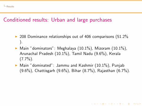
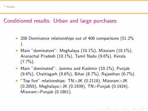
Conditioned results: Urban and large purchases
I 208 Dominance relationships out of 406 comparisons (51.2%).
I Main ”dominators”: Meghalaya (10.1%), Mizoram (10.1%),Arunachal Pradesh (10.1%), Tamil Nadu (9.6%), Kerala(7.7%).
I Main ”dominated”: Jammu and Kashmir (10.1%), Punjab(9.6%), Chattisgarh (9.6%), Bihar (8.7%), Rajasthan (6.7%).
I ”Top five” relationships: TN>JK (0.2118), Mizoram>JK(0.2055), Meghalaya>JK (0.1939), TN>Punjab (0.1924),Mizoram>Punjab (0.1861).

Results
Conditioned results: Urban and large purchases
I 208 Dominance relationships out of 406 comparisons (51.2%).
I Main ”dominators”: Meghalaya (10.1%), Mizoram (10.1%),Arunachal Pradesh (10.1%), Tamil Nadu (9.6%), Kerala(7.7%).
I Main ”dominated”: Jammu and Kashmir (10.1%), Punjab(9.6%), Chattisgarh (9.6%), Bihar (8.7%), Rajasthan (6.7%).
I ”Top five” relationships: TN>JK (0.2118), Mizoram>JK(0.2055), Meghalaya>JK (0.1939), TN>Punjab (0.1924),Mizoram>Punjab (0.1861).

Results
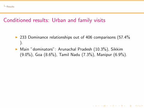
Conditioned results: Urban and family visits
I 233 Dominance relationships out of 406 comparisons (57.4%).
I Main ”dominators”: Arunachal Pradesh (10.3%), Sikkim(9.0%), Goa (8.6%), Tamil Nadu (7.3%), Manipur (6.9%).
I Main ”dominated”: Jammu and Kashmir (11.2%), Bihar(9.9%), Chattisgarh (8.2%), Jharkand (7.7%), MadhyaPradesh (7.7%).
I ”Top five” relationships: AruP>JK (0.3343), Sikkim>JK(0.2976), Goa>JK (0.2905), Mizoram>JK (0.2691),Nagaland>JK (0.2658).
Results
Conditioned results: Urban and family visits
I 233 Dominance relationships out of 406 comparisons (57.4%).
I Main ”dominators”: Arunachal Pradesh (10.3%), Sikkim(9.0%), Goa (8.6%), Tamil Nadu (7.3%), Manipur (6.9%).
I Main ”dominated”: Jammu and Kashmir (11.2%), Bihar(9.9%), Chattisgarh (8.2%), Jharkand (7.7%), MadhyaPradesh (7.7%).
I ”Top five” relationships: AruP>JK (0.3343), Sikkim>JK(0.2976), Goa>JK (0.2905), Mizoram>JK (0.2691),Nagaland>JK (0.2658).

Results
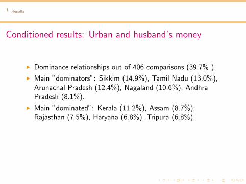
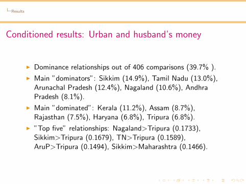
Conditioned results: Urban and husband’s money
I Dominance relationships out of 406 comparisons (39.7% ).
I Main ”dominators”: Sikkim (14.9%), Tamil Nadu (13.0%),Arunachal Pradesh (12.4%), Nagaland (10.6%), AndhraPradesh (8.1%).
I Main ”dominated”: Kerala (11.2%), Assam (8.7%),Rajasthan (7.5%), Haryana (6.8%), Tripura (6.8%).
I ”Top five” relationships: Nagaland>Tripura (0.1733),Sikkim>Tripura (0.1679), TN>Tripura (0.1589),AruP>Tripura (0.1494), Sikkim>Maharashtra (0.1466).

Results
Conditioned results: Urban and husband’s money
I Dominance relationships out of 406 comparisons (39.7% ).
I Main ”dominators”: Sikkim (14.9%), Tamil Nadu (13.0%),Arunachal Pradesh (12.4%), Nagaland (10.6%), AndhraPradesh (8.1%).
I Main ”dominated”: Kerala (11.2%), Assam (8.7%),Rajasthan (7.5%), Haryana (6.8%), Tripura (6.8%).
I ”Top five” relationships: Nagaland>Tripura (0.1733),Sikkim>Tripura (0.1679), TN>Tripura (0.1589),AruP>Tripura (0.1494), Sikkim>Maharashtra (0.1466).

Results
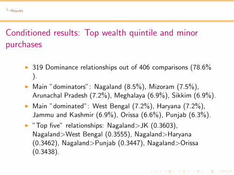
Conditioned results: Top wealth quintile and minorpurchases
I 319 Dominance relationships out of 406 comparisons (78.6%).
I Main ”dominators”: Nagaland (8.5%), Mizoram (7.5%),Arunachal Pradesh (7.2%), Meghalaya (6.9%), Sikkim (6.9%).
I Main ”dominated”: West Bengal (7.2%), Haryana (7.2%),Jammu and Kashmir (6.9%), Orissa (6.6%), Punjab (6.3%).
I ”Top five” relationships: Nagaland>JK (0.3603),Nagaland>West Bengal (0.3555), Nagaland>Haryana(0.3462), Nagaland>Punjab (0.3447), Nagaland>Orissa(0.3438).

Results
Conditioned results: Top wealth quintile and minorpurchases
I 319 Dominance relationships out of 406 comparisons (78.6%).
I Main ”dominators”: Nagaland (8.5%), Mizoram (7.5%),Arunachal Pradesh (7.2%), Meghalaya (6.9%), Sikkim (6.9%).
I Main ”dominated”: West Bengal (7.2%), Haryana (7.2%),Jammu and Kashmir (6.9%), Orissa (6.6%), Punjab (6.3%).
I ”Top five” relationships: Nagaland>JK (0.3603),Nagaland>West Bengal (0.3555), Nagaland>Haryana(0.3462), Nagaland>Punjab (0.3447), Nagaland>Orissa(0.3438).

Results
Conditioned results: Top wealth quintile and health care
I 256 Dominance relationships out of 406 comparisons (63.1%).
I Main ”dominators”: Mizoram (9.0%), Sikkim (9.0%), Punjab(8.6%), Haryana (8.2%), Meghalaya (7.4%).
I Main ”dominated”: Bihar (9.0%), Jharkand (8.2%),Karnataka (8.2%), Jammu and Kashmir (7.8%), ArunachalPradesh (7.0%).
I ”Top five” relationships: Sikkim>Bihar (0.2989), Sikkim>JK(0.2686), Mizoram>Bihar (0.2676), Sikkim>Jharkand(0.2607), Sikkim>Karnataka (0.2470).
Results
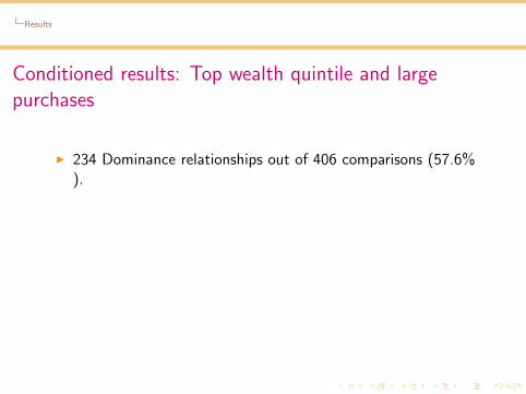
Conditioned results: Top wealth quintile and largepurchases
I 234 Dominance relationships out of 406 comparisons (57.6%).
I Main ”dominators”: Meghalaya (10.7%), Mizoram (10.3%),Nagaland (8.1%), Arunachal Pradesh (8.1%), Goa (7.7%).
I Main ”dominated”: Bihar (9.4%), Chattisgarh (7.3%), Punjab(7.3%), Haryana (6.8%), Jharkand (6.4%).
I ”Top five” relationships: Meghalaya>Punjab (0.1992),Meghalaya>JK (0.1937), Mizoram>Punjab (0.1936),Mizoram>JK (0.1881), Meghalaya>Bihar (0.1831).

Results
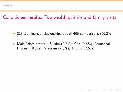
Conditioned results: Top wealth quintile and family visits
I 228 Dominance relationships out of 406 comparisons (56.2%).
I Main ”dominators”: Sikkim (9.6%), Goa (9.6%), ArunachalPradesh (8.8%), Mizoram (7.5%), Tripura (7.5%).
I Main ”dominated”: Bihar (9.6%), Chattisgarh (9.6%),Jammu and Kashmir (9.2%), Orissa (8.3%), Jharkand (7.5%).
I ”Top five” relationships: Goa>JK (0.2856), Sikkim>JK(0.2758), Tripura>JK (0.2610), AruP>JK (0.2390),Goa>Bihar (0.2318).
Results
Conditioned results: Top wealth quintile and family visits
I 228 Dominance relationships out of 406 comparisons (56.2%).
I Main ”dominators”: Sikkim (9.6%), Goa (9.6%), ArunachalPradesh (8.8%), Mizoram (7.5%), Tripura (7.5%).
I Main ”dominated”: Bihar (9.6%), Chattisgarh (9.6%),Jammu and Kashmir (9.2%), Orissa (8.3%), Jharkand (7.5%).
I ”Top five” relationships: Goa>JK (0.2856), Sikkim>JK(0.2758), Tripura>JK (0.2610), AruP>JK (0.2390),Goa>Bihar (0.2318).
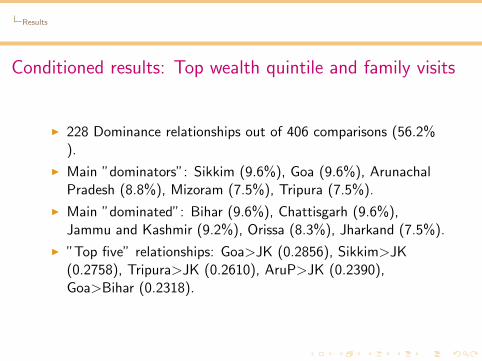
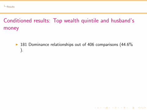
Results
Conditioned results: Top wealth quintile and husband’smoney
I 181 Dominance relationships out of 406 comparisons (44.6%).
I Main ”dominators”: Sikkim (13.3%), Arunachal Pradesh(12.2%), Nagaland (9.9%), Mizoram (8.3%), Goa (7.7%).
I Main ”dominated”: Kerala (11.6%), Orissa (10.5%), Haryana(8.8%), Karnataka (7.7%), Punjab (7.7%).
I ”Top five” relationships: Sikkim>Maharashtra (0.1604),AruP>Maharashtra (0.1423), Sikkim>Bihar (0.1301),Nagaland>Kerala (0.1262), Sikkim>Kerala (0.1248).
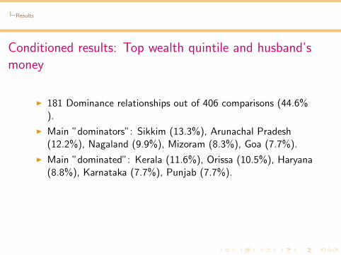
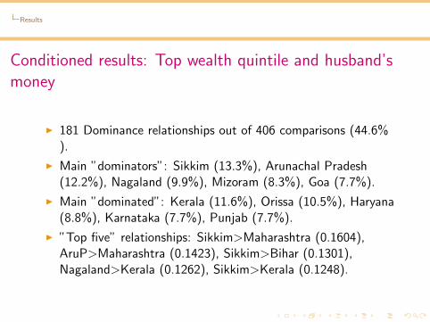

Concluding remarks
Concluding remarks
I Autonomy is a multifaceted phenomenon.
I The regional divides, and the pairwise state comparisons, reallydepend on the autonomy aspect/question.
I Most of the ”dominators” are from Northeaster India, most of thetime. But there are often important exceptions (e.g. Punjab is amain dominator on health autonomy).
I Most of the ”dominated” are from Northern India, most of thetime. But there are often important exceptions (e.g. Kerala is amain dominated state on husband’s money).
I Conditioning does not change the picture much (although we haveonly started exploring).

Concluding remarks
Concluding remarks
I Autonomy is a multifaceted phenomenon.
I The regional divides, and the pairwise state comparisons, reallydepend on the autonomy aspect/question.
I Most of the ”dominators” are from Northeaster India, most of thetime. But there are often important exceptions (e.g. Punjab is amain dominator on health autonomy).
I Most of the ”dominated” are from Northern India, most of thetime. But there are often important exceptions (e.g. Kerala is amain dominated state on husband’s money).
I Conditioning does not change the picture much (although we haveonly started exploring).
Concluding remarks
Concluding remarks
I Autonomy is a multifaceted phenomenon.
I The regional divides, and the pairwise state comparisons, reallydepend on the autonomy aspect/question.
I Most of the ”dominators” are from Northeaster India, most of thetime.
But there are often important exceptions (e.g. Punjab is amain dominator on health autonomy).
I Most of the ”dominated” are from Northern India, most of thetime. But there are often important exceptions (e.g. Kerala is amain dominated state on husband’s money).
I Conditioning does not change the picture much (although we haveonly started exploring).

Concluding remarks
Concluding remarks
I Autonomy is a multifaceted phenomenon.
I The regional divides, and the pairwise state comparisons, reallydepend on the autonomy aspect/question.
I Most of the ”dominators” are from Northeaster India, most of thetime. But there are often important exceptions (e.g. Punjab is amain dominator on health autonomy).
I Most of the ”dominated” are from Northern India, most of thetime. But there are often important exceptions (e.g. Kerala is amain dominated state on husband’s money).
I Conditioning does not change the picture much (although we haveonly started exploring).

Concluding remarks
Concluding remarks
I Autonomy is a multifaceted phenomenon.
I The regional divides, and the pairwise state comparisons, reallydepend on the autonomy aspect/question.
I Most of the ”dominators” are from Northeaster India, most of thetime. But there are often important exceptions (e.g. Punjab is amain dominator on health autonomy).
I Most of the ”dominated” are from Northern India, most of thetime.
But there are often important exceptions (e.g. Kerala is amain dominated state on husband’s money).
I Conditioning does not change the picture much (although we haveonly started exploring).

Concluding remarks
Concluding remarks
I Autonomy is a multifaceted phenomenon.
I The regional divides, and the pairwise state comparisons, reallydepend on the autonomy aspect/question.
I Most of the ”dominators” are from Northeaster India, most of thetime. But there are often important exceptions (e.g. Punjab is amain dominator on health autonomy).
I Most of the ”dominated” are from Northern India, most of thetime. But there are often important exceptions (e.g. Kerala is amain dominated state on husband’s money).
I Conditioning does not change the picture much (although we haveonly started exploring).

Concluding remarks
Concluding remarks
I Autonomy is a multifaceted phenomenon.
I The regional divides, and the pairwise state comparisons, reallydepend on the autonomy aspect/question.
I Most of the ”dominators” are from Northeaster India, most of thetime. But there are often important exceptions (e.g. Punjab is amain dominator on health autonomy).
I Most of the ”dominated” are from Northern India, most of thetime. But there are often important exceptions (e.g. Kerala is amain dominated state on husband’s money).
I Conditioning does not change the picture much (although we haveonly started exploring).

Concluding remarks
To do list
I Regional analysis North versus South, North-East versus each.
I Show results in maps?
I A dominance ”tree”.
I Look at joint ”autonomy deficiencies”: Through a latentvariable model (e.g. MIMIC, SEM)? Through a countingapproach? Other researchers have pursued, or are pursuing,similar paths.

Concluding remarks
To do list
I Regional analysis North versus South, North-East versus each.
I Show results in maps?
I A dominance ”tree”.
I Look at joint ”autonomy deficiencies”: Through a latentvariable model (e.g. MIMIC, SEM)? Through a countingapproach?
Other researchers have pursued, or are pursuing,similar paths.

Concluding remarks
To do list
I Regional analysis North versus South, North-East versus each.
I Show results in maps?
I A dominance ”tree”.
I Look at joint ”autonomy deficiencies”: Through a latentvariable model (e.g. MIMIC, SEM)? Through a countingapproach? Other researchers have pursued, or are pursuing,similar paths.