The Standard Model - Theoretisch-Physikalisches Institutaxm/sm2011.pdf · The current listing of our knowledge on the standard model of particle physics ... • Gauge theories in

The Standard Model

Lecture in SS 2011 at the FSU Jena

Axel Maas

2

Contents

1 Introduction 1

2 Basic phenomenology 3

2.1 Electromagnetic interactions . . . . . . . . . . . . . . . . . . . . . . . . . . 4

2.2 Strong interactions . . . . . . . . . . . . . . . . . . . . . . . . . . . . . . . 6

2.2.1 Gluons and color . . . . . . . . . . . . . . . . . . . . . . . . . . . . 6

2.2.2 Confinement, string breaking, and chiral symmetry breaking . . . . 7

2.2.3 Hadrons and glueballs . . . . . . . . . . . . . . . . . . . . . . . . . 8

2.2.3.1 Mesons . . . . . . . . . . . . . . . . . . . . . . . . . . . . 8

2.2.3.2 Baryons . . . . . . . . . . . . . . . . . . . . . . . . . . . . 10

2.2.3.3 Glueballs, hybrids, and the trouble with mixing . . . . . . 10

2.3 Conserved and almost conserved quantum numbers . . . . . . . . . . . . . 11

2.4 Weak interactions and parity violation . . . . . . . . . . . . . . . . . . . . 12

2.5 The Higgs effect . . . . . . . . . . . . . . . . . . . . . . . . . . . . . . . . . 14

2.5.1 The Higgs particle . . . . . . . . . . . . . . . . . . . . . . . . . . . 14

2.5.2 Classical breaking of the symmetry . . . . . . . . . . . . . . . . . . 15

2.5.3 Yukawa coupling . . . . . . . . . . . . . . . . . . . . . . . . . . . . 18

2.5.4 Weak gauge bosons . . . . . . . . . . . . . . . . . . . . . . . . . . . 19

2.6 Flavor physics, CP violations and the CKM matrix . . . . . . . . . . . . . 19

2.6.1 Generations . . . . . . . . . . . . . . . . . . . . . . . . . . . . . . . 19

2.6.2 Mixing and the CKM matrix . . . . . . . . . . . . . . . . . . . . . 20

2.6.3 CP violation . . . . . . . . . . . . . . . . . . . . . . . . . . . . . . . 22

2.6.4 Neutrino masses and neutrino oscillations . . . . . . . . . . . . . . . 22

3 Quantumelectrodynamics 25

3.1 Classical gauge theories . . . . . . . . . . . . . . . . . . . . . . . . . . . . . 26

3.2 The path integral . . . . . . . . . . . . . . . . . . . . . . . . . . . . . . . . 28

3.2.1 Heuristic introduction . . . . . . . . . . . . . . . . . . . . . . . . . 28

i

ii Contents

3.2.2 Functional analysis . . . . . . . . . . . . . . . . . . . . . . . . . . . 30

3.3 Matter fields . . . . . . . . . . . . . . . . . . . . . . . . . . . . . . . . . . . 32

3.3.1 Grassmann variables . . . . . . . . . . . . . . . . . . . . . . . . . . 33

3.3.2 Fermionic matter . . . . . . . . . . . . . . . . . . . . . . . . . . . . 36

3.4 Quantization of QED . . . . . . . . . . . . . . . . . . . . . . . . . . . . . . 36

4 QCD 41

4.1 Some algebra and group theory . . . . . . . . . . . . . . . . . . . . . . . . 41

4.2 Yang-Mills theory . . . . . . . . . . . . . . . . . . . . . . . . . . . . . . . . 45

4.3 QCD . . . . . . . . . . . . . . . . . . . . . . . . . . . . . . . . . . . . . . . 47

4.4 Quantization of Yang-Mills theories . . . . . . . . . . . . . . . . . . . . . . 48

4.5 BRST and asymptotic states . . . . . . . . . . . . . . . . . . . . . . . . . . 50

4.5.1 BRST symmetry . . . . . . . . . . . . . . . . . . . . . . . . . . . . 51

4.5.2 Constructing the physical state space . . . . . . . . . . . . . . . . . 53

5 Electroweak interactions and the Higgs 60

5.1 Assigning the quantum numbers . . . . . . . . . . . . . . . . . . . . . . . . 60

5.2 Hiding local symmetries . . . . . . . . . . . . . . . . . . . . . . . . . . . . 63

5.3 Quantizing the Abelian-Higgs model . . . . . . . . . . . . . . . . . . . . . 66

5.4 Hiding the electroweak symmetry . . . . . . . . . . . . . . . . . . . . . . . 68

5.5 Fermion masses . . . . . . . . . . . . . . . . . . . . . . . . . . . . . . . . . 71

5.6 The Glashow-Salam-Weinberg theory in general . . . . . . . . . . . . . . . 72

5.7 The electroweak sector of the standard model . . . . . . . . . . . . . . . . 74

5.8 Quantizing the electroweak theory . . . . . . . . . . . . . . . . . . . . . . . 78

5.8.1 Non-Abelian case with hidden symmetry . . . . . . . . . . . . . . . 78

5.8.2 Gauge-fixing the electroweak standard model . . . . . . . . . . . . . 79

5.8.3 The physical spectrum with hidden symmetry . . . . . . . . . . . . 80

6 Examples in perturbation theory 83

6.1 Cross-sections and decays . . . . . . . . . . . . . . . . . . . . . . . . . . . 83

6.2 Perturbative description of processes . . . . . . . . . . . . . . . . . . . . . 85

6.2.1 General construction . . . . . . . . . . . . . . . . . . . . . . . . . . 85

6.2.2 Example at tree-level . . . . . . . . . . . . . . . . . . . . . . . . . . 94

6.3 Ward-Takahashi and Slavnov-Taylor identities . . . . . . . . . . . . . . . . 95

6.3.1 Ward-Takahashi identities . . . . . . . . . . . . . . . . . . . . . . . 95

6.3.2 Slavnov-Taylor identities . . . . . . . . . . . . . . . . . . . . . . . . 97

6.4 Radiative corrections . . . . . . . . . . . . . . . . . . . . . . . . . . . . . . 99

Contents iii

6.4.1 Cutoff regularization . . . . . . . . . . . . . . . . . . . . . . . . . . 100

6.4.2 Renormalization . . . . . . . . . . . . . . . . . . . . . . . . . . . . . 101

6.4.3 Counter-term structure . . . . . . . . . . . . . . . . . . . . . . . . . 103

6.4.4 Renormalization schemes and dimensional transmutation . . . . . . 105

6.4.5 Dimensional regularization . . . . . . . . . . . . . . . . . . . . . . . 107

6.4.6 Running couplings, Landau poles, and asymptotic freedom . . . . . 110

Chapter 1

Introduction

The standard model of particle physics is the to-date most successful theory of particles and

interactions. It describes accurately the dynamics of particles from scales of the order of

meters down to about 10−23 m, the smallest length scale yet probed. Part of its predictions

have been tested to a numerical precision of about 10−10 successfully, and some general

consequences even up to 10−40. The current listing of our knowledge on the standard

model of particle physics is available by the particle data group at http://pdg.lbl.gov/,

the authoritative summary of current knowledge.

However, there are quite a number of reasons to believe that the standard model is

only a low-energy effective theory, where low could be as small as a couple of hundred

GeV up to 1019 GeV. Its internal consistency and astrophysical observations suggest that

its range of validity may end rather earlier than latter, but this is an ongoing experimental

and theoretical endeavor to find the limits of this model, without proven success so far.

To understand the questions posed by the current form of the standard model, and what

could replace it requires first an understanding of how it works, and why it is so successful.

This is the aim of the present lecture. An introduction to beyond-the-standard-model can

be found, e. g., in my lecture on beyond-the-standard-model physics.

This introduction aims primarily on giving an overview of the phenomenology and the

theoretical structures of the standard model. In the first part the basic phenomenology

will be introduced. It will exhibit the four central sectors of the model, electromagnetism,

weak interactions, strong interactions, and the Higgs sector. These affect the matter inside

the standard model, the quarks and leptons, which will be introduced. These have very

particular connections to these forces, which will be elucidated in detail. This combination

shows very interesting features and phenomena, which will be shortly introduced.

After this more phenomenological overview, the second part of this lecture will give an

introduction to the quantization of the standard model, given that even quantum effects

1

2

have been observed with very high precision. The basic ingredient is the generalization of

Maxwell’s theory, so-called gauge theories of Yang-Mills type. Their quantization with and

without matter fields will require the most formal developments in this lecture. Technically,

it is most convenient to use for this the path integral formalism, which will be developed

to the extent necessary. In addition, some more formal aspects of such theories, like the

asymptotic state space, will be introduced to make clear the distinction between auxiliary

fields and quasi-physical observables. Finally, to catch up with current developments, some

basic notions on the perturbative determination of observables and cross sections will be

presented, alongside with some more concepts of central importance in performing explicit

calculations.

There is a vast literature on the standard model and its theoretical basis, quantum

(gauge) field theories. Here, only the books will be listed which have been used during the

preparation of this course, but there is a wealth of further very good textbooks available,

which should offer for everyone a suitable presentation of the subject. The books used

here were (in order of increasing complexity)

• High-energy physics by D. Perkins (Addison-Wesley)

• Gauge theories in particle physics by I. Aitchison and A. Hey (IOP publishing)

• An introduction to quantum field theory by M. Peskin & D. Schroeder (Perseus)

• Gauge theories of the strong and electroweak interactions by Bohm et al., (Teubner)

• Path integral methods in quantum field theory by J. Rivers (Cambridge)

• Group structure of gauge theories by L. O’Raifeartaigh (Cambridge)

• The quantum theory of fields I & II by S. Weinberg (Cambridge)

This script cannot replace any of these books, and should merely be regarded as a guide

to the literature, and a list of relevant topics.

Chapter 2

Basic phenomenology

Before delving too deep into the technical details of the standard model, it is useful to first

get an overview of the major different phenomena which are described by the standard

model, without getting into technical details. Otherwise, it is rather simple to get lost

in the details without getting the big picture. Therefore, the different sectors, forces,

particles, and phenomena of the standard model will be introduce in the following in a

more heuristic way, before attempting to describe them in more precise mathematical

language.

It should be noted that it was a rather long journey, taking about 40 years, for the

construction of the standard model. In this time, hundreds of different models of particle

interactions have been considered and then dropped because they were inconsistent with

the experimental observations. The standard model is the simplest remaining theory which

is able to describe all observations made so far. However, it has still predictions, and even

a particle, the Higgs, which have not been observed yet, so it can still be falsified, or at

least shown to be incomplete. Nonetheless, the number of phenomena described is vast,

and even the list to be shown here is by far not exhaustive, but can only give a brief

glimpse of the more prominent phenomena.

The approach followed here is rather top-down, i. e. with hindsight, rather than to

trace out the complicated story of the discovery of the standard model. To learn about

the involved history and the reasoning for the construction of the standard model, the

corresponding literature on science history should be consulted. In particular, it is worth-

while to learn how to make mistakes and learn from them, which can be an invaluable

asset for ones own research.

A last remark is that despite the fact that we are able to write down the standard model

in closed form, we are far away from the point were we would be able to calculate any

given quantity with a given precision in the standard model. Many questions we can yet

3

4 2.1. Electromagnetic interactions

answer at best qualitative rather than quantitative. Only in rather special circumstances

we are able to make precise statements, which are on equal footing with the precision of

experiments. These are usual cases which have a very clean, very special environment,

where only a small part of the standard model contributes appreciably.

2.1 Electromagnetic interactions

The most well known interaction, aside from gravity which is not part of the standard

model, is electromagnetism. All of chemistry and even the fact that one can write on a

blackboard is an electromagnetic effect. Its covariant description is performed using the

field-strength tensor Fµν , given as

Fµν = ∂µAν − ∂νAµ,

with the vector potential Aµ. The conventional field strength of the electric and magnetic

fields are given by

~Ei = − ∂

∂tAi − ∂iA0

~Bi = (~∇× ~A)i.

When using an action principle, the action S is then given by

S =

∫

d4xL,

with the Lagrangian density

L = −1

4FµνF

µν .

The usual Euler-Lagrange equations of motion

∂µδL

δ∂νAν− δLδAµ

= 0

of this system are then the Maxwell equations.

After quantization, the quanta of this theory, which will be the quanta of the then so-

called gauge field Aµ, are the photons. These will turn out to be massless bosons, which

have spin 1. Since they are massless, they have actually only two possible polarizations

for their z component, +1 and -1, and 0 is not possible. The reason for this can be seen

rather directly to be a consequence of each other.

In classical physics, an electromagnetic current jµ can be coupled to the electromagnetic

field by the (minimal) interaction Lagrangian

L = −ejµAµ, (2.1)

Chapter 2. Basic phenomenology 5

where the current carries electric charge e. As in quantum mechanics, this current can be

written in the form

jµ = ψγµψ,

where ψ denotes the matter fields, which is charged. Most of the electromagnetically

charged particles in the standard model are fermions with spin 1/2, and thus for everyone

exists a corresponding anti-particle. Then, the ψ are spinors, and the γµ are thus the

Dirac matrices. However, there are also electrically charged bosons of spin 0 and 1 in the

standard model, to be introduced later.

In the standard model of particle physics, there are nine fermionic matter fields which

are charged, which split into two sets. The one set are six quarks, or six quark flavors.

These are called up (with a mass of 2-3 MeV), down (4-6 MeV), strange (80-130 MeV),

charm (1270(10) MeV), bottom (4190(200) MeV), and top (172000(1500) MeV). The sec-

ond set is denoted leptons, the lepton flavors being the well-known electron (0.5 MeV),

muon (106 MeV), and tauon (1777 MeV). These nine particles behave the same with re-

spect to electromagnetism, and the splitting comes from the fact that they will behave

differently under the remaining interactions.

One of the remarkable facts of the standard model is that the electric charge may be

different for all of these particles, i. e. eu must not be the same as ee, and this is accom-

modated by writing Qie, where Qi is the charge of the particle i in units of the electron’s

charge e. When measured, it turns out that the charges Qi are actually not arbitrary, but

take ratios of small integer numbers. In particular, Qi is 1 for all leptons, while it is 2/3

for the up quark, the charm quark, and the top quark, and it is -1/3 for the down quark,

for the strange quark, and for the bottom quark. The corresponding anti-particles have

the negative of these charges. There is no explanation for this fact in the standard model.

However, it turns out that the standard model can only be mathematically consistent if

and only if the particles have precisely these relative sizes, and that there is always a

triple of particles with charges 1, 2/3 and -1/3. This is the so-called anomaly cancellation

condition, which will only be discussed at the very end of this lecture.

A second important property of the electromagnetic interactions is the presence of γµ

in the expression (2.1). Such a coupling is called vectorial. It is not the only possibility,

and others will appear in other sectors of the standard model. The important point is that

such a coupling is parity conserving, since (2.1) is. This follows from the fact that jµ is

behaving like a vector under parity transformations, as is known from the properties of the

Dirac equation and the Dirac matrices. Since also the vector potential behaves as a vector

under parity transformation, the total expression is invariant under parity transformation.

If instead the coupling would be, e. g., to the magnetic field, which is a pseudo-vector, the

6 2.2. Strong interactions

coupling would have changed sign under a parity transformation, and thus would violate

parity.

2.2 Strong interactions

The second interaction of the standard model is the so-called strong force or nuclear

force, with its quantized theory called quantumchromodynamics (QCD). This force is

what compensates the electromagnetic force in nuclei such that the positively charged

protons can be bound together to form nuclei.

2.2.1 Gluons and color

Similarly to the electromagnetic interactions, the strong interactions are mediated by

massless particles and via a vectorial coupling. Only the quarks, thus distinguishing them

from the leptons, are charged under this new force, and thus react directly to it. However,

in contrast to electromagnetism, there is not only one charge and anti-charge, but there

are three. These are called, for historical reasons, red, blue, and green (or sometimes

also yellow). There are correspondingly three anti-charges, called anti-red, anti-blue, and

anti-green. Thus, each quark exists in three sub-species, one for each color. There are two

more features which make quark charges different from electromagnetic charges. One is

that not only a charge and an anti-charge yield a neutral object, but also three different

charges or three different anti-charges combine to a neutral object. Thus, the combination

of a red quark, a green quark, and a blue quark is neutral with respect to the strong

interactions. The second difference is that color charge is not an observable, in contrast to

electric charge. While electric charge is classically invariant under a gauge transformation,

this is not the case for a color charge. This has rather profound consequences, which will

be experienced when quantizing the theory.

The interactions between color charges is mediated by massless vector, i. e. spin one,

particles, so-called gluons. In contrast to photons, the gluons also carry charges of the

forces which they mediate. There are eight different gluon charges, but no anti-charges.

These eight gluon color charges are all different from the three quark charges or quark anti-

charges. It is thus not possible to combine quark color charges and gluon color charges

to obtain a neutral object. It is, however, possible to combine two gluon color charges to

obtain a neutral object. A second consequence is that gluons can interact with themselves,

even if no matter particles are present. Thus, a theory of only gluons is non-trivial in itself,

and is called Yang-Mills theory. This theory will play a central role in the quantization of

the standard model of particle physics.


2.2.2 Confinement, string breaking, and chiral symmetry break-

ing

The strong force is actually much stronger than the electromagnetic force. It is thus

surprising that it not dominates our experience of the world, and is indeed only visible

when investigating nuclear and subnuclear effects. The reason is the so-called confinement

phenomena. This theoretical concept was constructed to explain the experimental fact that

no experiment has ever detected a free quark or a free gluon, actually up to a precision

of about 10−40 and 10−20, respectively. Confinement denotes just this observation: There

are no free quarks or gluons. The theoretical understanding from first principles of this

observation is a very complicated and challenging task, and not yet completed.

The simplest idea of why confinement occurs is rooted in the following observation: The

strong interactions become actually stronger with increasing distance. This is completely

different to electromagnetism, which gets weaker with distance. On the other hand, at

very high energies, and thus subnuclear scales, the strong interaction almost ceases. This

property of the strong interactions is called asymptotic freedom. It is thus imagined that

the force becomes at scales of about the size of a small nuclei, like the hydrogen, so strong

that it is not possible to escape anymore from a neutral object. Of course, this is a

heuristically and rather classically view, but should mediate the central idea.

Thus, as a consequence of confinement, quarks and gluons only appear in color-neutral

bound states in nature, so-called hadrons and glueballs. When trying to pull the con-

stituents of such a bound state apart by investing enough energy, such bound states react

by breaking into further bound states, instead of breaking apart. Thus, confinement pre-

vents the escape of a colored object perfectly. The phenomena of this particle production

is called string breaking. This name originates from the picture that when trying to break

a bound state apart, the force between the colored constituents is collimated into a flux

tube, which decays into new bound states once enough energy is invested into these flux

tubes. Again, this is only a heuristic view of a more complicated dynamical process.

This enormous strength of the strong interactions has another consequence. Return to

the simplest Lagrangian for a free fermion, which is given by

L = iψγµ∂µψ.

The equation of motion of this Lagrangian is the Dirac equation. Using γ5 = iγ0γ1γ2γ3,

this Lagrangian is invariant under the transformation exp(iγ5α) with α an arbitrary pa-

rameter. This symmetry is called a chiral symmetry. A mass term breaks this symmetry

explicitly, but the masses of the light quarks, up and down, are so small that this break-

ing can be almost neglected. However, the strong interactions break this symmetry also


spontaneously, similarly to the magnetization of a magnet. As a consequence, it is found

that the effective mass of the quarks is increased by about 300 MeV. Thus, for all practical

purposes the up and down quarks have a mass of about 300 MeV, and the strange quark

of about 400 MeV. This will have quite an impact on the masses of bound states. Again,

this effect is not yet fully understood, as the strength of the interactions and the presence

of confinement, which is often conjectured to be in close connection to chiral symmetry

breaking, make an explicit calculation of these phenomena complicated.

2.2.3 Hadrons and glueballs

As described previously, quarks and gluons can only appear in neutral, i. e. colorless,

bound states. For quarks, there are two obvious combinations, which are color-neutral.

These are the combination of a quark and an anti-quark, which form a so-called meson.

The combination of three quarks forms a baryon, and of three anti-quarks an anti-baryon.

Of course, a combination of two quarks and two anti-quarks would also be color-neutral

as would be a suitably chosen combination of four quarks and one anti-quark, or even

more quarks and anti-quarks. These so-called tetraquarks and pentaquarks have not been

observed with certainty to date. It is thus unclear, whether such combinations would be

sufficiently stable to be observable at all. For sure, these states would not be stable, but

the question remains whether they would live long enough to be called a bound state.

These multi-quark states are also affected by the problem of mixing, discussed below.

2.2.3.1 Mesons

This leaves the mesons and baryons to ponder. The mesons are bosons as a bound state

of two fermions. The two constituents of the meson can be either of the six quark flavors,

where a combination of two bottom quarks or two charm quarks are often called quarkonia.

If a meson is combined from twice the same quark it is also electrically charge neutral. If it

is combined from two different flavors, it can be either charge neutral, if both particles have

the same absolute value of the electric charge (e. g. a up and an anti-charm), positively

charged (e. g. a up and an anti-down) or negatively charged (e. g. a down and an anti-

up) with, within experimental uncertainties, precisely one unit of the electron charge.

Furthermore, if a meson consists of a quark and an anti-quark of the same flavor, it is

often said to have a hidden flavor, e. g., hidden charm. If this is not the case, in particular

if one of the flavors is much heavier than the other, it is said to have an open flavor, e. g.,

open charm.

The simple estimate for a bound state mass would be simply twice the constituent


mass. For mesons made from heavy quarks this turns out to be approximately correct.

For the lightest mesons, this is not the case. The reason is that these mesons act as so-

called Goldstone bosons for the broken chiral symmetry. This concept will be discussed

in much more detail when coming to the Higgs effect, where it is possible to illuminate

the concept with much simpler technical details. For now, it suffices to say that for every

spontaneously broken global symmetry, here the chiral symmetry, there must be a certain

number of massless particles. If all quarks would be massless, this number would be 35.

However, the explicit breaking due to the quark masses increases the mass significantly

for most of these Goldstone bosons, making them almost indistinguishable from ordinary

bound states. Only the nine lightest mesons have an anomalously small mass due to this

Goldstone effect.

The lightest of these are the pions, which have about 140 MeV of mass. There are

three, made of the quarks ud, du and a third, neutral one. This last one is useful to

elucidate the concept of mixing.

Take an arbitrary quantum system. If two states, say |1 > and |2 >, have the same

conserved quantum numbers, both can mix, i. e., it is possible for a state |a > with the

same quantum numbers to be a linear combination of both states,

|a >= α|1 > +β|2 >,

such that |α|2 + |β|2 = 1. The third pion is precisely such a mixing from the two combi-

nations uu and dd. Similarly, all other neutral mesons can mix. In principle, also ss or cc

etc. can mix with the neutral pion. However, their contributions, i. e. pre-factors like α

and β, are found to be negligibly small.

Returning to the original subject, there are six further such pseudo-Goldstone bosons,

which are surprisingly light. These are two charged kaons with mass of about 500 MeV,

and two neutral kaons with about the same mass. These are the combinations us, su for

the charged ones and ds and sd for the neutral ones. Then there is the η meson, which

mixes besides uu, dd also ss. Its mass is about 550 MeV. The last one is also such a

mixture, but with a different composition (a different value of α, β,...). However, this η′

turns out to be unexpectedly heavy, about 960 MeV. The reason for this is a quantum

anomaly, which will be discussed much later.

Besides these ground states there are also excited states, similarly to the excited states

of the hydrogen atom. In this case the quarks have additional relative orbital angular

momentum. The most prominent example is arguably the ρ meson, which is a combination

of up and down quarks with total spin one instead of zero, and a mass of about 770

MeV. It decays quickly into the lighter ground state mesons, but other excitations can be

essentially meta-stable on the time-scale of elementary particles. Indeed, similar to atoms


(or molecules), a complete spectroscopy of meson states (and also baryon states) can be

obtained, though being much more complicated in detail. The cleanest spectroscopy of

such systems has so far been possible for the quarkonias of charm and bottom mesons,

for which several excited states with different radial and angular quantum numbers are

known.

2.2.3.2 Baryons

The next type of bound states are baryons, which are made up of three quarks. To be color-

neutral, these three quarks have to have all different colors. As a consequence, using an

anti-symmetric wave function in color space, the Pauli principle is fulfilled, and otherwise

any combination of three quarks (or three antiquarks for an antibaryon) are permitted.

Incidentally, this was also one of the first indirect evidences for the existence of color.

Thus, the electric charge of a baryon can be -1, 0, 1, and 2. The spins can be aligned or

not, giving ground states with spins between -3/2 and 3/2, and thus baryons, in contrast to

mesons, are fermions. Note that the baryons with spin ±3/2 are generically heavier than

those with spin ±1/2. The most prominent baryons are the proton, the hydrogen nucleus,

and the neutron. These are made up of the combinations uud and udd, respectively,

leading to their electric charges of zero and one, respectively.

The masses of the ground-state baryons are roughly given by the masses of the quarks

including the effect of chiral symmetry breaking. Thus the mass of the proton is about

3 + (300 + 3)× 3, which is 915, just slightly lower than the actual value of 938 MeV, and

the neutron ends up at 918 MeV compared with 939.5. There are also excited states of

baryons, with mass differences usually some tens of MeV compared to lower states. As

with mesons, excited baryons usually decay quickly, but in exceptional circumstances they

may be stable over long times for kinematic and other reasons.

2.2.3.3 Glueballs, hybrids, and the trouble with mixing

As noted, since gluons interact with themselves, they can even bind together to a third

type of bound state, the so-called glueballs. These consists of two gluons of appropriately

selected colors. However, in contrast to both baryons and mesons, such glueballs would

again be bosons, as they consist of two bosons. As with baryons and mesons, it is possible

to obtain also excited states. Calculations indicate that such glueballs would be quite

heavy, about 1.5 GeV for the lightest ones. In contrast to both mesons and baryons,

however, glueballs have not been observed.

The are two reason for this. One is that such heavy glueballs could easily decay into

two mesons. The second is mixing. Since most glueballs have the same quantum numbers


as mesons, such states are mixtures

|mix >= α|meson > +β|glueball > .

To the best of our knowledge all such states are more or less dominated by the mesonic

part, and only few states have yet been observed with properties which suggest that their

glueball content would be rather large. These are so-called f mesons, which also have

masses around 1.5 GeV. Unfortunately, such heavy particles decay quickly into lighter

mesons, making a precise experimental analysis complicated and constitute a remaining

challenge.

There are further states, which could mix in, in particular states which consist of two

quarks and one or more gluons, qqg, so-called hybrids. Such object can be color-neutral,

and so the full mixing for the appropriate choice of quantum numbers is then

|mix >= α|meson > +β|glueball > +γ|hybrid >,

complicating things further.

The same problem is also occurring when investigating tetraquarks and pentaquarks.

Usually, these configurations can also mix with mesons or baryons, and thus it is very

hard to determine the existence of such states. In all cases discussed so far, however, there

exist some rare configurations of quantum numbers which can only manifest themselves

in glueballs, hybrids, tetraquarks or pentaquarks. unfortunately, such particular combina-

tions are often very heavy, and thus both their production is very complicated and they

tend to decay quickly. Thus, there is no commonly accepted observation of any of such

more complicated states. A further problem is that such states, though not mixing with

ordinary mesons and baryons, can mix with so-called molecular states, i. e., states which

consist of two orbiting mesons or a meson and a baryon, similar to simple atoms. It is very

hard to distinguish these concepts cleanly, both experimentally and theoretically, leaving

a wide field open for the future.

2.3 Conserved and almost conserved quantum num-

bers

At this point it is useful to collect the quantum numbers actually present in the theory

so far, as in the following the violation of quantum numbers will become important. It

should be started with those quantum numbers which are absolutely conserved in the

standard model, i. e., no process is yet known which does not conserve them. These are

12 2.4. Weak interactions and parity violation

the spin of particles, the electric charge, and the color charge. There is also the so-called

CPT symmetry, which consist of a parity transformation, an exchange of particle and

anti-particles, and an inversion of, more or less, momenta, which is exactly conserved.

Then there are a number of quantum numbers which are conserved up to now, but will

no longer be conserved in the full standard model. Their conservation is partly only very

mildly violated, such that essentially no process has been observed yet that is violating it.

To this type of processes belong the number of leptons and the number of quarks,

which are associated with the lepton number L (each lepton carries a lepton number of

one, each antilepton carries a lepton number of minus one), and the baryon number B

carried by quarks (1/3 for each quark and -1/3 for each antiquark). Thus mesons and

glueballs have baryon number zero, and baryons ±1, hence the name. These quantum

numbers are individually not conserved in the standard model, but the violation is so

weak that for all practical purposes (and in all direct experimental observations so far)

their violation can be ignored. The combined number L+B is absolutely conserved.

There are then a number of quantum numbers, which will be violated in the following.

The first quantum number is flavor, i. e., the number of particles of any lepton or quark

flavor. Both electromagnetic and strong interactions conserve flavor, and thus the number

of, e. g., charm quarks will not change in electromagnetic or strong processes, though

they could kinematically decay in three up quarks. The next quantum numbers are par-

ity, charge parity, and time reversal parity. I. e., whether processes are unchanged under

a parity transformation, an exchange of particles and antiparticles, and the inversion of

momenta, respectively. All these symmetries are respected by both strong and electro-

magnetic interactions, but are violated in the standard model by further interactions.

Of course, the one symmetry violated already by the strong interactions is the chiral

symmetry, but this is also broken explicitly. However,this explicit breaking is actually also

a dynamical breaking after including the Higgs below.

2.4 Weak interactions and parity violation

The third force in the standard model is the weak force, which is, e. g., responsible for

nuclear β decays. This interaction is mediated by three vector bosons, the electrically

neutral Z boson and the electrically charged W+ and W− bosons. In contrast to the

photons and the gluons, these are not massless, but very massive, having masses of size 91

GeV and 80 GeV, respectively. Under the weak force all quarks and leptons are charged.

In addition, there are three more matter particles, which are also charged under this

interactions, commonly denoted as neutrinos. There are three types of them, the electron


neutrino, the muon neutrino, and the tauon neutrino, and the corresponding antiparticles.

As the names of these fermions suggest, these particles carry a positive lepton number,

and are associated to the electron, the muon and the tauon, as will be discussed in more

detail later. Also discussed later will be the masses of these particles, for which is only

known than it is less than 0.3 eV, but at least two of them have a non-zero mass, and all

three have different masses.

Similarly as for the strong interactions, there are two different weak charges and cor-

responding anticharges for the weak interactions, while the gauge bosons carry each a

distinct weak charge different from the charges of the matter particles. However, here the

similarity ends. The main reason is that the weak interactions are parity violating: In

contrast to the strong and electromagnetic vectorial theories the weak interaction makes

a difference between left and right, and is therefore called a chiral theory.

This manifests itself in a different coupling structure than in those cases, which take

the form (2.1). In contrast, here the the coupling is

Bµψγµ1− γ5

2ψ, (2.2)

where Bµ is any of the weak bosons. It is always possible to write a spinor in terms of a

left-handed and a right-handed component

ψL =1− γ5

2ψ

ψR =1 + γ5

2ψ,

where handedness is with respect to the helicity of the particle, i. e., the projection of the

spin of a particle unto its momentum - the would-be angular momentum of the spin makes

a left-handed or a right-handed screw with respect to the momentum in the corresponding

cases.

From this follows that the coupling (2.2) only connects left-handed fermions with the

weak interactions, and right-handed fermions are uncharged. Thus, there is a difference

between different directions, and thus parity is not conserved in the weak interactions:

Nature makes a difference between left and right. As a consequence, only left-handed

fermions carry the two different weak charges, and it is said they form a doublet under

the weak interactions. At the same time, the right-handed fermions do not carry a weak

charge, they form a singlet. For that reason, right-handed neutrinos do not interact with

any of the forces in the standard model introduced so far.

This parity violation has also a further consequence: It is not possible to give fermions

a mass. This can be seen as follows. The Dirac equation for fermions, like leptons and

14 2.5. The Higgs effect

quarks, has the form

0 = (iγµDµ −m)ψ =

(

iγµDµ +1− γ5

2m+

1 + γ52

m

)

ψ.

The problem comes now from the fact that the weak interactions are a gauge interaction,

and it is possible to change the gauge fields without changing the physics. The covariant

derivative Dµ, which includes the coupling (2.2), respects this symmetry, and so does the

spinor (1−γ5)/2ψ. However, the spinor (1+γ5)/2ψ is a singlet under such a transformation.

Hence, not all terms in the Dirac equation transform correctly. As will be discussed below,

such a symmetry is essential for describing the weak force consistently. Hence, such a mass

term is incompatible with this description of the weak force. Another way of observing

this is that the mass term for fermions in Lagrangian can be written as

Lmψ = m(ψLψR − ψRψL),

and therefore cannot be invariant, if only left-handed fermions change.

This obstacle was the reason to introduce the Higgs particle, which solves this problem

dynamically.

2.5 The Higgs effect

2.5.1 The Higgs particle

The Higgs particle φ is the only not yet observed particle in the standard model. The only

thing sure is that its mass is larger than 115 GeV, and it is likely not between 158 and

173 GeV. It is a scalar particle, which has a zero electric charge, but is interacting with

the weak bosons. Thus, it has a weak charge. It furthermore interacts with fermions of

flavor f with a coupling which is of the form

gfφψfψf , (2.3)

a so-called Yukawa coupling. In the standard model, it turns out that the coupling gf

is indeed specific for each flavor, i. e., each flavor of quarks and leptons couples with a

different strength to the Higgs, though the numeric values of some of the couplings to

neutrinos are not yet known, and only upper limits can be given. Finally, this coupling

is left-right symmetric, i. e., it has the same strength for left-handed and right-handed

quarks, and is thus not parity violating.

This Higgs particle can now be used to provide the mass to all the fermions, despite

the limitation of the weak interactions. The basic mechanism is the so-called Higgs effect.


It is essentially based on the idea that the Higgs forms a condensate, and thus the Higgs

field has a non-zero expectation value < φ > 6= 0, and the interaction with this condensate

provides an apparent mass to the particles, though not a real one.

To understand this, it is useful to investigate first a simple example, before discussing

the full standard model case.

2.5.2 Classical breaking of the symmetry

Take a single scalar field φ. The requirement that the expectation value of a field should

be non-vanishing in the vacuum translates into the requirement that the corresponding

energy of such a state must be lower than for a vanishing field. The only consistent

potential which enforces, at least at tree-level, this behavior is

V (φ) = −1

2µ2φ2 + ωφ3 +

1

2

µ2

f 2φ4. (2.4)

The φ3 is found to be in contradiction to experiment for the standard model, and will

therefore also here no longer be considered, and thus ω is set to zero.

This potential has a minimum at φ = ±f/√2, V (±f/

√2) = −f 2µ2/8. On the other

hand, it has a maximum at φ = 0. Therefore, (weak) quantum fluctuations will always

drive the system away from φ = 0 and into the minimum. Of course, quantum effects will

also shift the minimum away from f , and it cannot be excluded a-priori that these could

not distort the maximum sufficiently such that φ = 0 would again be a minimum. In fact,

examples are known where this is the case. However, experimental tests seem to indicate

that this is not the case for the generalization to the standard model. Hence, it will be

assumed henceforth that this is not happening.

The potential (2.4) has actually two equivalent minima, at ±f/√2, if ω = 0. The

potential is Z2 symmetric. Nonetheless, the groundstate has to have a unique value for

the field. Therefore, the ground-state will be either of both minima. By this, the symmetry

of the system seems to be broken. However, this is not the case: It is just not apparent

anymore, it is hidden. Nonetheless, the situation is often denoted (in an abuse of language)

as a spontaneous breakdown of the symmetry. This is similar to an ordinary ferromagnet:

There, rotational invariance seems to be broken by the magnetization. However, the

direction of the magnetization is chosen randomly, and an averaging over many magnets

would restore the symmetry again. In principle, it would be possible to think about mixing

both vacuum states in one way or the other. This would make the symmetry more explicit,

but there is no need to. It is a freedom to select either of the minima as a starting point,

since they are equivalent.


For the standard model, this turns out to be too simplistic, since the Higgs interacts

with the weak gauge bosons. Therefore, at the very least a scalar charged under the weak

interactions will be necessary. Actually, it will be necessary to upgrade it at least to a

doublet later on. The potential for such a charged scalar field is similarly given by

V (φ, φ+) = −1

2µ2φ+φ+

1

2

µ2

f 2(φ+φ)2. (2.5)

A cubic term φ2φ+ + φ+2φ has been omitted directly. In this case, a phase symmetry is

present, i. e., the theory is invariant under the replacement

φ → e−iθφθ small= φ− iθφ+O(θ2)

φ+ → eiθφ+ θ small= φ+ + iθφ+ +O(θ2).

To analyze the situation further, it is useful to rewrite the complex field in terms of its

real and imaginary part

φ = σ + iχ,

and correspondingly for its hermitiean conjugate. The Lagrangian then takes the form

L =1

2(∂µσ∂

µσ + ∂µχ∂µχ) +

µ2

2(σ2 + χ2)− 1

2

µ2

f 2(σ2 + χ2)2,

and therefore describes two real scalar fields, which interact with each other and hav-

ing the same (tachyonic) tree-level mass µ. The corresponding transformations take the

(infinitesimal) form

σ → σ + θχ

χ → χ− θσ,

and therefore mix the two flavors.

To find the extrema of the potential, it is necessary to inspect the derivatives of the

potential

∂V

∂σ= −µ2σ +

2µ2

f 2σ(σ2 + χ2)

∂V

∂χ= −µ2χ+

2µ2

f 2χ(σ2 + χ2).

The extrema of this potential therefore occur at σ = χ = 0 and at

σ2 + χ2 =f 2

2= φ+φ.


To analyze whether these extrema are maxima or minima the second derivatives of the

potential are necessary, reading

∂2V

∂σ2= −µ2 +

2µ2

f 2(3σ2 + χ2)

∂2V

∂χ2= −µ2 +

2µ2

f 2(3χ2 + σ2)

∂2V

∂σ∂χ=

4µ2

f 2σχ

Obviously, at zero field, the second derivatives are smaller than or equal to zero, and

therefore the potential at zero field is a maximum. The situation is symmetric, so it is

possible to make any choice to split the f 2/2 between σ and χ. Splitting it as σ = f/√2

and χ = 0 yields immediately

∂2V

∂σ2= 2µ2

∂2V

∂χ2= 0

∂2V

∂σ∂χ= 0.

It is therefore a true minimum, and will be the ground-state of the system, provided

quantum corrections are not too large. Replacing in the Lagrangian the fields now by

σ → σ +f√2

χ → χ,

a new (an equally well-defined) Lagrangian is obtained with the form

L =1

2(∂µσ∂

µσ + ∂µχ∂µχ)− µ2σ2 −

√2µ2

fσ(σ2 + χ2)− 1

2

µ2

f 2(σ2 + χ2)2, (2.6)

where irrelevant constant and linear terms have been dropped. This Lagrangian, with

the fluctuation field σ, describes two scalar particles, one with (normal) tree-level mass√2µ, and one with zero mass. These interact with cubic and quartic interactions. It is

noteworthy that the cubic coupling constant is not a free parameter of the theory, but it

is uniquely determined by the other parameters. That is, as it should be, since by a mere

field translation no new parameters should be introduced into the theory.

The fact that one of the particles is actually massless is quite significant. It is called

a Goldstone particle, and there is a theorem, the Goldstone theorem, that quite generally

for any theory with positive definite metric space and a hidden symmetry such a particle


must exist. However, it must not always be, as in the present case, an elementary particle.

E. g., the corresponding Goldstone boson of chiral symmetry breaking in the chiral limit,

the pion, is a composite object.

It should be noted as an aside that it is always possible to shift the potential such that

the lowest energy state has energy zero. In this case, the potential takes the form

V =µ2

2f 2

(

φφ+ − f 2

2

)2

.

This is the same as the potential (2.5), up to a constant term of size µ2f 2/8, which is

irrelevant.

By adding such a potential to the standard model, the Higgs will be forced to condense,

i. e., the Higgs field will have an expectation value, and can be written as φ =< φ > +η.

Actually, the Higgs field in the standard model is a doublet with respect to the weak

interactions, i. e., it has the form

φ =

(

χ1 + iχ2

η + iχ3

)

, (2.7)

and the freedom in choosing the vacuum is conventionally used to give η a non-vanishing

expectation value < η >, which turns out to have an experimentally determined value of

246 GeV, while the expectation values of the χi all vanish.

2.5.3 Yukawa coupling

It is now possible to understand how the fermions in the standard model obtain their mass.

Take the Yukawa coupling (2.3). If, in this interaction, the Higgs field acquires a vacuum

expectation value, < η >, this term becomes an effective mass term for the fermions,

gf < η > ψfψf + gfηψfψf ,

and the fermion mass is about gf < η >, where gf has to be adjusted to obtain the

measured fermion masses. Alongside with it comes then an interaction of Yukawa-type of

the fermions with the Higgs-field. However, this implies that the interaction strength and

the fermion mass is universally related for all fermions as gf/mf = 246 GeV in the standard

model, a test of this dynamic if the coupling could be measured. Still, the 12 coupling

constants for the three generations of quarks and leptons are not further constrained by

the theory, introducing a large number of additional parameters in the theory.


2.5.4 Weak gauge bosons

A further consequence, and actually the original reason for the introduction of the Higgs,

is that by a very similar mechanism also the masses of the gauge bosons is provided. the

coupling between the Higgs and the weak gauge bosons, for now to be denoted collectively

as Bµ is given by

−iqBµφ+∂µφ+ iqBµφ∂µφ+ − q2BµB

µφ+φ

If the Higgs field has a vacuum expectation value, the last term provides a contribution

q2 < η >2 BµBµ, which has precisely the form of mass term for the weak gauge bosons.

The fact that the mass is different for the W and Z comes actually from a splitting due

to a mixing effect with electromagnetism, what will be discussed in detail later.

There also remains an intricate pattern of interactions. In particular, the first two

terms give rise to contributions of the form < η > Bµ∂µφ. Thus, at tree-level, the weak

gauge bosons and the Higgs field mix, a Higgs can oscillate into a weak gauge boson and

vice versa. This mixing can be used to rearrange the terms such that it appears that the

Higgs fields χi behave as they would be a further polarization direction of the weak gauge

bosons, providing the degree of freedom necessary for a massive spin one particle, which

has three instead of two. The details of how this proceeds will be discussed also in more

detail later.

2.6 Flavor physics, CP violations and the CKM ma-

trix

2.6.1 Generations

Collecting everything together, there are now in total twelve matter particles in the stan-

dard model, six quarks and six leptons. When sorted according to their electric charges,

there appears to be always four particles, two quarks and two leptons, to be grouped

together. These groupings are the up and down quark, and the electron and electron-

neutrino, the charm and strange quark, and the muon and the muon-neutrino, and the

bottom and top quark, and the tau and the tau neutrino. These three groups are called

the three families or generations of standard model particles. In fact, the standard model

is only a consistent field theory if particles are added in such a quadruple, though the

combination of lepton pairs and quark pairs is arbitrary, and is performed by grouping

together the same level of mass hierarchy, the lowest, the intermediate, and the heavy

particles.

20 2.6. Flavor physics, CP violations and the CKM matrix

The reason for this necessity, which is also intimately linked to the values of the electric

charge, is that otherwise the standard model would develop an anomaly, which would imply

that it is not possible to have observable states in the theory. The underlying mechanism

for this will only be discussed towards the very far end of this lecture. Therefore, the

flavors of the standard model are arranged in this structure of families. The strong and

electromagnetic interactions respect this structure, i. e., neither of these interactions can

turn a particle from one generation into a particle from a different generation. This does

not apply to the weak interactions.

2.6.2 Mixing and the CKM matrix

The weak interactions indeed mix the different flavors in the different families. Thus,

the eigenstates of mass, each flavor has a fixed mass, are not eigenstates of the weak

interaction. In more formal language, the interaction term for the two generation system

of two quark flavors q and p

(q, p)Bµγµ(1− γ5)

(

q

p

)

is replaced by

(q, p)Bµγµ(1− γ5)

(

cos θ sin θ

− sin θ cos θ

)(

q

p

)

where the appearing unimodular unitary matrix, the Cabbibo matrix parametrized by the

Cabbibo angle θ, mixes the two quark flavors. The further independent parameters for

such a matrix can be set all to zero by an appropriate choice of unobservable phases of the

quark fields. It should be noted that for the standard model, due to the presence of elec-

tromagnetic interactions and the mixing between electromagnetic and weak interactions,

things become somewhat different, making for the exchange of an uncharged Z the mixing

matrix to the unit matrix and for the charged gauge bosons a mixing matrix connecting

different flavors and anti-flavors. Here, however, only the generic outline will be discussed,

keeping just two generic flavors.

As a consequence of the appearing of the mixing matrix, the interaction terms mix the

flavors, i. e., it exist terms of type

Bµq sin θγµ(1− γ5)p,

and thus a quark of flavor p can be changed into one of flavor q by emission or absorption

of a B quanta, as long as θ is non-zero. The value of θ is not a prediction of the standard

model, but must be measured. Indeed, it turns out to be non-zero for the weak interactions,


but zero for the strong interactions. Of course, in the standard model, there are three

generations of quarks, and not only two. Thus, the mixing matrix is three-dimensional.

Because the quarks pair as doublets, the mixing matrix is not six-dimensional, since the

mixing for the two members of a doublet is connected.

The most general parametrization for the standard model is the Cabbibo-Kobayashi-

Maskawa (CKM) matrix, which describes the transition rate from the up, charm, and top

quarks to the down, strange, and bottom quarks. It is usually parametrized as

VCKM =

Vud Vus Vub

Vcd Vcs Vcb

Vtd Vts Vtb

=

c12c13 s12c13 e−iδ13s13

−s12c23 − eiδ13c12s23s13 c12c23 − eiδ13s12s23s13 s23c13

s12s23 − eiδ13c12c23s13 −c12s23 − eiδ13s12c23s13 c23c13

cij = cos θij

sij = sin θij

where the second option makes the usual choice for the four independent real parameters

describing a three-dimensional unitary matrix explicitly, after absorbing the remaining four

parameters by choices of the quark phases. This matrix is strongly diagonal dominant, i.

e., the largest entries are on the diagonal. Furthermore, Vud < Vcs < Vtb, with Vtb almost

one. Thus, mixing is much stronger for up and down quarks than for top and bottom

quarks.

It is noteworthy that for massless quarks also the remaining entries can be chosen

such that the CKM matrix just becomes the unit matrix. This can be done by making a

rotation of the quark fields to unmix the flavors. However, a mass term is not invariant

under such a rotation, and thus by elimination of the CKM matrix, the mass matrix of

the quarks would no longer be diagonal. This was also the reason why originally no CKM

matrix was introduced into the lepton sector, as long as neutrinos were expected to be

massless. However, since it is now known that at least two neutrino flavors are massive,

it is also necessary to allow for a second, independent CKM matrix in the lepton sector.

Its entries are much harder to determine, but what is known so far strongly indicates that

the CKM matrix in the lepton sector is not strongly diagonal, and that there are some

off-diagonal elements which could even be close to one. Why and how this is the case

cannot be explained inside the standard model, but has to be taken from experiment.


2.6.3 CP violation

While so far the weak interactions have been only parity and C-parity violating, the

appearance of the CKM matrices introduces also a violation of the combined CP parity.

This actually hinges on a single parameter of the matrix, the phase δ13. As a consequence,

this effect requires at least three generations to operate. The consequence of this violation

is that matter is preferred over anti-matter in the standard model, i. e., a process produces

preferentially (very slightly) more matter than anti-matter, though this effect appears not

to be strong enough to explain why in the early universe so much matter has survived as

is currently observed.

That indeed CP is violated by this angle cannot be seen easily, but requires at least

second-order perturbation theory. It is then found that CP violation occurs, if quarks

(or leptons) of the same charge but arbitrary flavor do not have the same mass. This is

fulfilled for both quarks and leptons in the standard model, and thus there is CP violation,

which is confirmed at least for quarks experimentally. At the same time, consistency of a

quantum field theory in the sense of any kind of probability interpretation requires that the

combined symmetry CPT is conserved, and this implies that the T-parity in the standard

model is also broken, as otherwise CPT would be broken.

On top of these CP violation by the mixing effect, there is also the possibility to

consistently add further terms in the strong sector of the standard model, which also

violate CP, but are not of a mixing type, by a so-called topological term. The appearing

coupling constant must be non-zero to introduce CP violation in this way. However,

experimentally it is found that this additional interaction is at least smaller than 10−10, a

finding which can also not be explained inside the standard model.

There are further CP-violating effects in the standard model, which are genuinely non-

perturbative. However, these are so strongly suppressed, except perhaps in very extreme

conditions, as to play no practical role at all.

2.6.4 Neutrino masses and neutrino oscillations

A consequence of the mixing by the CKM matrix is that it is possible to start at some

point with a particle of any flavor, and after a while it has transformed into a particle of a

different flavor. The reason for this is a quantum effect, and proceeds essentially through

emission and reabsorption of a virtual W±. In quantum mechanical terms for a two-body

system, this can be easily deduced. Take a Hamiltonian H as

H =

(

H0 ∆

∆ H0

)

.


This leads to a time-evolution operator

U(t) = e−iH0t

(

cos(∆t) −i sin(∆t)−i sin(∆t) cos(∆t)

)

.

Under time evolution an initial pure state (1, 0) will therefore acquire a lower component,

if ∆ is non-zero. On the other hand, if the composition of a pure state after an elapsed

time is measured, it is possible to obtain the size of ∆. The probability P to find a particle

in the state (0, 1) after a time t is given by

P = sin2(∆t). (2.8)

In the standard model, the corresponding expression for the transition probability involves

the mass difference between the two states. To lowest order it is given for the two-flavor

case by

P = sin2

(

∆2mL

4E

)

sin2(2θ),

where ∆m is the mass difference between both states, E is the energy of the original

particle, L is the distance traveled, and θ is the corresponding Cabbibo angle. If the

probability, the energy and the distance is known for several cases, both the Cabbibo

angle and the mass difference can be obtained. Of course, both states have to have the

same conserved quantum numbers, like electrical charge.

In case of quarks, such oscillations are observed, and have rather profound conse-

quences. E. g., it is possible with a certain probability that a particle oscillates from a

short-lived state to a long-lived state. This is the case for the so-called K-short KS and

K-long KL kaons, mixed bound states of an (anti-)strange and a (anti-)down quark. This

has been experimentally observed, but the distance L is of laboratory size, about 15 m for

KL and 15 cm for KS, giving a ∆m of about 3.5 × 10−12 MeV. However, in this case the

effect is rather used for a precision determination of the mixing angle, since the mass can

be accurately determined using other means.

The situation is rather different for neutrinos. In that case a direct determination of

their mass has not been successful, and the best results so far is an upper limit on the

order of 2 eV from the β-decay of tritium. However, since the mixing matrix of leptons is

not the unit matrix, it is at least possible to determine the mass difference, along with the

CKM matrix. It is found that ∆m12= 0.009 eV and ∆m23

= 0.05 eV. As only the squares

can be determined, it is so far no possible to establish which neutrino is the heaviest, and

if one of them is massless. Still, the mass difference of 0.05 eV indicates that with an

increase in sensitivity by a factor of 40 it can be determined in decay experiments whether

the electron neutrino is the heaviest. As a side remark, these tiny mass differences imply


that the oscillations lengths L are typically macroscopically, and of the order of several

hundred kilometers and more for one oscillation.

It should finally be noted that two experiments found results which are not easily

compatible with the picture of just three oscillating Dirac neutrinos (i. e. that there is a

difference between the neutron and its anti-particle). These results still require further

confirmation, but are interesting, since they hint that not everything is understood yet.

Chapter 3

Quantumelectrodynamics

After this introduction to the basic phenomenological facts of the standard model it is

necessary to introduce a theoretical description. This will be done in terms of gauge

theories, which will be quantized using the path-integral formalism. The simplest example

for such a gauge theory is Quantumelectrodynamics, QED, which is a so-called Abelian

gauge theory, for reason to be explained in the following. It will serve as a prototype

theory to introduce the necessary quantization procedure using a path-integral. In a first

step, this will be reduced to the Maxwell theory of free photons, and in a second step

matter fields, both bosons and fermions, will be added.

After this role model for quantization, which will already yield one of the sectors of the

standard model, the other sectors will be introduced step-by-step. The next one will be

non-Abelian gauge theories and QCD, and then broken non-Abelian gauge theories and

the electroweak and Higgs sector. Finally, some simple theoretical results will be discussed,

and some generic features of such quantum gauge theories.

It should be noted that most of the discussion here will be restricted to simple tree-

level calculations or at best leading-order perturbation theory. Already the quantization

of non-trivial gauge theories beyond perturbation theory is a highly non-trivial problem,

and can be considered to be not fully solved at the current time, except on finite lattices.

Even more so, the explicit calculations beyond pure perturbation theory is very often not

possible, and often uses parametrized experimentally input. Hence, this field is far open

for future research.

25

26 3.1. Classical gauge theories

3.1 Classical gauge theories

The simplest possible gauge theory is the quantum-field-theoretical generalization of elec-

trodynamics. Classical electrodynamics is described by the Lagrangian

L = −1

4FµνF

µν

Fµν = ∂µAν − ∂νAµ,

with the field strength Aµ contained in the field-strength tensor Fµν . In classical electro-

dynamics, it was possible to transform the gauge potential Aµ by an (infinitesimal) gauge

transformation

Aµ → Aµ + ∂µω,

where ω is an arbitrary function. The set of all gauge potentials Aµ which are related to

each other by infinitesimal or by finite gauge transformations is called a gauge orbit.

A defining property of such gauge transformations is the fact that they do not alter

any measurable quantities. In particular, the electric and magnetic fields ~E and ~B, which

are obtained from the gauge potentials by

Ei = − ∂

∂tAi − ∂iA0

Bi = (~∇× ~A)i,

are invariant under such transformations. The field strength tensor is also invariant under

gauge transformations. The Maxwell equations, as the equations of motion, can then be

written in the compact form

∂µFµν = jν

∂µF νρ + ∂νF ρµ + ∂ρF µν = 0,

where jµ is the matter current. The latter can therefore be included in the classical

Lagrangian as

L = −1

4FµνF

µν − jµAµ.

Dropping the matter part jµAµ, this returns to the free Maxwell theory. The vector

potential Aµ is called in the context of quantum field theory the gauge field, and represents

the photon.

It then remains to construct the electric current jµ. The electron is represented by a

spinor ψ. This spinor is no longer invariant under a gauge transformation. However, as

in quantum mechanics, only the phase can be affected by a gauge transformation, as the

Chapter 3. Quantumelectrodynamics 27

amplitude is still roughly connected to a probability (or electric) current, and thus may

not be affected. Therefore, under a gauge transformation the spinors change as

ψ → exp(−ieω)ψ,

where the same function ω appears as for the vector potential. Since ω is a function, the

kinetic term for an electron is no longer invariant under a gauge transformation, and has

to be replaced by

iψ(γµ(∂µ + ieAµ))ψ.

This replacement

∂µ → ∂µ + ieAµ = Dµ

is called minimal coupling, and Dµ the covariant derivative. This is now gauge invariant,

as a calculation shows,

iψ′(γµ(∂µ + ieA′µ))ψ

′ = iψ exp(ieω)γµ(∂µ(exp(−ieω)ψ) + exp(−ieω)(ieAµψ + ie∂µωψ))

= iψ exp(ieω)γµ(exp(−ieω)(∂µψ − ie∂µωψ) + exp(−ieω)(ieAµψ + ie∂µωψ))

= iψ(γµ(∂µ + ieAµ))ψ.

Thus, the (gauge-invariant) Lagrangian of QED is given by

LQED = −1

4FµνF

µν + ψ(iγµDµ −m)ψ, (3.1)

where a mass term has been added, which is trivially gauge-invariant. The second term is

thus the explicit version of the jµAµ term.

For scalar particles, which are represented by complex fields and correspond, e. g., to

the Higgs, the situation is a bit different. The classical Lagrangian for a complex scalar is

given by

L = (∂µφ)+∂µφ+

1

2m2φ+φ.

Gauging the scalar field corresponds to change it under gauge transformation as the

fermionic field by

φ→ exp(−ieω)φ,

which implies to just make the same replacement of the derivatives to obtain a covariant

coupling

L = (Dµφ)+Dµφ+

1

2m2φ+φ,

where it should be noted that the gauge-field is chosen Hermitiean such that Dµ remains

anti-Hermitiean.

28 3.2. The path integral

This type of gauge theories is called Abelian, as the phase factor exp(iω) with which

the gauge transformation is performed for the fermions is an element of the U(1) group.

Hence, two successive gauge transformations commute. Therefore, U(1) is called the gauge

group of the theory. As a consequence the gauge field belong to the u(1) algebra, i. e., it

is a tensor product of the space of function times a u(1) algebra element.

3.2 The path integral

Though it is possible to perform canonical quantization for QED (and also for the standard

model), this is a rather cumbersome approach. A more elegant option is the path integral

formalism, which is equivalent, at least at the theoretical physics level of rigor. The

approach requires functional analysis, and will be introduced here.

3.2.1 Heuristic introduction

Since the path integral formulation is as axiomatic as is canonical quantization, it cannot

be deduced. However, it is possible to motivate it.

A heuristic reasoning is the following. Take a quantum mechanical particle which moves

in time T from a point a of origin to a point b of measurement. This is not yet making any

statement about the path the particle followed. In fact, in quantum mechanics, due to the

superposition principle, a-priori no path is preferred. Therefore, the transition amplitude

U for this process must be expressible as

U (a, b, T ) =∑

All paths

ei·Phase

which are weighted by a generic phase associated with the path. Since all paths are equal

from the quantum mechanical point of view, this phase must be real. Thus it remains

only to determine this phase. Based on the correspondence principle, in the classical limit

the classical path must be most important. Thus, to reduce interference effect, the phase

should be minimal for the classical path. A function which implements this is the classical

action S, determined as

S [C] =

∫

C

dtL,

where the integral is over the given path C from a to b, and the action is therefore a

functional of the path S and the classical Lagrange function L. Of course, it is always

possible to add a constant to the action without altering the result. Rewriting the sum


as a functional integral over all paths, this yields already the definition of the functional

integral

U (a, b, T ) =∑

C

eiS[C] ≡∫

DCeiS[C].

This defines the quantum mechanical path integral.

It then remains to give this functional integral a more constructive meaning, such that

it becomes a mathematical description of how to determine this transition amplitude. The

most useful approach so far for non-trivial interacting theories is the intermediate use of

a lattice, i. e., a discretized space-time with a finite volume. However, even in this case

there are still conceptual and practical problems, so that the following remains often an

unproven procedure.

To do this, discretize the time interval T into N steps of size ε. Since any kind of

path is permitted, it requires that all possible intermediate steps are admitted, even if

the resulting path is non-differentiable or non-causal. In fact, it can be shown that the

non-differentiable paths are the most important ones for a quantum theory. Thus, at each

time step, it is necessary to admit all positions in space. This yields∫

DC =

∫

D [~r (t)] =

∫

d3~r1M (ε)

...

∫

d3~rNM (ε)

,

as a discretization of the path integral, with some yet-to-be-determined integral measure

M(ε). It is furthermore assumed that particles move freely from time step n to n +

1. To obtain the final expression, the limit N → ∞ must be taken, implying that the

path integral is an infinite number of ordinary integrals. Since the action is determined

classically, the phase can then be split into the phases for the individual time slices, and

expanded to lowest order in ε. This gives a calculational prescription for the path integral.

Of course, when changing from a point-particle theory to a theory of a field φ, the

corresponding action has been used, which implies the replacement∫

dtL(x, t) →∫

ddxL(φ(x, t)),

with the Lagrangian density L. In this case, it is also no longer the paths of the particles

over which it is integrated, but now it is necessary to integrate over all possible field

configurations

A more detailed description of how to calculate this functional integral in quantum

mechanics can be found elsewhere. Here, the main aim is the field theoretical case, in

which the path integral reads∫

Dφ exp(

i

∫

ddL(φ))

. (3.2)

30 3.2. The path integral

This is an integral over functions. Of course, in the same way it is possible to make a

discretization for the field-theoretical case as for the quantum mechanical case, and this

yields an operative definition of the path integral. To deal with it more elegantly requires

some functional analysis, which will be discussed now in more detail.

3.2.2 Functional analysis

The following can be made mathematical more rigorous using the theory of distributions,

in which functionals are defined by conventional integrals over appropriate test functions.

However, this level of mathematical rigor is not necessary, and thus the following will

be made as definitions. In general, under most circumstances in particle physics, this

is sufficient. However, situations may arise, where it is necessary to go back to a more

mathematical formulation.

The starting point before defining functional integration is the definition of a functional

derivative. The basic ingredient for a functional derivative δ are the definitions

δ1

δφ(x)= 0

δφ(y)

δφ(x)= δ(x− y)

δ

δφ(x)(α(y)β(z)) =

δα(y)

δφ(x)β(z) + α(x)

δβ(z)

δφ(x),

in analogy to conventional derivatives.

Consequently, a power series of functions is defined as

F [φ] =

∞∑

n=0

∫

dx1...dxn1

n!T (x1, ..., xn)φ(x1)...φ(xn),

where the coefficients of an ordinary power series are now replaced by coefficient functions

T . In particular, they can be obtained as

T (x1, ..., xn) =δn

δφ(x1)...δφ(xn)F [φ]

∣

∣

∣

∣

φ=0

.

This defines the most important concepts for differentiation.

Concerning the functional integrals, they are as usually defined to be the inverse oper-

ation to functional derivatives. Therefore, integration proceeds as usual. In most practical

cases, the relevant functional are either polynomial or can be expanded in a power series,

and then functional integrals are straight-forward generalization of the usual integrals. In


particular∫

Dφ = φ(x)∫

Dφφ =1

2φ(x)2,

where the first expression indicates that δ∫

equals not zero, but only a δ-function.

Of particular importance are Gaussian integrals, i. e. the generalization of

∞∫

−∞

dx√πe−ax

2

=1√a. (3.3)

The result can be either obtained from the power series expansion or directly gleaned from

the finite-dimensional generalization of Gaussian integrals, which is given by

∞∫

−∞

dx1√π...

∞∫

−∞

dxn√πe−x

TAx =1√detA

,

with an arbitrary matrix A, though for a finite result its square-root must be invertible, i.

e., no zero eigenvalues may be present.

The functional generalization is then just∫

Dφe−∫dxdyφ(x)A(x,y)φ(y) =

1√

detA(x, y),

where A may now be operator-valued. Especially derivative operators will appear in this

context later. The determinant of such an operator is given by the infinite product of its

eigenvalues, and can alternatively be evaluated by the expression

detA = exp tr log(A),

just like for matrices, which is of great practical relevance. Alternatively, detA can be

expressed in terms of the solutions of the eigenvalue equations∫

dyA(x, y)φ(y) = λφ(x),

where the eigenvalues λ form a continuous manifold. The determinant is then given as the

product of all eigenvalues.

An important property is the definition that a functional integral is translationally

invariant. Thus, for an arbitrary functional F and an arbitrary function η and constant α∫

DφF [φ+ αη]φ→φ−αη

=

∫

DφF [φ] (3.4)

32 3.3. Matter fields

holds by definition.

From these properties follows the validity of the substitution rule as∫

DφF [φ] =

∫

Dψ detδφ

δψF [φ [ψ]] ,

where the Jacobi determinant det(δφ/δη) appears. In case of a linear transformation

φ(x) =

∫

dyη(x, y)ψ(y),

the determinant is just det η(x, y) of the infinite-dimensional matrix η(x, y) with the indices

x and y.

With these definitions it is then possible to write down a closed expression for the full

correlation functions 〈φ(x1)...φ(xn)〉, which contain all knowledge on any given theory, for

a theory with a single field φ with action S. They are given by

〈Tφ(x1)...φ(xn)〉 =∫

Dφφ(x1)...φ(xn)eiS[φ]∫

DφeiS[φ] . (3.5)

This is essentially the basic axiom of the path-integral formulation of a quantum field

theory.

Such a writing permits also a more elegant way to express the correlation functions by

〈Tφ(x1)...φ(xn)〉 =1

Z [0]

∫

DφeiS[φ]+∫ddxφ(x)j(x) φ(x1)...φ(xn)

∣

∣

∣

∣

j=0

=1

Z [0]

∫

Dφ δn

δj(x1)...δj(xn)eiS[φ]+

∫ddxφ(x)j(x)

∣

∣

∣

∣

j=0

=1

Z [0]

δn

δj(x1)...δj(xn)Z [j]

∣

∣

∣

∣

j=0

,

where the quantities j are denoted as sources. From this generating functional Z [j] it

is possible to determine also generating functionals for connected and the connected and

amputated vertex functions. Furthermore, this permits to reconstruct the original path-

integral as

Z[j] =

∞∑

n=0

∫

ddx1...ddxn〈Tφ(x1)...φ(xn)〉j(x1)...j(xn),

which can be proven by comparing both expressions in an expansion term-by-term. This

construction can be readily generalized to theories with more than one field.

3.3 Matter fields

The previous treatment permits the description of both scalar fields and gauge fields.

However, it is insufficient when treating fermionic fields. The reason is that the classical


action appears, which in its current form cannot take into account the Pauli principle, and

thus that fermions have to anticommute. In the canonical quantization procedure, this

is imposed by the canonical anti-commutation relation. In the path integral formulation,

this achieved by replacing the classical fermionic fields with classical anti-commuting fields.

This is achieved by replacing the ordinary numbers with Grassmann numbers.

3.3.1 Grassmann variables

The starting point is to define anti-commuting numbers, αa, by the property

αa, αb = 0

where the indices a and b serve to distinguish the numbers. In particular, all these number

are nilpotent,

(αa)2 = 0.

Hence, the set S of independent Grassmann numbers with a = 1, ..., N base numbers are

S = 1, αa, αa1αa2 , ..., αa1 × ...× αaN,

where all αi are different. This set contains therefore only 2N elements. Of course, each

element of S can be multiplied by ordinary complex numbers c, and can be added. This

is very much like the case of ordinary complex numbers. Such combinations z take the

general form

z = c0 + caαa +

1

2!cabα

aαb + ... +1

N !ca1...aNα

a1 × ...× αaN . (3.6)

Here, the factorials have been included for later simplicity, and the coefficient matrices

can be taken to be antisymmetric in all indices, as the product of αas are antisymmetric.

For N = 2 the most general Grassmann number is therefore

z = c0 + c1α1 + c2α

2 + c12α1α2,

where the antisymmetry has already been used. It is also common to split such numbers

in their (Grassmann-)odd and (Grassmann-)even part. Since any product of an even

number of Grassmann numbers commutes with other Grassmann numbers, this association

is adequate. Note that there is no possibility to invert a Grassmann number, but products

of an even number of Grassmann numbers are ordinary numbers and can therefore be

inverted.

34 3.3. Matter fields

The conjugate of a product of complex Grassmann-numbers, with independent real

and imaginary part, is defined as

(αa...αb)∗ = (αb)∗...(αa)∗ (3.7)

Note that the Grassmann algebra is different from the so-called Clifford algebra

βa, βb = 2δab

which is obeyed, e. g., by the γ-matrices appearing in the Dirac-equation, and therefore

also in the context of the description of fermionic fields.

To do analysis, it is necessary to define functions on Grassmann numbers. First,

start with analytic functions. This is rather simple, due to the nilpotency of Grassmann

numbers. Hence, for a function of one Grassmann variable

z = b+ f

only, with b even and f odd, the most general function is

F (z) = F (b) +dF (b)

dbf.

Any higher term in the Taylor series will vanish, since f 2 = 0. Since Grassmann numbers

have no inverse, all Laurent series in f are equivalent to a Taylor series. For a function of

two variables, it is

F (z1, z2) = f(b1, b2) +∂F (b1, b2)

∂b1f1 +

∂F (b1, b2)

∂b2f2 +

1

2

∂2F (b1, b2)

∂b1∂b2f1f2.

There are no other terms, as any other term would have at least a square of the Grassmann

variables, which therefore vanishes. Note that the last term is not zero because F (b1, b2) 6=F (b2, b1) in general, but even if this is the case, it is not a summation.

This can therefore be extended to more general functions, which are no longer analytical

in their arguments,

F (b, f) = F0(b) + F1(b)f (3.8)

and correspondingly of more variables

F (b1, b2, f1, f2) = F0(b1, b2) + Fi(b1, b2)fi + F12(b1, b2)f1f2.

The next step is to differentiate such functions. Note that the function F12 has no definite

symmetry under the exchange of the indices, though by using an antisymmetric general-

ization this term can be again written as Fijfifj if Fij is anti-symmetric.


Differentiating with respect to the ordinary variables occurs as with ordinary functions.

For the differentiation with respect to Grassmann numbers, it is necessary to define a new

differential operator by its action on Grassmann variables. As these can appear at most

linear, it is sufficient to define

∂

∂fi1 = 0

∂

∂fifj = δij (3.9)

Since the result should be the same when f1f2 is differentiated with respect to f1 irrespec-

tive of whether f1 and f2 are exchanged before derivation or not, it is necessary to declare

that the derivative anticommutes with Grassmann numbers:

∂

∂f1f2f1 = −f2

∂

∂f1f1 = −f2 =

∂

∂f1(−f1f2) =

∂

∂f1f2f1.

Alternatively, it is possible to introduce left and right derivatives. This will not be done

here. As a consequence, the product (or Leibnitz) rule reads

∂

∂fi(fjfk) =

(

∂

∂fifj

)

fk − fj∂

∂fifk.

Likewise, the integration needs to be constructed differently.

In fact, it is not possible to define integration (and also differentiation) as a limiting

process, since it is not possible to divide by infinitesimal Grassmann numbers. Hence

it is necessary to define integration. As a motivation for how to define integration the

requirement of translational invariance is often used. This requires then∫

df = 0∫

dff = 1 (3.10)

Translational invariance follows then immediately as∫

df1F (b, f1 + f2) =

∫

df1(h(b) + g(b)(f1 + f2)) =

∫

df1(h(b) + g(b)f1) =

∫

df1F (b, f1)

where the second definition of (3.10) has been used. Note that also the differential anti-

commutes with Grassmann numbers. Hence, this integration definition applies for fdf . If

there is another reordering of Grassmann variables, it has to be brought into this order.

In fact, performing the remainder of the integral using (3.10) yields g(b). It is an inter-

esting consequence that integration and differentiation thus are the same operations for

Grassmann variables, as can be seen from the comparison of (3.9) and (3.10).

36 3.4. Quantization of QED

3.3.2 Fermionic matter

To describe fermionic matter requires then to replace all fields describing fermions, e. g.

the electron fields ψ in the QED Lagrangian (3.1), by fields of Grassmann variables. I. e.,

a fermion field associates each space-time point with a spinor of Grassmann variables.

The most important relation necessary later on is again the Gaussian integral over

Grassmann fields. To illustrate the use of Grassmann function, this will be calculated in

detail. The starting point is the integral∫

dα∗dα exp(α∗Aα),

with some ordinary number A. The Taylor expansion of this expression is∫

dα∗dα exp(α∗Aα) =

∫

dα∗dαα∗Aα,

and any terms linear or constant in the Grassmann variables will vanish during the in-

tegration, and likewise, all higher-order terms will be zero, since α2 = α∗2 = 0. In the

next step, it is necessary to be very careful in the ordering of the integrals, as also the

differentials anti-commute with the variables. To act with dα on the variable α requires

to anti-commute it with α∗ and dα∗ first, giving a factor of (−1)2,∫

dαdα∗α∗Aα = −∫

dα∗dαα∗Aα =

∫

dα∗α∗Adαα =

∫

dα∗α∗A = A

which is remarkably different from the normal Gaussian integral (3.3), as it returns A

instead of A−1/2. It can be likewise shown, that the generalization to many variables

yields detA instead of (detA)−1/2. Similarly, it can be shown that for the substitution

rule the inverse Jacobian appears. All these results will be useful now when quantizing

QED.

3.4 Quantization of QED

In principle, quantizing a theory is now performed by writing down the path integral (3.2)

and use (3.5) to calculate the correlation function. That’s it. Unfortunately, there is a

twist to this for gauge theories, which comes in two levels of escalation.

Start with the naive quantization of the free Maxwell theory with the classical La-

grangian

L = −1

4FµνF

µν

Fµν = ∂µAν − ∂νAµ


by writing down the generating functional

Z[jµ] =

∫

DAµ exp(

iS[Aµ] + i

∫

ddxjµAµ

)

S[Aµ] =

∫

ddxL,

where the normalization has been absorbed into the measure for convenience. This integral

is just a Gaussian one. Hence, it should be possible to integrate it. It takes the form

Z[jµ] =

∫

DAµ exp(

i

∫

ddx

(

1

2Aµ(gµν∂

2 − ∂µ∂ν)Aν + jµAµ

))

.

However, it is not possible to perform this integral, since this would require the matrix

gµν∂2 − ∂µ∂ν to be invertible, which is not the case. This can be seen directly by the fact

that its momentum-space version gµνk2 − kµkν is a projection operator which vanishes

when contracted with kµ.

An alternative way to see this is to note that any gauge transformation

Aµ → Agµ = Aµ + ∂µg(x) (3.11)

with g arbitrary leaves S invariant. Thus, there are flat directions of the integral, namely

along a gauge orbit, and thus the integral diverges. There are only few possibilities to es-

cape. One is to perform the quantization on a discrete space-time grid in a finite volume,

determine observables and only after this take the continuum and infinite-volume limit.

This is in most cases only feasible numerically, but then a rather successful approach.

Another one is to determine only quantities which are invariant under gauge transforma-

tions. However, it turns out that these are always including non-local expressions beyond

perturbation theory, making them very hard to handle in practical calculations. The most

convenient choice is very often performing gauge-fixing, i. e., cutting off the flat directions

of the integral. This latter possibility will be used here, as it is very illustrative.

Select, as in classical electrodynamics, thus a gauge condition C[Aµ, x] = 0 which

selects uniquely exactly one gauge copy. I. e., for a set of gauge-fields related by gauge

transformations (3.11) there is one and only one, but also at least one, which satisfies the

condition C. An example of such a condition is, e. g., the Landau gauge C = ∂µAµ.

To make the path integral well-defined, it is necessary to factor off the irrelevant number

of field configurations equivalent under the gauge transformation (3.11), and just remain

with one representative for each physically inequivalent field configuration. An alternative,

given below by covariant gauges, is to average over all copies with a uniquely defined weight

for each gauge copy.


To do this consider the functional generalization of the Dirac-δ function. The expression

∆−1[Aµ] =

∫

Dgδ(C[Agµ])

contains an integration over all gauge-transformations g for a fixed physical field configura-

tion Aµ, but by the δ-function only the weight of the one configuration satisfying the gauge

condition is selected. Hence, when performing the change of variables g → g + g′ with

some gauge transformation g′ it remains unchanged by definition: The functional integral

is translationally invariant. As a consequence, ∆ is actually gauge-invariant. Evaluating

it at the gauge-transformed configuration Ag′

µ yields

∆[Ag′

µ ]−1 =

∫

Dgδ(C[Ag+g′µ ]) =

∫

D(g − g′)δ(Ca[Agµ])

=

∫

Dgδ(C[Agµ]) = ∆[Aµ]−1.

Inverting ∆, the relation

1 = ∆[Aµ]

∫

Dgδ(C[Agµ])

is found.

Inserting this into the functional integral yields

Z =

∫

DAµ∆[Aµ]

∫

Dgδ(C[Agµ]) exp(iS[Aµ])

=

∫

Dg∫

DAg′µ∆[Ag′

µ ]δ(C[Ag+g′

µ ]) exp(iS[Ag′

µ ])

=

∫

Dg∫

DAµ∆[Aµ]δ(Ca[Aµ]) exp(iS[Aµ])

In the second line, a gauge transformation of the integration variable Aµ is performed. In

the last line the inner variables of integration have been changed from Ag′

µ to A−g−g′µ and it

has been used that all expressions except the δ-function are invariant. Hence, the integral

is not influencing anymore the remaining integral, and contributes only a factor, which

can be removed by appropriate normalization of the functional integral. In addition, it

would have been possible to also replace the action by any gauge-invariant functional, in

particular expressions involving some observable f in the form f [Aµ] exp(iS[Aµ]). Thus,

gauge-fixing is not affecting the value of gauge-invariant observables. Due to the δ-function,

on the other hand, now only gauge-inequivalent field configurations contribute, making the

functional integral well-defined.

It remains to clarify the role of the functional ∆. It is always possible to resolve the

condition C[Agµ] = 0 to obtain g as a function of C. Hence, by exchanging C and g as


variables of integration yields

∆[Aµ]−1 =

∫

DC(

detδC

δg

)−1

δ(C) =

(

detδC[Aµ, x]

δg

)−1

C=0

,

where it has been used that for satisfying C there is one and only one g for any gauge

orbit. The appearing determinant is just the corresponding Jacobian. Thus, the function

∆ is given by

∆[Aµ] =

(

detδC[Aµ, x]

δg(y)

)

C=0

= detM(x, y).

The Jacobian has the name Faddeev-Popov operator, abbreviated by M , and the deter-

minant goes by the name of Faddeev-Popov determinant.

To get a more explicit expression it is useful to use the chain rule

M(x, y) =δC[Aµ, x]

δg(y)=

∫

ddzδC[Aµ, x]

δAµ(z)

δAµ(z)

δg(y)

=

∫

ddzδC[Aµ, x]

δAµ(z)∂yµδ(y − z) = −∂yµ

δC[Aµ, x]

δAµ(y).

To proceed further, a choice of C is necessary. Choosing, e. g., the Landau gauge C =

∂µAµ = 0 yields

M(x, y) = −∂2δ(x− y).

Due to the presence of the δ-function the functional det∆ can then be replaced by detM

in the path integral. Note that this result is independent on the field variables, and thus

can also be absorbed in the normalization constant. Thus, at this point everything is

complete. However, the resulting integral has always the implicit Landau gauge condition

to be taken into account. To have rather an explicit condition, general covariant gauges

are more useful.

These are obtained by selecting the condition C = D[Aµ, x] + Λ(x) for some arbitrary

function Λ. In general, this will make Lorentz symmetry not manifest. This can be

recovered by integrating the path integral over all possible values of Λ with some arbitrary

weight function. Since the path integral will not depend on Λ, as this is a gauge choice, the

integration is only an arbitrary normalization. Using a Gaussian weight, the path integral

then takes the form

Z =

∫

DΛDAµ exp(

− i

2ξ

∫

ddxΛ2

)

detMδ(C) exp(iS)

=

∫

DAµ detM exp

(

iS − i

2ξ

∫

ddxD2

)

,


where the δ-function has been used in the second step. For the most common choice

D = ∂µAµ, the so-called covariant gauges, this yields the final expression

Z =

∫

DAµ exp(

iS − i

2ξ

∫

ddx(∂µAµ)2)

.

This additional term has the consequence that the Gaussian integral is now well-defined,

since the appearing matrix is changed to

gµν∂2 − ∂µ∂ν → gµν∂

2 −(

1− 1

ξ

)

∂µ∂ν ,

which can be inverted. Furthermore, the ever-so popular Landau gauge corresponds to

the limit ξ → 0, as this is corresponding to the case where all of the weight of the weight-

function is concentrated only on the gauge copy satisfying ∂µAµ = 0. However, in principle

this limit may only be taken at the end of the calculation.

This process has at no place involved explicitly any matter fields. It therefore can be

performed in the same way in the presence of matter fields. Since the local gauge freedom

has been taken care of already, no further problems arise, and to quantize QED, it is only

necessary to replace the action by the one of QED, and to also integrate about the fermion

fields, yielding

Z =

∫

DAµDψDψ exp

(

−i∫

ddx

(

1

4FµνF

µν − ψ(iγµDµ −m)ψ +1

2ξ(∂µA

µ)2))

,

from which now calculations can be performed. How this can be done in practice will

be discussed after extending the quantization process to the remainder of the standard

model. The next step of complexity is obtained by including QCD.

Of course, this is only the result for a particular class of gauges, and many others exist.

In particular, it is possible to chose conditions C, which include also the matter fields

explicitly. This will be done latter when discussing the electroweak interactions, where

this is very convenient.

Chapter 4

QCD

While Maxwell theory could be taken as a theory of fields being tensor products of a

function space times a u(1) algebra, this is not possible for QCD or the weak interactions,

since the concept of color cannot be faithfully reproduced. It turned out that an adequate

representation is possible, if the tensor product is made with a non-Abelian simple Lie

algebra instead, in particular of the type su(3) for QCD and su(2) for the weak interactions.

To proceed requires therefore some basic elements of the mathematical foundations of non-

Abelian Lie algebras, which will be introduced before formulating a theory based on such

a more complex tensor product.

4.1 Some algebra and group theory

The basic element in this representation will be to represent the operators associated with

color charge by generators of the Lie algebra G, i. e., essentially the base vectors of the Lie

algebra. Hence, if there should be N independent charges, there must be N independent

base vectors τa with a = 1...N and N = dimG, and the Lie algebra must therefore be

N -dimensional. The defining property of such an algebra are the commutation relations

[

τa, τ b]

= ifabcτc.

with the anti-symmetric structure constants fabc, which fulfill the Jacobi identity

fabef cde + facef dbe + fadef bce = 0.

These base vectors have to be further hermitiean, i. e., τa = τ †a . Note that the position

at top or bottom (covariant and contravariant) of the indices is of no relevance for the

Lie algebras to be encountered in the standard model, but can become important in more

general settings.

41

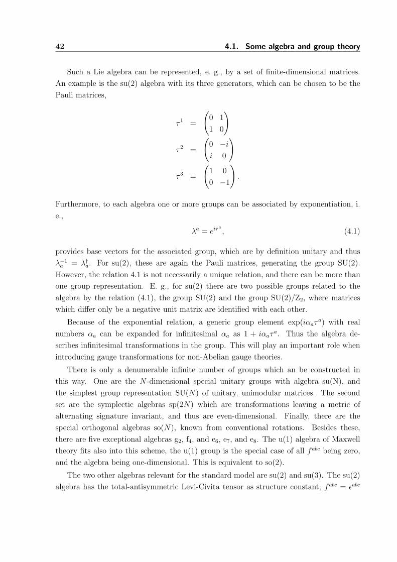
42 4.1. Some algebra and group theory

Such a Lie algebra can be represented, e. g., by a set of finite-dimensional matrices.

An example is the su(2) algebra with its three generators, which can be chosen to be the

Pauli matrices,

τ 1 =

(

0 1

1 0

)

τ 2 =

(

0 −ii 0

)

τ 3 =

(

1 0

0 −1

)

.

Furthermore, to each algebra one or more groups can be associated by exponentiation, i.

e.,

λa = eiτa

, (4.1)

provides base vectors for the associated group, which are by definition unitary and thus

λ−1a = λ†a. For su(2), these are again the Pauli matrices, generating the group SU(2).

However, the relation 4.1 is not necessarily a unique relation, and there can be more than

one group representation. E. g., for su(2) there are two possible groups related to the

algebra by the relation (4.1), the group SU(2) and the group SU(2)/Z2, where matrices

which differ only be a negative unit matrix are identified with each other.

Because of the exponential relation, a generic group element exp(iαaτa) with real

numbers αa can be expanded for infinitesimal αa as 1 + iαaτa. Thus the algebra de-

scribes infinitesimal transformations in the group. This will play an important role when

introducing gauge transformations for non-Abelian gauge theories.

There is only a denumerable infinite number of groups which an be constructed in

this way. One are the N -dimensional special unitary groups with algebra su(N), and

the simplest group representation SU(N) of unitary, unimodular matrices. The second

set are the symplectic algebras sp(2N) which are transformations leaving a metric of

alternating signature invariant, and thus are even-dimensional. Finally, there are the

special orthogonal algebras so(N), known from conventional rotations. Besides these,

there are five exceptional algebras g2, f4, and e6, e7, and e8. The u(1) algebra of Maxwell

theory fits also into this scheme, the u(1) group is the special case of all fabc being zero,

and the algebra being one-dimensional. This is equivalent to so(2).

The two other algebras relevant for the standard model are su(2) and su(3). The su(2)

algebra has the total-antisymmetric Levi-Civita tensor as structure constant, fabc = ǫabc

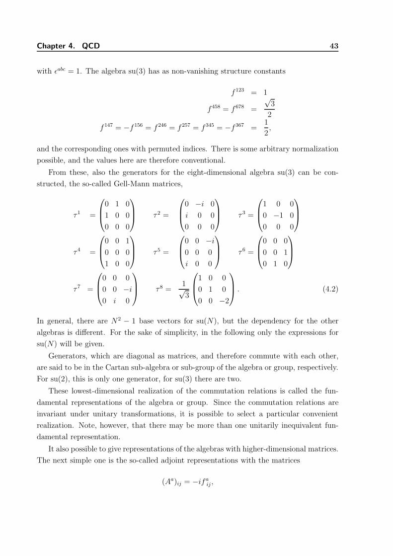
Chapter 4. QCD 43

with ǫabc = 1. The algebra su(3) has as non-vanishing structure constants

f 123 = 1

f 458 = f 678 =

√3

2

f 147 = −f 156 = f 246 = f 257 = f 345 = −f 367 =1

2,

and the corresponding ones with permuted indices. There is some arbitrary normalization

possible, and the values here are therefore conventional.

From these, also the generators for the eight-dimensional algebra su(3) can be con-

structed, the so-called Gell-Mann matrices,

τ 1 =

0 1 0

1 0 0

0 0 0

τ 2 =

0 −i 0

i 0 0

0 0 0

τ 3 =

1 0 0

0 −1 0

0 0 0

τ 4 =

0 0 1

0 0 0

1 0 0

τ 5 =

0 0 −i0 0 0

i 0 0

τ 6 =

0 0 0

0 0 1

0 1 0

τ 7 =

0 0 0

0 0 −i0 i 0

τ 8 =

1√3

1 0 0

0 1 0

0 0 −2

. (4.2)

In general, there are N2 − 1 base vectors for su(N), but the dependency for the other

algebras is different. For the sake of simplicity, in the following only the expressions for

su(N) will be given.

Generators, which are diagonal as matrices, and therefore commute with each other,

are said to be in the Cartan sub-algebra or sub-group of the algebra or group, respectively.

For su(2), this is only one generator, for su(3) there are two.

These lowest-dimensional realization of the commutation relations is called the fun-

damental representations of the algebra or group. Since the commutation relations are

invariant under unitary transformations, it is possible to select a particular convenient

realization. Note, however, that there may be more than one unitarily inequivalent fun-

damental representation.

It also possible to give representations of the algebras with higher-dimensional matrices.

The next simple one is the so-called adjoint representations with the matrices

(Aa)ij = −ifaij ,

44 4.1. Some algebra and group theory

which are three-dimensional for su(2) and eight-dimensional for su(3). There are cases in

which the fundamental and the adjoint representation coincide. This can be continued to

an infinite number of further representations, which will not be needed here.

Further useful quantities are given by the Dynkin index TR for an arbitrary represen-

tation R (being e. g. τ or A)

trRaRb = δabTR,

and the Casimirs CR

RaijR

ajk = δikCR,

being for su(N) (N2 − 1)/(2N) for the fundamental representation and N for the adjoint

representation.

To perform a path-integral quantization of a theory involving Lie algebras, it will be

necessary to integrate over a group. This can be done using the Haar measure, defined for

group elements g = exp(θaτa) as

dg = I(θ)ΠNa=1dθ

a,

where I is the integral measure. The Haar measure is invariant under a variable transfor-

mation using a different group-element, i. e., for g → gg′ with an arbitrary different, but

fixed, group element g′ no Jacobian appears. This replaces the translational invariance of

the measure of ordinary integrals. Furthermore, the Haar measure is defined such that

∫

G

dg = 1,

i. e., an integral over the complete group yields unity. The measure I can be shown to be

I(θ) =1

VGdetM

g−1 ∂g

∂θa= iτ bM ba (4.3)

VG =

∫

G

detMΠNa=1dθ

a

where the second line is an implicit definition, and VG is the appropriate normalization

function.

As an example, group elements of SU(2) can be written as

g = eiθaτa

2 =

(

cos η12+ i sin η1

2cos η2 ie−iη3 sin η1

2sin η2

ieiη3 sin η12sin η2 cos η1

2− i sin η1

2cos η2

)

, (4.4)

Chapter 4. QCD 45

where the three-dimensional vector θa with maximum length of 2π due to the periodicity

of the exponential has been decomposed into polar coordinates with η1 and η3 ranging

from 0 to 2π and η2 to π. Using the implicit definition (4.3), this yields the Haar measure

for SU(2)

dg =4

VGsin2 η1

2dη1 sin η2dη2dη3,

and the group volume VG has a value of 16π2.

This completes the required group theory necessary to describe the standard model.

4.2 Yang-Mills theory

This permits now to formulate QCD. In a first step, this will require the introduction of a

gauge theory being a tensor product of a vector field times a Lie algebra, a so-called Yang-

Mills theory. This will be done here for arbitrary gauge groups, though the dimension

of the algebra will be referred to as colors. After that, the algebra will be specialized to

the ones needed in the standard model, su(2) and su(3), with the group representations

SU(2)/Z2 and SU(3)/Z3. However, the division by Zi will not be relevant in perturbation

theory.

The replacement is rather direct. In the Maxwell theory, the gauge fields were a

product of the (trivial) generator of u(1), being 1, and the gauge field Aµ. Thus, for a

theory including a Lie algebra, a so-called Yang-Mills theory, just the generator will be

replaced by the generators of the group, i. e., the gauge fields will be given as

Aµ = Aaµτa

with the generators τa being in some representation of the gauge algebra. Hence, there

are dimG gauge fields in a Yang-Mills theory, which are essentially algebra-valued. In the

case of the standard model, the representation is the fundamental one, though this is not

specified for most of the following.

It then remains to construct a gauge-invariant action for Yang-Mills theory. This is

again an axiomatic process, which can be motivated by various geometric arguments, but

in the end remains a postulate.

Since the gauge field is now Lie-algebra-valued, so will be any gauge transforma-

tion function, τaωa(x), from which the group-valued unitary gauge transformation G =

exp igτaωa is obtained. The gauge transformation acts now on the gauge fields as

Aµ → GAµG−1 +G∂µG

−1, (4.5)

46 4.2. Yang-Mills theory

which in infinitesimal form reads for the gauge fields Aaµ

Aaµ → Aaµ +Dabµ ωb

Dabµ = δab∂µ − gfabcA

cµ,

where Dabµ is the covariant derivative in the adjoint representation of the gauge group.

There are two remarkable facts about this. One the one hand, there appears an arbitrary

constant g in this relation. This constant will later turn out to take the place of the

conventional electric charge as the coupling constant of Yang-Mills theory. The second

is that the transformation is no longer linear, but there appears a product, even in the

infinitesimal case, of the gauge field and the gauge transformation function ωa. This

non-linearity gives rise to all kind of technical complications.

This more lengthy expression requires also a change of the field-strength tensor, to

obtain a gauge-invariant theory in the end. The field strength tensor of Yang-Mills theory

is

Fµν = ∂µAν − ∂νAµ − ig[Aµ, Aν ] = F aµντa = (∂µA

aν − ∂νA

aµ + gfabcAbµAcν)τa.

There are two more remarkable facts about this field strength tensor. One is that it is no

longer linear in the gauge fields, but that there appears an interaction term: Gauge fields

in a Yang-Mills theory interact with each other, and the theory is even without matter

non-trivial. Furthermore, the appearance of g confirms its interpretation as a coupling

constant. The second is that a quick calculation shows that this expression is not gauge-

invariant, in contrast to Maxwell theory. The reason is the non-commutativity of the

algebra-valued gauge fields.

However, the combination

tr(FµνFµν) = F a

µνFµνa

is. Thus, in analogy to Maxwell theory, the Lagrangian

L = −1

4tr(FµνF

µν) = −1

4F aµνF

µνa ,

defines a suitable gauge-invariant object, which defines Yang-Mills theory. Though it looks

simple at first, it is a highly non-trivial theory, as it includes the interaction of three and

four gauge bosons.

Another consequence of the gauge-variance of the field strength tensor is that color-

electric and color-magnetic fields are gauge-variant as well, and they can thus not be

measured: Yang-Mills theories do not manifest themselves as observable fields nor as

observable color waves. From this follows also that color charge is gauge-variant and thus

Chapter 4. QCD 47

not observable, in contrast to electric charge. The only type of gauge-invariant observables

in Yang-Mills theory are bound-states, the aforementioned glueballs, and the interactions

and behaviors of these glueballs. However, after fixing a gauge, it is of course possible to

make statements also about the gauge bosons, and even use experiments to indirectly say

something about the properties of gauge bosons in a particular gauge.

4.3 QCD

It is straightforward to include also fermions (or scalars) in a Yang-Mills theory. To do

this, it is necessary to select a representation for the matter field ψ. They then receive an

additional index i, which counts the dimensionality of representation of the gauge group:

this enumerates the color. The matter fields, in contrast to the gauge fields, act in the

group, and not in the algebra.

In analogy to QED they then transform under gauge transformations as

ψi → (Gψ)i = Gijψj = exp (−igτaωa)ij ψj ,

which is therefore a group transformation. The generator τa is now in the chosen repre-

sentation of the matter-fields.

To construct a gauge-invariant action, the covariant derivative for minimal coupling

has to include this as well, and it reads now

(Dµ)ij = δij∂µ + igAaµ(τa)ij.

with again the generators τa in the representation of the matter fields.

QCD contains the six quark flavors, counted by a further index f of quarks, which are

all in the fundamental representation of the gauge group, which turns out to be SU(3)/Z3

by comparison to experiment. This also explains the difference of gluon and quark colors:

The respective indices belong to different representations of the gauge group.

Thus, the Lagrangian of QCD reads

LQCD = −1

4F aµνF

aµν +

∑

f

ψfi (iγµDij

µ −mf)ψfj , (4.6)

where the generators τa appearing in the covariant derivative are the Gell-Mann matrices

(4.2). Here the tree-level mass of the quarks mf has been incluced explicitly, as the Higgs

effect in calculations concentrating on QCD phenomena is usually approximated by such

tree-level masses.

It should be noted that the coupling appearing in the covariant derivatives is the same

for all flavors. The difference in color comes only from the different group indices, e. g.,

48 4.4. Quantization of Yang-Mills theories

index i = 1 is red, and so on. This is in contradistinction to QED, where the different

flavors (may) have a different charge. The reason for this is the non-linearity of the gauge

transformation of the gauge field (4.5). For the non-linear part to cancel in the covariant

derivative of the matter fields, the value of the gauge coupling g for the gauge fields and all

matter fields has to be the same, a fact which is known as coupling universality. Otherwise,

the theory would not be gauge-invariant. This is not the case for QED, since there is no

non-linear part of the gauge field gauge transformation in QED.

4.4 Quantization of Yang-Mills theories

The quantization of Yang-Mills theory follows essentially the same steps as for QED.

However, the non-linearity will introduce further complications, and will necessitate the

introduction of further auxiliary fields, the so-called ghost fields, to obtain a description

in terms of a local quantum field theory, at least in perturbation theory. For QCD, it is

as convenient as for QED to not include the matter fields in the gauge condition, so this

will be restricted again to covariant gauges.

First of all, since the gauge transformations (4.5) leave the action invariant, there are

again flat directions similar to QED, thus giving the same reason to implement a gauge-

fixing procedure. However, in the following only the procedure for the perturbative case

will be discussed. The extension to the non-perturbative case is far from obvious for

non-Abelian gauge theories, due to the presence of the so-called Gribov-Singer ambiguity,

which will not be treated here. In case of Yang-Mills theory, some possibilities exist to

resolve this issue, though a formal proof is yet lacking.

The first step is again to select a gauge condition, but this time one for every gauge

field, Ca[Aaµ, x] = 0, e. g. again the the Landau gauge1 Ca = ∂µAaµ. The next steps are then

the same as for QED, only keeping in mind to drag the additional indices alongside, and

that the integration over gauge transformations is now performed using the Haar measure.

This continues until reaching the expression

Z =

∫

DG∫

DAaµ∆[Aaµ]δ(Ca[Aaµ]) exp(iS[A

aµ])

in which for QED ∆ could essentially be absorbed in the measure. For non-Abelian gauge

1For simplicity, here only gauge conditions linear in the group indices are used. Of course, in general

gauge conditions can also depend on gluon fields with a different index than their own.

Chapter 4. QCD 49

theories, this is not possible. For a non-Abelian gauge field, the function ∆ is given by2

∆[Aaµ] =

(

detδCa[Aµ, x])

δθb(y)

)

Ca=0

= detMab(x, y). (4.7)

with the non-Abelian Faddeev-Popov operator Mab.

A more explicit expression is again obtained using the chain rule

Mab(x, y) =δCa(x)

δθb(y)=

∫

d4zδCa(x)

δAcµ(z)

δAcµ(z)

δθb(y)

=

∫

d4zδCa(x)

δAcµ(z)Dcbµ δ(y − z) =

δCa(x)

δAcµ(y)Dcbµ (y).

To proceed further, a choice of Ca is necessary, which will again be covariant gauges,

selected by the condition Ca = Da + Λa(= ∂µAaµ + Λa) for some arbitrary functions Λa.

The path integral then takes the form

Z =

∫

DΛaDAaµ exp(

− i

2ξ

∫

d4xΛaΛa

)

detMδ(C) exp(iS)

=

∫

DAaµ detM exp

(

iS − i

2ξ

∫

d4xDaDa

)

, (4.8)

for a Gaussian weight, and the δ-function has been used in the second step. As the

determinant of an operator is a highly non-local object, the current expression is unsuited

for most calculations.

This non-locality can be recast, using auxiliary fields, as an exponential. Using the

rules of Grassmann numbers it follows immediately that

detM ∼∫

DcaDca exp(

−i∫

d4xd4yca(x)Mab(x, y)cb(y)

)

, (4.9)

where the auxiliary Faddeev-Popov ghost and antighost fields c and c are Grassmann-

valued scalar fields. Since these are just auxiliary fields, this is not at odds with the

spin-statistics theorem. The fields are in general gauges not related, but may be so in

particular gauges. This is, e. g., the case in Landau gauge where there exists an associated

symmetry. If the condition Da is local in the fields, the Faddeev-Popov operator will be

proportional to δ(x− y), and this ghost term will become local.

It is furthermore often useful to introduce an additional auxiliary field, the Nakanishi-

Lautrup field ba. This is obtained by rewriting

exp

(

− i

2ξ

∫

d4xDaDa

)

∼∫

Dba exp(

i

∫

d4x

(

ξ

2baba + baD

a

))

.

2This determinant can be zero outside perturbation theory. This far more involved case will not be

treated here where the matrix in perturbation theory is almost the unit matrix.

50 4.5. BRST and asymptotic states

Upon using the equation of motion for the b field, the original version is recovered.

The final expression then reads

Z =

∫

DAaµDbaDcaDca exp(

iS +

∫

d4x

(

ξ

2baba + baD

a

)

−∫

d4xd4yca(x)Mab(x, y)cb(y)

)

.

Choosing the gauge Da = ∂µAaµ = 0, this takes the form

Z =

∫

DAaµDbaDcaDca exp(

iS + i

∫

d4x

(

ξ

2baba + ba∂µA

µa

)

− i

∫

d4xca∂µDabµ c

b

)

.

Furthermore, the ever-so popular Landau gauge corresponds to the limit ξ → 0, as this is

corresponding to the case where all of the weight of the weight-function is concentrated

only on the gauge copy satisfying ∂µAaµ = 0. However, in principle this limit may only be

taken at the end of the calculation.

To return to QED, it is sufficient to notice that in this case

Dabµ φ

b → ∂µφ,

and thus the ghost term takes the form

−i∫

d4xca∂2ca.

Hence, the ghosts decouple, and will not take part in any dynamical calculations. However,

their contribution can still be important, e. g., in thermodynamics. The decoupling of the

ghost is not a universal statement. Choosing a condition which is not linear in the gauge

fields will also in an Abelian theory introduce interactions. Furthermore, from the sign of

this term it is also visible that the kinetic term of the ghosts has the wrong sign compared

to ordinary scalars, a sign of their unphysical spin-statistic relation.

This program can be performed in a much more formal and general way, the so-called

anti-field method, and also using canonical quantization. Both are beyond the scope of

this lecture.

4.5 BRST and asymptotic states

As stated, the gauge fields themselves are no longer physical in a Yang-Mills theory. It thus

requires some other method to identify physical degrees of freedom, and a more general

construction of the physical state space is required.

A possibility to establish the physical state space is by use of the BRST (Becchi-Rouet-

Stora-Tyutin) symmetry, which is a residual symmetry after gauge-fixing. Perturbatively,

it permits to separate physical from unphysical fields. In the so-called Kugo-Ojima con-

struction it is attempted to extend this construction beyond perturbation theory, though

whether this is possible has not yet been settled.

Chapter 4. QCD 51

4.5.1 BRST symmetry

The starting point for the discussion is the gauge-fixed Lagrangian with Nakanishi-Lautrup

fields included

L = −1

4F aµνF

µνa +

ξ

2baba + baDa −

∫

d4zua(x)δDa

δAcνDcbν ub(z).

Herein the gauge condition is encoded in the condition Ca = 0. Furthermore, matter fields

are ignored, as they will not alter the discussion qualitatively. These contributions will be

reinstantiated later.

This Lagrangian furnishes a global symmetry, as it is invariant under the transforma-

tion δB defined as

δBAaµ = λDab

µ ub = λsAaµ

δBua = −λ g

2fabcubuc = λsua

δBua = λba = λsua

δBba = 0 = λsba.

Herein, λ is an infinitesimal Grassmann number, i. e., it anticommutes with the ghost

fields.

As a consequence, the so-called BRST transformation s has to obey the generalized

Leibnitz rule

s(FG) = (sF )G+ (−1)Grassmann parity of FFsG.

The Grassmann parity of an object is 1 if it is Grassmann odd, i. e. contains an odd

number of Grassmann numbers, and 0 otherwise.

Showing the invariance is simple for the classical Lagrangian, as the transformation

for the gauge boson is just an ordinary gauge transformation with gauge parameter λua,

which is an ordinary real function.

That the remaining gauge-fixing part of the Lagrangian is invariant under a BRST

transformation can be seen as follows. The quadratic term in ba is trivially invariant. The

second term from the gauge-fixing part transforms for a linear gauge condition Da as

s(baDa) = ba∫

d4yδDa

δAbµsAbµ = ba

∫

d4yδDa

δAbµDbcµ uc.

To determine the transformation of the ghost-part, there are four components on which

the transformation acts. The first is when s acts on the anti-ghost. This yields

−s(ua(x))∫

d4zδDa

δAbνDbcν uc(z) = −ba

∫

d4zδDa

δAbνDbcν uc(z).


It therefore precisely cancels the contribution from the second part of the gauge-fixing

term.

The next is the action on the gauge-fixing condition,∫

d4ys

(

δDa

δAbν(y)

)

Dbcν uc =

∫

d4yd4zδDa

δAbν(y)δAdρ(z)

(sAdρ(z))Dbcν uc(y)

=

∫

d4yd4zδDa

δAbν(y)δAdρ(z)

Ddeρ ue(z)D

bcν uc(y) = 0.

In linear gauges, like the covariant gauges, it immediately vanishes since the second deriva-

tive of the gauge condition is zero. In non-linear gauges, this becomes more complicated,

and in general requires the exploitation of various symmetry properties, depending on the

actual gauge condition.

The two remaining terms can be treated together as

s(Dabµ ub) = ∂µsu

a − gfabc ((sAcµ)ub + Acµsub)

= −g2∂µ(f

abcubuc)− gfabcDcdµ udub − gfabcfbdeA

cµu

due

=g

2fabc (∂µ(ubu

c)− 2ub∂µuc − 2g(f cdeAeµudub + gf de

b Acµudue)).

The first two terms cancel each other, after adequate relabeling of indices. The last two

terms can be rearranged by index permutation such that the Jacobi identity can be used

so that they vanish as well,

=g

2fabc(ub∂

µuc + (∂µub)uc − 2ub∂µuc)

+g(fabcf decAµeudub + fabcf decA

µeudub + fabcf decA

µb udue)

= g(fabcf decAµeudub + fadcf ebcAµeudub + faecf dbcAµeudub)

= g(fabef cde + facef dbe + fadef bce)Aµcudub = 0,

for which a number of index rearrangements and relabellings are necessary, taking always

the Grassmannian nature of the ghost duly into account. Hence, indeed the gauge-fixed

Lagrangian is BRST-invariant.

An amazing property of the BRST symmetry is that it is nil-potent, i. e., s2 = 0. This

follows immediately from a direct application. The previous calculation already showed

that

0 = s(Dabµ u

b) = s2Aaµ.

It is trivial for the anti-ghost and the auxiliary ba field by construction. For the ghost it

immediately follows by

s2ua ∼ s(fabcubuc) ∼ fabcf deb udueuc − fabcf de

c ubudue = fabcf deb (udueuc + ucudue) = 0.

Chapter 4. QCD 53

the last step is not trivial, but follows from the fact that the ghost product is Grassmannian

in nature, and only non-zero if all three indices are different, and thus behaves as an anti-

symmetric tensor ǫcde.

There is even more possible. It holds that the gauge-fixing part of the Lagrangian can

be written as

Lf = s

(

ua(

ξ

2ba +Da

))

=ξ

2baba + baDa + ua

∫

d4yδDa

δAbµ(y)Dbcµ ub(y).

Hence, the gauge-fixing part of the Lagrangian is BRST-invariant, since s2 = 0. This can

be generalized to other gauge conditions by adding arbitrary BRST-exact terms s(uaFa)

with F a arbitrary to the Lagrangian. The factor of u is necessary to compensate the ghost

of the BRST transformation, since any term in the Lagrangian must have a net number

of zero ghosts. This extension leads to the so-called anti-field formalism for gauge-fixing.

This will not be pursued further here.

The BRST transformation for matter fields also take the form of a gauge transformation

with the parameter λua. Therefore, all matter Lagrangian contributions automatically

satisfy invariance under a BRST transformation. For a fermionic or bosonic matter field

φ in representation τa it takes the form

δBφi = λiguaτ ija φj

s2φi = igτ ija s(uaφj) = igτ ija

(g

2fabcubucφj + iguaubτ

bjkφ

k)

∼ g2

τa, τ bij

uaubφj = 0,

where in the second-to-last step the relation between structure constants and generators

has been used backwards, permitting to combine both terms into the symmetric anti-

commutator. The combination with the anti-symmetric ghost product yields then zero.

4.5.2 Constructing the physical state space

The following discussion shows how to explicitly construct the state space using BRST

symmetry. It extends thereby the Gupta-Bleuler construction of QED, and it can be

directly extended to include also matter fields.

The first concept in constructing the physical state space is the presence of states which

do not have a positive norm. The simplest example is already given in Maxwell theory.

Choose, e. g., Feynman gauge, i. e. ξ = 1. The corresponding propagator is then given by

Gaussian integration as

< A†µ(x)Aν(y) >= δabgµν

∫

d4p

(2π)4eip(x−y)

p2 + iǫ= −δabgµν

∫

d3p

2(2π)3|~p|e−ipi(x−y)i .


The norm of a state

Ψ(x) =

∫

d4xf(x)A0(x)|0 >=∫

d4xd4p

(2π)4eip0x0−pixif(p)A0(x)|0 >,

with f(x) an arbitrary weight function, created from the vacuum by the operator Aµ then

reads

|Ψ|2 =∫

d4x

∫

d4y < A†0(x)A0(y) > f †(x)f(x) = −

∫

d3p

2|~p|f†(p)f(p) < 0.

Hence, there are negative (and zero) norm states present in the state space. These cannot

contribute to the physical state space, or otherwise the probability interpretation of the

theory will be lost. Or at least, it must be shown that the time evolution is only connecting

physical, i. e. with positive definite norm, initial states to physical final states.3

That they indeed do not contribute can be shown using the BRST symmetry. In fact,

it will be shown that

QB|ψ >phys = 0, (4.10)

[QB, ψ]± = sψ.

will be sufficient to define the physical state space, where the second line defines the BRST

charge QB. The ± indicate commutator or anticommutator, depending on whether ψ is

bosonic (commutator) or fermionic (anticommutator). The BRST charge QB can also be

defined from the Noether current. It is given by

QB =

∫

d3x

(

baDab0 ub − ua∂0b

a +1

2gfabcubuc∂0ua

)

.

It is fermionic. Since s2 = 0 it directly follows that Q2B = 0 as well.

The BRST charge has evidently a ghost number of 1, i. e., the total number of ghost

fields minus the one of anti-ghosts is 1. This ghost number, similarly to fermion number,

is actually a conserved quantum number of the theory. It is due to the invariance of the

Lagrangian under the scale transformation

ua → eαua

ua → e−αua,

3The precise characterization of what is a final state beyond perturbation theory is open. One pos-

sibility, discussed before, is a non-perturbative extension of the construction to follow. Another one

characterizes all physical states by the necessary condition to be invariant under renormalization - after

all, physics should be independent of the scale at which it is measured. However, whether this condition

is sufficient, in particular beyond perturbation theory, is also not clear. Bound states with non-zero ghost

number, e. g., may also possess this property, though may not be a viable physical state.

Chapter 4. QCD 55

with real parameter α. Note that such a scale transformation is possible since ua and ua

are independent fields. Furthermore for a hermitiean Lagrangian the relations

u† = u

u† = −u

hold. As a consequence, also the BRST transformation and charge have ghost number 1

and are Hermitiean.

Since the Lagrangian is invariant under BRST transformation, so is the Hamiltonian,

and therefore also the time evolution and thus the S-matrix,

[QB, H ] = 0

[QB, S] = 0.

Hence, if in fact the BRST symmetry is manifest4, and the condition (4.10) defines the

physical subspace that is already sufficient to show that physical states will only evolve

into physical states. It remains to seen what kind of states satisfy (4.10).

Because the BRST charge is nilpotent the state space can be separated in three sub-

spaces:

• States which are not annihilated by QB, V2 = |ψ > |QB|ψ > 6= 0.

• States which are obtained by QB from V2, V0 = |φ > ||φ >= QB|ψ >, |ψ > ǫV2.As a consequence QBV0 = 0.

• States which are annihilated by QB but do not belong to V0, V1 = |χ > |QB|χ >=0, |χ > 6= QB|ψ >, ∀|ψ > ǫV2.

The states in V2 do not satisfy (4.10), and therefore would not be physical. The union of

the two other states form the physical subspace.

Vp = V0 ∪ V1.

It is this subspace which is invariant under time evolution. It is not trivial to show that

all states in this space have positive semi-definite norm, but this is possible. This fact will

be used here without proof. However, all states in V0 have zero norm, and have no overlap

with the states in V1,

< φ|φ > =< φ|QB|ψ >= 0

< φ|χ > =< ψ|QB|χ >= 0.

4The consequences of a not manifest BRST are far from trivial, and the non-perturbative status of

BRST symmetry is still under discussion, though there is quite some evidence that if it can be defined it

is well defined. But how to define it is not finally settled.


Since matrix elements are formed in this way the states in V0 do not contribute, and every

state in Vp is thus represented by an equivalence class of states characterized by a distinct

state from V1 to which an arbitrary state from V0 can be added, and thus a ray of states.

Therefore, the physical Hilbert Hp state can be defined as the quotient space

Hp = Vp/V0 =KerQB

ImQB,

the so-called cohomology of the operator QB. Therefore, all states in Hp have positive

norm, provided that the states in V1 have.

To define the theory in the vacuum, use can be made of asymptotic states, in pertur-

bation theory usually known as in and out states. A corresponding physical asymptotic

states ψap must therefore obey

sψap = 0.

In the following, the classification of the fields will be done in this form for perturbation

theory. In this case, this will finally amount to discarding essentially all composite fields.

Beyond perturbation theory, this is no longer possible, as cluster decomposition in general

no longer holds in gauge theories. How to proceed beyond perturbation theory is therefore

not completely understood.

To obtain the asymptotic fields, start with the BRST variation of a given Green’s

functions. Asymptotic fields are defined to be the pole-part of the asymptotic field. To

obtain these, start with the formula

< T (sψi)ψi1 ...ψin >=< T (sψi)ψk >< Tψkψi1 ...ψin > .

In this case, the indices i sum all space-time and internal indices and T is the time-ordering.

Essentially, a one has been introduced. Since in perturbation theory all interactions are

assumed to cease for asymptotic states, the BRST transformation become linear in the

fields

sψi → sψai = Cikψak .

Furthermore, by comparison with the previous calculation, the coefficients can be defined

as

Cik =< T (sψi)ψk >=1

Z[0]

iδ2

δJsψiδJψk

Z[J ]

at least asymptotically. Note that the source coupled to sψi is necessarily the one for a

composite operator. Since in this case the Green’s functions will be dominated by the

on-shell (pole) part, only those coefficients will be relevant where sψi and ψk have the

same mass.

Chapter 4. QCD 57

As a consequence, this condition reads

Jpi sψapi = Jpi

1

Z[0]

iδ2Z[J ]

δJsψiδJψk

ψak = 0,

since the BRST-variation of physical fields vanish.

The interesting question is then the form of these asymptotic propagators appearing.

In case of the gauge field

sAlaµ (x) =

∫

d4yRlmµ (x, y)uma(y), (4.11)

where the index a stands for asymptotic. That only u appears is due to the fact that the

ghost is the parameter of the BRST transformation. The propagator then has the form

Rabµ =< T (sAaaµ )ub >= − < TAaaµ su

b > .

The later identity is correct, since

s(AB) = (sA)B + (−1)gBAsB (4.12)

and the fact that a physical vacuum expectation value for any pure BRST variation, s(AB)

vanishes, < s(AB) >= 0. It then follows further

− < TAaµbb >= −1

ξ< TAaµC

b >=1

ξ< TAaµA

cν > φνbc =

1

ξDacµνφ

νbc (4.13)

where it was assumed in the second-to-last step that the gauge-fixing condition Ca is linear

in the field, Ca = φbcν Aν , and the appearance of partial derivatives has been compensated

for by a change of sign. This is therefore a statement for all contributions not-orthogonal

to φbcν .

Now, because of Lorentz and (global) gauge invariance, it must be possible to rewrite

Rabµ = δab∂µR.

Therefore, asymptotically

δab∂µR =1

ξDacµνφ

νcb = − < TAaµb

b > (4.14)

must hold. The gluon propagator is asymptotically the free one. The right-hand side

equals precisely the mixed propagator of the free Aµ and ba field. This one is given by

δab∂µδ(x − y), as can be read off directly from the Lagrangian. Therefore, R = δ(x − y)

to obtain equality. Reinserting this into (4.11) yields

sAaaµ = ∂µua.


For the ghost the asymptotic BRST transformation vanishes, since its BRST transform is

of ghost number 2. There is no single particle state with such a ghost number. The BRST

transformed of the anti-ghost field is already linear, yielding

sAaaµ = ∂µua

suaa = 0

suaa = baa

sbaa = 0,

for the full list of asymptotic BRST transformed fields. Unsurprisingly, these are exactly

the BRST transformations of the free fields.

From this follows that the longitudinal component of Aµ, since ∂µ gives a direction

parallel to the momentum, is not annihilated by s, nor is the anti-ghost annihilated by

the BRST transformation. They belong therefore to V2. The ghost and the Nakanishi-

Lautrup field are both generated as the results from BRST transformations, and therefore

belong to V0. Since they are generated from states in V2 it is said they form a quartet with

parent states being the longitudinal gluon and the anti-ghost and the daughter states being

the ghost and the Nakanishi-Lautrup field. Therefore, these fields not belonging to the

physical spectrum, are said to be removed from the spectrum by the quartet mechanism.

Note that the equation of motion for the field ba makes it equivalent to the divergence of

the gluon field, which can be taken to be a constraint for the time-like gluon. Therefore,

the absence of the Nakanishi-Lautrup field from the physical spectrum implies the absence

of the time-like gluon. Finally, the transverse gluon fields are annihilated by the BRST

transformation but do not appear as daughter states, they are therefore physical. In

general gauges, the second unphysical degree of freedom will be the one constrained by the

gauge-fixing condition to which ba is tied, while the two remaining polarization directions,

whichever they are, will be belonging to V1.

Of course, the gauge bosons can not be physical, since they are not gauge-invariant.

Therefore, their removal from the spectrum must proceed by another mechanism, which

is therefore necessarily beyond perturbation theory. A proposal for a similar construction

also applying to the gauge bosons has been given by Kugo and Ojima, though its validity

has not yet satisfactorily been established.

The introduction of fermions (or other matter) fields ψ follows along the same lines. It

turns out that all of the components belong to V1, i. e., sψ = 0, without ψ appearing on

any right-hand side, and therefore all fermionic degrees of freedom are perturbatively phys-

ically. This can be directly seen as their gauge, and consequently BRST, transformation

Chapter 4. QCD 59

is

δψa = iguaτaijψj ,

and hence its free-field (g = 0) result is sψai = 0. This is expected, since no asymptotic

physical bound-state with ghost and fermion number one exists.

Similar as for the gauge boson, this cannot be completely correct, and has to change

non-perturbatively.

Chapter 5

Electroweak interactions and the

Higgs

The so-called electroweak sector of the standard model is actually a combination of several,

closely related ingredients. The central element is a Yang-Mills theory with underlying

gauge algebra su(2), the weak isospin theory. This theory is coupled to a Higgs field,

which spontaneously condenses, and thereby provides mass to the gauge bosons. Both

fields, the weak isospin gauge bosons and the Higgs, couple to the matter fields of the

standard model, where parity is explicitly broken by the coupling of the fermion to the

weak isospin gauge bosons. At the same time, the Higgs boson provides the mass to the

standard model fermions.

As if this triangle of interactions would not be messy enough, the electroweak sector

is also the staging ground for two independent mixing effects. One gives the electroweak

sector its name: The weak gauge bosons and the photons of QED mix, which gives charge

to some of the weak gauge bosons. The second mixing appears in the matter sector, where

the two CKM matrices modify the coupling of the now electroweak gauge bosons to the

matter fields.

All of these effects will be introduced step-by-step in the following, but it is simpler to

start directly with including the mixing effects.

5.1 Assigning the quantum numbers

The basic structure of the weak interactions is a su(2) Yang-Mills theory representing the

weak isospin sector and a u(1) Abelian theory representing a would-be QED sector. As

noted before, the weak isospin sector is parity violating. The important point is that both

sectors mix. This has to be taken into account when assigning the charge structure for

60

Chapter 5. Electroweak interactions and the Higgs 61

this sector of the standard model.

To identify the charge structure, the experimental fact is useful that the weak inter-

actions provide transitions of two types. One is a charge-changing reaction, which acts

between two gauge eigenstates. In case of the leptons, these charge eigenstates are almost

(up to a violation of the order of the neutrino masses) exactly a doublet - e. g., the electron

and its associated electron neutrino, as well as a pairing of an up-type quark (up, charm,

top with electric charge +2/3) and a down-type quark (down, strange, bottom with electric

charge -1/3). Since the electric charge of the members of the doublets differ by one unit,

the off-diagonal gauge bosons, the W, must carry a charge of one unit. Furthermore, su(2)

has three generators. The third must therefore be uncharged, as it mediates interactions

without exchanging flavors: It is the Cartan of the su(2) group.

Furthermore, this implies that the left-handed fermions have two different charges

under the weak interactions, which assigns them to the fundamental representation of the

su(2) gauge group. This quantum number distinguishing the two eigenstates of a doublet

is called the third component of the weak isospin t, and will be denoted by t3 or I3W .

However, the weak gauge bosons are charged. Therefore, ordinary electromagnetic

interactions have to be included somehow. Since ordinary electromagnetism has a one-

dimensional representation, its gauge algebra is the Abelian u(1). The natural ansatz for

the gauge group of the electroweak interactions is thus the gauge group SU(2)×U(1)1.

With this second factor-group comes a further quantum number, which is called the hy-

percharge y. The ordinary electromagnetic charge is then given by

eQ = e(

t3 +y

2

)

. (5.1)

Thus, the ordinary electromagnetic interaction must be somehow mediated by a mixture

of the neutral weak gauge boson and the gauge boson of the U(1). This is dictated by

observation: It is not possible to adjust otherwise the quantum numbers of the particles

such that experiments are reproduced. The hypercharge of all left-handed leptons is −1,

while the one of left-handed quarks is y = +1/3.

Right-handed particles are neutral under the weak interaction. In contrast to the

t = 1/2 doublets of the left-handed particle, they belong to a singlet, t = 0. All in all,

the following assignment of quantum numbers for charge, not mass, eigenstates will be

necessary to reproduce the experimental findings:

• Left-handed neutrinos: t = 1/2, t3 = 1/2, y = −1 (Q = 0)

• Left-handed leptons: t = 1/2, t3 = −1/2, y = −1 (Q = −1)

1Actually, the correct choice is SU(2)/Z2×U(1), though this difference is not relevant in perturbation

theory, and therefore neglected here.

62 5.1. Assigning the quantum numbers

• Right-handed neutrinos: t = 0, t3 = 0, y = 0 (Q = 0)

• Right-handed leptons: t = 0, t3 = 0, y = −2 (Q = −1)

• Left-handed up-type (u, c, t) quarks: t = 1/2, t3 = 1/2, y = 1/3 (Q = 2/3)

• Left-handed down-type (d, s, b) quarks: t = 1/2, t3 = −1/2, y = 1/3 (Q = −1/3)

• Right-handed up-type quarks: t = 0, t3 = 0, y = 4/3 (Q = 2/3)

• Right-handed down-type quarks: t = 0, t3 = 0, y = −2/3 (Q = −1/3)

• W+: t = 1, t3 = 1, y = 0 (Q = 1)

• W−: t = 1, t3 = −1, y = 0 (Q = −1)

• Z: t = 1, t3 = 0, y = 0 (Q = 0)

• γ: t = 0, t3 = 0, y = 0 (Q = 0)

• Gluon: t = 0, t3 = 0, y = 0 (Q = 0)

• Higgs: a complex doublet, t = 1/2 with weak hypercharge y = 1. This implies zero

charge for the t3 = −1/2 component, and positive charge for the t3 = 1/2 component

and negative charge for its complex conjugate

This concludes the list of charge assignments for the standard model particles. The Higgs

case, where now four rather than one Higgs are necessary, is special, and will be detailed

in great length below.

Since at the present time the photon field and the Z boson are not yet readily identified,

it is necessary to keep the gauge boson fields for the SU(2) and U(1) group differently, and

these will be denoted by W and B respectively. The corresponding pure gauge part of the

electroweak Lagrangian will therefore be

Lg = −1

4GaµνG

µνa − 1

4FµF

µ

Fµν = ∂µBν − ∂νBµ

Gaµν = ∂µW

aν − ∂νW

aµ + g′fabcW

bµW

cν ,

where g′ is the weak isospin gauge coupling. The fabc are the structure constants of the

weak isospin gauge group, which is just the SU(2) gauge group.


Coupling matter fields to these gauge fields proceeds using the ordinary covariant

derivative, which takes the form

Dµ = ∂µ +ig′

2τaW

aµ +

ig′′y

2Bµ,

where g′′ is the hypercharge coupling constant, which is modified by the empirical factor y.

For fermions, of course, this covariant derivative is contracted with the Dirac matrices γµ.

Precisely, to couple only to the left-handed spinors, it will be contracted with γµ(1−γ5)/2for the W a

µ term and with γµ for the kinetic and hypercharge term, i. e.

γµDµ = γµ(

∂µ +1− γ5

2

ig′

2τaW

aµ +

ig′′y

2Bµ

)

How the weak isospin gauge bosons receive their mass will be discussed next. For this

purpose, the hypercharge gauge bosons will be neglected for now.

5.2 Hiding local symmetries

When coupling the Higgs to a gauge field, the Higgs effect becomes more complicated,

but at the same time also more interesting, than in the case without gauge fields. For

simplicity, start with an Abelian gauge theory, coupled to a single, complex scalar, the

so-called Abelian Higgs model, before going to the full electroweak and non-Abelian case.

This theory has the Lagrangian

L =1

2((∂µ + iqAµ)φ)

+(∂µ + iqAµ)φ− 1

4(∂µAν − ∂νAµ)(∂

µAν − ∂νAµ)

+1

2µ2φ+φ− 1

2

µ2

f 2(φ+φ)2. (5.2)

Note that the potential terms are not modified by the presence of the gauge-field. There-

fore, the extrema have still the same form and values as in the previous case, at least

classically. However, it cannot be excluded that the quartic φ+φAµAµ term strongly dis-

torts the potential. Once more, this does not appear to be the case in the electroweak

interaction, and it will therefore be ignored.

To make the consequences of the Higgs effect transparent, it is useful to rewrite the

scalar field as2

φ(x) =

(

f√2+ ρ(x)

)

exp(iα(x)).

2Note that if the space-time manifold is not simply connected and/or contains holes, it becomes

important that α is only defined modulo 2π. For flat Minkowski (or Euclidean) space, this is of no

importance. However, it can be important, e. g., in finite temperature calculations using the Matsubara

formalism. It is definitely important in ordinary quantum mechanics, where, e. g., the Aharanov-Bohm

effect and flux quantization depend on this.

64 5.2. Hiding local symmetries

This is just another reparametrization for the scalar field, compared to σ and χ previously.

It is such that at ρ = 0 this field configuration will be a classical minimum of the potential

for any value of the phase α. Inserting this parametrization into the Lagrangian (5.2)

yields

L =1

2∂µρ∂

µρ+1

2

(

f√2+ ρ

)2

∂µα∂µα + qAµ

(

f√2+ ρ

)2

∂µα +q2

4AµA

µ

(

f√2+ ρ

)2

−1

4(∂µAν − ∂νAµ)(∂

µAν − ∂νAµ) +1

2µ2

(

f√2+ ρ

)2

− 1

2

µ2

f 2

(

f√2+ ρ

)4

This is an interesting structure, where the interaction pattern of the photon with the radial

and angular part are more readily observable.

Now, it is possible to make the deliberate gauge choice

∂µAµ = −1

q∂2α. (5.3)

This is always possible. It is implemented by first going to Landau gauge and then perform

the gauge transformation

Aµ → Aµ +1

q∂µα

φ → exp(−iα)φ.

This gauge choice has two consequences. The first is that it makes the scalar field real

everywhere. Therefore, the possibility of selecting the vacuum expectation value of φ

to be real is a gauge choice. Any other possibilities, e. g. purely imaginary, would be

an equally well justified gauge choices. This also implies that the actual value of the

vacuum expectation value f of φ is a gauge-dependent quantity. The Lagrangian, up to

gauge-fixing terms, then takes the form

L =1

2∂µρ∂

µρ+q2

4AµA

µ

(

f√2+ ρ

)2

−1

4(∂µAν − ∂νAµ)(∂

µAν − ∂νAµ) +1

2µ2

(

f√2+ ρ

)2

− 1

2

µ2

f 2

(

f√2+ ρ

)4

(5.4)

i. e., the second term has now exactly the form of a screening term, and yields an effective

mass qf/4 for the photon field. Furthermore, if ρ could be neglected, the Lagrangian

would be just

L =q2f 2

8AµA

µ − 1

4(∂µAν − ∂νAµ)(∂

µAν − ∂νAµ),

i. e., the one of a massive gauge field. Together with the gauge condition for Aµ, which links

the longitudinal part of the gauge boson to the now explicitly absent degree of freedom


α, this implies that the field Aµ acts now indeed as a massive spin-1 field. Furthermore,

this Lagrangian is no longer gauge-invariant. This is not a problem, as it was obtained by

a gauge choice. Thus, it is said that the gauge symmetry is hidden. Its consequences are

still manifest, e. g., the mass for the gauge boson is not a free parameter, but given by the

other parameters in the theory. By measuring such relations, it is in principle possible to

determine whether a theory has a hidden symmetry or not.

Colloquial, the hiding of a symmetry is also referred to as the breaking of the symmetry

in analogy with the case of a global symmetry. However, a theorem, Elitzur’s theorem,

actually forbids this to be literally true.

Another theorem, the Goldstone theorem, actually guarantees that a mass will be

provided to each gauge boson associated with one of the hidden generators at the classical

level. This hidden generator is here the phase, which is massless. This masslessness of

the Goldstone boson is actually guaranteed by the Goldstone theorem. Hence, a massless

Goldstone boson is effectively providing a mass to a gauge boson by becoming its third

component via gauge-rotation, and vanishes by this from the spectrum. It is the tri-

linear couplings which provide the explicit mixing terms delivering the additional degree

of freedom for the gauge boson at the level of the Lagrangian. Hence, the number of

degrees of freedom is preserved in the process: In the beginning there were two scalar

and two vector degrees of freedom, now there is just one scalar degree of freedom, but

three vector degrees of freedom. The gauge-transformation made nothing more than to

shift one of the dynamic degrees of freedom from one field to the other. This was possible

due to the fact that both the scalar and the photon are transforming non-trivially under

gauge-transformations.

This can, and will be, generalized below for other gauges. In general, it turns out that

for a covariant gauge there are indeed six degrees of freedom, four of the vector field, and

two from the scalars. Only after calculating a process it will turn out that certain degrees

of freedom cancel out, yielding just a system which appears like having a massive vector

particle and a single scalar.

Note that though the original scalar field φ was charged as a complex field, the radial

excitation as the remaining degree of freedom is actually no longer charged: The coupling

structure appearing in (5.4) is not the one expected for a charged field.

However, the choice (5.3), which is called the unitary gauge, is extremely intransparent

and cumbersome for most actual calculations. The reason is the explicit reappearance of

the phase in further calculational steps in the gauge-fixing term, which has been neglected

in this classical argumentation.

A more convenient possibility, though at the cost of having unphysical degrees of

66 5.3. Quantizing the Abelian-Higgs model

freedom which only cancel at the end, are ’t Hooft gauges. To define this gauge once more

the decomposition

φ = (χ, f + η)

for the scalar field is useful. The Lagrangian then takes the form, up to constant terms,

L = −1

4FµF

µ +(gf)2

2AµA

µ +1

2∂µη∂

µη − µ2η2 +1

2∂µχ∂

µχ− gfAµ∂µχ (5.5)

+2igAµ(χ∂µχ+ η∂µη)− 2g(gf)ηAµAµ − g2(χ2 + η2)AµA

µ − 1

2

µ2

f 2(χ2 + η2)2.

There are a number of interesting observations. Again, there is an effective mass for Aµ,

due to the four-field interaction term. Secondly, only the σ field has a conventional mass

term, the mass-term for the χ field has canceled with the two-field-two-condensate term

from the quartic piece of the potential. Finally, there will be terms of type fAµ∂µχ. This

implies that a photon can change into a χ while moving, with a strength proportional to

the condensate f , and thus mixing between one of the Higgs degrees of freedom and the

photon occurs. Therefore, the photon and this scalar, the would-be Goldstone boson, will

mix. Note finally that though many more interaction terms have appeared, none of them

has any other free parameter, as a consequence of the now hidden symmetry. The only

quantity which looks like a new quantity is the condensate value f , though it is classically

uniquely determined by the shape of the potential. In a quantum calculation, it can also

be determined, but not in perturbation theory, where it remains a fit parameter.

The gauge condition to be used for quantizing this Lagrangian later is then given by

∂µAµ = qfξχ, (5.6)

the so-called renormalizable or ’t Hooft gauge.

The form of the Lagrangian (5.5) already indicates how the weak gauge bosons will

receive their mass next.

5.3 Quantizing the Abelian-Higgs model

In quantized calculations using perturbation theory the ’t Hooft gauge (5.6) is most con-

venient. It is again useful to consider first the simplest example of an (unmixed) Abelian

gauge theory.

Splitting at the classical level the real Higgs doublet as (χ, f + η), where the fields χ


and η fluctuate and f is the expectation value of the vacuum, the Lagrangian reads

L = −1

4FµF

µ +(gf)2

2AµA

µ +1

2∂µη∂

µη − µ2η2 +1

2∂µχ∂

µχ− gfAµ∂µχ

+2igAµ(χ∂µχ+ η∂µη)− 2g(gf)ηAµAµ − g2(χ2 + η2)AµA

µ − 1

2

µ2

f 2(χ2 + η2)2.

The ’t Hooft gauge is exactly the gauge in which the bilinear mixing part is removed from

the Lagrangian. In the Abelian case this is achieved by

C[Aµ, χ] = ∂µAµ + ξ(gf)χ.

Entering this expression into the gauge-fixed Lagrangian (4.8) yields the gauge-fixing term

Lf = − 1

2ξ(∂µAµ + ξ(gf)χ)2 = − 1

2ξ(∂µA

µ)2 + gfAµ∂µχ− ξ

2(gf)2χ2,

where a partial integration has been performed. It should be noted that the gauge-

parameter ξ now enters twice. Once by parametrizing the width of the averaging functional

and once in the gauge condition itself. In principle it would be permitted to choose a dif-

ferent parameter in both cases, but then the mixing terms would not be canceled. In

this gauge the Goldstone field becomes in general massive, exhibiting clearly that the

Goldstone theorem is not applying to the case of a gauge theory.

Furthermore, the limit ξ → 0 corresponds to the case of ordinary Landau gauge with

the mixing term and also the mass-shift for the χ-field due to the gauge-fixing removed

from the Lagrangian. Thus, in the Landau gauge in contrast to other covariant gauges

the Goldstone boson remains massless at tree-level.

The ghost contribution can be determined directly from equation (4.9) using the ex-

pression (4.7) to calculate the Faddeev-Popov determinant. However, it must no be taken

care of the fact that the gauge condition no longer only depends on the gauge field, but

also on the matter fields. Therefore, the expression for the Faddeev-Popov determinant

for a generic gauge condition depending on many fields takes the form

Mab(x, y) =δCa(x)

δθb(y)=

∫

d4z∑

ij

δCa(x)

δωij(z)

δωij(z)

δθb(y).

In this case i counts the field-type, while j is a multi-index, encompassing color, Lorentz

indices etc.. From this, the ghost Lagrangian can be calculated as3

Lg = −c(∂2 + ξ(gf)2 + ξg(gf)η)c.

3Note that a phase transformation mixes real and imaginary parts of a complex field.

68 5.4. Hiding the electroweak symmetry

Thus the ghosts are massive with the same mass as for the Goldstone field. It is this

precise relation which guarantees the cancellation of both unphysical degrees of freedom

in any process. Note that even though the group is Abelian the ghosts no longer decouple

in this gauge. Only in the Landau gauge the then massless ghosts will decouple.

5.4 Hiding the electroweak symmetry

To have a viable theory of the electroweak sector it is necessary to hide the symmetry such

that three gauge bosons become massive, and one uncharged one remains massless. How

this occurs classically will be investigated here. Though this can be of course arranged in

any gauge, it is most simple to perform this in the unitary gauge. Since three fields have

to be massive, this will require three pseudo-Goldstone bosons. Also, since empirically two

of them have to be charged, as the W± bosons are charged, the simplest realization is by

coupling a complex doublet scalar field, the Higgs field, to the electroweak gauge theory

Lh = −1

4FµνF

µν − 1

4GaµνG

µνa +

1

2(Dij

µ φj)+Dµ

ikφk + V (φiφ+

i )

φi =1√2

(

φ1 + iφ2

φ3 + iφ4

)

i

Fµν = ∂µBν − ∂νBµ

Gaµν = ∂µW

aν − ∂νW

aµ + g′fabcWbµWcν

Dijµ = δij∂µ + ig′τ ija W

aµ + δijig′′yBµ

where the field φ is thus in the fundamental representation of the gauge group. Its hyper-

charge will be y = 1, an assignment which will be necessary below to obtain a massless

photon. The potential V can only depend on the gauge-invariant combination φ+φ, and

contains a mass-term and a quartic self-interaction. The mass-term must be again of the

wrong sign (imaginary mass), such that there exists a possibility for the φ field to acquire

a (gauge-dependent) vacuum-expectation value classically.

To work in unitary gauge it is best to rewrite the Higgs field in the form

φ = eiτaαa

2

(

0

v + ρ

)

.

There are now the three αa fields and the ρ field with v(0, 1)T =< φ >. Performing a gauge

transformation such that the phase becomes canceled exactly, and setting ρ = v+η with v

constant makes the situation similar to the one in the Abelian Higgs model. Note that by

a global gauge transformation the component with non-vanishing expectation value can

be selected still at will.


The mass will be made evident by investigating the quadratic interaction terms of the

gauge bosons with the expectation value of the Higgs field, yielding for the quadratic part

of the gauge field Lagrangian

(g′′y)2

2BµB

µv2 +g

′2

2W aµW

µa v

2 + g′yg′′BµW 3µv

2.

There appear mass terms for all four gauge fields, but also a mixing term between the W 3µ

and the Bµ fields. This can be remedied by a change of basis as

Aµ = Bµ cos θW −W 3µ sin θW

Zµ = Bµ sin θW +W 3µ cos θW ,

which are the fields given the name of the photon Aµ and the Z boson Zµ. The mixing

parameter θW is the (Glashow-)Weinberg angle θW , and is given entirely in terms of the

coupling constants g′ and g′′ as

tan θW =g′′

g′

cos θW =g′

√

g′2 + g′′2

sin θW =g′′

√

g′2 + g′′2.

Using the inverse transformations

W 3µ =

Zµ sin θW −Aµ cos θW2 cos θW sin θW

Bµ =Zµ cos θW + Aµ sin θW

2 cos θW sin θW

it is possible to recast the quadratic part of the Lagrangian for the gauge fields, which

becomes

g′2v2

4W µ

±W∓µ +

v2

8(cos θW sin θW )2(Aµ(g

′′ cos θW − g′y sin θW )− Zµ(g′′ cos θW + g′y sin θW ))

2.

Herein the charged W bosons W± have been introduced as

W±µ =

1√2(W 1

µ ∓ iW 2µ),

and their association with an electric charge will become clear in a moment. More impor-

tant is that for the assignment y = 1, as advocated for the Higgs above, the contribution

70 5.4. Hiding the electroweak symmetry

to Aµ drops out, and also there is no longer a mixing term present. Thus, the field Aµ

is massless, and it can be associated with the photon, while the Zµ field is massive. The

masses for the W± and the Z are then

MW =g′v

2

MZ =v

2

√

g′2 + g′′2 =MW

cos θW

and thus the W± are lighter than the Z, and these can be identified with the weak gauge

bosons. The Weinberg angle is close to about 30 degrees, and thus the mass difference is

small, about 15%.

That the W± have an electric charge is now a direct consequence of the self-interaction

of the original W iµ weak isospin bosons: There are interaction vertices which involve all

three gauge fields, e. g.,

W 1νW

ν2 ∂µW

µ3 ∼ 2W+

ν W−ν∂µ

Zµ sin θW − Aµ cos θW2 cos θW sin θW

,

and thus, besides an interaction between the Z and the W±, there is also an interaction

with the photon, which connects a W+ and aW−, just like ordinary matter particles. It is

therefore apt to call the W+ and W− bosons electrically charged, though the precise cou-

pling strength involves the Weinberg angle. Similarly, there are arise interaction vertices

which include two photons and a W+ and a W−.

Of course, this changes also the form of the coupling to the neutral fields for matter.

In particular, the symmetry of SU(2) is no longer manifest, and the W± cannot be treated

on the same footing as the neutral bosons. E. g., the hypercharge part of the coupling in

the covariant derivative now takes the form

DHµ = ∂µ + ig′′ sin θWAµ

(

t3 +y

2

)

+ ig′′

cos θWZµ

(

t3 cos2 θW − y

2sin2 θW

)

.

Using the relation (5.1), it is possible to identify the conventional electric charge as

e = g′′ sin θW ,

i. e., the observed electric charge is smaller than the hypercharge. It should be noted that

this also modifies the character of the interaction. While the interaction with the photon

is purely vectorial, and the one with the W± bosons remains left-handed (axial-vector),

the interaction with the Z boson is now a mixture of both, and the mixing is parametrized

by the Weinberg angle.


Note that the masslessness of the photon is directly related to the fact that the corre-

sponding component of the Higgs-field has no vacuum expectation value,(

y1

2+τ 3

2

)

< 0|φ|0 >= 0,

where 1 denotes a unit matrix in weak isospin space. The vacuum is thus invariant under

a gauge transformation involving a gauge transformation of Aµ,

< 0|φ′|0 >=< 0| exp(iα(y/2 + τ32))φ|0 >=< 0|φ|0 > .

Hence, the original SU(2)×U(1) gauge group is hidden, and only a particular combination

of the subgroup U(1) of SU(2) and the factor U(1) is not hidden, but a manifest gauge

symmetry of the system, and thus this U(1) subgroup is the stability group of the elec-

troweak gauge group SU(2)×U(1). It is said, by an abuse of language, that the gauge

group SU(2)×U(1) has been broken down to U(1). Since this gauge symmetry is mani-

fest, the associated gauge boson, the photon Aµ, must be massless. If, instead, one would

calculate without the change of basis, none of the gauge symmetries would be manifest.

However, the mixing of the Bµ and the W 3µ would ensure that at the end of the calculation

everything would come out as expected from a manifest electromagnetic symmetry.

Also, this analysis is specific to the unitary gauge. In other gauges the situation may be

significantly different formally. Only when determining gauge-invariant observables, like

scattering cross-sections or the masses of gauge invariant bound-states, like positronium,

everything will be the same once more. In fact, for most calculations the ’t Hooft gauge

is much more suited

5.5 Fermion masses

It remains to see how the Higgs effect remedies the problem of masses for the matter fields.

The matter part in the Lagrangian for fermions, like leptons and quarks, has the form

ψ(iγµDµ −m)ψ = ψ

(

iγµDµ −1− γ5

2m− 1 + γ5

2m

)

ψ.

The covariant derivative is a vector under a weak isospin gauge transformation, and so

is the spinor (1 − γ5)/2ψ. However, the spinor (1 + γ5)/2ψ is a singlet under such a

gauge transformation. Hence, not all terms in the Dirac equation transform covariantly,

and therefore weak isospin cannot be a symmetry for massive fermions. Another way of

observing this is that the mass term for fermions in the Lagrangian can be written as

Lmψ = m(ψLψR − ψRψL),

72 5.6. The Glashow-Salam-Weinberg theory in general

and therefore cannot transform as a gauge singlet.

However, massless fermions can be accommodated in the theory. Since the observed

quarks and (at least almost) all leptons have a mass, it is therefore necessary to find a

different mechanism which provides the fermions with a mass without spoiling the isoweak

gauge invariance.

A possibility to do so is by invoking the Higgs-effect also for the fermions and not only

for the weak gauge bosons. By adding an interaction

Lh =∑

f

(

gfφkψif

(

αkij1− γ5

2+ βkij

1 + γ52

)

ψjf +

(

gfφkψif

(

αkij1− γ5

2+ βkij

1 + γ52

)

ψjf

)+)

,

where f denotes the fermion flavor and all indices are in the electroweak gauge group,

this is possible. The constant matrices α and β have to be chosen such that the terms

become gauge-invariant. Their precise form will be given later. If, in this interaction,

the Higgs field acquires a vacuum expectation value, φ = v+quantum fluctuations, this

term becomes an effective mass term for the fermions, and it is trivially gauge-invariant.

Alongside with it comes then an interaction of Yukawa-type of the fermions with the

Higgs-field. However, the interaction strength is not a free parameter of the theory, since

the coupling constants are uniquely related to the tree-level mass mf of the fermions by

gf =

√2mf

v=

e√2 sin θW

mf

mW.

However, the 12 coupling constants for the three generations of quarks and leptons are not

further constrained by the theory, introducing a large number of additional parameters.

5.6 The Glashow-Salam-Weinberg theory in general

Combining the last five sections, the Glashow-Salam-Weinberg theory is of the following

type: It is based on a gauge theory with a gauge group G, which is SU(2)×U(1)/Z2. There

are left-handed and right-handed fermions included, which belong to certain representa-

tions La and Ra of the gauge group G. These have been doublets for the left-handed

quarks and leptons, and singlets for the right-handed quarks and leptons. There is also

the scalar Higgs field which belongs to the representation P a, again a doublet.

The corresponding generators of the representation fulfill the commutation relations

[La, Lb] = ifabcLc

[

Ra, Rb]

= ifabcRc

[

P a, P b]

= ifabcPc,


with the structure constants fabc of the gauge group G.

The most general form of the Lagrangian is therefore

L = −1

4F aµνF

µνa + ψi(iγµD

µij −Mij)ψ

j +1

2(dµijφ

j)+dikµ φk

−λ4(φ+

i φi)2 − µ2φ+

i φi + gf ψ

iφr

(

Xrij

1− γ52

+ Y rij

1 + γ52

)

ψj (5.7)

F aµν = ∂µW

aν − ∂νW

aµ + gfabcW

bµW

cν

Dijµ = δij∂µ − igW a

µ

(

Lija1− γ5

2+Rij

a

1 + γ52

)

dijµ = δij∂µ − igW aµP

ija .

Note that the fields W aµ contain both the photon and the weak isospin gauge bosons.

Therefore, the index a runs from 1 to 4, with indices 1 to 3 from the SU(2) part, and 4

from the U(1) part. Consequently, all structure constants in which an index is 4 vanish.

The parametrization of the broken part has not yet been performed. The Yukawa coupling

to generate the fermion masses must also be gauge invariant. This can be achieved if the

matrices X and Y fulfill the conditions

[La, Xr] = XsP ars

[Ra, Y r] = Y sP ars .

Since X and Y appear linearly in these conditions their overall scale is not fixed. This

permits the different fermion species, though belonging to the same representation, to

acquire different masses. That this is sufficient can be seen, e. g. for the right-handed

coupling term by performing an infinitesimal gauge transformation

δψi = iθaRaijψ

j

δφr = iθaParsφ

s,

with the arbitrary infinitesimal transformation functions θa. The Yukawa term then trans-

forms as follows

δ

(

gF ψiφrYijr 1 + γ5

2

)

ψj

= iθagf

(

−Rakiψ

kφrYijr 1 + γ5

2ψj + ψiP

arsY

ijrφs1 + γ5

2ψj + ψiφrY

ijr 1 + γ52

Rajkψ

k

)

= iθagf ψiφr1 + γ5

2ψj(

Y ikrRjak − Ria

k Ykjr + P ra

s Yijs)

= iθagf ψiφr

1 + γ52

ψj(

[Yr, Ra]ij + P a

srYsij

)

= 0.

74 5.7. The electroweak sector of the standard model

Likewise the calculation proceeds for the left-hand case. Explicit representation of X and

Y then depend on the chosen gauge group G.

To hid the symmetry, a shift of the scalar field by its vacuum expectation value can be

performed.

5.7 The electroweak sector of the standard model

The Lagrangian (5.7) is transformed into the electroweak sector of the standard model by

choosing its parameters appropriately. First of all, the vacuum expectation value for the

scalar field is chosen to be f/√2. Its direction is chosen such that it is manifest electrically

neutral. That is provided by the requirement

Qφ = 0 =(τ32+yφ2

)

φ =

(

1 0

0 0

)(

φ1

φ2

)

= 0.

The field is then split as

φ =

(

φ+

1√2(f + η + iχ)

)

,

with φ− = (φ+)+, i. e., its hermitiean conjugate. The fields φ+ and φ− carry integer electric

charge plus and minus, while the fields η and χ are neutral. Since a non-vanishing value of

f leaves only a U(1) symmetry manifest, φ± and χ are would-be Goldstone bosons. This

leads to the properties of the Higgs fields and vector bosons as discussed previously. Note

that formally it is necessary to introduce a vacuum expectation value in the fundamental

representation fi = (0, f)Ti .

The fermions appear as left-handed doublets in three generations

LLi =

(

νLilLi

)

QLi =

(

uLidLi

)

,

where i counts the generations, l are the leptons e, µ and τ , ν the corresponding neutrinos

νe, νµ, ντ , u the up-type quarks u, c, t, and d the down-type quarks d, s, b. Correspondingly

exist the right-handed singlet fields lRi , νRi , u

Ri , and dRi . Using this basis the Yukawa

interaction part reads

LY = −LLi GlrijlRj φ

r + LLi Gνrij ν

Rj φ

r + QLi G

urij u

Rj φ

r +QLi G

drij d

Rj φ

r + h.c..


The matrices G are obtained from X and Y upon entering the multiplet structure of the

fields. They are connected to the combined mass and CKM matrices by

M lij =

1√2Glijf Mν

ij =1√2Gνijf Mu

ij =1√2Guijf Md

ij =1√2Gdijf.

It is then possible to transform the fermion fields4 f into eigenstates of these mass-matrices,

and thus mass eigenstates, by a unitary transformation

f fLi = UfLik F

fLk (5.8)

f fRi = UfRik F

fRk ,

for left-handed and right-handed fermions respectively, and f numbers the fermion species

l, ν, u, and d and i the generation. The fermion masses are therefore

mfi =1√2

∑

km

UfLik G

fkm(U

fR)+mif.

In this basis the fermions are no longer charge eigenstates of the weak interaction, and

thus the matrices U correspond to the CKM matrices. In fact, in neutral interactions

which are not changing flavors always combinations of type UfL(UfL)+ appear, and thus

they are not affected. For flavor-changing (non-neutral) currents the matrices

V q = UuL(UdL)+ (5.9)

V l = UνL(U lL)+

remain, providing the flavor mixing. Finally, the electric charge is given by

e =√4πα = g′ sin θW = g′′ cos θW ,

with the standard value α ≈ 1/137.

Putting everything together, the lengthy Lagrangian for the electroweak standard

4The vacuum expectation value f of the Higgs field should not be confused with the fermion fields ffi ,

which carry various indices, f denoting the fermion class.

76 5.7. The electroweak sector of the standard model

model emerges:

L = f rsi (iγµ∂µ −mf )frsi − eQrf

rsi γ

µf rsi Aµ (5.10)

+e

sin θW cos θW(I3Wrf

rLi γµf rLi − sin2 θWQrf

rsi γ

µf rsi )Zµ

+e√

2 sin θW(f rLi γµV r

ijfrLj W+

µ + f rLi γµ(V r)+ijfrLj W−

µ )

− 1

4|∂µAν − ∂νAµ − ie(W−

µ W+ν −W−

ν W+µ )|2

− 1

4

∣

∣

∣

∣

∂µZν − ∂νZµ + iecos θWsin θW

(W−µ W

+ν −W−

ν W+µ )

∣

∣

∣

∣

2

− 1

2

∣

∣

∣

∣

∂µW+ν − ∂νW

+µ − ie(W+

µ Aν −W+ν Aµ) + ie

cos θWsin θW

(W+µ Zν −W+

ν Zµ)

∣

∣

∣

∣

2

+1

2

∣

∣

∣

∣

∂µ(η + iχ)− ie

sin θWW−µ φ

+ + iMZZµ +ie

2 cos θW sin θWZµ(η + iχ)

∣

∣

∣

∣

2

+ |∂µφ+ + ieAµφ+ − ie

cos2 θW − sin2 θW2 cos θW sin θW

Zµφ+ − iMWW

+µ − ie

2 sin θWW+µ (η + iχ)|2

− f 2η2 − ef 2

sin θWMW

η(φ−φ+ +1

2|η + iχ|2)

− e2f 2

4 sin2 θWM2W

(φ−φ+ +1

2|η + iχ|2)2

− emri

2 sin θWMW(f rsi fiη − 2I3Wrif

rsi γ5f

rsi χ)

+e√

2 sin θW

mri

MW

(f rRi V rijf

rLj φ+ + f rLi (V r)+ijf

rRj φ−)

+e√

2 sin θW

mri

MW(f rLi V r

ijfrRj φ+ + f rRi (V r)+ijf

rLj φ−),

where a sum over fermion species r is understood and I3W is the corresponding weak isospin

quantum number.


Note that this Lagrangian is invariant under the infinitesimal gauge transformation

Aµ → Aµ + ∂µθA + ie(W+

µ θ− −W−

µ θ+) (5.11)

Zµ → Zµ + ∂µθZ − ie

cos θWsin θW

(W+µ θ

− −W−µ θ

+)

W±µ → W±

µ + ∂µθ± ∓ i

e

sin θW(W±

µ (sin θW θA − cos θW θ

Z)− (sin θWu− cos θWZµ)θ±)

η → η +e

2 sin θW cos θWχθZ + i

e

2 sin θW(φ+θ− − φ−θ+)

χ → χ− e

2 sin θW cos θW(v + η)θZ +

e

2 sin θW(φ+θ− + φ−θ+)

φ± → φ± ∓ ieφ±(

θA +sin2 θW − cos2 θW2 cos θW sin θW

θZ)

± ie

2 sin θW(f + η ± iχ)θ±

f f±Li → f f±Li − ie

(

Q±i θ

A +sin θWcos θW

(

Qfi ∓

1

2 sin2 θW

)

θZ)

f±Li +

ie√2 sin θW

θ±V ±ij f

±Lj

f fRi → −ieQfi

(

θA +sin θWcos θW

θZ)

f fRi . (5.12)

The ± index for the left-handed fermion fields counts the isospin directions. The in-

finitesimal gauge functions θα are determined from the underlying weak isospin θi and

hypercharge θY gauge transformations by

θ± =1

g′(θ1 ∓ iθ2)

θA =1

gcos θW θ

Y − 1

g′sin θW θ

3

θZ =1

g′cos θW θ

3 +1

gsin θW θ

Y .

It is now straightforward to upgrade the Lagrangian of the electroweak sector of the

standard model (5.10) to the full Lagrangian of the standard model by adding the one for

the strong interactions

Ls = −1

4GaµνG

µνa − gf rsli γµωalmf

rsmi Ga

µ

Gaµν = ∂µG

aν − ∂νG

aµ + ghabcGb

µGcν ,

where the generators ωa and the structure constants habc belong to the gauge group of

the strong interactions, the color group SU(3)/Z3, and g is the corresponding coupling

constant. Gaµ are the gauge fields of the gluons, and the fermions now have also an (implicit)

vector structure in the strong-space, making them three-dimensional color vectors with

indices l, m, ....

78 5.8. Quantizing the electroweak theory

5.8 Quantizing the electroweak theory

5.8.1 Non-Abelian case with hidden symmetry

The non-Abelian case proceeds in much the same way as the Abelian case. Again, there

appears a mixing term

−ig(∂µφi)W µa (T

aijf

j),

which depends on the representation of the scalar field as represented by the coupling

matrices T a and the condensate fi, which can be turned in any arbitrary direction in the

internal gauge space by a global gauge transformation. Similar to the Abelian case the

gauge fixing Lagrangian can be written as

Lf = − 1

2ξ(∂µW a

µ + iξgφiT aijfj)2,

which removes the mixing at tree-level directly. In contrast to the Abelian case the masses

for the Goldstone bosons are now determined by a mass matrix coming from the part

quadratic in the Goldstone field of the gauge-fixing term

1

2M2

ijφiφj = −1

2g2(T aikf

kf lTalj)φiφj .

As a consequence only the Goldstone bosons belonging to a hidden ’direction’ acquire a

mass. As in the previous case the masses appearing equal the one for the gauge bosons

up to a factor of√ξ.

In essentially the same way the ghost part of the Lagrangian is

Lg = −ca(∂µDµab − ξg2fiT

ijaT

jkb (fk + φk))c

b.

Similarly to the previous case the ghosts pick up a mass of the same size as for the

Goldstone bosons. Furthermore, again an additional direct interaction with the remaining

(Higgs) boson is present. As in the Abelian case, in the Landau gauge limit both effects

cease and the ghost part takes the same form as in the theory with manifest symmetry.

The appearance of the same mass, up to factors of ξ, for the longitudinal gauge bosons,

the ghosts, and the would-be Goldstone bosons is of central importance for the cancella-

tions of unphysical poles in the S-matrix, and is seen to happen order-by-order in pertur-

bation theory.

Another interesting feature of the ’t Hooft gauge is that in the limit ξ → ∞ the unitary

gauge condition (5.3) is recovered. This gauge is therefore a limiting case in which the

perturbative physical spectrum becomes manifest while technical complications will arise

at intermediate steps of calculations. The former effect can be directly seen from the fact


that the tree-level masses of ghosts and Goldstone bosons then diverge and thus these

degrees of freedom decouple.

It should be noted that when gauge-fixing the electroweak standard model two gauge-

fixing prescriptions are necessary. One fixes the manifest U(1)-degree of freedom, corre-

sponding to QED. In that case, a standard gauge-fixing prescription like Feynman gauge

with decoupling ghosts is very convenient. The other one fixes the non-Abelian SU(2) part

of the weak interactions.

Finally, it is also possible to introduce again Nakanishi-Lautrup fields to linearize the

gauge conditions.

5.8.2 Gauge-fixing the electroweak standard model

The situation in the electroweak standard model is a bit more involved due to presence of

mixing. To implement the ’t Hooft gauge the gauge-fixing conditions

D± = ∂µW±µ ∓ iMW ξWφ

± = 0

DZ = ∂µZµ −MZξZχ = 0

DA = ∂µAµ = 0 (5.13)

are chosen. Therefore, there are three independent gauge-fixing parameters ξZ , ξW , and

ξA. It is not necessary to split the ξW parameter further, as particle-antiparticle symmetry

permits the cancellation of all mixing terms immediately by the gauge-fixing Lagrangian

Lf = − 1

2ξADA2 − 1

2ξZDZ2 − 1

ξWD+C−.

As a consequence, all mixed contributions vanish.

The corresponding ghost contribution has to determined a little bit carefully. Since

the gauge transformation (5.12) mixes the field, this must be taken into account. Also,

the gauge-fixing condition involve the scalar fields, which therefore have to be included.

Denoting a general gauge boson as V aµ with a = A, Z, and ± yields

Lg = −∫

d4zd4yua(x)

(

δDa(x)

δV cν (z)

δV cν

δθb(y)+δDa(x)

δφc(z)

δφc(z)

δθb(y)

)

ub(y).

The corresponding ghost Lagrangian for the electroweak standard model then takes the


lengthy form

Lg = −u+(∂2 + ξWM2W )u+ + ie(∂µu

+)

(

Aµ −cos θWsin θW

Zµ

)

u+ (5.14)

−ie(∂µu+)W+µ

(

uA − cos θWsin θW

uZ)

+ u−(∂2 + ξWM2W )u−

−eMW ξW u+

(

η + iχ

2 sin θWu+ − φ+

(

uA − cos2 θW − sin2 θW2 cos θW sin θW

uZ))

+ie(∂µu−)

(


Zµ

)

u− − ie(∂µu−)W−µ

(


uZ)

+eMW ξW u−(

η − iχ

2 sin θWu− − φ−

(

uA − cos2 θW − sin2 θW2 cos θW sin θW

uZ))

+uZ(∂2 + ξZM2Z)u

Z − iecos θWsin θW

(∂µuZ)(W+µ u

− −W−µ u

+)− uA∂2uA

−eMZξZuZ

(

ηuZ

2 cos θW sin θW− φ+u− + φ−u+

2 sin θW

)

+ ie(∂µuA)(W+µ u

− −W−µ u

+).

It should be remarked that neither the Abelian ghost uA nor the photon Aµ decouples

from the dynamics, as a consequence of mixing. Furthermore, the masses and couplings

are proportional to the gauge parameters, and will therefore vanish in the case of Landau

gauge. Another particular useful gauge is the ’t Hooft-Feynman gauge in which all ξa = 1.

To enlarge this to the complete standard model, just the, comparatively simple, con-

tributions from QCD have to be added. Since the fermion fields do not appear in the

gauge-fixing conditions, there is no cross-talk between the gauge-fixing in the QCD sector

and in the electroweak sector of the standard model.

5.8.3 The physical spectrum with hidden symmetry

The BRST transform for the electroweak standard model can be read off from the gauge

transformations (5.11) and the gauge-fixing conditions (5.13). They read for the fields,


and thus independent of the chosen (sub-)type of gauge,

sAµ = ∂µuA + ie(W+

µ u− −W−

µ u+) → ∂µu

A

sZµ = ∂µuZ − ie

cos θWsin θW

(W+µ u

− −W−µ u

+) → ∂µuZ

sW±µ = ∂µu

± ∓ ie

(

W±µ

(


uZ)

−(


Zµ

)

u±)

→ ∂µu±

sη =e

2 sin θW cos θWχuZ +

ie

2 sin θW(φ+u− − φ−u+) → 0

sχ = − e

2 sin θW cos θW(f + η)uZ +

e

2 sin θW(φ+u− + φ−u+) → −MZu

Z

sφ± = ∓ieφ±(

uA +sin2 θW − cos2 θW2 cos θW sin θW

uZ)

± ie

2 sin θW(f + η ± iχ)u± → ±iMWu

±

sfLi± = −ie(

Qi±uA +

sin θWcos θW

(

Qi± ∓ 1

2 sin2 θW

)

uZ)

fLi± → 0

sfRi± = −ieQi±

(

uA +sin θWcos θW

uZ)

fRi± → 0.

The precise form for the BRST transformations of the ghost depend on the chosen gauge,

which will be here the ’t Hooft gauge. They read

su± = ± ie

sin θWu±(uA sin θW − uZ cos θW ) → 0

suZ = −iecos θWsin θW

u−u+ → 0

suA = ieu−u+ → 0

sua = ba → ba

sba = 0 → 0,

where the index a on the anti-ghost and the Nakanishi-Lautrup field runs over A, Z, and

±.

The second step gives the asymptotic version of the BRST transformation, which can

be shown, similar to the case with manifest symmetry, to be just the free-field version. It

is then directly possible to read off the state-space structure.

First of all, the fermions and the Higgs field η are annihilated by s asymptotically, but

do not appear as daughter states. They thus belong to the physical subspace V1. The

same applies to all transverse degrees of freedom of Zµ, Aµ, W±µ . For the photon, the

same structure emerges as previously, making the fields uA, uA, bA and the longitudinal

component of Aµ a quartet, and thus there are only two transverse degrees of freedom for

the photon.


The situation is a bit different for the would-be Goldstone bosons χ and φ± and the

fields Zµ andW±µ . For massive gauge fields, the component along ∂µ, or momentum, is not

the longitudinal component as in the case of a massless field. It yields the scalar compo-

nent, i. e., the one defined as kµkνBν . The transverse ones are given by the two transverse

projectors, and the longitudinal one is the remaining degree of freedom. Hence, in the

asymptotic BRST transformation the scalar component appears, while the longitudinal

one is annihilated, and thus also belongs to V1. The scalar component is not annihilated,

and therefore belongs to V2. Of course, by the equation of motion it is connected to ba.

The latter field forms with the would-be Goldstone bosons and the ghost and anti-ghost

once more a quartet, and all these four fields are therefore not physical.

All in all, the physical degrees of freedom are the fermions, the Higgs, the massive gauge

bosons Zµ, W±µ with three degrees of freedom, the massless photon with two degrees of

freedom, and the Higgs field. Therefore, as in the unitary, gauge though less obvious, all

three would-be Goldstone bosons do not belong to the physical subspace, as do not the

remaining degrees of freedom of the vector fields. This therefore establishes the physical

spectrum of perturbation theory.

Once more, the situation is different beyond perturbation theory, as none of these

objects are gauge-invariant. None of them can belong to the physical spectrum, and only

their gauge-invariant combinations can. E. g., an electron is (likely) in fact an electron-

Higgs bound state. This is easily seen by calculating the perturbative production cross-

section for the generation of a pair of gauge bosons, which is non-zero, though these objects

can only be observed indirectly. The exact and complete non-perturbative construction of

the state space in case of the electroweak theory appears currently even more complicated

than in case of the theory with manifest symmetry.

Again, the strong interactions are separated from the electroweak contributions, and

the BRST transformations in both sectors essentially commute. Thus, the asymptotic

state space of the standard model is just the product space of the electroweak one and the

strong one, up to the quarks. However, since they belong to the physical state space of

both the electroweak physics and the strong physics, this is not affecting the overall result

for the physical state space, which is now just supplemented by two transverse degrees of

freedom of the gluons.

Note that the confinement process already implies that this cannot be true anymore

beyond perturbation theory.

Chapter 6

Examples in perturbation theory

In the remainder of this lecture some generic concepts at the level of perturbation theory

will be discussed. However, due to the inherent complexity of the standard model, at vari-

ous occasions just simplified models will be used, to keep the amount of technicalities at a

manageable level. Otherwise, already the simplest calculations can become unmanageable

without computer support for logistical reasons.

Going beyond perturbation theory is complicated, and a matter of ongoing research.

But since all of the perturbative concepts find analogies beyond perturbation theory,

their understanding using perturbation theory is a prerequisite for the more involved non-

perturbative constructions.

6.1 Cross-sections and decays

The primary quantities of interest at experiments are cross-sections and decay processes.

The basic starting point is the quantum mechanical formula for the partial differential

cross section dσ, which has for two incoming particles of mass Mi and momenta pi and n

outgoing particles of momenta qi the form

dσ =1

4√

(p1p2)2 −M1M2

(2π)4δ

(

p1 + p2 −∑

i

qi

)

d3~q1(2π)3Eq1

× ...× d3~qn(2π)3Eqn

|Mfi|2,

where M is the transition matrix element between the incoming state i and the outgo-

ing state f . This formula can be generalized to also more than two incoming particles.

However, in practice it is very hard in experiments to get any appreciably amount of

three-particle collisions, so this plays little role in experimental physics. It is of much

more importance in other environments, like the interior of a sun, where the enormous

83

84 6.1. Cross-sections and decays

particle fluxes can compensate for the difficulties of colliding three or more particles. How-

ever, even in these cases four and more particle collisions are unlikely.

More interesting is the situation with a single particle in the initial state, which decays

into an n-particle final state. The corresponding cross section is then called a decay width

dΓ, and given by

dΓ =1

2Ep(2π)4δ

(

p−∑

i

qi

)

d3~q1(2π)3Eq1

× ...× d3~qn(2π)3Eqn

|Mfi|2.

To get the total cross section and decay widths, dσ and dΓ have to be integrated over the

final momenta qi for a particular channel, i. e., a particular final state. If identical particles

occur, their interchange has to be taken into account, which adds a factor 1/m! where m

is the number of such identical particles. These give the cross-section for a particular

channel, i. e., set of particles in the final state. The total cross section and decay width

are obtained after summing over all possible channels.

The central question of quantum field theory for such observations is therefore reduced

to the calculation of the transition matrix elements M. These are defined as

〈f |S|i〉 = 〈f |i〉+ i(2π)4δ(pi − pf)Mfi, (6.1)

where pf and pi are the total initial and final state momenta, and S is the S matrix, which

is defined as the time-ordered product of the interaction Lagrangian as

S = Tei∫ddxLI

where LI contains only the parts of the Lagrangian which are more than quadratic in the

fields, and the time-ordering operator T is defined as

T (ψ(x)ψ(y)) = θ(x0 − y0)ψ(x)ψ(y)± θ(y0 − x0)ψ(y)ψ(x),

where the minus sign applies if both fields are fermionic. The generalization to an arbitrary

number of fields leads then to Wick’s theorem.

Since the S matrix is nothing more than just the time evolution operator, this expression

is just given by correlation function of the operator creating an annihilating the initial and

final state, respectively. E. g. for a two muon to two electron process, the expression is

the correlation function

〈µµ|S|ee〉 = ReRµ〈T (µµe†e†)〉,where the Ri a field normalization factors to be discussed latter. The resulting expression

is a vacuum-to-vacuum transition amplitude, a so-called correlation function or Green’s

function. Calculation of these functions is therefore everything necessary to calculate the

transition matrix element. This will now be done in perturbation theory using the path

integral formalism.

Chapter 6. Examples in perturbation theory 85

6.2 Perturbative description of processes

6.2.1 General construction

Already by construction, time-ordered correlation functions can be calculated using the

path integral as

< Tφ1...φn >=

∫

Dφφ1...φneiS[φ,J ]

∫

DφeiS[φ,J ]∣

∣

∣

∣

J=0

. (6.2)

However, this is so far only a tautology, as this gives no constructive way of calculating

actually the correlation functions. The method of choice used here will be perturbation

theory. This essentially boils down to expanding the exponential in the fields, giving essen-

tially an infinite series of quasi-Gaussian integrals. The result is that the transition matrix

elements are determined by a sum over correlation functions in a theory with quadratic

action. Such an expansion of the field is essentially an expansion around zero field val-

ues, and thus assumes that the field amplitudes are small. Hence, this is a perturbative

approach.

To do this, split the Lagrangian into a quadratic part L2 and a remainder part LI ,which includes all the interactions. This yields for the generating functional

Z [J ] =

∫

Dφei∫ddxLIei

∫ddx(L2+Jφ)

= ei∫ddxLI[ δ

iδJ ]∫

Dφei∫ddx(L2+Jφ).

This is only a rewriting of the expression, and is still exact. The argument of LI is just

indicating that all appearances of the field have been replaced by the derivative with

respect to the source. To see the equivalence, take as an example a theory with cubic

interaction term

LI =λ

3!φ3

86 6.2. Perturbative description of processes

and expand the exponential

ei∫ddxLI[ δ

iδJ ]∫

Dφei∫ddx(L2+Jφ)

=

∫

Dφ∑

n

1

n!

(

λ

3!i

∫

ddyδ3

iδJ(y)3

)n

ei∫ddx(L2+Jφ)

=

∫

Dφ(

1 + i

∫

ddyλ

3!

δ2

iδJ(y)2δi∫

ddxJφ

iδJ(y)+ ...

)

ei∫ddx(L2+Jφ)

=

∫

Dφ(

1 + i

∫

ddyλ

3!

δ2

iδJ(y)2

∫

ddxφδ(x− y) + ...

)

ei∫ddx(L2+Jφ)

=

∫

Dφ(

1 + i

∫

ddyλ

3!φ

δ2

iδJ(y)2+ ...

)

ei∫ddx(L2+Jφ)

=

∫

Dφ(

1 + i

∫

ddyλ

3!φ3 + ...

)

ei∫ddx(L2+Jφ)

=

∫

Dφ∑

n

1

n!

(

λ

3!i

∫

ddyφ3(y)

)n

ei∫ddx(L2+Jφ)

=

∫

Dφei∫ddxLIei

∫ddx(L2+Jφ).

Such manipulations are very helpful in general.

To proceed it is necessary to perform the remaining shifted Gaussian integral. This

can be readily generalized from the formula for ordinary numbers,

∫

dxe−1

4xax+bx = 2

√

π

ae

b2

a .

This yields∫

Dφei∫ddx(φ(x)(Ω−iǫ/2)φ(x)+J(x)φ(x)) =

∫

Dφei∫ddx(φ(x)Ωφ(x))e−

i2

∫ddxddyJ(x)∆(x−y)J(y)

= Z2 [0] e− i

2

∫ddxddyJ(x)∆(x−y)J(y). (6.3)

There are a number of points to take into account. Ω is just the quadratic part of the

Lagrangian, e. g., for a free scalar field it is just (−∂2 − m2)/2. The addition of the

term iǫ is actually needed to make the integral convergent, and has to be carried through

all calculations. This can also be formally justified when using canonical quantization.

Secondly, the so-called Feynman propagator ∆ is defined such that

(2Ω− iǫ)∆(x− y) = iδd(x− y).

That it depends only on the difference x− y comes from the assumption of translational

invariance, which applies to the standard model. For a scalar particle of mass M and thus


Ω = (−∂2 −M2)/2, this Feynman propagator takes, after Fourier transformation,

(−∂2 −M2 + iǫ)

∫

ddpeip(x−y)∆(p) = i

∫

ddpeip(x−y)

∫

ddpeip(x−y)(p2 −M2 + iǫ)∆(p) = i

∫

ddpeip(x−y)

(6.4)

the form

∆(p) =i

p2 −M2 + iǫ, (6.5)

which is more useful for a calculation than the rather involved momentum space expression,

which can actually only be described in form of a tempered distribution. Thirdly, the factor

Z2 [0] in front of the integral containing the Feynman propagator is just the factor 1/a in

the conventional integral, conveniently rewritten as an exponential. This factor will cancel

partly the denominator in (6.2) when taking the limit J → 0 at the end of the calculation.

This is then sufficient to write down a perturbative calculation of an arbitrary correla-

tion function. Take, for example, the simple model (2.4), after setting ω = 0, for simplicity.

The interaction term is then just

LI = −1

2

µ2

f 2φ4 = − λ

4!φ4

with the last equality for brevity in the following. The perturbative expression up to linear

order in λ/4! for a process involving two particles in the initial and final state, essentially

elastic scattering, is then

〈Tφ(x1)φ(x2)φ(x3)φ(x4)〉

=

∫

Dφφ(x1)φ(x2)φ(x3)φ(x4)eiS[φ,J ]∫

DφeiS[φ,J ]∣

∣

∣

∣

J=0

=1

Z [0]

δ4

δJ(x1)δJ(x2)δJ(x3)δJ(x4)

∫

DφeiS[φ,J ]∣

∣

∣

∣

J=0

=Z2 [0]

Z [0]

δ4

δJ(x1)δJ(x2)δJ(x3)δJ(x4)ei

∫ddxLI[ δ

iδJ ]e−i2

∫ddxddyJ(x)∆(x−y)J(y)

∣

∣

∣

∣

J=0

.

The next step is to expand both exponentials, the first in a formal power series in LI , andthe second one in the conventional exponential series,

=Z2 [0]

Z [0]

δ4


(

∑

n

1

n!

(

λ

4!i

∫

ddyδ4

iδJ(y)4

)n)

×

×(

∑

m

1

m!

(

− i

2

∫

ddxddyJ(x)∆(x− y)J(y)

)

)∣

∣

∣

∣

∣

J=0

.


Both are polynomial in the sources. The expansion of the exponential of the interaction

Lagrangian yields terms with zero, four, eight,... derivatives with respect to the sources.

The second term produces terms with zero, two, four,... powers of the sources. Since the

sources are set to zero at the end, only terms without sources will remain. Thus, to order

zero in the interaction Lagrangian only the term with four sources will survive the external

derivative. To first order in the interaction Lagrangian only the term with eight powers

of the sources will survive.

To this order in the expansion, the expression takes therefore the form

=Z2 [0]

Z [0]

δ4


(

1

2!

(

− i

2

∫


)2

−iλ4!

∫

ddz1

4!

δ4

δJ(z)4

(

− i

2

∫

ddxddyJ(z)∆(x− y)J(y)

)4

+O(λ2)

)

.

In principle, taking the derivatives is straight-forward. However, e. g., the first term is

given by the expression

δ4


∫

ddy1ddy2d

dy3ddy4J(y1)∆(y1− y2)J(y2)J(y3)∆(y3− y4)J(y4).

The first derivative, with respect to J(x4) could act equally well on all four sources under

the integral. It will therefore provide four terms. Correspondingly, the second derivative

can act on three different terms, making this 12 terms, and so on, giving in total 24 terms,

with all possible combinations, or partitions, of the four arguments.

To illustrate the process, two steps for a particular combination will be investigated.

The first derivative acts as

δ

δJ(x4)

∫


=

∫

ddxddyδd(x− x4)∆(x− y)J(y) + ... =

∫

dy∆(x4 − y)J(y) + ..., (6.6)

where the points indicate further contributions. For the action of the next derivative, there

are two possibilities. Either it acts on the same factor of the product of the integrals, or

on a different one. Take first the possibility of the same factor. If it is a distinct factor,

this just provides the same action. If it is the same factor, this immediately yields

δ

δJ(x3)

∫

ddy∆(x4 − y)J(y) =

∫

ddy∆(x4 − y)δd(y − x3) = ∆(x4 − x3)

In total, this yields for the term proportional to λ0 = 1

A = −∑

Pijkl

∆(xi − xj)∆(xl − xk), (6.7)


where Pijkl indicates that the sum is over all 4! possible permutations of the index set

ijkl.The situation becomes somewhat more complicated for the terms proportional to λ,

since now multiple derivatives with respect to the same source J(x) appears. Again, a

single such derivative acts like (6.6). A difference occurs when the second derivative occurs.

This can either act again on another factor, but it could also act on the same factor. The

first case just produces another factor of type (6.6). The second situation is different, and

yieldsδ

δJ(z)

∫

ddy∆(z − y)J(y) =

∫

ddy∆(z − y)δd(y − z) = ∆(z − z) (6.8)

which appears to look like ∆(0). However, this not quite the case, as will be visible later.

In particular, the expression ∆(0) cannot be easily interpreted. Furthermore, an integral

over z still appears. It is therefore useful to keep first explicit terms of ∆(z − z) in the

following.

After a slight change in notation, there will then be 8! possibilities for the order λ

contribution. However, many of them turn out to be identical, yielding in total three

further contributions

λB = −iλ∫

ddx∆(x− x1)∆(x− x2)∆(x− x3)∆(x− x4) (6.9)

λC = −iλ2

∑

Pijkl

∆(xi − xj)

∫

ddx∆(x − x)∆(x− xk)∆(x− xl) (6.10)

λAD = −iλ8

∫

ddx∆(x− x)∆(x− x)∑

Pijkl

∆(xi − xj)∆(xk − xl). (6.11)

These four terms have simple interpretations, if each factor of ∆ is considered to be

a particle propagation along the connecting line of x − y. Then, the first term (6.7)

corresponds to the interference pattern of identical particles when they are observed at

two different initial and final positions: Since the particles are identical, any combination

is possible, including that one particle vanishes and the other one appears. This can be

visualized by using a line to symbolize a factor of ∆, and draw all possible combinations

between the four points.

Similar interpretations hold for the three remaining terms (6.9-6.11). The expression

(6.9) contains for each factor of ∆ a common point. This can be taken to be just a meeting

of all four particles at a common vertex point x. Since there appears a pre-factor of λ, it

can be said that the four particles couple with a strength λ, thus also the name coupling

constant for λ. Such an interaction vertex could be denoted by a dot.

The third term (6.10) can be seen as one particle just propagating, while the second


particle has an interesting behavior: It emits at an intermedate point a particle, an re-

absorbs it then. Such a virtual particle contributes to a cloud of virtual emission and

absorption processes, which becomes more common at higher orders. Pictorially, this

corresponds to a loop in the propagation, which again harbors an interaction vertex.

The last contribution is different, as when drawing lines there appears an additional

graph, which is disconnected from the initial and final positions, and has the form of the

number eight. Such a disconnected diagram is also called vacuum contribution, as it is

not connected to any external input, and is thus a property of the vacuum alone.

In general, the expression (6.7-6.11) are very cumbersome to deal with in position

space. It is therefore more useful to perform a Fourier transformation, and perform the

calculations in momentum space. In particular, this removes many of the cumbersome

sums over partitions. How to switch to momentum space will be discussed in more detail

after taking care of the remaining factor Z2 [0] /Z [0].

Since the current calculation is a perturbative calculation, it is adequate to also expand

Z2 [0] /Z [0] in λ. This can be most directly done again using the formula (6.3). Thus, the

factor Z2 cancels immediately, and the remaining expansion terms are, up to combinatorial

factors, very similar as before. Its inverse is thus given, to order λ, by

Z [0]

Z2 [0]= 1 +

iλ

23

∫

ddx∆(x− x)∆(x − x) +O(λ2) = 1 + λD.

This term is easily identified as the prefactor appearing in (6.11). To order λ, this yields

〈Tφ(x1)φ(x2)φ(x3)φ(x4)〉 =A+ λ(B + C + AD)

1 + λD+O(λ2)

= (A+ λ(B + C + AD))(1− λD) +O(λ2) = A + λ(B + C + AD)− λAD +O(λ2)

= A+ λ(B + C) +O(λ2).

Thus, to order λ, the term with a disconnected contribution is canceled. It turns out

that this is a generic result, and that all diagrams with disconnected contribution in a

perturbative expansion always cancel, and a general proof can be constructed in a very

similar way to this evaluation in φ4 theory up to leading order. However, this is beyond

the scope of this lecture.

As stated, the explicit expression in position space turns out to be very awkward to

use in actual calculation, and their evaluation in momentum space is preferable. This can

be done using the expression for the Feynman propagator in momentum space, (6.5). The


total sum then becomes

(2π)d∫

ddp1

(2π)d2

ddp2

(2π)d2

ddp3

(2π)d2

ddp4

(2π)d2

e−i(p1x1+p2x2+p3x3+p4x4) ×

×

∑

Pijkl

(2π)dδd(pk + pl)δd(pi + pj)

i

p2i −m2

i

p2k −m2

−iλδd(p1 + p2 + p3 + p4)i

p21 −m2

i

p22 −m2

i

p23 −m2

i

p2 −m2

−(2π)dλ

2

∑

PIjkl

δd(pi + pj)δd(pk + pl)

i

p2i −m2

i

p2k −m2

i

p2l −m2

∫

ddq

(2π)d2

i

q2 −m2

.

Note that the iǫ contributions have not been written explicitly in the propagators, but

left implicit. This is the standard conventions for such a representation of a perturbative

expression. Of course, if the result is desired in momentum space rather than position

space, which is normally the case, the Fourier transformation can be dropped.

The result already shows a number of regularities, which can be generalized to the so-

called Feynman rules, which permit to directly translate from a graphical representation to

the mathematical expression in perturbation theory. These can be derived rather generally,

though this becomes rather cumbersome. Here, these will be stated simply without proof:

• Select the type and number of all external lines

• Determine the order (in all coupling constants, i. e., in all vertices) to which the

process should be evaluated

• Draw all possible diagrams connecting in all possible ways the external lines with up

to order vertices, and add them

• For each line, write a propagator of this particle type

• For each vertex, write the interaction vertex, i. e., essentially δnLI/δφn, for each

• Impose the conservation of all quantities, including momentum, conserved by a giving

vertex at each vertex. This can be most directly done by following each input

conserved quantity through the whole diagram until its final result

• Integrate over all undetermined momenta, i. e., each momentum running through a

loop

• For each closed fermion loop, multiply the term by minus one, because of the Grass-

mann nature


• Lines, which are attached to the outside of a diagram receive a further propagator

of the corresponding type

Two things can further facilitate the result. On the one hand, any diagram will be zero,

if any conservation law is not respected by the transition from initial to final state. Sec-

ondly, there are many diagrams, which are identical up to reordering, as in the previous

example. They can be collected, and normalized using so-called symmetry factors. It can

be immediately shown that the previous results can be obtained from these rules, as an

explicit example of the more general Feynman rules.

These calculations can be further simplified by passing to connected, amputated dia-

grams.

The so-called connected diagrams are diagrams in which all lines are connected with

each other. In the current case, the result can be symbolically written as

∆∆+∆∆′ +Π,

where ∆ is a propagator, ∆′ is a propagator with a loop attached, and Π is the graph

where all four lines are connected. Of course, ∆ and ∆′ can also be determined from the

two-point function 〈Tφφ〉, to the same order, and therefore contain no new information.

The only new contribution for the four-point function at this order of perturbation theory

is Π. It would therefore be useful, if it is possible to only calculate this contribution,

instead of the whole one. Indeed, it can be shown that for a correlation function with n

external legs

G(x1, ..., xn) = Gc(x1, ..., xn) +∑

Gc(xi, ..., xj)Gc(xj , ..., xk)

+∑

Gc(xi, ..., xj)Gc(xk, ..., xl)Gc(xm, ..., xn) + ... (6.12)

where the sums are over all possible ways to split the index set xi int two, three,...

subsets. Furthermore, every connected correlation functions is a series in the coupling

constant. Thus, in the present case,

G(x1, x2, x3, x4) = Gc(x1, x2, x3, x4) +∑

Pijkl

Gc(xi, xj)Gc(xk, xl)

Gc(x, y) = ∆(x− y) + ∆′(x− y),

where again the δ is the propagator, and ∆′ is the propagator to order λ, which includes

the attached loop, and Gc is the only diagram with all points connected. Contributions

proportional to ∆′2 have to be dropped, as they are of higher order on the perturbative

expansion. This relation can be inverted to obtain the connected functions from the other,


but it is more interesting to calculate just the connected, and then calculate the complete

one by the formula (6.12).

Finally, all external lines have the propagators attached to them, they are called non-

amputated. Removing this yields the amputated correlation functions Γ, which can imme-

diately yield again the non-amputated one. Thus, it is sufficient to calculate the amputated

ones. In the same way, explicit momentum conserving factors can always be reinstantiated.

Thus, the calculation of the four-point function boils finally down to the calculation of

the amputated, connected two-point function to order λ, and the amputated, connected

four-point function. These are just given by

Γc(p, q) = −iλ∫

ddr

(2π)4i

r2 −m2

Γc(p, q, k, l) = −iλ,

rather simple expressions indeed.

There is a further possibility to reduce the effort of perturbative calculations, though

these do not reduce it further for the present example. It is rather simple to imagine situ-

ations, were it is possible to cut a single internal line to obtain two separate graphs. Such

graphs are called one-particle reducible. It can be shown that it is sufficient two know all

graphs, which cannot be separated in such a way, so-called one-particle irreducible graphs

(1PI), to obtain all relevant results, and to reconstruct also the one-particle reducible

ones. The generic connection can again be illustrated. Take two graphs which are 1PI,

say graphs A(p, q) and B(k, l). They can be joined to a one-particle reducible graph by

A(p, q)∆(q)B(q, l),

i. e., by the insertion of a propagator. This can be repeated as necessary.

Thus, the final addition to the Feynman rules is

• Identify in all the diagrams the connected, amputated 1PI graphs. Calculate these,

and the result can be obtained by just multiplying the results together such as to

obtain the original graphs

Note that the construction can be extended further, to so-called nPI graphs. However,

their recombination is in general no longer possible by multiplications, but usually involves

integration over intermediate momenta. This is beyond the scope of this lecture.

From this construction it follows that there are two distinct classes of perturbative

calculations. One is the class of so-called tree-level calculations, in which no loops appear.

Since graphs without loops are always one-particle reducible, they can always be cut so


long as only to consist out of vertex and propagator expressions. On the other hand,

this implies that a tree-level calculation can always be written as just a multiplication

of propagators and vertices, without any integration. These contributions turn out to be

furthermore the classical contribution, i. e., whatever remains when taking the limit of

~ → 0. Nonetheless, even tree-level calculations, in particular for many external particles,

can become very cumbersome, and both a technical as well as a logistical problem.

The second type of diagrams are all graphs with loops. Since they vanish in the classical

limit, this implies that these are the quantum, or also radiative, corrections to a process.

The integrals make an evaluation much more complicated. Furthermore, the integrals

are usually not finite, leading to the necessity of the renormalization process. Before

investigating this in more detail, it is first for technical reasons very useful to introduce

relations between correlation functions.

6.2.2 Example at tree-level

Before doing so, it is useful to reiterate the concept of a tree-level calculation with one more,

a bit more complicated, example. Take the theory with spontaneously broken symmetry

(2.6). There are two propagators

Dσσ =i

p2 − µ2 + iǫ

Dχχ =i

p2 + iǫ,

and in total five vertices. Here, the example will be the scattering of a σ particle with a

χ particle.

There are three diagrams for this process at leading order in a tree-level calculation.

One is the exchange of a σ between both particles, one the exchange of a χ, and one is

a genuine four-point interaction. For these, only three of the five vertices are necessary,

which are

Γσσσ =6√2iµ2

f= − iδ3L

δσ3

∣

∣

∣

∣

σ=χ=0

Γσχχ =2√2iµ2

f= − iδ3L

δσδχ2

∣

∣

∣

∣

σ=χ=0

Γσσχχ =4iµ2

f 2= − iδ3L

δσ2δχ2

∣

∣

∣

∣

σ=χ=0

.

The incoming momenta are piσ and piχ. Since four momenta are conserved, one of the

outgoing momenta is fixed, e. g.,

pfσ = −piσ − piχ − pfχ.


Because of momentum conservation, the intermediate particles’ momenta must satisfy

p = −piχ − pfχ = −piσ − pfσ

q = −piχ − piσ = −pfχ − pfσ

Putting everything together, the relevant expressions for the process to this order is

−12√2µ4

f 2

i

p2 − µ2 + iǫ− 4

√2µ4

f 2

i

q2 + iǫ+

4iµ2

f 2,

which therefore shows a resonant behavior at p2 = µ2 and at q2 = 0, i. e., if the exchanged

particle is real. Towards large momenta, the process is dominated by the genuine four-

point interaction, since the two exchange interactions are suppressed for large momenta,

i. e., if the exchanged particles are very far off-shell.

6.3 Ward-Takahashi and Slavnov-Taylor identities

If a theory has a symmetry, irrespective whether it is global or local and whether it is

explicit or hidden, this symmetry implies that certain changes can be made to the fields

with well-defined consequences. From this results similar well-defined consequences for the

correlation functions. In particular, this implies certain relations between combinations

of correlation functions, so-called Ward-Takahashi identities for global symmetries, and

Slavnov-Taylor identities for local symmetries.

These identities have two particular useful purposes. One is that it is possible from

the knowledge of some correlation functions to infer knowledge about other correlation

functions. The second use is that by checking the identities after a calculation, it is

possible to determine whether errors occurred, being them either of numerical origin,

by some glitch in the calculation, or by the approximations made. Unfortunately the

fulfillment of the identities is only a necessary condition for the absence of errors, not a

sufficient one. It is always possible that some errors cancel each other in the identities, so

care has to be taken when interpreting a check using such identities.

6.3.1 Ward-Takahashi identities

Take a theory with only bosonic fields for simplicity, otherwise additional factors of minus

one will appear due to the Grassmann nature of fermionic fields. Let the theory be

symmetric under the infinitesimal change

φ → φ′ = φ+ δφ = φ+ ǫf(φ, x), (6.13)

96 6.3. Ward-Takahashi and Slavnov-Taylor identities

with ǫ infinitesimal. Then the generating functional Z [J ] should not change, i. e., δZ

should be zero. This variation

δF (φ) =δF

δφδφ =

δF

δφǫf

acts on two components in the path integral. One is the action on the action itself, which

yields1

ǫδ(

eiS+i∫ddxJφ

)

= i

(

δS

δφ+ J

)

ǫfeiS+i∫ddxJφ,

to first order in ǫ. The second is the measure. The shift (6.13) is a variable transformation,

which generates a Jacobian determinant. This Jacobian determinant can also be expanded

in ǫ, yielding

detδφ′

δφ= det

(

1 +δǫf

δφ

)

= 1 + ǫδf

δφ+O(ǫ2),

where in the last step it has been used that the determinant of a matrix with all eigenvalues

close to one can be approximated by the trace of this matrix. Together, this yields the

variation

0 =1

ǫδZ =

∫

Dφ(

δf

δφ+ i

(

δS

δφ+ J

)

f

)

eiS+i∫ddxJφ. (6.14)

Differentiating this expression once with respect to the source and setting the sources

afterwards to zero yields an expression connecting different correlation functions. E. g.,

performing a single derivative will yield

⟨

Tφ(y)δf(φ, x)

δφ(x)

⟩

+ i

⟨

φ(y)δS

δφ(x)f

⟩

+ 〈Tf〉 = 0.

In general, there will not only be one field involved, but many fields, numerated by a field

index i. In this case, expression (6.14) takes the form

0 =

∫

Dφi(

δfkδφk

+ i

(

δS

δφk+ Jk

)

fk

)

eiS+i∫ddxJφ,

i. e., it becomes a sum over all fields. Deriving this expression in total n times for any

sequence of field types il yields the set of all Ward-Takahashi identities

⟨

TΠnl=1φil(xl)

δfkδφk(y)

⟩

+ i

⟨

TΠnl=1φil(xl)

δS

δφk(y)fk

⟩

+

n∑

m=1

⟨

Πm−1l=1 φil(xl)fimΠ

nr=m+1φir(xr)

⟩

= 0. (6.15)

To obtain practical cases requires to insert an action with a certain invariance.


Take as an example the action for the ungauged Higgs field without spontaneous sym-

metry breaking and positive mass squared,

L =1

2(∂µφ)

+∂µφ+1

2m2φ+φ− λ(φ+φ)2.

The transformation function is then fi = ∓iφi, where i = 1 refers to φ and i = 2 refers

to φ+. The derivative of f actually vanishes in this case, since the Jacobian matrix under

a linear shift of the fields is zero, by the definition of translational invariance of the path

integral (3.4). This is not necessarily the case, and when treating anomalies a case will be

encountered where the Jacobian is non-vanishing.

Furthermore, the action is invariant under the global symmetry transformation. This

implies∂S[φi + ǫfi]

∂ǫ= 0 =

∫

ddxδS

δφi

∂(φi + ǫfi)

∂ǫ=

∫

ddxδS

δφifi,

and thus also the second term in (6.14) vanishes. Hence, only the third term remains,

which can be conveniently written as

0 = δ 〈TΠnl=1φil〉 , (6.16)

which are called Ward identities in this context. E. g., at level n = 2, this identity implies

〈T (δφ(x))φ(y)+〉+ 〈Tφ(x)δφ(y)+〉 =< φ(x)φ(y)+ > − < φ(x)φ(y)+ >= 0,

which seems rather trivial. However, when rewriting the theory in terms of the σ and χ

fields, i. e. φ = σ + iχ, this implies

〈Tδσχ〉+ 〈Tσδχ〉 = 〈χχ〉 − 〈σσ〉 = 0,

which implies that the propagators of both fields are identical, when, as here, no global

symmetry breaking is included. At tree-level, this is immediately visible, but gives a

constraint for the results beyond tree-level.

Of course, this is a rather simple result, and much more interesting ones are obtained

at higher order and/or for more complicated theories. E. g., when the transformation is

taken to be field-independent, but local, the quantum version of the equations of motion,

the Dyson-Schwinger equations, are obtained, as will be exploited below.

6.3.2 Slavnov-Taylor identities

Of course, it is possible to perform the same for a local symmetry, a gauge symmetry. This

yields the so-called Slavnov-Taylor identities (STIs). However, it is rather useful to take a

98 6.3. Ward-Takahashi and Slavnov-Taylor identities

different route to obtain them. In particular, the BRST symmetry will be very useful to

obtain them much more directly than before.

Take a gauge-fixed theory, in which a BRST symmetry is well-defined and local, i.

e., with a gauge-fixing condition at most linear in the fields. Since the vacuum state is

physical and thus BRST-invariant, s|0 >= 0, it follows immediately that

0 = 〈s(TΠlφl)〉 =∑

k

σk〈T ((Πl<kφl)(sφk)(Πm>kφm))〉

where φl stands for any of the fields in the theory, σk is +1 if the expression Πl<kφl is

Grassmann-even, and −1 if it is Grassmann-odd. Of course, it is also possible to derive

this expression using the same way as before for the Ward-Takahashi identities.

A non-trivial example for the usefulness of such an identity is given when regarding

the BRST transformation of the two-point correlator 〈T ua(x)Db[

Aaµ, y]

〉, where Db is the

gauge-fixing condition. This yields

0 = s〈T ua(x)Db[

Aaµ, y]

〉 = 〈T (sua(x))Db[

Aaµ, y]

〉 − 〈T ua(x)(sDb[

Aaµ, y]

)〉= 〈Tba(x)Db

[

Aaµ, y]


Aaµ, y]

)〉

= −1

ξ〈TDa

[

Aaµ, x]

Db[

Aaµ, y]


Aaµ, y]

)〉

where in the last line the equation of motion for the Nakanishi-Lautrup field has been used.

The next step is to identify the action of the BRST transformation on the gauge-fixing

condition. The BRST transformation annihilates any pure functions not depending on

the fields by definition. Thus, it requires only to specify the action on the residual gauge

condition Da.

The result depends on the choice of this condition, and here one will be chosen which

is linear in the gauge fields, Da = fabµ Aµb , though f may contain derivatives, though it will

not contain integrals in the following. This yields

0 = −1

ξfµacf

νbd〈TAcµAdν〉 − 〈T ua(x)(sf bcµ Aµc )〉

= −1

ξfµacf

νbdD

cdµν − 〈T ua(x)f bcµ Dµ

cdud〉 = −1

ξfµacf

νbdD

cdµν −

⟨

T ua(x)δS

δuc

⟩

, (6.17)

where Dcdµν is the gauge boson’s propagator.

To determine the second expression, the quantum equations of motion, the so-called

Dyson-Schwinger equations, can be used. Since the path integral is by definition translational-

invariant, it follows that

0 =

∫

Dφ δ

iδφeiS+i

∫ddxJφ =

∫

Dφ(

δS

δφ+ J

)

eiS+i∫ddxJφ =

⟨

T

(

δS

δφ(x)+ J(x)

)⟩

.


Differentiating this expression with respect to J(y) yields

0 =

⟨

T

(

iφ(y)δS

δφ(x)+ iJ(x)φ(y) +

δJ(x)

δJ(y)

)⟩

J=0= i

⟨

TφδS

δφ

⟩

+ δ(x− y),

where the limit of J → 0 has been taken in the last step.

Thus, an expression like the second term in (6.17) is just a δ function. In the present

case, taking the color indices and the Grassmannian nature of the ghost into account, this

finally yields

fµacfνbdD

cdµν = iξδabδ(x− y),

or for the linear covariant gauges fabµ = δab∂µ in momentum space

pµpνDabµν(p) = −iξδab. (6.18)

Thus, the gauge boson propagator’s longitudinal part has only a trivial momentum-

dependence. This result could also be derived using functional derivatives or directly

from the gauge condition, and therefore holds irrespective of the calculational scheme,

and in particular beyond perturbation theory.

In the same manner more complicated STIs can be derived. In general, they connect

n-point, n + 1-point, and n + 2-point correlation functions. They are very useful in per-

turbation theory, as the n + 2-point contributions turn out to be always of higher order

in the coupling constant than the order at which a perturbative calculation is performed.

Beyond perturbation theory, however, their usefulness diminishes quickly.

6.4 Radiative corrections

So far, all calculations have been at tree-level, i. e., no integrations have been necessary,

as are required by the Feynman rules if loops appear. Such loop expressions are al-

ways of higher order in the coupling constants than the corresponding tree-level diagrams.

However, experimental precision is sufficiently high to be sensitive to loop contributions,

so-called radiative corrections.

One of the generic problems of such loop corrections is that the corresponding integrals

are usually divergent. At first sight, this might seem to invalidate the theory. However, it

turns out that it is possible to make the integrals convergent without introducing additional

parameters into the theory, albeit at the price that the theory still looses its validity at

some high cutoff-scale. Since this scale can be pushed to very high energies, this is of

little practical importance, as it can anyway not be assumed that the standard model is a

theory of everything, since it does not include gravity. In this sense, the standard model

100 6.4. Radiative corrections

is regarded as a low-energy effective theory, though low can mean as large as 1019 GeV,

the scale at which gravitate interactions become likely significant even on quantum scales.

To make sense out of such a theory requires then two basic steps. One is a prescription

how to regularize integrals, i. e., how to map their divergent value to a finite value. For

this purpose of regularization the integrals are made convergent by the introduction of

some parameter, and the original divergence is recovered when sending this parameter to

a particular limit. As a result, all quantities calculated will depend on this parameter.

The second step, the so-called renormalization program, gives a prescription how to

redefine the theory such as to loose the dependence on this extra parameter, without

recovering the original divergence. The consequence of this program, and the particular

renormalization scheme used, is that quantities like masses or coupling constants can no

longer be interpreted as static quantities, but will depend on the scale at which they are

measured. It is said that they become running. However, measurable quantities, like a

cross-section, turn out not to depend on the measurement scale, at least for an exact

calculation. Unfortunately, most calculations are not exact in general, and in particular

for the standard model. As a consequence, a dependence on the scale may be left.

6.4.1 Cutoff regularization

To illustrate the concept of regularization, it is useful to go to a simple model, which will

resemble the Yukawa sector of the standard model, the so-called Higgs-Yukawa model of

a scalar φ and a fermion χ. Its Lagrangian is given by

L =1

2∂µφ∂

µφ+ χi(γµ∂µ −m)χ− M

2

2

φ2 − λ

4!φ4 − yφχχ.

Hence there are two masses, m and M , and two coupling constants y and λ, in this

Lagrangian.

Start with the self-energy of the scalar particle to order O(λ1, y0). In this case, there

is only one diagram contributing, a so-called tadpole diagram. Its value is

Πλφ = −λ

2

∫

d4p

(2π)41

p2 −M2 + iǫ, (6.19)

where the factor 1/2 is a symmetry factors. The integration over p0 can be performed first

by contour-integration and using the Cauchy theorem, since

Πλφ = −λ

2

∫

d3~p

(2π)4

∫

dp01

p20 − ~p2 −M2 + iǫ

= −λ2

∫

d3p

(2π)4

∞∫

−∞

dp01

(p0 +√

~p2 +M2)(p0 −√

~p2 +M2) + iǫ


This has a pole in the upper half-plane, and vanishes sufficiently fast on a half-circle

at infinity. The residue at the simple poles p0 = ±√

~p2 +M2 is 1/(p0 ∓√

~p2 +M2),

dropping the small contribution of iǫ, which only served to not have the pole on the axis.

The Cauchy theorem then yields, using polar coordinates in the final expression,

Πλφ =

iλ

4π2

∞∫

0

~p2d|~p| 1√

~p2 +M2.

This integral is divergent, as announced. It is also the only contribution at this order of

perturbation theory, so there is no cancellation possible to remove this divergence. To

make sense of it, it is necessary to regularize it. The most straight-forward possibility is

to replace the upper integral limit ∞ by a large, but finite number Λ.

The integral can then be calculated explicitly to yield

Πλφ =

iλ

4π2

Λ2

√

1 +M2

Λ2−M2 ln

Λ + Λ√

1 + M2

Λ2

M

. (6.20)

As can be seen, the integral diverges with the cut-off Λ quadratically, and has in addition

a sub-leading divergence logarithmically in Λ. Still, as long as the limit is not performed,

the result is finite, independent of the momentum, but explicitly dependent on Λ.

6.4.2 Renormalization

To remove this dependence, it is worthwhile to investigate the total structure of the two-

point function Γφφ, which is just the propagator Dφφ. Amputation of the unamputated

equation

Γφφ = Dφφ(p2 −M2 +Πφ)Dφφ

yields the expression for the amputated and connected two-point function by division,

giving1

Dφφ

= p2 −M2 +Πφ.

However, in a perturbative setting the self-energy is assumed to be small. Thus, it is

possible to expand the self-energy, and replace it as

1

Dφφ

= p2 −M2 +Πλφ. (6.21)

To leading order the propagator is then given by

Dφφ =p2 −M2 +Πλ

φ

(p2 −M2 + iǫ)2.


Instead of using this approximate expression it is possible to use the inversion of the expres-

sion (6.21). This results in the so-called resummed propagator, as it contains contributions

which are of higher-order in the coupling constant.

Diagrammatically, it corresponds to an infinite series of diagrams with an ever-increasing

number of tadpole attachments. This already illustrates that this is only a partial resum-

mation of the perturbative series, since at order λ2 there are also other types of diagrams

contributing. Thus, this looses some of the systematics of the perturbative expression,

and it is necessary to be wary with it.

Nonetheless, for the current purpose, it is more transparent to work with the expression

(6.21). As is seen from the result (6.20), the contribution Πλφ is momentum-independent

and dependent on the cutoff Λ. If it would be finite, it could be interpreted as a change

of the mass M , since then the expression would have the form

p2 −M2 − δM2 → p2 −M2R

with the renormalized mass

MR =√M2 + δM2.

The actual mass of a φ particle, which would be measured in an experiment, would then

be MR, instead of the bare mass M . In fact, since the experimental measurement is the

only knowledge available on the theory, it is mandatory that the bare parameters of the

theory, like the bare mass M , are adjusted such that the resulting renormalized mass MR

agrees with experiment1.

Now, since the actual bare parameters cannot be measured, there is nothing which

prevents us to set it to

M2 =M2R − δM2,

with the experimental input MR. This automatically fulfills the requirement to reproduce

the experiment. In particular, since M is not an observable quantity, there is no reason

for it to be finite, and independent of the cutoff Λ. Thus, it is possible to absorb the

infinity of the divergent integral in unobservable bare parameters of the theory. This can

be arranged already at the level of the Lagrangian by replacing

M

2

2

φ2 → MR

2

2

φ2 − δM2

2φ2.

The second term is a so-called counter-term, and it depends on the actual order of the cal-

culation. E. g., at tree-level, it would be zero. This replacement is called a renormalization

prescription.

1This implies that the bare parameters have to be adapted at each order of perturbation theory

calculated.


6.4.3 Counter-term structure

It is actually not the the only contribution which appears. If the calculation is extended

to also include corrections up to O(λ, y2), there is a second diagram contributing to the

self-energy, which is due to a loop of the fermions. The expression then takes the form

Πλ,y2

φ = Πλφ +Πy2

φ ,

with the fermionic contribution given by

Πy2

φ = −y2

2

∫

d4p

(2π)4tr((γµp

µ +M)(γν(pν − qν) +M))

(p2 −M2 + iǫ)((p− q)2 −M2 + iǫ).

Using the trace identities tr1 = 4, trγµ=0, and trγµγν = 4gµν this simplifies to

−y2

2

∫

d4p

(2π)4p(p− q) +M2

(p2 −M2 + iǫ)((p− q)2 −M2 + iǫ).

Since the numerator scales with p2, the integral is quadratically divergent. Suppressing the

iǫ, the expression can be rewritten by introducing a zero and then shifting the integration

argument, as

−y2

2

∫

d4p

(2π)4(p2 −m2) + ((p− q)2)−m2)− q2 + 4m2

(p2 −m2)((p− q)2 −m2)

= −y2

2

∫

d4p

(2π)4

(

1

(p− q)2 −m2+

1

p2 −m2+

4m2 − q2

(p2 −m2)((p− q)2 −m2)

)

= −y2

2

∫

d4p

(2π)4

(

2

p2 −m2+

4m2 − q2

(p2 −m2)((p− q)2 −m2)

)

,

Such integrals can be performed using a number of analytical tricks. However, for the

present purpose this will not be necessary. It is sufficient to observe that the resulting

integral, just by counting powers of integration momenta, will have the form

Πy2

φ = c1Λ2 + (c2m

2 + c3q2) ln

Λ

m+ f(m2, q2),

where f is some finite function when Λ is send to infinity, and depends on both λ and y,

as do the constants ci.

The first two terms have again the same structure as the tadpole contribution (6.19).

However, the third term is different, as it does depend explicitly on the momentum. There-

fore, it cannot be absorbed into a mass renormalization. However, it can be absorbed in

a renormalization of the kinetic term. If in the Lagrangian the modification

∂µφ∂µφ→ ∂µφ∂

µφ+ δZφ∂µφ∂µφ = Zφ∂µφ∂

µφ,


is performed, the kinetic term of the field φ has been renormalized by a factor Zφ. Choosing

δZφ = −c3 lnΛ

m,

this will remove the divergence. By this the field amplitude is arranged to agree with the

experimental one by the introduction of the wave-function renormalization Z1

2

φ .

Performing further calculations, it turns out that similar changes have to be performed

for the remaining bare parameters m, λ, and y, yielding a renormalized fermion mass mR,

and renormalized couplings λR and yR. Thus, including these counter-terms yields the

renormalized Lagrangian

LR =1

2∂µφ∂

µφ+ χ+i(γµ∂µ −mR)χ− MR

2

2

φ2 − λR4!φ4 − yRφχχ

+δZφ2∂µφ∂

µφ+ χ+i(δZχγµ∂µ − δm)χ− δM

2

2

φ2 − δλ

4!φ4 − δyφχχ.

It should be noted that always certain products of fields appear together with a parameter

of the theory. Thus, often explicit factors of various Zs are introduced such that not

kinetic terms are renormalized, but rather the field itself, in the sense of an amplitude

renormalization. In this case, explicit factors of Z1/2i are multiplied for each field in the

counter-term Lagrangian, and the counter-terms δM , δm, δλ, and δy are redefined by

appropriate factors of Z−1/2i . This is, however, conventional, but the more common case

for the standard model.

Also, it is usual that δx is rather defined as

δx = Zxx = (1 + δZx)x,

i. e. as a multiplicative factor to the original quantity. However, Zx may then depend

again on x, even in the form of 1/x. E. g., renormalized QED reads then

LQED = −1

4FµνF

µν − 1

2ξ(∂µAµ)

2 + ψ(iγµ +m)ψ + eAµψγµψ

−δZA4FµνF

µν −ZA

Zξ− 1

2ξ(∂µA

µ)2 + δZψψiγµ∂µψ − (ZψZm − 1)mψψ

+(ZeZ− 1

2

A Zψ − 1)eAµψγµψ.

In this case all parameters, m, e, and ξ, as well as Aµ and ψ have been multiplicatively

renormalized. It should be noted that also the ghost fields would have to be renormalized,

if they would not decouple in QED.

The remaining question is then whether this is sufficient, or whether further terms,

e. g. a sixth power of the fields, would be necessary, or whether non-multiplicative terms


would appear. It can be shown that in perturbation theory in four dimensions for any

gauge theory of the type of the standard model with parameters with at least zero energy

dimension, i. e. dimensionless couplings, masses, or couplings with dimensions of energy

to some positive power, it is always possible to perform the renormalization with a finite

number of terms. Thus, the process is finite, and for QED actually complete at this stage.

However, this is only proven in perturbation theory, and though it is commonly assumed

to hold also beyond perturbation theory, a proof is lacking.

The general proof, also for dimensions different than four, and more complex theories

is possible, but beyond the current scope. However, for all known quantum gauge theories

in four dimensions with non-trivial dynamics and observable bound states renormalization

is necessary.

6.4.4 Renormalization schemes and dimensional transmutation

So far, the counter terms have been identified by direct comparison. However, assume

that the propagator has finally the form

D =c2 − d2 + 2p2

p4 + (d2 − c2)p2 − c2d2.

Such a propagator has no longer the form of a conventional free particle. It is thus not

clear how to determine, e. g., δm, such that it represents the mass of a particle. Thus, it

is necessary to give a more precise definition of what physical mass means. Since such a

mass would be expected as a pole, one possibility would be to choose it as the smallest

momentum at which the propagator has a simple pole. In this case, this would imply

mR = d,

and thus the counter-terms can be arranged such that this equality holds.

It becomes much more ambiguous for the coupling constants, as they are not associ-

ated with some pole. For the electromagnetic charge, it still seems reasonable to choose its

macroscopic value, i. e., the one known from classical physics, which is the so-called Thom-

son limit. A similar definition cannot be made for, e. g. the strong coupling. Another

possibility is therefore, e. g., to choose

ΓAψψ(p, q, p+ q)!= e,

for two arbitrarily chosen momenta. This already shows that a certain ambiguity is intro-

duced, because a scale µ is introduced, which is proportional to p, at a fixed ratio of p and


q. It is even more ambiguous when it comes to identify conditions for the wave-function

renormalization.

In fact, it turns out that the conditions chosen are arbitrary, i. e., any genuinely

measurable quantity is not depending on this choice2. Thus, any choice will do. Any such

set of choices is called a renormalization scheme, and it is possible to express quantities

using one renormalization scheme by results in a different renormalization scheme. For

QED, e. g., it is possible to define the following set of renormalization conditions

(

p2gµν − pµpν)

p2=µ2DµνAA(µ

2) = i (6.22)

µ2gµνDµνAA(µ

2) = iξ (6.23)

trDψψ(µ2) = im(µ2) (6.24)

(trγµpµDψψ)(µ

2) = i16µ2 (6.25)

ΓAψψ(µ2, µ2, µ2) = ie(µ2) (6.26)

Note that there is no condition that involves a mass of the photon. It can be shown that

such a mass would violate gauge invariance. The condition (6.23) follows actually directly

from the QED version of the STI (6.18). There are two remarkable, and generic, features

in this description.

One is that in the definition of the renormalization constants appears a scale µ, the so-

called renormalization scale. Its value is arbitrary, but it cannot be removed. Of course, it

would be possible to choose for each of the five conditions (6.22-6.26) a different scale, but

these would then differ only by constant prefactors multiplying the single scale. Since this

scale is arbitrary, nothing which is observable can depend on it. This observation is the

basis for the so-called renormalization-group approach, which uses this knowledge and by

forming derivatives on renormalization-scale-invariant quantities determines (functional)

differential equations, which are useful for determining properties of correlation functions.

However, this is beyond the scope of this lecture.

There is a further consequence of this scale. If a theory is taken like Yang-Mills

theory, there appears no dimensionful parameter at the classical level, and the theory is

classically scale-invariant. However, when the renormalization conditions are imposed,

this is no longer the case, since they involve this scale. Since this scale is a manifestation

of the ultraviolet divergences, and thus incompleteness of the theory, it is thus created in

the quantization process. It is thus said that the classical scale invariance is broken by

2Actually, any quantity which is multiplicatively renormalized cannot be measured directly. The only

direct measurements possible measure either cross sections or decay rates in one form or the other, and

permit then an indirect determinations of the parameters.


quantum effects, a process also referred to as dimensional transmutation. In a sense, it is a

global anomaly, as the quantization process itself is breaking the classical scale symmetry3.

The second feature is that the mass of the electron and the electric charge now depend

on the renormalization, and thus energy, scale, by virtue of the renormalization conditions

(6.24) and (6.26). Thus, the parameters of the theory become energy-dependent, and out

of a set of theories with fixed parameters e and m a single theory with energy-dependent

parameter emerges. These energy-dependent quantities are therefore called running. Some

more properties of this feature will be discussed in section 6.4.6. Since, as stated, quantities

depending on the renormalization scale are no longer observable, neither the masses nor

the charges of the elementary particles in the standard model are, in fact, observable. They

are only given implicitly in a fixed renormalization scheme via renormalization conditions

such as (6.22-6.26). Of course, this still permits to plot the energy-dependence of such a

quantity. However, the plot is only meaningful after fixing the renormalizations scheme.

When changing to the full standard model, there are many more renormalization con-

ditions, since four charges, thirteen masses, and both CKM matrices, as well as numerous

field renormalization constants, appear. As a consequence, standardized renormalization

schemes have been developed, which are commonly used, and are therefore usually not

made explicit. These schemes have been tailored for particular purposes, and must be

looked up, if a calculation is to be compared to pre-existing results. However, to compare

to the commonly used standard model schemes, it is necessary to introduce the concept

of dimensional regularization.

6.4.5 Dimensional regularization

The cut-off regularization discussed in section 6.4.1 is by no means the only possibility.

There exist quite a phletora of different regularization schemes, which are all consistent.

However, almost all of these prescriptions hide symmetries, in particular gauge symme-

tries. This modifies the STIs and introduces additional counter-terms, making them rather

cumbersome in many practical applications. The cut-off regularization is one example of

such a regularization prescription which hides gauge symmetry.

However, for the case of perturbation theory, it is possible to find a regularization

prescription, which leaves gauge symmetry explicit. This simplifies many calculations

tremendously. The price to be paid is that the analytic structure of the appearing correla-

tion functions has to be known, and that the presence of anomalies and chiral symmetries

3As a side remark, it should be noted that the exact masslessness of the photon can be shown to

be a consequence of this broken scale symmetry in massless QED. In this case the photon becomes the

Goldstone boson of the breaking of the global scale symmetry.


requires very special attention in some cases. The prior of these two requirements makes

this prescription almost useless beyond perturbation theory. Nonetheless, in the pertur-

bative treatment of the standard model, it is almost always employed. Especially the

renormalization schemes used for the standard model usually explicitly reference it.

The name of this prescription is dimensional regularization. Its name stems from the

fact that an integral is analytically continued away from the number of dimensions in

which it should be evaluated to a dimensionality, in which it is finite, then evaluated,

and finally the result is extrapolated back to the original number of dimensions. In this

process, the change of dimensions is entirely formal, and therefore not restricted to an

integer number of dimensions. The original divergences then appear as poles of the type

1/δ with δ being the distance to the desired dimensionality. These poles correspond to the

explicit appearances of the cutoffs, e. g. in equation (6.19), when a cutoff regularization is

performed.

The rules for dimensional regularization can be given mathematically quite precisely.

The first part of the prescription is to set any integral to zero, which does not depend

explicitly on a scale,∫

ddk(k2)α = 0.

For integrals involving a scale, take the following example, which is continued to D being

different from the target number of dimensions d

A =1

iπ2

∫

ddk1

(k2 −m2 + iǫ)r→ Ar =

Md−D

iπ2

∫

dDk

(2π)D−d1

(k2 −m2 + iǫ)r.

The original, unregularized integral is obtained in the limit D → d. Since this is only a

regularization, the total value of Ar should not change its energy dimensions, and therefore

a dimensional regularization scaleM is introduced. This integral is convergent for D < 2r.

Performing a Wick rotation, i. e., replacing formally k0 → ik0, yields

Ar =(2πM)d−D

π2

∫

dDk(−1)r

(k2 +m2 − iǫ)r=

(2πM)d−D

π2

∫

kD−1d|k|dΩD(−1)r

(k2 +m2)r,

which is for a finite integral always permitted. Using the rotational invariance, the angular

integral can be performed yielding the volume of a D-dimensional unit-sphere,

∫

dΩD =2π

D2

Γ(

D2

) (6.27)

Γ(z) =

∞∫

0

tz−1e−tdt.


Of course, a sphere is only a geometric object in the conventional sense for D being integer.

The expression (6.27) is therefore taken to define the volume of a sphere in non-integer

dimensions.

The remaining integral is then elementary, and can be solved using Cauchy‘s theorem,

to yield

Ar = (4πM2)d−D

2

Γ(

r − D2

)

Γ(r)(−1)r(m2)

D2−r.

So far, this result is valid in D < 2r dimensions. To obtain the originally desired dimen-

sionality, replace D = d− 2δ,

Ar = (4πM2)δΓ(

r − d2+ δ)

Γ(r)(−1)r(m2)

d2−r−δ.

Ar is now expanded for small δ, as the desired limit is δ → 0. For the case of r = 1, i. e.,

for a massive tadpole like (6.19), the expansion in δ yields

Ar = m2

(

1

δ− γ + ln 4π − ln

m2

M2+ 1

)

+O(δ),

where γ is the Euler constant ≈ 0.577. This expression has a simple pole in δ, replacing

the divergence of the explicit cut-off.

From now on, the procedure is essentially identically to the cut-off regularization: The

divergent terms are absorbed in counter-terms, and then renormalization is performed. If

just the term 1/δ is absorbed the corresponding renormalization scheme is called minimal

subtraction (MS), but more commonly the (almost always appearing) combination

1

δ− γ + ln 4π

is absorbed by the counter-terms. This is the so-called modified minimal subtraction

scheme, denoted by MS, the standard scheme of perturbative standard model calculations.

Similarly, it is possible to calculate any kind of other diagram. For example, a massless

loop integral in the MS-scheme takes the form

∫

ddq

(2π)dq2α(q − p)2β =

1

(4π)d2

Γ(−α− β − d2)Γ(d

2+ α)Γ(d

2+ β)

Γ(d+ α+ β)Γ(−α)Γ(−β) (p2)2(d2+α+β),

and so on. It is usually possible to reduce given loop integrals by appropriate transforma-

tions into one of several master integrals, for which the dimensional regularization results

are known, and can be found either in books or some tables in review articles.


6.4.6 Running couplings, Landau poles, and asymptotic freedom

An equation like (6.26) defines an energy dependence of the coupling constants, so-called

running coupling constants. Generically, resummed perturbation theory to second order

yields an expression like

α(q2) =g(q2)2

4π=

α(µ2)

1 + α(µ2)4π

β0 lnq2

µ2

≡ 4π

β0 lnq2

Λ2

(6.28)

for the gauge couplings g being either g, g′, and g′′, where the constants on the right-hand

side all depend on which of the gauge couplings are chosen.

The equation (6.28) implies that once the coupling is fixed to experiment at µ, and an

expression like (6.26) is evaluated at a different momentum q, the right-hand-side is given

in terms of α(µ2) by this expression (6.28). Besides the explicit value of the renormalization

scale and the experimental input at this scale there appears a pure number β0. This is

the so-called first coefficient of the β-function, which is defined by the ordinary differential

equation fulfilled by g as

dg

d lnµ= β(g) = −β0

g3

16π2+O(g5),

and it can be determined, e. g., by evaluating perturbatively to this order the right-hand-

side of (6.26). The values of β0 depends on the gauge group, as well as the type and

representation of the matter fields which couple to the interaction in question. Actually,

β0 could in principle depend on the renormalization scheme, but does not do so in the

standard model. This actually also applies to the next expansion coefficient of the β

function, β1, but is no longer true for higher orders.

Before evaluating β0 for the various interactions of the standard model, the right-hand-

side of (6.28) should be noted. There, the various constants have been combined into a

single scale Λ, making the dependency of the theory on a single input parameter manifest.

This is the so-called scale of the theory, which also sets a typical scale for processes

in the theory. E. g., it is about 1 GeV for QCD, though its precise value depends on

the renormalization scheme and the order of the perturbative calculation. It also makes

manifest the dimensional transmutation, as it makes explicit that a dimensionless constant,

the gauge coupling, is actually given in terms of a dimensionful quantity, Λ.

Returning to β0, it can be evaluated to yield in general

β0 =11

3CA − 2

3Nf −

1

6NH (6.29)

where CA is the adjoint Casimir of the gauge group, and Nf and NH counts the number

of fermion and Higgs flavors, respectively, which are charged in the fundamental represen-

tation under the corresponding gauge groups. Plugging this in for the standard model,


the value of β0 for the strong interactions, the weak isospin, and the hypercharge yields 7,

19/6, and -41/6, respectively, if the Higgs effect and all masses are neglected, i. e., at very

high energies, q2 ≫ 250 GeV. For QED, it turns out that the critical Λ is much larger

than all other scales. Remapping this to the weak interactions and electromagnetism is

only shifting the respective value for the weak interactions and the hypercharge weakly.

First of all, since these constants are non-vanishing, the running couplings have di-

vergences at momenta q2 = Λ2. These are artifacts of perturbation theory, and called

Landau poles. They indicate that at the latest at momenta q2 ≈ Λ2 perturbation theory

will fail. Beyond perturbation theory these Landau poles vanish for all theories which can

be defined reasonably beyond perturbation theory. For QCD, this pole is approximately at

the scale of hadronic physics, about 1 GeV. For the weak interactions, this pole becomes

actually screened due to the Higgs effect at small energies, and is no problem.

Of course, the perturbative expansion makes only sense in the energy domain in which

the coupling is small and positive. This provides another surprise. While for the both

the weak isospin and for the strong interaction, this domain is above Λ, it is below Λ for

the hyper-interaction. Furthermore, the charges become smaller and smaller the further

away in the permissible domain q2 is from Λ2. Hence, for both non-Abelian interactions,

the theory becomes more weakly interacting at large energies, until the interactions cease

altogether at infinite energy. Such a behavior is known as asymptotic freedom, since the

theories are non-interacting for asymptotically large energies.

On the other hand, the hyper-charge coupling becomes stronger with increasing mo-

menta, thus implying that the perturbative evaluation will break down at a very high

scale. In fact, also the four-Higgs coupling shows a behavior, which is qualitatively the

same as for the hyper-charge coupling, i. e., it increases with the energy scale, and actually

much faster than the one of QED, though the precise rate depends strongly on the Higgs

mass. Such theories are called asymptotically not free. Hence, perturbation theory in the

standard model can at most be applied in a momentum window between the QCD Lan-

dau pole and the Higgs Landau pole. However, for a not-too-heavy Higgs (a few hundred

GeV), this window extends essentially up to 1015 − 1019 GeV, and is thus currently of no

concern for high-energy particle physics experiments.

Of course, at higher order, and beyond perturbation theory, the numerical values

change, but the qualitative behavior remains. However, due to the different sign of the

first term in (6.29), which is purely due to the gauge bosons, and the two later terms,

being purely due to the matter content, it is possible that an asymptotic free theory is

turned to an asymptotic not free theory, if enough matter is present in the theory. This is

not the case for the standard model. Since thus gauge bosons have a tendency to make a


theory more asymptotic free, while matter does the opposite, in analogy to the QED case

where matter screens the charge, matter is said to be screening while gauge bosons are

said to be anti-screening.

Similar equations like (6.29) actually hold also for all other renormalization-dependent

parameters. E. g., the masses of the particles all decrease with the measured momenta.

Thus, the masses of particles become less and less relevant the higher the energy.

Documents

The Standard Model - Theoretisch-Physikalisches Institutaxm/sm2011.pdf · The current listing of our knowledge on the standard model of particle physics ... • Gauge theories in