The Stability of Behavioral PLS Results inIll-Posed Neuroimaging Problems

Nathan Churchill, Robyn Spring, Herve Abdi, Natasa Kovacevic, Anthony R.McIntosh, and Stephen Strother

Abstract Behavioral Partial-Least Squares (PLS) is often used to analyze ill-posedfunctional Magnetic Resonance Imaging (f MRI) datasets, for which the number ofvariables are far larger than the number of observations. This procedure generates alatent variable (LV) brain map, showing brain regions that are most correlated withbehavioral measures. The strength of the behavioral relationship is measured by thecorrelation between behavior and LV scores in the data. For standard behavioralPLS, bootstrap resampling is used to evaluate the reliability of the the brain LV andits behavioral correlations. However, the bootstrap may provide biased measures ofthe generalizability of results across independent datasets. We used split-half resam-pling to obtain unbiased measures of brain-LV reproducibility and behavioral pre-diction of the PLS model, for independent data. We show that bootstrapped PLS givesbiased measures of behavioral correlations, whereas split-half resampling identifieshighly stable activation peaks across single resampling splits. The ill-posed PLS so-lution can also be improved by regularization; we consistently improve the predic-tion accuracy and spatial reproducibility of behavioral estimates by (1) projectingf MRI data onto an optimized PCA basis, and (2) optimizing data preprocessing on anindividual subject basis. These results show that significant improvements in gener-alizability and brain pattern stability are obtained with split-half versus bootstrappedresampling of PLS results, and that model performance can be further improved byregularizing the input data.

Key words: f MRI, behavioral PLS, bootstrap, split-half resampling, prediction, re-producibility, PCA

1 Introduction

A central goal of functional magnetic resonance imaging (f MRI) studies of the hu-man brain is to identify networks of brain areas that are tightly linked to measures of

173

174 Churchill et al.

behavior [1, 2]. This problem is typically highly ill-posed and ill-conditioned, withthe number of variables P being very large (i.e., more than 20,000 voxels in brainimages), and the number of data samples N being quite small (i.e., typically lessthan one hundred subjects, with behavioral measures and brain images), a config-uration of data known as the “P1 N” problem. To address this issue, two generalapproaches have emerged in the neuroimaging literature to measure behavioral rela-tions with f MRI. The first approach defines a priori a small number of brain regionsexpected to relate to the behavior of interest. This provides a much better condi-tioned problem, because the number of brain regions is now roughly of the sameorder as the number of observations (P # N). The second approach uses most ofthe available voxels, and attempts to find the brain locations that best reflect the be-havioral distribution in a data-driven multivariate analysis. This method attempts tocontrol the ill-conditioned nature of the problem, by using resampling and regular-ization with dimensionality reduction techniques. A leading approach of this secondtype is behavioral PLS, as provided in the open-source MATLABTM “PLS package”developed by McIntosh and et al. [3].

The closely related problem of building discriminant or so called “mind read-ing” approaches has also been developed and explored in the neuroimaging com-munity [4–7]. When defined as a data-driven multivariate problem with large P,mind reading is also ill-conditioned. Resampling techniques have been developed tocontrol for instability and optimize the reliability of the voxels most closely associ-ated with the discriminant function [6,9,10]. These approaches use cross-validationforms of bootstrap resampling [11] or split-half resampling [6]. Split-half resam-pling is particularly interesting, because it has been shown theoretically to providefinite sample control of the error rate of false discoveries in general linear regres-sion methods when applied to ill-posed problems, provided certain exchangeabilityconditions are met [12].

Behavioral PLS and linear discriminant analysis belong to the same linear multi-variate class of techniques, as both are special cases of the generalized singular valuedecomposition or generalized eigen-decomposition problem [20]. Specifically, let Ybe a N"K matrix of K behavioral measures or categorical class labels for N sub-jects, and X be a N"P matrix of brain images, where P1 N. The eigen-solutionof expression:

(YTY)$1/2YT(XTX)$1/2 (1)

reflects the linear discriminant solution for categorical class labels in Y [13]. WhenP > N, (XTX) will be singular and therefore (XTX)$1/2 cannot be computed with-out some form of regularization. When X and Y are centered and normalized(i.e., each column of these matrices has a mean of zero and a norm of 1), and(XTX) = (YTY) = I (i.e., X and Y are orthogonal matrices), then Equation 1 corre-sponds to the general partial least squares correlation approach defined in Krishnanet al. [3,14], for which behavioral PLS with Y containing subject behavioral scores isa special case. Given the similar bivariate form of PLS and linear discriminants, thegoal of this study was to use the split-half techniques developed in the discriminantneuroimaging literature to test the stability of solutions from behavioral PLS, which

Stability of Behavioral PLS in Neuroimaging 175

uses standard bootstrap resampling methods as implemented in the neuroimagingPLS package [3] (code located at: www.rotman-baycrest.on.ca/pls/source/).

2 Methods and Results

2.1 Functional magnetic resonance imaging (fMRI) data set

Twenty young normal subjects (20–33 years, 9 male) were scanned with f MRI whileperforming a forced-choice, memory recognition task of previously encoded linedrawings [15], in an experiment similar to that of Grady et al. [16]. We used a3 Tesla f MRI scanner to acquire axial, interleaved, multi-slice echo planar imagesof the whole brain (3.1" 3.1" 5 mm voxels, TE/TR = 30/2000 ms). Alternatingscanning task and control blocks of 24 s were presented 4 times, for a total taskscanning time per subject of 192 s. During the 24 s task blocks, every 3 s subjectssaw a previously encoded figure side-by-side with two other figures (semantic andperceptual foils) on a projection screen, and were asked to touch the location of theoriginal figure on an f MRI-compatible response tablet [17]. Control blocks involvedtouching a fixation cross presented at random intervals of 1–3 s.

The resulting 4D f MRI time series were preprocessed using standard tools fromthe AFNI package, including rigid-body correction of head motion (3dvolreg),physiological noise correction with RETROICOR (3dretroicor), temporal de-trending using Legendre polynomials and regressing out estimated rigid-body mo-tion parameters (3dDetrend, see [8] for an overview of preprocessing choices inf MRI). For the majority of results (see Sections 2.2 and 2.3), we preprocessed thedata using a framework that optimizes the specific processing steps independentlyfor each subject, as described in [18, 19], within the split-half NPAIRS resamplingframework [6]. In Section 2.4, we provide more details of pipeline optimization,and demonstrate the importance of optimizing preprocessing steps on an individualsubject basis in the PLS framework.

We performed a two-class linear discriminant analysis separately for each dataset(Class 1: Recognition scans; Class 2: Control scans), which produced an optimalZ-scored statistical parametric map [SPM(Z)] per subject. For each subject, the Z-score value of each voxel reflects the extent to which this voxel’s brain locationcontributes to the discrimination of recognition vs. control scans, for that subject.

2.2 Split-half behavioral PLS

The 20 subjects’ SPM(Z)s were stacked to form a 20" 37,284 matrix X as de-scribed in Equation 1, and a 20" 1 y vector was formed from the differences of themean (Recognition$Control) block reaction times per subject (in milli-seconds).

176 Churchill et al.

After centering and normalizing X and y, a standard behavioral PLS was run, as out-lined in [3], with 1,000 bootstrap replications. The resulting distribution is reportedin Figure 1 (left) under “Bootstrapped PLS.” For each bootstrap sample, a latentvariable (LV) brain map was also calculated. At each voxel, the mean was dividedby the standard error on the mean (SE), computed over all bootstrap measures; thisis reported as a bootstrap ratio brain map SPMboot (horizontal axes of Figure 3).

The behavioral PLS procedure was modified to include split-half resampling asfollows. After centering and normalizing X and y, subjects were randomly assigned1,000 times to split-half matrices X1 and X2, and behavioral vectors y1 and y2.For each split-half matrix/vector pair, we obtained the projected brain pattern LVdefined by ei = yTi Xi that explained the most behavioral image variance for i =1,2. The correlation r(i,train) = 7(yi,XieTi ) reflects the correlation between behaviorand expression of the latent brain pattern ei, for each split-half training set. Thedistribution of the 2,000 split-half r(i,train) values is plotted in Figure 1 (middle).We also obtained an independent test measure of the behavioral prediction power ofeach ei by calculating r(i,test) = 7(y j )=i,X j )=ieTi ) for i and j = 1,2. The distributionof these 2,000 r(i,test) values is plotted in Figure 1(right). The test r(i,test) behavioralcorrelations are consistently lower than both training and bootstrap estimates. Thereproducibility of the two split-half brain patterns may also be measured as thecorrelation of all paired voxel values rspatial = 7(e1,e2); this measures the stabilityof the latent brain pattern across independent datasets. The overall reproducibilityof this pattern is also relatively low but consistently greater than zero, with medianrspatial of .025 (ranging from .014 to .043; plotted in Figure 4).

Fig. 1 Behavioral correla-tion distributions for standardbootstrapped behavioral PLS(left), and split-half training(middle) and test (right) dis-tributions. Distributions areplotted as box-whisker plotswith min.$ max. whiskervalues, a 25th-75th percentilebox and the median (red bar);results shown for 1,000 boot-strap or split-half resamplingiterations.

Figure 2 plots the median latent variable (LV) score of each subject, as training-data (XieTi scores, Figure 2a) and as test-data (X j )=ieTi scores, Figure 2b); we plottedthe median LV scores vs. behavior over the 1000 resamples. The median training

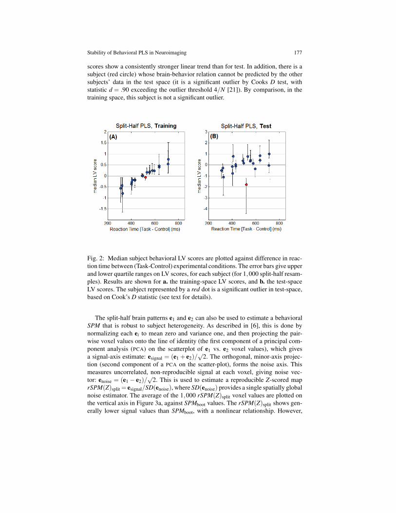
Stability of Behavioral PLS in Neuroimaging 177

scores show a consistently stronger linear trend than for test. In addition, there is asubject (red circle) whose brain-behavior relation cannot be predicted by the othersubjects’ data in the test space (it is a significant outlier by Cooks D test, withstatistic d = .90 exceeding the outlier threshold 4/N [21]). By comparison, in thetraining space, this subject is not a significant outlier.

Fig. 2: Median subject behavioral LV scores are plotted against difference in reac-tion time between (Task-Control) experimental conditions. The error bars give upperand lower quartile ranges on LV scores, for each subject (for 1,000 split-half resam-ples). Results are shown for a. the training-space LV scores, and b. the test-spaceLV scores. The subject represented by a red dot is a significant outlier in test-space,based on Cook’s D statistic (see text for details).

The split-half brain patterns e1 and e2 can also be used to estimate a behavioralSPM that is robust to subject heterogeneity. As described in [6], this is done bynormalizing each ei to mean zero and variance one, and then projecting the pair-wise voxel values onto the line of identity (the first component of a principal com-ponent analysis (PCA) on the scatterplot of e1 vs. e2 voxel values), which givesa signal-axis estimate: esignal = (e1 + e2)/

02. The orthogonal, minor-axis projec-

tion (second component of a PCA on the scatter-plot), forms the noise axis. Thismeasures uncorrelated, non-reproducible signal at each voxel, giving noise vec-tor: enoise = (e1$ e2)/

02. This is used to estimate a reproducible Z-scored map

rSPM(Z)split = esignal/SD(enoise), where SD(enoise) provides a single spatially globalnoise estimator. The average of the 1,000 rSPM(Z)split voxel values are plotted onthe vertical axis in Figure 3a, against SPMboot values. The rSPM(Z)split shows gen-erally lower signal values than SPMboot, with a nonlinear relationship. However,

178 Churchill et al.

this difference is partly a function of the global versus local noise estimators. Wecan instead estimate the mean esignal value at each voxel, and normalize by the SDon enoise for each voxel (each computed across 1,000 resamples), generating voxel-wise estimates of noise in the same manner as SPMboot. This rSPM(Z) is plottedagainst SPMboot in Figure 3b, demonstrating a strong linear trend, albeit with in-creased scatter for high-signal voxels. This scatter is primarily due to differences inthe local noise estimates: the mean bootstrap LV and esignal patterns are highly con-sistent (correlation equal to .99), whereas the local noise estimates are more variablebetween the two methods (plotted in Figure 3c; correlation equal to .86).

Fig. 3: Scatter plot of pairs of voxel SPM values: we compare standard bootstrappedbehavioral PLS analysis producing (mean voxel salience)/(standard error), to split-half signal/noise estimates. This includes a. standard NPAIRS estimation of voxelsignal, normalized by global noise standard deviation (Z-scored) for each resample,and b. voxel signal, normalized by standard error (bootstrap ratios) or standard de-viation (split-half Z-scores) estimated at each voxel. c. plot of voxels’ standard error(bootstrap) against standard deviation (split-half). Results are computed over 1,000split-half/bootstrap resamples.

2.3 Behavioral PLS on a principal component subspace

For standard behavioral PLS, we project the behavioral vector y directly onto X(the subject SPMs) to identify the latent basis vector e = yTX. However, taking ourcue from the literature on split-half discriminant analysis in f MRI (see, e.g., [7, 10,18, 19, 22]), we can regularize and de-noise the data space in which the analysis isperformed, by first applying PCA to X, and then running a PLS analysis on a reducedPCA subspace.

The singular value decomposition [20] produces X = USVT, where U is a setof orthonormal subject-weight vectors, S is a diagonal matrix of singular values,and V is a set of orthonormal image basis vectors. We represent X in a reduced k-

Stability of Behavioral PLS in Neuroimaging 179

dimensional PCA space (k(N), by projecting onto the subset of 1 to k image bases,V(k) = [v1v2 . . .vk], giving Q(k) = XV(k). We performed PLS analysis on Q(k), bynormalizing and centering subject scores of each PC-basis, and then obtaining theprojection wi = yTi Qi that explained the most behavior variance in the new PC basis.

Fig. 4: a. Plot of median predicted behavioral correlation rtest and spatial repro-ducibility rspatial of the LV brain map, for PLS performed on a PCA subspace of thesubject data (blue). These subspaces include the 1 to k Principal Components (PCs),where we vary (1 ( k ( 10). The (rspatial, rtest) values are plotted for each k (sub-space size) as points on the curve; a subspace of PCs 1–4 simultaneously optimized(rspatial, rtest), circled in black. We also plot the median (rtest,rspatial) point, estimateddirectly from matrix X for reference (red circle). b. Plots of split-half Z-scored SPMswith global noise estimation, for no PCA estimation (red), and an optimized PCA di-mensionality k = 4 (blue). Positive Z-scores indicate positive correlation with thebehavioral measure of reaction time, and negative Z-scores indicate negative corre-lation. Voxel values are computed as the mean over 1,000 split-half resamples, withspatially global noise estimation from each split-half pair.

The predicted behavioral correlation is measured by projecting the test data ontothe training PC-space, and then onto wi, giving behavioral correlations r(i,test) =7(y j )=i,wi(X j )=iVi). We also obtained eigen-images by projecting back onto thevoxel space (i.e., ei = wiV(k)

i ), to compute the rSPM(Z)split and reproducibility,rspatial. The resulting median behavioral prediction r(test) and reproducibility r(spatial)are plotted in Figure 4a, as a function of the number of PC bases k. From this curve,we identify the PC subspace k = 4, that maximizes both rtest and rspatial. Note thatthe median rtest and rspatial are consistently higher when performed on a PCA basis

180 Churchill et al.

than PLS performed directly on X, for all subspace sizes k = 1 . . .10. The predictedbehavioral correlation is generally higher for the k = 4 PC subspace than PLS per-formed directly on X (median 1rtest = .17; increased for 891 of the 1,000 resam-ples), as is spatial reproducibility (1rspatial = .05; increased for all 1,000 resam-ples). Figure 4b depicts slices from the mean rSPM(Z)s of PLS performed directlyon X (top) and in an optimized PC subspace (bottom). The PCA optimization tendsto increase mean Z-scores in the same areas of activation previously identified byvoxel-space results, indicating that the optimized PC basis increases sensitivity ofthe PLS model to the same underlying set of brain regions.

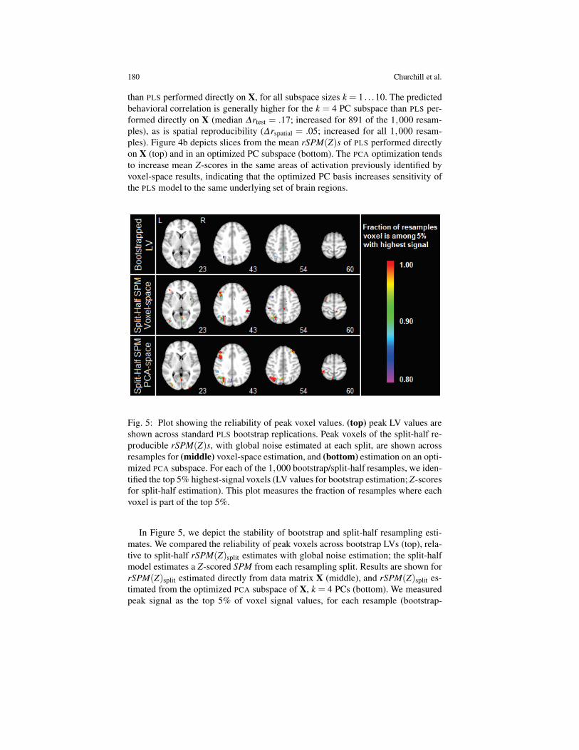
Fig. 5: Plot showing the reliability of peak voxel values. (top) peak LV values areshown across standard PLS bootstrap replications. Peak voxels of the split-half re-producible rSPM(Z)s, with global noise estimated at each split, are shown acrossresamples for (middle) voxel-space estimation, and (bottom) estimation on an opti-mized PCA subspace. For each of the 1,000 bootstrap/split-half resamples, we iden-tified the top 5% highest-signal voxels (LV values for bootstrap estimation; Z-scoresfor split-half estimation). This plot measures the fraction of resamples where eachvoxel is part of the top 5%.

In Figure 5, we depict the stability of bootstrap and split-half resampling esti-mates. We compared the reliability of peak voxels across bootstrap LVs (top), rela-tive to split-half rSPM(Z)split estimates with global noise estimation; the split-halfmodel estimates a Z-scored SPM from each resampling split. Results are shown forrSPM(Z)split estimated directly from data matrix X (middle), and rSPM(Z)split es-timated from the optimized PCA subspace of X, k = 4 PCs (bottom). We measuredpeak signal as the top 5% of voxel signal values, for each resample (bootstrap-

Stability of Behavioral PLS in Neuroimaging 181

estimated LV scores or split-half-estimated Z-scores). At each voxel, we measuredthe fraction of resamples where it was a peak voxel (i.e., among the top 5%). Forbootstrap LVs, only 2 of 37,284 voxels (less than .001%) were active in morethan 95% of resamples, compared to split-half Z-scored estimates of 324 voxels(0.87%; PLS computed on X) and 343 voxels (0.92%; PLS on an optimized PCAbasis). This demonstrates that although rSPM(Z)split with global noise estimationproduces lower mean signal values than SPMboot (Figure 3a), the location of peakrSPM(Z)split values are highly stable across resampling splits. We can thereforeidentify reliable SPM peaks with relatively few resampling iterations.

2.4 Behavioral PLS and optimized preprocessing

For results in Sections 2.2 and 2.3, we preprocessed the f MRI data to correct fornoise and artifact, as outlined in [18, 19]. For this procedure, we included/excludedevery combination of the preprocessing steps: (1) motion correction, (2) physiolog-ical correction, (3) regressing head-motion covariates and (4) temporal detrendingwith Legendre polynomial of orders 0 to 5, evaluating 23" 6 = 48 different combi-nations of preprocessing steps (“pipelines”).

For each pipeline, we performed an analysis in the NPAIRS split-half frame-work [6], and measured spatial reproducibility and prediction accuracy (posteriorprobability of correctly classifying independent scan volumes). We selected thepipeline that minimized the Euclidean distance from perfect prediction and repro-ducibility:

D =8(1$ reproducibility)2 +(1$ prediction)2, (2)

independently for each subject. This may be compared to the standard approach inf MRI literature, which is to apply a single fixed pipeline to all subjects. We comparedthe current “individually optimized” results with the optimal “fixed pipeline,” ofmotion correction and 3rd-order detrending; this was the set of steps that, applied toall subjects, minimized the D metric across subjects (details in [18]).

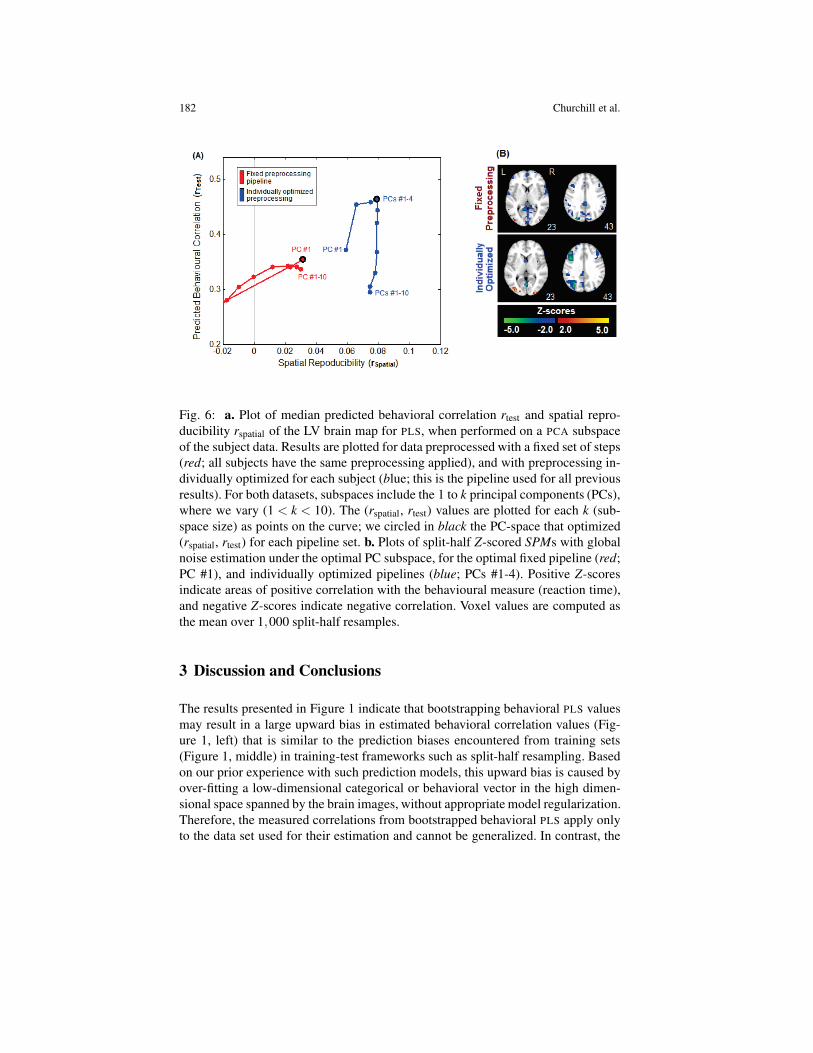
Figure 4 compares fixed pipeline results (red) to individually optimized data(blue), for PLS on a PCA subspace. Figure 4a show, for both pipelines, median be-havioral prediction r(test) and reproducibility r(spatial) plotted as a function of PCAdimensionality. Data with fixed preprocessing (red) optimized r(test) and r(spatial) atPC #1, a lower dimensionality than individually optimized preprocessing (blue), atPCs #1–4. For the optimized PC bases (circled in black), individual pipeline opti-mization improves over fixed pipelines with median 1r(test) = .11 (increased for 898out of the 1,000 resamples), and 1r(spatial) = .06 (increased for 810 out of the 1,000resamples). Figure 4b shows sample slices from the mean Z-scored SPMs, in the op-timized PC subspaces. Individual subject pipeline optimization generally produceshigher peak Z-scores, and sparser, less noisy SPMs, than fixed preprocessing.

182 Churchill et al.

Fig. 6: a. Plot of median predicted behavioral correlation rtest and spatial repro-ducibility rspatial of the LV brain map for PLS, when performed on a PCA subspaceof the subject data. Results are plotted for data preprocessed with a fixed set of steps(red; all subjects have the same preprocessing applied), and with preprocessing in-dividually optimized for each subject (blue; this is the pipeline used for all previousresults). For both datasets, subspaces include the 1 to k principal components (PCs),where we vary (1 < k < 10). The (rspatial, rtest) values are plotted for each k (sub-space size) as points on the curve; we circled in black the PC-space that optimized(rspatial, rtest) for each pipeline set. b. Plots of split-half Z-scored SPMs with globalnoise estimation under the optimal PC subspace, for the optimal fixed pipeline (red;PC #1), and individually optimized pipelines (blue; PCs #1-4). Positive Z-scoresindicate areas of positive correlation with the behavioural measure (reaction time),and negative Z-scores indicate negative correlation. Voxel values are computed asthe mean over 1,000 split-half resamples.

3 Discussion and Conclusions

The results presented in Figure 1 indicate that bootstrapping behavioral PLS valuesmay result in a large upward bias in estimated behavioral correlation values (Fig-ure 1, left) that is similar to the prediction biases encountered from training sets(Figure 1, middle) in training-test frameworks such as split-half resampling. Basedon our prior experience with such prediction models, this upward bias is caused byover-fitting a low-dimensional categorical or behavioral vector in the high dimen-sional space spanned by the brain images, without appropriate model regularization.Therefore, the measured correlations from bootstrapped behavioral PLS apply onlyto the data set used for their estimation and cannot be generalized. In contrast, the

Stability of Behavioral PLS in Neuroimaging 183

much lower split-half test estimates of behavioral correlation in Figure 1 (right) aregeneralizable but are potentially biased downwards, being based on relatively smalltraining/test groups of only 10 subjects.

Non-generalizable training bias is also reflected in the plots of median LV scoresvs. behavioral measures, in Figure 2. If the scores are computed from the training-space estimates, we obtain a stronger linear trend and less variability across splits,compared to independent test data projected onto the training basis. As shown inFigure 2, plotting the test-space scores may also reveal potential prediction outliersthat are not evident in the training plots.

The Figure 3a plot also shows that bootstrapped peak SPM signals are consis-tently higher than standard split-half global Z-scoring. However, Figure 3b showsthat on this is primarily a function of the different noise estimators, as the voxel-wise, split-half noise estimation SPM is highly correlated with the bootstrap esti-mated SPM. Both of the scatter-plots show a strong monotonic relation betweenSPMboot and the rSPM(Z)s, indicating that regardless of the estimation procedure,approximately the same spatial locations drive both bootstrap and split-half anal-yses. Even for voxel-wise noise estimation, the difference between split-half andbootstrap SPMs is primarily driven by the local noise estimates (plotted in Fig-ure 3c), whereas mean signal values are highly similar.

Figure 4 shows that the original X data space can be better regularized and sta-bilized, by projecting data onto a PC subspace prior to analysis. By adapting thenumber of PC dimensions, we trace out a behavioral correlation vs. reproducibilitycurve as a function of the number of PCs, similar to the prediction vs. reproducibil-ity curves observed in discriminant models [10, 22]. These results highlight, again,the ill-posed nature of the PLS data-analysis problem, and the importance of reg-ularizing f MRI data. We also note that even a full-dimensionality PC-space model(e.g., PCs 1-10 included in each split-half) outperforms estimation directly on thematrix X. The PCA projects data onto the bases of maximum variance, prior to stan-dard PLS normalization (giving zero mean and unit variance to scores of each PCbasis). The superior performance of PCs 1-10 over no PC basis (Figure 4) indicatesthat the variance normalization in voxel space may significantly limit the predictivegeneralizability of behavioral PLS results for some analyses.

Figure 5 demonstrates the advantages of split-half resampling with global noiseestimation. For each split, we generate a single Z-scored rSPM(Z), for which peakvoxels tend to be highly consistent across rSPM(Z)s of individual resampling splits.This allows us to measure voxel Z-scores on a little as one resampling split. Thestability of the peak activations also allows us to identify reliable brain regions froma single split, which is not available to voxel-wise bootstrap estimation. The cross-validation framework is therefore particularly useful when only limited f MRI data isavailable, and has been previously used to optimize preprocessing in brief task runsof less than 3 minutes in length (e.g., [18, 19]).

The results of Figure 4 compared data with preprocessing choices optimized onan individual subject basis, relative to the standard f MRI approach of using a singlefixed pipeline. Results indicate that optimizing preprocessing choices on an individ-ual subject basis can significantly improve predicted test correlation and the spatial

184 Churchill et al.

reproducibility of LV maps in behavioral PLS. Note that pipeline optimization wasperformed independently of any behavioral measures, as we chose preprocessingsteps to optimize SPM reproducibility and prediction accuracy of the linear dis-criminant analysis model. These results demonstrate that improved preprocessingmay help to better detect brain-behavior relationships in f MRI data.

References

1. D. Wilkinson, and P. Halligan, “The relevance of behavioral measures for functional-imagingstudies of cognition,” Nature Review Neuroscience 5, pp. 67–73, 2004.

2. A. R. McIntosh, “Mapping cognition to the brain through neural interactions,” Memory 7,pp. 523–548, 1999.

3. A. Krishnan, L. J. Williams, A. R. McIntosh, and H. Abdi, “Partial Least Squares (PLS) meth-ods for neuroimaging: A tutorial and review,” Neuroimage 56, pp. 455–475, 2011.

4. N. Morch, L. K. Hansen, S. C. Strother, C. Svarer, D. .A. Rottenberg, B. Lautrup, R. Savoy,and O. B. Paulson, “Nonlinear versus linear models in functional neuroimaging: Learningcurves and generalization crossover,” Information Processing in Medical Imaging, J. Duncanand G. Gindi, eds.; Springer-Verlag, New York, pp. 259–270, 1997.

5. A. J. O’Toole, F. Jiang, H. Abdi, N. Penard, J. P. Dunlop, and M. A. Parent, “Theoretical, sta-tistical, and practical perspectives on pattern-based classification approaches to the analysis offunctional neuroimaging data,” Journal of Cognitive Neuroscience 19, pp. 1735–1752, 2007.

6. S. C. Strother, J. Anderson, L. K. Hansen, U. Kjems, R. Kustra, J. Sidtis, S. Frutiger, S. Mu-ley, S. LaConte, and D. Rottenberg, “The quantitative evaluation of functional neuroimagingexperiments: the NPAIRS data analysis framework,” Neuroimage 15, pp. 747–771, 2002.

7. S. C. Strother, S. LaConte, L. K. Hansen, J. Anderson, J. Zhang, S. Pulapura, and D. Rot-tenberg, “Optimizing the f MRI data-processing pipeline using prediction and reproducibilityperformance metrics: I. A preliminary group analysis,” Neuroimage 23 Suppl 1, pp. S196–S207, 2004.

8. S. C. Strother, “Evaluating f MRI preprocessing pipelines,” IEEE Engineering in Medicineand Biology Magazine 25, pp. 27–41, 2006

9. H. Abdi, J. P. Dunlop, and L. J. Williams, “How to compute reliability estimates and dis-play confidence and tolerance intervals for pattern classifiers using the Bootstrap and 3-waymultidimensional scaling (DISTATIS),” Neuroimage 45, pp. 89–95, 2009.

10. S. Strother, A. Oder, R. Spring, and C. Grady, “The NPAIRS Computational statistics frame-work for data analysis in neuroimaging,” presented at the 19th International Conference onComputational Statistics, Paris, France, 2010.

11. R. Kustra, and S. C. Strother, “Penalized discriminant analysis of [15O]-water PET brainimages with prediction error selection of smoothness and regularization hyperparameters,”IEEE Transactions in Medical Imaging 20, pp. 376–387, 2001.

12. N. Meinshausen, and P. Buhlmann, “Stability selection,” Journal of the Royal Statistical So-ciety: Series B (Statistical Methodology) 72, pp. 417–473, 2010.

13. K. V. Mardia, J. T. Kent, and J. M. Bibby, Multivariate Analysis, Academic Press, London,1979.

14. H. Abdi, “Partial least squares regression and projection on latent structure regression (PLSRegression),” WIREs Computational Statistics 2, pp. 97–106, 2010.

15. J. G. Snodgrass, and M. Vanderwart, “A standardized set of 260 pictures: norms for nameagreement, image agreement, familiarity, and visual complexity,” Journal of ExperimentalPsychology: Human Learning 6, pp. 174–215, 1980.

16. C. Grady, M. Springer, D. Hongwanishkul, A. R. McIntosh, and G. Winocur, “Age-relatedchanges in brain activity across the adult fifespan: A failure of inhibition?,” Journal of Cogni-tive Neuroscience 18, pp. 227–241, 2006.

Stability of Behavioral PLS in Neuroimaging 185

17. F. Tam, N. W. Churchill, S. C. Strother, and S. J. Graham, “A new tablet for writing anddrawing during functional MRI,” Human Brain Mapping 32, pp. 240–248, 2011.

18. N. W. Churchill, A. Oder, H. Abdi, F. Tam, W. Lee, C. Thomas, J. E. Ween, S. J. Graham, andS. C. Strother, “Optimizing preprocessing and analysis pipelines for single-subject f MRI: I.Standard temporal motion and physiological noise correction methods,” Human Brain Map-ping 33, pp. 609–627, 2012.

19. N. W. Churchill, G. Yourganov, A. Oder, F. Tam, S. J. Graham, and S. C. Strother, “Optimizingpreprocessing and analysis pipelines for single-subject f MRI: 2. Interactions with ICA, PCA,task contrast and inter-subject heterogeneity,” PLoS One 7, (e31147), 2012.

20. H. Abdi, “Singular value decomposition (SVD) and generalized singular value decomposition(GSVD),” in Encyclopedia of Measurement and Statistics, N. Salkind, ed., pp. 907–912, Sage,Thousand Oaks, 2007.

21. K. A. Bollen, and R. W. Jackman, “Regression diagnostics: An expository treatment of outliersand influential cases,” in J. Fox, and J.S. Long, (eds.), Modern Methods of Data Analysis, pp.257–291. Sage, Newbury Park, 2012.

22. P. M. Rasmussen, L. K. Hansen, K. H. Madsen, N. W. Churchill, and S. C. Strother, “Patternreproducibility, interpretability, and sparsity in classification models in neuroimaging,” PatternRecognition 45, pp. 2085–2100, 2012.