Embed Size (px)
Citation preview
THE SPECTRAL MODELING TOOLBOX: A SOUND
ANALYSIS/SYNTHESIS SYSTEM
A Thesis
Submitted to the Faculty
in partial fulfillment of the requirements for the
degree of
Master of Arts
in
ELECTRO-ACOUSTIC MUSIC
by
Micah Kimo Johnson
DARTMOUTH COLLEGE
Hanover, New Hampshire
May 29, 2002
Examining Committee:
(Chair) Larry Polansky
Eric Lyon
Metin Akay
Carol FoltDean of Graduate Studies

c© 2002 Micah Kimo Johnson
All Rights Reserved
i
Abstract
This thesis describes the Spectral Modeling Toolbox, a collection of functions
for digitally analyzing and synthesizing sound. The techniques in the Toolbox
generalize the concepts of other analysis/synthesis systems in an environment
created for algorithm design and research. The design decisions and basic tech-
niques are documented in this thesis, and complete source code for the Tool-
box is available. The Spectral Modeling Toolbox is an introduction to analy-
sis/synthesis techniques, a spectral processing tool, and perhaps, the foundation
for future sound recognition systems.
ii
Acknowledgments
I would like to thank Larry Polanksy, Jon Appleton, Eric Lyon, and Charles
Dodge for changing the way I think about music and for providing the supportive
environment in which I produced this work.
I would also like to thank Metin Akay for pushing my research along and for
believing that I could solve problems even when I could not see the solution.
Finally, I would like to thank my parents for encouraging me and never
trying to limit my aspirations.
This thesis is dedicated to Amity, whose love and patience inspire me.
iii
Contents
Abstract ii
Acknowledgments iii
Table of Contents iv
List of Tables vii
List of Figures viii
1 Introduction 1
1.1 Representations of Sound for Artificial Recognition . . . . . . . 2
1.2 An Overview of the Spectral Modeling Toolbox . . . . . . . . . 3
1.3 Thesis Structure . . . . . . . . . . . . . . . . . . . . . . . . . . . 4
2 Signals in Time and Frequency 6
2.1 A Basis for a Space . . . . . . . . . . . . . . . . . . . . . . . . . 7
2.2 Short-Time Fourier Transform . . . . . . . . . . . . . . . . . . . 9
2.3 Wavelet Transform . . . . . . . . . . . . . . . . . . . . . . . . . 13
2.4 A Comparison of Two Time-Frequency Transforms . . . . . . . 15
2.4.1 The Signals . . . . . . . . . . . . . . . . . . . . . . . . . 16
2.4.2 Analysis Techniques . . . . . . . . . . . . . . . . . . . . 17
2.4.3 Results . . . . . . . . . . . . . . . . . . . . . . . . . . . . 19
2.4.4 Conclusions . . . . . . . . . . . . . . . . . . . . . . . . . 26
3 Analysis/Synthesis Systems 28
3.1 The Phase Vocoder . . . . . . . . . . . . . . . . . . . . . . . . . 29
3.2 The McAulay-Quatieri Analysis/Synthesis Technique . . . . . . 30
3.3 Spectral Modeling Synthesis . . . . . . . . . . . . . . . . . . . . 32
3.4 Design of the Spectral Modeling Toolbox . . . . . . . . . . . . . 34
iv
3.4.1 TF Analysis . . . . . . . . . . . . . . . . . . . . . . . . . 34
3.4.2 Detect Peaks . . . . . . . . . . . . . . . . . . . . . . . . 35
3.4.3 Psychoacoustic Model . . . . . . . . . . . . . . . . . . . 36
3.4.4 TF Tracks . . . . . . . . . . . . . . . . . . . . . . . . . . 37
3.4.5 Residual . . . . . . . . . . . . . . . . . . . . . . . . . . . 38
3.4.6 Data Modification . . . . . . . . . . . . . . . . . . . . . 38
3.4.7 Place Peaks . . . . . . . . . . . . . . . . . . . . . . . . . 39
3.4.8 TF Synthesis . . . . . . . . . . . . . . . . . . . . . . . . 39
4 The Spectral Modeling Toolbox 40
4.1 Installing the Toolbox . . . . . . . . . . . . . . . . . . . . . . . 40
4.2 Reading and Writing Audio Files . . . . . . . . . . . . . . . . . 40
4.3 TF Analysis and TF Synthesis . . . . . . . . . . . . . . . . . . . 41
4.4 Detect Peaks and Place Peaks . . . . . . . . . . . . . . . . . . . 44
4.5 Psychoacoustic Model . . . . . . . . . . . . . . . . . . . . . . . 46
4.6 TF Tracks . . . . . . . . . . . . . . . . . . . . . . . . . . . . . . 47
4.7 Modification Functions . . . . . . . . . . . . . . . . . . . . . . . 49
4.8 Using Wavelets for Analysis and Synthesis . . . . . . . . . . . . 49
5 Conclusions and Future Directions 51
List of References 53
A Basic Signal Processing in MATLAB 55
A.1 Sampling . . . . . . . . . . . . . . . . . . . . . . . . . . . . . . . 55
A.2 The Complex Exponential . . . . . . . . . . . . . . . . . . . . . 59
A.3 Discrete Fourier Transform . . . . . . . . . . . . . . . . . . . . . 62
A.4 Windows . . . . . . . . . . . . . . . . . . . . . . . . . . . . . . . 70
v
B Beyond the Basics 73
B.1 Parabolic Interpolation . . . . . . . . . . . . . . . . . . . . . . . 73
B.2 Zero-Padding . . . . . . . . . . . . . . . . . . . . . . . . . . . . 76
B.3 Centering the FFT Buffer for Phase Estimation . . . . . . . . . 78
C Important Mathematical Proofs and Derivations 84
C.1 The Euler Formula . . . . . . . . . . . . . . . . . . . . . . . . . 84
C.2 Parabolic Interpolation . . . . . . . . . . . . . . . . . . . . . . . 84
C.3 Shift Property of the Fourier Transform . . . . . . . . . . . . . . 86
Bibliography 87
vi
List of Tables
2.1 Frequency error and width . . . . . . . . . . . . . . . . . . . . . 23
2.2 Start time and duration . . . . . . . . . . . . . . . . . . . . . . 24
vii
List of Figures
1.1 The Spectral Modeling Toolbox . . . . . . . . . . . . . . . . . . 3
2.1 A signal multiplied by a window function . . . . . . . . . . . . . 10
2.2 A Hamming window . . . . . . . . . . . . . . . . . . . . . . . . 12
2.3 Shifted and scaled wavelets . . . . . . . . . . . . . . . . . . . . . 14
2.4 The Morlet wavelet . . . . . . . . . . . . . . . . . . . . . . . . . 16
2.5 Music notation for the test signals . . . . . . . . . . . . . . . . . 17
2.6 Center frequency, frequency width, start time, and duration . . 18
2.7 Analysis of the arpeggio . . . . . . . . . . . . . . . . . . . . . . 20
2.8 Analysis of the scale . . . . . . . . . . . . . . . . . . . . . . . . 21
2.9 Analysis of the chord progression . . . . . . . . . . . . . . . . . 22
2.10 Center frequency error and frequency width. . . . . . . . . . . . 25
2.11 Start time and duration error. . . . . . . . . . . . . . . . . . . . 25
3.1 The phase vocoder . . . . . . . . . . . . . . . . . . . . . . . . . 29
3.2 Forming sinusoid tracks . . . . . . . . . . . . . . . . . . . . . . 31
3.3 The MQ analysis/synthesis system . . . . . . . . . . . . . . . . 32
3.4 Spectral Modeling Synthesis . . . . . . . . . . . . . . . . . . . . 34
3.5 The Spectral Modeling Toolbox . . . . . . . . . . . . . . . . . . 35
3.6 The minimum audible field curve . . . . . . . . . . . . . . . . . 36
3.7 Masking curves . . . . . . . . . . . . . . . . . . . . . . . . . . . 37
4.1 The STFT of a saxophone note . . . . . . . . . . . . . . . . . . 42
4.2 A frame of the STFT . . . . . . . . . . . . . . . . . . . . . . . . 44
4.3 The output of smt detectPeaks . . . . . . . . . . . . . . . . . . 45
4.4 The psychoacoustic model reduces the number of peaks . . . . . 46
4.5 The amplitude and frequency trajectory of a harmonic . . . . . 47
4.6 Filtering peaks with smt filterPeaks . . . . . . . . . . . . . . . . 48
viii
4.7 The CWT of the saxophone note . . . . . . . . . . . . . . . . . 50
A.1 A sampled cosine wave . . . . . . . . . . . . . . . . . . . . . . . 56
A.2 Sampling a signal below the Nyquist frequency . . . . . . . . . . 57
A.3 Sampling signals above the Nyquist frequency . . . . . . . . . . 59
A.4 Motion around a circle . . . . . . . . . . . . . . . . . . . . . . . 60
A.5 Sampling the frequency domain . . . . . . . . . . . . . . . . . . 63
A.6 The DFT of real signals . . . . . . . . . . . . . . . . . . . . . . 69
A.7 The DFT of a 2.2 Hz sine wave . . . . . . . . . . . . . . . . . . 70
A.8 A windowed sine wave . . . . . . . . . . . . . . . . . . . . . . . 71
B.1 The main peak of a magnitude spectrum . . . . . . . . . . . . . 74
B.2 A zero-padded signal . . . . . . . . . . . . . . . . . . . . . . . . 76
B.3 The spectrum of a zero-padded signal . . . . . . . . . . . . . . . 77
B.4 The phase spectrum of a sinusoid . . . . . . . . . . . . . . . . . 78
B.5 Shifting a signal for phase estimation . . . . . . . . . . . . . . . 79
B.6 The phase spectrum after shifting . . . . . . . . . . . . . . . . . 80
B.7 A cosine with a phase offset of π/4 . . . . . . . . . . . . . . . . 82
ix
1 Introduction
Sound begins with a vibration. The vibration pushes and pulls on the surround-
ing air molecules, creating small variations in air pressure that travel away from
the vibration as a sound wave. If we are in the path of the sound wave, the
pressure variations move down our ear canal to our eardrum. The auditory
system converts the vibration of the eardrum into nerve firings, which our brain
arranges into auditory sensations. By deciphering the air pressure patterns we
learn that a car passed by outside or that a neighbor is mowing his lawn.
Most people do not consider the complexity of sound perception because of
the ease with which it occurs. We are surrounded by sounds all day long and it
usually requires little effort to separate them into objects or events [1, p. 180].
Sound recognition also occurs with ease; we rarely confuse a cat’s meow for a
dog’s bark. The ability to separate and recognize sound sources is important to
our perception of music. It allows us to separate the sound of a soloist from the
sound of the accompaniment and to distinguish a string quartet from a brass
quartet.
How did we learn to separate and recognize sounds? Gestalt psychologists
believe that we are born with an understanding of the basic laws of perceptual
organization [2, p. 39–40]. These laws influence the learning process by enabling
us to parse our auditory environment. From birth, we learn to organize sounds
and the ease with which perception occurs later in life is the result of years of
work.
The auditory system can also be trained to recognize small details in a sound.
For example, some musicians can distinguish between the sound of a coronet
and the sound of a trumpet. Music students who have taken several semesters
of ear training can identify many different chords and intervals; some can even
1
transcribe four-voice chorals. In the last example, there is a conscious effort to
train the auditory system to recognize sounds. It is a difficult task for many,
but it is possible with enough practice.
While training our auditory system to recognize sounds may be difficult,
training a computer to recognize sounds is even more complex. This is true for
many tasks that fall under the category of artificial intelligence; it is difficult to
program current computers to imitate human thought. Of course, computers
can perform tasks that are nearly impossible for humans: try finding the next
prime number after 213,466,917 − 1. Someday, I believe computer systems will be
able to recognize and separate sound sources. One approach towards this goal
is to use knowledge of the auditory system in the design of these systems.
1.1 Representations of Sound for Artificial Recognition
This thesis describes a sound analysis and synthesis system that incorporates
knowledge of the auditory system. Analysis/synthesis systems are powerful
sound processing tools: they can decompose sounds into simple components
and synthesize sounds from these components.
Analysis/synthesis systems are often used for psychoacoustic research and
music composition. They have been used in studies on instrument timbre to
reduce sounds to basic elements and then to synthesize sounds from these el-
ements. A human can then compare the synthesized sound to the original to
determine if the basic elements completely describe the sound. In music compo-
sition, they allow for various sound processing and transformation techniques.
Time scaling, pitch shifting, cross synthesis, and spectral morphing are all pos-
sible with these systems. Analysis/synthesis systems could also be the first step
towards artificial recognition of sound sources since most of the information
extracted by such systems is important to perception.
2
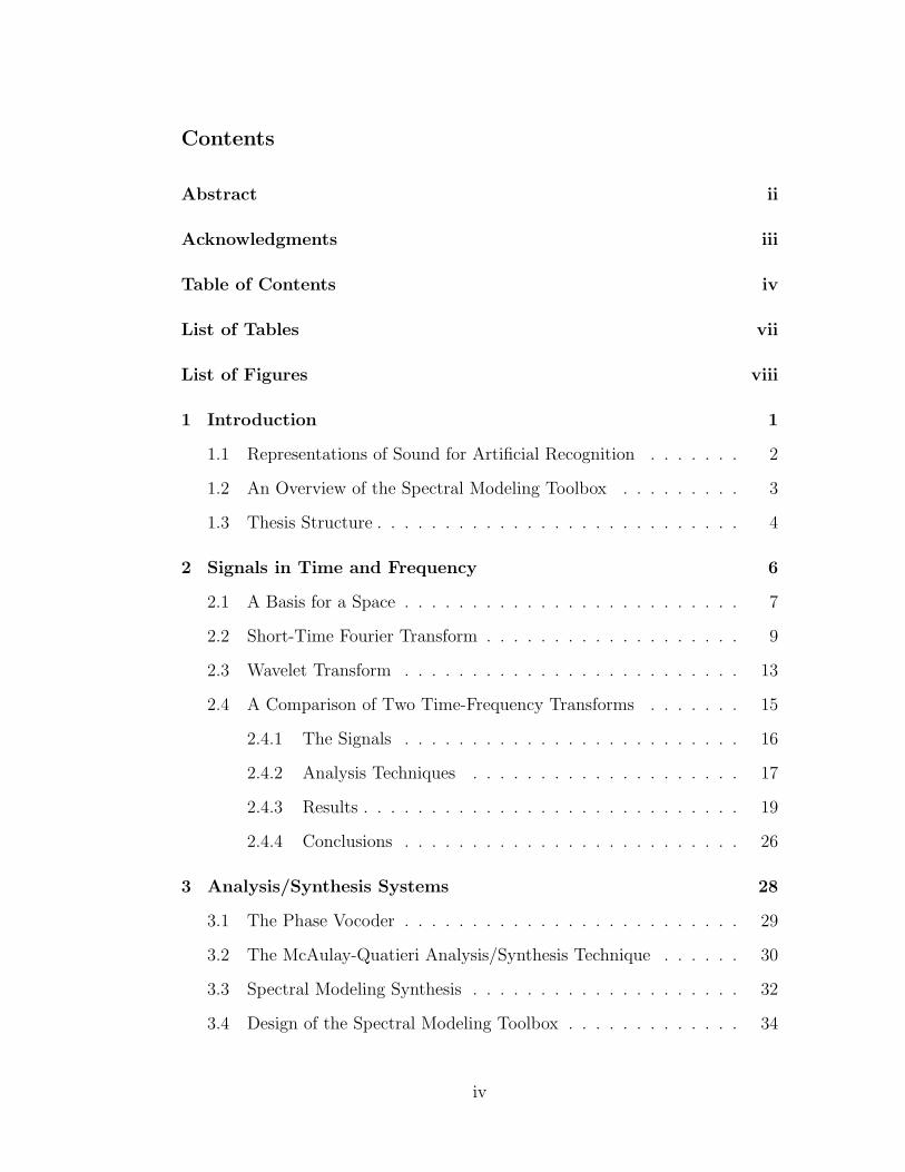
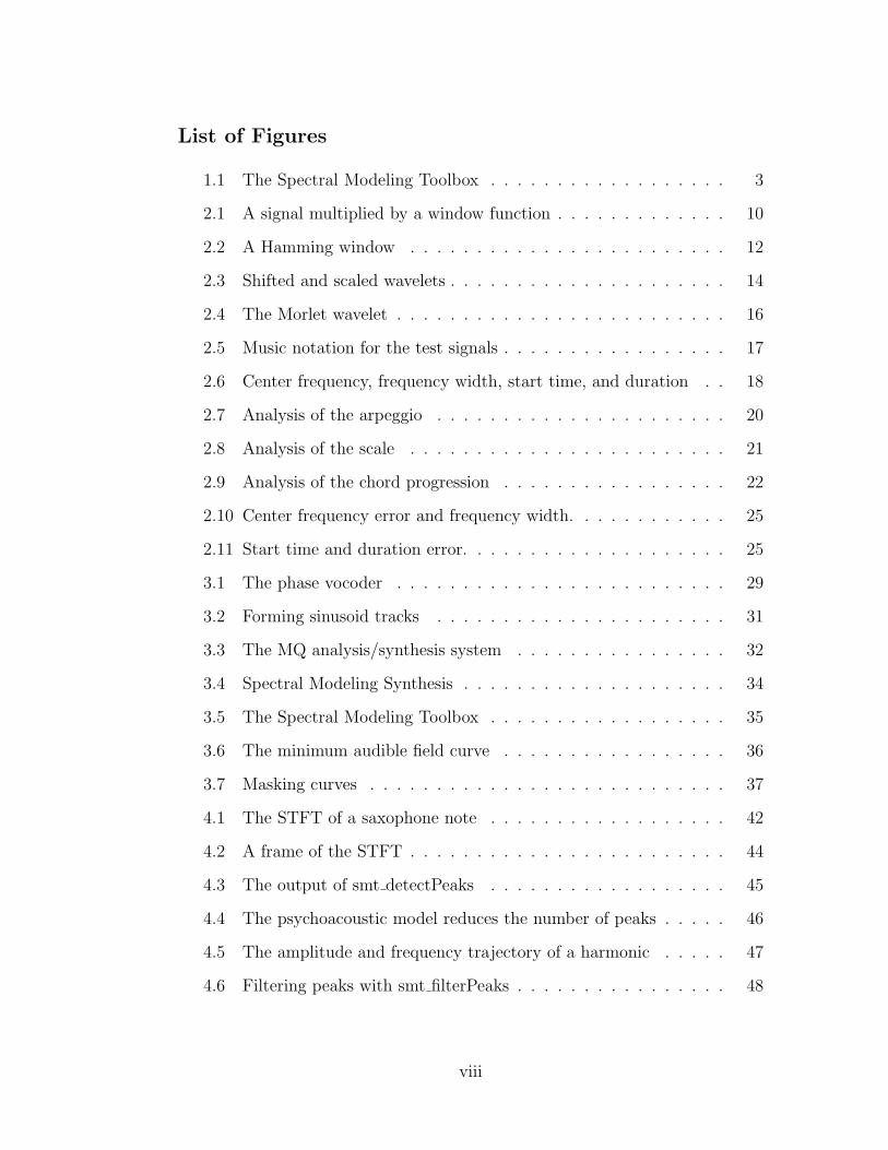
TF Analysis Detect Peaks Place Peaks TF SynthesisSound File Sound File
PsychoacousticModel
TF Tracks
Analysis Synthesis
Residual
DataModification
DataModification
FilteredNoise
Opt
iona
l Pro
cess
ing
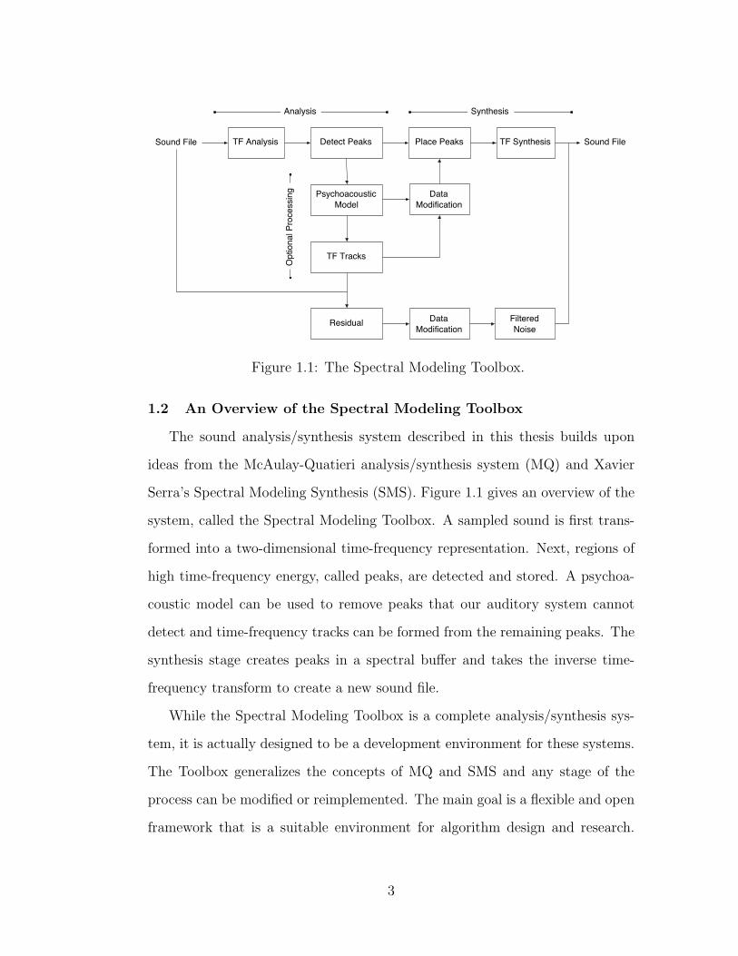
Figure 1.1: The Spectral Modeling Toolbox.
1.2 An Overview of the Spectral Modeling Toolbox
The sound analysis/synthesis system described in this thesis builds upon
ideas from the McAulay-Quatieri analysis/synthesis system (MQ) and Xavier
Serra’s Spectral Modeling Synthesis (SMS). Figure 1.1 gives an overview of the
system, called the Spectral Modeling Toolbox. A sampled sound is first trans-
formed into a two-dimensional time-frequency representation. Next, regions of
high time-frequency energy, called peaks, are detected and stored. A psychoa-
coustic model can be used to remove peaks that our auditory system cannot
detect and time-frequency tracks can be formed from the remaining peaks. The
synthesis stage creates peaks in a spectral buffer and takes the inverse time-
frequency transform to create a new sound file.
While the Spectral Modeling Toolbox is a complete analysis/synthesis sys-
tem, it is actually designed to be a development environment for these systems.
The Toolbox generalizes the concepts of MQ and SMS and any stage of the
process can be modified or reimplemented. The main goal is a flexible and open
framework that is a suitable environment for algorithm design and research.
3
The Toolbox is distributed as a collection of MATLAB functions complete with
source code and documentation.
I chose to implement the Toolbox in MATLAB because of the high degree
of functionality already available in it. MATLAB is a commercial product
designed for mathematical computation, analysis, visualization, and algorithm
development. It has many functions that handle everything from simple plotting
to statistical analysis and signal processing. There are also toolboxes available
that extend its features to include wavelets, neural networks, curve fitting, and
other specialized tasks.
The major disadvantage of the MATLAB platform is efficiency; the same
algorithms written in C++ would be much faster. Since the Toolbox is meant
to be an environment for research, efficiency is sacrificed to gain functionality.
The tools available in MATLAB facilitate algorithm development and once these
algorithms function properly, they can be coded in another language to improve
efficiency.
While the primary goal was to create a flexible analysis/synthesis environ-
ment, this thesis can also serve as a reference for designers of sound processing
systems. All of the details—from design decisions, to mathematical proofs and
source code—are included. For those interested in exploring sound analysis in
detail, the appendices are written as a tutorial to basic analysis techniques in
MATLAB.
1.3 Thesis Structure
The remainder of the thesis is organized as follows:
• Chapter 2 introduces the mathematics behind time-frequency analysis of
sound. Two techniques for representing sound in time and frequency are
discussed in detail and compared.
4
• Chapter 3 presents extensions to the time-frequency techniques of Chapter
2. Three systems that influenced the design of the Spectral Modeling
Toolbox are discussed and a global view of the Toolbox is given.
• Chapter 4 describes how to use the different functions available in the
Toolbox. The current data structures are described in detail so that ad-
ditional functions can be easily added to the Toolbox.
• Chapter 5 summarizes the work and discusses future directions for this
project and analysis-synthesis systems in general.
• Appendix A is a tutorial that covers basic signal processing in MATLAB.
Representations of sampled sound and the Fast Fourier Transform (FFT)
are discussed.
• Appendix B documents techniques for extracting accurate frequency, am-
plitude, and phase information from the FFT.
• Appendix C is a catalog of relevant mathematical proofs and equations.
5
2 Signals in Time and Frequency
If we use the auditory system as a guide for designing sound analysis tech-
niques, one point is clear: the importance of representing frequency. From
the inner ear up to the brain—where our auditory system performs the sound
analysis—frequency information is maintained [1, p. 532]. At the same time,
the auditory system is sensitive to time information: we can hear separations
between sounds as small as 50 ms [1, p. 385]. These two requirements suggest
that time-frequency representations are appropriate tools for sound analysis.
The importance of frequency information to perception has been known for
over one hundred years. In the nineteenth century, Helmholtz proposed that an
instrument’s timbre was related to the relative amplitudes of its harmonics. This
is essentially true and it was not until the 1960s that researchers, attempting to
synthesize instrument timbre on a computer, realized the importance of time-
varying harmonics. Since then, time-frequency analysis techniques have been
essential tools in audio signal processing.
Time-frequency analysis is simply a mathematical process that converts a
time-domain signal (such as a sound) into a two-dimensional representation with
time along one dimension and frequency along the other. This conversion relies
on a set of functions, called basis functions, that can be combined to describe a
signal. The Short-Time Fourier Transform (STFT) and the Continuous Wavelet
Transform (CWT) are two examples of time-frequency transforms and they rely
on different basis functions to create their representations. For the STFT, the
basis functions are windowed sinusoids and for the CWT, the basis functions
are dilated and translated versions of a “wavelet prototype.” Because they
use different basis functions, these two techniques offer different views of the
information in the signal.
6
Before discussing the two transforms in detail, I will briefly review the con-
cept of a basis because it is essential to understanding the similarities and
differences between these two transforms.
2.1 A Basis for a Space
A basis for a space is a collection of elements that can be combined to
describe any point in the space. We can think of a basis as a list of basic
ingredients for making something.
Suppose we want to make a cake. A basis for the set of all cakes would
include the following ingredients: flour, eggs, sugar, salt, baking powder, and
butter. It would also include many more ingredients because we are considering
the set of all cakes and some people put strange things in cakes. The basis, our
list of all possible ingredients, must be complete so that it can describe any cake
in the set of all cakes.
Once we have the list of all possible ingredients, a particular cake can be
represented by a set of amounts for each of the ingredients. For example, a
carrot cake has 1.5 cups of sugar, 3 eggs, 2 cups of flour, 5 carrots, etc.; while
a pound cake has 2.5 cups of sugar, 5 eggs, 3 cups of flour, 0 carrots, etc. By
thinking of cakes as lists of amounts, we can compare cakes by looking at the
differences in the amounts of the ingredients. With these two cakes, the pound
cake has more sugar, eggs, and flour, while the carrot cake has, obviously, more
carrots. We can measure the distance between two cakes by finding the total of
the differences between the ingredients. I will call the set of all cakes together
with a distance function, a space of cakes.1 If we think of the space of cakes,
then a particular cake is a point in the space.
1The set of cakes with an appropriate distance function d could be a metric space if thedistance function returns a nonnegative number for any two cakes in the space. It must alsosatisfy the following conditions for any three cakes x, y, and z: 1) d(x, y) = 0 if and only ifx = y; 2) d(x, y) = d(y, x); and 3) d(x, y) + d(y, z) ≥ d(x, z).
7
Something that has not yet been invented for cakes is a machine that can
take a cake and determine the amounts of each ingredient. This machine could
help us figure out a neighbor’s secret recipe or determine why one restaurant’s
black forest cake tastes better than another’s. While such a device does not
exist in the world of baking, there are many such devices, called transforms, in
the world of mathematics.
Instead of imagining the space of all cakes, imagine the space of all functions.
Though less appetizing, the space of all functions has an interesting property
not available in the space of cakes: there is more than one basis for the space.
This means that completely different elements can be used to build the same
function. For cakes, I guess you could make a devil’s food cake from flour,
chocolate, eggs, etc.; or a box mix, oil, and water. Therefore, the box mix, oil,
and water could be another basis for the space of cakes. This analogy does not
work, however, since the cake made from the box mix will taste different from
the “real” cake. In the space of functions, different bases can be used to create
exactly the same function.
As mentioned above, there are mathematical transforms that can determine
the amount of each basis element present in any function. The general form of
such transforms is shown below in (2.1), where f(t) is the function, g(t) is an
element of the basis, and the line denotes complex conjugation (in case the basis
function is complex valued). The integral of a product of functions is called an
inner product, so decomposing a function onto a basis is nothing more than
taking the inner product of the function with each element of the basis. The
form of (2.1) will be seen in the formulas for both the STFT and the CWT.
∫f(t)g(t)dt (2.1)
8
2.2 Short-Time Fourier Transform
Since the Short-Time Fourier Transform is a time-varying extension of the
Fourier Transform, I will briefly discuss the Fourier Transform.
The Fourier Transform of a function x(t) is shown in (2.2) [3, p. 83]. If we
compare the forms of (2.2) and (2.1), we can see that the Fourier Transform is
the inner product of the function x(t) with the basis functions eiωt (the minus
sign comes from complex conjugation). In other words, a basis for the space of
functions is the set of complex sinusoids of the form eiωt, where ω is frequency.
X(ω) =∫
x(t)e−iωtdt (2.2)
The integral in (2.2) is over infinite time, so while it shows exactly which
frequencies are present in x(t), it tells nothing about when the frequencies occur.
In order to extract information about both frequency and time, Gabor proposed
using a window function to focus on specific time intervals of x(t) [4]. Basically,
the window function is zero everywhere except on a small interval around the
origin. By shifting the window function in time and multiplying it by x(t), only
a small segment of x(t) will be nonzero. Mathematically, the windowing process
is represented by 2.3, where w(t) is the window function and τ is the time shift.
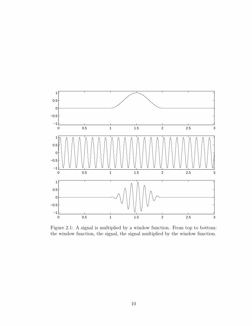
x(t)w(t− τ) (2.3)
Figure 2.1 shows the result of windowing a signal. In the top diagram, the
window has been shifted to τ = 1.5 seconds. The middle diagram shows an
8 Hz sine wave and the bottom diagram shows the windowed signal; it is the
result of multiplying the window and the sine wave. Only a small segment of
the windowed signal is nonzero, so the Fourier Transform of this signal will give
the frequency information near 1.5 seconds.
9
0 0.5 1 1.5 2 2.5 3−1
−0.5
0
0.5
1
0 0.5 1 1.5 2 2.5 3−1
−0.5
0
0.5
1
0 0.5 1 1.5 2 2.5 3−1
−0.5
0
0.5
1
Figure 2.1: A signal is multiplied by a window function. From top to bottom:the window function, the signal, the signal multiplied by the window function.
10
Plugging the product in 2.3 into the equation for the Fourier Transform (2.2)
gives the equation for the Short-Time Fourier Transform (STFT) (2.4).
XSTFT (τ, ω) =∫
x(t)w(t− τ)e−iωtdt (2.4)
The Fourier Transform of a product of two functions results in the convolu-
tion of the Fourier Transforms of the two functions. The consequences of this
will be shown in detail later, but essentially, the duration and shape of the win-
dow affect the representation created by the STFT because the spectrum of the
window is convolved with the spectrum of the signal.
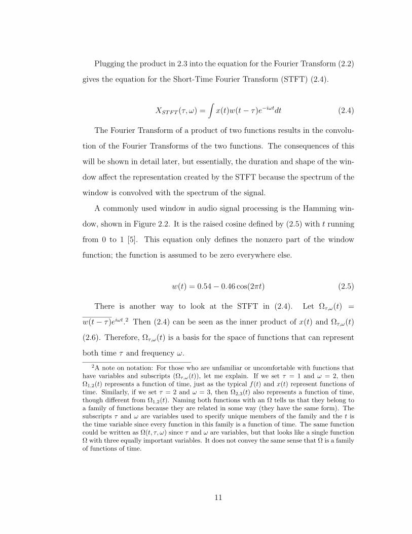
A commonly used window in audio signal processing is the Hamming win-
dow, shown in Figure 2.2. It is the raised cosine defined by (2.5) with t running
from 0 to 1 [5]. This equation only defines the nonzero part of the window
function; the function is assumed to be zero everywhere else.
w(t) = 0.54− 0.46 cos(2πt) (2.5)
There is another way to look at the STFT in (2.4). Let Ωτ,ω(t) =
w(t− τ)eiωt.2 Then (2.4) can be seen as the inner product of x(t) and Ωτ,ω(t)
(2.6). Therefore, Ωτ,ω(t) is a basis for the space of functions that can represent
both time τ and frequency ω.
2A note on notation: For those who are unfamiliar or uncomfortable with functions thathave variables and subscripts (Ωτ,ω(t)), let me explain. If we set τ = 1 and ω = 2, thenΩ1,2(t) represents a function of time, just as the typical f(t) and x(t) represent functions oftime. Similarly, if we set τ = 2 and ω = 3, then Ω2,3(t) also represents a function of time,though different from Ω1,2(t). Naming both functions with an Ω tells us that they belong toa family of functions because they are related in some way (they have the same form). Thesubscripts τ and ω are variables used to specify unique members of the family and the t isthe time variable since every function in this family is a function of time. The same functioncould be written as Ω(t, τ, ω) since τ and ω are variables, but that looks like a single functionΩ with three equally important variables. It does not convey the same sense that Ω is a familyof functions of time.
11
0 0.1 0.2 0.3 0.4 0.5 0.6 0.7 0.8 0.9 10
0.1
0.2
0.3
0.4
0.5
0.6
0.7
0.8
0.9
1
Figure 2.2: A Hamming window.
XSTFT (τ, ω) =∫
x(t)w(t− τ)e−iωtdt
=∫
x(t)w(t− τ)eiωtdt
=∫
x(t)Ωτ,ω(t)dt (2.6)
In (2.4), the window function w(t) does not depend on frequency. In other
words, the same window function is used to evaluate every frequency. Since
the window function does not change with frequency, the frequency resolution
of the STFT does not change with frequency. This also implies that the time
resolution does not change with frequency. Therefore, the choice of a window
function determines both the frequency resolution and the time resolution for
the entire representation.
The frequency of a pure tone is inversely related to the period of the wave-
form. A single period of a pure tone completely describes its shape for all time,
so a pure tone at 10 Hz is described in 1/10 of a second and a pure tone at 1000
12
Hz is described in 1/1000 of a second. Therefore, it takes longer to describe low
frequencies than it takes to describe high frequencies. This relates to the length
of the window function in the STFT because short windows might not be long
enough to capture a full period of low frequencies. If a longer window is used,
it becomes difficult to locate when a high frequency occurred.
These difficulties suggest varying the window size with frequency. Long
duration windows can be used to capture low frequencies and short duration
windows can be used to capture high frequencies. Since the frequency reso-
lution changes over the representation, the time resolution also changes; high
frequencies will be more localized in time than low frequencies. This idea is
the fundamental difference between the Short-Time Fourier Transform and the
Wavelet Transform.
2.3 Wavelet Transform
The Wavelet Transform makes the window length inversely proportional
to the frequency [6]. In other words, low frequencies are analyzed with long
windows and high frequencies are analyzed with short windows. This is often
termed a multiresolution, since the frequency resolution and the time resolu-
tion change over the representation. Although the idea of analyzing signals at
different resolutions has existed since the beginning of the century, it was only
recently that Grossman, Meyer, and Morlet created a general multiresolution
theory known as Wavelet Theory [7].
The Wavelet Transform uses a set of basis functions obtained by dilations,
contractions, and shifts of a unique function called the “wavelet prototype.”
The effect of scaling the wavelet prototype is similar to changing the size of
window in the STFT. Shifting the wavelet in time is the same as shifting the
window in the STFT. If the input signal x(t) is continuous and the time and
scale parameters are continuous, the transform is called the Continuous Wavelet
13
−5 0 5−1
−0.5
0
0.5
1
−5 0 5−1
−0.5
0
0.5
1
−5 0 5−1
−0.5
0
0.5
1
−5 0 5−1
−0.5
0
0.5
1
−5 0 5−1
−0.5
0
0.5
1
−5 0 5−1
−0.5
0
0.5
1
Figure 2.3: Shifted and scaled wavelets. By column, the wavelets are eithershifted by 0 seconds or 1 second. By row, the wavelets are either scaled by afactor of 1, 1.5, or 0.5.
Transform (CWT).
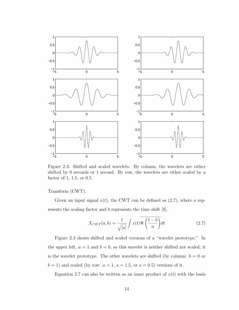
Given an input signal x(t), the CWT can be defined as (2.7), where a rep-
resents the scaling factor and b represents the time shift [8].
XCWT (a, b) =1√|a|
∫x(t)Ψ
(t− b
a
)dt (2.7)
Figure 2.3 shows shifted and scaled versions of a “wavelet prototype.” In
the upper left, a = 1 and b = 0, so this wavelet is neither shifted nor scaled; it
is the wavelet prototype. The other wavelets are shifted (by column: b = 0 or
b = 1) and scaled (by row: a = 1, a = 1.5, or a = 0.5) versions of it.
Equation 2.7 can also be written as an inner product of x(t) with the basis
14
function Ψa,b(t). This makes the similarity between the STFT in (2.6) and the
CWT in (2.8) clear. The STFT is an inner product of x(t) with Ωτ,ω(t) and the
CWT is an inner product of x(t) with Ψa,b(t). The differences between the two
transforms come directly from the differences between the two families of basis
functions. This will be covered in detail in the next section.
XCWT (a, b) =∫
x(t)Ψa,b(t)dt (2.8)
where
Ψa,b(t) =1√|a|
Ψ
(t− b
a
)(2.9)
In (2.9), as a becomes large, the basis function Ψa,b(t) stretches and is able
to analyze the low-frequency components of the signal. As a becomes small,
the basis function Ψa,b(t) contracts and is able to analyze the high frequency
components of the signal. The factor 1/√|a| in (2.9) and (2.7) guarantees energy
normalization [9].
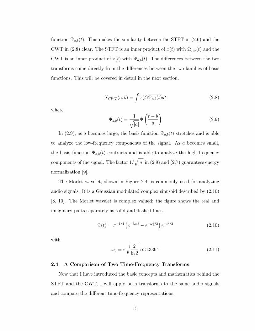
The Morlet wavelet, shown in Figure 2.4, is commonly used for analyzing
audio signals. It is a Gaussian modulated complex sinusoid described by (2.10)
[8, 10]. The Morlet wavelet is complex valued; the figure shows the real and
imaginary parts separately as solid and dashed lines.
Ψ(t) = π−1/4(e−iω0t − e−ω2
0/2)e−t2/2 (2.10)
with
ω0 = π
√2
ln 2≈ 5.3364 (2.11)
2.4 A Comparison of Two Time-Frequency Transforms
Now that I have introduced the basic concepts and mathematics behind the
STFT and the CWT, I will apply both transforms to the same audio signals
and compare the different time-frequency representations.
15
−4 −3 −2 −1 0 1 2 3 4−1
−0.5
0
0.5
1
−4 −3 −2 −1 0 1 2 3 4−1
−0.5
0
0.5
1
Figure 2.4: The Morlet wavelet. The real part is shown as a solid line and theimaginary part is shown as a dashed line.
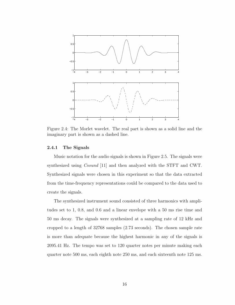
2.4.1 The Signals
Music notation for the audio signals is shown in Figure 2.5. The signals were
synthesized using Csound [11] and then analyzed with the STFT and CWT.
Synthesized signals were chosen in this experiment so that the data extracted
from the time-frequency representations could be compared to the data used to
create the signals.
The synthesized instrument sound consisted of three harmonics with ampli-
tudes set to 1, 0.8, and 0.6 and a linear envelope with a 50 ms rise time and
50 ms decay. The signals were synthesized at a sampling rate of 12 kHz and
cropped to a length of 32768 samples (2.73 seconds). The chosen sample rate
is more than adequate because the highest harmonic in any of the signals is
2095.41 Hz. The tempo was set to 120 quarter notes per minute making each
quarter note 500 ms, each eighth note 250 ms, and each sixteenth note 125 ms.
16
1. F-major arpeggio
3. Chord Progression
2. G-major Scale
Figure 2.5: Music notation for the test signals. The F-major arpeggio, G-majorscale, and chord progression were synthesized in Csound.
2.4.2 Analysis Techniques
The time-frequency representations of the audio signals were computed in
MATLAB with an optimized version of the Time-Frequency Toolbox for Matlab
[12]. All the time-frequency plots show time in seconds on the horizontal axis
and frequency in Hertz on the vertical axis. Amplitude in decibels is shown by
the darkness of the pixels from white to black.
To compare the time-frequency representations, I developed specialized
MATLAB functions to measure the center frequency, frequency width, start
time, and duration of the harmonics. Figure 2.6 shows how these values were
calculated for this experiment. For center frequency, I used parabolic interpola-
tion in the frequency domain (Appendix B describes this technique in detail). I
measured frequency width by finding the interval, or ratio, between the frequen-
cies of the two points that were 3 dB down in amplitude from the amplitude of
the center frequency.
The start time of a harmonic was calculated by searching for a strong rise
17
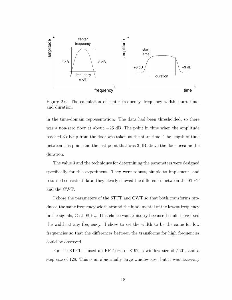
ampl
itude
frequency
centerfrequency
-3 dB-3 dB
frequencywidth
ampl
itude
time
+3 dB
duration
+3 dB
starttime
Figure 2.6: The calculation of center frequency, frequency width, start time,and duration.
in the time-domain representation. The data had been thresholded, so there
was a non-zero floor at about −26 dB. The point in time when the amplitude
reached 3 dB up from the floor was taken as the start time. The length of time
between this point and the last point that was 3 dB above the floor became the
duration.
The value 3 and the techniques for determining the parameters were designed
specifically for this experiment. They were robust, simple to implement, and
returned consistent data; they clearly showed the differences between the STFT
and the CWT.
I chose the parameters of the STFT and CWT so that both transforms pro-
duced the same frequency width around the fundamental of the lowest frequency
in the signals, G at 98 Hz. This choice was arbitrary because I could have fixed
the width at any frequency. I chose to set the width to be the same for low
frequencies so that the differences between the transforms for high frequencies
could be observed.
For the STFT, I used an FFT size of 8192, a window size of 5601, and a
step size of 128. This is an abnormally large window size, but it was necessary
18
to make the STFT have the same frequency width around 98 Hz as the CWT.
This, of course, greatly affects the time resolution of the transform, but I was
more interested in the trends of the data gathered from the representations than
the actual values.
The step size determined the number of columns in the time-frequency rep-
resentation. Since the signals were all 32768 samples long, the resulting repre-
sentations had 256 columns. There were 8192 rows, so the size of the STFT
representation was 2,097,152 complex values. I converted the complex-valued
data into magnitudes for simplicity.
I calculated the CWT from 12 Hz to 6000 Hz (0.001 to 0.5 in normalized
frequency) at 512 logarithmically spaced frequencies. The ‘wave’ parameter—
which corresponds to half length of the Morlet wavelet at coarsest scale—was
set to 70. The step size was set to 128 to make the CWT representation have
the same number of columns as the STFT representation. The total size was
much smaller, however, 131,072 complex values or one sixteenth (6.25%) of the
size of the STFT matrix. As in the STFT, the complex-values were converted
to magnitudes.
The time-frequency representations were thresholded by 5%. In other words,
any point less than 5% of the maximum value of the matrix was set to 5% of
the maximum value, creating a non-zero floor for the matrix. The magnitudes
were then converted to dB (20 log10(x)).
2.4.3 Results
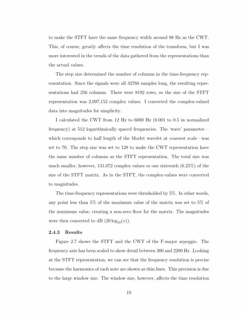
Figure 2.7 shows the STFT and the CWT of the F-major arpeggio. The
frequency axis has been scaled to show detail between 300 and 2200 Hz. Looking
at the STFT representation, we can see that the frequency resolution is precise
because the harmonics of each note are shown as thin lines. This precision is due
to the large window size. The window size, however, affects the time resolution
19
(a) STFT of the arpeggio (b) CWT of the arpeggio
Figure 2.7: The time-frequency representations of signal 1, the F-major arpeg-gio.
and all the harmonics in the plot are equally overlapped by approximately 25%.
The harmonics in Figure 2.7(b) are represented by thicker lines than those
in Figure 2.7(a), so the frequency width of the CWT is not as precise as that
of the STFT. The higher harmonics are also thicker than the lower harmonics.
The loss of frequency resolution for high frequencies results in a gain of time
resolution and therefore, the amount of overlap decreases as frequency increases.
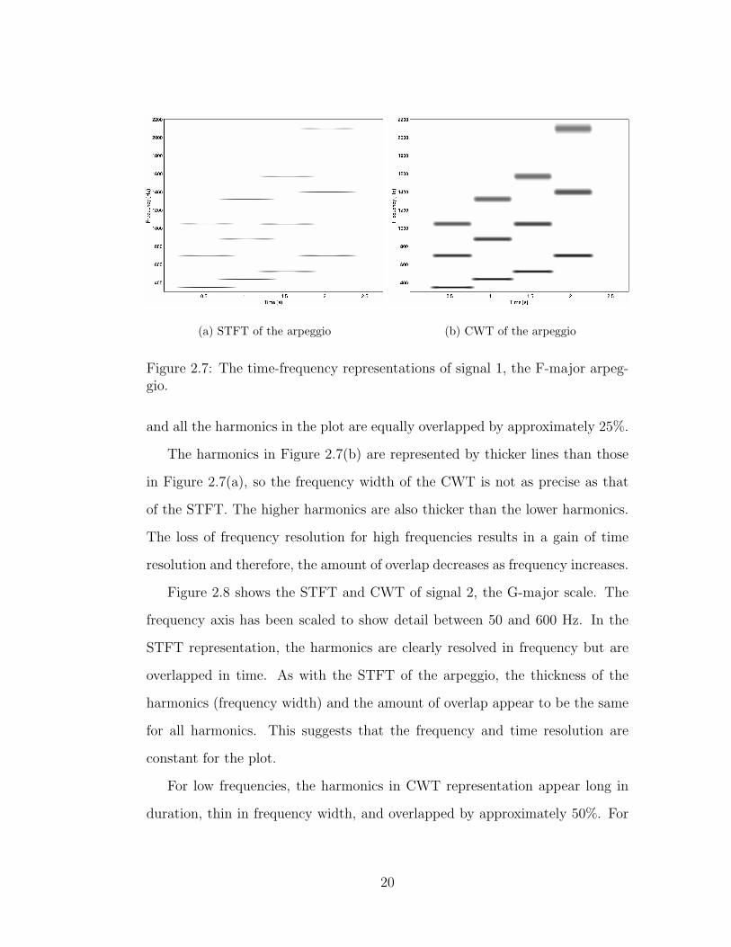
Figure 2.8 shows the STFT and CWT of signal 2, the G-major scale. The
frequency axis has been scaled to show detail between 50 and 600 Hz. In the
STFT representation, the harmonics are clearly resolved in frequency but are
overlapped in time. As with the STFT of the arpeggio, the thickness of the
harmonics (frequency width) and the amount of overlap appear to be the same
for all harmonics. This suggests that the frequency and time resolution are
constant for the plot.
For low frequencies, the harmonics in CWT representation appear long in
duration, thin in frequency width, and overlapped by approximately 50%. For
20
(a) STFT of the scale (b) CWT of the scale
Figure 2.8: The time-frequency representations of signal 2, the G-major scale.
high frequencies, the harmonics appear thick in frequency width, short in dura-
tion, and separated in time. Therefore, frequency and time resolution vary over
the plot.
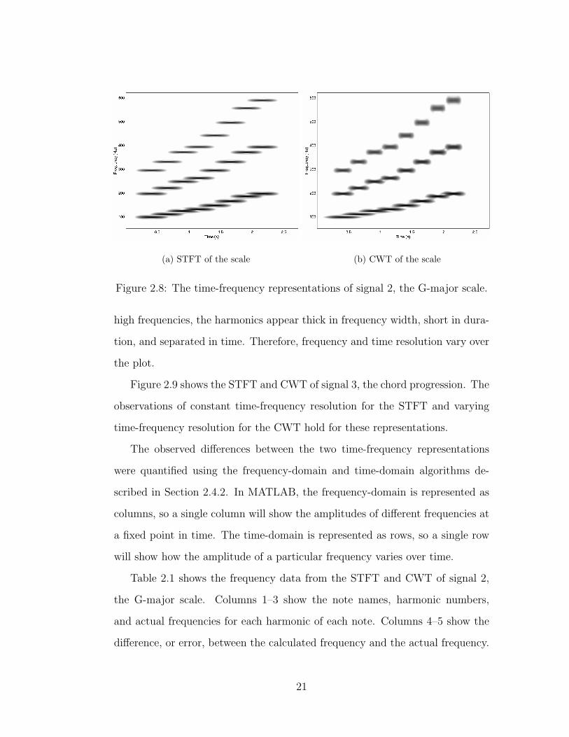
Figure 2.9 shows the STFT and CWT of signal 3, the chord progression. The
observations of constant time-frequency resolution for the STFT and varying
time-frequency resolution for the CWT hold for these representations.
The observed differences between the two time-frequency representations
were quantified using the frequency-domain and time-domain algorithms de-
scribed in Section 2.4.2. In MATLAB, the frequency-domain is represented as
columns, so a single column will show the amplitudes of different frequencies at
a fixed point in time. The time-domain is represented as rows, so a single row
will show how the amplitude of a particular frequency varies over time.
Table 2.1 shows the frequency data from the STFT and CWT of signal 2,
the G-major scale. Columns 1–3 show the note names, harmonic numbers,
and actual frequencies for each harmonic of each note. Columns 4–5 show the
difference, or error, between the calculated frequency and the actual frequency.
21
(a) STFT of the chord progression (b) CWT of the chord progression
Figure 2.9: The time-frequency representations of signal 3, the chord progres-sion.
Columns 6–7 show the calculated frequency width. All the values in the table
are in cents (100 cents is a semitone).
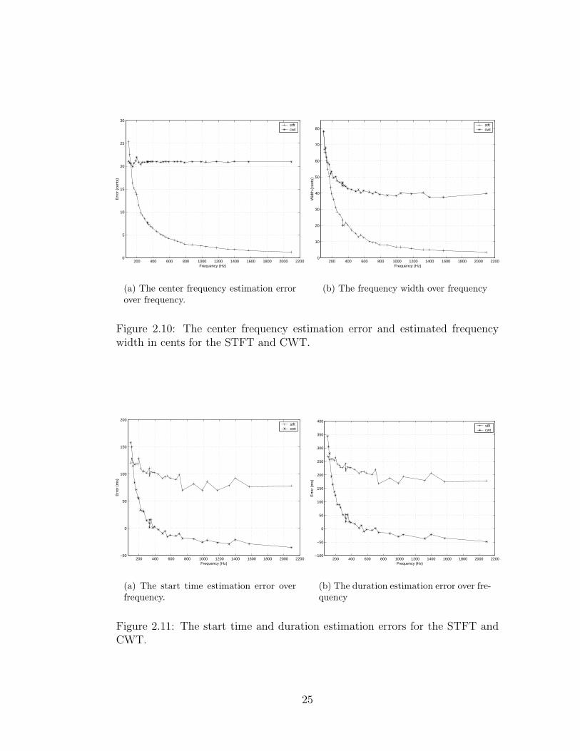
The center frequencies calculated from the STFT representation get closer
to the actual frequencies as frequency increases because the error, in cents,
decreases. For the CWT, the error is almost constant, at 20 cents, over the
entire range of frequencies. Figure 2.10(a) shows the center frequency error for
both transforms over frequency. Quantified data from all three test signals was
used to generate the figure and a single outlier was removed.
The frequency width extracted from both representations initially decreases
as frequency increases. Above 500 Hz, the frequency width of the CWT is close
to constant while the frequency width of the STFT continues to decrease. This
relationship is shown in Figure 2.10(b). Data from all three signals was used to
generate the figure.
Table 2.2 shows the quantified time data from the STFT and CWT of the
G-major scale. Columns 1–3 show the note names, harmonic numbers, and
actual start times for each harmonic of each note. Columns 4–5 show the
22
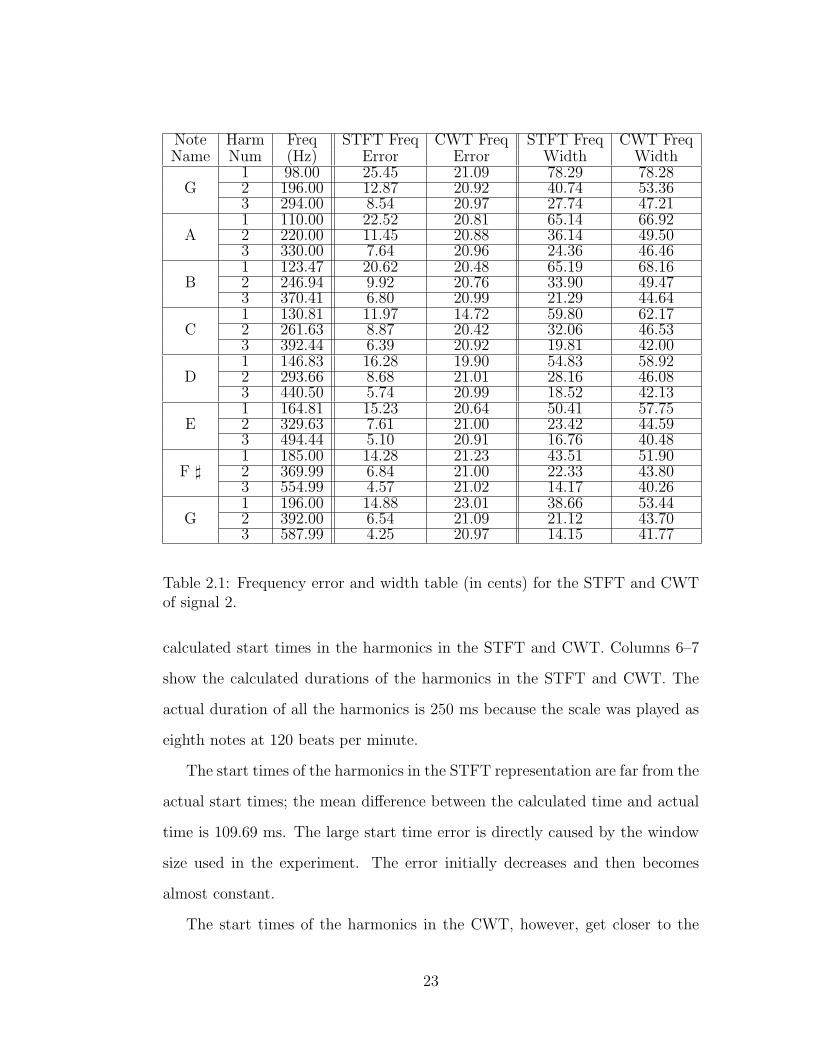
Note Harm Freq STFT Freq CWT Freq STFT Freq CWT FreqName Num (Hz) Error Error Width Width
1 98.00 25.45 21.09 78.29 78.28G 2 196.00 12.87 20.92 40.74 53.36
3 294.00 8.54 20.97 27.74 47.211 110.00 22.52 20.81 65.14 66.92
A 2 220.00 11.45 20.88 36.14 49.503 330.00 7.64 20.96 24.36 46.461 123.47 20.62 20.48 65.19 68.16
B 2 246.94 9.92 20.76 33.90 49.473 370.41 6.80 20.99 21.29 44.641 130.81 11.97 14.72 59.80 62.17
C 2 261.63 8.87 20.42 32.06 46.533 392.44 6.39 20.92 19.81 42.001 146.83 16.28 19.90 54.83 58.92
D 2 293.66 8.68 21.01 28.16 46.083 440.50 5.74 20.99 18.52 42.131 164.81 15.23 20.64 50.41 57.75
E 2 329.63 7.61 21.00 23.42 44.593 494.44 5.10 20.91 16.76 40.481 185.00 14.28 21.23 43.51 51.90
F ] 2 369.99 6.84 21.00 22.33 43.803 554.99 4.57 21.02 14.17 40.261 196.00 14.88 23.01 38.66 53.44
G 2 392.00 6.54 21.09 21.12 43.703 587.99 4.25 20.97 14.15 41.77
Table 2.1: Frequency error and width table (in cents) for the STFT and CWTof signal 2.
calculated start times in the harmonics in the STFT and CWT. Columns 6–7
show the calculated durations of the harmonics in the STFT and CWT. The
actual duration of all the harmonics is 250 ms because the scale was played as
eighth notes at 120 beats per minute.
The start times of the harmonics in the STFT representation are far from the
actual start times; the mean difference between the calculated time and actual
time is 109.69 ms. The large start time error is directly caused by the window
size used in the experiment. The error initially decreases and then becomes
almost constant.
The start times of the harmonics in the CWT, however, get closer to the
23
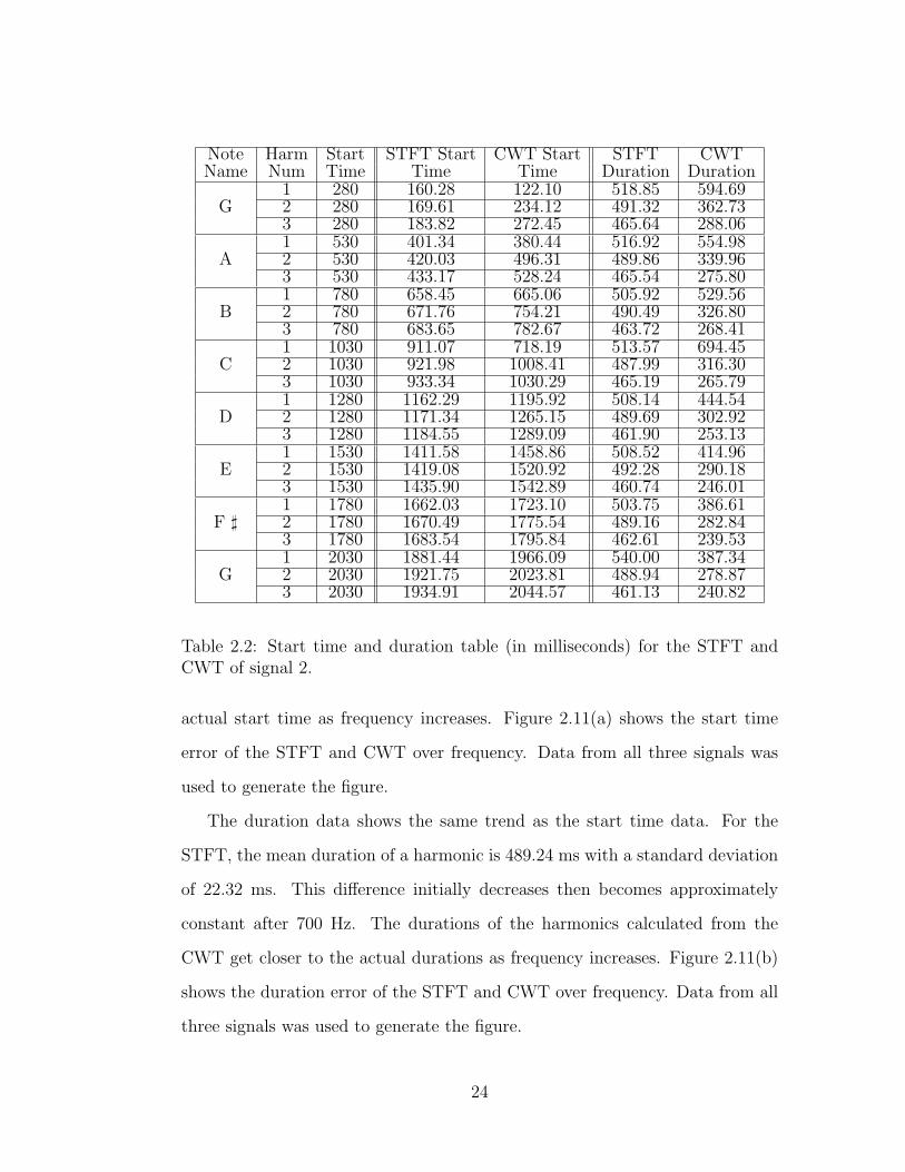
Note Harm Start STFT Start CWT Start STFT CWTName Num Time Time Time Duration Duration
1 280 160.28 122.10 518.85 594.69G 2 280 169.61 234.12 491.32 362.73
3 280 183.82 272.45 465.64 288.061 530 401.34 380.44 516.92 554.98
A 2 530 420.03 496.31 489.86 339.963 530 433.17 528.24 465.54 275.801 780 658.45 665.06 505.92 529.56
B 2 780 671.76 754.21 490.49 326.803 780 683.65 782.67 463.72 268.411 1030 911.07 718.19 513.57 694.45
C 2 1030 921.98 1008.41 487.99 316.303 1030 933.34 1030.29 465.19 265.791 1280 1162.29 1195.92 508.14 444.54
D 2 1280 1171.34 1265.15 489.69 302.923 1280 1184.55 1289.09 461.90 253.131 1530 1411.58 1458.86 508.52 414.96
E 2 1530 1419.08 1520.92 492.28 290.183 1530 1435.90 1542.89 460.74 246.011 1780 1662.03 1723.10 503.75 386.61
F ] 2 1780 1670.49 1775.54 489.16 282.843 1780 1683.54 1795.84 462.61 239.531 2030 1881.44 1966.09 540.00 387.34
G 2 2030 1921.75 2023.81 488.94 278.873 2030 1934.91 2044.57 461.13 240.82
Table 2.2: Start time and duration table (in milliseconds) for the STFT andCWT of signal 2.
actual start time as frequency increases. Figure 2.11(a) shows the start time
error of the STFT and CWT over frequency. Data from all three signals was
used to generate the figure.
The duration data shows the same trend as the start time data. For the
STFT, the mean duration of a harmonic is 489.24 ms with a standard deviation
of 22.32 ms. This difference initially decreases then becomes approximately
constant after 700 Hz. The durations of the harmonics calculated from the
CWT get closer to the actual durations as frequency increases. Figure 2.11(b)
shows the duration error of the STFT and CWT over frequency. Data from all
three signals was used to generate the figure.
24
200 400 600 800 1000 1200 1400 1600 1800 2000 22000
5
10
15
20
25
30
Frequency (Hz)
Err
or (
cent
s)
stftcwt
(a) The center frequency estimation errorover frequency.
200 400 600 800 1000 1200 1400 1600 1800 2000 22000
10
20
30
40
50
60
70
80
Frequency (Hz)
Wid
th (
cent
s)
stftcwt
(b) The frequency width over frequency
Figure 2.10: The center frequency estimation error and estimated frequencywidth in cents for the STFT and CWT.
200 400 600 800 1000 1200 1400 1600 1800 2000 2200−50
0
50
100
150
200
Frequency (Hz)
Err
or (
ms)
stftcwt
(a) The start time estimation error overfrequency.
200 400 600 800 1000 1200 1400 1600 1800 2000 2200−100
−50
0
50
100
150
200
250
300
350
400
Frequency (Hz)
Err
or (
ms)
stftcwt
(b) The duration estimation error over fre-quency
Figure 2.11: The start time and duration estimation errors for the STFT andCWT.
25
2.4.4 Conclusions
The Short-Time Fourier Transform and the Continuous Wavelet Transform
were applied to the same audio signals and the resulting time-frequency repre-
sentations were compared. The results above display the important difference
between the two transforms. If the frequency resolution is fixed at a particular
frequency for both transforms, the CWT will have better time resolution above
that frequency and better frequency resolution below that frequency than the
STFT. Of course, this improvement comes at the expense of the frequency reso-
lution for high frequencies and the time resolution for low frequencies. In other
words, the time resolution is fixed for the STFT and variable for the CWT.
A potential advantage of the CWT is the size of the time-frequency represen-
tation. For the signals above, the CWT produced representations with 131,072
complex numbers. The STFT produced representations with 2,097,152 complex
numbers. In other words, an STFT with the same low frequency response as a
CWT will produce a representation sixteen times larger than the representation
produced by the CWT.
The STFT has two significant advantages over the CWT. Since the time
resolution is fixed over the entire frequency range, synchrony in the onsets of
harmonics can be detected. This is important for determining if harmonics
belong to a particular sound; common onsets suggest that harmonics belong
together.
The other advantage is computational speed. The FFT, and therefore the
STFT, is an optimized and efficient algorithm. On most computers, the STFT of
a signal can be quickly calculated. The CWT, however, relies on convolutions
and is an order of magnitude less efficient than the STFT. Computing the
convolutions in the frequency domain speeds up the CWT dramatically, but
it still cannot compete with the STFT. In practice, dyadic Discrete Wavelet
26

Transforms are often used to create time-scale representations because there
are fast algorithms available. Extracting time and frequency information from
these representations is a possibility for further study.
27
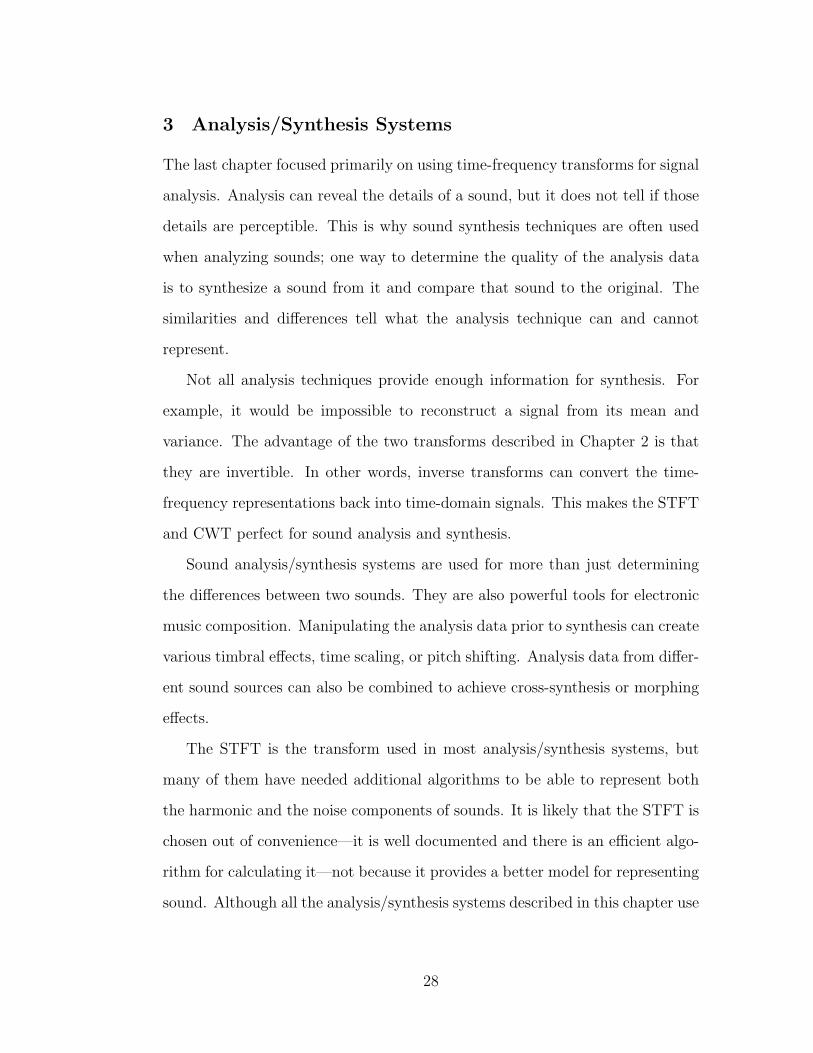
3 Analysis/Synthesis Systems
The last chapter focused primarily on using time-frequency transforms for signal
analysis. Analysis can reveal the details of a sound, but it does not tell if those
details are perceptible. This is why sound synthesis techniques are often used
when analyzing sounds; one way to determine the quality of the analysis data
is to synthesize a sound from it and compare that sound to the original. The
similarities and differences tell what the analysis technique can and cannot
represent.
Not all analysis techniques provide enough information for synthesis. For
example, it would be impossible to reconstruct a signal from its mean and
variance. The advantage of the two transforms described in Chapter 2 is that
they are invertible. In other words, inverse transforms can convert the time-
frequency representations back into time-domain signals. This makes the STFT
and CWT perfect for sound analysis and synthesis.
Sound analysis/synthesis systems are used for more than just determining
the differences between two sounds. They are also powerful tools for electronic
music composition. Manipulating the analysis data prior to synthesis can create
various timbral effects, time scaling, or pitch shifting. Analysis data from differ-
ent sound sources can also be combined to achieve cross-synthesis or morphing
effects.
The STFT is the transform used in most analysis/synthesis systems, but
many of them have needed additional algorithms to be able to represent both
the harmonic and the noise components of sounds. It is likely that the STFT is
chosen out of convenience—it is well documented and there is an efficient algo-
rithm for calculating it—not because it provides a better model for representing
sound. Although all the analysis/synthesis systems described in this chapter use
28
TF Analysis DataModification
TF SynthesisSound Sound
Figure 3.1: The phase vocoder analyzes a sound, modifies the analysis data,and synthesizes the sound.
the STFT, their designs can be extended to use any invertible time-frequency
transform. In the Spectral Modeling Toolbox, described in Chapter 4, there are
two time-frequency transforms available.
The next sections cover the sound analysis/synthesis techniques that influ-
enced the design of the Spectral Modeling Toolbox. The three systems described
below do not represent a comprehensive list of analysis/synthesis systems and
their descriptions only cover their important features; the cited references should
be used to learn more about the details of these systems.
3.1 The Phase Vocoder
The phase vocoder is widely used for time scaling and pitch shifting and the
ideas behind its design can be found in all the analysis/synthesis systems that
follow. Essentially, the phase vocoder uses a Short-Time Fourier Transform
(STFT) for analysis and an Inverse Short-Time Fourier Transform (ISTFT)
for synthesis. Time scaling and pitch shifting are achieved by modifying the
analysis data prior to synthesis [13].
On a conceptual level, the phase vocoder is the system shown in Figure 3.1.
The analysis stage uses a transform to decompose a sound onto a time-frequency
basis. The result is a set of data that describes the evolution of a sound’s
frequency components over time.
This system assumes that the time-frequency transform is able to represent
important features in the signal. In the case of the phase vocoder, the transform
is the STFT, so the sound is described in terms of windowed sinusoids. The
29
frequencies of the sinusoids are all multiples of Fs/N , where Fs is the sampling
frequency and N is the DFT size. In other words, the phase vocoder consid-
ers all frequency samples of the DFT to be equally important and a sound is
synthesized using the data for all N sinusoids between 0 and Fs/2 Hz.
A sine wave model is appropriate for many sounds, especially those with
steady harmonic components. Therefore, the phase vocoder will be able to ana-
lyze, modify, and synthesize such sounds with accuracy. Sounds with transient
and noise components, however, are not easily represented by sine waves and
the phase vocoder will have difficulty representing these sounds.
The classic phase vocoder is typically used to time scale and pitch shift
sounds. To scale time, the time trajectories of the frequency components are
interpolated before synthesis. To shift pitch, the sound is first time-scaled and
then sample-rate converted to be the same duration as the original sound [13].
While time scaling and pitch shifting are the most common modifications, many
other possibilities have been designed and implemented by Christopher Penrose
in his PVNation software [14] and Eric Lyon in his PowerPV software [15].
The major problem with the phase vocoder as an analysis/synthesis system
is that the analysis stage does not reveal information specific to the sound being
analyzed; all sounds are represented by N time-varying sinusoids. Clearly, many
of those sinusoids are not necessary to characterize most sounds. For example,
harmonic sounds can be modeled using only sinusoids at integer multiples of a
fundamental frequency. McAulay and Quatieri extended the phase vocoder to
address this problem.
3.2 The McAulay-Quatieri Analysis/Synthesis Technique
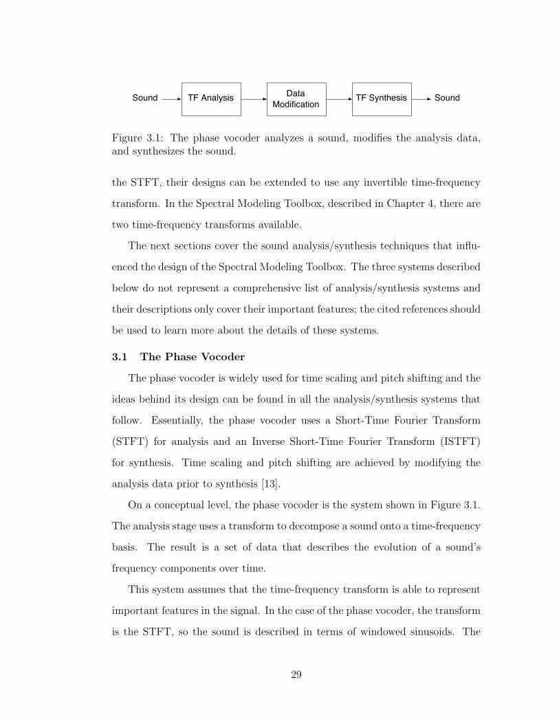
Instead of using all N frequency samples per frame, the McAulay-Quatieri
(MQ) analysis/synthesis technique isolates peaks in the spectrum since they
represent regions of high energy. Figure 3.2(a) shows the peaks of a simple
30
Frequency
Ampl
itude
(a) Detecting peaks
Time
Freq
uenc
y
(b) Forming sinusoid tracks
Figure 3.2: The McAulay-Quatieri analysis/synthesis technique forms sinusoidtracks by connecting the peaks of each frame of the STFT.
frequency spectrum. If the DFT size is 1024 (1024 frequency samples) for this
frame, then there is a significant amount of data reduction by storing only 6
of the 1024 points. Reducing the amount of analysis data provides a simpler
description of a sound and facilitates its manipulation.
The justification for reducing a complete frequency spectrum to its peaks
comes from the psychoacoustic phenomenon of masking. If two sounds are close
together in frequency, one will mask, or interfere with, the perception of the
other. Generally speaking, a loud sound will inhibit the perception of softer
sounds above it in frequency [1, p. 315]. Since peaks in a frame of the STFT
represent regions of high energy, they will mask the perception of nearby softer
frequencies.
For every frame of the STFT, the MQ technique locates the peaks and forms
tracks of peaks by connecting peaks in the current frame to nearby peaks in the
previous frame. A new track begins when there is no peak in the previous frame
that is close in frequency to a peak in the current frame. A track ends when
there is no peak in the current frame that is close enough to it in frequency.
31
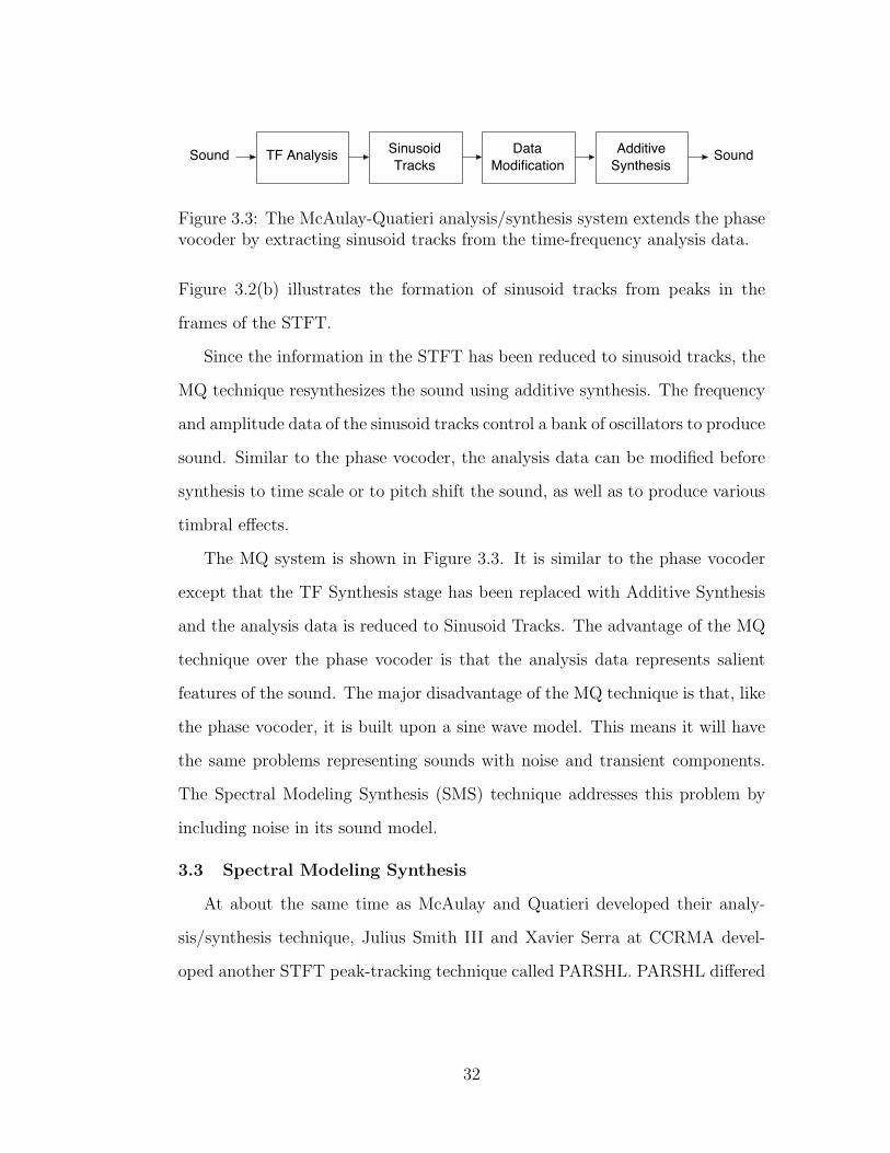
TF Analysis DataModification
AdditiveSynthesis
Sound SoundSinusoidTracks
Figure 3.3: The McAulay-Quatieri analysis/synthesis system extends the phasevocoder by extracting sinusoid tracks from the time-frequency analysis data.
Figure 3.2(b) illustrates the formation of sinusoid tracks from peaks in the
frames of the STFT.
Since the information in the STFT has been reduced to sinusoid tracks, the
MQ technique resynthesizes the sound using additive synthesis. The frequency
and amplitude data of the sinusoid tracks control a bank of oscillators to produce
sound. Similar to the phase vocoder, the analysis data can be modified before
synthesis to time scale or to pitch shift the sound, as well as to produce various
timbral effects.
The MQ system is shown in Figure 3.3. It is similar to the phase vocoder
except that the TF Synthesis stage has been replaced with Additive Synthesis
and the analysis data is reduced to Sinusoid Tracks. The advantage of the MQ
technique over the phase vocoder is that the analysis data represents salient
features of the sound. The major disadvantage of the MQ technique is that, like
the phase vocoder, it is built upon a sine wave model. This means it will have
the same problems representing sounds with noise and transient components.
The Spectral Modeling Synthesis (SMS) technique addresses this problem by
including noise in its sound model.
3.3 Spectral Modeling Synthesis
At about the same time as McAulay and Quatieri developed their analy-
sis/synthesis technique, Julius Smith III and Xavier Serra at CCRMA devel-
oped another STFT peak-tracking technique called PARSHL. PARSHL differed
32
from MQ in that interpolation on the spectral peaks was used for greater ac-
curacy and different algorithms were used for determining the beginnings and
the endings of the sinusoid tracks [16]. Essentially, both techniques solved the
problem of extracting sinusoid tracks from the STFT and they both relied on a
sine wave model of sound.
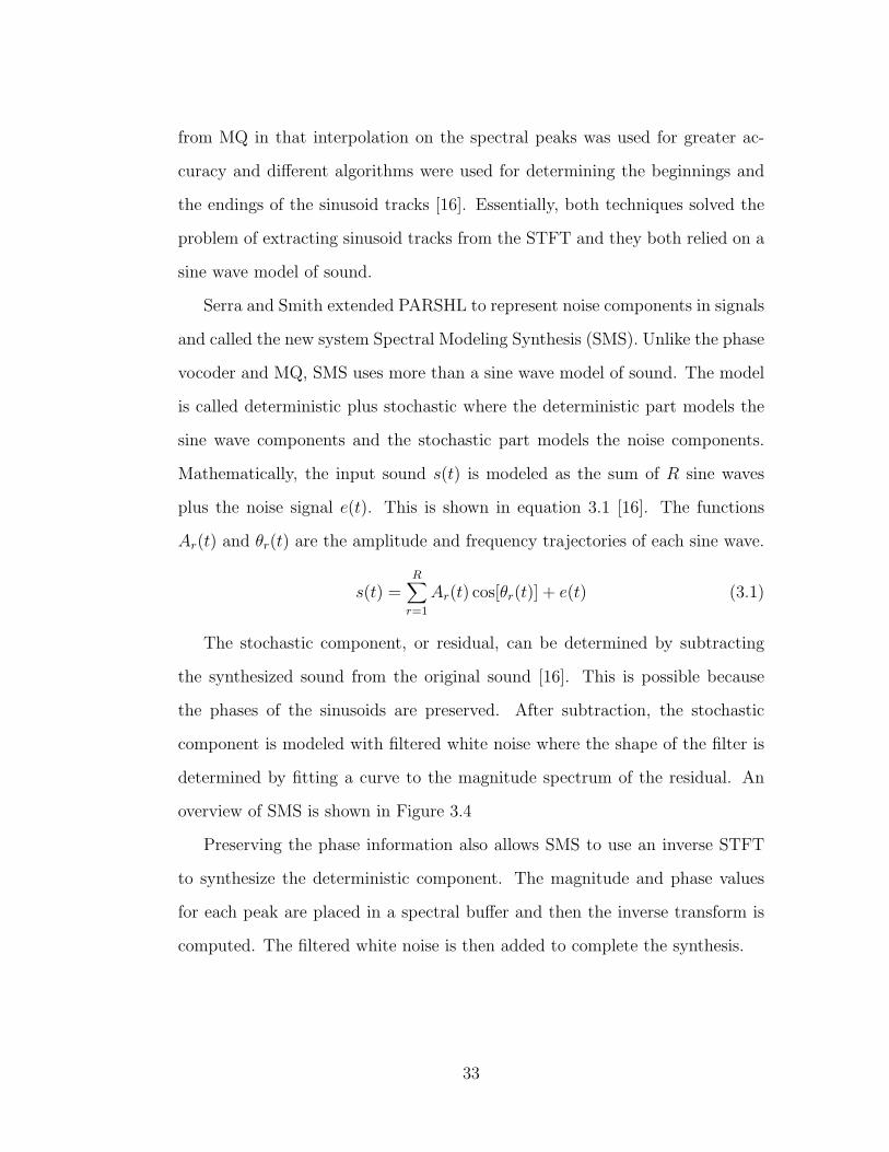
Serra and Smith extended PARSHL to represent noise components in signals
and called the new system Spectral Modeling Synthesis (SMS). Unlike the phase
vocoder and MQ, SMS uses more than a sine wave model of sound. The model
is called deterministic plus stochastic where the deterministic part models the
sine wave components and the stochastic part models the noise components.
Mathematically, the input sound s(t) is modeled as the sum of R sine waves
plus the noise signal e(t). This is shown in equation 3.1 [16]. The functions
Ar(t) and θr(t) are the amplitude and frequency trajectories of each sine wave.
s(t) =R∑
r=1
Ar(t) cos[θr(t)] + e(t) (3.1)
The stochastic component, or residual, can be determined by subtracting
the synthesized sound from the original sound [16]. This is possible because
the phases of the sinusoids are preserved. After subtraction, the stochastic
component is modeled with filtered white noise where the shape of the filter is
determined by fitting a curve to the magnitude spectrum of the residual. An
overview of SMS is shown in Figure 3.4
Preserving the phase information also allows SMS to use an inverse STFT
to synthesize the deterministic component. The magnitude and phase values
for each peak are placed in a spectral buffer and then the inverse transform is
computed. The filtered white noise is then added to complete the synthesis.
33
TF Analysis DataModification
TF SynthesisSound SoundSinusoidTracks
Residual DataModification
FilteredNoise
Figure 3.4: Spectral Modeling Synthesis can model noise and transients with aresidual signal.
While representing sound as sine waves plus noise greatly improves the qual-
ity of the synthesis, it also demonstrates that a pure sine wave model is inad-
equate for many sounds. Sound, in general, cannot be reduced to a discrete
number of sine waves and this suggests that analysis/synthesis systems should
not be limited to the sine wave basis of the STFT. In chapter 2, the CWT
was introduced as a transform that models sound using a different basis. The
Spectral Modeling Toolbox takes a generalized approach by allowing several
time-frequency transforms to be used, including the STFT and the CWT.
3.4 Design of the Spectral Modeling Toolbox
The Spectral Modeling Toolbox extends the ideas of MQ and SMS to work
with other time-frequency transforms. In addition, the framework of the Tool-
box is flexible, so many analysis/synthesis systems can be created using its
functions. Although the overall design descends from MQ and SMS, the im-
plementation differs significantly to allow the user to control any aspect of the
system. A global view of the system is shown in Figure 3.5. This rest of this
chapter will give detailed descriptions of each part of the system.
3.4.1 TF Analysis
The two functions used for time-frequency analysis were discussed in detail
in Chapter 2. Essentially, the TF analysis stage takes a sound file as input and
34
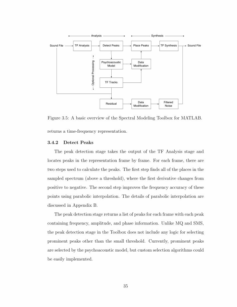
TF Analysis Detect Peaks Place Peaks TF SynthesisSound File Sound File
PsychoacousticModel
TF Tracks
Analysis Synthesis
Residual
DataModification
DataModification
FilteredNoise
Opt
iona
l Pro
cess
ing
Figure 3.5: A basic overview of the Spectral Modeling Toolbox for MATLAB.
returns a time-frequency representation.
3.4.2 Detect Peaks
The peak detection stage takes the output of the TF Analysis stage and
locates peaks in the representation frame by frame. For each frame, there are
two steps used to calculate the peaks. The first step finds all of the places in the
sampled spectrum (above a threshold), where the first derivative changes from
positive to negative. The second step improves the frequency accuracy of these
points using parabolic interpolation. The details of parabolic interpolation are
discussed in Appendix B.
The peak detection stage returns a list of peaks for each frame with each peak
containing frequency, amplitude, and phase information. Unlike MQ and SMS,
the peak detection stage in the Toolbox does not include any logic for selecting
prominent peaks other than the small threshold. Currently, prominent peaks
are selected by the psychoacoustic model, but custom selection algorithms could
be easily implemented.
35
102
103
104
0
10
20
30
40
50
60
Frequency (Hz)
Sou
nd P
ress
ure
Leve
l (dB
)
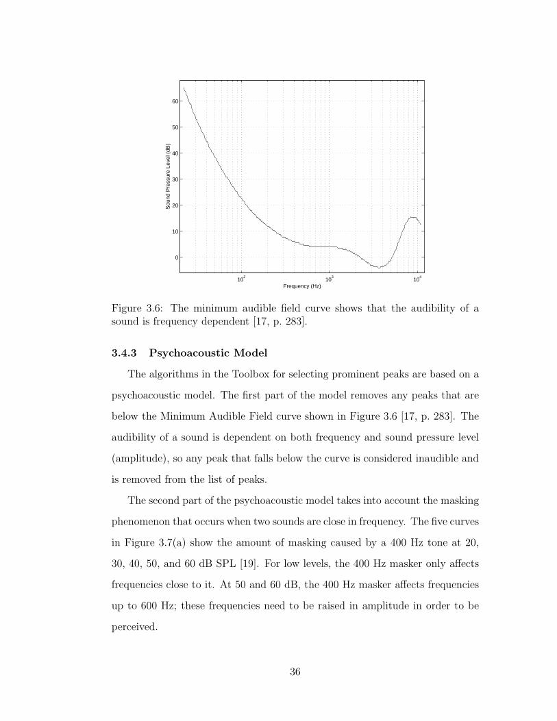
Figure 3.6: The minimum audible field curve shows that the audibility of asound is frequency dependent [17, p. 283].
3.4.3 Psychoacoustic Model
The algorithms in the Toolbox for selecting prominent peaks are based on a
psychoacoustic model. The first part of the model removes any peaks that are
below the Minimum Audible Field curve shown in Figure 3.6 [17, p. 283]. The
audibility of a sound is dependent on both frequency and sound pressure level
(amplitude), so any peak that falls below the curve is considered inaudible and
is removed from the list of peaks.
The second part of the psychoacoustic model takes into account the masking
phenomenon that occurs when two sounds are close in frequency. The five curves
in Figure 3.7(a) show the amount of masking caused by a 400 Hz tone at 20,
30, 40, 50, and 60 dB SPL [19]. For low levels, the 400 Hz masker only affects
frequencies close to it. At 50 and 60 dB, the 400 Hz masker affects frequencies
up to 600 Hz; these frequencies need to be raised in amplitude in order to be
perceived.
36
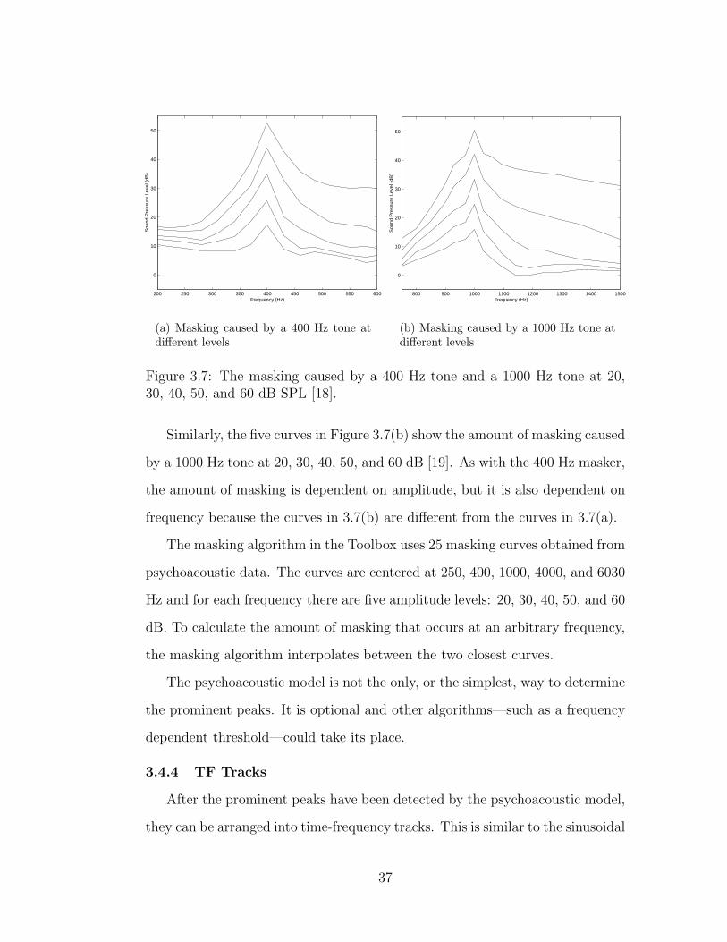
200 250 300 350 400 450 500 550 600
0
10
20
30
40
50
Frequency (Hz)
Sou
nd P
ress
ure
Leve
l (dB
)
(a) Masking caused by a 400 Hz tone atdifferent levels
800 900 1000 1100 1200 1300 1400 1500
0
10
20
30
40
50
Frequency (Hz)
Sou
nd P
ress
ure
Leve
l (dB
)
(b) Masking caused by a 1000 Hz tone atdifferent levels
Figure 3.7: The masking caused by a 400 Hz tone and a 1000 Hz tone at 20,30, 40, 50, and 60 dB SPL [18].
Similarly, the five curves in Figure 3.7(b) show the amount of masking caused
by a 1000 Hz tone at 20, 30, 40, 50, and 60 dB [19]. As with the 400 Hz masker,
the amount of masking is dependent on amplitude, but it is also dependent on
frequency because the curves in 3.7(b) are different from the curves in 3.7(a).
The masking algorithm in the Toolbox uses 25 masking curves obtained from
psychoacoustic data. The curves are centered at 250, 400, 1000, 4000, and 6030
Hz and for each frequency there are five amplitude levels: 20, 30, 40, 50, and 60
dB. To calculate the amount of masking that occurs at an arbitrary frequency,
the masking algorithm interpolates between the two closest curves.
The psychoacoustic model is not the only, or the simplest, way to determine
the prominent peaks. It is optional and other algorithms—such as a frequency
dependent threshold—could take its place.
3.4.4 TF Tracks
After the prominent peaks have been detected by the psychoacoustic model,
they can be arranged into time-frequency tracks. This is similar to the sinusoidal
37
tracks in MQ and SMS.
When using other time-frequency transforms, however, the peaks do not
represent sinusoidal components, so the tracks are technically not sinusoidal
tracks. For example, a wavelet transform would have wavelet tracks because
the basis is the set of wavelets. The track-forming concept still applies because
peaks in a time-frequency representation represent points of high time-frequency
energy. These points are connected into tracks to facilitate manipulation at later
stages.
3.4.5 Residual
The residual stage calculates the residual signal by synthesizing the TF
tracks and subtracting the synthesized signal from the original. The residual
signal was discussed in the section on SMS; it reveals the parts of the input signal
that are not easily represented by the model. The residual can be modeled with
filtered noise or used as is. It is typically added to a synthesized signal to add
realism.
3.4.6 Data Modification
As in all the analysis/synthesis systems discussed in this chapter, the analysis
data can be modified before synthesis. This allows for spectral manipulation,
time stretching, pitch scaling, cross synthesis, and other effects. The residual
signal can also be modified to enhance attacks or reduce noise in the signal.
Essentially, the functions in this stage take a type of input and return the
same type of output. A simple function, like time scaling, only needs a list
of peaks; it can take the output of the peak detection stage. More advanced
functions require TF tracks, so a TF track forming function needs to be run in
advance.
38
3.4.7 Place Peaks
The place peaks stage takes a list of peaks or a set of TF tracks as input and
generates a time-frequency representation. The process begins with an empty
spectral buffer. The amplitude and phase values for each peak are added to the
correct location in the spectral buffer. Basically, the place peaks stage does the
opposite of the detect peaks stage and prepares a spectral buffer for the inverse
transform.
3.4.8 TF Synthesis
The TF synthesis stage takes the spectral buffer and inverts it using an
inverse time-frequency transform. This produces a time-domain signal which
can be added to the residual signal to produce the final sound file.
39
4 The Spectral Modeling Toolbox
The end of the last chapter gave an overview of the Spectral Modeling Toolbox.
This chapter will present the some of the functions in the Toolbox through code
examples and diagrams. The code samples in each section assume that the
variables from the previous sections are still in memory.
4.1 Installing the Toolbox
The Spectral Modeling Toolbox can be downloaded from http://eamusic.
dartmouth.edu/~kimo/smt or http://homepage.mac.com/kimo/smt. Please
email questions, comments, and bug reports to [email protected].
The Toolbox is a tarred and gzipped folder of MATLAB files. To extract
these files on a UNIX platform, execute the command below. A folder named
SMToolbox will be created. In that folder is a README file with the latest
information and detailed installation instructions.
# tar -xzvf SMToolbox.tar.gz
To use the Toolbox, the functions need to be in your MATLAB path. Read the
README file for the list of directories and how to add them to your path.
Once the Toolbox is properly installed, the command help smt will display
the list of available functions. All the functions begin with the prefix smt_ so
that they do not conflict with functions from other toolboxes.
4.2 Reading and Writing Audio Files
The Toolbox uses MATLAB’s wavread or auread functions to read audio
files. The command below will read an audio file named filename.wav and store
it in a variable named signal. The semicolon at the end is very important:
without it, all the samples in the file will be printed to the screen.
>> signal = wavread(’filename.wav’);
40
If filename.wav is a mono file, the signal variable will be a single column vector,
and if it is a stereo file, the signal variable will be a two column matrix. In both
cases, the number of rows will be equal to the number of samples in the file.
To write audio files, use the commands wavwrite or auwrite. Typing help
on any command will show all the available options. Below, the signal vector
is written to a sound file outfile.wav with a sampling rate of 44100. On some
platforms, soundsc will play the sound at the specified sampling rate.
>> help wavwrite
>> wavwrite(signal,44100,’outfile.wav’);
>> soundsc(signal,44100);
4.3 TF Analysis and TF Synthesis
In this section, we will complete a simple analysis and synthesis of an au-
dio file. In the SoundFiles directory, there is a recording of a saxophone called
sax.wav. Use the wavread command to read the sound into the signal vari-
able and the sampling rate into the Fs variable. Take the Short-Time Fourier
Transform of the signal with hop size set to 128 samples, FFT size set to 2048
samples, and window size set to 1025 samples. The time-frequency representa-
tion is returned to the tfr variable and a time-frequency transform structure is
returned to the tfr s variable.
>> [signal,Fs] = wavread(’sax.wav’);
>> help smt_stft
>> [tfr,tfr_s] = smt_stft(signal,128,2048,1025);
The time-frequency transform structure holds information related to the time-
frequency representation. This information is used by other functions so we will
examine its contents by typing its name at the MATLAB prompt. To access any
of the fields individually, type the variable name, followed by a period, followed
by the field name (example tfr_s.N).
41
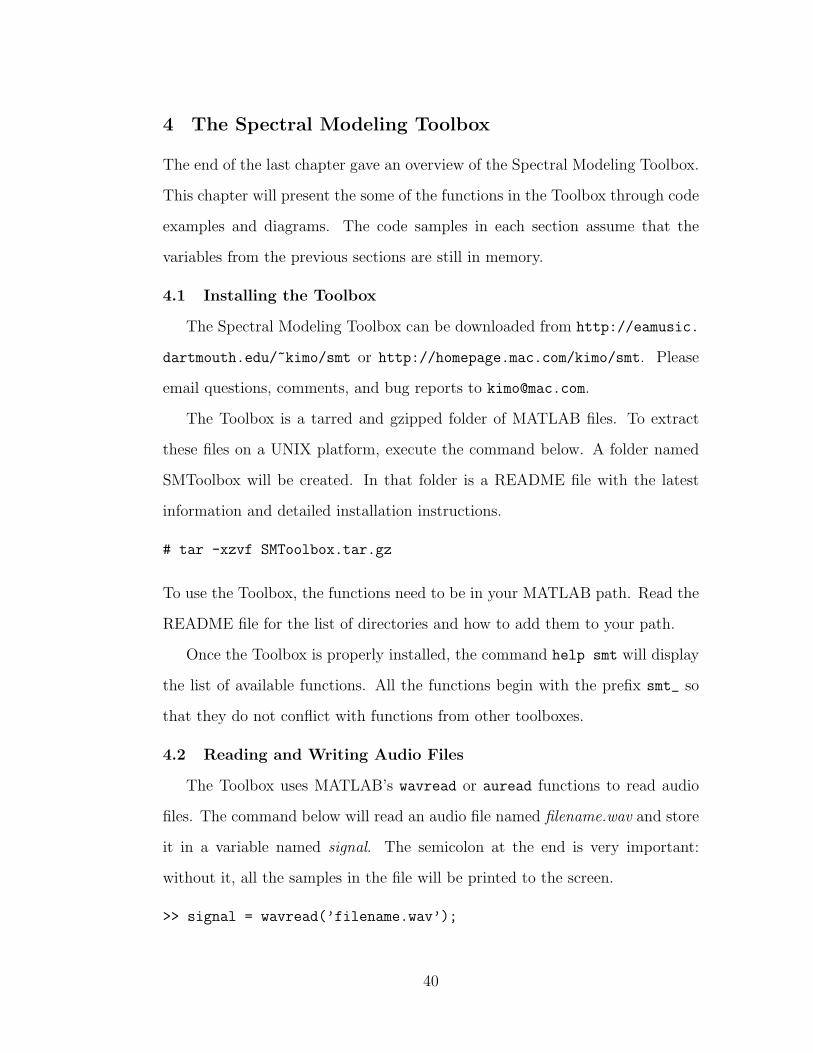
Time (ms)
Fre
quen
cy (
Hz)
STFT plot − hop:128, N:2048
100 200 300 400 500 600 700 8000
500
1000
1500
2000
2500
3000
3500
4000
4500
5000
Figure 4.1: The STFT of a saxophone note scaled to show detail between 50 to850 ms and 0 to 5000 Hz.
>> tfr_s
tfr_s =
type: ’stft’
Fs: 44100
N: 2048
max: 143.4354
w: ’hamming’
h: 1025
hop: 128
The smt_plotTFR function takes the time-frequency representation (tfr) and
the time-frequency transform structure (tfr s) to produce a plot similar to Fig-
ure 4.1. The axis command scales the x-axis to show times between 50 and
850 ms and the y-axis to show frequencies between 0 and 5000 Hz.
>> help smt_plotTFR
>> smt_plotTFR(tfr,tfr_s)
>> axis([50 850 0 5000])
42
To resynthesize the signal, use the smt_istft function. The signal can then be
listened to with soundsc or written to a file with wavwrite. The smt_istft
function normalizes the signal, so it may be louder than the original.
>> help smt_istft
>> outSignal = smt_istft(tfr,tfr_s);
>> soundsc(outSignal,44100);
>> wavwrite(outSignal,44100,’outSignal.wav’);
Before moving on, it is important to understand the format of the time-
frequency representation returned from the smt_stft function. The whos com-
mand shows all of the current variables (and their sizes), and the size command
shows the size of a particular variable.
>> whos
>> size(tfr)
ans =
2048 337
This time-frequency representation has 2048 rows and 337 columns. The
data is complex valued, so the abs and angle functions should be used to
convert the data to magnitude and phase values. In this thesis, I have been
referring to the columns of time-frequency representations as frames.
The commands below will plot the frequency content of the 100th frame as
shown in Figure 4.2. Typing tfr(:,100) tells MATLAB that we wish to look
at all the rows in column 100. To look at rows 200 to 900 of column 100 of the
tfr matrix, type the following at the prompt: tfr(200:900,100). The axis
command scales the plot to look at frequencies between 0 and 5000 Hz and
amplitude values between 0 and 1.
>> help smt_plotSpec
>> smt_plotSpec(tfr(:,100),tfr_s,0,’lin’)
>> axis([0 5000 0 1])
43
0 500 1000 1500 2000 2500 3000 3500 4000 4500 50000
0.1
0.2
0.3
0.4
0.5
0.6
0.7
0.8
0.9
1
Frequency (Hz)
Am
plitu
de (
linea
r)
Frequency Spectrum (linear scaling)
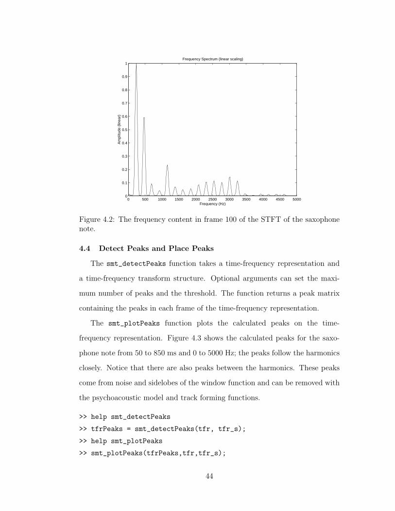
Figure 4.2: The frequency content in frame 100 of the STFT of the saxophonenote.
4.4 Detect Peaks and Place Peaks
The smt_detectPeaks function takes a time-frequency representation and
a time-frequency transform structure. Optional arguments can set the maxi-
mum number of peaks and the threshold. The function returns a peak matrix
containing the peaks in each frame of the time-frequency representation.
The smt_plotPeaks function plots the calculated peaks on the time-
frequency representation. Figure 4.3 shows the calculated peaks for the saxo-
phone note from 50 to 850 ms and 0 to 5000 Hz; the peaks follow the harmonics
closely. Notice that there are also peaks between the harmonics. These peaks
come from noise and sidelobes of the window function and can be removed with
the psychoacoustic model and track forming functions.
>> help smt_detectPeaks
>> tfrPeaks = smt_detectPeaks(tfr, tfr_s);
>> help smt_plotPeaks
>> smt_plotPeaks(tfrPeaks,tfr,tfr_s);
44
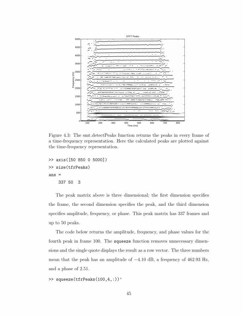
Time (ms)
Fre
quen
cy (
Hz)
STFT Peaks
100 200 300 400 500 600 700 8000
500
1000
1500
2000
2500
3000
3500
4000
4500
5000
Figure 4.3: The smt detectPeaks function returns the peaks in every frame ofa time-frequency representation. Here the calculated peaks are plotted againstthe time-frequency representation.
>> axis([50 850 0 5000])
>> size(tfrPeaks)
ans =
337 50 3
The peak matrix above is three dimensional; the first dimension specifies
the frame, the second dimension specifies the peak, and the third dimension
specifies amplitude, frequency, or phase. This peak matrix has 337 frames and
up to 50 peaks.
The code below returns the amplitude, frequency, and phase values for the
fourth peak in frame 100. The squeeze function removes unnecessary dimen-
sions and the single quote displays the result as a row vector. The three numbers
mean that the peak has an amplitude of −4.10 dB, a frequency of 462.93 Hz,
and a phase of 2.51.
>> squeeze(tfrPeaks(100,4,:))’
45
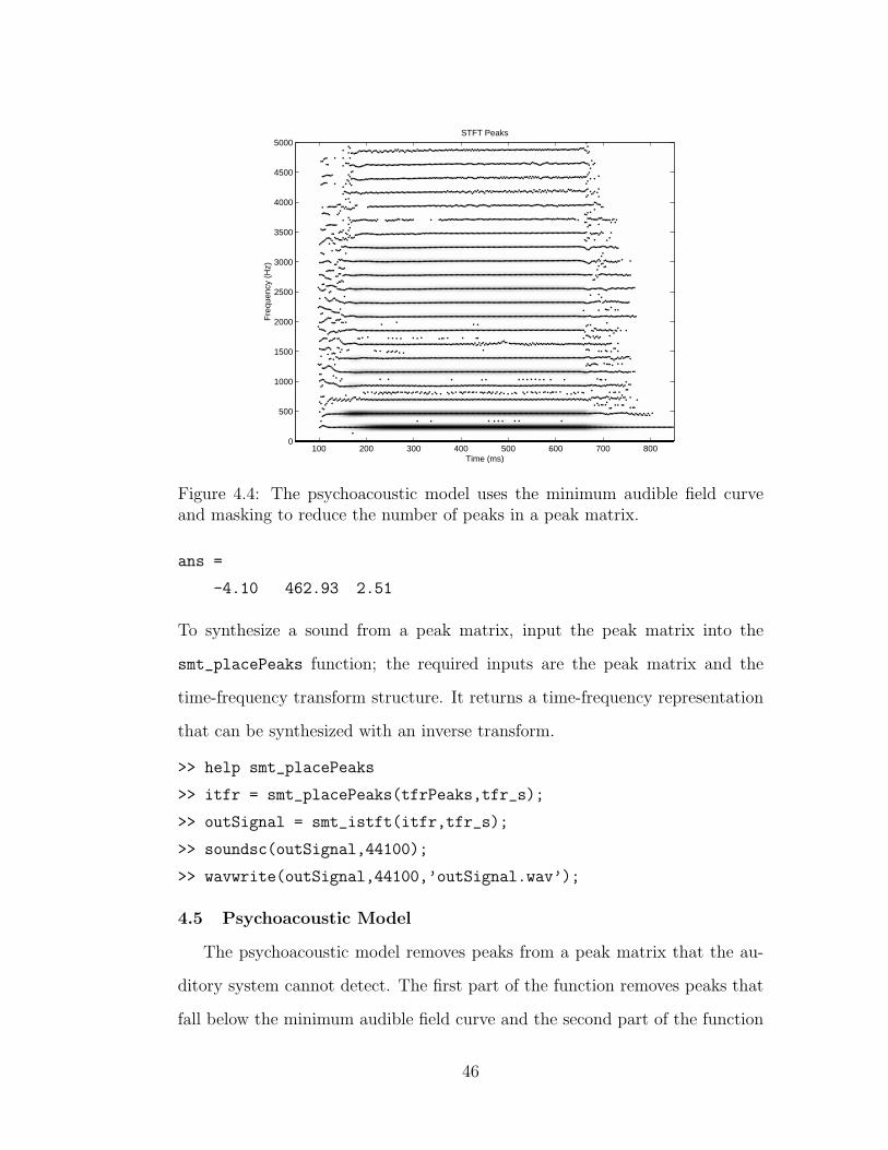
Time (ms)
Fre
quen
cy (
Hz)
STFT Peaks
100 200 300 400 500 600 700 8000
500
1000
1500
2000
2500
3000
3500
4000
4500
5000
Figure 4.4: The psychoacoustic model uses the minimum audible field curveand masking to reduce the number of peaks in a peak matrix.
ans =
-4.10 462.93 2.51
To synthesize a sound from a peak matrix, input the peak matrix into the
smt_placePeaks function; the required inputs are the peak matrix and the
time-frequency transform structure. It returns a time-frequency representation
that can be synthesized with an inverse transform.
>> help smt_placePeaks
>> itfr = smt_placePeaks(tfrPeaks,tfr_s);
>> outSignal = smt_istft(itfr,tfr_s);
>> soundsc(outSignal,44100);
>> wavwrite(outSignal,44100,’outSignal.wav’);
4.5 Psychoacoustic Model
The psychoacoustic model removes peaks from a peak matrix that the au-
ditory system cannot detect. The first part of the function removes peaks that
fall below the minimum audible field curve and the second part of the function
46
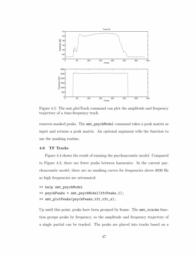
0 50 100 150 200 250 300 350−70
−60
−50
−40
−30
−20
−10
Frame
Am
plitu
de (
dB)
Track #3
0 50 100 150 200 250 300 3500
500
1000
1500
2000
2500
3000
Frame
Fre
quen
cy (
Hz)
Figure 4.5: The smt plotTrack command can plot the amplitude and frequencytrajectory of a time-frequency track.
removes masked peaks. The smt_psychModel command takes a peak matrix as
input and returns a peak matrix. An optional argument tells the function to
use the masking routine.
4.6 TF Tracks
Figure 4.4 shows the result of running the psychoacoustic model. Compared
to Figure 4.3, there are fewer peaks between harmonics. In the current psy-
choacoustic model, there are no masking curves for frequencies above 6030 Hz
so high frequencies are attenuated.
>> help smt_psychModel
>> psychPeaks = smt_psychModel(tfrPeaks,1);
>> smt_plotPeaks(psychPeaks,tfr,tfr_s);
Up until this point, peaks have been grouped by frame. The smt_tracks func-
tion groups peaks by frequency, so the amplitude and frequency trajectory of
a single partial can be tracked. The peaks are placed into tracks based on a
47
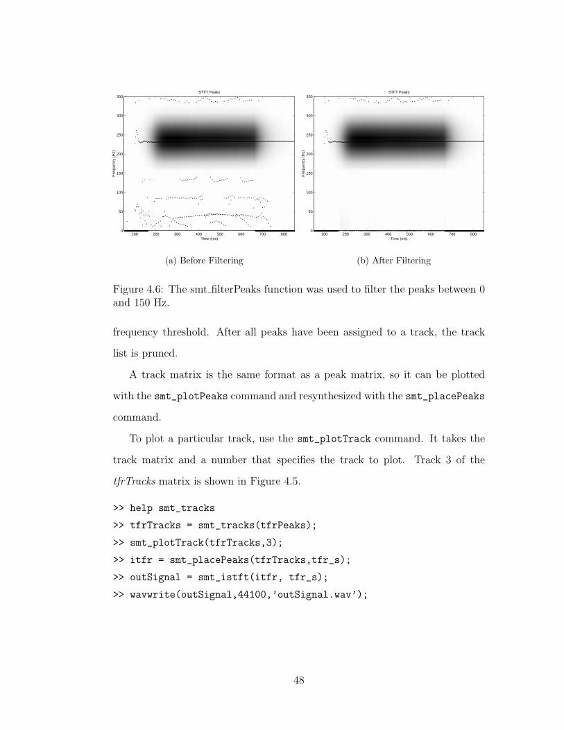
Time (ms)
Fre
quen
cy (
Hz)
STFT Peaks
100 200 300 400 500 600 700 8000
50
100
150
200
250
300
350
(a) Before Filtering
Time (ms)
Fre
quen
cy (
Hz)
STFT Peaks
100 200 300 400 500 600 700 8000
50
100
150
200
250
300
350
(b) After Filtering
Figure 4.6: The smt filterPeaks function was used to filter the peaks between 0and 150 Hz.
frequency threshold. After all peaks have been assigned to a track, the track
list is pruned.
A track matrix is the same format as a peak matrix, so it can be plotted
with the smt_plotPeaks command and resynthesized with the smt_placePeaks
command.
To plot a particular track, use the smt_plotTrack command. It takes the
track matrix and a number that specifies the track to plot. Track 3 of the
tfrTracks matrix is shown in Figure 4.5.
>> help smt_tracks
>> tfrTracks = smt_tracks(tfrPeaks);
>> smt_plotTrack(tfrTracks,3);
>> itfr = smt_placePeaks(tfrTracks,tfr_s);
>> outSignal = smt_istft(itfr, tfr_s);
>> wavwrite(outSignal,44100,’outSignal.wav’);
48
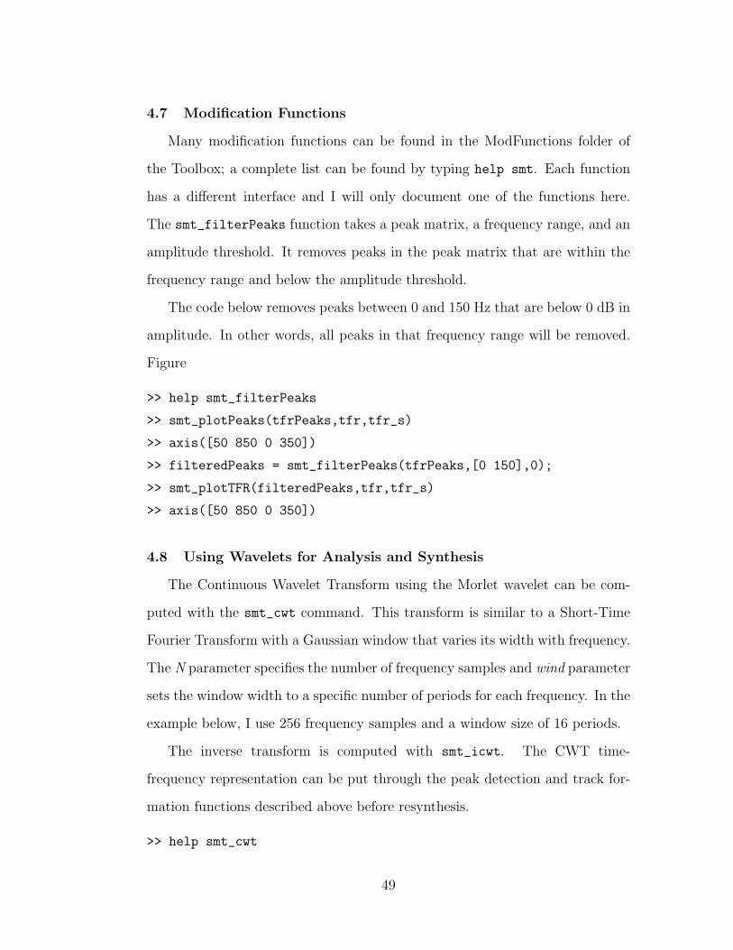
4.7 Modification Functions
Many modification functions can be found in the ModFunctions folder of
the Toolbox; a complete list can be found by typing help smt. Each function
has a different interface and I will only document one of the functions here.
The smt_filterPeaks function takes a peak matrix, a frequency range, and an
amplitude threshold. It removes peaks in the peak matrix that are within the
frequency range and below the amplitude threshold.
The code below removes peaks between 0 and 150 Hz that are below 0 dB in
amplitude. In other words, all peaks in that frequency range will be removed.
Figure
>> help smt_filterPeaks
>> smt_plotPeaks(tfrPeaks,tfr,tfr_s)
>> axis([50 850 0 350])
>> filteredPeaks = smt_filterPeaks(tfrPeaks,[0 150],0);
>> smt_plotTFR(filteredPeaks,tfr,tfr_s)
>> axis([50 850 0 350])
4.8 Using Wavelets for Analysis and Synthesis
The Continuous Wavelet Transform using the Morlet wavelet can be com-
puted with the smt_cwt command. This transform is similar to a Short-Time
Fourier Transform with a Gaussian window that varies its width with frequency.
The N parameter specifies the number of frequency samples and wind parameter
sets the window width to a specific number of periods for each frequency. In the
example below, I use 256 frequency samples and a window size of 16 periods.
The inverse transform is computed with smt_icwt. The CWT time-
frequency representation can be put through the peak detection and track for-
mation functions described above before resynthesis.
>> help smt_cwt
49
Figure 4.7: The CWT of the saxophone note.
>> [cwt, cwt_s] = smt_cwt(signal,256,16);
>> smt_plotTFR(cwt,cwt_s)
>> help smt_icwt
>> outSignal = smt_icwt(cwt,cwt_s);
50
5 Conclusions and Future Directions
The Spectral Modeling Toolbox is an environment for sound analysis, synthesis,
and research. It is designed as a foundation for algorithm development and
experimentation and the source code is available for anyone to download and
use. I hope that other people will find it useful and contribute to the project
by adding functions and improving algorithms.
The Toolbox is a learning system. I could have used existing systems to
analyze and synthesize sounds, but I chose to implement the algorithms myself
to gain a better understanding of the details. The code is heavily commented
and some of the functions favor simpler, rather than more robust, solutions.
While I would like them improved, I hope to keep some of the original algorithms
in the Toolbox for pedagogic reasons; other people may benefit from the simple
approach.
This thesis was also written favoring the simple approach. I have presented
an overview of the Toolbox and a guide for using it without going too far into
the details of the individual algorithms. Since the complete commented source
code is available, I felt no need to describe the algorithms in the body of the
thesis; the code itself and the comments are the best possible documentation.
The Spectral Modeling Toolbox is a resource for learning about sound analysis
and synthesis and I hope the approach of this thesis will provide a foundation
for further study and experimentation.
As stated in the Introduction, one of the reasons I chose to study analy-
sis/synthesis systems is because I believe they are the first step towards artifi-
cial recognition and separation of sound sources. The fundamental idea behind
the analysis stage is to transform a sound into a representation where the per-
ceptually salient features are more easily accessible. In the case of the systems
51

described in this thesis, the sounds were transformed into time-frequency repre-
sentations and the time-varying frequency content in the signal over time could
be examined. Peaks were identified as salient features (at a low level) and
extracted from the representation.
I believe the next step is to identify groups of peaks and form higher level
connections. Sinusoidal tracks are one way of doing this, but I believe there are
more general ways based on psychoacoustic theories. For example, the Gestalt
principles of grouping can be applied to auditory data. Bregman outlined many
clues that the auditory system uses to group data and an intelligent system
could use these to determine the best possible grouping for a set of peaks [2].
This requires further investigation and I believe the Spectral Modeling Toolbox
provides a decent framework for this type of research.
Those interested in sound analysis and synthesis should download the Tool-
box and try it out. I would appreciate any comments and suggestions. Based
on feedback and possibly other contributions, the design and functions in the
Toolbox may change; please read the README file for the latest information.
52
References
[1] S. Handel, Listening: An Introduction to the Perception of Auditory Events.
Cambridge, MA: The MIT Press, first ed., 1989.
[2] A. S. Bregman, Auditory Scene Analysis. Cambridge, MA: The MIT Press,
second ed., 1990.
[3] C.-T. Chen, Digital Signal Processing. New York: Oxford University Press,
Inc., first ed., 2001.
[4] D. Gabor, “Theory of communication,” Journal of the IEEE, vol. 93,
pp. 429–457, 1946.
[5] F. J. Harris, “On the use of windows for harmonic analysis with the discrete
fourier transform,” Proceedings of the IEEE, vol. 66, no. 1, pp. 51–84, 1978.
[6] P. Masri, A. Bateman, and N. Canagarajah, “A review of time-frequency
representations with application to sound/music analysis-resynthesis,” Or-
ganised Sound, vol. 2, no. 3, pp. 193–205, 1997.
[7] M. Akay and C. Mello, “Time-frequency and time-scale (wavelets) analy-
sis methods: Design and algorithms,” Smart Engineering System Design,
vol. 1, pp. 77–94, 1998.
[8] I. Daubechies, Ten Lectures on Wavelets. Philadelphia: Society for Indus-
trial and Applied Mathematics, first ed., 1992.
[9] O. Rioul and M. Vetterli, “Wavelets and signal processing,” IEEE Signal
Processing Magazine, vol. 93, pp. 14–38, 1946.
[10] R. Kronland-Martinet, “The wavelet transform for analysis, synthesis, and
53
processing of speech and music sounds,” Computer Music Journal, vol. 12,
no. 4, pp. 11–20, 1988.
[11] B. Vercoe and et al., “Csound.” http://www.csound.org, 2002.
[12] F. Auger, P. Flandrin, O. Lemoine, and P. Goncalves, “Time-frequency
toolbox for matlab.” http://crttsn.univ-nantes.fr/~auger/tftb.
html, 1999.
[13] M. Dolson, “The phase vocoder: A tutorial,” Computer Music Journal,
vol. 10, no. 4, pp. 14–28, 1986.
[14] C. Penrose, “PVNation.” http://www.sfc.keio.ac.jp/~penrose/
PVNation/index.html, 2002.
[15] E. Lyon, “PowerPV.” http://arcana.dartmouth.edu/~eric/, 2002.
[16] X. Serra and J. Smith III, “Spectral modeling synthesis: A sound analy-
sis/synthesis system based on a deterministic plus stochastic decomposi-
tion,” Computer Music Journal, vol. 14, no. 4, pp. 12–24, 1990.
[17] S. A. Gelfand, Hearing. New York: Marcel Dekker, Inc., third ed., 1998.
[18] B. Seeber, “Masking patterns from zwicker, jaroszewski and sonntag.”
http://www.mmk.ei.tum.de/~see/msk/data.html.
[19] E. Zwicker and A. Jaroszewski, “Inverse dependence of simultaneous tone-
on-tone masking patterns at low levels,” Journal of the Acoustical Society
of America, vol. 71, no. 6, 1982.
54
A Basic Signal Processing in MATLAB
This appendix is an introduction to basic signal processing in MATLAB.
A.1 Sampling
Mathematically, a signal is often represented as a function of a time variable
t. I will refer to such signals as continuous-time signals since the variable t is
continuous (as opposed to discrete). For example, the continuous-time cosine
wave with frequency ω0 (in radians per second) is represented by cos(ω0t). Of-
ten, it is convenient to represent the frequency in Hz instead of radians per
second. This requires replacing ω0 with 2πf0 as shown in (A.1).
cos(ω0t) = cos(2πf0t) (A.1)
To represent a signal in a computer, you must convert it into a discrete-time
signal by a process called sampling. To sample a continuous-time signal, you
replace the variable t with nT , where n is an integer and T is the sampling
period in seconds. The sampled waveform, x[n] is shown below.1
x[n] = cos(2πf0nT ) (A.2)
In MATLAB, a sampled signal is computed in a form similar to its math-
ematical representation. In the code below, the >> is the MATLAB prompt.
The code following the prompt can be typed directly into MATLAB or saved
in a file and run as a script.
1A Note on Notation: Mathematicians often, but not always, distinguish between discrete-time functions and continuous-time functions with the choice of variable and choice bracketsor parentheses. Continuous-time functions are often functions of a variable t (a real number),while discrete-time functions are often functions of a variable n (an integer). Additionally,continuous-time functions are written with parentheses x(t), while discrete-time functionsare written with brackets x[n]. Equation A.2 subtly shows the conversion of a continuous-time function into a discrete-time function: cos() is written with parentheses since it is acontinuous-time function (though we are only considering the values at nT ) and x[n] is writtenwith brackets since it is a discrete-time function.
55
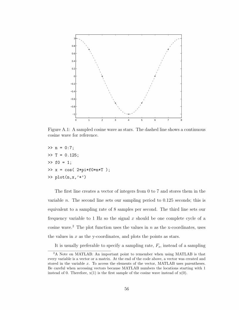
0 1 2 3 4 5 6 7 8
−1
−0.8
−0.6
−0.4
−0.2
0
0.2
0.4
0.6
0.8
1
Figure A.1: A sampled cosine wave as stars. The dashed line shows a continuouscosine wave for reference.
>> n = 0:7;
>> T = 0.125;
>> f0 = 1;
>> x = cos( 2*pi*f0*n*T );
>> plot(n,x,’*’)
The first line creates a vector of integers from 0 to 7 and stores them in the
variable n. The second line sets our sampling period to 0.125 seconds; this is
equivalent to a sampling rate of 8 samples per second. The third line sets our
frequency variable to 1 Hz so the signal x should be one complete cycle of a
cosine wave.2 The plot function uses the values in n as the x-coordinates, uses
the values in x as the y-coordinates, and plots the points as stars.
It is usually preferable to specify a sampling rate, Fs, instead of a sampling
2A Note on MATLAB: An important point to remember when using MATLAB is thatevery variable is a vector or a matrix. At the end of the code above, a vector was created andstored in the variable x. To access the elements of the vector, MATLAB uses parentheses.Be careful when accessing vectors because MATLAB numbers the locations starting with 1instead of 0. Therefore, x(1) is the first sample of the cosine wave instead of x(0).
56
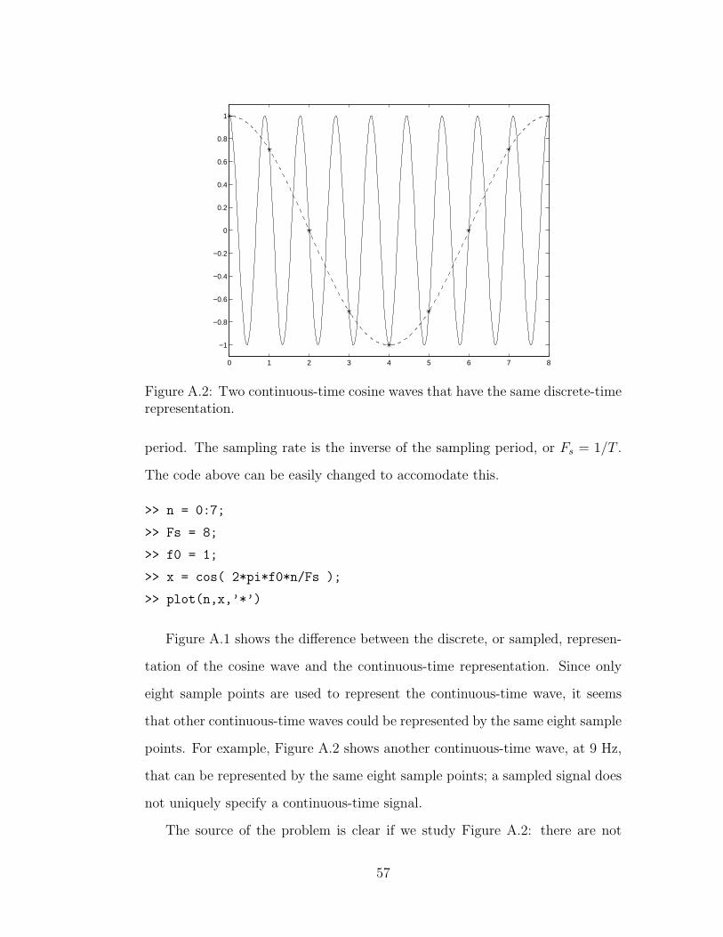
0 1 2 3 4 5 6 7 8
−1
−0.8
−0.6
−0.4
−0.2
0
0.2
0.4
0.6
0.8
1
Figure A.2: Two continuous-time cosine waves that have the same discrete-timerepresentation.
period. The sampling rate is the inverse of the sampling period, or Fs = 1/T .
The code above can be easily changed to accomodate this.
>> n = 0:7;
>> Fs = 8;
>> f0 = 1;
>> x = cos( 2*pi*f0*n/Fs );
>> plot(n,x,’*’)
Figure A.1 shows the difference between the discrete, or sampled, represen-
tation of the cosine wave and the continuous-time representation. Since only
eight sample points are used to represent the continuous-time wave, it seems
that other continuous-time waves could be represented by the same eight sample
points. For example, Figure A.2 shows another continuous-time wave, at 9 Hz,
that can be represented by the same eight sample points; a sampled signal does
not uniquely specify a continuous-time signal.
The source of the problem is clear if we study Figure A.2: there are not
57
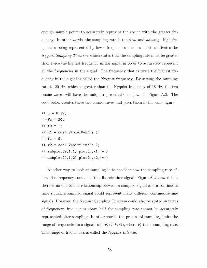
enough sample points to accurately represent the cosine with the greater fre-
quency. In other words, the sampling rate is too slow and aliasing—high fre-
quencies being represented by lower frequencies—occurs. This motivates the
Nyquist Sampling Theorem, which states that the sampling rate must be greater
than twice the highest frequency in the signal in order to accurately represent
all the frequencies in the signal. The frequency that is twice the highest fre-
quency in the signal is called the Nyquist frequency. By setting the sampling
rate to 20 Hz, which is greater than the Nyquist frequency of 18 Hz, the two
cosine waves will have the unique representations shown in Figure A.3. The
code below creates these two cosine waves and plots them in the same figure.
>> n = 0:19;
>> Fs = 20;
>> f0 = 1;
>> x1 = cos( 2*pi*f0*n/Fs );
>> f1 = 9;
>> x2 = cos( 2*pi*f1*n/Fs );
>> subplot(2,1,1),plot(n,x1,’*’)
>> subplot(2,1,2),plot(n,x2,’*’)
Another way to look at sampling is to consider how the sampling rate af-
fects the frequency content of the discrete-time signal. Figure A.2 showed that
there is no one-to-one relationship between a sampled signal and a continuous
time signal; a sampled signal could represent many different continuous-time
signals. However, the Nyquist Sampling Theorem could also be stated in terms
of frequency: frequencies above half the sampling rate cannot be accurately
represented after sampling. In other words, the process of sampling limits the
range of frequencies in a signal to [−Fs/2, Fs/2), where Fs is the sampling rate.
This range of frequencies is called the Nyquist Interval.
58
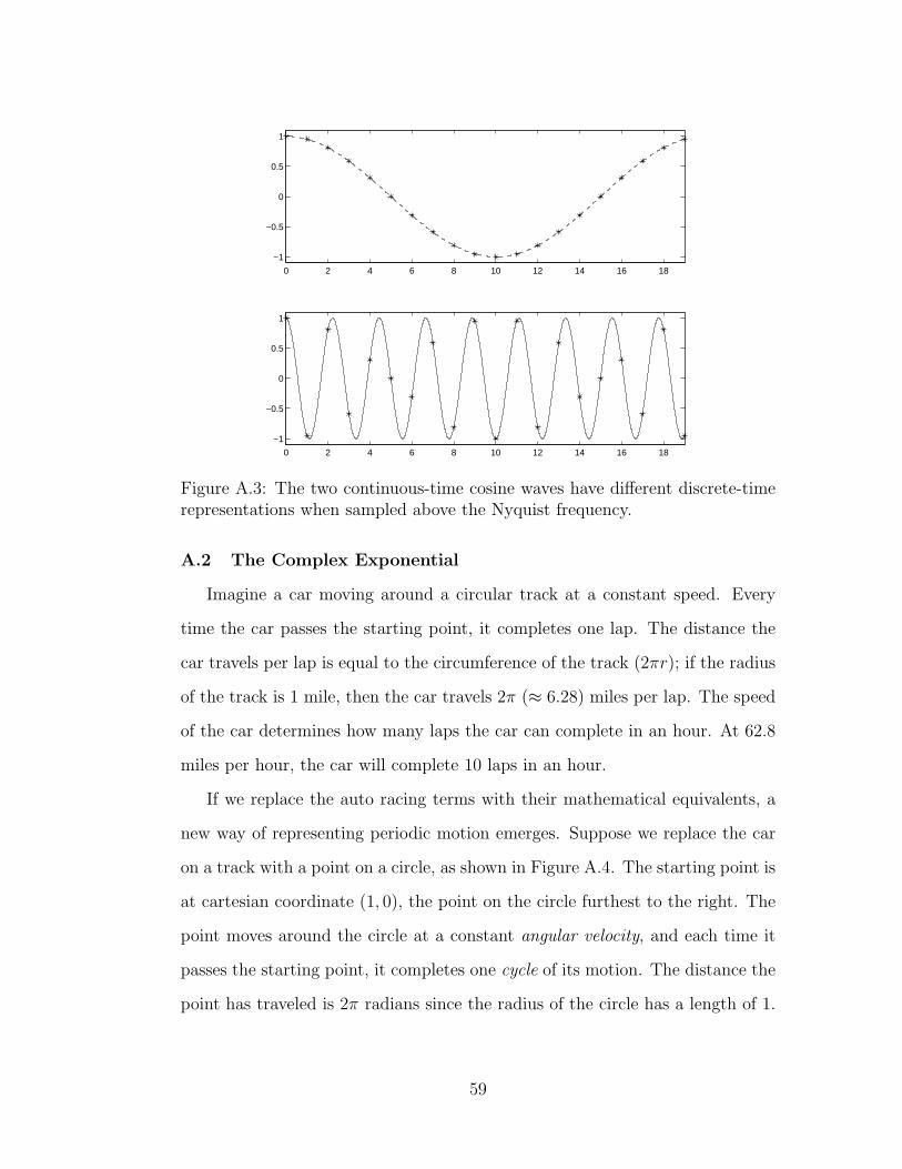
0 2 4 6 8 10 12 14 16 18
−1
−0.5
0
0.5
1
0 2 4 6 8 10 12 14 16 18
−1
−0.5
0
0.5
1
Figure A.3: The two continuous-time cosine waves have different discrete-timerepresentations when sampled above the Nyquist frequency.
A.2 The Complex Exponential
Imagine a car moving around a circular track at a constant speed. Every
time the car passes the starting point, it completes one lap. The distance the
car travels per lap is equal to the circumference of the track (2πr); if the radius
of the track is 1 mile, then the car travels 2π (≈ 6.28) miles per lap. The speed
of the car determines how many laps the car can complete in an hour. At 62.8
miles per hour, the car will complete 10 laps in an hour.
If we replace the auto racing terms with their mathematical equivalents, a
new way of representing periodic motion emerges. Suppose we replace the car
on a track with a point on a circle, as shown in Figure A.4. The starting point is
at cartesian coordinate (1, 0), the point on the circle furthest to the right. The
point moves around the circle at a constant angular velocity, and each time it
passes the starting point, it completes one cycle of its motion. The distance the
point has traveled is 2π radians since the radius of the circle has a length of 1.
59
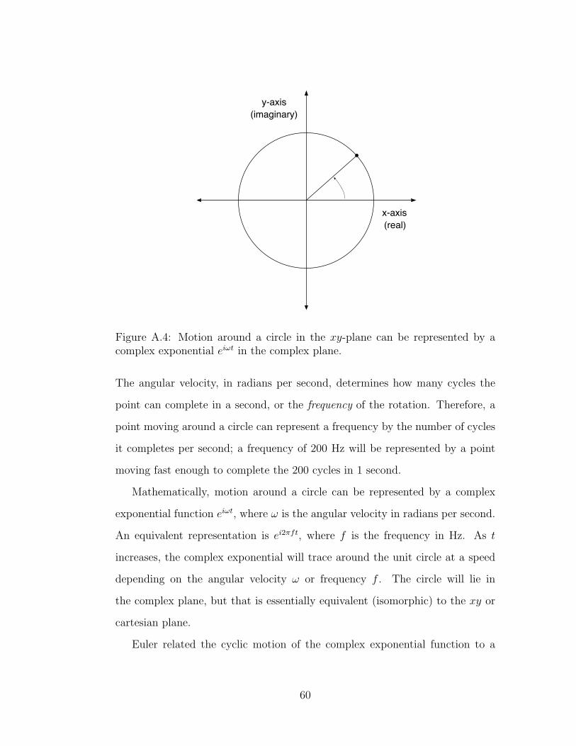
x-axis(real)
y-axis(imaginary)
Figure A.4: Motion around a circle in the xy-plane can be represented by acomplex exponential eiωt in the complex plane.
The angular velocity, in radians per second, determines how many cycles the
point can complete in a second, or the frequency of the rotation. Therefore, a
point moving around a circle can represent a frequency by the number of cycles
it completes per second; a frequency of 200 Hz will be represented by a point
moving fast enough to complete the 200 cycles in 1 second.
Mathematically, motion around a circle can be represented by a complex
exponential function eiωt, where ω is the angular velocity in radians per second.
An equivalent representation is ei2πft, where f is the frequency in Hz. As t
increases, the complex exponential will trace around the unit circle at a speed
depending on the angular velocity ω or frequency f . The circle will lie in
the complex plane, but that is essentially equivalent (isomorphic) to the xy or
cartesian plane.
Euler related the cyclic motion of the complex exponential function to a
60
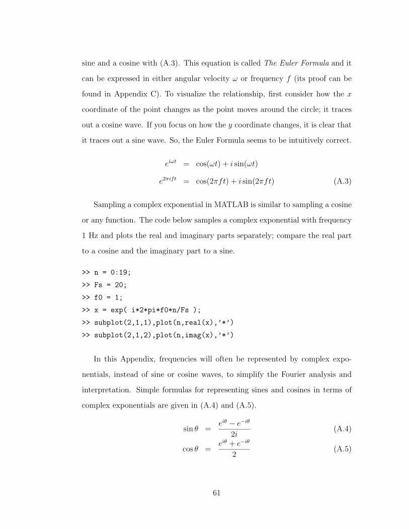
sine and a cosine with (A.3). This equation is called The Euler Formula and it
can be expressed in either angular velocity ω or frequency f (its proof can be
found in Appendix C). To visualize the relationship, first consider how the x
coordinate of the point changes as the point moves around the circle; it traces
out a cosine wave. If you focus on how the y coordinate changes, it is clear that
it traces out a sine wave. So, the Euler Formula seems to be intuitively correct.
eiωt = cos(ωt) + i sin(ωt)
e2πift = cos(2πft) + i sin(2πft) (A.3)
Sampling a complex exponential in MATLAB is similar to sampling a cosine
or any function. The code below samples a complex exponential with frequency
1 Hz and plots the real and imaginary parts separately; compare the real part
to a cosine and the imaginary part to a sine.
>> n = 0:19;
>> Fs = 20;
>> f0 = 1;
>> x = exp( i*2*pi*f0*n/Fs );
>> subplot(2,1,1),plot(n,real(x),’*’)
>> subplot(2,1,2),plot(n,imag(x),’*’)
In this Appendix, frequencies will often be represented by complex expo-
nentials, instead of sine or cosine waves, to simplify the Fourier analysis and
interpretation. Simple formulas for representing sines and cosines in terms of
complex exponentials are given in (A.4) and (A.5).
sin θ =eiθ − e−iθ
2i(A.4)
cos θ =eiθ + e−iθ
2(A.5)
61
A.3 Discrete Fourier Transform
The Fourier Transform shown (A.6) transforms a continuous-time function
x(t) into a continuous-frequency function X(ω). The same equation can also
be written in terms of frequency f instead of angular velocity ω; this version
is shown in (A.7). As mentioned above, a continuous-time function must be
sampled in order to be represented in the computer. By the same reasoning, a
continuous-frequency function must also be sampled in order to be represented
in the computer.
X(ω) =∫
x(t)e−iωtdt (A.6)
X(f) =∫
x(t)e−i2πftdt (A.7)
In (A.7), the complex exponential is a function of time t and frequency f .
To sample this function in time, replace t with nT , where T is the sampling
period and n is an integer. The sampled complex exponential is then e−i2πfnT .
To sample the frequency variable f , remember that sampling a signal in
the time domain restricts the possible frequencies to a range of [−Fs/2, Fs/2),
where Fs is the sampling rate. The continuous range of frequencies from −Fs/2
to Fs/2 can be pictured as a line from −Fs/2 to Fs/2. This is shown in the top
line of Figure A.5.
It is often more convenient to picture this range as positive frequencies from
0 to Fs. These two frequency ranges are equivalent when sampled at Fs be-
cause frequencies above Fs/2 will alias to negative frequencies. To sample the
frequency range from [0, Fs), let N be the number of frequency samples. Then
the sequence ak = kFs/N , will be N evenly spaced frequency samples between
0 and Fs. A sampled frequency range for N = 8 and Fs = 32 is shown in
Figure A.5.
62
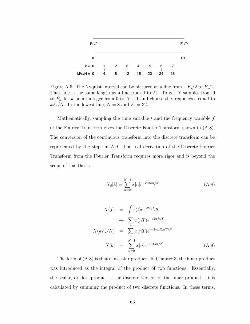
Fs/2-Fs/2
Fs0
0 1 2 3 4 5 6 7k =
kFs/N = 0 4 8 12 16 20 24 28
Figure A.5: The Nyquist Interval can be pictured as a line from −Fs/2 to Fs/2.That line is the same length as a line from 0 to Fs. To get N samples from 0to Fs, let k be an integer from 0 to N − 1 and choose the frequencies equal tokFs/N . In the lowest line, N = 8 and Fs = 32.
Mathematically, sampling the time variable t and the frequency variable f
of the Fourier Transform gives the Discrete Fourier Transform shown in (A.8).
The conversion of the continuous transform into the discrete transform can be
represented by the steps in A.9. The real derivation of the Discrete Fourier
Transform from the Fourier Transform requires more rigor and is beyond the
scope of this thesis.
Xd[k] =N−1∑n=0
x[n]e−i2πkn/N (A.8)
X(f) =∫
x(t)e−i2πftdt
→∑n
x(nT )e−i2πfnT
X(kFs/N) =∑n
x(nT )e−i2πkFsnT/N
X[k] =N−1∑n=0
x[n]e−i2πkn/N (A.9)
The form of (A.8) is that of a scalar product. In Chapter 3, the inner product
was introduced as the integral of the product of two functions. Essentially,
the scalar, or dot, product is the discrete version of the inner product. It is
calculated by summing the product of two discrete functions. In these terms,
63
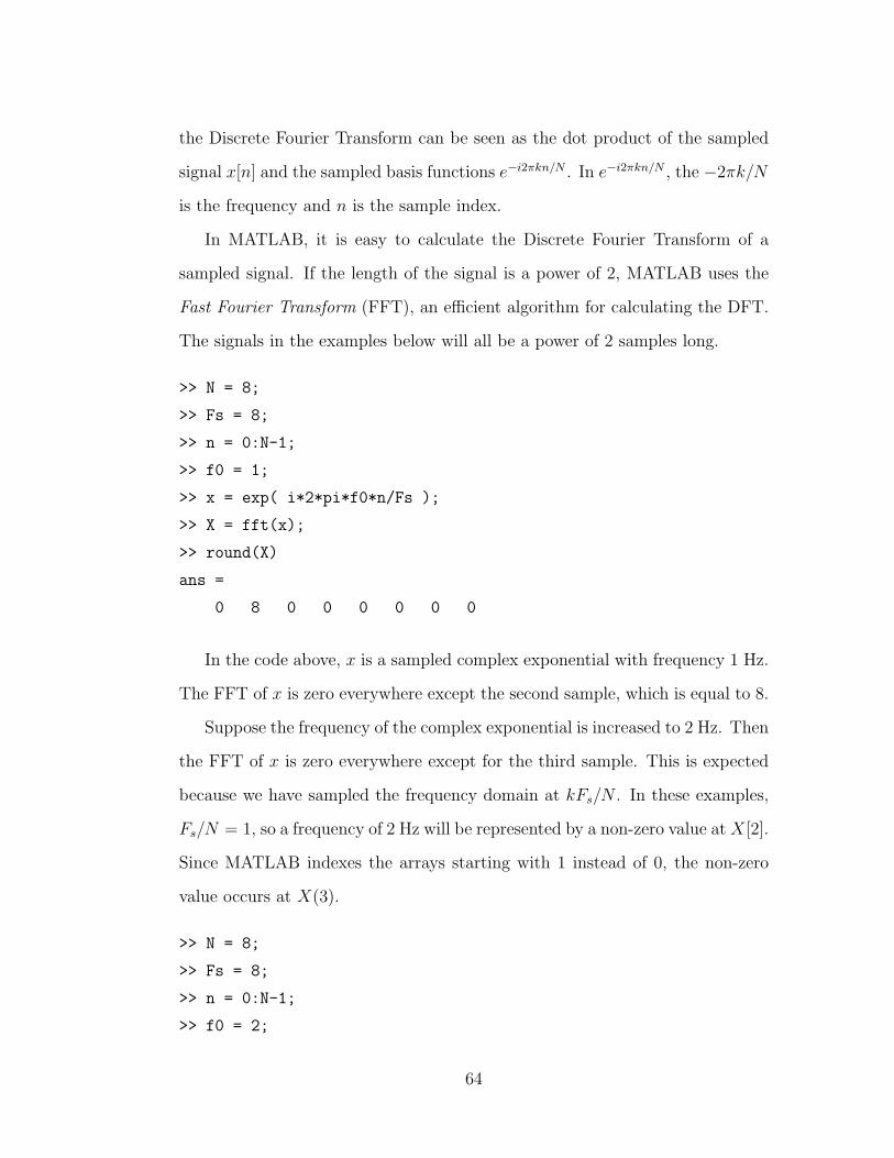
the Discrete Fourier Transform can be seen as the dot product of the sampled
signal x[n] and the sampled basis functions e−i2πkn/N . In e−i2πkn/N , the −2πk/N
is the frequency and n is the sample index.
In MATLAB, it is easy to calculate the Discrete Fourier Transform of a
sampled signal. If the length of the signal is a power of 2, MATLAB uses the
Fast Fourier Transform (FFT), an efficient algorithm for calculating the DFT.
The signals in the examples below will all be a power of 2 samples long.
>> N = 8;
>> Fs = 8;
>> n = 0:N-1;
>> f0 = 1;
>> x = exp( i*2*pi*f0*n/Fs );
>> X = fft(x);
>> round(X)
ans =
0 8 0 0 0 0 0 0
In the code above, x is a sampled complex exponential with frequency 1 Hz.
The FFT of x is zero everywhere except the second sample, which is equal to 8.
Suppose the frequency of the complex exponential is increased to 2 Hz. Then
the FFT of x is zero everywhere except for the third sample. This is expected
because we have sampled the frequency domain at kFs/N . In these examples,
Fs/N = 1, so a frequency of 2 Hz will be represented by a non-zero value at X[2].
Since MATLAB indexes the arrays starting with 1 instead of 0, the non-zero
value occurs at X(3).
>> N = 8;
>> Fs = 8;
>> n = 0:N-1;
>> f0 = 2;
64
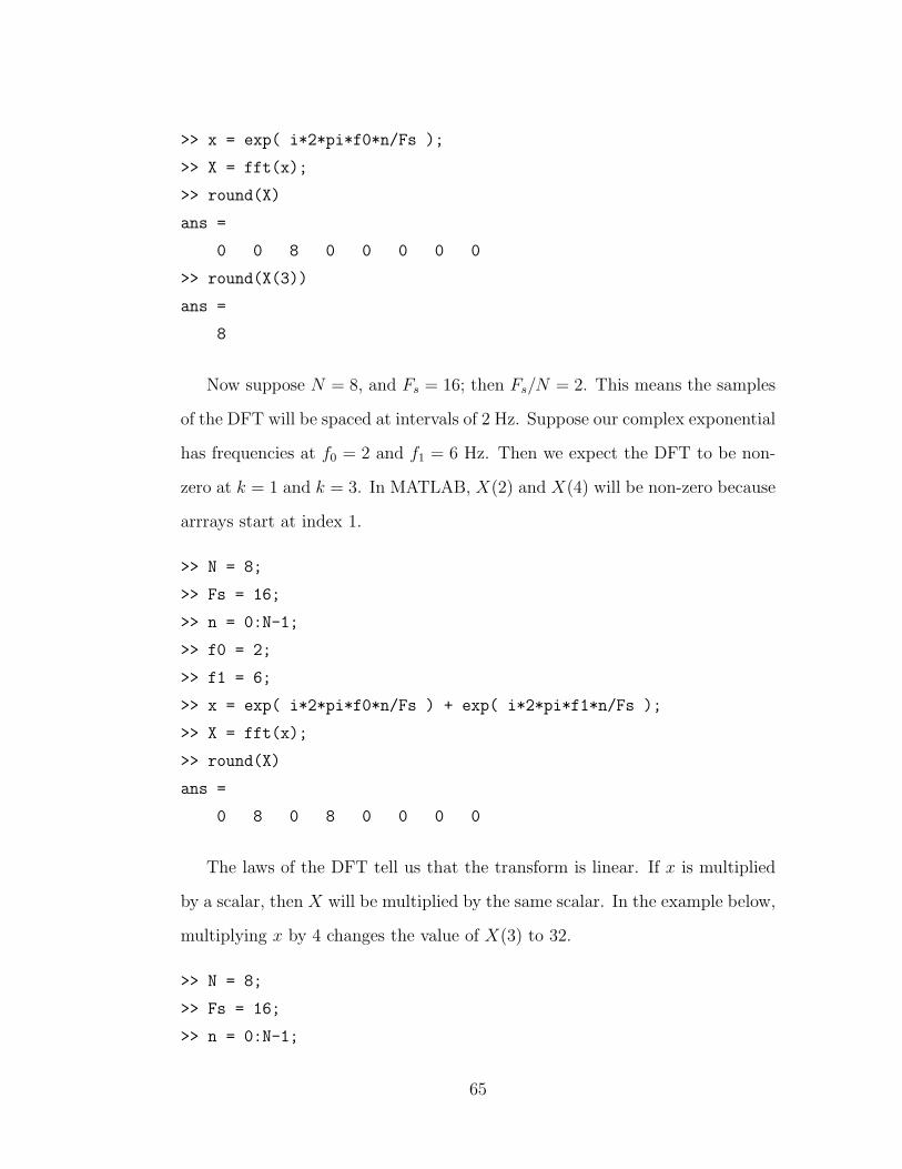
>> x = exp( i*2*pi*f0*n/Fs );
>> X = fft(x);
>> round(X)
ans =
0 0 8 0 0 0 0 0
>> round(X(3))
ans =
8
Now suppose N = 8, and Fs = 16; then Fs/N = 2. This means the samples
of the DFT will be spaced at intervals of 2 Hz. Suppose our complex exponential
has frequencies at f0 = 2 and f1 = 6 Hz. Then we expect the DFT to be non-
zero at k = 1 and k = 3. In MATLAB, X(2) and X(4) will be non-zero because
arrrays start at index 1.
>> N = 8;
>> Fs = 16;
>> n = 0:N-1;
>> f0 = 2;
>> f1 = 6;
>> x = exp( i*2*pi*f0*n/Fs ) + exp( i*2*pi*f1*n/Fs );
>> X = fft(x);
>> round(X)
ans =
0 8 0 8 0 0 0 0
The laws of the DFT tell us that the transform is linear. If x is multiplied
by a scalar, then X will be multiplied by the same scalar. In the example below,
multiplying x by 4 changes the value of X(3) to 32.
>> N = 8;
>> Fs = 16;
>> n = 0:N-1;
65
>> f0 = 4;
>> x = 4*exp( i*2*pi*f0*n/Fs );
>> X = fft(x);
>> round(X)
ans =
0 0 32 0 0 0 0 0
If we let N = 16 in the code above, then the frequency domain will be
sampled at intervals of Fs/N = 1 Hz again and the non-zero sample will be
found at X(5) in MATLAB. The value at X(5) has changed because of the
change of N , the DFT size. This motivates normalization of the DFT by the
DFT size (Appendix B will show that the normalization should use the window
size when it is different from the DFT size).
>> N = 16;
>> Fs = 16;
>> n = 0:N-1;
>> f0 = 4;
>> x = 4*exp( i*2*pi*f0*n/Fs );
>> X = fft(x);
>> round(X)
ans =
0 0 0 0 64 0 0 0 0 0 0 0 0 0 0 0
>> round(X)/N
ans =
0 0 0 0 4 0 0 0 0 0 0 0 0 0 0 0
So far, we have seen that the frequency range of the DFT is sampled at intervals
of Fs/N and that if the frequency of a complex exponential is an exact multiple
of Fs/N , then the DFT will be zero everywhere except at one sample. The value
of this sample will be the amplitude of the complex exponential multiplied by
the DFT size. This is why it is common practice to normalize by the DFT size.
66
There are several basic concepts still left to cover. The first is that the
values of the DFT are actually complex (a± bi). In the examples above, the b
term was equal to zero and the round function was used to simplify the output.
Typically, the b term is not zero and the complex values are converted into polar
coordinates, or magnitude and phase. The MATLAB functions that convert a
complex number to magnitude and phase are abs and angle.
>> N = 8;
>> Fs = 8;
>> n = 0:N-1;
>> f0 = 2;
>> x = 2*exp( i*2*pi*f0*n/Fs );
>> X = fft(x);
>> mag = abs(X)/N;
>> phs = angle(X);
>> mag
mag =
0 0 2 0 0 0 0 0
>> phs
phs =
2.36 2.75 -0.00 0.39 0.79 1.18 1.57 1.96
In the code above, all of the phase values except phs(3) should be ignored
since the corresponding magnitude values are zero. Analyzing the phase will be
discussed in Appendix B. Next, I will show what happens when the input signal
is a sine wave or a cosine wave instead of a complex exponential.
>> N = 8;
>> Fs = 8;
>> n = 0:N-1;
>> f0 = 2;
>> sn = 2*sin( 2*pi*f0*n/Fs );
>> SN = fft(sn);
67
>> mag_sn = abs(SN)/N;
>> phs_sn = angle(SN);
>> mag_sn
mag_sn =
0 0 1 0 0 0 1 0
>> phs_sn
phs_sn =
0.00 0.78 -1.57 -0.79 0.00 0.79 1.57 -0.79
>> cs = 2*cos( 2*pi*f0*n/Fs );
>> CS = fft(cs);
>> mag_cs = abs(CS)/N;
>> phs_cs = angle(CS);
>> mag_cs
mag_cs =
0 0 1 0 0 0 1 0
>> phs_cs
phs_cs =
0.39 0.39 -0.00 0.00 0.00 -0.00 0.00 -0.39
When the signal is real, two samples of the DFT are non-zero: one for f0 and
the other for −f0. Equations A.4 and A.5 show why this happens; a sine or
cosine wave can be expressed as a sum of complex exponentials. These two
signals are shown in Figure A.6. When analyzing real signals it is common to
only view half of the frequency samples since the other half will have exactly
the same information.
Suppose the frequency of the input signal is not an exact multiple of Fs/N .
The DFT capable of representing any frequency between [−Fs/2, Fs/2). The
code below creates a sine wave with a frequency of 2.2 Hz. Comparing Figure A.7
to Figure A.6(a) shows that the peaks at SN(2) and SN(6) are still present but
Figure A.7 also has energy at other samples. The spread of energy to frequency
samples far from the peak is termed spectral leakage.
68
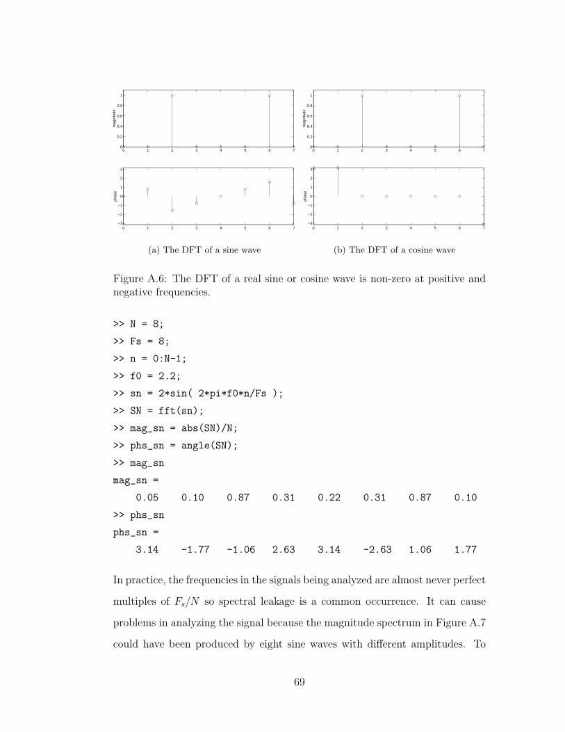
0 1 2 3 4 5 6 70
0.2
0.4
0.6
0.8
1
mag
nitu
de
0 1 2 3 4 5 6 7−3
−2
−1
0
1
2
3
phas
e
(a) The DFT of a sine wave
0 1 2 3 4 5 6 70
0.2
0.4
0.6
0.8
1
mag
nitu
de
0 1 2 3 4 5 6 7−3
−2
−1
0
1
2
3
phas
e
(b) The DFT of a cosine wave
Figure A.6: The DFT of a real sine or cosine wave is non-zero at positive andnegative frequencies.
>> N = 8;
>> Fs = 8;
>> n = 0:N-1;
>> f0 = 2.2;
>> sn = 2*sin( 2*pi*f0*n/Fs );
>> SN = fft(sn);
>> mag_sn = abs(SN)/N;
>> phs_sn = angle(SN);
>> mag_sn
mag_sn =
0.05 0.10 0.87 0.31 0.22 0.31 0.87 0.10
>> phs_sn
phs_sn =
3.14 -1.77 -1.06 2.63 3.14 -2.63 1.06 1.77
In practice, the frequencies in the signals being analyzed are almost never perfect
multiples of Fs/N so spectral leakage is a common occurrence. It can cause
problems in analyzing the signal because the magnitude spectrum in Figure A.7
could have been produced by eight sine waves with different amplitudes. To
69
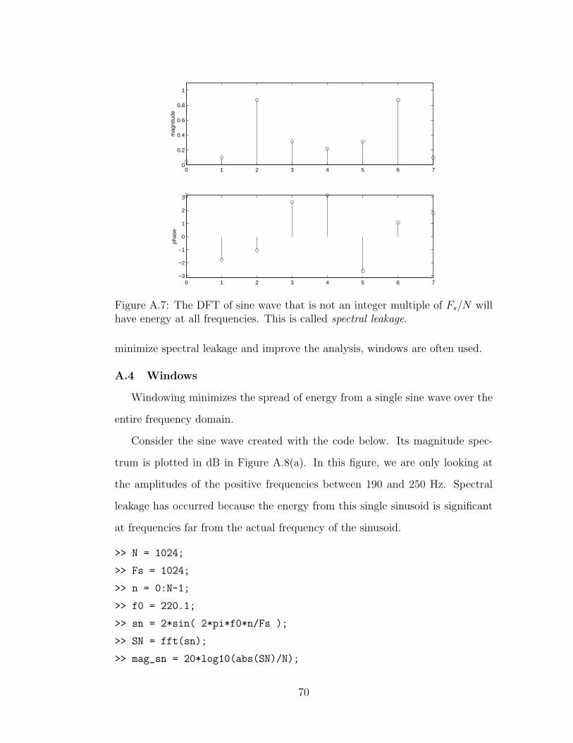
0 1 2 3 4 5 6 70
0.2
0.4
0.6
0.8
1
mag
nitu
de
0 1 2 3 4 5 6 7−3
−2
−1
0
1
2
3
phas
e
Figure A.7: The DFT of sine wave that is not an integer multiple of Fs/N willhave energy at all frequencies. This is called spectral leakage.
minimize spectral leakage and improve the analysis, windows are often used.
A.4 Windows
Windowing minimizes the spread of energy from a single sine wave over the
entire frequency domain.
Consider the sine wave created with the code below. Its magnitude spec-
trum is plotted in dB in Figure A.8(a). In this figure, we are only looking at
the amplitudes of the positive frequencies between 190 and 250 Hz. Spectral
leakage has occurred because the energy from this single sinusoid is significant
at frequencies far from the actual frequency of the sinusoid.
>> N = 1024;
>> Fs = 1024;
>> n = 0:N-1;
>> f0 = 220.1;
>> sn = 2*sin( 2*pi*f0*n/Fs );
>> SN = fft(sn);
>> mag_sn = 20*log10(abs(SN)/N);
70
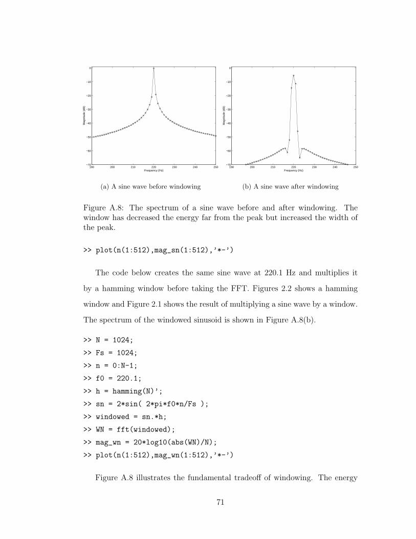
190 200 210 220 230 240 250−70
−60
−50
−40
−30
−20
−10
0
Frequency (Hz)
Mag
nitu
de (
dB)
(a) A sine wave before windowing
190 200 210 220 230 240 250−70
−60
−50
−40
−30
−20
−10
0
Frequency (Hz)
Mag
nitu
de (
dB)
(b) A sine wave after windowing
Figure A.8: The spectrum of a sine wave before and after windowing. Thewindow has decreased the energy far from the peak but increased the width ofthe peak.
>> plot(n(1:512),mag_sn(1:512),’*-’)
The code below creates the same sine wave at 220.1 Hz and multiplies it
by a hamming window before taking the FFT. Figures 2.2 shows a hamming
window and Figure 2.1 shows the result of multiplying a sine wave by a window.
The spectrum of the windowed sinusoid is shown in Figure A.8(b).
>> N = 1024;
>> Fs = 1024;
>> n = 0:N-1;
>> f0 = 220.1;
>> h = hamming(N)’;
>> sn = 2*sin( 2*pi*f0*n/Fs );
>> windowed = sn.*h;
>> WN = fft(windowed);
>> mag_wn = 20*log10(abs(WN)/N);
>> plot(n(1:512),mag_wn(1:512),’*-’)
Figure A.8 illustrates the fundamental tradeoff of windowing. The energy
71

far from the peak has been decreased by the window, minimizing the effects of
spectral leakage. The cost of windowing is an increased main lobe width, which
can make close frequencies difficult to detect.
72

B Beyond the Basics
This appendix covers techniques for extracting accurate frequency, amplitude,
and phase values from the DFT in MATLAB.
B.1 Parabolic Interpolation
Consider the sampled sinusoid created with the code below. It is 2048 points
of a 220 Hz sine wave at a sampling rate of 44100 Hz. The plot command plots
the magnitude spectrum, shown in Figure B.1. The axis command scales the
plot to show frequency samples 7 to 16 and amplitude values 0 to 0.6.
>> Fs = 44100;
>> N = 2048;
>> n = 0:N-1;
>> f0 = 220;
>> h = hamming(N)’;
>> sn = 2*sin( 2*pi*f0*n/Fs ).*h;
>> mag_sn = abs(fft(sn))/N;
>> plot(mag_sn(1:N/2),’*-’)
>> axis([7 16 0 0.6])
The highest point in Figure B.1 occurs at frequency sample 11. Appendix A
showed that the frequency domain of the DFT is sampled at intervals of Fs/N .
In this case, every frequency bin is Fs/N = 44100/2048 = 21.5332 Hz apart,
so the frequency in Hz at bin 11 is 10 ∗ 21.5332 = 215.332 Hz (remember that
MATLAB numbers arrays starting at index 1). This value can also be found
using the max command, which returns the maximum value in an array and its
index.
>> [v,ix] = max(mag_sn);
v =
0.5198
73
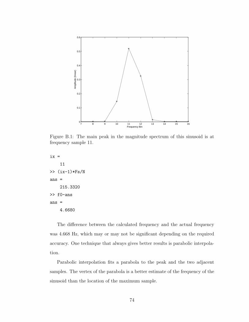
7 8 9 10 11 12 13 14 15 160
0.1
0.2
0.3
0.4
0.5
0.6
Frequency Bin
Am
plitu
de (
linea
r)
Figure B.1: The main peak in the magnitude spectrum of this sinusoid is atfrequency sample 11.
ix =
11
>> (ix-1)*Fs/N
ans =
215.3320
>> f0-ans
ans =
4.6680
The difference between the calculated frequency and the actual frequency
was 4.668 Hz, which may or may not be significant depending on the required
accuracy. One technique that always gives better results is parabolic interpola-
tion.
Parabolic interpolation fits a parabola to the peak and the two adjacent
samples. The vertex of the parabola is a better estimate of the frequency of the
sinusoid than the location of the maximum sample.
74
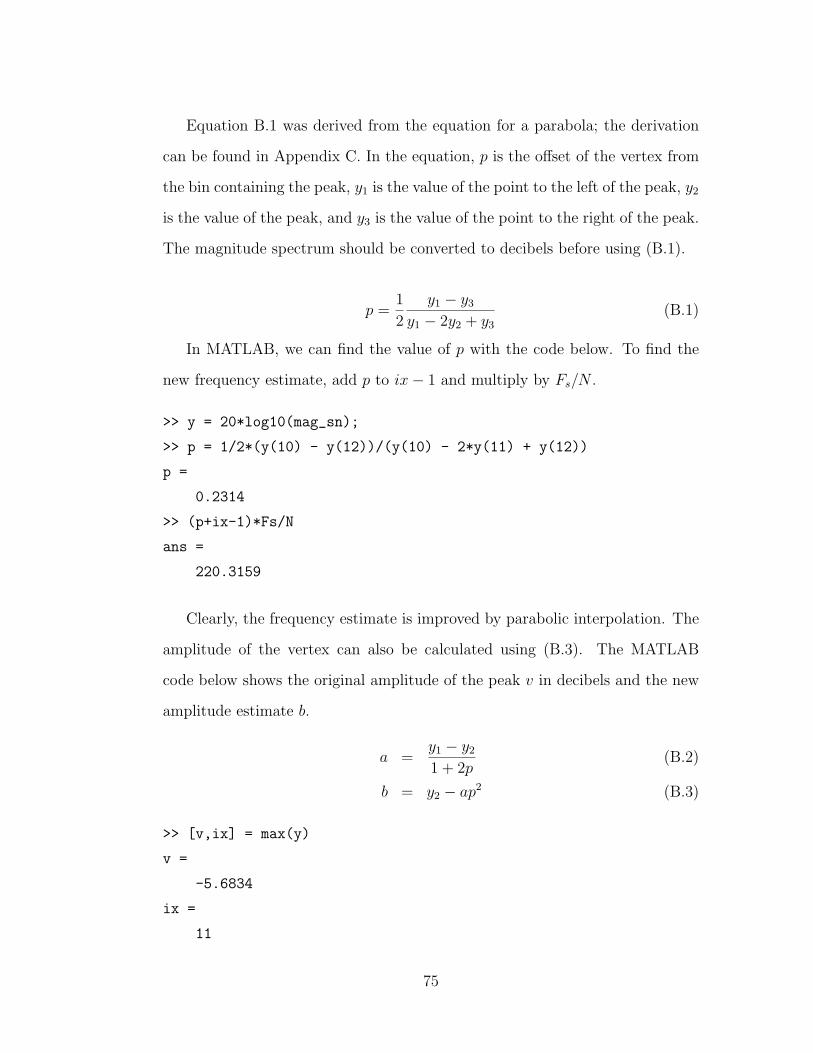
Equation B.1 was derived from the equation for a parabola; the derivation
can be found in Appendix C. In the equation, p is the offset of the vertex from
the bin containing the peak, y1 is the value of the point to the left of the peak, y2
is the value of the peak, and y3 is the value of the point to the right of the peak.
The magnitude spectrum should be converted to decibels before using (B.1).
p =1
2
y1 − y3
y1 − 2y2 + y3
(B.1)
In MATLAB, we can find the value of p with the code below. To find the
new frequency estimate, add p to ix− 1 and multiply by Fs/N .
>> y = 20*log10(mag_sn);
>> p = 1/2*(y(10) - y(12))/(y(10) - 2*y(11) + y(12))
p =
0.2314
>> (p+ix-1)*Fs/N
ans =
220.3159
Clearly, the frequency estimate is improved by parabolic interpolation. The
amplitude of the vertex can also be calculated using (B.3). The MATLAB
code below shows the original amplitude of the peak v in decibels and the new
amplitude estimate b.
a =y1 − y2
1 + 2p(B.2)
b = y2 − ap2 (B.3)
>> [v,ix] = max(y)
v =
-5.6834
ix =
11
75
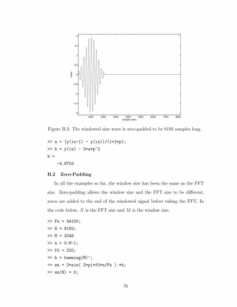
1000 2000 3000 4000 5000 6000 7000 8000
−2
−1.5
−1
−0.5
0
0.5
1
1.5
2
Sample Index
Val
ue
Figure B.2: The windowed sine wave is zero-padded to be 8192 samples long.
>> a = (y(ix-1) - y(ix))/(1+2*p);
>> b = y(ix) - 2*a*p^2
b =
-4.8703
B.2 Zero-Padding
In all the examples so far, the window size has been the same as the FFT
size. Zero-padding allows the window size and the FFT size to be different;
zeros are added to the end of the windowed signal before taking the FFT. In
the code below, N is the FFT size and M is the window size.
>> Fs = 44100;
>> N = 8192;
>> M = 2048
>> n = 0:M-1;
>> f0 = 220;
>> h = hamming(M)’;
>> sn = 2*sin( 2*pi*f0*n/Fs ).*h;
>> sn(N) = 0;
76
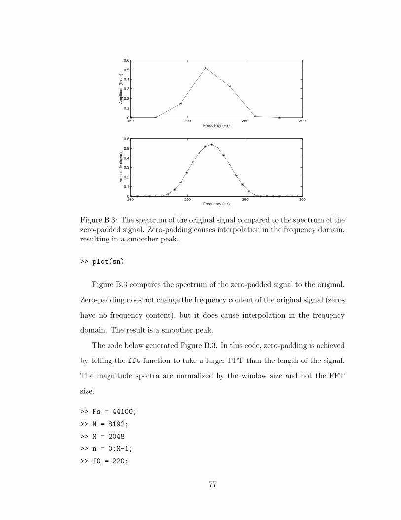
150 200 250 3000
0.1
0.2
0.3
0.4
0.5
0.6
Frequency (Hz)A
mpl
itude
(lin
ear)
150 200 250 3000
0.1
0.2
0.3
0.4
0.5
0.6
Frequency (Hz)
Am
plitu
de (
linea
r)
Figure B.3: The spectrum of the original signal compared to the spectrum of thezero-padded signal. Zero-padding causes interpolation in the frequency domain,resulting in a smoother peak.
>> plot(sn)
Figure B.3 compares the spectrum of the zero-padded signal to the original.
Zero-padding does not change the frequency content of the original signal (zeros
have no frequency content), but it does cause interpolation in the frequency
domain. The result is a smoother peak.
The code below generated Figure B.3. In this code, zero-padding is achieved
by telling the fft function to take a larger FFT than the length of the signal.
The magnitude spectra are normalized by the window size and not the FFT
size.
>> Fs = 44100;
>> N = 8192;
>> M = 2048
>> n = 0:M-1;
>> f0 = 220;
77
25 30 35 40 45 50 55 600
0.1
0.2
0.3
0.4
0.5
0.6
Sample IndexA
mpl
itude
(lin
ear)
25 30 35 40 45 50 55 60−6
−4
−2
0
2
4
6
Sample Index
Pha
se (
radi
ans)
Figure B.4: The phase values under the peak lie on a line with constant slope.
>> h = hamming(M)’;
>> sn = 2*sin( 2*pi*f0*n/Fs ).*h;
>> mag_sn = abs(fft(sn,M))/M;
>> mag_zero = abs(fft(sn,N))/M;
>> freq_sn = [0:M/2-1]’*Fs/M;
>> freq_zero = [0:N/2-1]’*Fs/N;
>> subplot(2,1,1),plot(freq_sn,mag_sn(1:M/2),’*-’)
>> axis([150 300 0 0.6])
>> subplot(2,1,2),plot(freq_zero,mag_zero(1:N/2),’*-’)
>> axis([150 300 0 0.6])
B.3 Centering the FFT Buffer for Phase Estimation
Consider the phase spectrum of cosine wave created by the code below and
shown in Figure B.4. The phase values under the peak lie on a sloped line. This
makes analysis difficult because it is not clear which of the values to use or if
the slope of the line is important.
>> Fs = 44100;
78
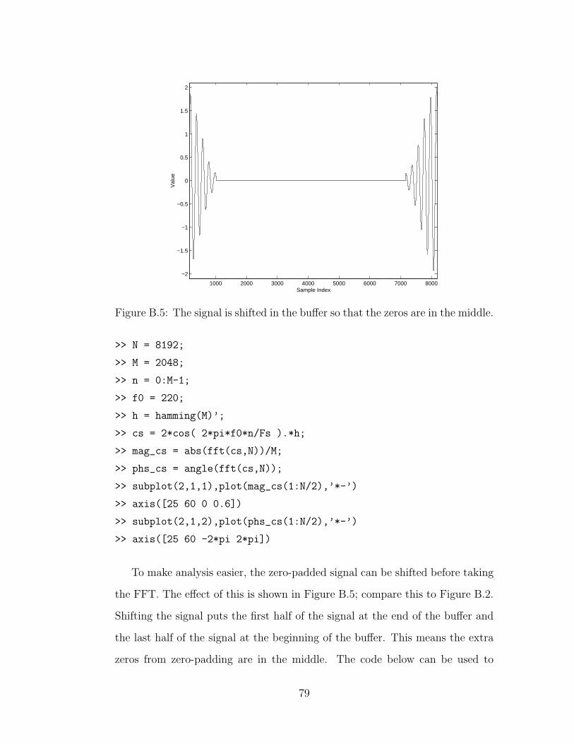
1000 2000 3000 4000 5000 6000 7000 8000
−2
−1.5
−1
−0.5
0
0.5
1
1.5
2
Sample Index
Val
ue
Figure B.5: The signal is shifted in the buffer so that the zeros are in the middle.
>> N = 8192;
>> M = 2048;
>> n = 0:M-1;
>> f0 = 220;
>> h = hamming(M)’;
>> cs = 2*cos( 2*pi*f0*n/Fs ).*h;
>> mag_cs = abs(fft(cs,N))/M;
>> phs_cs = angle(fft(cs,N));
>> subplot(2,1,1),plot(mag_cs(1:N/2),’*-’)
>> axis([25 60 0 0.6])
>> subplot(2,1,2),plot(phs_cs(1:N/2),’*-’)
>> axis([25 60 -2*pi 2*pi])
To make analysis easier, the zero-padded signal can be shifted before taking
the FFT. The effect of this is shown in Figure B.5; compare this to Figure B.2.
Shifting the signal puts the first half of the signal at the end of the buffer and
the last half of the signal at the beginning of the buffer. This means the extra
zeros from zero-padding are in the middle. The code below can be used to
79
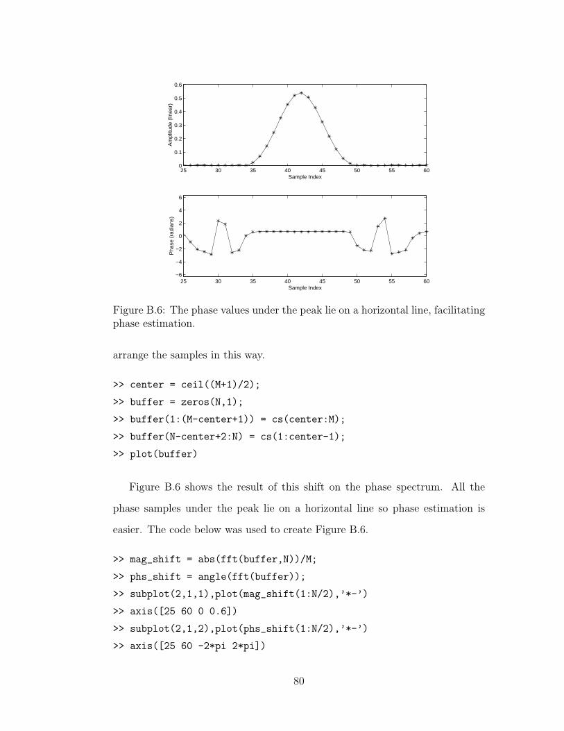
25 30 35 40 45 50 55 600
0.1
0.2
0.3
0.4
0.5
0.6
Sample IndexA
mpl
itude
(lin
ear)
25 30 35 40 45 50 55 60−6
−4
−2
0
2
4
6
Sample Index
Pha
se (
radi
ans)
Figure B.6: The phase values under the peak lie on a horizontal line, facilitatingphase estimation.
arrange the samples in this way.
>> center = ceil((M+1)/2);
>> buffer = zeros(N,1);
>> buffer(1:(M-center+1)) = cs(center:M);
>> buffer(N-center+2:N) = cs(1:center-1);
>> plot(buffer)
Figure B.6 shows the result of this shift on the phase spectrum. All the
phase samples under the peak lie on a horizontal line so phase estimation is
easier. The code below was used to create Figure B.6.
>> mag_shift = abs(fft(buffer,N))/M;
>> phs_shift = angle(fft(buffer));
>> subplot(2,1,1),plot(mag_shift(1:N/2),’*-’)
>> axis([25 60 0 0.6])
>> subplot(2,1,2),plot(phs_shift(1:N/2),’*-’)
>> axis([25 60 -2*pi 2*pi])
80
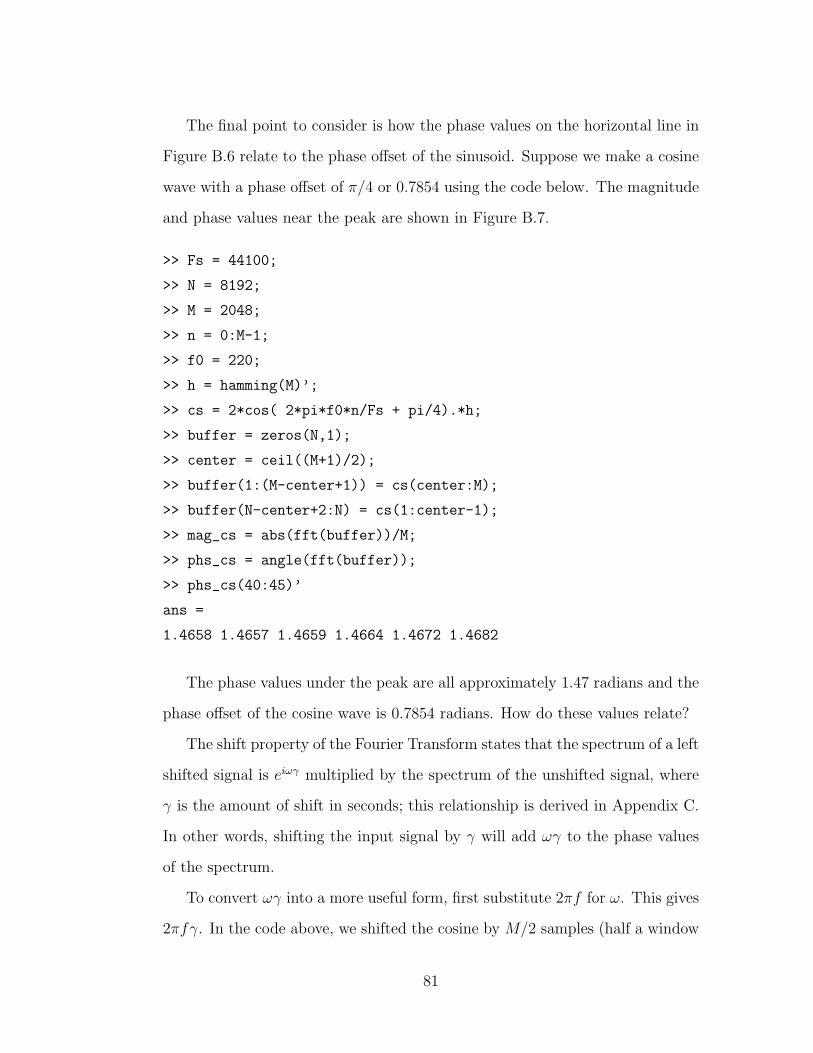
The final point to consider is how the phase values on the horizontal line in
Figure B.6 relate to the phase offset of the sinusoid. Suppose we make a cosine
wave with a phase offset of π/4 or 0.7854 using the code below. The magnitude
and phase values near the peak are shown in Figure B.7.
>> Fs = 44100;
>> N = 8192;
>> M = 2048;
>> n = 0:M-1;
>> f0 = 220;
>> h = hamming(M)’;
>> cs = 2*cos( 2*pi*f0*n/Fs + pi/4).*h;
>> buffer = zeros(N,1);
>> center = ceil((M+1)/2);
>> buffer(1:(M-center+1)) = cs(center:M);
>> buffer(N-center+2:N) = cs(1:center-1);
>> mag_cs = abs(fft(buffer))/M;
>> phs_cs = angle(fft(buffer));
>> phs_cs(40:45)’
ans =
1.4658 1.4657 1.4659 1.4664 1.4672 1.4682
The phase values under the peak are all approximately 1.47 radians and the
phase offset of the cosine wave is 0.7854 radians. How do these values relate?
The shift property of the Fourier Transform states that the spectrum of a left
shifted signal is eiωγ multiplied by the spectrum of the unshifted signal, where
γ is the amount of shift in seconds; this relationship is derived in Appendix C.
In other words, shifting the input signal by γ will add ωγ to the phase values
of the spectrum.
To convert ωγ into a more useful form, first substitute 2πf for ω. This gives
2πfγ. In the code above, we shifted the cosine by M/2 samples (half a window
81
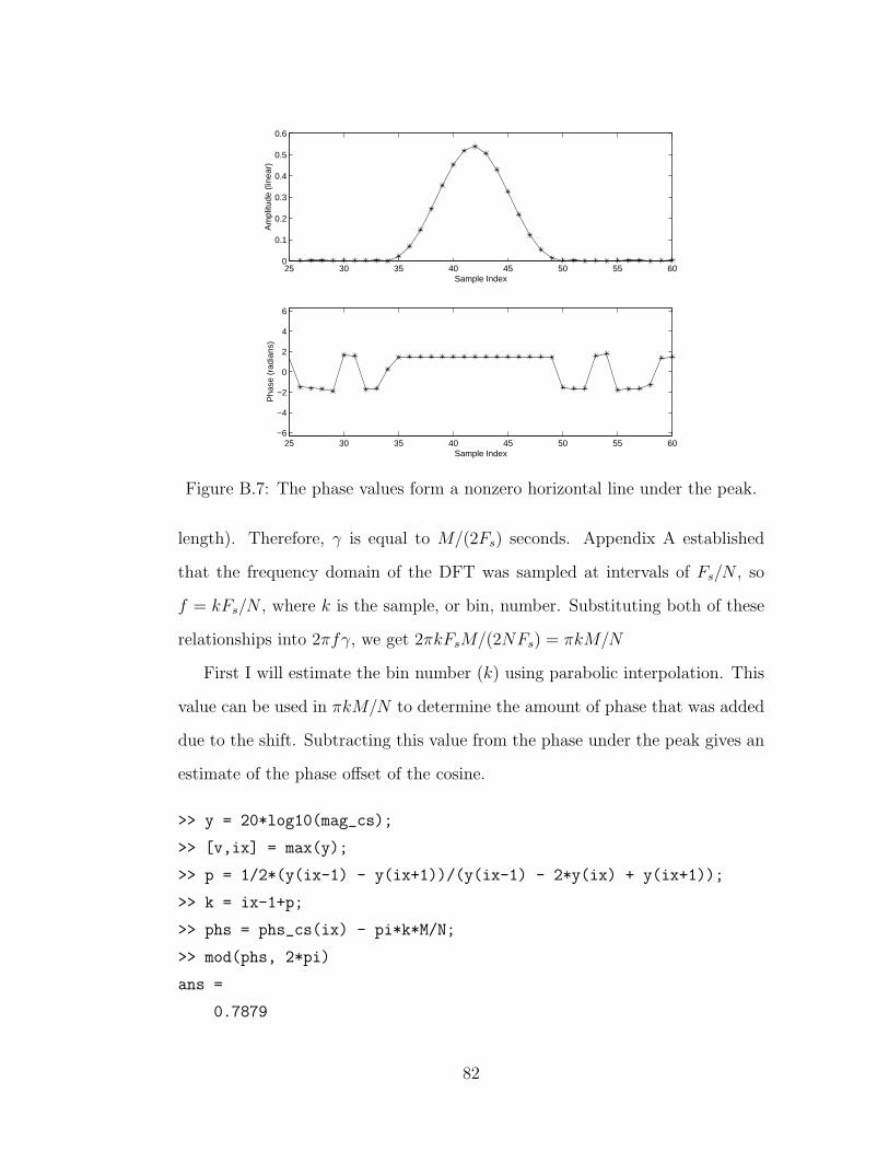
25 30 35 40 45 50 55 600
0.1
0.2
0.3
0.4
0.5
0.6
Sample IndexA
mpl
itude
(lin
ear)
25 30 35 40 45 50 55 60−6
−4
−2
0
2
4
6
Sample Index
Pha
se (
radi
ans)
Figure B.7: The phase values form a nonzero horizontal line under the peak.
length). Therefore, γ is equal to M/(2Fs) seconds. Appendix A established
that the frequency domain of the DFT was sampled at intervals of Fs/N , so
f = kFs/N , where k is the sample, or bin, number. Substituting both of these
relationships into 2πfγ, we get 2πkFsM/(2NFs) = πkM/N
First I will estimate the bin number (k) using parabolic interpolation. This
value can be used in πkM/N to determine the amount of phase that was added
due to the shift. Subtracting this value from the phase under the peak gives an
estimate of the phase offset of the cosine.
>> y = 20*log10(mag_cs);
>> [v,ix] = max(y);
>> p = 1/2*(y(ix-1) - y(ix+1))/(y(ix-1) - 2*y(ix) + y(ix+1));
>> k = ix-1+p;
>> phs = phs_cs(ix) - pi*k*M/N;
>> mod(phs, 2*pi)
ans =
0.7879
82
>> pi/4
ans =
0.7854
This Appendix has shown techniques for extracting accurate frequency, am-
plitude, and phase values from the Discrete Fourier Transform of a signal.
83
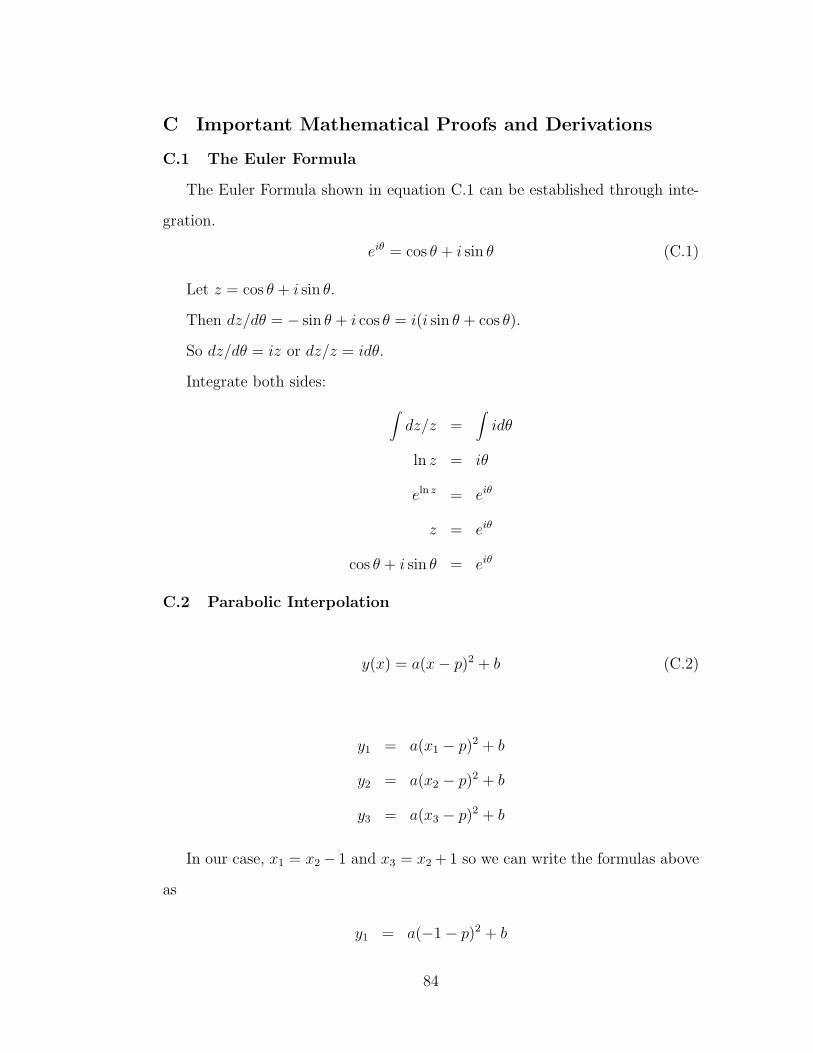
C Important Mathematical Proofs and Derivations
C.1 The Euler Formula
The Euler Formula shown in equation C.1 can be established through inte-
gration.
eiθ = cos θ + i sin θ (C.1)
Let z = cos θ + i sin θ.
Then dz/dθ = − sin θ + i cos θ = i(i sin θ + cos θ).
So dz/dθ = iz or dz/z = idθ.
Integrate both sides:
∫dz/z =
∫idθ
ln z = iθ
eln z = eiθ
z = eiθ
cos θ + i sin θ = eiθ
C.2 Parabolic Interpolation
y(x) = a(x− p)2 + b (C.2)
y1 = a(x1 − p)2 + b
y2 = a(x2 − p)2 + b
y3 = a(x3 − p)2 + b
In our case, x1 = x2− 1 and x3 = x2 + 1 so we can write the formulas above
as
y1 = a(−1− p)2 + b
84
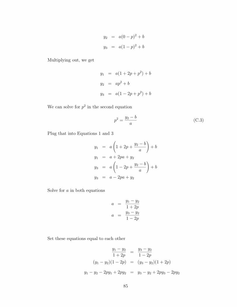
y2 = a(0− p)2 + b
y3 = a(1− p)2 + b
Multiplying out, we get
y1 = a(1 + 2p + p2) + b
y2 = ap2 + b
y3 = a(1− 2p + p2) + b
We can solve for p2 in the second equation
p2 =y2 − b
a(C.3)
Plug that into Equations 1 and 3
y1 = a
(1 + 2p +
y2 − b
a
)+ b
y1 = a + 2pa + y2
y3 = a
(1− 2p +
y2 − b
a
)+ b
y3 = a− 2pa + y2
Solve for a in both equations
a =y1 − y2
1 + 2p
a =y3 − y2
1− 2p
Set these equations equal to each other
y1 − y2
1 + 2p=
y3 − y2
1− 2p
(y1 − y2)(1− 2p) = (y3 − y2)(1 + 2p)
y1 − y2 − 2py1 + 2py2 = y3 − y2 + 2py3 − 2py2
85
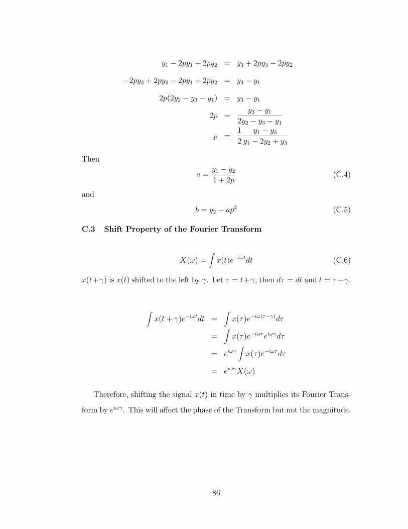
y1 − 2py1 + 2py2 = y3 + 2py3 − 2py2
−2py3 + 2py2 − 2py1 + 2py2 = y3 − y1
2p(2y2 − y3 − y1) = y3 − y1
2p =y3 − y1
2y2 − y3 − y1
p =1
2
y1 − y3
y1 − 2y2 + y3
Then
a =y1 − y2
1 + 2p(C.4)
and
b = y2 − ap2 (C.5)
C.3 Shift Property of the Fourier Transform
X(ω) =∫
x(t)e−iωtdt (C.6)
x(t+γ) is x(t) shifted to the left by γ. Let τ = t+γ, then dτ = dt and t = τ−γ.
∫x(t + γ)e−iωtdt =
∫x(τ)e−iω(τ−γ)dτ
=∫
x(τ)e−iωτeiωγdτ
= eiωγ∫
x(τ)e−iωτdτ
= eiωγX(ω)
Therefore, shifting the signal x(t) in time by γ multiplies its Fourier Trans-
form by eiωγ. This will affect the phase of the Transform but not the magnitude.
86
Bibliography
Akay, M. and Mello, C., “Time-Frequency and Time-Scale (Wavelets) Analysis
Methods: Design and Algorithms,” Smart Engineering System Design, vol. 1,
pp. 77–94, 1998.
Auger, F., Flandrin, P., Lemoine, O., and Goncalves, P., “Time-Frequency Tool-
box for MATLAB,” http://crttsn.univ-nantes.fr/~auger/tftb.html,
1999.
Bregman, A. S., Auditory Scene Analysis. Cambridge, MA: The MIT Press,
second ed., 1990.
Chen, C.-T., Digital Signal Processing. New York: Oxford University Press,
Inc., first ed., 2001.
Daubechies, I., Ten Lectures on Wavelets. Philadelphia: Society for Industrial
and Applied Mathematics, first ed., 1992.
Dolson, M., “The Phase Vocoder: A Tutorial,” Computer Music Journal,
vol. 10, pp. 14–28, 1986.
Gabor, D., “Theory of Communication,” Journal of the IEEE, vol. 93, pp. 429–
457, 1946.
Gelfand, S. A., Hearing. New York: Marcel Dekker, Inc., third ed., 1998.
Handel, S., Listening: An Introduction to the Perception of Auditory Events.
Cambridge, MA: The MIT Press, first ed., 1989.
Harris, F. J., “On the Use of Windows for Harmonic Analysis with the Discrete
Fourier Transform,” Proceedings of the IEEE, vol. 66, pp. 51–84, 1978.
Kronland-Martinet, R., “The Wavelet Transform for Analysis, Synthesis, and
Processing of Speech and Music Sounds,” Computer Music Journal, vol. 12, pp.
11–20, 1988.
87
Lyon, E., “PowerPV,” http://arcana.dartmouth.edu/~eric/, 2002.
Masri, P., Bateman, A., and Canagarajah, N., “A review of time-frequency rep-
resentations with application to sound/music analysis-resynthesis,” Organised
Sound, vol. 2, pp. 193–205, 1997.
Penrose, C., “PVNation,” http://www.sfc.keio.ac.jp/~penrose/
PVNation/index.html, 2002.
Rioul, O. and Vetterli, M., “Wavelets and Signal Processing,” IEEE Signal
Processing Magazine, vol. 93, pp. 14–38, 1946.
Seeber, B., “Masking patterns from Zwicker, Jaroszewski and Sonntag,” http:
//www.mmk.ei.tum.de/~see/msk/data.html.
Serra, X. and Smith III, J., “Spectral Modeling Synthesis: A Sound Analy-
sis/Synthesis System Based on a Deterministic plus Stochastic Decomposition,”
Computer Music Journal, vol. 14, pp. 12–24, 1990.
Vercoe, B. and et al., “Csound,” http://www.csound.org, 2002.
Zwicker, E. and Jaroszewski, A., “Inverse dependence of simultaneous tone-
on-tone masking patterns at low levels,” Journal of the Acoustical Society of
America, vol. 71, 1982.
88


![LTPDA Toolbox · LTPDA Toolbox 7/5/10 6:31:06 PM] The Spectral Window GUI](https://img.dokumen.tips/doc/110x75/61326878dfd10f4dd73a6e0f/ltpda-toolbox-ltpda-toolbox-7510-63106-pm-the-spectral-window-gui.jpg)