1

1

The socioeconomic future of deltas in a changing environment 1

2

Cazcarro, I., García-Muros, X., Markandya, A., González, M., Arto, I., Hazra, S. 3

Abstract 4

Deltas are especially vulnerable to climate change given their low-lying location and exposure to storm 5

surges, coastal and fluvial flooding, sea level rise and subsidence. Increases in such events and other 6

circumstances are contributing to the change in the environmental conditions in the deltas, which 7

translates into changes in the productivity of ecosystems and, ultimately, into impacts on livelihoods and 8

human well-being. Accordingly, climate change will affect not only the biophysical conditions of deltaic 9

environments but also their economic circumstances. Furthermore, these economic implications will spill 10

over to other regions through goods and services supply chains and via migration. In this paper we take a 11

wider view about some of the specific studies within this Special Issue. We analyse the extent to which the 12

biophysical context of the deltas contributes to the sustainability of the different economic activities, in 13

the deltas and in other regions. We construct a set of environmental-extended multiregional input-output 14

databases and Social Accounting Matrices that are used to trace the flow of provisioning ecosystem 15

services across the supply chains, providing a view of the links between the biophysical environment and 16

the economic activities. We also integrate this information into a Computable General Equilibrium model 17

to assess how the changes in the provision of natural resources due to climate change can potentially affect 18

the economies of the deltas and linked regions, and how this in turn affects economic vulnerability and 19

sustainability in these regions. 20

21

Keywords: Climate change; Economic modelling; Environmental input-output data and models; 22

Computable General Equilibrium; India; Mahanadi delta. 23

24

25

2

2

1. Introduction 26

Mid- and low-latitude deltas are home for over 500 million people globally and have been identified for 27

several decades as one of the most vulnerable coastal environments in the 21st century (Milliman et al., 28

1989)(De Souza et al., 2015; Ericson et al., 2006; Myers, 2002; Syvitski et al., 2009). They are vulnerable to 29

multiple climatic and environmental drivers such as sea-level rise, storm surges, subsidence, changes in 30

temperature and rainfall. These drivers of change operate at multiple geographical and temporal scales 31

(Nicholls et al., 2016). Furthermore, their evolution is also affected by socioeconomic factors including, among 32

others, economic activity, lifestyles, urbanisation trends and land use change and demographics. These 33

complex challenges and potential impacts for populations and their livelihoods (Day et al., 2016; Szabo et al., 34

2016; Tessler et al., 2015) require a holistic understanding for planning appropriate adaptation policies 35

(Chapman and Tompkins, n.d.; Haasnoot et al., 2012; Kwakkel et al., 2015). 36

In this context, DECCMA (DEltas, vulnerability, and Climate Change: Migration and Adaptation), as already 37

introduced in this Special Issue by (Hill et al., 2018) and (Kebede et al., 2018), is a large multi-disciplinary 38

research project which addresses these challenges within three case-study deltas in Asia and Africa: the 39

world’s largest delta – the Ganges-Brahmaputra-Meghna (GBM) in Bangladesh and India; the Volta in Ghana 40

and the Mahanadi in India. The maps of these study sites are shown in Figure A1 in the Appendix A (SM). 41

One of the main goals of DECCMA is the integration of biophysical, socioeconomic and vulnerability hotspot 42

modelling of future migration and adaptation within and across the case study deltas (Lazar et al., 2015), 43

under different future climatic, socioeconomic and adaptation scenarios1 (Kebede et al., 2017). 44

The integrated modelling framework of DECCMA is summarized in the editorial of this Special Issue (Hill et 45

al., 2018) (see also Figure S1 of the Supplementary Material, SM). It consists of a set of models operating 46

in different spheres that are used to analyse the impacts of climate change in deltas and to evaluate 47

different adaptations options, with special emphasis on migration. For example, in the climatic sphere the 48

1Scenario analysis has long been identified as a strategic management tool to explore future changes and associated impacts

for supporting adaptation decision-making under uncertainty. Scenarios represent coherent, internally consistent, and plausible descriptions of possible trajectories of changing conditions based on ‘if, then’ assertion to develop self-consistent storylines or images of the future (Moss et al., 2010; O’Neill et al., 2014).

3

3

CORDEX and PRECISE models are used to downscale the RCP scenarios (Macadam et al, 2017) and produce 49

climatic parameters that are used by other models of the integrated framework. The INCA model (see 50

(Whitehead et al., 2015a, 2015b), and (Whitehead et al., 2017) in this Special Issue) is used for estimating 51

the future evolution of key horological parameters. This information is further used by the FAO/AEZ (Agro-52

Ecological Zoning) model (Fischer et al., 2012) -which evaluates future crop potential production- and the 53

POLCOMS-ERSEM biogeochemical mode- which focuses on the potential for fish production (Blanchard et 54

al., 2012). 55

In the economic sphere, within DECCMA we have developed for each delta a dynamic Computable General 56

Equilibrium (CGE) model (Delta-CGE) that interacts at several stages with the biophysical models of the 57

integrated framework. The Delta-CGE model acts as an interface between the climate and biophysical 58

models and the integrated model of migration, in the sense that it translates the biophysical impacts of 59

climate change (e.g. reduction of crop productivity) into key socioeconomic drivers of migration (e.g. 60

changes in wages). It is important to highlight that the Delta-CGE model does not seek to directly translate 61

changes in climatic conditions into migration flows. Rather, it aims to take advantage of the biophysical 62

models to capture the impacts of climatic changes on some critical variables affecting specific economic 63

processes, and translates them into economic impacts. This information is further passed to the Integrated 64

System Dynamics model and Bayesian Network model (Lazar et al., 2015)(Lazar and Al., 2017) where, in 65

combination with the outputs of other models, it is used to assess the impact of climate change on human 66

wellbeing and to evaluate different coping strategies. At the same time, partial assessments of these 67

integrated models provide the Delta-CGE with an ex-ante exogenous default set of migration figures. 68

In this context, the main goal of this paper is to introduce the framework used in DECCMA to assess how 69

different scenarios affect the economic outcomes in the delta and how these in turn affect vulnerability 70

and sustainability in the region. This framework is innovative in several ways: 1) for the first time Social 71

Accounting Matrices (SAMs) for deltaic areas have been constructed and used within a CGE model; 2) this 72

CGE model has been linked to different biophysical models in order to assess the expected economic 73

impacts of climate change under different scenarios, including information on the costs of extreme events, 74

4

4

and costs/benefits of adaptation options. We apply the framework to the Mahanadi delta (MD)2 in order 75

to how it can be used to assess the socioeconomic future of deltas in a changing environment. 76

The remainder of the article is organized as follows. In section 2 a literature review on linking biophysical 77

and economic models is provided, with special focus on CGEs, and introduces the new Delta-CGE model 78

that has been developed to analyse the economic impacts of climate change in deltas. Section 3 introduces 79

the scenario framework. Section 4 presents the results of using the Delta-CGE to analyse the economic 80

future the MD under different climatic and socioeconomic scenarios. Section 4 presents the results of using 81

the Delta-CGE to analyse the economic future the MD under different climatic and socioeconomic 82

scenarios. Finally, Section 5 discusses the results and concludes. 83

2. Materials and Methods 84

2.1 Linking biophysical and economic models to assess impacts of climate change 85

From an economic perspective, the analysis of the impacts of climate changes is challenging. First, it 86

requires a deep understanding of the functioning and interactions of complex socioeconomic and natural 87

systems3. Second, the analysis of the economic impacts is plagued with uncertainties arising from the 88

knowledge gap in natural and social systems. Finally, in most cases, these analyses focus on the impacts of 89

future climatic and socioeconomic trajectories and, therefore, have the uncertainty inherent to these 90

trajectories. Different approaches have been traditionally used to assess the socioeconomic impacts of 91

climate change and to link biophysical and economic spheres, such as Integrated Assessment Models, CGEs, 92

partial equilibrium models or social cost/damage functions (Burke et al., 2015; Ciscar et al., 2010; Islam et 93

al., 2016). A review of and information from previous studies on the biophysical and economics link is 94

provided in Appendix A. In DECCMA, the integrated analysis is performed following a transdisciplinary, 95

multi-method and multi-model approach. 96

2 The DECCMA definition of the Mahanaid Delta includes the districts falling within the 5 meter high contour: Puri,

Kendrapara, Bhadrak, Jagatsingpur and Khurda. 3

Climate change affects directly or indirectly many different economic activities. For example, in the case of agricultural

sector, the main impacts of include increasing demand and competition for natural resources as well as biotic and abiotic stresses, together with geographic and temporal variability also add complexity (Islam et al., 2016).

5

5

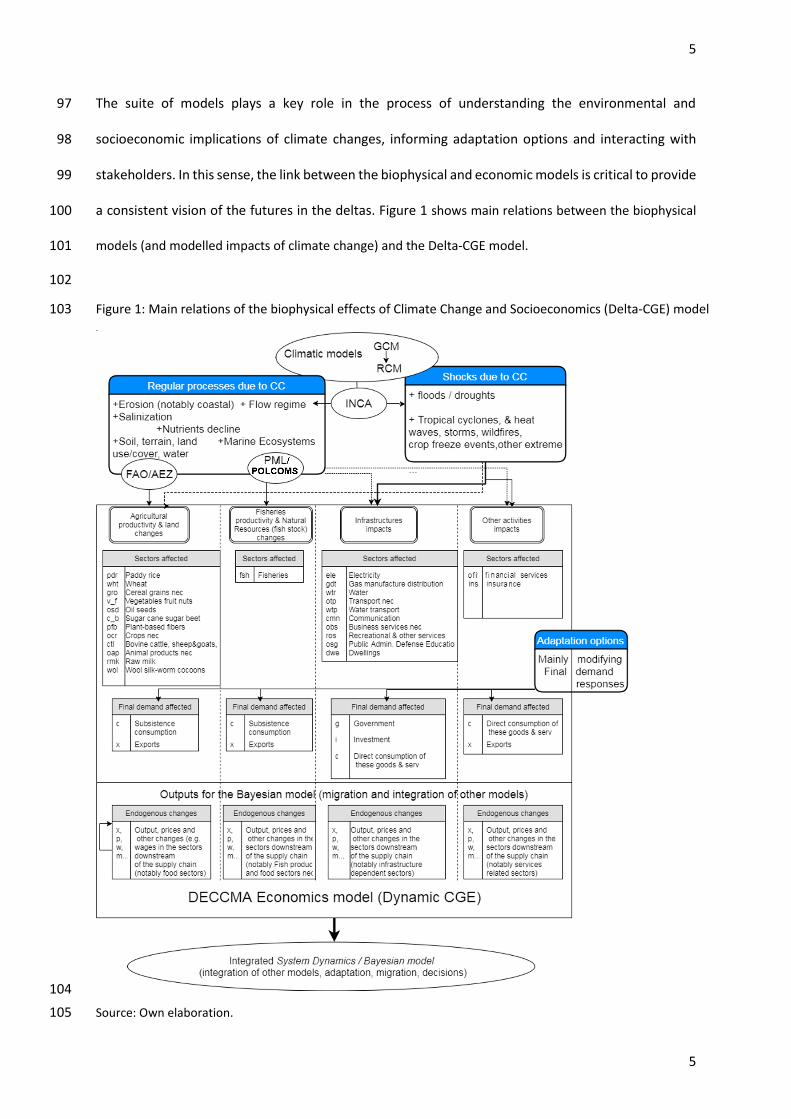
The suite of models plays a key role in the process of understanding the environmental and 97

socioeconomic implications of climate changes, informing adaptation options and interacting with 98

stakeholders. In this sense, the link between the biophysical and economic models is critical to provide 99

a consistent vision of the futures in the deltas. Figure 1 shows main relations between the biophysical 100

models (and modelled impacts of climate change) and the Delta-CGE model. 101

102

Figure 1: Main relations of the biophysical effects of Climate Change and Socioeconomics (Delta-CGE) model 103

104

Source: Own elaboration. 105

6

6

Starting from the top in Figure 1, we see the large-scale general circulation models (GCMs) which have 106

been used to simulate climate across the region and to assess the impacts of increasing greenhouse gas 107

concentrations on the global climate system4. These provide a starting point for the regional climate 108

models (RCMs), which dynamically downscale the results of the simulations with the GCMs5. CORDEX and 109

PRECISE have been used by the UK Met Office to downscale the results for Africa and South Asia 110

respectively (see Macadam et al, 2017 in this Special issue). 111

The set biophysical models take as inputs different outputs from the climate models provide. The INCA 112

hydrological model serves to generate information on biophysical processes and ecosystems taking 113

information form the climatic models. The model also makes use of some hypothesis on future evolution 114

of human-driven drivers with influence in hydrological processes such as population, public water use, 115

effluent discharge, water demand for irrigation and public supply, land use change, atmospheric deposition 116

or water transfer (Whitehead et al., 2017)). The results of the INCA model are further used by the crop and 117

fisheries models described below. 118

The FAO/AEZ (Agro-Ecological Zoning) modelling (Fischer et al., 2012; IIASA, 2018) is a comprehensive 119

framework accounting for climate, soil, terrain and management conditions matched with specific crop 120

requirements under different input levels and water supply. It provides a georeferenced database at 1 km 121

resolution of crop suitability and potential productivity for current (baseline conditions averaged over 30 122

years of observations) and future scenarios for major crops. From the economic perspective, the key output 123

from the model is the evaluation of current and future land suitability and the estimation of crop yields, 124

potential production and ecosystem services. 125

The POLCOMS-ERSEM biogeochemical model is used to drive a dynamic marine ecosystem model that 126

explicitly accounts for food web interactions by linking primary production to fish production through 127

predation. The model estimates potential for fish production by size class, taking into account temperature 128

effects on the feeding and intrinsic mortality rates of organisms (Blanchard et al. 2012). Hence it can make 129

4GCMs typically have coarse spatial resolutions with horizontal grid boxes of a few hundred kilometres, and cannot provide the high-resolution climate information that is required for climate impact and adaptation studies. 5Using boundary conditions from GCMs, and providing resolution grids of around 50km or smaller, typically representing

better features such as local topography and coast lines and their effects on the regional climate, such as rainfall.

7

7

climate-driven projections of changes in potential fish production. Size-based methods like this capture the 130

properties of food webs that describe energy flux and production at a particular size, independent of 131

species’ ecology (Barange et al., 2014). It also incorporates species interactions based on size-spectrum 132

theory and habitat suitability (Barange et al., 2013; Fernandes et al., 2017, 2016). Productivity changes then 133

are also derived for three GCMs in each delta. 134

As it can be seen in Figure 1, biophysical models produce information on the effects of changes in the 135

environmental conditions on some parameters such as crop yield, land availability or fisheries productivity 136

that affect the economic system. In this regard, the biophysical models serve as the between climatic 137

models and the economic model. 138

Data from the biophysical models, together with information on climate-related shocks directly affecting 139

the economic systems (e.g. damages in infrastructures due to floods) and adaption options are used by the 140

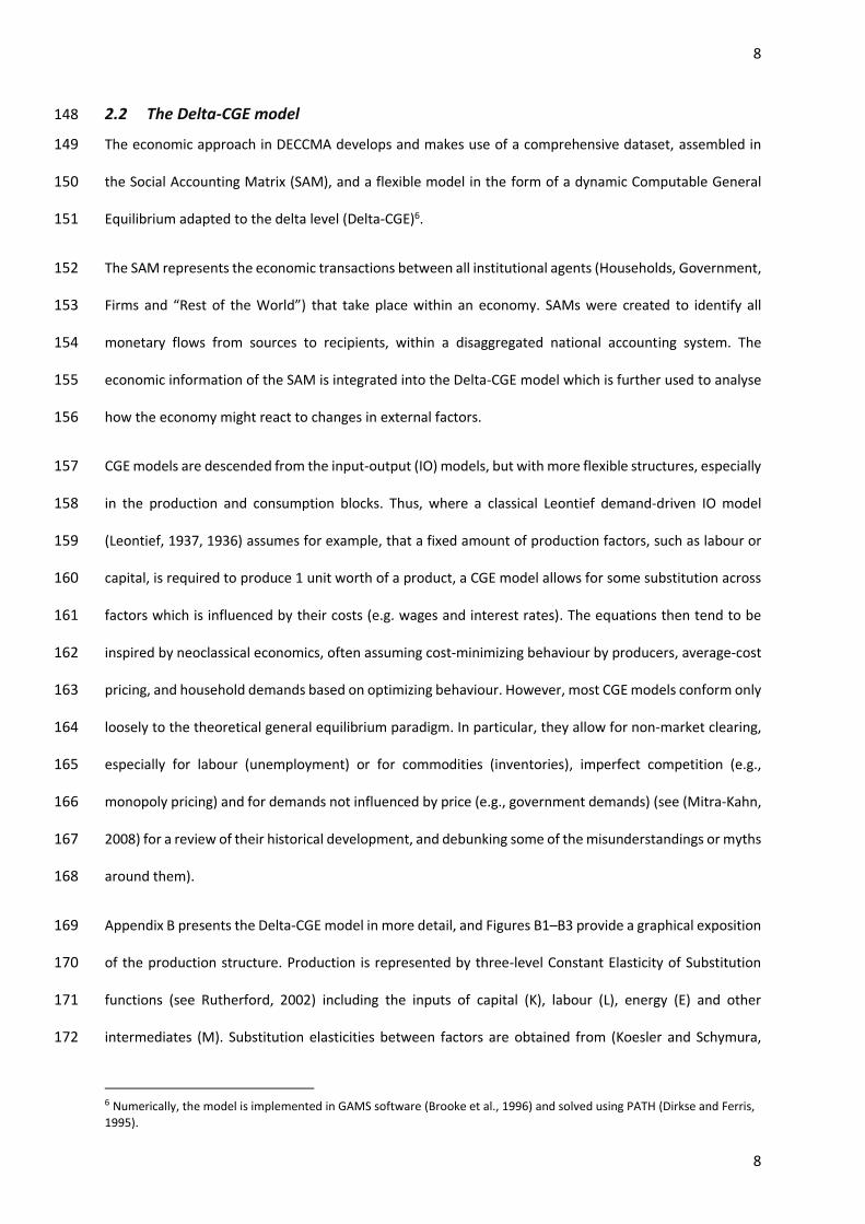
Delta-CGE model to analyse the economic implications of climate change in the deltas. Specifically, Table 141

1 shows the links between the variables of the biophysical models and the Delta-CGE model. Next, we 142

describe in detail the Delta-CGE model. 143

Table 1: Variables from other model components mapped to the variables of the CGE model 144

Model Variable in Model Variable in CGE

POLCOMS-ERSEM (PML)

Fisheries catch and output (physical, i.e. tons, and monetary, $, for the baseline) and endowment (physical units)

Fisheries output (monetary terms) and natural resources (fisheries cell) endowment (natural resources availability, in physical units)

Productivity change of fisheries (%, yearly up to 2050) Fisheries output change of (yearly up to 2050)

FAO/AEZ Cropland used and available area (ha, Baseline data) Cropland coefficient (use) and land endowment (Baseline data)

Cropland area potentials (ha, yearly up to 2050) Cropland endowment change (yearly up to 2050)

Crop output potentials (tons, yearly up to 2050) Crop output change (yearly up to 2050)

Source: Own elaboration. 145

146

147

8

8

2.2 The Delta-CGE model 148

The economic approach in DECCMA develops and makes use of a comprehensive dataset, assembled in 149

the Social Accounting Matrix (SAM), and a flexible model in the form of a dynamic Computable General 150

Equilibrium adapted to the delta level (Delta-CGE)6. 151

The SAM represents the economic transactions between all institutional agents (Households, Government, 152

Firms and “Rest of the World”) that take place within an economy. SAMs were created to identify all 153

monetary flows from sources to recipients, within a disaggregated national accounting system. The 154

economic information of the SAM is integrated into the Delta-CGE model which is further used to analyse 155

how the economy might react to changes in external factors. 156

CGE models are descended from the input-output (IO) models, but with more flexible structures, especially 157

in the production and consumption blocks. Thus, where a classical Leontief demand-driven IO model 158

(Leontief, 1937, 1936) assumes for example, that a fixed amount of production factors, such as labour or 159

capital, is required to produce 1 unit worth of a product, a CGE model allows for some substitution across 160

factors which is influenced by their costs (e.g. wages and interest rates). The equations then tend to be 161

inspired by neoclassical economics, often assuming cost-minimizing behaviour by producers, average-cost 162

pricing, and household demands based on optimizing behaviour. However, most CGE models conform only 163

loosely to the theoretical general equilibrium paradigm. In particular, they allow for non-market clearing, 164

especially for labour (unemployment) or for commodities (inventories), imperfect competition (e.g., 165

monopoly pricing) and for demands not influenced by price (e.g., government demands) (see (Mitra-Kahn, 166

2008) for a review of their historical development, and debunking some of the misunderstandings or myths 167

around them). 168

Appendix B presents the Delta-CGE model in more detail, and Figures B1–B3 provide a graphical exposition 169

of the production structure. Production is represented by three-level Constant Elasticity of Substitution 170

functions (see Rutherford, 2002) including the inputs of capital (K), labour (L), energy (E) and other 171

intermediates (M). Substitution elasticities between factors are obtained from (Koesler and Schymura, 172

6 Numerically, the model is implemented in GAMS software (Brooke et al., 1996) and solved using PATH (Dirkse and Ferris,

1995).

9

9

2015). In Figure B “Scheme of the elasticities” in Appendix B the scheme is illustrated, and a more in depth 173

review, and discussion on the functional forms, elasticities and key parameters of CGEs for sensitivity 174

testing is provided in the Appendix C. 175

As suggested by many growth models (Domar, 1946; Harrod, 1939; Romer, 1986; Solow, 1956; Swan, 1956) 176

savings and, subsequently, investments are the major determinants of long-term economic growth. Our 177

dynamics of capital accumulation equation follows (Dellink et al., 2004). The rate of return on investments 178

is determined on the domestic market, the capital stock and investment levels are fully endogenised, and 179

households decide the share of their income that is saved. These savings in turn are used by the producers 180

for capital investments and the rate of return on investments equals the exogenous interest rate. The 181

forward-looking behaviour of the agents and the endogenous savings rate make this a model of the 182

(Ramsey, 1928)-(Cass, 1965)-(Koopmans, 1965)- type (see (Barro and Sala-i-Martin, 1995; Carroll, 2017; 183

Heijdra, 2016). Total factor productivity growth is introduced, and adjusted to differentiate among 184

agriculture, industry and services, to reflect structural changes, as projected from the expert information 185

obtained from the questionnaires (see more in Appendix B and Figure B1). 186

Within the dynamic Delta-CGE model, the sets of labour types are divided as formal (related to the urban 187

employed) and informal (more related to the pool of labour from rural areas that does not have a “regular” 188

job, either temporally or permanently). The model assumes different wages for the different types of 189

labour and two additional constraints are added to the Delta-CGE model. The first is the “unemployment” 190

constraint determining the relative price of the formal labour. The second is the “mobility rate” constraint, 191

which also determines the relative wage of the informal labour to the formal labour, and which hence 192

establishes to what extent people will move due to an expected higher wage in the urban area (i.e. the 193

non-delta area). Finally, migration equations also take into account that, due to several costs, migration 194

does not occur when the difference between the “expected wages” are not large enough, and that mobility 195

does not occur if the initial wealth is not enough to cover migration costs (Lazar and Al., 2017; Safra de 196

Campos and Al., 2017a, 2017b))7. 197

7 The main reason for migration claimed (by the majority of respondents) is “search for employment”. In the Mahanadi also

the reason of join spouse/marriage is very important (around 20% of respondents), slightly above the reason of education.

10

10

Apart from the search of data for all these components, and especially for the calibration of the model, 198

within the economic modelling literature, and in particular in that of CGEs, sensitivity analyses tests are 199

partially conducted. Very rarely though are these done in a comprehensive way (typically rather in a 200

discrete way with a few variations) through Monte-Carlo simulations, with multiple combinations of values 201

of parameters, as has been done here. In this study we have explored wide ranges of possible values for 202

the parameters according to recent literature. A more in-depth discussion on the functional forms, 203

elasticities and key parameters of CGEs for sensitivity testing is provided in the Appendix C. 204

The database for the Delta-CGE model has been compiled from many sources and combines official 205

statistics with own estimations. As mentioned before, the IO tables of the deltas and associated SAM 206

constitute the core data of a Delta-CGE model (see (Arto and Cazcarro, 2017) and (Arto et al., 2018). 207

Appendix E (“IO and SAM elaboration”) describes the process of obtaining the SAM tables in DECCMA. The 208

main sources of information were different Regional/District datasets and analytical reports, such as the 209

census, specific information from industrial, agriculture and fisheries statistics in terms of production, value 210

added, employment, factor uses, intermediate consumption and final demand. In the case of MD, these 211

sources were the Primary Census and the Odisha Economic Surveys and agricultural statistics (GoO, 212

2016, 2015; PCA, 2011). Employment by district and gender (male/female) for the main 12 213

activities/sectors8 were compiled and further split into 57 sectors. At the national level, some small 214

corrections were applied to the employment data in order to obtain consistent wages. Other key data for 215

the construction of the database, in particular for the agricultural sector, are the agricultural land use, crop 216

and animal production, prices, data of livestock and fisheries stock and catches. 217

218

219

There is also a positively correlation in the migrant sending households with high in vulnerability (35%), being female headed household (13% of all), who furthermore takes further responsibility with the typical male migration. 8 Cultivators; Agricultural labourers; Plantation, Livestock, Forestry, Fishing, Hunting & allied activities; Mining & Quarrying;

Manufacturing; Electricity, Gas & Water Supply; Construction; Wholesale & Retail Trade; Hotels & Restaurants; Transport, Storage & Communications; Financial Intermediation, Real Estate, Renting & Business; Public Administration, Other Community, Social & Personal Services, Private Households Employing Persons.

11

11

3. Scenario framework 220

3.1 General overview 221

(Kebede et al., 2017), in this Special Issue, describe in detail the scenarios framework of DECCMA, which is 222

based on the new global scenario framework developed for the Fifth Assessment Report (AR5) of the IPCC. 223

The framework provides a foundation for an improved integrated assessment of climate change impacts 224

and adaptation and mitigation needs under a range of climate pathways, socioeconomic scenarios, and 225

adaptation and mitigation policy assumptions. For each of these three spheres the scientific community 226

has developed a set of quantitative and qualitative narratives, namely Representative Concentrations 227

Pathways, RCP (van Vuuren et al., 2011), Shared Socioeconomic Pathways, SSP (O’Neill et al., 2014)) and 228

Shared Policy Assumptions, SPA (Kriegler et al., 2014). 229

From the climatic perspective, DECCMA focuses on the RCP8.5 scenario in order to consider the strongest 230

climate (a ‘high-end’) signal, which shows the highest concentration of greenhouse gas concentrations in 231

the late 21st century. RCP 8.5 simulations (with three GCMs for each delta9) represent a worst-case end of 232

the 21st century projected temperature increases and atmospheric CO2 concentrations. In the case of the 233

FAO/AEZ the outputs are provided under climate scenario ensembles (ENS, that is to say, synthesized 234

results from combinations or averaging results from the different GCMs considered for each delta). 235

Up to 2050 the RCP8.5 was judged to be capable of being combined with practically any SSP (see (Riahi et 236

al., 2017), as high divergence of forcings from the different RCPs occur mainly beyond 2050s. However, 237

after 2050 only SSP3 and SSP5 can produce the required emissions, although SSP2 is close. Figure 5 in 238

(Kebede et al., 2017) presents a summary of the selected RCP and SSP scenario combinations and 239

associated time horizons considered for assessing different socioeconomic and biophysical components of 240

the delta systems investigated within DECCMA. 241

SSP3 presents a world of Fragmentation/Regional Rivalry (High mitigation and adaptation challenges), SSP5 242

presents a Conventional/Fossil-fuelled Development (High mitigation and low adaptation challenges), and 243

9 Using the French GCM, CNRM-CM5, and the UK GCM, HadGEM2-ES, both for Africa and South Asia. Then for South Asia

(see (IIASA, 2018) it is also used the German GCM, GFDL-CM3, and for Africa the CanESM2.

12

12

SSP2 is known as the Middle of the Road (Intermediate mitigation and adaptation challenges). Based on 244

this three SSP, in DECCMA three SSP-based scenario narratives have been identified up to 2050: Business 245

as Usual or Medium (SSP2), Medium– (SSP3) and Medium+ (SSP5). These narratives are then used to 246

downscale the global projections to regional and national levels, and to inform the development of the 247

participatory-based delta-scale scenarios and adaptation policy trajectories up to 2050. 248

It is important to highlight, that in the simulations, all these scenarios are considered as “baseline” 249

scenarios, in the sense that they assume that there is no climate change. In other words, climate change 250

shocks are simulated “on-top” of these three scenarios and the resulting economic effects are analysed in 251

terms of differences with respect the baseline scenario. 252

At the national scale, the socioeconomic scenarios for the three countries (Ghana, India, and Bangladesh) 253

are based on the SSP Public Database Version 1.110. This database provides historic trends and future 254

projections of the changes in population, share of population in urban areas, and GDP in power purchasing 255

parities (PPP) through the 21st century for each country under the five SSP scenarios (Figure 7 in (Kebede 256

et al., 2017). Together, these data are used as one of the boundary conditions to inform the development 257

of the delta-scale scenarios, that were developed with the support of experts through questionnaires. 258

GDP is one of the few economic measures which are numerically estimated and projected for the different 259

SSPs different futures. 260

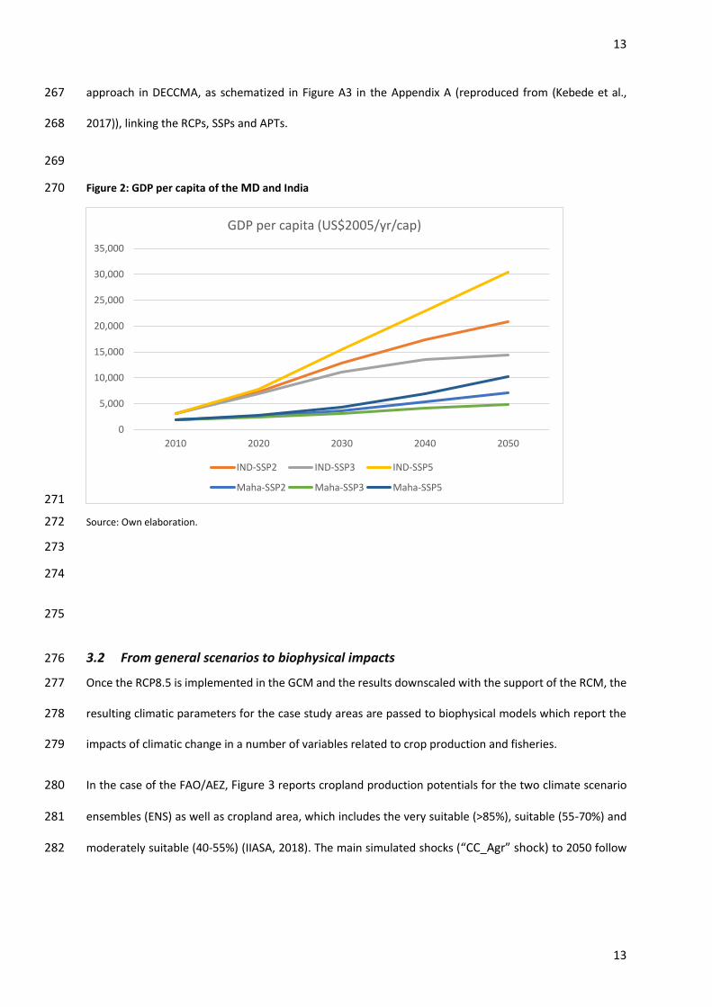
Figure 2 shows the ranges of paths of growth of the GDP per capita for the India and the MD for the 261

different SSPs. We may observe how the gap between the regions increases over time, something which 262

contributes to increase out migration from the delta. 263

Apart from the RCPs and SSPs, a number of adaptation policy trajectories (ATPs), inspired in the SPA, are 264

also taken into account in order to provide a complete view of the possible futures in the deltas. Indeed, 265

these futures may be radically different depending on the adaption pathways selected. This leads us to an 266

10See: https://secure.iiasa.ac.at/web-apps/ene/SspDb

13

13

approach in DECCMA, as schematized in Figure A3 in the Appendix A (reproduced from (Kebede et al., 267

2017)), linking the RCPs, SSPs and APTs. 268

269

Figure 2: GDP per capita of the MD and India 270

271

Source: Own elaboration. 272

273

274

275

3.2 From general scenarios to biophysical impacts 276

Once the RCP8.5 is implemented in the GCM and the results downscaled with the support of the RCM, the 277

resulting climatic parameters for the case study areas are passed to biophysical models which report the 278

impacts of climatic change in a number of variables related to crop production and fisheries. 279

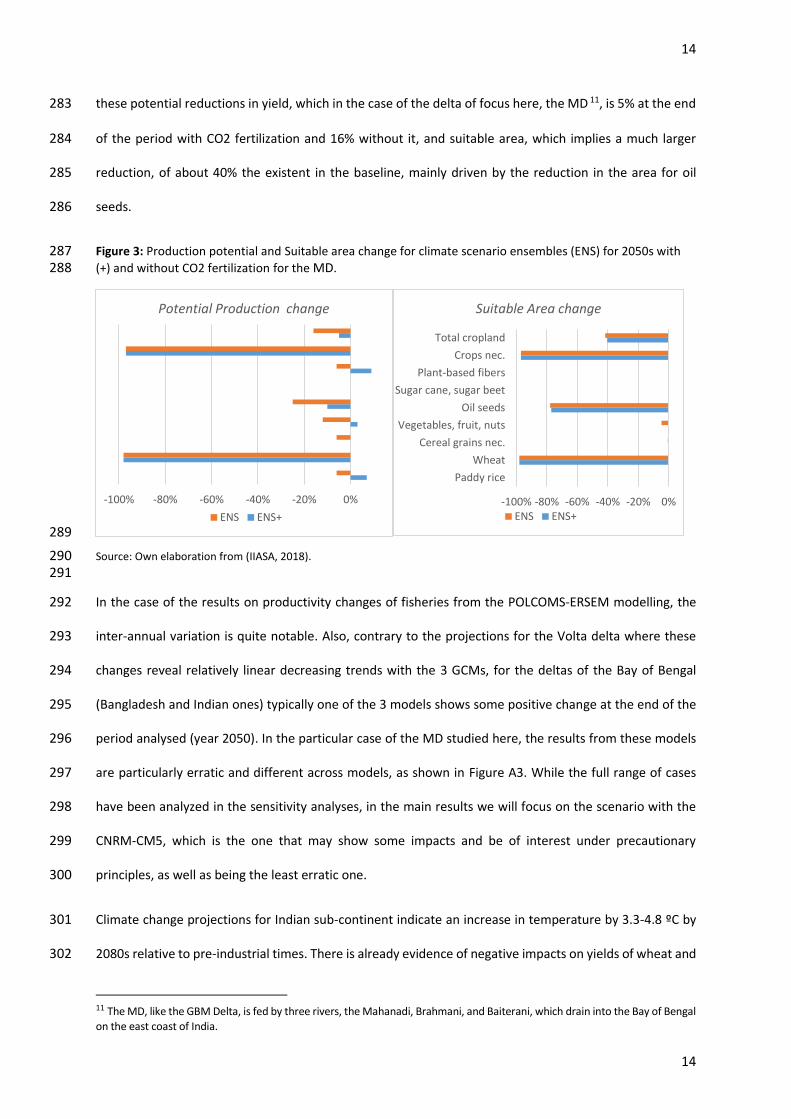
In the case of the FAO/AEZ, Figure 3 reports cropland production potentials for the two climate scenario 280

ensembles (ENS) as well as cropland area, which includes the very suitable (>85%), suitable (55-70%) and 281

moderately suitable (40-55%) (IIASA, 2018). The main simulated shocks (“CC_Agr” shock) to 2050 follow 282

0

5,000

10,000

15,000

20,000

25,000

30,000

35,000

2010 2020 2030 2040 2050

GDP per capita (US$2005/yr/cap)

IND-SSP2 IND-SSP3 IND-SSP5

Maha-SSP2 Maha-SSP3 Maha-SSP5

14

14

these potential reductions in yield, which in the case of the delta of focus here, the MD 11, is 5% at the end 283

of the period with CO2 fertilization and 16% without it, and suitable area, which implies a much larger 284

reduction, of about 40% the existent in the baseline, mainly driven by the reduction in the area for oil 285

seeds. 286

Figure 3: Production potential and Suitable area change for climate scenario ensembles (ENS) for 2050s with 287 (+) and without CO2 fertilization for the MD. 288

289

Source: Own elaboration from (IIASA, 2018). 290 291

In the case of the results on productivity changes of fisheries from the POLCOMS-ERSEM modelling, the 292

inter-annual variation is quite notable. Also, contrary to the projections for the Volta delta where these 293

changes reveal relatively linear decreasing trends with the 3 GCMs, for the deltas of the Bay of Bengal 294

(Bangladesh and Indian ones) typically one of the 3 models shows some positive change at the end of the 295

period analysed (year 2050). In the particular case of the MD studied here, the results from these models 296

are particularly erratic and different across models, as shown in Figure A3. While the full range of cases 297

have been analyzed in the sensitivity analyses, in the main results we will focus on the scenario with the 298

CNRM-CM5, which is the one that may show some impacts and be of interest under precautionary 299

principles, as well as being the least erratic one. 300

Climate change projections for Indian sub-continent indicate an increase in temperature by 3.3-4.8 ºC by 301

2080s relative to pre-industrial times. There is already evidence of negative impacts on yields of wheat and 302

11 The MD, like the GBM Delta, is fed by three rivers, the Mahanadi, Brahmani, and Baiterani, which drain into the Bay of Bengal

on the east coast of India.

-100% -80% -60% -40% -20% 0%

Potential Production change

ENS ENS+

-100% -80% -60% -40% -20% 0%

Paddy rice

Wheat

Cereal grains nec.

Vegetables, fruit, nuts

Oil seeds

Sugar cane, sugar beet

Plant-based fibers

Crops nec.

Total cropland

Suitable Area change

ENS ENS+

15

15

paddy in some parts of India due to increased temperature, water stress and reduction in number of rainy 303

days. In the medium-term (2020–2039), crop yield is projected to reduce by 4.5 to 9%, depending on the 304

magnitude and distribution of warming (NICRA, 2013). More general projections from combinations of data 305

points from crop model projections indicate decreases of between 10-25% in yield by 2050 in a RCP8.5 306

scenario (see Figure 2.7 of the IPCC AR5, (IPCC, 2014)). This implies up to around 0.5% loss per year, and so 307

we will also examine such paths in the Sensitivity analysis section. 308

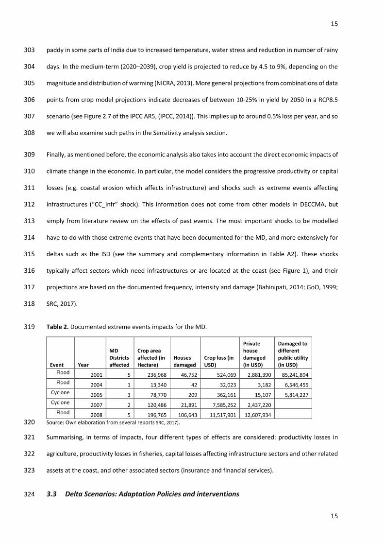
Finally, as mentioned before, the economic analysis also takes into account the direct economic impacts of 309

climate change in the economic. In particular, the model considers the progressive productivity or capital 310

losses (e.g. coastal erosion which affects infrastructure) and shocks such as extreme events affecting 311

infrastructures (“CC_Infr” shock). This information does not come from other models in DECCMA, but 312

simply from literature review on the effects of past events. The most important shocks to be modelled 313

have to do with those extreme events that have been documented for the MD, and more extensively for 314

deltas such as the ISD (see the summary and complementary information in Table A2). These shocks 315

typically affect sectors which need infrastructures or are located at the coast (see Figure 1), and their 316

projections are based on the documented frequency, intensity and damage (Bahinipati, 2014; GoO, 1999; 317

SRC, 2017). 318

Table 2. Documented extreme events impacts for the MD. 319

Event Year

MD Districts affected

Crop area affected (in Hectare)

Houses damaged

Crop loss (in USD)

Private house damaged (in USD)

Damaged to different public utility (in USD)

Flood 2001 5 236,968 46,752 524,069 2,881,390 85,241,894

Flood 2004 1 13,340 42 32,023 3,182 6,546,455

Cyclone 2005 3 78,770 209 362,161 15,107 5,814,227

Cyclone 2007 2 120,486 21,891 7,585,252 2,437,220

Flood 2008 5 196,765 106,643 11,517,901 12,607,934

Source: Own elaboration from several reports SRC, 2017). 320

Summarising, in terms of impacts, four different types of effects are considered: productivity losses in 321

agriculture, productivity losses in fisheries, capital losses affecting infrastructure sectors and other related 322

assets at the coast, and other associated sectors (insurance and financial services). 323

3.3 Delta Scenarios: Adaptation Policies and interventions 324

16

16

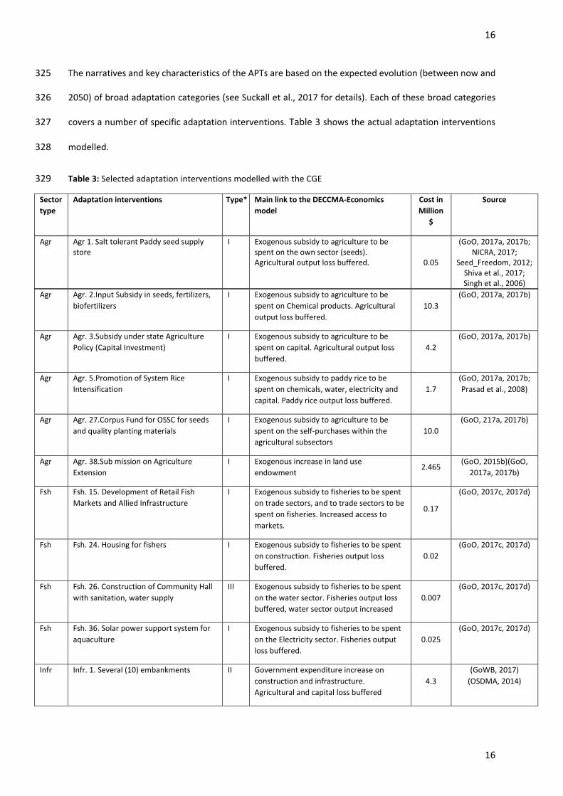
The narratives and key characteristics of the APTs are based on the expected evolution (between now and 325

2050) of broad adaptation categories (see Suckall et al., 2017 for details). Each of these broad categories 326

covers a number of specific adaptation interventions. Table 3 shows the actual adaptation interventions 327

modelled. 328

Table 3: Selected adaptation interventions modelled with the CGE 329

Sector

type

Adaptation interventions Type* Main link to the DECCMA-Economics

model Cost in

Million

$

Source

Agr Agr 1. Salt tolerant Paddy seed supply store

I Exogenous subsidy to agriculture to be spent on the own sector (seeds). Agricultural output loss buffered. 0.05

(GoO, 2017a, 2017b; NICRA, 2017;

Seed_Freedom, 2012; Shiva et al., 2017; Singh et al., 2006)

Agr Agr. 2.Input Subsidy in seeds, fertilizers,

biofertilizers I Exogenous subsidy to agriculture to be

spent on Chemical products. Agricultural

output loss buffered. 10.3

(GoO, 2017a, 2017b)

Agr Agr. 3.Subsidy under state Agriculture

Policy (Capital Investment) I Exogenous subsidy to agriculture to be

spent on capital. Agricultural output loss

buffered. 4.2

(GoO, 2017a, 2017b)

Agr Agr. 5.Promotion of System Rice

Intensification I Exogenous subsidy to paddy rice to be

spent on chemicals, water, electricity and

capital. Paddy rice output loss buffered. 1.7

(GoO, 2017a, 2017b;

Prasad et al., 2008)

Agr Agr. 27.Corpus Fund for OSSC for seeds

and quality planting materials I Exogenous subsidy to agriculture to be

spent on the self-purchases within the

agricultural subsectors 10.0

(GoO, 217a, 2017b)

Agr Agr. 38.Sub mission on Agriculture

Extension I Exogenous increase in land use

endowment 2.465

(GoO, 2015b)(GoO,

2017a, 2017b)

Fsh Fsh. 15. Development of Retail Fish

Markets and Allied Infrastructure I Exogenous subsidy to fisheries to be spent

on trade sectors, and to trade sectors to be

spent on fisheries. Increased access to

markets.

0.17

(GoO, 2017c, 2017d)

Fsh Fsh. 24. Housing for fishers I Exogenous subsidy to fisheries to be spent

on construction. Fisheries output loss

buffered.

0.02

(GoO, 2017c, 2017d)

Fsh Fsh. 26. Construction of Community Hall

with sanitation, water supply

III Exogenous subsidy to fisheries to be spent

on the water sector. Fisheries output loss

buffered, water sector output increased

0.007

(GoO, 2017c, 2017d)

Fsh Fsh. 36. Solar power support system for

aquaculture

I Exogenous subsidy to fisheries to be spent

on the Electricity sector. Fisheries output

loss buffered.

0.025

(GoO, 2017c, 2017d)

Infr Infr. 1. Several (10) embankments II Government expenditure increase on

construction and infrastructure.

Agricultural and capital loss buffered

4.3

(GoWB, 2017)

(OSDMA, 2014)

17

17

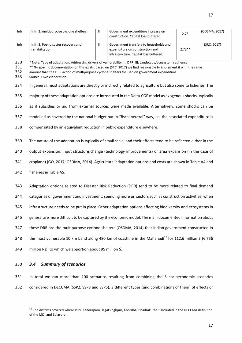
Infr Infr. 2. multipurpose cyclone shelters II Government expenditure increase on

construction. Capital loss buffered. 2.73

(ODSMA, 2017)

Infr Infr. 3. Post-disaster recovery and

rehabilitation

II Government transfers to households and

expenditure on construction and

infrastructure. Capital loss buffered.

2.73**

(SRC, 2017)

* Note: Type of adaptation. Addressing drivers of vulnerability; II. DRR, III. Landscape/ecosystem resilience. 330 ** No specific documentation on this exists, based on (SRC, 2017) we find reasonable to implement it with the same 331 amount than the DRR action of multipurpose cyclone shelters focused on government expenditure. 332 Source: Own elaboration. 333

In general, most adaptations are directly or indirectly related to agriculture but also some to fisheries. The 334

majority of these adaptation options are introduced in the Delta-CGE model as exogenous shocks, typically 335

as if subsidies or aid from external sources were made available. Alternatively, some shocks can be 336

modelled as covered by the national budget but in “fiscal neutral” way, i.e. the associated expenditure is 337

compensated by an equivalent reduction in public expenditure elsewhere. 338

The nature of the adaptation is typically of small scale, and their effects tend to be reflected either in the 339

output expansion, input structure change (technology improvements) or area expansion (in the case of 340

cropland) (GO, 2017; OSDMA, 2014). Agricultural adaptation options and costs are shown in Table A4 and 341

fisheries in Table A5. 342

Adaptation options related to Disaster Risk Reduction (DRR) tend to be more related to final demand 343

categories of government and investment, spending more on sectors such as construction activities, when 344

infrastructure needs to be put in place. Other adaptation options affecting biodiversity and ecosystems in 345

general are more difficult to be captured by the economic model. The main documented information about 346

these DRR are the multipurpose cyclone shelters (OSDMA, 2014) that Indian government constructed in 347

the most vulnerable 10 km band along 480 km of coastline in the Mahanadi12 for 112.6 million $ (6,756 348

million Rs), to which we apportion about 95 million $. 349

3.4 Summary of scenarios 350

In total we ran more than 100 scenarios resulting from combining the 3 socioeconomic scenarios 351

considered in DECCMA (SSP2, SSP3 and SSP5), 3 different types (and combinations of them) of effects or 352

12 The districts covered where Puri, Kendrapara, Jagatsinghpur, Khordha, Bhadrak (the 5 included in the DECCMA definition

of the MD) and Balasore.

18

18

shocks induced by climate change, and 12 specific adaption interventions. Furthermore, CGE model 353

simulations are usually accompanied by sensitivity analyses in terms of specific model parameters which 354

are considered difficult to measure (such as elasticities) and, therefore, it is highly convenient to evaluate 355

their role in varying the results. For all these, we implemented a Monte Carlo analysis in order to run all 356

these possible combinations of variables and parameters. Apart from testing the uncertainty on some key 357

parameters of the economic model, we also requested the biophysical modellers to provide us with ranges 358

(if possible distributions) for the main climatic impacts from the biophysical models, that were included in 359

the Monte Carlo analysis. The parameters for which we perform the Monte Carlo analysis are shown in 360

Table A6 in the SM. 361

4. Results and sensitivity 362

4.1 Future economic impacts of climate change in the MD 363

364

The following results illustrate the economic implications of a combination of climatic, socioeconomic and 365

adaptation scenarios for the MD and for the whole India. We use as headline indicator the change in the 366

GDP per capita due to climate change with respect the scenario without climatic impacts. For the sake of 367

simplicity, in terms of socioeconomic scenarios, we just present the results of the SSP2 scenario, which is 368

referred as Business As Usual (BAU). On top of this BAU, the different shocks described in the previous 369

section are implemented and analysed. Finally, we provide a sensitivity analysis of simulated shocks. 370

In the following we examine the Cumulative Changes in macroeconomic variables from Climate Change 371

shocks for the Mahanadi Delta with respect to BAU (up to 2050). 372

373

Climate Change (CC) shocks with respect to BAU scenario for the Mahanadi delta 374

375

Based on the SSP2 scenario for the Mahanadi delta and India (grey line in Figure 2 above) and also for 376

the Mahanadi delta, which we call BAU, we examine the projected shocks described in previous 377

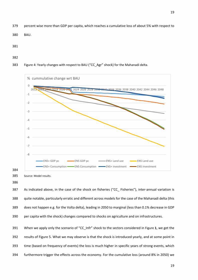
section. We may see in Figure 4 the “CC_Agr” shock, in which both consumption and investment fall 378

19

19

percent wise more than GDP per capita, which reaches a cumulative loss of about 5% with respect to 379

BAU. 380

381

382

Figure 4: Yearly changes with respect to BAU (“CC_Agr” shock) for the Mahanadi delta. 383

384

Source: Model results. 385

386

As indicated above, in the case of the shock on fisheries (“CC_ Fisheries”), inter-annual variation is 387

quite notable, particularly erratic and different across models for the case of the Mahanadi delta (this 388

does not happen e.g. for the Volta delta), leading in 2050 to marginal (less than 0.1% decrease in GDP 389

per capita with the shock) changes compared to shocks on agriculture and on infrastructures. 390

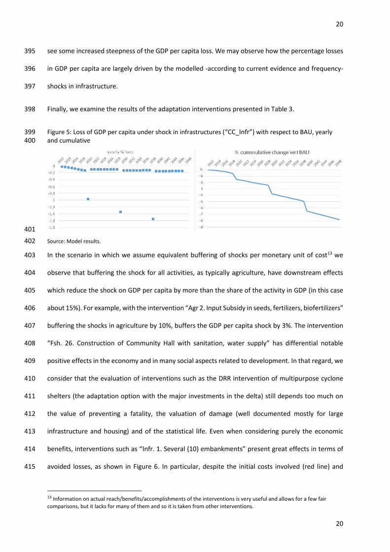
When we apply only the scenario of “CC_Infr” shock to the sectors considered in Figure 1, we get the 391

results of Figure 5. What we may observe is that the shock is introduced yearly, and at some point in 392

time (based on frequency of events) the loss is much higher in specific years of strong events, which 393

furthermore trigger the effects across the economy. For the cumulative loss (around 8% in 2050) we 394

-8

-7

-6

-5

-4

-3

-2

-1

0

2012 2014 2016 2018 2020 2022 2024 2026 2028 2030 2032 2034 2036 2038 2040 2042 2044 2046 2048

% cummulative change wrt BAU

ENS+ GDP pc ENS GDP pc ENS+ Land use ENS Land use

ENS+ Consumption ENS Consumption ENS+ investment ENS investment

20

20

see some increased steepness of the GDP per capita loss. We may observe how the percentage losses 395

in GDP per capita are largely driven by the modelled -according to current evidence and frequency- 396

shocks in infrastructure. 397

Finally, we examine the results of the adaptation interventions presented in Table 3. 398

Figure 5: Loss of GDP per capita under shock in infrastructures (“CC_Infr”) with respect to BAU, yearly 399 and cumulative 400

401

Source: Model results. 402

In the scenario in which we assume equivalent buffering of shocks per monetary unit of cost13 we 403

observe that buffering the shock for all activities, as typically agriculture, have downstream effects 404

which reduce the shock on GDP per capita by more than the share of the activity in GDP (in this case 405

about 15%). For example, with the intervention “Agr 2. Input Subsidy in seeds, fertilizers, biofertilizers” 406

buffering the shocks in agriculture by 10%, buffers the GDP per capita shock by 3%. The intervention 407

“Fsh. 26. Construction of Community Hall with sanitation, water supply” has differential notable 408

positive effects in the economy and in many social aspects related to development. In that regard, we 409

consider that the evaluation of interventions such as the DRR intervention of multipurpose cyclone 410

shelters (the adaptation option with the major investments in the delta) still depends too much on 411

the value of preventing a fatality, the valuation of damage (well documented mostly for large 412

infrastructure and housing) and of the statistical life. Even when considering purely the economic 413

benefits, interventions such as “Infr. 1. Several (10) embankments” present great effects in terms of 414

avoided losses, as shown in Figure 6. In particular, despite the initial costs involved (red line) and 415

13 Information on actual reach/benefits/accomplishments of the interventions is very useful and allows for a few fair

comparisons, but it lacks for many of them and so it is taken from other interventions.

21

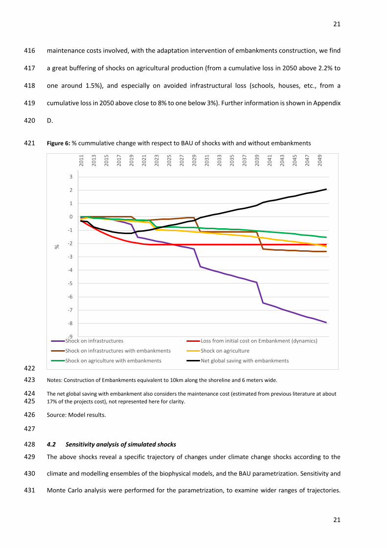
21

maintenance costs involved, with the adaptation intervention of embankments construction, we find 416

a great buffering of shocks on agricultural production (from a cumulative loss in 2050 above 2.2% to 417

one around 1.5%), and especially on avoided infrastructural loss (schools, houses, etc., from a 418

cumulative loss in 2050 above close to 8% to one below 3%). Further information is shown in Appendix 419

D. 420

Figure 6: % cummulative change with respect to BAU of shocks with and without embankments 421

422

Notes: Construction of Embankments equivalent to 10km along the shoreline and 6 meters wide. 423

The net global saving with embankment also considers the maintenance cost (estimated from previous literature at about 424 17% of the projects cost), not represented here for clarity. 425

Source: Model results. 426

427

4.2 Sensitivity analysis of simulated shocks 428

The above shocks reveal a specific trajectory of changes under climate change shocks according to the 429

climate and modelling ensembles of the biophysical models, and the BAU parametrization. Sensitivity and 430

Monte Carlo analysis were performed for the parametrization, to examine wider ranges of trajectories. 431

-9

-8

-7

-6

-5

-4

-3

-2

-1

0

1

2

3

20

11

20

13

20

15

20

17

20

19

20

21

20

23

20

25

20

27

20

29

20

31

20

33

20

35

20

37

20

39

20

41

20

43

20

45

20

47

20

49

%

Shock on infrastructures Loss from initial cost on Embankment (dynamics)

Shock on infrastructures with embankments Shock on agriculture

Shock on agriculture with embankments Net global saving with embankments

22

22

“Appendix D. Complementary results” of the SM summarizes these analyses. We found that in order to 432

understand the growth of GDP (PPP) and GDP per capita, the most sensitive parameters were total factor 433

productivity and population pathways, followed by the interest rates and the assumptions on the 434

production functions and trade. The changes in interest and depreciation rates were also highly influential 435

in the evolution of capital, investments, and in general in the performance of adaptation options focused 436

on Disaster Risk Reduction. 437

For the sake of comparison of the size of the resulting changes, we also ran ranges of shocks from climate 438

change for those same biophysical models. For example, the analogous figure to Figure 4 of a yearly 0.5% 439

shock with respect to BAU in agricultural land cover is shown in Figure D1. 440

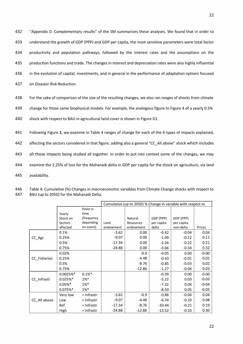
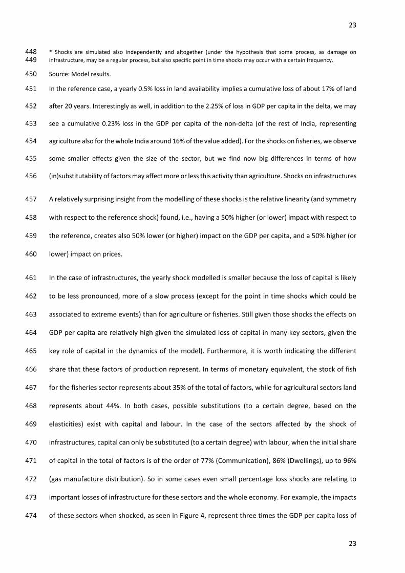
Following Figure 1, we examine in Table 4 ranges of change for each of the 4 types of impacts explained, 441

affecting the sectors considered in that figure, adding also a general “CC_All above” shock which includes 442

all those impacts being studied all together. In order to put into context some of the changes, we may 443

examine the 2.25% of loss for the Mahanadi delta in GDP per capita for the shock on agriculture, via land 444

availability. 445

Table 4: Cumulative (%) Changes in macroeconomic variables from Climate Change shocks with respect to 446 BAU (up to 2050) for the Mahanadi Delta. 447

Cumulative (up to 2050) % Change in variable with respect to BAU (reference path without shocks)

Yearly Shock on Sectors affected

Point in time (frequency depending on event) Shock

Land endowment

Natural Resources endowment

GDP (PPP) per capita delta

GDP (PPP) per capita non-delta Prices

CC_Agr

0.1% -3.62 0.00 -0.42 -0.04 0.04 0.25% -9.07 0.00 -1.09 -0.12 0.11

0.5% -17.34 0.00 -2.26 -0.22 0.21

0.75% -24.88 0.00 -3.66 -0.34 0.32

CC_Fisheries 0.02% -0.9 -0.05 0.00 -0.00 0.25% -4.48 -0.43 -0.01 0.01

0.5% -8.76 -0.85 -0.03 0.02

0.75% -12.86 -1.27 -0.04 0.03

0.0025%* 0.1%* -0.39 0.00 -0.00 CC_Infrastr 0.025%* 1%* -5.22 0.03 -0.03

0.05%* 1%* -7.32 0.04 -0.04

0.075%* 1%* -8.50 0.05 -0.05

CC_All above

Very low = Infrastr -3.62 -0.9 -0.86 -0.04 0.04

Low = Infrastr -9.07 -4.48 -6.74 -0.10 0.08

Ref = Infrastr -17.34 -8.76 -10.44 -0.21 0.19

High = Infrastr -24.88 -12.86 -13.52 -0.33 0.30

23

23

* Shocks are simulated also independently and altogether (under the hypothesis that some process, as damage on 448 infrastructure, may be a regular process, but also specific point in time shocks may occur with a certain frequency. 449

Source: Model results. 450

In the reference case, a yearly 0.5% loss in land availability implies a cumulative loss of about 17% of land 451

after 20 years. Interestingly as well, in addition to the 2.25% of loss in GDP per capita in the delta, we may 452

see a cumulative 0.23% loss in the GDP per capita of the non-delta (of the rest of India, representing 453

agriculture also for the whole India around 16% of the value added). For the shocks on fisheries, we observe 454

some smaller effects given the size of the sector, but we find now big differences in terms of how 455

(in)substitutability of factors may affect more or less this activity than agriculture. Shocks on infrastructures 456

A relatively surprising insight from the modelling of these shocks is the relative linearity (and symmetry 457

with respect to the reference shock) found, i.e., having a 50% higher (or lower) impact with respect to 458

the reference, creates also 50% lower (or higher) impact on the GDP per capita, and a 50% higher (or 459

lower) impact on prices. 460

In the case of infrastructures, the yearly shock modelled is smaller because the loss of capital is likely 461

to be less pronounced, more of a slow process (except for the point in time shocks which could be 462

associated to extreme events) than for agriculture or fisheries. Still given those shocks the effects on 463

GDP per capita are relatively high given the simulated loss of capital in many key sectors, given the 464

key role of capital in the dynamics of the model). Furthermore, it is worth indicating the different 465

share that these factors of production represent. In terms of monetary equivalent, the stock of fish 466

for the fisheries sector represents about 35% of the total of factors, while for agricultural sectors land 467

represents about 44%. In both cases, possible substitutions (to a certain degree, based on the 468

elasticities) exist with capital and labour. In the case of the sectors affected by the shock of 469

infrastructures, capital can only be substituted (to a certain degree) with labour, when the initial share 470

of capital in the total of factors is of the order of 77% (Communication), 86% (Dwellings), up to 96% 471

(gas manufacture distribution). So in some cases even small percentage loss shocks are relating to 472

important losses of infrastructure for these sectors and the whole economy. For example, the impacts 473

of these sectors when shocked, as seen in Figure 4, represent three times the GDP per capita loss of 474

24

24

the agricultural sectors, and about 27 times more than the fisheries sectors, even though both of these 475

activities are greatly important in the delta and for the livelihoods of much of population. We also see 476

in Table 4 from the last 3 rows of shocks taken together that all the climate change related changes 477

considered, result (for the delta only) in cumulative (up to 2050) percentage losses in GDP per capita 478

with respect to BAU of about 11% for the delta, while barely of 0.25% nationally. 479

480

5. Conclusions 481

In this paper we have developed the conceptual and practical links between the climate, biophysical and 482

socioeconomics model in DECCMA. In particular, we have focused on the background and the 483

conceptualisation of the links between the global climate (RCPs) and socioeconomic (SSPs) scenario 484

narratives and policy assumptions (SPAs) for developing appropriate adaptation policy trajectories and 485

associated specific interventions in the deltas. The review of the literature shows how biophysical-486

economic models represent a diversity of approaches to describing human-nature interactions. Following 487

the line of dynamic CGE models which connect with other Partial Equilibrium, biophysical, crop/hydro/(…) 488

models in this framework we have translated the biophysical changes (coming from simulations with a 489

specific RCP 8.5) into changes in our dynamic economic model (Delta-CGE). Furthermore, we have 490

incorporated national and regional scenarios (3 SSPs) and adaptation policy alternatives which have 491

reasonable translations to our parameters or variables. 492

Our model is set up to incorporate the outputs from various biophysical models, harmonizing results into 493

common metrics to be used as inputs in the economic models. Similarly to the recognition explained in 494

(Wiebe et al., 2015), obtaining these variables under a high emissions pathway allows us to study and 495

highlight how production and food security may be affected by climate change from various perspectives. 496

Furthermore, it can examine the impacts of climate change on yields, production, area, prices, and trade 497

across multiple socioeconomic and policy pathways. For this reason, despite some possible feedbacks 498

among variables which ideally could be captured with the integrated framework of the project, the 499

25

25

DECCMA Economics model already represents the natural next step or way forward of analysing 500

biophysical impacts further in the supply chains. 501

Indeed, the main design of the model and scenarios analysis has been done so that the robust Monte-Carlo 502

type runs create an “emulator” which can be implemented in the integrated (Bayesian type) framework of 503

the project. In this regard, we have performed a wide sensitivity analysis on how the endogenous variables 504

in the model respond to the main parameters and exogenous information which enters it as inputs. In 505

particular, we found that in order to understand the growth of GDP, the most sensitive parameters were 506

total factor productivity and population pathways, followed by the interest rates and the assumptions on 507

the production functions and trade. The modelling of the climate change impacts via loss of land 508

dramatically affected more the agricultural outputs and GDP in general than the specification via 509

productivity losses. The changes in interest and depreciation rates were also highly influential in the 510

evolution of capital, investments, and in general in the performance of adaptation options focused on 511

Disaster Risk Reduction. As also found in (Eboli et al., 2010), one may also observe how second-order, 512

system-wide effects of climate change impacts typically have significant distributional effects at the 513

regional and industrial level. The interaction between endogenous and exogenous dynamics generates 514

non-linear deviations from the baseline, amplifying or counteracting exogenous shocks on the long run. 515

The main future steps with the DECCMA Economics modelling have to do with this further validation, and 516

with the implementation with much more data on scenarios, coming from all the different (notably the 517

biophysical, but also from the integrated Bayesian) models results, and implemented for all the deltas 518

under study in DECCMA. Inter-comparison of results should also serve us to further disentangle how the 519

choice of parameters affects the results, and in general the uncertainty of the modelling. Probably even 520

more importantly, we should then be able to fully address how the variables evolve, to be able to provide 521

comprehensive measures on output, prices, welfare, income or wages, for each of the scenarios and 522

adaptation options, hopefully provide guidance on the socioeconomic implications of the different choices, 523

and on specific policy implications, such as the positive effects found here of specific adaptation 524

interventions, namely the input subsidies in seeds and fertilizers, and the DRR interventions of building 525

multipurpose cyclone shelters and constructing embankments. Also possible future distinction of 526

26

26

socioeconomic groups (from the Social Accounting Matrices) may serve us to differentiate impacts on 527

vulnerable groups, based on their different patterns on migration and vulnerability to climate change, 528

leading to interesting results and discussion on distributional issues and policy measures. 529

530 531 532 533

Acknowledgements 534

This work was carried out under the DEltas, vulnerability and Climate Change: Migration and 535

Adaptation (DECCMA) project which is part of Collaborative Adaptation Research Initiative in Africa 536

and Asia (CARIAA), with financial support from the UK Government’s Department for International 537

Development (DfID) and the International Development Research Centre (IDRC), Canada. The views 538

expressed in this work are those of the creators and do not necessarily represent those of DfID and 539

IDRC or its Board of Governors. 540

541

References 542

Adams, H., Mortreux, C., Adger, N., Safra de Campos, R., Team, W., 2017. Successful migration across systems. 543

Arto, I., Cazcarro, I., 2017. Hybrid (survey and non-survey) methods for the construction of subnational/regional IO tables 544 with insights for their construction for Deltaic environments. 545

Arto, I., Cazcarro, I., Hazra, S., Bhattacharya, R.N., Adjei, Osei-Wusu, P., Ofori-Danson, P.K., Asenso, J.K., Amponsah, S.K., 546 Khondker, B., Raihan, S., Hossen, Z., 2018. Biophysical and socioeconomic state and links of deltaic areas vulnerable 547 to Climate Change from the perspectives of gender and spatial relations. 548

Bahinipati, C.S., 2014. Assessment of vulnerability to cyclones and floods in Odisha, India: A district-level analysis. Curr. Sci. 549 107, 1997–2007. 550

Barange, M., Fernandes, J., Kay, S., Parr, H., Ahmed, M., Hossain, M., 2013. Contribution and long-term future of marine 551 fisheries as providers of food and income in Bangladesh: a modelling study. 552

Barange, M., Merino, G., Blanchard, J.L., Scholtens, J., Harle, J., Allison, E.H., Allen, J.I., Holt, J., Jennings, S., 2014. Impacts 553 of climate change on marine ecosystem production in societies dependent on fisheries. Nat. Clim. Chang. 4, 211. 554

Barro, R.J., Sala-i-Martin, X., 1995. Economic Growth. McGraw-Hill, Inc, New York. 555

Blanchard, J.L., Jennings, S., Holmes, R., Harle, J., Merino, G., Allen, J.I., Holt, J., Dulvy, N.K., Barange, M., 2012. Potential 556 consequences of climate change for primary production and fish production in large marine ecosystems. Philos. 557 Trans. R. Soc. B Biol. Sci. 367, 2979 LP-2989. 558

Brooke, A., Kendrick, D., Meeraus., A., 1996. GAMS: A User’s Guide. Washington, DC, DC. 559

Burke, M., Hsiang, S.M., Miguel, E., 2015. Global non-linear effect of temperature on economic production. Nature 527, 560 235–239. https://doi.org/10.1038/nature15725 561

27

27

Carroll, C.D., 2017. The Ramsey/Cass-Koopmans (RCK) Model. Lecture Notes. 562

Cass, D., 1965. Optimum growth in an aggregative model of capital accumulation. Rev. Econ. Stud. 32, 233–240. 563

Chapman, A.A., Tompkins, E.L., n.d. Working Paper A framework for the design and evaluation of adaptation pathways in 564 large river deltas. 565

Ciscar, J., Iglesias, A., Feyen, L., Szabó, L., Regemorter, D. Van, Amelung, B., Nichollsg, R., Watkissh, P., Christenseni, O.B., 566 Dankers, R., Garrote, L., Goodess, C.M., Hunt, A., Moreno, A., Richardsn, J., Soria, A., 2010. Physical and economic 567 consequences of climate change in Europe. Proc. Natl. Acad. Sci. U. S. A. 108, 2678–2683. 568 https://doi.org/10.1073/pnas.1011612108/-/DCSupplemental.www.pnas.org/cgi/doi/10.1073/pnas.1011612108 569

Day, J.W., Agboola, J., Chen, Z., D’Elia, C., Forbes, D.L., Giosan, L., Kemp, P., Kuenzer, C., Lane, R.R., Ramachandran, R., 570 Syvitski, J., Yañez-Arancibia, A., 2016. Approaches to defining deltaic sustainability in the 21st century. Estuar. Coast. 571 Shelf Sci. 183, 275–291. https://doi.org/https://doi.org/10.1016/j.ecss.2016.06.018 572

De Souza, K., Kituyi, E., Harvey, B., Leone, M., Murali, K.S., Ford, J.D., 2015. Vulnerability to climate change in three hot 573 spots in Africa and Asia: key issues for policy-relevant adaptation and resilience-building research. Reg. Environ. 574 Chang. 15, 747–753. https://doi.org/10.1007/s10113-015-0755-8 575

Dellink, R., Hofkes, M., van Ierland, E., Verbruggen, H., 2004. Dynamic modelling of pollution abatement in a CGE 576 framework. Econ. Model. 21, 965–989. https://doi.org/https://doi.org/10.1016/j.econmod.2003.10.009 577

Dirkse, S.P., Ferris, M.C., 1995. The path solver: a nommonotone stabilization scheme for mixed complementarity 578 problems. Optim. Methods Softw. 5, 123–156. https://doi.org/10.1080/10556789508805606 579

Domar, E., 1946. Capital Expansion, Rate of Growth, and Employment. Econometrics 14, 137–147. 580

Eboli, F., Parrado, R., Roson, R.-R., Bosello, F., Roson, R.-R., Tol, R.S.J.J., Bosello, F., Roson, R.-R., Tol, R.S.J.J., Bosello, F., 581 Roson, R.-R., Tol, R.S.J.J., McKibbin, W.J., Wilcoxen, P.J., 2010. Climate Change Feedback on Economic Growth: 582 Explorations with a Dynamic General Equilibrium Model. Environ. Dev. Econ. 15, 515–533. 583 https://doi.org/10.1017/S1355770X10000252 584

Ericson, J., Vorosmarty, C., Dingman, S., Ward, L., Meybeck, M., 2006. Effective sea-level rise and deltas: Causes of change 585 and human dimension implications. Glob. Planet. Change 50, 63–82. 586 https://doi.org/10.1016/j.gloplacha.2005.07.004 587

Espíndola, A.L., Silveira, J.J., Penna, T.J.P., 2006. A Harris-Todaro agent-based model to rural-urban migration . Brazilian J. 588 Phys. . 589

Fernandes, J.A., Kay, S., Hossain, M.A.R., Ahmed, M., Cheung, W.W.L., Lazar, A.N., Barange, M., 2016. Projecting marine 590 fish production and catch potential in Bangladesh in the 21st century under long-term environmental change and 591 management scenarios. ICES J. Mar. Sci. 73, 1357–1369. https://doi.org/10.1093/icesjms/fsv217 592

Fernandes, J.A., Papathanasopoulou, E., Hattam, C., Queirós, A.M., Cheung, W.W.W.L., Yool, A., Artioli, Y., Pope, E.C., Flynn, 593 K.J., Merino, G., Calosi, P., Beaumont, N., Austen, M.C., Widdicombe, S., Barange, M., 2017. Estimating the 594 ecological, economic and social impacts of ocean acidification and warming on UK fisheries. Fish Fish. 18, 389–411. 595 https://doi.org/10.1111/faf.12183 596

Fischer, G., Nachtergaele, F., Prieler, S., Teixeira, E., Toth, G., van Velthuizen, H., Verelst, L., Wiberg, D., 2012. Global Agro-597 ecological Zones (GAEZ v3.0)- Model Documentation. IIASA, Laxenburg, Austria and FAO, Rome, Italy, Laxenburg, 598 Austria and FAO, Rome, Italy. 599

GO, 2017. Report of Agriculture Outcome Budget 2015-16. 600

GoO, 2017a. Outcome Budget 2015-16. 601

GoO, 2017b. Annual Reports. 602

GoO, 2017c. Annual Plans. 603

GoO, 2017d. Perspective Plan for Management and Development of Fisheries. 604

GoO, 2016. Odisha Economic Survey(s), 2011-12, 2013-14, 2014-15. 605

GoO, 2015. Odisha Economic Survey 2013-2014. 606

GoO, 1999. Memorandum on Damages Caused by the Super Cyclonic Storm of Rarest Severity in the State of Orissa on 29-607 30th October, 1999. 608

28

28

GoWB, 2017. Government of West Bengal Irrigation and Waterways Directorate Ececutive engineer, Joynagar Irrigation 609 Division. 610

Gupta, M.R., 1993. ral-urban migation, informal sector and development policies A theoretical analysis. J. Dev. Econ. 41, 611 137–151. 612

Haasnoot, M., Middelkoop, H., Offermans, A., Beek, E. van, Deursen, W.P.A. van, 2012. Exploring pathways for sustainable 613 water management in river deltas in a changing environment. Clim. Change 115, 795–819. 614 https://doi.org/10.1007/s10584-012-0444-2 615

Harris, J.R., Todaro, M.P., 1970. Migration, Unemployment and Development: A Two-Sector Analysis. Am. Econ. Rev. 60, 616 126–142. 617

Harrod, R.F., 1939. An Essay in Dynamic Theory. Econ. J. 49, 14–33. 618

Heijdra, B.J., 2016. Foundations of Modern Macroeconomics. Third Edition. Oxford University Press. 619

Hill, C., Nicholls, R.J., Whitehead, P., Dunn, F., Haque, A., Addo, K.A., Raju, P. V., 2018. Delineating Climate Change Impacts 620 on Biophysical Conditions in Populous Deltas. Editorial. A Spec. Issue Sci. Total Environ. 621

IIASA, 2018. Climate Change Impacts on Suitability of Main Crops in the DECCMA study areas in Ghana and in South Asia. 622

IPCC, 2014. Climate Change 2014 Synthesis Report Fifth Assessment Report. Topic 2. Future Climate Changes, Risks and 623 Impacts. 624

Islam, S., Cenacchi, N., Sulser, T.B., Gbegbelegbe, S., Hareau, G., Kleinwechter, U., Mason-D’Croz, D., Nedumaran, S., 625 Robertson, R., Robinson, S., Wiebe, K., 2016. Structural approaches to modeling the impact of climate change and 626 adaptation technologies on crop yields and food security. Glob. Food Sec. 10, 63–70. 627 https://doi.org/https://doi.org/10.1016/j.gfs.2016.08.003 628

Kebede, A.S., Nicholls, R.J., Allan, A., Arto, I., Cazcarro, I., Fernandes, J., A., Hill, C.T., Hutton, C.W., Kay, S., Lawn, J., Lazar, 629 A.N., Macadam, I., Palmer, M., Suckall, N., Tompkins, E.L., Vincent, K., Whitehead, P.W., 2017. Applying the Global 630 RCP–SSP–SPA Scenario Framework at Sub-National Scale: A Multi-Scale and Participatory Scenario Approach. Spec. 631 Issue. Sci. Total Environ. (under Revis. 632

Kebede, A.S., Nicholls, R.J., Allan, A., Arto, I., Cazcarro, I., Fernandes, J.A., Hill, C.T., Hutton, C.W., Kay, S., Lázár, A.N., 633 Macadam, I., Palmer, M., Suckall, N., Tompkins, E.L., Vincent, K., Whitehead, P.W., 2018. Applying the global RCP–634 SSP–SPA scenario framework at sub-national scale: A multi-scale and participatory scenario approach. Sci. Total 635 Environ. 635. https://doi.org/10.1016/j.scitotenv.2018.03.368 636

Koesler, S., Schymura, M., 2015. Substitution elasticities in a constant elasticity of substitution framework - empirical 637 estimates using nonlinear least squares. Econ. Syst. Res. 27, 101–121. 638

Koopmans, T.C., 1965. On the concept of optimal economic growth, in: (Study Week on the) Econometric Approach to 639 Development Planning, Chap. 4. North-Holland Publishing Co., Amsterdam, the Netherlands, pp. 225–87. 640

Kriegler, E., Edmonds, J., Hallegatte, S., Ebi, K.L., Kram, T., Riahi, K., Winkler, H., van Vuuren, D.P., 2014. A new scenario 641 framework for climate change research: the concept of shared climate policy assumptions. Clim. Change 122, 401–642 414. https://doi.org/10.1007/s10584-013-0971-5 643

Kwakkel, J.H., Haasnoot, M., Walker, W.E., 2015. Developing dynamic adaptive policy pathways: a computer-assisted 644 approach for developing adaptive strategies for a deeply uncertain world. Clim. Change 132, 373–386. 645 https://doi.org/10.1007/s10584-014-1210-4 646

Lazar, A., Al., E., 2017. Understanding migration as an adaptation in deltas using a Bayesian Network model. 647

Lazar, A., Nicholls, R., Payo, A., Al., E., 2015. A method to assess migration and adaptation in deltas: A preliminary fast track 648 assessment. 649

Leontief, W., 1937. Interrelation of Prices, Output, Savings and Investment. A Study in Empirical Application of the 650 Economic Theory of General Interdependence. Rev. Econ. Stat. . XIX, 109–132. 651

Leontief, W., 1936. Quantitative Input and Output Relations in the Economic System of the United States. Rev. Econ. Stat. 652 18, 105–125. 653

Milliman, J.D., Broadus, J.M., Gable, F., 1989. Environmental and Economic Implications of Rising Sea Level and Subsiding 654 Deltas: The Nile and Bengal Examples. Ambio 18, 340–345. 655

Mitra-kahn, B.H., 2008. Debunking the Myths of Computable General Equilibrium Models. Schwartz Cent. Econ. Policy Anal. 656

29

29

Dep. Econ. New Sch. Soc. Res. Work. Pap. Ser. 1–93. 657

Moss, R.H., Edmonds, J.A., Hibbard, K.A., Manning, M.R., Rose, S.K., van Vuuren, D.P., Carter, T.R., Emori, S., Kainuma, M., 658 Kram, T., Meehl, G.A., Mitchell, J.F.B., Nakicenovic, N., Riahi, K., Smith, S.J., Stouffer, R.J., Thomson, A.M., Weyant, 659 J.P., Wilbanks, T.J., 2010. The next generation of scenarios for climate change research and assessment. Nature 463, 660 747. 661

Myers, N., 2002. Environmental refugees: a growing phenomenon of the 21st century. Philos. Trans. R. Soc. B Biol. Sci. 357, 662 609–613. https://doi.org/10.1098/rstb.2001.0953 663

NICRA, 2013. National Initiative on Climate Resilient Agriculture AICRIPAM Component: Annual Report-2013. Hyderabad, 664 India, India. 665

NICRA, n.d. Short duration and drought tolerant varieties in Eastern India. 666

O’Neill, B.C., Kriegler, E., Riahi, K., Ebi, K.L., Hallegatte, S., Carter, T.R., Mathur, R., van Vuuren, D.P., 2014. A new scenario 667 framework for climate change research: the concept of shared socioeconomic pathways. Clim. Change 122, 387–668 400. https://doi.org/10.1007/s10584-013-0905-2 669

ODSMA, 2017. Detailed status of cyclone shelters under PMNRF. 670

OSDMA, 2014. Odisha State Disaster Mangement Authority (OSDMA) and Managing Cyclone phailin,2014. 671

PCA, 2011. Primary Census Abstract. Census of India. Census of West Bengal. Census of Odisha. Directorate of Census 672 Operations, Government of India, New Delhi. 673

Prasad, C.S., Mohapatra, D., Mishra, P., 2008. Strengthening the Learning Alliance: Scaling up options for SRI in Orissa. 674

Ramsey, F., 1928. A Mathematical Theory of Saving. Econ. J. 38, 543–559. 675

Riahi, K., van Vuuren, D.P., Kriegler, E., Edmonds, J., O’Neill, B.C., Fujimori, S., Bauer, N., Calvin, K., Dellink, R., Fricko, O., 676 Lutz, W., Popp, A., Cuaresma, J.C., KC, S., Leimbach, M., Jiang, L., Kram, T., Rao, S., Emmerling, J., Ebi, K., Hasegawa, 677 T., Havlik, P., Humpenöder, F., Da Silva, L.A., Smith, S., Stehfest, E., Bosetti, V., Eom, J., Gernaat, D., Masui, T., Rogelj, 678 J., Strefler, J., Drouet, L., Krey, V., Luderer, G., Harmsen, M., Takahashi, K., Baumstark, L., Doelman, J.C., Kainuma, 679 M., Klimont, Z., Marangoni, G., Lotze-Campen, H., Obersteiner, M., Tabeau, A., Tavoni, M., O’Neill, B.C., Fujimori, S., 680 Bauer, N., Calvin, K., Dellink, R., Fricko, O., Lutz, W., Popp, A., Cuaresma, J.C., KC, S., Leimbach, M., Jiang, L., Kram, T., 681 Rao, S., Emmerling, J., Ebi, K., Hasegawa, T., Havlik, P., Humpenöder, F., Da Silva, L.A., Smith, S., Stehfest, E., Bosetti, 682 V., Eom, J., Gernaat, D., Masui, T., Rogelj, J., Strefler, J., Drouet, L., Krey, V., Luderer, G., Harmsen, M., Takahashi, K., 683 Baumstark, L., Doelman, J.C., Kainuma, M., Klimont, Z., Marangoni, G., Lotze-Campen, H., Obersteiner, M., Tabeau, 684 A., Tavoni, M., O’Neill, B.C., Fujimori, S., Bauer, N., Calvin, K., Dellink, R., Fricko, O., Lutz, W., Popp, A., Cuaresma, J.C., 685 KC, S., Leimbach, M., Jiang, L., Kram, T., Rao, S., Emmerling, J., Ebi, K., Hasegawa, T., Havlik, P., Humpenöder, F., Da 686 Silva, L.A., Smith, S., Stehfest, E., Bosetti, V., Eom, J., Gernaat, D., Masui, T., Rogelj, J., Strefler, J., Drouet, L., Krey, V., 687 Luderer, G., Harmsen, M., Takahashi, K., Baumstark, L., Doelman, J.C., Kainuma, M., Klimont, Z., Marangoni, G., 688 Lotze-Campen, H., Obersteiner, M., Tabeau, A., Tavoni, M., 2017. The Shared Socioeconomic Pathways and their 689 energy, land use, and greenhouse gas emissions implications: An overview. Glob. Environ. Chang. 42, 153–168. 690 https://doi.org/https://doi.org/10.1016/j.gloenvcha.2016.05.009 691

Romer, P.M., 1986. Increasing Returns and Long-run Growth. J. Polit. Econ. 94, 1002–37. 692

Rutherford, T., 2002. Lecture notes on constant elasticity functions. Univ. Color. 693

Safra de Campos, R., Al., E., 2017a. Data Descriptor - Receiving area survey. 694

Safra de Campos, R., Al., E., 2017b. Socioeconomic and geographic determinants of migration as adaptation across 695 different exposure to hazard in Deltas. 696

Seed_Freedom, 2012. Seed Freedom. A Global Citizens Report. 697

Shiva, V., Bhatt, V., Panigrahi, A., Mishra, K., Tarafdar, Singh, V., 2017. Seeds of hope, seeds of resilience. 698

Singh, R.K., Gregorio, G.. ., B.Mishra, 2006. CSR23: a new salt-tolerant rice variety for India. Int. Rice Res. Notes 16–18. 699 https://doi.org/10.3860/irrn.v31i1.1182 700

Solow, R.M., 1956. A Contribution to the Theory of Economic Growth. J. Econ. 70, 65–94. 701

SRC, 2017. Various annual reports on natural calamities. 2001-2014. 702

Suckall, N., Tompkins, E.L., Hutton, C., Al., E., 2017. Adaptation policy trajectories. 703

Swan, T.W., 1956. Economic Growth and Capital Accumulation. Econ. Rec. 32, 334–61. 704

30

30

Syvitski, J.P.M., Kettner, A.J., Overeem, I., Hutton, E.W.H., Hannon, M.T., Brakenridge, G.R., Day, J., Vörösmarty, C., Saito, 705 Y., Giosan, L., Nicholls, R.J., 2009. Sinking deltas due to human activities. Nat. Geosci. 2, 681. 706

Szabo, S., Nicholls, R.J., Neumann, B., Renaud, F.G., Matthews, Z., Sebesvari, Z., AghaKouchak, A., Bales, R., Ruktanonchai, 707 C.W., Kloos, J., Foufoula-Georgiou, E., Wester, P., New, M., Rhyner, J., Hutton, C., 2016. Making SDGs Work for 708 Climate Change Hotspots. Environ. Sci. Policy Sustain. Dev. 58, 24–33. 709 https://doi.org/10.1080/00139157.2016.1209016 710

Tessler, Z.D., Vörösmarty, C.J., Grossberg, M., Gladkova, I., Aizenman, H., Syvitski, J.P.M.M., Foufoula-Georgiou, E., 2015. 711 Profiling risk and sustainability in coastal deltas of the world. Science (80-. ). 349, 638 LP-643. 712 https://doi.org/10.1126/science.aab3574 713

Todaro, M.P., 1986. Internal Migration and Urban Employment: Comment. Am. Econ. Rev. 76, 566–569. 714

van Vuuren, D.P., Edmonds, J., Kainuma, M., Riahi, K., Thomson, A., Hibbard, K., Hurtt, G.C., Kram, T., Krey, V., Lamarque, J.-715 F.F., Masui, T., Meinshausen, M., Nakicenovic, N., Smith, S.J., Rose, S.K., 2011. The representative concentration 716 pathways: an overview. Clim. Change 109, 5. https://doi.org/10.1007/s10584-011-0148-z 717

Whitehead, P., Jin, L., Macadam, I., Janes, T., Sarkar, S., Rodda, H.J.E., Sinha, R., Nicholls, R.J., 2017. Modelling 718 transboundary impacts of Rcp 8.5 climate change and socio-economic change on flow and water quality of the 719 Ganga, Brahmaputra, Meghna, Hooghly and Mahanadi river systems in India and Bangladesh. Spec. Issue. Sci. Total 720 Environ. (under Revis. 721

Whitehead, P.G., Barbour, E., Futter, M.N., Sarkar, S., Rodda, H., Caesar, J., Butterfield, D., Jin, L., Sinha, R., Nicholls, R., 722 Salehin, M., 2015a. Impacts of climate change and socio-economic scenarios on flow and water quality of the 723 Ganges, Brahmaputra and Meghna (GBM) river systems: low flow and flood statistics. Environ. Sci. Process. Impacts 724 17, 1057–1069. https://doi.org/10.1039/C4EM00619D 725

Whitehead, P.G., Sarkar, S., Jin, L., Futter, M.. N., Caesar, J., Barbour, E., Butterfield, D., Sinha, R., Nicholls, R., Hutton, C., 726 Leckie, H.D., 2015b. Dynamic modeling of the Ganga river system: impacts of future climate and socio-economic 727 change on flows and nitrogen fluxes in India and Bangladesh. Environ. Sci. Process. Impacts 17, 1082–1097. 728 https://doi.org/10.1039/C4EM00616J 729

Wiebe, K., Lotze-Campen, H., Sands, R., Tabeau, A., van der Mensbrugghe, D., Biewald, A., Bodirsky, B., Islam, S., Kavallari, 730 A., Mason-D’Croz, D., Müller, C., Popp, A., Robertson, R., Robinson, S., van Meijl, H., Willenbockel, D., 2015. Climate 731 change impacts on agriculture in 2050 under a range of plausible socioeconomic and emissions scenarios. Environ. 732 Res. Lett. 10, 85010. https://doi.org/doi: 10.1088/1748-9326/10/8/085010 733

734